Discrete Stochastic Processes, Chapter 7: Random Walks, Large Deviations, and ... · RANDOM WALKS,...

Chapter 7

RANDOM WALKS, LARGE DEVIATIONS, AND MARTINGALES

7.1 Introduction

Definition 7.1.1. Let {Xi; i ≥ 1} be a sequence of IID random variables, and let Sn = X1 + X2 + + Xn. The integer-time stochastic process {Sn; n ≥ 1} is called a random · · · walk, or, more precisely, the one-dimensional random walk based on {Xi; i ≥ 1}.

For any given n, Sn is simply a sum of IID random variables, but here the behavior of the entire random walk process, {Sn; n ≥ 1}, is of interest. Thus, for a given real number α > 0, we might want to find the probability that the sequence {Sn; n ≥ 1} contains any term for which Sn ≥ α (i.e., that a threshold at α is crossed) or to find the distribution of the smallest n for which Sn ≥ α.

We know that Sn/n essentially tends to E [X] = X as n →1. Thus if X < 0, Sn will tend to drift downward and if X > 0, Sn will tend to drift upward. This means that the results to be obtained depend critically on whether X < 0, X > 0, or X = 0. Since results for X > 0 can be easily found from results for X < 0 by considering {−Sn; n ≥ 1}, we usually focus on the case X < 0.

As one might expect, both the results and the techniques have a very different flavor when X = 0, since here Sn/n essentially tends to 0 and we will see that the random walk typically wanders around in a rather aimless fashion.1 With increasing n, σSn increases as

√n (for

X both zero-mean and non-zero-mean), and this is often called diffusion.2

1When X is very close to 0, its behavior for small n resembles that for X = 0, but for large enough n the drift becomes significant, and this is reflected in the major results.

2If we view Sn as our winnings in a zero-mean game, the fact that Sn/n 0 makes it easy to imagine →that a run of bad luck will probably be followed by a run of good luck. However, this is a fallacy here, since the Xn are assumed to be independent. Adjusting one’s intuition to understand this at a gut level should be one of the reader’s goals in this chapter.

314

7.1. INTRODUCTION 315

The following three subsections discuss three special cases of random walks. The first two, simple random walks and integer random walks, will be useful throughout as examples, since they can be easily visualized and analyzed. The third special case is that of renewal processes, which we have already studied and which will provide additional insight into the general study of random walks.

After this, Sections 7.2 and 7.3 show how two major application areas, G/G/1 queues and hypothesis testing, can be viewed in terms of random walks. These sections also show why questions related to threshold crossings are so important in random walks.

Section 7.4 then develops the theory of threshold crossings for general random walks and Section 7.5 extends and in many ways simplifies these results through the use of stopping rules and a powerful generalization of Wald’s equality known as Wald’s identity.

The remainder of the chapter is devoted to a rather general type of stochastic process called martingales. The topic of martingales is both a subject of interest in its own right and also a tool that provides additional insight Rdensage into random walks, laws of large numbers, and other basic topics in probability and stochastic processes.

7.1.1 Simple random walks

Suppose X1,X2, . . . are IID binary random variables, each taking on the value 1 with probability p and −1 with probability q = 1 − p. Letting Sn = X1 + + Xn, the sequence · · · of sums {Sn; n ≥ 1}, is called a simple random walk. Note that Sn is the difference between positive and negative occurrences in the first n trials, and thus a simple random walk is little more than a notational variation on a Bernoulli process. For the Bernoulli process, X takes on the values 1 and 0, whereas for a simple random walk X takes on the values 1 and -1. For the random walk, if Xm = 1 for m out of n trials, then Sn = 2m − n, and

n!Pr{Sn = 2m − n} =

m!(n − m)! p m(1 − p)n−m . (7.1)

This distribution allows us to answer questions about Sn for any given n, but it is not very helpful in answering such questions as the following: for any given integer k > 0, what is the probability that the sequence S1, S2, . . . ever reaches or exceeds k? This probability can be expressed as3 Pr{

S1n=1{Sn ≥ k}} and is referred to as the probability that the random

walk crosses a threshold at k. Exercise 7.1 demonstrates the surprisingly simple result that for a simple random walk with p ≤ 1/2, this threshold crossing probability is

( 1 ) µ p

∂k

Pr[

{Sn ≥ k} = . (7.2)1 − p

n=1

3This same probability is often expressed as as Pr{supn=1 Sn ≥ k}. For a general random walk, the event

S n≥1{Sn ≥ k} is slightly different from supn≥1 Sn ≥ k, since supn≥1 Sn ≥ k can include sample

sequences s1, s2, . . . in which a subsequence of values sn approach k as a limit but never quite reach k. This is impossible for a simple random walk since all sk must be integers. It is possible, but can be shown to have probability zero, for general random walks. It is simpler to avoid this unimportant issue by not using the sup notation to refer to threshold crossings.

316 CHAPTER 7. RANDOM WALKS, LARGE DEVIATIONS, AND MARTINGALES

Sections 7.4 and 7.5 treat this same question for general random walks, but the results are far less simple. They also treat questions such as the overshoot given a threshold crossing, the time at which the threshold is crossed given that it is crossed, and the probability of crossing such a positive threshold before crossing any given negative threshold.

7.1.2 Integer-valued random walks

Suppose next that X1,X2, . . . are arbitrary IID integer-valued random variables. We can again ask for the probability that such an integer-valued random walk crosses a threshold at k, i.e., that the event

S1n=1{Sn ≥ k} occurs, but the question is considerably harder

than for simple random walks. Since this random walk takes on only integer values, it can be represented as a Markov chain with the set of integers forming the state space. In the Markov chain representation, threshold crossing problems are first passage-time problems. These problems can be attacked by the Markov chain tools we already know, but the special structure of the random walk provides new approaches and simplifications that will be explained in Sections 7.4 and 7.5.

7.1.3 Renewal processes as special cases of random walks

If X1,X2, . . . are IID positive random variables, then {Sn; n ≥ 1} is both a special case of a random walk and also the sequence of arrival epochs of a renewal counting process, {N(t); t > 0}. In this special case, the sequence {Sn; n ≥ 1} must eventually cross a threshold at any given positive value α, and the question of whether the threshold is ever crossed becomes uninteresting. However, the trial on which a threshold is crossed and the overshoot when it is crossed are familiar questions from the study of renewal theory. For the renewal counting process, N(α) is the largest n for which Sn ≤ α and N(α) + 1 is the smallest n for which Sn > α, i.e., the smallest n for which the threshold at α is strictly exceeded. Thus the trial at which α is crossed is a central issue in renewal theory. Also the overshoot, which is SN(α)+1 − α is familiar as the residual life at α.

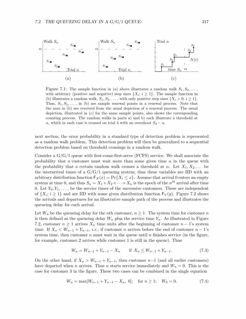
Figure 7.1 illustrates the difference between general random walks and positive random walks, i.e., renewal processes. Note that the renewal process in part b) is illustrated with the axes reversed from the conventional renewal process representation. We usually view each renewal epoch as a time (epoch) and view N(α) as the number of renewals up to time α, whereas with random walks, we usually view the number of trials as a discrete-time variable and view the sum of rv’s as some kind of amplitude or cost. There is no mathematical difference between these viewpoints, and each viewpoint is often helpful.

7.2 The queueing delay in a G/G/1 queue:

Before analyzing random walks in general, we introduce two important problem areas that are often best viewed in terms of random walks. In this section, the queueing delay in a G/G/1 queue is represented as a threshold crossing problem in a random walk. In the

317 7.2. THE QUEUEING DELAY IN A G/G/1 QUEUE:

α

S1

S2

S3

S4

S5

S1

S2 S3

S4

S5

S1

S2

S3

S4

S5

Walk Sn

α

Walk Sn

time Sn α

N(t)s s

s

s s

s

s s

s s

r r r r r

Trial n Trial n

Trial n

(a) (b) (c)

Figure 7.1: The sample function in (a) above illustrates a random walk S1, S2, . . . , with arbitrary (positive and negative) step sizes {Xi; i ≥ 1}. The sample function in (b) illustrates a random walk, S1, S2, . . . , with only positive step sizes {Xi > 0; i ≥ 1}. Thus, S1, S2, . . . , in (b) are sample renewal points in a renewal process. Note that the axes in (b) are reversed from the usual depiction of a renewal process. The usual depiction, illustrated in (c) for the same sample points, also shows the corresponding counting process. The random walks in parts a) and b) each illustrate a threshold at α, which in each case is crossed on trial 4 with an overshoot S4 − α.

next section, the error probability in a standard type of detection problem is represented as a random walk problem. This detection problem will then be generalized to a sequential detection problem based on threshold crossings in a random walk.

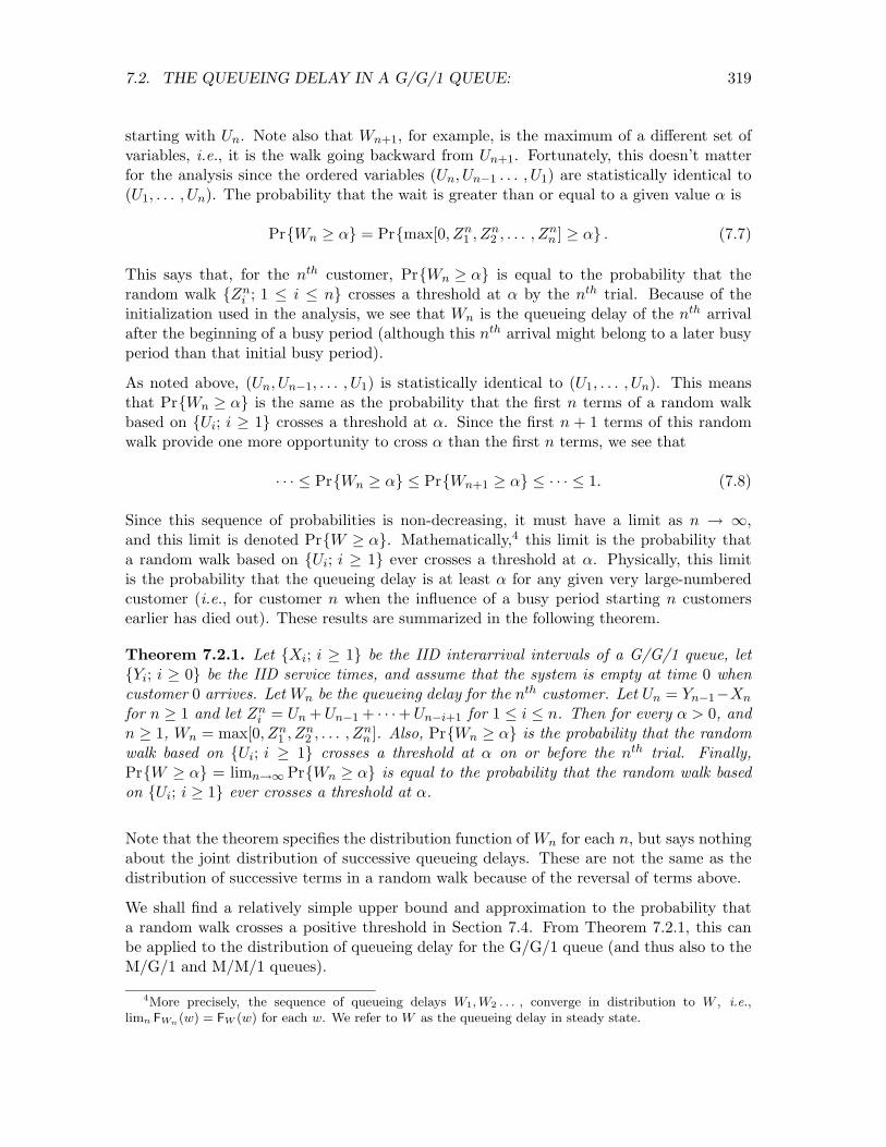
Consider a G/G/1 queue with first-come-first-serve (FCFS) service. We shall associate the probability that a customer must wait more than some given time α in the queue with the probability that a certain random walk crosses a threshold at α. Let X1,X2, . . . be the interarrival times of a G/G/1 queueing system; thus these variables are IID with an arbitrary distribution function FX (x) = Pr{Xi ≤ x}. Assume that arrival 0 enters an empty system at time 0, and thus Sn = X1 +X2 + +Xn is the epoch of the nth arrival after time · · ·0. Let Y0, Y1, . . . , be the service times of the successive customers. These are independent of {Xi; i ≥ 1} and are IID with some given distribution function FY (y). Figure 7.2 shows the arrivals and departures for an illustrative sample path of the process and illustrates the queueing delay for each arrival.

Let Wn be the queueing delay for the nth customer, n ≥ 1. The system time for customer n is then defined as the queueing delay Wn plus the service time Yn. As illustrated in Figure 7.2, customer n ≥ 1 arrives Xn time units after the beginning of customer n − 1’s system time. If Xn < Wn−1 + Yn−1, i.e., if customer n arrives before the end of customer n − 1’s system time, then customer n must wait in the queue until n finishes service (in the figure, for example, customer 2 arrives while customer 1 is still in the queue). Thus

Wn = Wn−1 + Yn−1 − Xn if Xn ≤ Wn−1 + Yn−1. (7.3)

On the other hand, if Xn > Wn−1 + Yn−1, then customer n−1 (and all earlier customers) have departed when n arrives. Thus n starts service immediately and Wn = 0. This is the case for customer 3 in the figure. These two cases can be combined in the single equation

Wn = max[Wn−1 + Yn−1 − Xn, 0]; for n ≥ 1; W0 = 0. (7.4)


s3

s2✛ x3 ✲✛ y3 ✲

s1Arrivals ✛ x2 ✲✛ w2 ✲✛ y2 ✲

0✛ x1 ✲✛ w1 ✲✛ y1 ✲ Departures

✛ y0 ✲

✛ ✲ x2 + w2 = w1 + y1

Figure 7.2: Sample path of arrivals and departures from a G/G/1 queue. Customer 0 arrives at time 0 and enters service immediately. Customer 1 arrives at time s1 = x1. For the case shown above, customer 0 has not yet departed, i.e., x1 < y0, so customer 1’s time in queue is w1 = y0 − x1. As illustrated, customer 1’s system time (queueing time plus service time) is w1 + y1.

Customer 2 arrives at s2 = x1 + x2. For the case shown above, this is before customer 1 departs at y0 + y1. Thus, customer 2’s wait in queue is w2 = y0 + y1 − x1 − x2. As illustrated above, x2 +w2 is also equal to customer 1’s system time, so w2 = w1 +y1 −x2. Customer 3 arrives when the system is empty, so it enters service immediately with no wait in queue, i.e., w3 = 0.

Since Yn−1 and Xn are coupled together in this equation for each n, it is convenient to define Un = Yn−1 − Xn. Note that {Un; n ≥ 1} is a sequence of IID random variables. From (7.4), Wn = max[Wn−1 + Un, 0], and iterating on this equation,

Wn = max[max[Wn−2+Un−1, 0]+Un, 0] = max[(Wn−2 + Un−1 + Un), Un, 0] = max[(Wn−3+Un−2+Un−1+Un), (Un−1+Un), Un, 0] = · · · · · · = max[(U1+U2+ . . . +Un), (U2+U3+ . . . +Un), . . . , (Un−1+Un), Un, 0]. (7.5)

It is not necessary for the theorem below, but we can understand this maximization better by realizing that if the maximization is achieved at Ui + Ui+1 + + Un, then a busy period · · · must start with the arrival of customer i − 1 and continue at least through the service of customer n. To see this intuitively, note that the analysis above starts with the arrival of customer 0 to an empty system at time 0, but the choice of 0 time and customer number 0 has nothing to do with the analysis, and thus the analysis is valid for any arrival to an empty system. Choosing the largest customer number before n that starts a busy period must then give the correct queueing delay, and thus maximizes (7.5). Exercise 7.2 provides further insight into this maximization.

Define Zn = Un, define Zn = Un + Un−1, and in general, for i ≤ n, define Zn = Un +Un−1 +1 2 i + Un−i+1. Thus Zn

n = Un + + U1. With these definitions, (7.5) becomes · · · · · ·

Wn = max[0, Z1 n, Z2

n, . . . , Znn]. (7.6)

Note that the terms in {Zn; 1 ≤ i ≤ n} are the first n terms of a random walk, but it i is not the random walk based on U1, U2, . . . , but rather the random walk going backward,

319 7.2. THE QUEUEING DELAY IN A G/G/1 QUEUE:

starting with Un. Note also that Wn+1, for example, is the maximum of a different set of variables, i.e., it is the walk going backward from Un+1. Fortunately, this doesn’t matter for the analysis since the ordered variables (Un, Un−1 . . . , U1) are statistically identical to (U1, . . . , Un). The probability that the wait is greater than or equal to a given value α is

Pr{Wn ≥ α} = Pr{max[0, Z1 n, Z2

n, . . . , Znn] ≥ α} . (7.7)

This says that, for the nth customer, Pr{Wn ≥ α} is equal to the probability that the random walk {Zn; 1 ≤ i ≤ n} crosses a threshold at α by the nth trial. Because of the i initialization used in the analysis, we see that Wn is the queueing delay of the nth arrival after the beginning of a busy period (although this nth arrival might belong to a later busy period than that initial busy period).

As noted above, (Un, Un−1, . . . , U1) is statistically identical to (U1, . . . , Un). This means that Pr{Wn ≥ α} is the same as the probability that the first n terms of a random walk based on {Ui; i ≥ 1} crosses a threshold at α. Since the first n + 1 terms of this random walk provide one more opportunity to cross α than the first n terms, we see that

· · · ≤ Pr{Wn ≥ α} ≤ Pr{Wn+1 ≥ α} ≤ · · · ≤ 1. (7.8)

Since this sequence of probabilities is non-decreasing, it must have a limit as n → 1, and this limit is denoted Pr{W ≥ α}. Mathematically,4 this limit is the probability that a random walk based on {Ui; i ≥ 1} ever crosses a threshold at α. Physically, this limit is the probability that the queueing delay is at least α for any given very large-numbered customer (i.e., for customer n when the influence of a busy period starting n customers earlier has died out). These results are summarized in the following theorem.

Theorem 7.2.1. Let {Xi; i ≥ 1} be the IID interarrival intervals of a G/G/1 queue, let {Yi; i ≥ 0} be the IID service times, and assume that the system is empty at time 0 when customer 0 arrives. Let Wn be the queueing delay for the nth customer. Let Un = Yn−1 −Xn

for n ≥ 1 and let Zin = Un + Un−1 + + Un−i+1 for 1 ≤ i ≤ n. Then for every α > 0, and · · ·

n ≥ 1, Wn = max[0, Z1 n, Z2

n, . . . , Zn]. Also, Pr{Wn ≥ α} is the probability that the random n walk based on {Ui; i ≥ 1} crosses a threshold at α on or before the nth trial. Finally, Pr{W ≥ α} = limn→1 Pr{Wn ≥ α} is equal to the probability that the random walk based on {Ui; i ≥ 1} ever crosses a threshold at α.

Note that the theorem specifies the distribution function of Wn for each n, but says nothing about the joint distribution of successive queueing delays. These are not the same as the distribution of successive terms in a random walk because of the reversal of terms above.

We shall find a relatively simple upper bound and approximation to the probability that a random walk crosses a positive threshold in Section 7.4. From Theorem 7.2.1, this can be applied to the distribution of queueing delay for the G/G/1 queue (and thus also to the M/G/1 and M/M/1 queues).

4More precisely, the sequence of queueing delays W1, W2 . . . , converge in distribution to W , i.e., limn FWn (w) = FW (w) for each w. We refer to W as the queueing delay in steady state.


7.3 Detection, decisions, and hypothesis testing

Consider a situation in which we make n noisy observations of the outcome of a single discrete random variable H and then guess, on the basis of the observations alone, which sample value of H occurred. In communication technology, this is called a detection problem. It models, for example, the situation in which a symbol is transmitted over a communication channel and n noisy observations are received. It similarly models the problem of detecting whether or not a target is present in a radar observation. In control theory, such situations are usually referred to as decision problems, whereas in statistics, they are referred to both as hypothesis testing and statistical inference problems.

The above communication, control, and statistical problems are basically the same, so we discuss all of them using the terminology of hypothesis testing. Thus the sample values of the rv H are called hypotheses. We assume throughout this section that H has only two possible values. Situations where H has more than 2 values can usually be viewed in terms of multiple binary decisions.

It makes no difference in the analysis of binary hypothesis testing what the two hypotheses happen to be called, so we simply denote them as hypothesis 0 and hypothesis 1. Thus H is a binary rv and we abbreviate its PMF as pH (0) = p0 and pH (1) = p1. Thus p0 and p1 = 1 − p0 are the a priori probabilities5 for the two sample values (hypotheses) of the random variable H.

Let Y = (Y1, Y2, . . . , Yn) be the n observations. Suppose, for initial simplicity, that these variables, conditional on H = 0 or H = 1, have joint conditional densities, fY |H (y | 0) and fY |H (y | 1), that are strictly positive over their common region of definition. The case of primary importance in this section (and the case where random walks are useful) is that in which, conditional on a given sample value of H, the rv’s Y1, . . . , Yn are IID. Still assuming for simplicity that the observations have densities, say fY |H (y | `) for ` = 0 or ` = 1, the joint density, conditional on H = `, is given by

n

fY |H (y | `) = Y

fY |H (yi | `). (7.9) i=1

Note that all components of Y are conditioned on the same H, i.e., for a single sample value of H, there are n corresponding sample values of Y .

5Statisticians have argued since the earliest days of statistics about the ‘validity’ of choosing a priori probabilities for the hypotheses to be tested. Bayesian statisticians are comfortable with this practice and non-Bayesians are not. Both are comfortable with choosing a probability model for the observations conditional on each hypothesis. We take a Bayesian approach here, partly to take advantage of the power of a complete probability model, and partly because non-Bayesian results, i.e., results that do not depend on the a priori probabilies, are often easier to derive and interpret within a collection of probability models using different choices for the a priori probabilities. As will be seen, the Bayesian approach also makes it natural to incorporate the results of earlier observations into updated a priori probabilities for analyzing later observations. In defense of non-Bayesians, note that the results of statistical tests are often used in areas of significant public policy disagreement, and it is important to give the appearance of a lack of bias. Statistical results can be biased in many more subtle ways than the use of a priori probabilities, but the use of an a priori distribution is particularly easy to attack.

321 7.3. DETECTION, DECISIONS, AND HYPOTHESIS TESTING

Assume that it is necessary6 to select a sample value for H on the basis of the sample value y of the n observations. It is usually possible for the selection (decision) to be incorrect, so we distinguish the sample value h of the actual experimental outcome from the sample value h of our selection. That is, the outcome of the experiment specifies h and y , but only y is observed. The selection h, based only on y , might be unequal to h. We say that an error has occurred if h =6 h

We now analyze both how to make decisions and how to evaluate the resulting probability of error. Given a particular sample of n observations y = y1, y2, . . . , yn, we can evaluate Pr{H=0 | y} as

Pr{H=0 p0fY |H (y | 0)

(7.10)| y} = p0fY |H (y | 0) + p1fY |H (y | 1)

.

We can evaluate Pr{H=1 | y} in the same way The ratio of these quantities is given by

Pr{H=0 | y} =

p0fY |H (y | 0) (7.11)

Pr{H=1 | y} p1fY |H (y | 1).

For a given y , if we select h = 0, then an error is made if h = 1. The probability of this event is Pr{H = 1 | y}. Similarly, if we select h = 1, the probability of error is Pr{H = 0 | y}. Thus the probability of error is minimized, for a given y , by selecting h=0 if the ratio in (7.11) is greater than 1 and selecting h=1 otherwise. If the ratio is equal to 1, the error probability is the same whether h=0 or h=1 is selected, so we arbitrarily select h = 1 to make the rule deterministic.

The above rule for choosing H=0 or H=1 is called the Maximum a posteriori probability detection rule, abbreviated as the MAP rule. Since it minimizes the error probability for each y , it also minimizes the overall error probability as an expectation over Y and H.

The structure of the MAP test becomes clearer if we define the likelihood ratio Λ(y) for the binary decision as

fY |H (y 0)Λ(y) =

fY |H (y

|| 1)

.

The likelihood ratio is a function only of the observation y and does not depend on the a priori probabilities. There is a corresponding rv Λ(Y ) that is a function7 of Y , but we will tend to deal with the sample values. The MAP test can now be compactly stated as

> p1/p0 ; select h=0

Λ(y) (7.12) ≤ p1/p0 ; select h=1.

6In a sense, it is in making decisions where the rubber meets the road. For real-world situations, a probabilistic analysis is often connected with studying the problem, but eventually one technology or another must be chosen for a system, one person or another must be hired for a job, one law or another must be passed, etc.

7Note that in a non-Bayesian formulation, Y is a different random vector, in a different probability space, for H = 0 than for H = 1. However, the corresponding conditional probabilities for each exist in each probability space, and thus Λ(Y ) exists (as a different rv) in each space.


For the primary case of interest, where the n observations are IID conditional on H, the likelihood ratio is given by

Λ(y) = Yn fY |H (yi | 0)

i=1 fY |H (yi | 1).

The MAP test then takes on a more attractive form if we take the logarithm of each side in (7.12). The logarithm of Λ(y) is then a sum of n terms,

Pni=1 zi, where zi is given by

fY |H (yi 0) zi = ln

fY |H (yi

|| 1)

.

The sample value zi is called the log-likelihood ratio of yi for each i, and ln Λ(y) is called the log-likelihood ratio of y . The test in (7.12) is then expressed as

nX

i=1

zi

> ln(p1/p0) ; select h=0

(7.13)≤ ln(p1/p0) ; select h=1.

As one might imagine, log-likelihood ratios are far more convenient to work with than likelihood ratios when dealing with conditionally IID rv’s.

Example 7.3.1. Consider a Poisson process for which the arrival rate ∏ might be ∏0 or might be ∏1. Assume, for i ∈ {0, 1}, that pi is the a priori probability that the rate is ∏i. Suppose we observe the first n arrivals, Y1, . . . Yn and make a MAP decision about the arrival rate from the sample values y1, . . . , yn.

The conditional probability densities for the observations Y1, . . . , Yn are given by

fY |H (y | i) = Yn

i=1 ∏ie

−∏iyi .

The test in (7.13) then becomes

n ln(∏0/∏1) + Xn

i=1

(∏1 − ∏0)yi


≤ ln(p1/p0) ; select h=1.

Note that the test depends on y only through the time of the nth arrival. This should not be surprising, since we know that, under each hypothesis, the first n − 1 arrivals are uniformly distributed conditional on the nth arrival time.

The MAP test in (7.12), and the special case in (7.13), are examples of threshold tests. That is, in (7.12), a decision is made by calculating the likelihood ratio and comparing it to a threshold η = p1/p0. In (7.13), the log-likelihood ratio ln(Λ(y)) is compared with ln η = ln(p1/p0).

There are a number of other formulations of hypothesis testing that also lead to threshold tests, although in these alternative formulations, the threshold η > 0 need not be equal to


p1/p0, and indeed a priori probabilities need not even be defined. In particular, then, the threshold test at η is defined by

> η ; select h=0

Λ(y) (7.14); select h=1. ≤ η

For example, maximum likelihood (ML) detection selects hypothesis h = 0 if fY |H (y | 0) >

fY |H (y | 1), and selects h = 1 otherwise. Thus the ML test is a threshold test with η = 1. Note that ML detection is equivalent to MAP detection with equal a priori probabilities, but it can be used in many other cases, including those with undefined a priori probabilities.

In many detection situations there are unequal costs, say C0 and C1, associated with the two kinds of errors. For example one kind of error in a medical prognosis could lead to serious illness and the other to an unneeded operation. A minimum cost decision could then minimize the expected cost over the two types of errors. As shown in Exercise 7.5, this is also a threshold test with the threshold η = (C1p1)/(C0p0). This example also illustrates that, although assigning costs to errors provides a rational approach to decision making, there might be no widely agreeable way to assign costs.

Finally, consider the situation in which one kind of error, say Pr{e | H=1} is upper bounded by some tolerable limit α and Pr{e | H=0} is minimized subject to this constraint. The solution to this is called the Neyman-Pearson rule. The Neyman-Pearson rule is of particular interest since it does not require any assumptions about a priori probabilities. The next subsection shows that the Neyman-Pearson rule is essentially a threshold test, and explains why one rarely looks at tests other than threshold tests.

7.3.1 The error curve and the Neyman-Pearson rule

Any test, i.e., any deterministic rule for selecting a binary hypothesis from an observation y , can be viewed as a function8 mapping each possible observation y to 0 or 1. If we define A as the set of n-vectors y that are mapped to hypothesis 1 for a given test, then the test can be identified by its corresponding set A.

Given the test A, the error probabilities, given H = 0 and H = 1 respectively, are given by

Pr{Y ∈ A | H = 0} ; Pr{Y ∈ Ac | H = 1} .

Note that these conditional error probabilities depend only on the test A and not on the a priori probabilities. We will abbreviate these error probabilities as

q0(A) = Pr{Y ∈ A | H = 0} ; q1(A) = Pr{Y ∈ Ac | H = 1} .

For given a priori probabilities, p0 and p1, the overall error probability is

Pr{e(A)} = p0q0(A) + p1q1(A). 8By assumption, the decision must be made on the basis of the observation y , so a deterministic rule is

based solely on y , i.e., is a function of y . We will see later that randomized rather than deterministic rules are required for some purposes, but such rules are called randomized rules rather than tests.


If A is a threshold test, with threshold η, the set A is given by

A =

Ω

y : fY |H (y | 0) æ

. fY |H (y | 1)

≤ η

Since threshold tests play a very special role here, we abuse the notation by using η in place of A to refer to a threshold test at η. We can now characterize the relationship between threshold tests and other tests. The following lemma is illustrated in Figure 7.3.

Lemma 7.3.1. Consider a two dimensional plot in which the error probabilities for each test A are plotted as (q1(A), q0(A)). Then for any theshold test η, 0 < η < 1, and any A, the point (q1(A), q0(A)) is on the closed half plane above and to the right of a straight line of slope −η passing through the point (q1(η), q0(η)).

1

q0(A) + ηq1(A)

q0(η) + ηq1(η)

q0(η)

❜❜❜❜❜❜❜❜❜❜❜❜ 1q1(η)

slope −η s

s(q1(A), q0(A))❜❜❜❜❜

qi(A) = Pr{e | H=i} for test A

Figure 7.3: Illustration of Lemma 7.3.1

Proof: For any given η, consider the a priori probabilities9 (p0, p1) for which η = p1/p0. The overall error probability for test A using these a priori probabilities is then

Pr{e(A)} = p0q0(A) + p1q1(A) = p0£q0(A) + ηq1(A)

§.

Similarly, the overall error probability for the threshold test η using the same a priori probabilities is

Pr{e(η)} = p0q0(η) + p1q1(η) = p0 £q0(η) + ηq1(η)

§.

This latter error probability is the MAP error probability for the given p0, p1, and is thus the minimum overall error probability (for the given p0, p1) over all tests. Thus

q0(η) + ηq1(η) ≤ q0(A) + ηq1(A).

As shown in the figure, these are the points at which the lines of slope −η from (q1(A), q0(A)) and (q1(η), q0(η)) respectively cross the ordinate axis. Thus all points on the first line

9Note that the lemma does not assume any a priori probabilities. The MAP test for each a priori choice (p0, p1) determines q0(η) and q1(η) for η = p1/p0. Its interpretation as a MAP test depends on a model with a priori probabilities, but its calculation depends only on p0, p1 viewed as parameters.


(including (q1(A), q0(A))) lie in the closed half plane above and to the right of all points on the second, completing the proof.

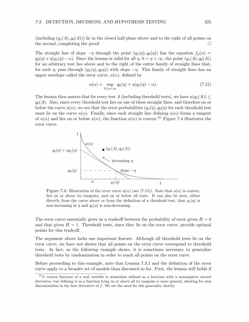
The straight line of slope −η through the point (q1(η), q0(η)) has the equation fη(α) = q0(η)+ η(q1(η) − α). Since the lemma is valid for all η, 0 < η < 1, the point (q1(A), q0(A)) for an arbitrary test lies above and to the right of the entire family of straight lines that, for each η, pass through (q1(η), q0η)) with slope −η. This family of straight lines has an upper envelope called the error curve, u(α), defined by

u(α) = sup q0(η) + η(q1(η) − α). (7.15) 0≤η<1

The lemma then asserts that for every test A (including threshold tests), we have u(q1(A)) ≤ q0(A). Also, since every threshold test lies on one of these straight lines, and therefore on or below the curve u(α), we see that the error probabilities (q1(η), q0(η) for each threshold test must lie on the curve u(α). Finally, since each straight line defining u(α) forms a tangent of u(α) and lies on or below u(α), the function u(α) is convex.10 Figure 7.4 illustrates the error curve.

❜❜❜❜❜❜❜❜❜❜❜❜

q0(η) + ηq1(η)

q0(η)

1

slope −η

◗◗❦ increasing η

t(q1(A), q0(A)) u(α)

α q1(η) 1

Figure 7.4: Illustration of the error curve u(α) (see (7.15)). Note that u(α) is convex, lies on or above its tangents, and on or below all tests. It can also be seen, either directly from the curve above or from the definition of a threshold test, that q1(η) is non-increasing in η and q0(η) is non-decreasing.

The error curve essentially gives us a tradeoff between the probability of error given H = 0 and that given H = 1. Threshold tests, since they lie on the error curve, provide optimal points for this tradeoff.

The argument above lacks one important feature. Although all threshold tests lie on the error curve, we have not shown that all points on the error curve correspond to threshold tests. In fact, as the following example shows, it is sometimes necessary to generalize threshold tests by randomization in order to reach all points on the error curve.

Before proceeding to this example, note that Lemma 7.3.1 and the definition of the error curve apply to a broader set of models than discussed so far. First, the lemma still holds if

10A convex function of a real variable is sometimes defined as a function with a nonnegative second derivative, but defining it as a function lying on or above all its tangents is more general, allowing for step discontinuities in the first derivative of f . We see the need for this generality shortly.


fY |H (y | `) is zero over an arbitrary set of y for one or both hypotheses `. The likelihood ratio Λ(y) is infinite where fY |H (y | 0) > 0 and fY |H (y | 1) = 0, but this does not affect the proof of the lemma. Exercise 7.6 helps explain how this situation can affect the error curve.

In addition, it can be seen that the lemma also holds if Y is an n-tuple of discrete rv’s. The following example further explains the discrete case and also shows why not all points on the error curve correspond to threshold tests. What we assume throughout is that Λ(Y ) is a rv conditional on H = 1 and is a possibly-defective11 rv conditional on H = 0.

Example 7.3.2. About the simplest example of a detection problem is that with a one-dimensional binary observation Y . Assume then that

2 1 pY |H (0 | 0) = pY |H (1 | 1) =

3; pY |H (0 | 1) = pY |H (1 | 0) =

3.

Thus the observation Y equals H with probability 2/3. The ‘natural’ decision rule would be to select h to agree with the observation y, thus making an error with probability 1/3, both conditional on H = 1 and H = 0. It is easy to verify from (7.12) (using PMF’s in place of densities) that this ‘natural’ rule is the MAP rule if the a priori probabilities are in the range 1/3 ≤ p1 < 2/3.

For p1 < 1/3, the MAP rule can be seen to be h = 0, no matter what the observation is. Intuitively, hypothesis 1 is too unlikely a priori to be overcome by the evidence when Y = 1. Similarly, if p1 ≥ 2/3, then the MAP rule selects h = 1, independent of the observation.

The corresponding threshold test (see (7.14)) selects h = y for 1/2 ≤ η < 2. It selects h = 0 for η < 1/2 and h = 1 for η ≥ 2. This means that, although there is a threshold test for each η, there are only 3 resulting error probability pairs, i.e., (q1(η), q0(η) can be (0, 1) or (1/3, 1/3), or (1, 0). The first pair holds for η ≥ 2, the second for 1/2 ≤ η < 2, and the third for η < 1/2. This is illustrated in Figure 7.5.

We have just seen that there is a threshold test for each η, 0 < η < 1, but those threshold tests map to only 3 distinct points (q1(η), q0(η)). As can be seen, the error curve joins these 3 points by straight lines.

Let us look more carefully at the tangent of slope -1/2 through the point (1/3, 1/3. This corresponds to the MAP test at p1 = 1/3. As seen in (7.12), this MAP test selects h = 1 for y = 1 and h = 0 for y = 0. The selection of h = 1 when y = 1 is a don’t-care choice in which selecting h = 0 would yield the same overall error probability, but would change (q1(η), q0(η) from (1/3, 1/3) to (1, 0).

It is not hard to verify (since there are only 4 tests, i.e., deterministic rules, for mapping a binary variable to another binary variable) that no test can achieve the tradeoff between q1(A) and q0(A) indicated by the interior points on the straight line between (1/3, 1/3) and (1, 0). However, if we use a randomized rule, mapping 1 to 1 with probability θ and into 0 with probability 1 − θ (along with always mappng 0 to 0), then all points on the straight

11If pY |H (y | 1) = 0 and pY |H (y | 0) > 0 for some y , then Λ(y) is infinite, and thus defective, conditional on H = 0. Since the given y has zero probability conditional on H = 0, we see that Λ(Y ) is not defective conditional on H = 1.


q0(η)

1 (0, 1)

1

(1, 0)

(1/3. 1/3)

q1(η)

slope −1/2

slope −2

Figure 7.5: Illustration of the error curve u(α) for Example 7.3.2. For all η in the range 1/2 ≤ η < 2, the threshold test selects h = y. The corresponding error probabilities are then q1(η) = q0(η) = 1/3. For η < 1/2, the threshold test selects h = 0 for all y, and for η > 2, it selects h = 1 for all y. The error curve (see (7.15)) for points to the right of (1/3, 1/3) is maximized by the straight line of slope -1/2 through (1/3, 1/3). Similarly, the error curve for points to the left of (1/3, 1/3) is maximized by the straight line of slope -2 through (1/3, 1/3). One can visualize the tangent lines as an inverted see-saw, first see-sawing around (0,1), then around (1/3, 1/3), and finally around (1, 0).

line from (1/3, 1/3) to (1, 0) are achieved as θ goes from 0 to 1. In other words, a don’t-care choice for MAP becomes an important choice in the tradeoff between q1(A) and q0(A).

In the same way, all points on the straight line from (0, 1) to (1/3, 1/3) can be achieved by a randomized rule that maps 0 to 0 with given probability θ (along with always mapping 1 to 1).

In the general case, the error curve can contain straight line segments whenever the distribution function of the likelihood ratio, conditional on H = 1, is discontinuous. This is always the case for discrete observations, and, as illustrated in Exercise 7.6, might also occur with continuous observations. To understand this, suppose that Pr{Λ(Y ) = η | H=1} = β > 0 for some η, 0 < η < 1. Then the MAP test at η has a don’t-care region of probability β given H = 1. This means that if the MAP test is changed to resolve the don’t-care case in favor of H = 0, then the error probability q1 is increased by β and the error probability q0 is decreased by ηβ. Lemma 7.3.1 is easily seen to be valid whichever way the don’t-care cases are resolved, and thus both (q1, q0) and (q1+β, q0−ηβ) lie on the error curve. Since all tests lie above and to the right of the straight line of slope −η through these points, the error curve has a straight line segment between these points. As mentioned before, any pair of error probabilities on this straight line segment can be realized by using a randomized threshold test at η.

The Neyman-Pearson rule is the rule (randomized where needed) that realizes any desired error probability pair (q1, q0) on the error curve, i.e., where q0 = u(q1). To be specific, assume the constraint that q1 = α for any given α, 0 < α ≤ 1. Since Pr{Λ(Y ) > η | H = 1}is a complementary distribution function, it is non-increasing in η, perhaps with step discontinuities. At η = 0, it has the value 1 − Pr{Λ(Y ) = 0}. As η increases, it decreases to 0, either for some finite η or as η →1. Thus if 0 < α ≤ 1 − Pr{Λ(Y ) = 0}, we see that α is either equal to Pr{Λ(y) > η | H = 1} for some η or α is on a step discontinuity at some


η. Defining η(α) as an η where one of these alternatives occur,12 there is a solution to the following:

Pr{Λ(y)>η(α) | H=1} ≤ α ≤ Pr{Λ(y)≥η(α) | H=1} . (7.16)

Note that (7.16) also holds, with η(α) = 0 if 1 − Pr{Λ(Y )=0} < α ≤ 1.

The Neyman-Pearson rule, given α, is to use a threshold test at η(α) if Pr{Λ(y)=η(α) | H=1} = 0. If Pr{Λ(y)=η(α) | H=1} > 0, then a randomized test is used at η(α). When Λ(y) = η(α), h is chosen to be 1 with probability θ where

θ = α − Pr{Λ(y) > η(α) | H = 1}

. (7.17)Pr{Λ(y) = η(α) | H = 1}

This is summarized in the following theorem:

Theorem 7.3.1. Assume that the likelihood ratio Λ(Y) is a rv under H = 1. For any α, 0 < α ≤ 1, the constraint that Pr{e | H = 1} ≤ α implies that Pr{e | H = 0} ≥ u(α) where u(α) is the error curve. Furthermore, Pr{e | H = 0} = u(α) if the Neyman-Pearson rule, specified in (7.16) and (7.17), is used.

Proof: We have shown that the Neyman-Pearson rule has the stipulated error probabilities. An arbitrary decision rule, randomized or not, can be specified by a finite set A1, . . . , Ak

of deterministic decision rules along with a rv V , independent of H and Y , with sample values 1, . . . , k. Letting the PMF of V be (θ1, . . . , θk), an arbitrary decision rule, given Y = y and V = i is to use decision rule Ai if V = i. The error probabilities for this rule are Pr{e | H=1} =

Pk θiq1(Ai) and Pr{e | H=0} = Pk θiq0(Ai). It is easy to see that i=1 i=1

Lemma 7.3.1 applies to these randomized rules in the same way as to deterministic rules.

All of the decision rules we have discussed are threshold rules, and in all such rules, the first part of the decision rule is to find the likelihood ratio Λ(y) from the observation y . This simplifies the hypothesis testing problem from processing an n-dimensional vector y to processing a single number Λ(y), and this is typically the major component of making a threshold decision. Any intermediate calculation from y that allows Λ(y) to be calculated is called a sufficient statistic. These usually play an important role in detection, especially for detection in noisy environments.

There are some hypothesis testing problems in which threshold rules are in a sense inappropriate. In particular, the cost of an error under one or the other hypothesis could be highly dependent on the observation y . A minimum cost threshold test for each y would still be appropriate, but a threshold test based on the likelihood ratio might be inappropriate since different observations with very different cost structures could have the same likelihood ratio. In other words, in such situations, the likelihood ratio is no longer sufficient to make a minimum cost decision.

12In the discrete case, there can be multiple solutions to (7.16) for some values of α, but this does not affect the decision rule. One can choose the smallest value of η to satisfy (7.16) if one wants to eliminate this ambiguity.

7.4. THRESHOLD CROSSING PROBABILITIES IN RANDOM WALKS 329

So far we have assumed that a decision is made after a predetermined number n of observations. In many situations, observations are costly and introduce an unwanted delay in decisions. One would prefer, after a given number of observations, to make a decision if the resulting probability of error is small enough, and to continue with more observations otherwise. Common sense dictates such a strategy, and the branch of probability theory analyzing such strategies is called sequential analysis. In a sense, this is a generalization of Neyman-Pearson tests, which employed a tradeoff between the two types of errors. Here we will have a three-way tradeoff between the two types of errors and the time required to make a decision.

We now return to the hypothesis testing problem of major interest where the observations, conditional on the hypothesis, are IID. In this case the log-likelihood ratio after n observations is the sum Sn = Z1 + Zn of the n IID individual log likelihood ratios. Thus, aside · · · from the question of making a decision after some number of observations, the sequence of log-likelihood ratios S1, S2, . . . is a random walk.

Essentially, we will see that an appropriate way to choose how many observations to make, based on the result of the earlier observations, is as follows: The probability of error under either hypothesis is based on Sn = Z1 + + Zn. Thus we will see that an appropriate · · · rule is to choose H=0 if the sample value sn of Sn is more than some positive threshold α, to choose H1 if sn ≤ β for some negative threshold β, and to continue testing if the sample value has not exceeded either threshold. In other words, the decision time for these sequential decision problems is the time at which the corresponding random walk crosses a threshold. An error is made when the wrong threshold is crossed.

We have now seen that both the queueing delay in a G/G/1 queue and the above sequential hypothesis testing problem can be viewed as threshold crossing problems for random walks. The following section begins a systemic study of such problems.

7.4 Threshold crossing probabilities in random walks

Let {Xi; i ≥ 1} be a sequence of IID random variables (rv’s ), each with the distribution function FX (x), and let {Sn; n ≥ 1} be a random walk with Sn = X1 + + Xn. Let· · · gX (r) = E

£erX

§ be the MGF of X and let r and r+ be the upper and lower ends of the −

interval over which g(r) is finite. We assume throughout that r− < 0 < r+. Each of r− and r+ might be contained in the interval where gX (r) is finite, and each of r and r+ might −be infinite.

The major objective of this section is to develop results about the probability that the sequence {Sn; n ≥ 1} ever crosses a given threshold α > 0, i.e., Pr{

S1n=1{Sn ≥ α}}. We as

sume throughout this section that X < 0 and that X takes on both positive and negative values with positive probability. Under these conditions, we will see that Pr{

S1n=1{Sn ≥ α}}

is essentially bounded by an exponentially decreasing function of α. In this section and the next, this exponent is evaluated and shown to be exponentially tight with increasing α. The next section also finds an exponentially tight bound on the probability that a threshold at α is crossed before another threshold at β < 0 is crossed.


7.4.1 The Chernoff bound

The Chernoff bound was derived and discussed in Section 1.4.3. It was shown in (1.62) that for any r ∈ (0, r+) and any a > X, that

Pr{Sn ≥ na} ≤ exp (n[∞X (r) − ra]) . (7.18)

where ∞X (r) = ln gX (r) is the semi-invariant MGF of X. The tightest bound of this form is given by

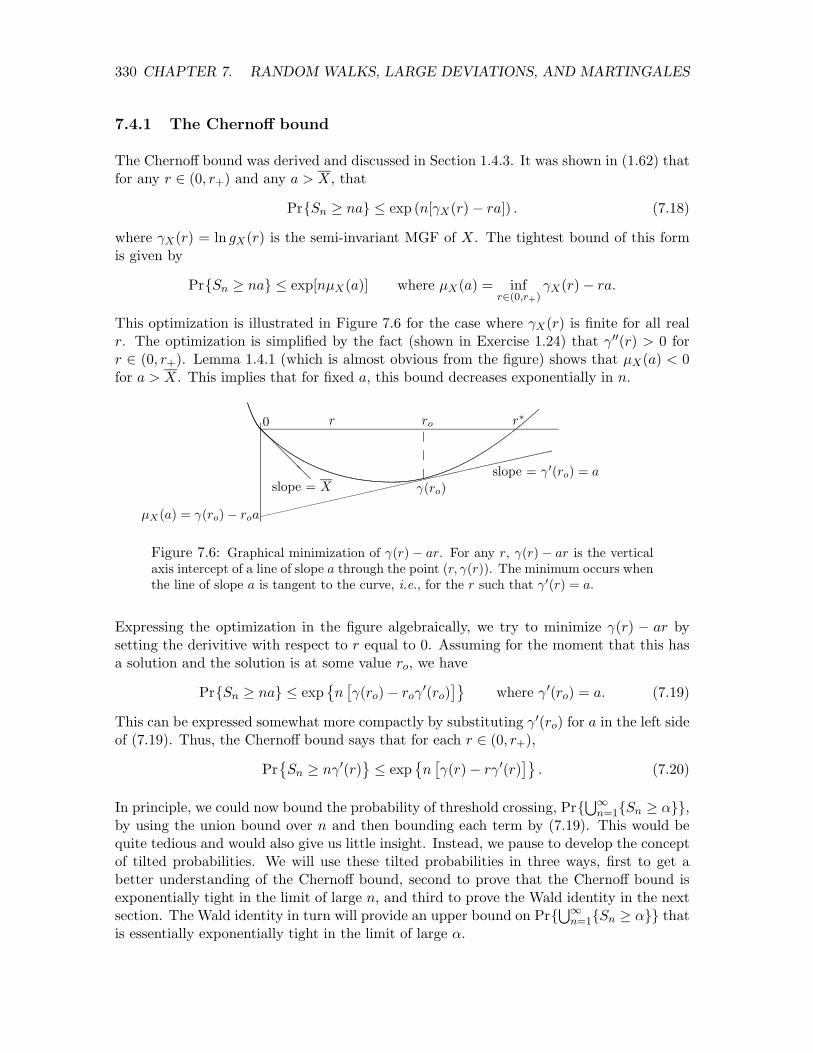
Pr{Sn ≥ na} ≤ exp[nµX (a)] where µX (a) = inf ∞X (r) − ra. r∈(0,r+)

This optimization is illustrated in Figure 7.6 for the case where ∞X (r) is finite for all real r. The optimization is simplified by the fact (shown in Exercise 1.24) that ∞00(r) > 0 for r ∈ (0, r+). Lemma 1.4.1 (which is almost obvious from the figure) shows that µX (a) < 0 for a > X. This implies that for fixed a, this bound decreases exponentially in n.

0 r ro r∗

❅ ❅

❅ ❅ slope = ∞0(ro) = a

slope = X ∞(ro)

µX (a) = ∞(ro) − roa

Figure 7.6: Graphical minimization of ∞(r) − ar. For any r, ∞(r) − ar is the vertical axis intercept of a line of slope a through the point (r, ∞(r)). The minimum occurs when the line of slope a is tangent to the curve, i.e., for the r such that ∞0(r) = a.

Expressing the optimization in the figure algebraically, we try to minimize ∞(r) − ar by setting the derivitive with respect to r equal to 0. Assuming for the moment that this has a solution and the solution is at some value ro, we have

Pr{Sn ≥ na} ≤ exp ©n

£∞(ro) − ro∞

0(ro)§™

where ∞0(ro) = a. (7.19)

This can be expressed somewhat more compactly by substituting ∞0(ro) for a in the left side of (7.19). Thus, the Chernoff bound says that for each r ∈ (0, r+),

Pr©Sn ≥ n∞0(r)

™ ≤ exp

©n

£∞(r) − r∞0(r)

§™ . (7.20)

In principle, we could now bound the probability of threshold crossing, Pr{S1

n=1{Sn ≥ α}}, by using the union bound over n and then bounding each term by (7.19). This would be quite tedious and would also give us little insight. Instead, we pause to develop the concept of tilted probabilities. We will use these tilted probabilities in three ways, first to get a better understanding of the Chernoff bound, second to prove that the Chernoff bound is exponentially tight in the limit of large n, and third to prove the Wald identity in the next section. The Wald identity in turn will provide an upper bound on Pr{

S1n=1{Sn ≥ α}} that

is essentially exponentially tight in the limit of large α.


7.4.2 Tilted probabilities

As above, let {Xn; n ≥ 1} be a sequence of IID rv’s and assume that gX (r) is finite for r ∈ (r−, r+). Initially assume that X is discrete with the PMF pX (x) for each sample value x of X. For any given r ∈ (r−, r+), define a new PMF (called a tilted PMF) on X by

qX,r(x) = pX (x) exp[rx − ∞(r)]. (7.21)

Note that qX,r(x) ≥ 0 for all sample values x and P

qX,r(x) = P

pX (x)erx/E [erx] = 1, x x so this is a valid probability assignment.

Imagine a random walk, summing IID rv’s Xi, using this new probability assignment rather than the old. We then have the same mapping from sample points of the underlying sample space to sample values of rv’s, but we are dealing with a new probability space, i.e., we have changed the probability model, and thus we have changed the probabilities in the random walk. We will further define this new probability measure so that the rv’s X1,X2, . . . in this new probability space are IID.13 For every event in the old walk, the same event exists in the new walk, but its probability has changed.

Using (7.21), along with the assumption that X1,X2, . . . are independent in the tilted probability assignment, the tilted PMF of an n tuple X = (X1,X2, . . . ,Xn) is given by

n

qX n,r(x1, . . . , xn) = pX n (x1, . . . , xn) exp( X

[rxi − ∞(r)]. (7.22) i=1

Next we must related the PMF of the sum, Pn

i=1 Xi, in the original probability measure to that in the tilted probability measure. From (7.22), note that for every n-tuple (x1, . . . , xn) for which

Pni=1 xi = sn (for any given sn) we have

qX n,r(x1, . . . , xn) = pX n (x1, . . . , xn) exp[rsn − n∞(r)].

nSumming over all x for which Pn

i=1 xi = sn, we then get a remarkable relation between the PMF for Sn in the original and the tilted probability measures:

qSn,r(sn) = pSn (sn) exp[rsn − n∞(r)]. (7.23)

This equation is the key to large deviation theory applied to sums of IID rv’s . The tilted measure of Sn, for positive r, increases the probability of large values of Sn and decreases that of small values. Since Sn is an IID sum under the tilted measure, however, we can use the laws of large numbers and the CLT around the tilted mean to get good estimates and bounds on the behavior of Sn far from the mean for the original measure.

13One might ask whether X1, X2, . . . are the same rv’s in this new probability measure as in the old. It is usually convenient to view them as being the same, since they correspond to the same mapping from sample points to sample values in both probability measures. However, since the probability space has changed, one can equally well view them as different rv’s. It doesn’t make any difference which viewpoint is adopted, since all we use the relationship in (7.21), and other similar relationships, to calculate probabilities in the original system.


We now denote the mean of X in the tilted measure as Er[X]. Using (7.21),

Er[X] = X

xqX,r(x) = X

xpX (x) exp[rx − ∞(r)] x x

1 d =

gX (r)

X

dr pX (x) exp[rx]

x

g0 (r)= X = ∞0(r). (7.24)

gX (r)

Higher moments of X under the tilted measure can be calculated in the same way, but, more elegantly, the MGF of X under the tilted measure can be seen to be Er[exp(tX)] = gX (t + r)/gX (r).

The following theorem uses (7.23) and (7.24) to show that the Chernoff bound is exponentially tight.

Theorem 7.4.1. Let {Xn; n ≥ 1} be a discrete IID sequence with a finite MGF for r ∈(r−, r+) where r− < 0 < r+. Let Sn =

Pn for each n ≥ 1. Then for any r ∈ (0, r+),i=1 xi

and any ≤ > 0 and δ > 0 there is an m such that for all n ≥ m,

Pr©Sn ≥ n(∞0(r) − ≤)

™ ≥ (1 − δ) exp[n(∞(r) − r∞0(r) − r≤)]. (7.25)

Proof: The weak law of large numbers, in the form of (1.76), applies to the tilted measure on each Sn. Writing out the limit on n there, we see that for any ≤, δ, there is an m such that for all n ≥ m,

1 − δ ≤ X

qSn,r(sn)(∞0(r)−≤)n ≤ sn ≤ (∞0(r)+≤)n

= X

pSn (sn) exp[rsn − n∞(r)] (7.26) (∞0(r)−≤)n ≤ sn ≤ (∞0(r)+≤)n

≤ X

pSn (sn) exp[n(r∞0(r) + r≤ − ∞(r))] (7.27) (∞0(r)−≤)n ≤ sn ≤ (∞0(r)+≤)n

≤ X

pSn (sn) exp[n(r∞0(r) + r≤ − ∞(r))] (7.28) (∞0(r)−≤)n ≤ sn

= exp[n(r∞0(r) + r≤ − ∞(r))] Pr©Sn ≥ n(∞0(r) − ≤)

™ . (7.29)

The equality (7.26) follows from (7.23) and the inequality (7.27) follows because sn ≤∞0(r) + ≤ in the sum. The next inequality is the result of adding additional positive terms into the sum, and (7.29) simply replaces the sum over a PMF with the probability of the given event. Since (7.29) is equivalent to (7.25), the proof is complete.

The structure of the above proof can be used in many situations. A tilted probability measure is used to focus on the tail of a distribution, and then some known result about the tilted distribution is used to derive the desired result about the given distribution.


7.4.3 Back to threshold crossings

The Chernoff bound is convenient (and exponentially tight) for understanding Pr{Sn ≥ na}as a function of n for fixed a. It does not give us as much direct insight into Pr{Sn ≥ α} as a function of n for fixed α, which tells us something about when a threshold at α is most likely to be crossed. Additional insight can be achieved by substituing α/∞0(r0) for n in (7.19), getting

Ω ∑ ∞(ro)

∏æ

Pr{Sn ≥ α} ≤ exp α∞0(ro)

− ro where ∞0(ro) = α/n. (7.30)

A nice graphic interpretation of this equation is given in Figure 7.7. Note that the exponent in α, namely ∞(r0)/∞0(r0) − r0 is the negative of the horizontal axis intercept of the line of slope ∞0(r0) = α/n in Figure 7.7.

❅ 0 r ro r∗ ro − ∞(ro)/∞0(r0)

❅ ❅

❅ slope = ∞0(ro) = α/n slope = X ∞(ro)

Figure 7.7: The exponent in α for Pr{Sn ≥ α}, minimized over r. The minimization is the same as that in Figure 7.6, but ∞(ro)/∞0(ro) − ro is the negative of the horizontal axis intercept of the line tangent to ∞(r) at r = r0.

For fixed α, then, we see that for very large n, the slope α/n is very small and this horizontal intercept is very large. As n is decreased, the slope increases, r0 increases, and the horizontal intercept decreases. When r0 increases to the point labeled r∗ in the figure, namely the r > 0 at which ∞(r) = 0, then the exponent decreases to r∗. When n decreases even further, r0 becomes larger than r∗ and the horizontal intercept starts to increase again.

Since r∗ is the minimum horizontal axis intercept of this class of straight lines, we see that the following bound holds for all n,

Pr{Sn ≥ α} ≤ exp(−r∗α) for arbitrary α > 0, n ≥ 1, (7.31)

where r∗ is the positive root of ∞(r) = 0.

The graphical argument above assumed that there is some r∗ > 0 such that ∞X (r∗) = 0. However, if r+ = 1, then (since X takes on positive values with positive probability by assumption) ∞(r) can be seen to approach 1 as r →1. Thus r∗ must exist because of the continuity of ∞(r) in (r−, r+). This is summarized in the following lemma.

Lemma 7.4.1. Let {Sn = X1 + + Xn; n ≥ 1} be a random walk where {Xi; i ≥ 1}· · · is an IID sequence where gX (r) exists for all r ≥ 0, where X < 0, and where X takes on both positive and negative values with positive probability. Then for all integer n > 0 and


all α > 0

Pr{Sn ≥ α} ≤ exp{α[∞(r0)n/α − r0]} ≤ exp(−r∗α). (7.32)

where ∞0(ro) = α/n.

Next we briefly consider the situation where r+ < 1. There are two cases to consider, first where ∞(r+) is infinite and second where it is finite. Examples of these cases are given in Exercise 1.22, parts b) and c) respectively. For the case ∞(r+) = 1, Exercise 1.23 shows that ∞(r) goes to 1 as r increases toward r+. Thus r∗ must exist in this case 1 by continuity.

The case ∞(r+) < 1 is best explained by Figure 7.8. As explained there, if ∞0(r) = α/n for some r0 < r+, then (7.19) and (7.30) hold as before. Alternatively, if α/n > ∞0(r) for all r < r+, then the Chernoff bound is optimized at r = r+, and we have

Pr{Sn ≥ α} ≤ exp{n[∞(r+) − r+α/n]} = exp{α[∞(r+)n/α − r+]}. (7.33)

If we modify the definition of r∗ to be the supremum of r > 0 such that ∞(r) < 0, then r∗ = r+ in this case, and (7.32) is valid in general with the obvious modification of ro.

r+ =r∗

∞(r+) slope = α/n

r+ − ∞(r+)(n/α)

∞(r∗) − r∗α/n

0 r

∞(r)

Figure 7.8: Graphical minimization of ∞(r) − (α/n)r for the case where ∞(r+) < 1. As before, for any r < r+, we can find ∞(r)−rα/n by drawing a line of slope (α/n) from the point (r, ∞(r)) to the vertical axis. If ∞0(r) = α/n for some r < r+, the minimum occurs at that r. Otherwise, as shown in the figure, it occurs at r = r+.

We could now use this result, plus the union bound, to find an upper bound on the probabiity of threshold crossing, i.e., Pr{

S1n=1{Sn ≥ α}}. The coefficients in this are somewhat messy

and change according to the special cases discussed above. It is far more instructive and elegant to develop Wald’s identity, which shows that Pr{

S n{Sn ≥ α}} ≤ exp[−αr∗]. This

is slightly stronger than the Chernoff bound approach in that the bound on the probability of the union is the same as that on a single term in the Chernoff bound approach. The main value of the Chernoff bound approach, then, is to provide assurance that the bound is exponentially tight.

7.5 Thresholds, stopping rules, and Wald’s identity

The following lemma shows that a random walk with both a positive and negative threshold, say α > 0 and β < 0, eventually crosses one of the thresholds. Figure 7.9 illustrates two

335 7.5. THRESHOLDS, STOPPING RULES, AND WALD’S IDENTITY

sample paths and how they cross thresholds. More specifically, the random walk first crosses a threshold at trial n if β < Si < α for 1 ≤ i < n and either Sn ≥ α or Sn ≤ β. For now we make no assumptions about the mean or MGF of Sn.

The trial at which a threshold is first crossed is a possibly-defective rv J . The event J = n (i.e., the event that a threshold is first crossed at trial n), is a function of S1, S2, . . . , Sn, and thus, in the notation of Section 4.5, J is a possibly-defective stopping trial. The following lemma shows that J is actually a stopping trial, namely that stopping (threshold crossing) eventually happens with probability 1.

S1

S2

S3

S4

S5

S6

S1

S2

S3

S4

S5

S6

α

β

α

β

r r

r r r r

r r

r r r

r

Figure 7.9: Two sample paths of a random walk with two thresholds. In the first, the threshold at α is crossed at J = 5. In the second, the threshold at β is crossed at J = 4

Lemma 7.5.1. Let {Xi; i ≥ 1} be IID rv’s, not identically 0. For each n ≥ 1, let Sn = X1 + + Xn. Let α > 0 and β < 0 be arbitrary, and let J be the smallest n for which · · · either Sn ≥ α or Sn ≤ β. Then J is a random variable (i.e., limm→1 Pr{J ≥ m} = 0) and has finite moments of all orders.

Proof: Since X is not identically 0, there is some n for which either Pr{Sn ≤ −α + β} > 0 or for which Pr{Sn ≥ α − β} > 0. For any such n, define ≤ by

≤ = max[Pr{Sn ≤ −α + β} , Pr{Sn ≥ α − β}].

For any integer k ≥ 1, given that J > n(k − 1), and given any value of Sn(k−1) in (β,α), a threshold will be crossed by time nk with probability at least ≤. Thus,

Pr{J > nk | J > n(k − 1)} ≤ 1 − ≤,

Iterating on k, Pr{J > nk} ≤ (1 − ≤)k .

This shows that J is finite with probability 1 and that Pr{J ≥ j} goes to 0 at least geometrically in j. It follows that the moment generating function gJ (r) of J is finite in a region around r = 0, and that J has moments of all orders.


7.5.1 Wald’s identity for two thresholds

Theorem 7.5.1 (Wald’s identity). Let {Xi; i ≥ 1} be IID and let ∞(r) = ln{E £erX

§} be

the semi-invariant MGF of each Xi. Assume ∞(r) is finite in the open interval (r−, r+) with r− < 0 < r+. For each n ≥ 1, let Sn = X1 + + Xn. Let α > 0 and β < 0 be arbitrary · · · real numbers, and let J be the smallest n for which either Sn ≥ α or Sn ≤ β. Then for all r ∈ (r−, r+),

E [exp(rSJ − J∞(r))] = 1. (7.34)

The following proof is a simple application of the tilted probability distributions discussed in the previous section..

Proof: We assume that Xi is discrete for each i with the PMF pX (x). For the arbitrary case, the PMF’s must be replaced by distribution functions and the sums by Stieltjes integrals, thus complicating the technical details but not introducing any new ideas.

For any given r ∈ (r−, r+), we use the tilted PMF qX,r(x) given in (7.21) as

qX,r(x) = pX (x) exp[rx − ∞(r)].

Taking the Xi to be independent in the tilted probability measure, the tilted PMF for the n-tuple X n = (X1,X2, . . . ,Xn) is given by

n

q (x n) = p (x n) exp[rsn − n∞(r)] where sn = X

xi.X n,r X n

i=1

Now let Tn be the set of n-tuples X1, . . . ,Xn such that β < Si < α for 1 ≤ i < n and either nSn ≥ α or Sn ≤ β. That is, Tn is the set of x for which the stopping trial J has the sample

value n. The PMF for the stopping trial J in the tilted measure is then

qJ,r(n) = X

q (x n) = X

p (x n) exp[rsn − n∞(r)]X n,r X n

x n x n∈Tn ∈Tn

= E [exp[rSn − n∞(r) | J=n] Pr{J = n} . (7.35)

Lemma 7.5.1 applies to the tilted PMF on this random walk as well as to the original PMF, and thus the sum of qJ (n) over n is 1. Also, the sum over n of the expression on the right is E [exp[rSJ − J∞(r)]], thus completing the proof.

After understanding the details of this proof, one sees that it is essentially just the statement that J is a non-defective stopping rule in the tilted probability space.

We next give a number of examples of how Wald’s identity can be used.

7.5.2 The relationship of Wald’s identity to Wald’s equality

The trial J at which a threshold is crossed in Wald’s identity is a stopping trial in the terminology of Chapter 4. If we take the derivative with respect to r of both sides of (7.34), we get

E £[SJ − J∞0(r)

§ exp{rSJ − J∞(r)} = 0.

7.5. THRESHOLDS, STOPPING RULES, AND WALD’S IDENTITY 337

Setting r = 0 and recalling that ∞(0) = 0 and ∞0(0) = X, this becomes Wald’s equality as established in Theorem 4.5.1,

E [SJ ] = E [J ] X. (7.36)

Note that this derivation of Wald’s equality is restricted14 to a random walk with two thresholds (and this automatically satisfies the constraint in Wald’s equality that E [J ] < 1). The result in Chapter 4 is more general, applying to any stopping trial such that E [J ] < 1.

The second derivative of (7.34) with respect to r is

E ££

(SJ − J∞0(r))2 − J∞00(r)§§

exp{rSJ − J∞(r)} = 0.

At r = 0, this is

E hSJ

2 − 2JSJ X + J2X2i

= σ2 (7.37)X E [J ] .

This equation is often difficult to use because of the cross term between SJ and J , but its main application comes in the case where X = 0. In this case, Wald’s equality provides no information about E [J ], but (7.37) simplifies to

E £S2 §

= σ2 X E [J ] . (7.38)J

7.5.3 Zero-mean simple random walks

As an example of (7.38), consider the simple random walk of Section 7.1.1 with Pr{X=1} = Pr{X= − 1} = 1/2, and assume that α > 0 and β < 0 are integers. Since Sn takes on only integer values and changes only by ±1, it takes on the value α or β before exceeding either of these values. Thus SJ = α or SJ = β. Let qα denote Pr{SJ = α}. The expected value of SJ is then αqα + β(1 − qα). From Wald’s equality, E [SJ ] = 0, so

−β α qα =

α − β ; 1 − qα =

α − β. (7.39)

From (7.38),

σ2 § = α2

X E [J ] = E £S2 qα + β2(1 − qα). (7.40)J

Using the value of qα from (7.39) and recognizing that σ2 = 1, X

E [J ] = −βα/σ2 = −βα. (7.41)X

As a sanity check, note that if α and β are each multiplied by some large constant k, then E [J ] increases by k2 . Since σS

2 n

= n, we would expect Sn to fluctuate with increasing n, with typical values growing as

√n, and thus it is reasonable that the expected time to reach

a threshold increases with the product of the distances to the thresholds. 14This restriction is quite artificial and made simply to postpone any consideration of generalizations until

discussing martingales.


We also notice that if β is decreased toward −1, while holding α constant, then qα → 1 and E [J ] → 1. This helps explain Example 4.5.2 where one plays a coin tossing game, stopping when finally ahead. This shows that if the coin tosser has a finite capital b, i.e., stops either on crossing a positive threshold at 1 or a negative threshold at −b, then the coin tosser wins a small amount with high probability and loses a large amount with small probability.

For more general random walks with X = 0, there is usually an overshoot when the threshold is crossed. If the magnitudes of α and β are large relative to the range of X, however, it is often reasonable to ignore the overshoots, and −βα/σ2 is then often a good approximation X to E [J ]. If one wants to include the overshoot, then the effect of the overshoot must be taken into account both in (7.39) and (7.40).

7.5.4 Exponential bounds on the probability of threshold crossing

We next apply Wald’s identity to complete the analysis of crossing a threshold at α > 0 when X < 0.

Corollary 7.5.1. Under the conditions of Theorem 7.5.1, assume that X < 0 and that r∗ > 0 exists such that ∞(r∗) = 0. Then

Pr{SJ ≥ α} ≤ exp(−r∗α). (7.42)

Proof: Wald’s identity, with r = r∗, reduces to E [exp(r∗SJ )] = 1. We can express this as

Pr{SJ ≥ α} E [exp(r∗SJ ) | SJ ≥ α] + Pr{SJ ≤ β} E [exp(r∗SJ ) | SJ ≤ β] = 1. (7.43)

Since the second term on the left is nonnegative,

Pr{SJ ≥ α} E [exp(r∗SJ ) | SJ ≥ α] ≤ 1. (7.44)

Given that SJ ≥ α, we see that exp(r∗SJ ) ≥ exp(r∗α). Thus

Pr{SJ ≥ α} exp(r∗α) ≤ 1. (7.45)

which is equivalent to (7.42).

This bound is valid for all β < 0, and thus is also valid in the limit β → −1 (see Exercise 7.10 for a more detailed demonstration that (7.42) is valid without a lower threshold). We see from this that the case of a single threshold is really a special case of the two threshold problem, but as seen in the zero-mean simple random walk, having a second threshold is often valuable in further understanding the single threshold case. Equation (7.42) is also valid for the case of Figure 7.8, where ∞(r) < 0 for all r ∈ (0, r+] and r∗ = r+.

The exponential bound in (7.31) shows that Pr{Sn ≥ α} ≤ exp(−r∗α) for each n; (7.42) is stronger than this. It shows that Pr{

S n{Sn ≥ α}} ≤ exp(−r∗α). This also holds in the

limit β → −1.

When Corollary 7.5.1 is applied to the G/G/1 queue in Theorem 7.2.1, (7.42) is referred to as the Kingman Bound.


Corollary 7.5.2 (Kingman Bound). Let {Xi; i ≥ 1} and {Yi; i ≥ 0} be the interarrival intervals and service times of a G/G/1 queue that is empty at time 0 when customer 0 arrives. Let {Ui = Yi−1 − Xi; i ≥ 1}, and let ∞(r) = ln{E

£eUr

§} be the semi-invariant

moment generating function of each Ui. Assume that ∞(r) has a root at r∗ > 0. Then Wn, the queueing delay of the nth arrival, and W , the steady state queueing delay, satisfy

Pr{Wn ≥ α} ≤ Pr{W ≥ α} ≤ exp(−r∗α) ; for all α > 0. (7.46)

In most applications, a positive threshold crossing for a random walk with a negative drift corresponds to some exceptional, and often undesirable, circumstance (for example an error in the hypothesis testing problem or an overflow in the G/G/1 queue). Thus an upper bound such as (7.42) provides an assurance of a certain level of performance and is often more useful than either an approximation or an exact expression that is very difficult to evaluate. Since these bounds are exponentially tight, they also serve as rough approximations.

For a random walk with X > 0, the exceptional circumstance is Pr{SJ ≤ β}. This can be analyzed by changing the sign of X and β and using the results for a negative expected value. These exponential bounds do not work for X = 0, and we will not analyze that case here other than the result in (7.38).

Note that the simple bound on the probability of crossing the upper threshold in (7.42) (and thus also the Kingman bound) is an upper bound (rather than an equality) because, first, the effect of the lower threshold was eliminated (see (7.44)), and, second, the overshoot was bounded by 0 (see (7.45). The effect of the second threshold can be taken into account by recognizing that Pr{SJ ≤ β} = 1 − Pr{SJ ≥ α}. Then (7.43) can be solved, getting

Pr{SJ ≥ α} =1 − E [exp(r∗SJ ) | SJ ≤β]

(7.47)E [exp(r∗SJ ) | SJ ≥α] − E [exp(r∗SJ ) | SJ ≤β]

.

Solving for the terms on the right side of (7.47) usually requires analyzing the overshoot upon crossing a barrier, and this is often difficult. For the case of the simple random walk, overshoots don’t occur, since the random walk changes only in unit steps. Thus, for α and β integers, we have E [exp(r∗SJ ) | SJ ≤β] = exp(r∗β) and E [exp(r∗SJ ) | SJ ≥α] = exp(r∗α). Substituting this in (7.47) yields the exact solution

Pr{SJ ≥ α} = exp(−r∗α)[1 − exp(r∗β)]

. (7.48)1 − exp[−r∗(α − β)]

Solving the equation ∞(r∗) = 0 for the simple random walk with probabilities p and q yields r∗ = ln(q/p). This is also valid if X takes on the three values −1, 0, and +1 with p = Pr{X = 1}, q = Pr{X = −1}, and 1 − p − q = Pr{X = 0}. It can be seen that if α and −β are large positive integers, then the simple bound of (7.42) is almost exact for this example.

Equation (7.48) is sometimes used as an approximation for (7.47). Unfortunately, for many applications, the overshoots are more significant than the effect of the opposite threshold. Thus (7.48) is only negligibly better than (7.42) as an approximation, and has the further disadvantage of not being a bound.

If Pr{SJ ≥ α} must actually be calculated, then the overshoots in (7.47) must be taken into account. See Chapter 12 of [8] for a treatment of overshoots.


7.5.5 Binary hypotheses testing with IID observations

The objective of this subsection and the next is to understand how to make binary decisions on the basis of a variable number of observations, choosing to stop observing additional data when a sufficiently good decision can be made. This initial subsection lays the groundwork for this by analyzing the large deviation aspects of binary detection with a large but fixed number of IID observations.

Consider the binary hypothesis testing problem of Section 7.3 in which H is a binary hypothesis with apriori probabilities pH (0) = p0 and pH (1) = p1. The observation Y1, Y2, . . . , conditional on H = 0, is a sequence of IID rv’s with the probability density fY |H (y | 0). Conditional on H = 1, the observations are IID with density fY |H (y | 1). For any given number n of sample observations, y1, . . . , yn, the likelihood ratio was defined as

nY fY |H (yn 0)Λn(y) =

i=1 fY |H (yn

|| 1)

and the log-likelihood-ratio was defined as

n

sn = X

zn; where zn = ln fY |H (yn | 0)

(7.49) i=1

fY |H (yn | 1).

The MAP test gives the maximum aposteriori probability of correct decision based on the n observations (y1, . . . , yn). It is defined as the following threshold test:


sn ≤ ln(p1/p0) ; select h=1.

We can use the Chernoff bound to get an exponentially tight bound on the probability of error using the the MAP test and given H = 1 (and similarly given H = 0). That is, Pr{e H = 1} is simply Pr{Sn ≥ ln(p1/p0) H=1} where Sn is the rv whose sample value | Pn

|is given by (7.49), i.e., Sn = i=1 Zn where Zn = ln[fY |H (Y | 0)/fY |H (Y | 1)]. The semi-invariant MGF ∞1(r) of Z given H = 1 is

Z Ω ∑fY H (y 0)∏æ

∞1(r) = ln

Zy fY |H (y | 1) exp r ln

fY |

|

H (y || 1)

dy

= ln [fY |H (y | 1)]1−r[fY |H (y | 0)]r dy (7.50) y

Surprisingly, we see that ∞1(1) = ln R y fY |H (y | 0) dy = 0, so that r∗ = 1 for ∞1(r). Since

∞1(r) has a positive second derivative, this shows that ∞10 (0) < 0 and ∞1

0 (1) > 0. Figure 7.10 illustrates the optimized exponent in the Chernoff bound,

Pr{e H=1} ≤ exp n n

h[min ∞1(r) − ra

io where a =

1 ln(p1/p0)|

r n


° °

° °

° slope = E [Z | H = 0] ❅ ❅

❅ ❅

❅ ❅

slope = E [Z | H = 1] r

∞1(r)

1

✘✘✘✘✘✘✘✘✘✘✘✘✘✘✘✘✘✘✘ slope = ∞01(r) = a∞1(r) − ra

∞1(r) + (1−r)a

0

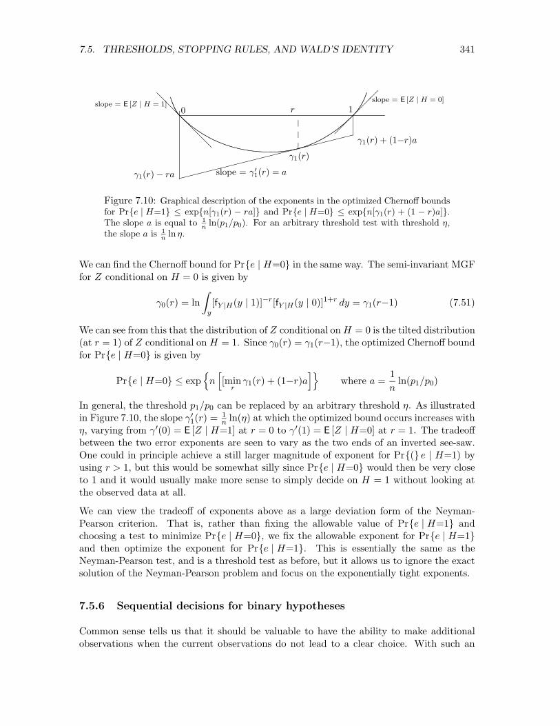
Figure 7.10: Graphical description of the exponents in the optimized Chernoff bounds for Pr{e | H=1} ≤ exp{

1 n[∞1(r) − ra]} and Pr{e | H=0} ≤ exp{n[∞1(r) + (1 − r)a]}.

The slope a is equal to n ln(p1/p0). For an arbitrary threshold test with threshold η, the slope a is n

1 ln η.

We can find the Chernoff bound for Pr{e | H=0} in the same way. The semi-invariant MGF for Z conditional on H = 0 is given by

Z ∞0(r) = ln [fY |H (y | 1)]−r[fY |H (y | 0)]1+r dy = ∞1(r−1) (7.51)

y

We can see from this that the distribution of Z conditional on H = 0 is the tilted distribution (at r = 1) of Z conditional on H = 1. Since ∞0(r) = ∞1(r−1), the optimized Chernoff bound for Pr{e | H=0} is given by

Pr{e H=0} ≤ exp n n

h[min ∞1(r) + (1−r)a

io where a =

1 ln(p1/p0)|

r n

In general, the threshold p1/p0 can be replaced by an arbitrary threshold η. As illustrated in Figure 7.10, the slope ∞1

0 (r) = n 1 ln(η) at which the optimized bound occurs increases with

η, varying from ∞0(0) = E [Z | H=1] at r = 0 to ∞0(1) = E [Z | H=0] at r = 1. The tradeoff between the two error exponents are seen to vary as the two ends of an inverted see-saw. One could in principle achieve a still larger magnitude of exponent for Pr{(} e | H=1) by using r > 1, but this would be somewhat silly since Pr{e | H=0} would then be very close to 1 and it would usually make more sense to simply decide on H = 1 without looking at the observed data at all.

We can view the tradeoff of exponents above as a large deviation form of the Neyman-Pearson criterion. That is, rather than fixing the allowable value of Pr{e | H=1} and choosing a test to minimize Pr{e | H=0}, we fix the allowable exponent for Pr{e | H=1}and then optimize the exponent for Pr{e | H=1}. This is essentially the same as the Neyman-Pearson test, and is a threshold test as before, but it allows us to ignore the exact solution of the Neyman-Pearson problem and focus on the exponentially tight exponents.

7.5.6 Sequential decisions for binary hypotheses

Common sense tells us that it should be valuable to have the ability to make additional observations when the current observations do not lead to a clear choice. With such an


ability, we have 3 possible choices at the end of each observation: choose H = 1, choose H = 0, or continue with additional observations. It is evident that we need a stopping time J to decide when to stop. We assume for the time being that stopping occurs with probability 1, both under hypothesis H = 1 and H = 0, and the indicator rv IJ=n for each n ≥ 1 is a function of Z1, . . . , Zn.

Given H = 1, the sequence of LLR’s {Sn; n ≥ 1} (where Sn = Pn Zi) is a random walk. i=1

Assume for now that the stopping rule is to stop when the random walk crosses either a threshold15 at α > 0 or a threshold at β < 0. Given H = 0, Sn =

Pin =1 Zn is also a random

walk (with a different probability measure). The same stopping rule must be used, since the decision to stop at n can be based only on Z1, . . . , Zn and not on knowledge of H. We saw that the random walk based on H = 0 uses probabilities tilted from those based on H = 1, a fact that is interesting but not necessary here.

We assume that when stopping occurs, the decision h = 0 is made if SJ ≥ α and h = 1 is made if SJ ≤ β. Given that H = 1, an error is then made if SJ ≥ α. Thus, using the probability distribution for H = 1, we apply (7.42), along with r∗ = 1, to get

Pr{e | H=1} = Pr{SJ ≥ α | H=1} ≤ exp −α (7.52)

Similarly, conditional on H = 0, an error is made if the threshold at β is crossed before that at α and the error probability is

Pr{e | H=0} = Pr{SJ ≤ β | H=0} ≤ exp β (7.53)

The error probabilities can be made as small as desired by increasing the magnitudes of α and β, but the cost of increasing α is to increase the number of observations required when H = 0. From Wald’s equality,

E [J H=0] = E [SJ | H=0] α + E [overshoot] | E [Z | H=0]

≈ E [Z | H=0]

In the approximation, we have ignored the possibility of SJ crossing the threshold at β conditional on H = 0 since this is a very small-probability event when α and β have large magnitudes. Thus we see that the expected number of observations (given H = 0) is essentially linear in α.

We next ask what has been gained quantitatively by using the sequential decision procedure here. Suppose we use a fixed-length test with n = α/E [Z | H=0]. Referring to Figure 7.10, we see that if we choose the slope a = ∞0(1), then the (exponentially tight) Chernoff bound on Pr{e | H=1} is given by e−α, but the exponent on Pr{e | H=0} is 0. In other words, by using a sequential test as described here, we simultaneously get the error exponent for

15It is unfortunate that the word ‘threshold’ has a universally accepted meaning for random walks (i.e., the meaning we are using here), and the word ‘threshold test’ has a universally accepted meaning for hypothesis testing. Stopping when Sn crosses either α or β can be viewed as an extension of an hypothesis testing threshold test in the sense that both the stopping trial and the decision is based only on the LLR, and is based on the LLR crossing either a positive or negative threshold, but the results about threshold tests in Section 7.3 are not necessarily valid for this extension.

7.5. THRESHOLDS, STOPPING RULES, AND WALD’S IDENTITY 343

H = 1 that a fixed test would provide if we gave up entirely on an error exponent for H = 0, and vice versa.16

A final question to be asked is whether any substantial improvement on this sequential decision procedure would result from letting the thresholds at α and β vary with the number of observations. Assuming that we are concerned only with the expected number of observations, the answer is no. We will not carry this argument out here, but it consists of using the Chernoff bound as a function of the number of observations. This shows that there is a typical number of observations at which most errors occur, and changes in the thresholds elsewhere can increase the error probability, but not substantially decrease it.

7.5.7 Joint distribution of crossing time and barrier

Next we look at Pr{J ≥ n, SJ ≥ α}, where again we assume that X < 0 and that ∞(r∗) = 0 for some r∗ > 0. For any r in the region where ∞(r) ≤ 0 (i.e., 0 ≤ r ≤ r∗), we have −J∞(r) ≥ −n∞(r) for J ≥ n. Thus, from the Wald identity, we have

1 ≥ E [exp[rSJ − J∞(r)] | J ≥ n, SJ ≥ α] Pr{J ≥ n, SJ ≥ α}

≥ exp[rα − n∞(r)]Pr{J ≥ n, SJ ≥ α}Pr{J ≥ n, SJ ≥ α} ≤ exp[−rα + n∞(r)] ; for r ∈ [0, r∗]. (7.54)

Since this is vaid for all r ∈ (0, r∗], we can obtain the tightest bound of this form by minimizing the right hand side of (7.54). This is the same minimization (except for the constraint r ≤ r∗) as in Figures 7.7. Assume that r∗ < r+ (i.e., that the exceptional situation17 of Figure 7.8) does not occur. Define n∗ as α/∞0(r∗). The result is then

Pr{J ≥ n, SJ ≥ α} ≤

exp [n∞(ro) − roα] for n > n∗, α/n = ∞0(ro)

(7.55)

exp [−r∗α] n ≤ n∗.

The interpretation of (7.55) is that n∗ is an estimate of the typical value of J given that the threshold at α is crossed. For n greater than this typical value, (7.55) provides a tighter bound on Pr{J ≥ n, SJ ≥ α} than the bound on Pr{SJ ≥ α} in (7.42), whereas (7.55) provides nothing new for n ≤ n∗. In Section 7.8, we shall derive the slightly stronger result that Pr

nS[Si ≥ α]

o is also upper bounded by the right hand side of (7.55).i≥n

16In the communication context, decision rules are used to detect sequentially transmitted data. The use of a sequential decision rule usually requires feedback from receiver to transmitter, and also requires a variable rate of transmission. Thus the substantial reductions in error probability are accompanied by substantial system complexity.

17The exceptional situation where ∞(r) is negative for r ≤ r+ and discontinuous at r∗ = r+, i.e., the situation in Figure 7.8), will be treated in the exercises, and is quite different from the case here. In particular, as can be seen from the figure, the optimized Chernoff bound on Pr{Sn ≥ α} is optimized at n = 1.


An almost identical upper bound to Pr{J ≤ n, SJ ≥ α} can be found (again assuming that r∗ < r+) by using the Wald identity for r > r∗. Here ∞(r) > 0, so −J∞(r) ≥ −n∞(r) for J ≤ n. The result is

Pr{J ≤ n, SJ ≥ α} ≤

exp [n∞(ro) − roα] for n < n∗, α/n = ∞0(ro)

(7.56)

exp [−r∗α] n ≥ n∗.

This strengthens the interpretation of n∗ as the typical value of J conditional on crossing the threshold at α. That is, (7.56) provides information on the lower tail of the distribution of J (conditional on SJ ≥ α), whereas (7.55) provides information on the upper tail.

7.6 Martingales

A martingale is defined as an integer-time stochastic process {Zn; n ≥ 1} with the properties that E [|Zn|] < 1 for all n ≥ 1 and

E [Zn | Zn−1, Zn−2, . . . , Z1] = Zn−1; for all n ≥ 2. (7.57)

The name martingale comes from gambling terminology where martingales refer to gambling strategies in which the amount to be bet is determined by the past history of winning or losing. If one visualizes Zn as representing the gambler’s fortune at the end of the nth

play, the definition above means, first, that the game is fair (in the sense that the expected increase in fortune from play n − 1 to n is zero), and, second, that the expected fortune on the nth play depends on the past only through the fortune on play n − 1.

The important part of the definition of a martingale, and what distinguishes martingales from other kinds of proceesses, is the form of dependence in (7.57). However, the restriction that E [|Zn|] < 1 is also important, particularly since martingales are so abstract and general that one often loses the insight to understand intuitively when this restriction is important. Students are advised to ignore this restriction when first looking at something that might be a martingale, and to check later after acquiring some understanding.

There are two interpretations of (7.57); the first and most straightforward is to view it as shorthand for E [Zn Zn−1 =zn−1, Zn−2 =zn−2, . . . , Z1 =z1] = zn−1 for all possible sample values z1, z2, . . . , zn−

|1. The second is that E [Zn Zn−1 =zn−1, . . . , Z1 =z1] is a function of

the sample values z1, . . . , zn−1 and thus E [Zn Z|

n−1, . . . , Z1] is a random variable which is a function of the random variables Z1, . . . , Z

| n−1 (and, for a martingale, a function only

of Zn−1). Students are encouraged to take the first viewpoint initially and to write out the expanded type of expression in cases of confusion. The second viewpoint, however, is very powerful, and, with experience, is the more useful viewpoint.

It is important to understand the difference between martingales and Markov chains. For the Markov chain {Xn; n ≥ 1}, each rv Xn is conditioned on the past only through Xn−1,

7.6. MARTINGALES 345

whereas for the martingale {Zn; n ≥ 1}, it is only the expected value of Zn that is conditioned on the past only through Zn−1. The rv Zn itself, conditioned on Zn−1, can also be dependent on all the earlier Zi’s. It is very surprising that so many results can be developed using such a weak form of conditioning.

In what follows, we give a number of important examples of martingales, then develop some results about martingales, and then discuss those results in the context of the examples.

7.6.1 Simple examples of martingales

Example 7.6.1 (Random walks). One example of a martingale is a zero-mean random walk, since if Zn = X1 + X2 + + Xn, where the Xi are IID and zero mean, then · · ·

E [Zn | Zn−1, . . . , Z1] = E [Xn + Zn−1 | Zn−1, . . . , Z1] (7.58) = E [Xn] + Zn−1 = Zn−1. (7.59)

Extending this example, suppose that {Xi; i ≥ 1} is an arbitrary sequence of IID random variables with mean X and let Xei = Xi − X . Then {Sn; n ≥ 1} is a random walk with Sn = X1 + + Xn and {Zn; n ≥ 1} is a martingale with Zn = X1 + + Xen. The random · · · e · · · walk and the martingale are simply related by Zn = Sn − nX, and thus general results about martingales can easily be applied to arbitrary random walks.

Example 7.6.2 (Sums of dependent zero-mean variables). Let {Xi; i ≥ 1} be a set of dependent random variables satisfying E [Xi | Xi−1, . . . ,X1] = 0. Then {Zn; n ≥ 1}, where Zn = X1 + + Xn, is a zero mean martingale. To see this, note that · · ·

E [Zn | Zn−1, . . . , Z1] = E [Xn + Zn−1 | Zn−1, . . . , Z1] = E [Xn | Xn−1, . . . ,X1] + E [Zn−1 | Zn−1, . . . , Z1] = Zn−1.

This is a more general example than it appears, since given any martingale {Zn; n ≥ 1}, we can define Xn = Zn − Zn−1 for n ≥ 2 and define X1 = Z1. Then E [Xn | Xn−1, . . . ,X1] = 0 for n ≥ 2. If the martingale is zero mean (i.e., if E [Z1] = 0), then E [X1] = 0 also.

Example 7.6.3 (Product-form martingales). Another example is a product of unit mean IID random variables. Thus if Zn = X1X2 . . .Xn, we have

E [Zn | Zn−1, . . . , Z1] = E [Xn, Zn−1 | Zn−1, . . . , Z1] = E [Xn] E [Zn−1 | Zn−1, . . . , Z1] (7.60) = E [Xn] E [Zn−1 | Zn−1] = Zn−1. (7.61)

A particularly simple case of this product example is where Xn = 2 with probability 1/2 and Xn = 0 with probability 1/2. Then

Pr{Zn = 2n} = 2−n; Pr{Zn = 0} = 1 − 2−n; E [Zn] = 1. (7.62)


Thus limn→1 Zn = 0 with probability 1, but E [Zn] = 1 for all n and limn→1 E [Zn] = 1. This is an important example to keep in mind when trying to understand why proofs about martingales are necessary and non-trivial. This type of phenomenon will be clarified somewhat by Lemma 7.8.1 when we discussed stopped martingales in Section 7.8.

An important example of a product-form martingale is as follows: let {Xi; i ≥ 1} be an IID sequence, and let {Sn = X1 + + Xn; n ≥ 1} be a random walk. Assume that the · · · semi-invariant generating function ∞(r) = ln{E [exp(rX)]} exists in some region of r around 0. For each n ≥ 1, let Zn be defined as

Zn = exp{rSn − n∞(r)} (7.63) = exp{rXn − ∞(r)} exp{rSn−1 − (n − 1)∞(r)}

= exp{rXn − ∞(r)}Zn−1. (7.64)

Taking the conditional expectation of this,

E [Zn | Zn−1, . . . , Z1] = E [exp(rXn − ∞(r))] E [Zn−1 | Zn−1, . . . , Z1] = Zn−1. (7.65)

where we have used the fact that E [exp(rXn)] = exp(∞(r)). Thus we see that {Zn; n ≥ 1}is a martingale of the product-form.

7.6.2 Scaled branching processes

A final simple example of a martingale is a “scaled down” version of a branching process {Xn; n ≥ 0}. Recall from Section 5.5 that, for each n, Xn is defined as the aggregate number of elements in generation n. Each element i of generation n, 1 ≤ i ≤ Xn has a number Yi,n

of offspring which collectively constitute generation n + 1, i.e., Xn+1 = PXn Yi,n. The rv’s i=1

Yi,n are IID over both i and n.

Let Y = E [Yi,n] be the mean number of offspring of each element of the population. Then E [Xn | Xn−1] = Y Xn−1, which resembles a martingale except for the factor of Y . We can convert this branching process into a martingale by scaling it, however. That is, define Zn = Xn/Y

n . It follows that ∑Xn

∏ Y Xn−1E [Zn | Zn−1, . . . , Z1] = E

Y | Xn−1, . . . ,X1 =

Y = Zn−1. (7.66)n n

Thus {Zn; n ≥ 1} is a martingale. We will see the surprising result later that this implies that Zn converges with probability 1 to a limiting rv as n →1.

7.6.3 Partial isolation of past and future in martingales

Recall that for a Markov chain, the states at all times greater than a given n are independent of the states at all times less than n, conditional on the state at time n. The following lemma shows that at least a small part of this independence of past and future applies to martingales.

7.7. SUBMARTINGALES AND SUPERMARTINGALES 347

Lemma 7.6.1. Let {Zn; n ≥ 1} be a martingale. Then for any n > i ≥ 1,

E [Zn | Zi, Zi−1, . . . , Z1] = Zi. (7.67)

Proof: For n = i + 1, E [Zi+1 | Zi, . . . , Z1] = Zi by the definition of a martingale. Now consider n = i + 2. Then E [Zi+2 | Zi+1, . . . , Z1] is a rv equal to Zi+1. We can view E [Zi+2 | Zi, . . . , Z1] as the conditional expectation of the rv E [Zi+2 | Zi+1, . . . , Z1] over Zi+1, conditional on Zi, . . . , Z1.

E [Zi+2|Zi, . . . , Z1] = E [E [Zi+2 | Zi+1, Zi, . . . , Z1] | Zi, . . . , Z1] = E [Zi+1 | Zi, . . . , Z1] = Zi. (7.68)

For n = i+3, (7.68), with i incremented, shows us that the rv E [Zi+3 | Zi+1, . . . , Z1] = Zi+1. Taking the conditional expectation of this rv over Zi+1 conditional on Zi, . . . , Z1, we get

E [Zi+3 | Zi, . . . , Z1] = Zi.

This argument can be applied successively to any n > i.

This lemma is particularly important for i = 1, where it says that E [Zn | Zn−1, . . . , Z1] = Z1. The left side of this is a rv which is a function (in fact the identity function) of Z1. Thus, by taking the expected value of each side, we see that

E [Zn] = E [Z1] for all n > 1. (7.69)

An important application of this is to the product form martingale in (7.65). This says that

E [exp(rSn − n∞(r)] = E [exp(rX − ∞(r))] = E [exp(rX)] /g(r) = 1. (7.70)

We will come back later to relate this to Wald’s identity.

7.7 Submartingales and supermartingales

Submartingales and supermartingales are simple generalizations of martingales that provide many useful results for very little additional work. We will subsequently derive the Kolmogorov submartingale inequality, which is a powerful generalization of the Markov inequality. We use this both to give a simple proof of the strong law of large numbers and also to better understand threshold crossing problems for random walks.

Definition 7.7.1. A submartingale is an integer-time stochastic process {Zn; n ≥ 1} that satisfies the relations

E [|Zn|] < 1 ; E [Zn | Zn−1, Zn−2, . . . , Z1] ≥ Zn−1 ; n ≥ 1. (7.71)

A supermartingale is an integer-time stochastic process {Zn; n ≥ 1} that satisfies the relations

E [|Zn|] < 1 ; E [Zn | Zn−1, Zn−2, . . . , Z1] ≤ Zn−1 ; n ≥ 1. (7.72)


In terms of our gambling analogy, a submartingale corresponds to a game that is at least fair, i.e., where the expected fortune of the gambler either increases or remains the same. A supermartingale is a process with the opposite type of inequality.18

Since a martingale satisfies both (7.71) and (7.72) with equality, a martingale is both a submartingale and a supermartingale. Note that if {Zn; n ≥ 1} is a submartingale, then {−Zn; n ≥ 1} is a supermartingale, and conversely. Thus, some of the results to follow are stated only for submartingales, with the understanding that they can be applied to supermartingales by changing signs as above.

Lemma 7.6.1, with the equality replaced by inequality, also applies to submartingales and supermartingales. That is, if {Zn; n ≥ 1} is a submartingale, then

E [Zn | Zi, Zi−1, . . . , Z1] ≥ Zi ; 1 ≤ i < n, (7.73)

and if {Zn; n ≥ 1} is a supermartingale, then

E [Zn | Zi, Zi−1, . . . , Z1] ≤ Zi ; 1 ≤ i < n. (7.74)

Equations (7.73) and (7.74) are verified in the same way as Lemma 7.6.1 (see Exercise 7.18). Similarly, the appropriate generalization of (7.69) is that if {Zn; n ≥ 1} is a submartingale, then

E [Zn] ≥ E [Zi] ; for all i, 1 ≤ i < n. (7.75)

and if {Zn; n ≥ 1} is a supermartingale, then

E [Zn] ≤ E [Zi] ; for all i, 1 ≤ i < n. (7.76)

A random walk {Sn; n ≥ 1} with Sn = X1 + + Xn is a submartingale, martingale, · · · or supermartingale respectively for X ≥ 0, X = 0, or X ≤ 0. Also, if X has a semi-invariant moment generating function ∞(r) for some given r, and if Zn is defined as Zn = exp(rSn), then the process {Zn; n ≥ 1} is a submartingale, martingale, or supermartingale respectively for ∞(r) ≥ 0, ∞(r) = 0, or ∞(r) ≤ 0. The next example gives an important way in which martingales and submartingales are related.

Example 7.7.1 (Convex functions of martingales). Figure 7.11 illustrates the graph of a convex function h of a real variable x. A function h of a real variable is defined to be convex if, for each point x1, there is a real number c with the property that h(x1) + c(x − x1) ≤ h(x) for all x.

Geometrically, this says that every tangent to h(x) lies on or below h(x). If h(x) has a derivative at x1, then c is the value of that derivative and h(x1) + c(x − x1) is the tangent line at x1. If h(x) has a discontinuous slope at x1, then there might be many choices for c; for example, h(x) = |x| is convex, and for x1 = 0, one could choose any c in the range −1 to +1.

A simple condition that implies convexity is a nonnegative second derivative everywhere. This is not necessary, however, and functions can be convex even when the first derivative

349 7.7. SUBMARTINGALES AND SUPERMARTINGALES

h(x) h(x1) + c(x − x1) c = h0(x1)

x1

Figure 7.11: Convex functions: For each x1, there is a value of c such that, for all x, h(x1) + c(x − x1) ≤ h(x). If h is differentiable at x1, then c is the derivative of h at x1.

does not exist everywhere. For example, the function ∞(r) in Figure 7.8 is convex even though it it is finite at r = r+ and infinite for all r > r+.

Jensen’s inequality states that if h is convex and X is a random variable with an expectation, then h(E [X]) ≤ E [h(X)]. To prove this, let x1 = E [X] and choose c so that h(x1) + c(x − x1) ≤ h(x). Using the random variable X in place of x and taking expected values of both sides, we get Jensen’s inequality. Note that for any particular event A, this same argument applies to X conditional on A, so that h(E [X | A]) ≤ E [h(X) | A]. Jensen’s inequality is very widely used; it is a minor miracle that we have not required it previously.

Theorem 7.7.1. Assume that h is a convex function of a real variable, that {Zn; n ≥ 1}is a martingale or submartingale, and that E [|h(Zn)|] < 1 for all n. Then {h(Zn); n ≥ 1}is a submartingale.

Proof: For any choice of z1, . . . , zn−1, we can use Jensen’s inequality with the conditioning probabilities to get

E [h(Zn)|Zn−1 =zn−1, . . . , Z1 =z1] ≥ h(E [Zn | Zn−1 =zn−1, . . . , Z1 =z1]) = h(zn−1). (7.77)

For any choice of numbers h1, . . . , hn−1 in the range of the function h, let z1, . . . , zn−1

be arbitrary numbers satisfying h(z1)=h1, . . . , h(zn−1)=hn−1. For each such choice, (7.77) holds, so that

E [h(Zn) | h(Zn−1)=hn−1, . . . , h(Z1)=h1] ≥ h(E [Zn | h(Zn−1)=hn−1, . . . , h(Z1)=h1]) = h(zn−1) = hn−1. (7.78)

completing the proof.

Some examples of this result, applied to a martingale {Zn; n ≥ 1}, are as follows:

{|Zn|; n ≥ 1} is a submartingale

{Z2 n; n ≥ 1} is a submartingale if E

£Z2

n

§ < 1

{exp(rZn); n ≥ 1} is a submartingale for r such that E [exp(rZn)] < 1.

(7.79) (7.80) (7.81)

18The easiest way to remember the difference between a submartingale and a supermartingale is to remember that it is contrary to what common sense would dictate.


A function of a real variable h(x) is defined to be concave if −h(x) is convex. It then follows from Theorem 7.7.1 that if h is concave and {Zn; n ≥ 1} is a martingale, then {h(Zn); n ≥ 1} is a supermartingale (assuming that E [|h(Zn)|] < 1). For example, if {Zn; n ≥ 1} is a positive martingale and E [| ln(Zn)|] < 1, then {ln(Zn); n ≥ 1} is a supermartingale.

7.8 Stopped processes and stopping trials

The definition of stopping trials in Section 4.5 applies to arbitrary integer-time processes {Zn; n ≥ 1} as well as to IID sequences. Recall that J is a stopping trial for a sequence {Zn; n ≥ 1} of rv’s if IJ=n is a function of Z1, . . . , Zn and if J is a rv.

If IJ=n is a function of Z1, . . . , Zn and J is a defective rv, then J is called a defective stopping trial. For some of the results to follow, it is unimportant whether J is a random variable or a defective random variable (i.e., whether or not the process stops with probability 1). If it is not specified whether J is a random variable or a defective random variable, we refer to the stopping trial as a possibly-defective stopping trial; we consider J to take on the value 1 if the process does not stop.

Definition 7.8.1. A stopped process {Z∗; n ≥ 1} for a possibly-defective stopping trial Jn

relative to a process {Zn; n ≥ 1} is the process for which Z∗ = Zn for n ≤ J and Z∗ = ZJn n for n > J .

As an example, suppose Zn models the fortune of a gambler at the completion of the nth trial of some game, and suppose the gambler then modifies the game by deciding to stop gambling under some given circumstances (i.e., at the stopping trial). Thus, after stopping, the fortune remains constant, so the stopped process models the gambler’s fortune in time, including the effect of the stopping trial.

As another example, consider a random walk with a positive and negative threshold, and consider the process to stop after reaching or crossing a threshold. The stopped process then stays at that point beyond the threshold as an artifice to simplify analysis. The use of stopped processes is similar to the artifice that we employed in Section 3.5 for first-passage times in Markov chains; recall that we added an artificial trapping state after the desired passage to simplify analysis.

We next show that the possibly-defective stopped process of a martingale is itself a martingale; the intuitive reason is that, before stopping, the stopped process is the same as the martingale, and, after stopping, Zn

∗ = Zn∗−1. The following theorem establishes this and the

corresponding results for submartingales and supermartingales.

Theorem 7.8.1. Given a stochastic process {Zn; n ≥ 1} and a possibly-defective stopping trial J for the process, the stopped process {Z∗; n ≥ 1} is a submartingale if {Zn; n ≥ 1} isn

a submartingale, is a martingale if {Zn; n ≥ 1} is a martingale, and is a supermartingale if {Zn; n ≥ 1} is a supermartingale.

351 7.8. STOPPED PROCESSES AND STOPPING TRIALS

Proof: First we show that, for all three cases, the stopped process satisfies E [ Zn∗ ] < 1

for any given n ≥ 1. Conditional on J = i for some i < n, we have Z∗ = Zi, so | |

n

E [|Z∗| | J = i] = E [|Zi| | J = i] < 1 for each i < n such that Pr{J = i} > 0.n

The reason for this is that if E [|Zi| | J = i] = 1 and Pr{J = i} > 0, then E [|Zi|] = 1, contrary to the assumption that {Zn; n ≥ 1} is a martingale, submartingale, or super-martingale. Similarly, for J ≥ n, we have Z∗ = Zn son

E [|Zn∗| | J ≥ n] = E [|Zn| | J ≥ n] < 1 if Pr{J ≥ n} > 0.

Averaging,

n−1

E [|Z∗|] = X

E [|Z∗| | J=i] Pr{J=i} + E [|Z∗| | J ≥ n] Pr{J ≥ n} < 1.n n ni=1

Next assume that {Zn; n ≥ 1} is a submartingale. For any given n > 1, consider an arbitrary initial sample sequence (Z1 = z1, Z2 = z2, . . . , Zn−1 = zn−1). Note that z1

specifies whether or not J = 1. Similarly, (z1, z2) specifies whether or not J = 2, and so forth up to (z1, . . . , zn−1), which specifies whether or not J = n − 1. Thus (z1, . . . , zn−1) specifies the sample value of J for J ≤ n − 1 and specifies that J ≥ n otherwise.

For (z1, . . . , zn−1) such that IJ≥n < n, we have zn ∗ = zn

∗−1. For all such sample values,

E £Z∗ Zn

∗−1 =zn

∗−1, ..., Z1

∗=z∗§

= z∗ (7.82)n| 1 n−1.

For the remaining case, where (z1, . . . , zn−1) is such that IJ≥n ≥ n, we have z∗ = zn. Thus n

E £Zn∗ Zn

∗−1 =zn

∗−1, ..., Z1

∗=z1 ∗§ ≥ zn

∗−1. (7.83)|

The same argument works for martingales and supermartingales by replacing the inequality in (7.83) by equality for the martingale case and the opposite inequality for the supermartingale case.

Theorem 7.8.2. Given a stochastic process {Zn; n ≥ 1} and a possibly-defective stopping trial J for the process, the stopped process {Z∗; n ≥ 1} satisfies the following conditions n

for all n ≥ 1 if {Zn; n ≥ 1} is a submartingale, martingale, or supermartingale respectively:

E [Z1] ≤ E [Zn∗] ≤ E [Zn] (submartingale) (7.84)

E [Z1] = E [Zn∗] = E [Zn] (martingale) (7.85)

E [Z1] ≥ E [Zn∗] ≥ E [Zn] (supermartingale). (7.86)

Proof: Since a process cannot stop before epoch 1, Z1 = Z1 ∗ in all cases. First consider

the case in which {Zn; n ≥ 1} is a submartingale. Theorem 7.8.1 shows that {Zn∗; n ≥ 1}

is a submartingale, and from (7.75), E [Z1] ≤ E [Z∗] for all n ≥ 1. This establishes the first n

half of (7.84) and we next prove the second half. First condition on the set of sequences for which the initial segment (z1, . . . , zi) specifies that IJ≥n = i for any given i < n. Then E [Z∗] = zi. From (7.73), E [Zn] ≥ zi, proving (7.84) for this case. For those sequences not n


having such an initial segment, Zn∗

= Zn, establishing (7.84) in that case. Averaging over these two cases gives (7.84) in general.

Finally, if {Zn; n ≥ 1} is a supermartingale, then {−Zn; n ≥ 1} is a submartingale, verifying (7.86). Since a martingale is both a submartingale and supermartingale, (7.85) follows and the proof is complete.

Consider a (non-defective) stopping trial J for a martingale {Zn; n ≥ 1}. Since the stopped process is also a martingale, we have

E [Z∗] = E [Z∗] = E [Z1] ; n ≥ 1. (7.87)n 1

Since Z∗ = ZJ for all n ≥ J and since J is finite with probability 1, we see that limn→1 Z∗ = n n ZJ with probability 1. Unfortunately, in general, E [ZJ ] is unequal to limn→1 E [Z∗] = n

E [Z1]. An example in which this occurs is the binary product martingale in (7.62). Taking the stopping trial J to be the smallest n for which Zn = 0, we have ZJ = 0 with probability 1, and thus E [ZJ ] = 0. But Zn

∗ = Zn for all n, and E [Zn∗] = 1 for all n. The problem

here is that, given that the process has not stopped by time n, Zn and Zn ∗ each have the

value 2n . Fortunately, in most situations, this type of bizarre behavior does not occur and E [ZJ ] = E [Z1]. To get a better understanding of when E [ZJ ] = E [Z1], note that for any n, we have

n

E [Zn∗] =

X E [Zn

∗ | J = i] Pr{J = i} + E [Zn ∗ | J > n] Pr{J > n} (7.88)

i=1n

= X

E [ZJ | J = i] Pr{J = i} + E [Zn | J > n] Pr{J > n} . (7.89) i=1

The left side of this equation is E [Z1] for all n. If the final term on the right converges to 0 as n →1, then the sum must converge to E [Z1]. If E [|ZJ |] < 1, then the sum also converges to E [ZJ ]. Without the condition E [|ZJ |] < 1, the sum might consist of alternating terms which converge, but whose absolute values do not converge, in which case E [ZJ ] does not exist (see Exercise 7.21 for an example). Thus we have established the following lemma.

Lemma 7.8.1. Let J be a stopping trial for a martingale {Zn; n ≥ 1}. Then E [ZJ ] = E [Z1] if and only if

lim E [Zn | J > n] Pr{J > n} = 0 and E [|ZJ |] < 1. (7.90) n→1

Example 7.8.1 (Random walks with thresholds). Recall the generating function product martingale of (7.63) in which {Zn = exp[rSn − n∞(r)]; n ≥ 1} is a martingale defined in terms of the random walk {Sn = X1+ +Xn; n ≥ 1}. From (7.85), we have E [Zn] = E [Z1], · · ·and since E [Z1] = E [exp{rX1 − ∞(r}] = 1, we have E [Zn] = 1 for all n. Also, for any possibly-defective stopping trial J , we have E [Zn

∗] = E [Z1] = 1. If J is a non-defective stopping trial, and if (7.90) holds, then

E [ZJ ] = E [exp{rSJ − J∞(r)}] = 1. (7.91)

If there are two thresholds, one at α > 0, and the other at β < 0, and the stopping rule is to stop when either threshold is crossed, then (7.91) is just the Wald identity, (7.34).

7.9. THE KOLMOGOROV INEQUALITIES 353

The nice part about the approach here is that it also applies naturally to other stopping rules. For example, for some given integer n, let Jn+ be the smallest integer i ≥ n for which Si ≥ α or Si ≤ β. Then, in the limit β → −1, Pr{SJn+ ≥ α} = Pr{∪1i=n(Si ≥ α)}. Assuming X < 0, we can find an upper bound to Pr

©SJn+ ≥ α

™ for any r > 0 and ∞(r) ≤ 0

(i.e., for 0 < r ≤ r∗) by the following steps

1 = E £exp{rSJn+ − Jn+∞(r)}

§ ≥ Pr

©SJn+ ≥ α

™ exp[rα − n∞(r)]

Pr©SJn+ ≥ α

™ ≤ exp[−rα + n∞(r)]; 0 ≤ r ≤ r∗. (7.92)

This is almost the same result as (7.54), except that it is slightly stronger; (7.54) bounded the probability that the first threshold crossing crossed α at some epoch i ≥ n, whereas this includes the possibility that Sm ≥ α and Si ≥ α for some m < n ≤ i.

7.9 The Kolmogorov inequalities

We now use the previous theorems to establish Kolmogorov’s submartingale inequality, which is a major strengthening of the Markov inequality. Just as the Markov inequality in Section 1.7 was used to derive the Chebychev inequality and then the weak law of large numbers, the Kolmogorov submartingale inequality will be used to strengthen the Chebychev inequality, from which the strong law of large numbers will follow.

Theorem 7.9.1 (Kolmogorov’s submartingale inequality). Let {Zn; n ≥ 1} be a nonnegative submartingale. Then for any positive integer m and any a > 0,

Ω æ E [Zm]

Pr max Zi ≥ a . (7.93)1≤i≤m

≤ a

Proof: Given a nonnegative submartingale {Zn; n ≥ 1}, given a > 0, and given a positive integer m, let J be the stopping trial defined as the smallest n ≤ m such that Zn ≥ a. If Zn < a for all n ≤ m, then J = m. Thus the process must stop by time m, and ZJ ≥ a if and only if Zn ≥ a for some n ≤ m. Thus

Ω æ E [ZJ ]Pr max Zn ≥ a = Pr{ZJ ≥ a} ≤ . (7.94)

1≤n≤m a

where we have used the Markov inequality. Finally, since the process must be stopped by time m, we have ZJ = Z∗ . From (7.84), E [Z∗ ] ≤ E [Zm], so the right hand side of (7.94) m m

is less than or equal to E [Zm] /a, completing the proof.

The following simple corollary shows that (7.93) takes a simpler form for nonnegative martingales.

Corollary 7.9.1 (Nonnegative martingale inequality). Let {Zn; n ≥ 1} be a nonnegative martingale. Then

Ω æ E [Z1]Pr sup Zn ≥ a ≤

a ; for all a > 0. (7.95)

n≥1


Proof For a martingale, E [Zm] = E [Z1]. Thus, from (7.93), Pr{max1≤i≤m Zi ≥ a} ≤ E[Za

1]

for all m > 1. Passing to the limit m →1 essentially yields (7.95). Exercise 7.22 illustrates why the limiting operation here is a little tricky, and shows that it is valid.

The following corollary bears the same relationship to the submartingale inequality as the Chebychev inequality does to the Markov inequality.

Corollary 7.9.2 (Kolmogorov’s martingale inequality). Let {Zn; n ≥ 1} be a martingale with E

£Z2

§ < 1 for all n ≥ 1. Thenn

Ω

1≤n≤m | | ≥ b

æ

≤ E

£

b

Z2

2 §

Pr max Znm ; for all integer m ≥ 2, all b > 0. (7.96)

Proof: Since {Zn; n ≥ 1} is a martingale and Z2 is a convex function of Zn, it follows from n Theorem 7.7.1 that {Z2; n ≥ 1} is a submartingale. Since Z2 is nonnegative, we can use n n the Kolmogorov submartingale inequality to see that

Ω æPr max ≤ E

£Z2 §

/a for any a > 0.Zn 2 ≥ a m

n≤m

Substituting b2 for a, we get (7.96).

Corollary 7.9.3 (Kolmogorov’s random walk inequality). Let {Sn; n ≥ 1} be a random walk with Sn = X1 + + Xn where {Xi; i ≥ i} is a set of IID random variables with · · · mean X and variance σ2 . Then for any positive integer m and any ≤ > 0,

Ω æ σ2

Pr max Sn − nX ≥ m≤ . (7.97)1≤n≤m

| | ≤ m≤2

Proof: {Zn = Sn − nX; n ≥ 1} is a zero mean random walk, and thus a martingale. Since E

£Z2

§ = mσ2, (7.97) follows by substituting m≤ for b in 7.96). m

Recall that the simplest form of the weak law of large numbers was given in (1.75) as Pr

©|Sm/m − X| ≥ ≤

™ ≤ σ2/(m≤2). This is strengthened in (7.97) to upper bound the

probability that any of the first m terms deviate from the mean by more than m≤. It is this strengthening that will allow us to prove the strong law of large numbers assuming only a finite variance.

The following corollary yields essentially the same result as (7.56), but is included here as another example of the use of the Kolmogorov submartingale inequality.

Corollary 7.9.4. Let {Sn; n ≥ 1} be a random walk, Sn = X1 + + Xn where each Xi· · · has mean X < 0 and semi-invariant moment generating function ∞(r). For any r > 0 such that 0 < ∞(r) < 1 (i.e., for r > r∗), and for any a > 0.

Ω æPr max Si ≥ α ≤ exp{−rα + n∞(r)}. (7.98)

1≤i≤n

Theorem 7.9.3 (SLLN). Let {Xi; i ≥ 1} be a sequence of IID random variables with mean X and standard deviation σ < 1. Let Sn = X1 + · · · + Xn. Then for any ≤ > 0,

Ω S

Pr lim n = X = 1 and (7.100) (

n

→1 n

æ

[ Slim Pr

ØØØ m −

ØØØ > ≤

)

X = 0. (7.101)n→1 m

m>n

Proof: From Section 4.2.2, (7.100) and

Ø

(7.101)

Ø

are equivalent, so we establish (7.101). As n increases, successive terms are droppped out of the union above, so the probability is

355 7.9. THE KOLMOGOROV INEQUALITIES

Proof: For r > r∗, {exp(rSn); n ≥ 1} is a submartingale. Taking a = exp(rα) in (7.93), we get (7.98).

The following theorem about supermartingales is, in a sense, the dual of the Kolmogorov submartingale inequality. Note, however, that it applies to the terms n ≥ m in the super-martingale rather than n ≤ m.

Theorem 7.9.2. Let {Zn; n ≥ 1} be a nonnegative supermartingale. Then for any positive integer m and any a > 0,

Pr [ E [Zm]

. (7.99) a

i≥m

{Zi ≥ a} ≤

Proof: For given m ≥ 1 and a > 0, let J be a possibly-defective stopping trial defined as the smallest i ≥ m for which Zi ≥ a. Let {Zn

∗; n ≥ 1} be the corresponding stopped process, which is also nonnegative and is a supermartingale from Theorem 7.8.1. For any k > m, note that Zk

∗ ≥ a iff maxm≤i≤k Zi ≥ a. Thus Ω æ

E [Zk ∗]

Pr max Zi ≥ a = Pr{Zk ∗ ≥ a} ≤ .

m≤i≤k a

Since {Zn∗; n ≥ 1} is a supermartingale, (7.76) shows that E [Z∗] ≤ E [Z∗ ]. On the other k m

hand, Z∗ = Zm since the process can not stop before epoch m. Thus Pr{maxm≤i≤k Zi ≥ a}m is at most E [Zm] /a. Since k is arbitrary, we can pass to the limit, getting (7.99) and completing the proof.

7.9.1 The strong law of large numbers (SLLN)

We now proceed to prove the strong law of large numbers assuming only a second moment. Recall that we proved the SLLN under the assumption of a finite fourth moment in Section 4.2.1. Here we use the Kolmogorov martingale inequality to show that only a second moment is required. The theorem is also true assuming only a first absolute moment, but the truncation argument we used for the weak law in Theorem 1.5.3 does not carry over simply here.


non-increasing with n. Thus we can restrict attention to n of the form 2k for integer k. For any given k, the union above can be separated into blocks as follows:

æ

[ ΩØØ ØØ [1 2[j+1

− Ø S

Pr ØØm S

X Ø > ≤ = Pr m > m

j=k

− X ≤m>2k

m m=2j +1

ΩØ Ø æ

1 2j+1

Ø Ø

ØØ

S

ØØ

Pr m X > ≤

(7.102)

æX [ ΩØØØØ

ØØØØ ≤j=k

m=2j +1

m −

2j+1

1

= X

Pr [ ©

> ≤m™

j=k

m=2j +1

|Sm − mX|

2j+1

X [ ©> ≤2j ™≤

1Pr

|Sm − mX|

(7.103)

j=k

m=2j +1

1 Ω æ

= X

Pr max Sm − mX > ≤2j

2j +1≤m≤2j+1 | |

j=k 1 Ω æX

Pr max Sm − mX > ≤2j (7.104)≤ 1≤m≤2j+1

| |j=k 1 2j+1σ2 2−k+2σ2X

= . (7.105)≤ ≤222j ≤2

j=k

In (7.102), we used the union bound on the union over j. In (7.103), we used the fact that m ≥ 2j to increase the size of the sets in the union. In (7.104), we upper bounded by adding additional terms into the maximization, and in (7.105) we used the Kolmogorov martingale inequality. The proof is completed by noting that the upper bound in (7.105) goes to 0 with increasing k.

It should be noted that, although the proof consists of a large number of steps, the steps are all quite small and familiar. Basically the proof is a slick way of upper bounding the probability of the high-order terms in a sequence by using the Kolmogorov martingale inequality, which bounds the low-order terms.

7.9.2 The martingale convergence theorem

Another famous result that follows from the Kolmogorov submartingale inequality is the martingale convergence theorem. This states that if a martingale {Zn; n ≥ 1} has the property that there is some finite M such that E [|Zn|] ≤ M for all n, then limn→1 Zn

exists (and is finite) with probability 1. This is a powerful theorem in more advanced work, but it is not quite as useful as it appears, since the restriction E [|Zn|] ≤ M is more than a technical restriction; for example it is not satisfied by a zero-mean random walk. We prove the theorem with the additional restriction that there is some finite M such that E

£Z2

§ ≤ M for all n.n

357 7.10. MARKOV MODULATED RANDOM WALKS

Theorem 7.9.4 (Martingale convergence theorem). n

§Let ≤{ZM

n; n ≥ 1} be a martingale and assume that there is some finite M such that E

£Z2 for all n. Then there

is a random variable Z such that, for all sample sequences except a set of probability 0, limn→1 Zn = Z.

Proof∗: From Theorem 7.7.1 and the assumption that E £Zn

2§ ≤ M , {Zn

2; n ≥ 1} is a submartingale. Thus, from (7.75), E

£Z2

§ is nondecreasing in n, and since E

£Z2

§ is

bounded, limn→1 E £Zn

2§

= M 0 for some Mn0 ≤ M . For any integer k, the process {Y

n

n = Zk+n − Zk; n ≥ 1} is a zero mean martingale (see Exercise 7.29). Thus from Kolmogorov’s martingale inequality,

Ω æPr max ≤ E

£(Zk+m − Zk)2

§ /b2 . (7.106)

1≤n≤m |Zk+n − Zk| ≥ b

Next, observe that E [Zk+mZk | Zk = zk, Zk−1 = zk−1, . . . , Z1 = z1] = zk2 , and therefore,

E [Zk+mZk] = E £Zk

2§. Thus E

£(Zk+m − Zk)2

§ = E

£Zk

2+m

§ − E

£Zk

2§ ≤ M 0 − E

£Zk

2§. Since

this is independent of m, we can pass to the limit, obtaining

Pr sup Zk+n − Zkk . (7.107)

Ω

n≥1 | | ≥ b

æ

≤ M 0 −

b

E 2

£Z2

§

Since limk→1 E £Z2

§ = M 0, we then have, for all b > 0,k

Ω ælim Pr sup |Zk+n − Zk| ≥ b = 0. (7.108)

k→1 n≥1

This means that with probability 1, a sample sequence of {Zn; n ≥ 1} is a Cauchy sequence, and thus approaches a limit, concluding the proof.

This result can be relatively easily interpreted for branching processes. For a branching process {Xn; n ≥ 1} where Y is the expected number of offspring of an individual, {Xn/Y

n; n ≥ 1} is a martingale that satisfies the above conditions. If Y ≤ 1, the branching process dies out with probability 1, so Xn/Y

n approaches 0 with probability 1. For Y > 1, however, the branching process dies out with some probability less than 1 and approaches 1 otherwise. Thus, the limiting random variable Z is 0 with the probability that the process ultimately dies out, and is positive otherwise. In the latter case, for large n, the interpretation is that when the population is very large, a law of large numbers effect controls its growth in each successive generation, so that Xn/Y

n tends to change in a random way for small n, and then changes increasingly little as n increases.

7.10 Markov modulated random walks

Frequently it is useful to generalize random walks to allow some dependence between the variables being summed. The particular form of dependence here is the same as the Markov reward processes of Section 3.5. The treatment in Section 3.5 discussed only expected


rewards, whereas the treatment here focuses on the random variables themselves. Let {Ym; m ≥ 0} be a sequence of (possibly dependent) rv’s, and let

n−1 {Sn; n ≥ 1} where Sn =

XYm. (7.109)

m=0

be the process of successive sums of these random variables. Let {Xn; n ≥ 0} be a Markov chain, and assume that each Yn can depend on Xn and Xn+1. Conditional on Xn and Xn+1, however, Yn is independent of Yn−1, . . . , Y1, and of Xi for all i =6 n, n−1. Assume that Yn, conditional on Xn and Xn+1 has a distribution function Fij (y) = Pr{Yn ≤ y | Xn = i,Xn+1 = j}. Thus each rv Yn depends only on the associated transition in the Markov chain, and this dependence is the same for all n.

The process {Sn; n ≥ 1} is called a Markov modulated random walk. If each Ym is positive, it is also the sequence of epochs in a semi-Markov process. For each m, Ym is associated with the transition in the Markov chain from time m to m + 1, and Sn is the aggregate reward up to but not including time n. Let Y ij denote E [Yn | Xn = i,Xn+1 = j] and Y i denote E [Yn | Xn = i]. Let {Pij } be the set of transition probabilities for the Markov chain, so Y i =

PPijY ij . We may think of the process {Yn; n ≥ 0} as evolving along with the j

Markov chain. The distributions of the variables Yn are associated with the transitions from Xn to Xn+1, but the Yn are otherwise independent random variables.

In order to define a martingale related to the process {Sn; n ≥ 1}, we must subtract the mean reward from {Sn} and must also compensate for the effect of the state of the Markov chain. The appropriate compensation factor turns out to be the relative-gain vector defined in Section 3.5.

For simplicity, consider only finite-state irreducible Markov chains with M states. Let π = (π1, . . . , πM) be the steady-state probability vector for the chain, let Y = (Y 1, . . . , Y M)T

be the vector of expected rewards, let g = πY be the steady-state gain per unit time, and let w = (w1, . . . , wM)T be the relative-gain vector. From Theorem 3.5.1, w is the unique solution to

w + ge = Y + [P ]w ; w1 = 0. (7.110)

We assume a fixed starting state X0 = k. As we now show, the process Zn; n ≥ 1 given by

Zn = Sn − ng + wXn − wk ; n ≥ 1 (7.111)

is a martingale. First condition on a given state, Xn−1 = i.

E [Zn | Zn−1, Zn−2, . . . , Z1,Xn−1 = i] . (7.112)

Since Sn = Sn−1 + Yn−1, we can express Zn as

Zn = Zn−1 + Yn−1 − g + wXn − wXn−1 . (7.113)

Since E [Yn−1 | Xn−1 = i] = Y i and E [wXn | Xn−1 = i] = P

j Pij wj , we have

E [Zn Zn−1, Zn−2, . . . , Z1,Xn−1 = i] = Zn−1 + Y i − g + X

Pij wj − wi. (7.114)| j


From (7.110) the final four terms in (7.114) sum to 0, so

E [Zn | Zn−1, . . . , Z1,Xn−1 = i] = Zn−1. (7.115)

Since this is valid for all choices of Xn−1, we have E [Zn | Zn−1, . . . , Z1] = Zn−1. Since the expected values of all the reward variables Y i exist, we see that E [|Yn|] < 1, so that E [|Zn|] < 1 also. This verifies that {Zn; n ≥ 1} is a martingale. It can be verified similarly that E [Z1] = 0, so E [Zn] = 0 for all n ≥ 1.

In showing that {Zn; n ≥ 1} is a martingale, we actually showed something a little stronger. That is, (7.115) is conditioned on Xn−1 as well as Zn−1, . . . , Z1. In the same way, it follows that for all n > 1,

E [Zn | Zn−1,Xn−1, Zn−2,Xn−2, . . . , Z1,X1] = Zn−1. (7.116)

In terms of the gambling analogy, this says that {Zn; n ≥ 1} is fair for each possible past sequence of states. A martingale {Zn; n ≥ 1} with this property (i.e., satisfying (7.116)) is said to be a martingale relative to the joint process {Zn,Xn; n ≥ 1}. We will use this martingale later to discuss threshold crossing problems for Markov modulated random walks. We shall see that the added property of being a martingale relative to {Zn,Xn}gives us added flexibility in defining stopping times.

As an added bonus to this example, note that if {Xn; n ≥ 0} is taken as the embedded chain of a Markov process (or semi-Markov process), and if Yn is taken as the time interval from transition n to n + 1, then Sn becomes the epoch of the nth transition in the process.

7.10.1 Generating functions for Markov random walks

Consider the same Markov chain and reward variables as in the previous example, and assume that for each pair of states, i, j, the moment generating function

gij (r) = E [exp(rYn) | Xn = i,Xn+1 = j] . (7.117)

exists over some open interval (r−, r+) containing 0. Let [Γ(r)] be the matrix with terms Pij gij (r). Since [Γ(r)] is an irreducible nonnegative matrix, Theorem 3.4.1 shows that [Γ(r)] has a largest real eigenvalue, ρ(r) > 0, and an associated positive right eigenvector, ∫(r) = (∫1(r), . . . , ∫M(r))T that is unique within a scale factor. We now show that the process {Mn(r); n ≥ 1} defined by

exp(rSn)∫Xn (r)Mn(r) = ρ(r)n∫k(r)

. (7.118)

is a product type Martingale for each r ∈ (r−, r+). Since Sn = Sn−1 + Yn−1, we can express Mn(r) as

exp(rYn−1) ∫Xn (r)Mn(r) = Mn−1(r) ρ(r)∫Xn−1 (r)

. (7.119)


The expected value of the ratio in (7.119), conditional on Xn−1 = i, is ∑exp(rYn 1)∫Xn (r)

∏ Pj Pij gij (r)∫j (r)

E − | Xn 1 =i = = 1. (7.120) ρ(r)∫i(r)

−ρ(r)∫i(r)

where, in the last step, we have used the fact that ∫(r) is an eigenvector of [Γ(r)]. Thus, E [Mn(r) | Mn 1(r), . . . ,M1(r),Xn 1 = i] = M− − n−1(r). Since this is true for all choices of i, the condition on Xn−1 = i can be removed and {Mn(r); n ≥ 1} is a martingale. Also, for n > 1,

E [Mn(r) | Mn−1(r),Xn−1, . . . ,M1(r),X1] = Mn−1(r). (7.121)

so that {Mn(r); n ≥ 1} is also a martingale relative to the joint process {Mn(r),Xn; n ≥ 1}.

It can be verified by the same argument as in (7.120) that E [M1(r)] = 1. It then follows that E [Mn(r)] = 1 for all n ≥ 1.

One of the uses of this martingale is to provide exponential upper bounds, similar to (7.18), to the probabilities of threshold crossings for Markov modulated random walks. Define

Mn(r) = exp(rSn)minj (∫j (r)) . (7.122)f

ρ(r)n∫k(r)

Then f (r) ≤ Mn

hMn(r)

i ≤ 1. For any µ > 0, the Markov inequality can be Mn (r), so E f

applied to f (r) to get Mn

PrnMn(r) ≥ µ

o 1 E

hMn(r)

i 1 . (7.123)f ≤

µ f ≤

µ

For any given α, and any given r, 0 ≤ r < r+, we can choose µ = exp(rα)ρ(r)−n minj (∫j (r))/∫k(r), and for r > 0. Combining (7.122) and (7.123),

Pr{Sn ≥ α} ≤ ρ(r)n exp(−rα)∫k(r)/ min(∫j (r)). (7.124)j

This can be optimized over r to get the tightest bound in the same way as (7.18).

7.10.2 stopping trials for martingales relative to a process

A martingale {Zn; n ≥ 1} relative to a joint process {Zn,Xn; n ≥ 1} was defined as a martingale for which (7.116) is satisfied, i.e., E [Zn | Zn−1,Xn−1, . . . , Z1,X1] = Zn−1. In the same way, we can define a submartingale or supermartingale {Zn; n ≥ 1} relative to a joint process {Zn,Xn; n ≥ 1} as a submartingale or supermartingale satisfying (7.116) with the = sign replaced by ≥ or ≤ respectively. The purpose of this added complication is to make it easier to define useful stopping rules.

As generalized in Definition 4.5.2, a generalized stopping trial IJ≥n for a sequence of pairs of rv’s (Z1,X1), (Z2,X2) . . . , is a positive integer-valued rv such that, for each n ≥ 1, I{J=n}is a function of Z1,X1, Z2,X2, . . . , Zn,Xn.


Theorems 7.8.1, 7.8.2 and Lemma 7.8.1 all carry over to martingales (submartingales or supermartingales) relative to a joint process. These theorems are stated more precisely in Exercises 7.23 to 7.26. To summarize them here, assume that {Zn; n ≥ 1} is a martingale (submartingale or supermartingale) relative to a joint process {Zn,Xn; n ≥ 1} and assume that J is a stopping trial for {Zn; n ≥ 1} relative to {Zn,Xn; n ≤ 1}. Then the stopped process is a martingale (submartingale or supermartingale) respectively, (7.84 — 7.86) are satisfied, and, for a martingale, E [ZJ ] = E [Z1] is satisfied iff (7.90) is satisfied.

7.10.3 Markov modulated random walks with thresholds

We have now developed two martingales for Markov modulated random walks, both conditioned on a fixed initial state X0 = k. The first, given in (7.111), is {Zn = Sn − ng + wXn − wk; n ≥ 1}. Recall that E [Zn] = 0 for all n ≥ 1 for this martingale. Given two thresholds, α > 0 and β < 0, define J as the smallest n for which Sn ≥ α or Sn ≤ β. The indicator function IJ=n of {J = n}, is 1 iff β < Si < α for 1 ≤ i ≤ n − 1 and either Sn ≥ α or Sn ≤ β. Since Si = Zi + ig − wXi + wk, Si is a function of Zi and Xi, so the stopping trial is a function of both Zi and Xi for 1 ≤ i ≤ n. It follows that J is a stopping trial for {Zn; n ≥ 1}relative to {Zn,Xn; n ≥ 1}. From Lemma 7.8.1, we can assert that E [ZJ ] = E [Z1] = 0 if (7.90) is satisfied, i.e., if limn→1 E [Zn | J > n] Pr{J > n} = 0 is satisfied. Using the same argument as in Lemma 7.5.1, we can see that Pr{J > n} goes to 0 at least geometrically in n. Conditional on J > n, β < Sn < α, so Sn is bounded independent of n. Also wXn is bounded, since the chain is finite state, and ng is linear in n. Thus E [Zn | J > n] varies at most linearly with n, so (7.90) is satisfied, and

0 = E [ZJ ] = E [SJ ] − E [J ] g + E [wXn ] − wk. (7.125)

Recall that Wald’s equality for random walks is E [SJ ] = E [J ] X. For Markov modulated random walks, this is modified, as shown in (7.125), by the relative-gain vector terms.

The same arguments can be applied to the generating function martingale of (7.118). Again, let J be the smallest n for which Sn ≥ α or Sn ≤ β. As before, Si is a function of Mi(r) and Xi, so In is a function of Mi(r) and Xi for 1 ≤ i ≤ n − 1. It follows that J is a stopping trial for {Mn(r); n ≥ 1} relative to {Mn(r),Xn; n ≥ 1} Next we need the following lemma:

Lemma 7.10.1. For the martingale {Mn(r); n ≥ 1} relative to {Mn(r),Xn; n ≥ 1} defined in (7.118), where {Xn; n ≥ 0} is a finite-state Markov chain, and for the above stopping trial J ,

lim E [Mn(r) J > n] Pr{J > n} = 0. (7.126) n→1

|

Proof: From lemma 4, slightly modified for the case here, there is a δ > 0 such that for all states i, j, and all n > 1 such that Pr{J = n,Xn−1 = i,Xn = j} > 0,

E [exp(rSn | J = n,Xn−1 = i,Xn = j] ≥ δ. (7.127)

Since the stopped process, {M∗(r); n ≥ 1}, is a martingale, we have for each m,n

m

1 = E [M∗ (r)] ≥ X E [exp(rS

ρ(n

r

))∫nX

∫n

k

((r

r

))| J = n]

. (7.128)mn=1


From (7.127), we see that there is some δ0 > 0 such that

E [exp(rSn)∫Xn (r)] /∫k(r) | J = n] ≥ δ0

for all n such that Pr{J = n} > 0. Thus (7.128) is bounded by

1 ≥ δ0 X

ρ(r)nPr{J = n} . n≤m

Since this is valid for all m, it follows by the argument in the proof of theorem 7.5.1 that limn→1 ρ(r)nPr{J > n} = 0. This, along with (7.127), establishes (7.126), completing the proof.

From Lemma 7.8.1, we have the desired result: ∑exp(rSJ )∫XJ (r)

∏

E [MJ (r)] = E [ρ(r)]J ∫k(r)

= 1; r− < r < r+. (7.129)

This is the extension of the Wald identity to Markov modulated random walks, and is used in the same way as the Wald identity. As shown in Exercise 7.28, the derivative of (7.129), evaluated at r = 0, is the same as (7.125).

7.11 Summary

Each term in a random walk {Sn; n ≥ 1} is a sum of IID random variables, and thus the study of random walks is closely related to that of sums of IID variables. The focus in random walks, however, as in most of the processes we have studied, is more in the relationship between the terms (such as which term first crosses a threshold) than in the individual terms. We started by showing that random walks are a generalization of renewal processes, are central to studying the queueing delay for G/G/1 queues, and to sequential analysis for hypothesis testing.

A major focus of the chapter was on estimating the probabilities of very unlikely events, a topic known as large deviation theory. We started by studying the Chernoff bound to Pr{Sn ≥ α} for α > 0 and E [X] < 0. We then developed the Wald identity, which can be used to find tight upper bounds to the probability that a threshold is ever crossed by a random walk. One of the insights gained here was that if a threshold at α is crossed, it is likely to be crossed at a time close to n∗ = α/∞0(r∗), where r∗ is the positive root of ∞(r). We also found that r∗ plays a fundamental role in the probability of threshold crossings. For questions of typical behavior, the mean and variance of a random variable are the major quantities of interest, but when interested in atypically large deviations, r∗ is the major parameter of interest.

We next introduced martingales, submartingales and supermartingales. These are sometimes regarded as somewhat exotic topics in mathematics, but in fact they are very useful in a large variety of relatively simple processes. For example, we showed that all of the random walk issues of earlier sections can be treated as a special case of martingales, and

363 7.11. SUMMARY

that martingales can be used to model both sums and products of random variables. We also showed how Markov modulated random walks can be treated as martingales.

Stopping trials, as first introduced in chapter 4, were then applied to martingales. We defined a stopped process {Z∗; n ≥ 1} to be the same as the original process {Znn

up to the stopping point, and then constant thereafter. Theorems 7.8.1 and 7.8.2 showed ; n ≥ 1}

that the stopped process has the same form (martingale, submartingale, or supermartingale) as the original process, and that the expected values E [Zn

∗] are between E [Z1] and E [Zn]. We also looked at E [ZJ ] and found that it is equal to E [Z1] iff (7.90) is satisfied. The Wald identity can be viewed as E [ZJ ] = E [Z1] = 1 for the Wald martingale, Zn = exp{rSn − n∞(r)}. We then found a similar identity for Markov modulated random walks. In deriving results for Markov modulated random walks, it was necessary to define martingales relative to other processes in order to find suitable stopping trials, also defined on martingales relative to other processes. This added restriction on martingales is useful in other contexts.

The Kolmogorov inequalities were next developed. They are analogs of the Markov inequality and Chebyshev inequality, except they bound initial segments of submartingales and martingales rather than single rv’s. They were used, first, to prove the SLLN with only a second moment and, second,the martingale convergence theorem.

A standard reference on random walks, and particularly on the analysis of overshoots is [Fel66]. Dembo and Zeitouni, [5] develop large deviation theory in a much more general and detailed way than the introduction here. The classic reference on martingales is [6], but [4] and [16] are more accessible.


7.12 Exercises

Exercise 7.1. Consider the simple random walk {Sn; n ≥ 1} of Section 7.1.1 with Sn = X1 + · · · + Xn and Pr{Xi = 1} = p; Pr{Xi = −1} = 1 − p; assume that p ≤ 1/2.

a) Show that Prn k

n 1 {Sn k≥ ≥ }o

= hPr

n n≥1 {Sn ≥ 1} for any positive integer k.

Hint: Given that the random walk ever reaches the value 1,

o

i

consider a new random walk

S S

starting at that time and explore the probability that the new walk ever reaches a value 1 greater than its starting point.

b) Find a quadratic equation for y = PrnS

n≥1 {Sn ≥ 1}o . Hint: explore each of the two

possibilities immediately after the first trial.

c) For p < 1/2, show that the two roots of this quadratic equation are p/(1 − p) and 1. Argue that Pr

nS n≥1 {Sn ≥ 1}

o cannot be 1 and thus must be p/(1 − p).

d) For p = 1/2, show that the quadratic equation in part c) has a double root at 1, and

thus PrnS

n≥1 {Sn ≥ 1}o

= 1. Note: this is the very peculiar case explained in the section

on Wald’s equality.

e) For p < 1/2, show that p/(1 − p) = exp(−r∗) where r∗ is the unique positive root of g(r) = 1 where g(r) = E

£erX

§.

Exercise 7.2. Consider a G/G/1 queue with IID arrivals {Xi; i ≥ 1}, IID FCFS service times {Yi; i ≥ 0}, and an initial arrival to an empty system at time 0. Define Ui = Xi −Yi−1

for i ≥ 1. Consider a sample path where (u1, . . . , u6) = (1, −2, 2, −1, 3, −2).

a) Let Zi 6 = U6 + U6−1 + . . . + U6−i+1. Find the queueing delay for customer 6 as the max

imum of the ‘backward’ random walk with elements 0, Z16, Z2

6, . . . , Z66; sketch this random

walk.

b) Find the queueing delay for customers 1 to 5.

c) Which customers start a busy period (i.e., arrive when the queue and server are both empty)? Verify that if Zi

6 maximizes the random walk in part a), then a busy period starts with arrival 6 − i.

d) Now consider a forward random walk Vn = U1 + +Un. Sketch this walk for the sample · · ·path above and show that the queueing delay for each customer is the difference between two appropriately chosen values of this walk.

Exercise 7.3. A G/G/1 queue has a deterministic service time of 2 and interarrival times that are 3 with probability p and 1 with probability 1 − p.

a) Find the distribution of W1, the wait in queue of the first arrival after the beginning of a busy period.

b) Find the distribution of W , the steady-state wait in queue. 1

365 7.12. EXERCISES

c) Repeat parts a) and b) assuming the service times and interarrival times are exponentially distributed with rates µ and ∏ respectively.

Exercise 7.4. A sales executive hears that one of his sales people is routing half of his incoming sales to a competitor. In particular, arriving sales are known to be Poisson at rate one per hour. According to the report (which we view as hypothesis 1), each second arrival is routed to the competition; thus under hypothesis 1 the interarrival density for successful sales is f(y|H1) = ye−y; y ≥ 0. The alternate hypothesis (H0) is that the rumor is false and the interarrival density for successful sales is f(y|H0) = e−y; y ≥ 0. Assume that, a priori, the hypotheses are equally likely. The executive, a recent student of stochastic processes, explores various alternatives for choosing between the hypotheses; he can only observe the times of successful sales however.

a) Starting with a successful sale at time 0, let Si be the arrival time of the ith subsequent successful sale. The executive observes S1, S2, . . . , Sn(n ≥ 1) and chooses the maximum aposteriori probability hypothesis given this data. Find the joint probability density f(S1, S2, . . . , Sn|H1) and f(S1, . . . , Sn|H0) and give the decision rule.

b) This is the same as part a) except that the system is in steady state at time 0 (rather than starting with a successful sale). Find the density of S1 (the time of the first arrival after time 0) conditional on H0 and on H1. What is the decision rule now after observing S1, . . . , Sn.

c) This is the same as part b), except rather than observing n successful sales, the successful sales up to some given time t are observed. Find the probability, under each hypothesis, that the first successful sale occurs in (s1, s1 + ∆], the second in (s2, s2 + ∆], . . . , and the last in (sN(t), sN(t) + ∆] (assume ∆ very small). What is the decision rule now?

Exercise 7.5. For the hypothesis testing problem of Section 7.3, assume that there is a cost C0 of choosing H1 when H0 is correct, and a cost C1 of choosing H0 when H1 is correct. Show that a threshold test minimizes the expected cost using the threshold η = (C1p1)/(C0p0).

Exercise 7.6. Consider a binary hypothesis testing problem where H is 0 or 1 and a one dimensional observation Y is given by Y = H + U where U is uniformly distributed over [-1, 1] and is independent of H.

a) Find fY |H (y | 0), fY |H (y | 1) and the likelihood ratio Λ(y).

b) Find the threshold test at η for each η, 0 < η < 1 and evaluate the conditional error probabilities, q0(η) and q1(η).

c) Find the error curve u(α) and explain carefully how u(0) and u(1/2) are found (hint: u(0) = 1/2).

d) Describe a decision rule for which the error probability under each hypothesis is 1/4. You need not use a randomized rule, but you need to handle the don’t-care cases under the threshold test carefully.


Exercise 7.7. a) For given α, 0 < α ≤ 1, let η∗ achieve the supremum sup0 q (η) + ≤η<1 1

η(q0(η) − α). Show that η∗ ≤ 1/α. Hint: Think in terms of Lemma 7.3.1 applied to a very simple test.

b) Show that the magnitude of the slope of the error curve u(α) at α is at most 1/α.

Exercise 7.8. Define ∞(r) as ln [g(r)] where g(r) = E [exp(rX)]. Assume that X is discrete with possible outcomes {ai; i ≥ 1}, let pi denote Pr{X = ai}, and assume that g(r) exists in some open interval (r , r+) containing r = 0. For any given r, r < r < r+, define a − −random variable Xr with the same set of possible outcomes {ai; i ≥ 1} as X, but with a probability mass function qi = Pr{Xr = ai} = pi exp[air − ∞(r)]. Xr is not a function of X, and is not even to be viewed as in the same probability space as X; it is of interest simply because of the behavior of its defined probability mass function. It is called a tilted random variable relative to X, and this exercise, along with Exercise 7.9 will justify our interest in it.

a) Verify that P

i qi = 1.

b) Verify that E [Xr] = P

i aiqi is equal to ∞0(r). 2c) Verify that Var [Xr] =

Pi ai qi − (E [Xr])2 is equal to ∞00(r).

d) Argue that ∞00(r) ≥ 0 for all r such that g(r) exists, and that ∞00(r) > 0 if ∞00(0) > 0.

e) Give a similar definition of Xr for a random variable X with a density, and modify parts a) to d) accordingly.

Exercise 7.9. Assume that X is discrete, with possible values {ai; i ≥ 1) and probabilities Pr{X = ai} = pi. Let Xr be the corresponding tilted random variable as defined in Exercise 7.8. Let Sn = X1 + + Xn be the sum of n IID rv’s with the distribution of X, and let · · · Sn,r = X1,r + + Xn,r be the sum of n IID tilted rv’s with the distribution of Xr. Assume · · · that X < 0 and that r > 0 is such that ∞(r) exists.

a) Show that Pr{Sn,r =s} = Pr{Sn =s} exp[sr − n∞(r)]. Hint: first show that

Pr{X1,r =v1, . . . ,Xn,r =vn} = Pr{X1 =v1, . . . ,Xn =vn} exp[sr − n∞(r)]

where s = v1 + + vn.· · ·

b) Find the mean and variance of Sn,r in terms of ∞(r).

c) Define a = ∞0(r) and σr 2 = ∞00(r). Show that Pr

©|Sn,r − na| ≤

√2nσr

™ > 1/2. Use this

to show that

Prn| Sn − na |≤

√2nσr

o > (1/2) exp[−r(an +

√2n σr) + n∞(r)].

d) Use this to show that for any ≤ and for all sufficiently large n,

Pr©Sn ≥ n(∞0(r) − ≤)

™ >

1 exp[−rn(∞0(r) + ≤) + n∞(r)].

2

d) Evaluate your expression when X has an exponential density, fX (x) = a1e−∏x for x ≥ 0 and fX (x) = a2eµx for x < 0 and where a1 and a2 are chosen so that X = 0.

Exercise 7.13. A random walk {Sn; n ≥ 1}, with S n n = Xi , has the i=1 following

probability density for Xi

P

e−x ;

f (x) =

e−e−1 −1 ≤ x ≤ 1

X

= 0 ; elsewhere.

a) Find the values of r for which g(r) = E [exp(rX)] = 1.

b) Let Pα be the probability that the random walk ever crosses a threshold at α for some α > 0. Find an upper bound to Pα of the form Pα ≤ e−αA where A is a constant that does not depend on α; evaluate A.

367 7.12. EXERCISES

Exercise 7.10. Consider a random walk with thresholds α > 0, β < 0. We wish to find Pr{SJ ≥ α} in the absence of a lower threshold. Use the upper bound in (7.42) for the probability that the random walk crosses α before β.

a) Given that the random walk crosses β first, find an upper bound to the probability that α is now crossed before a yet lower threshold at 2β is crossed.

b) Given that 2β is crossed before α, upperbound the probability that α is crossed before a threshold at 3β. Extending this argument to successively lower thresholds, find an upper bound to each successive term, and find an upper bound on the overall probability that α is crossed. By observing that β is arbitrary, show that (7.42) is valid with no lower threshold.

Exercise 7.11. This exercise verifies that Corollary 7.5.1 holds in the situation where ∞(r) < 0 for all r ∈ (r−, r+) and where r∗ is taken to be r+ (see Figure 7.7).

a) Show that for the situation above, exp(rSJ ) ≤ exp(rSJ − J∞(r)) for all r ∈ (0, r∗).

b) Show that E [exp(rSJ )] ≤ 1 for all r ∈ (0, r∗).

c) Show that Pr{SJ ≥ α} ≤ exp(−rα) for all r ∈ (0, r∗). Hint: Follow the steps of the proof of Corollary 7.5.1.

d) Show that Pr{SJ ≥ α} ≤ exp(−r∗α).

Exercise 7.12. a) Use Wald’s equality to show that if X = 0, then E [SJ ] = 0 where J is the time of threshold crossing with one threshold at α > 0 and another at β < 0.

b) Obtain an expression for Pr{SJ ≥ α}. Your expression should involve the expected value of SJ conditional on crossing the individual thresholds (you need not try to calculate these expected values).

c) Evaluate your expression for the case of a simple random walk.


c) Find a lower bound to Pα of the form Pα ≥ Be−αA where A is the same as in part b) and B is a constant that does not depend on α. Hinto find an elaborate bound. Also recall that E the random walk and g(r∗) = 1.

£ t: keep§ it simple — you are not expected er∗SJ = 1 where J is a stopping trial for

Exercise 7.14. Let {Xn; n ≥ 1} be a sequence of IID integer valued random variables with the probability mass function PX (k) = Qk. Assume that Qk > 0 for k ≤ 10 and

= 0 for k > 10. Let {Sn; n ≥ 1} be a random walk with Sn = | |

LetQk | | X1 + · · · + Xn. α > 0 and β < 0 be integer valued thresholds, let J be the smallest value of n for which either Sn ≥ α or Sn ≤ β. Let {Sn

∗; n ≥ 1} be the stopped random walk; i.e., S∗ = Sn forn n ≤ J and Sn

∗ = SJ for n > J . Let πi ∗ = Pr{SJ = i}.

a) Consider a Markov chain in which this stopped random walk is run repeatedly until the point of stopping. That is, the Markov chain transition probabilities are given by Pij = Qj−i

for β < i < α and Pi0 = 1 for i ≤ β and i ≥ α. All other transition probabilities are 0 and the set of states is the set of integers [−9 + β, 9 + α]. Show that this Markov chain is ergodic.

b) Let {πi} be the set of steady-state probabilities for this Markov chain. Find the set of probabilities {πi

∗} for the stopping states of the stopped random walk in terms of {πi}.

c) Find E [SJ ] and E [J ] in terms of {πi}.

Exercise 7.15. a) Conditional on H0 for the hypothesis testing problem, consider the random variables Zi = ln[f(Yi|H1)/f(Yi|H0)]. Show that r∗, the positive solution to g(r) = 1, where g(r) = E [exp(rZi)], is given by r∗ = 1.

b) Assuming that Y is a discrete random variable (under each hypothesis), show that the tilted random variable Zr with r = 1 has the PMF PY (y|H1).

Exercise 7.16. a) Suppose {Zn; n ≥ 1} is a martingale. Verify (7.69); i.e., E [Zn] = E [Z1] for n > 1.

b) If {Zn; n ≥ 1} is a submartingale, verify (7.75), and if a supermartingale, verify (7.76).

Exercise 7.17. Suppose {Zn; n ≥ 1} is a martingale. Show that

E £Zm Zni , Zni−1 , . . . , Zn1

§ = Zni for all 0 < n1 < n2 < . . . < ni < m. |

Exercise 7.18. a) Assume that {Zn; n ≥ 1} is a submartingale. Show that

E [Zm | Zn, Zn−1, . . . , Z1] ≥ Zn for all n < m.

b) Show that

E £Zm Zni , Zni−1 , . . . , Zn1

§ ≥ Zni for all 0 < n1 < n2 < . . . < ni < m. |

c) Assume now that {Zn; n ≥ 1} is a supermartingale. Show that parts a) and b) still hold with ≥ replaced by ≤.

369 7.12. EXERCISES

Exercise 7.19. Let {Zn = exp[rSn − n∞(r)]; n ≥ 1} be the generating function martingale of (7.63) where Sn = X1 + + Xn and X1, . . .Xn are IID with mean X < 0. Let J be · · · the possibly-defective stopping trial for which the process stops after crossing a threshold at α > 0 (there is no negative threshold). Show that exp[r∗α] is an upper bound to the probability of threshold crossing by considering the stopped process {Zn

∗; n ≥ 1}.

The purpose of this exercise is to illustrate that the stopped process can yield useful upper bounds even when the stopping trial is defective.

Exercise 7.20. This problem uses martingales to find the expected number of trials E [J ] before a fixed pattern, a1, a2, . . . , ak, of binary digits occurs within a sequence of IID binary random variables X1,X2, . . . (see Exercises 4.32 and 3.28 for alternate approaches). A mythical casino and set of gamblers who follow a prescribed strategy will be used to determine E [J ]. The casino has a game where, on the ith trial, gamblers bet money on either 1 or 0. After bets are placed, Xi above is used to select the outcome 0 or 1. Let p(1) = pX (1) and p(0) = 1 − p(1) = pX (0). If an amount s is bet on 1, the casino receives s if Xi = 0, and pays out s/p(1) − s (plus returning the bet s) if Xi = 1. If s is bet on 0, the casino receives s if Xi = 1, and pays out s/p(0) − s (plus the bet s) if Xi = 0.

a) Assume an arbitrary pattern of bets by various gamblers on various trials (some gamblers might bet arbitrary amounts on 0 and some on 1 at any given trial). Let Yi be the net gain of the casino on trial i. Show that E [Yi] = 0 (i.e., show that the game is fair). Let Zn = Y1 + Y2 + + Yn be the aggregate gain of the casino over n trials. Show that for the · · · given pattern of bets, {Zn; n ≥ 1} is a martingale.

b) In order to determine E [J ] for a given pattern a1, a2, . . . , ak, we program our gamblers to bet as follows:

i) Gambler 1 has an initial capital of 1 which is bet on a1 at trial 1. If he wins, his capital grows to 1/p(a1), which is bet on a2 at trial 2. If he wins again, he bets his entire capital, 1/[p(a1)p(a2)], on a3 at trial 3. He continues, at each trial i, to bet his entire capital on ai until he loses at some trial (in which case he leaves with no money) or he wins on k successive trials (in which case he leaves with 1/[p(a1) . . . p(ak)].

ii) Gambler j, j > 1, follows exactly the same strategy but starts at trial j. Note that if the pattern a1, . . . , ak appears for the first time at J = n, then gambler n − k + 1 leaves at time n with capital 1/[p(a1) . . . p(ak)] and gamblers j < n − k + 1 all lose their capital.

Suppose the string (a1, . . . , ak) is (0, 1). Let for the above gambling strategy. Given that J = 3 (i.e., that X2 = 0 and X3 = 1), note that gambler 1 loses his money at either trial 1 or 2, gambler 2 leaves at time 3 with 1/[p(0)p(1)] and gambler 3 loses his money at time 3. Show that ZJ = 3 − 1/[p(0)p(1)] given J = 3. Find ZJ given J = n for arbitrary n ≥ 2 (note that the condition J = n uniquely specifies ZJ ).

c) Find E [ZJ ] from part a). Use this plus part b) to find E [J ].

d) Repeat parts b) and c) using the string (a1, . . . , ak) = (1, 1). Be careful about gambler 3 for J = 3. Show that E [J ] = 1/[p(1)p(1)] + 1/p(1)

e) Repeat parts b) and c) for (a1, . . . , ak) = (1, 1, 1, 0, 1, 1).


Exercise 7.21. a) This exercise shows why the condition E [|ZJ |] < 1 is required in Lemma 7.8.1. Let Z1 = −2 and, for n ≥ 1, let Zn+1 = Zn[1 + Xn(3n + 1)/(n + 1)] where X1,X2, . . . are IID and take on the values +1 and −1 with probability 1/2 each. Show that {Zn; n ≥ 1} is a martingale.

b) Consider the stopping trial J such that J is the smallest value of n > 1 for which Zn and Zn−1 have the same sign. Show that, conditional on n < J , Zn = (−2)n/n and, conditional on n = J , ZJ = −(−2)n(n − 2)/(n2 − n).

c) Show that E [|ZJ |] is infinite, so that E [ZJ ] does not exist according to the definition of expectation, and show that limn→1 E [Zn|J > n] Pr{J > n} = 0.

Exercise 7.22. This exercise shows why the sup of a martingale can behave markedly differently from the maximum of an arbitrarily large number of the variables. More precisly, it shows that Pr

©supn≥1 Zn ≥ a

™ can be unequal to Pr

nS n≥1{Zn ≥ a}

o .

a) Consider a martingale where Zn can take on only the values 2−n−1 and 1 − 2−n−1, each with probability 1/2. Given that Zn, conditional on Zn−1, is independent of Z1, . . . Zn−2, find Pr{Zn|Zn−1} for each n so that the martingale condition is satisfied.

b) Show that Pr©supn≥1 Zn ≥ 1

™ = 1/2 and show that Pr{

S n{Zn ≥ 1}} = 0.

Z1c Show that for every ≤ > 0, Pr©supn≥1 Zn ≥ a

™ ≤ a−≤ . Hint: Use the relationship between

Pr©supn≥1 Zn ≥ a

™ and Pr{

S n{Zn ≥ a}} while getting around the issue in part b).

d Use part c) to establish (7.95).

Exercise 7.23. Show that Theorem 7.7.1 is also valid for martingales relative to a joint process. That is, show that if h is a convex function of a real variable and if {Zn; n ≥ 1}is a martingale relative to a joint process {Zn,Xn; n ≥ 1}, then {h(Zn); n ≥ 1} is a submartingale relative to {h(Zn),Xn; n ≥ 1}.

Exercise 7.24. Show that if {Zn; n ≥ 1} is a martingale (submartingale or supermartingale) relative to a joint process {Zn,Xn; n ≥ 1} and if J is a stopping trial for {Zn; n ≥ 1}relative to {Zn,Xn; n ≥ 1}, then the stopped process is a martingale (submartingale or supermartingale) respectively relative to the joint process.

Exercise 7.25. Show that if {Zn; n ≥ 1} is a martingale (submartingale or supermartingale) relative to a joint process {Zn,Xn; n ≥ 1} and if J is a stopping trial for {Zn; n ≥ 1}relative to {Zn,Xn; n ≥ 1}, then the stopped process satisfies (7.84), (7.85), or (7.86) respectively.

Exercise 7.26. Show that if {Zn; n1} is a martingale relative to a joint process {Zn,Xn; n ≥1} and if J is a stopping trial for {Zn; n ≥ 1} relative to {Zn,Xn; n ≥ 1}, then E [ZJ ] = E [Z1] if and only f (7.90) is satisfied.

371 7.12. EXERCISES

Exercise 7.27. Consider the Markov modulated random walk in the figure below. The random variables Yn in this example take on only a single value for each transition, that value being 1 for all transitions from state 1, 10 for all transitions from state 2, and 0 otherwise. ≤ > 0 is a very small number, say ≤ < 10−6 .

1 − ≤ ✘✿ 1♥②

≤ ③ 0♥♥②

1/2 ③ 2

1 − ≤ ②♥

1/2 ≤

a) Show that the steady-state gain per transition is 5.5/(1+ ≤). Show that the relative-gain vector is w = (0, (≤ − 4.5)/[≤(1 + ≤)], (10≤ + 4.5)/[≤(1 + ≤)]).

b) Let Sn = Y0 +Y1 + +Yn−1 and take the starting state X0 to be 0. Let J be the smallest· · ·value of n for which Sn ≥ 100. Find Pr{J = 11} and Pr{J = 101}. Find an estimate of E [J ] that is exact in the limit ≤ 0.→

c) Show that Pr{XJ = 1} = (1 − 45≤ + o(≤))/2 and that Pr{XJ = 2} = (1 + 45≤ + o(≤))/2. Verify, to first order in ≤ that (7.125) is satisfied.

Exercise 7.28. Show that (7.125) results from taking the derivative of (7.129) and evaluating it at r = 0.

Exercise 7.29. Let {Zn; n ≥ 1} be a martingale, and for some integer m, let Yn = Zn+m −Zm.

a) Show that E [Yn | Zn+m−1 = zn+m−1, Zn+m−2 = zn+m−2, . . . , Zm = zm, . . . , Z1 = z1] = zn+m−1 − zm.

b) Show that E [Yn | Yn−1 = yn−1, . . . , Y1 = y1] = yn−1

c) Show that E [|Yn|] < 1. Note that b) and c) show that {Yn; n ≥ 1} is a martingale.

Exercise 7.30. a) Show that Theorem 7.7.1 is valid if {Zn; n ≥ 1} is a submartingale rather than a martingale. Hint: Simply follow the proof of Theorem 7.7.1 in the text.

b) Show that the Kolmogorov martingale inequality also holds if {Zn; n ≥ 1} is a sub-martingale rather than a martingale.

Exercise 7.31 (Continuation of continuous-time branching). This exercse views the continuous-time branching process of Exercise 6.15 as a stopped random walk. Recall that the process was specified there as a Markov process such that for each state j, j ≥ 0, the transition rate to j + 1 is j∏ and to j − 1 is jµ. There are no other transitions, and in particular, there are no transitions out of state 0, so that the Markov process is reducible. Recall that the embedded Markov chain is the same as the embedded chain of an M/M/1 queue except that there is no transition from state 0 to state 1.

a) To model the possible extinction of the population, convert the embedded Markov chain abve to a stopped random walk, {Sn; n ≥ 0. The stopped random walk starts at S0 =


0 and stops on reaching a threshold at −1. Before stopping, it moves up by one with probability ∏

∏+µ and downward by 1 with probability µ ∏+µ at each step. Give the (verysimple) relationship between the state Xn of the Markov chain and the state Sn of the stopped random walk for each n ≥ 0.

b) Find the probability that the population eventually dies out as a function of ∏ and µ. Be sure to consider all three cases ∏ > µ, ∏ < µ, and ∏ = µ.

MIT OpenCourseWarehttp://ocw.mit.edu

6.262 Discrete Stochastic Processes Spring 2011

For information about citing these materials or our Terms of Use, visit: http://ocw.mit.edu/terms.

http://ocw.mit.edu

http://ocw.mit.edu/terms

Discrete Stochastic Processes, Chapter 7: Random Walks, Large Deviations, and ... · RANDOM WALKS,...

Documents

Transcript of Discrete Stochastic Processes, Chapter 7: Random Walks, Large Deviations, and ... · RANDOM WALKS,...