Discrete Random Variables and Probability Distributions

Random Variables

• Random Variable (RV): A numeric outcome that results from an experiment

• For each element of an experiment’s sample space, the random variable can take on exactly one value

• Discrete Random Variable: An RV that can take on only a finite or countably infinite set of outcomes

• Continuous Random Variable: An RV that can take on any value along a continuum (but may be reported “discretely”

• Random Variables are denoted by upper case letters (Y)• Individual outcomes for RV are denoted by lower case

letters (y)

Probability Distributions

• Probability Distribution: Table, Graph, or Formula that describes values a random variable can take on, and its corresponding probability (discrete RV) or density (continuous RV)

• Discrete Probability Distribution: Assigns probabilities (masses) to the individual outcomes

• Continuous Probability Distribution: Assigns density at individual points, probability of ranges can be obtained by integrating density function

• Discrete Probabilities denoted by: p(y) = P(Y=y)• Continuous Densities denoted by: f(y)• Cumulative Distribution Function: F(y) = P(Y≤y)

Discrete Probability Distributions

yyF

FF

ypbYPbF

yYPyF

yp

yyp

yYPyp

b

y

y

in increasinglly monotonica is )(

1)(0)(

)()()(

)()(

:(CDF)Function on Distributi Cumulative

1)(

0)(

)()(

:Function (Mass)y Probabilit

all

Example – Rolling 2 Dice (Red/Green)

Red\Green 1 2 3 4 5 6

1 2 3 4 5 6 72 3 4 5 6 7 83 4 5 6 7 8 94 5 6 7 8 9 105 6 7 8 9 10 116 7 8 9 10 11 12

Y = Sum of the up faces of the two die. Table gives value of y for all elements in S

Rolling 2 Dice – Probability Mass Function & CDF

y p(y) F(y)

2 1/36 1/36

3 2/36 3/36

4 3/36 6/36

5 4/36 10/36

6 5/36 15/36

7 6/36 21/36

8 5/36 26/36

9 4/36 30/36

10 3/36 33/36

11 2/36 35/36

12 1/36 36/36

y

t

tpyF

yyp

2

)()(

inresult can die 2 waysof #

tosumcan die 2 waysof #)(

Rolling 2 Dice – Probability Mass FunctionDice Rolling Probability Function

0

0.02

0.04

0.06

0.08

0.1

0.12

0.14

0.16

0.18

2 3 4 5 6 7 8 9 10 11 12

y

p(y

)

Rolling 2 Dice – Cumulative Distribution FunctionDice Rolling - CDF

0

0.1

0.2

0.3

0.4

0.5

0.6

0.7

0.8

0.9

1

1 2 3 4 5 6 7 8 9 10 11 12 13

y

F(y

)

Expected Values of Discrete RV’s

• Mean (aka Expected Value) – Long-Run average value an RV (or function of RV) will take on

• Variance – Average squared deviation between a realization of an RV (or function of RV) and its mean

• Standard Deviation – Positive Square Root of Variance (in same units as the data)

• Notation:– Mean: E(Y) = – Variance: V(Y) = 2

– Standard Deviation:

Expected Values of Discrete RV’s

2

2222

all

2

all all

2

all

22

all

2

222

all

all

:Deviation Standard

)1()(2

)()(2)(

)(2)()(

)())(()( :Variance

)()()( :)(function a ofMean

)()( :Mean

YEYE

ypyypypy

ypyyypy

YEYEYEYV

ypygYgEYg

yypYE

yyy

yy

y

y

Expected Values of Linear Functions of Discrete RV’s

a

aypya

ypyaypaay

ypbabaybaYV

baypbyypa

ypbaybaYE

babaYYg

baY

y

yy

y

yy

y

22

all

22

all

22

all

2

all

2

all all

all

)()(

)()(

)()()(][

)()(

)()(][

)constants ,()( :FunctionsLinear

Example – Rolling 2 Dice

y p(y) yp(y) y2p(y)

2 1/36 2/36 4/36

3 2/36 6/36 18/36

4 3/36 12/36 48/36

5 4/36 20/36 100/36

6 5/36 30/36 180/36

7 6/36 42/36 294/36

8 5/36 40/36 320/36

9 4/36 36/36 324/36

10 3/36 30/36 300/36

11 2/36 22/36 242/36

12 1/36 12/36 144/36

Sum 36/36=1.00

252/36=7.00

1974/36=54.833

4152.28333.5

8333.5)0.7(8333.54

)(

0.7)()(

2

212

2

2222

12

2

y

y

ypyYE

yypYE

Tchebysheff’s Theorem/Empirical Rule

• Tchebysheff: Suppose Y is any random variable with mean and standard deviation . Then: P(-k≤ Y ≤ +k) ≥ 1-(1/k2) for k ≥ 1– k=1: P(-1≤ Y ≤ +1) ≥ 1-(1/12) = 0 (trivial result)– k=2: P(-2≤ Y ≤ +2) ≥ 1-(1/22) = ¾– k=3: P(-3≤ Y ≤ +3) ≥ 1-(1/32) = 8/9

• Note that this is a very conservative bound, but that it works for any distribution

• Empirical Rule (Mound Shaped Distributions)– k=1: P(-1≤ Y ≤ +1) 0.68– k=2: P(-2≤ Y ≤ +2) 0.95– k=3: P(-3≤ Y ≤ +3) 1

Proof of Tchebysheff’s Theorem

2222

2

22

22222

22)(

)(

2222

222

222

)(

2)(

)(

2)(

2

22

11)()(1

1

)(1

)()(

)()()()(

)( : )Region In

)( : )Region In

)()()()()()(

)()()(

:Variance of definition theof use Making

),)[())](),[()])(()

:parts 3 into line real Breaking

kkYkPkYkP

kk

kYkPk

kYPkkYPk

kYPkypykYPk

kykyiii

kykyi

ypyypyypy

ypyYV

kμiiikμμ-kiiμ-k,- i

kμ

μ-k

kμ

kμ

μ-k

μ-k

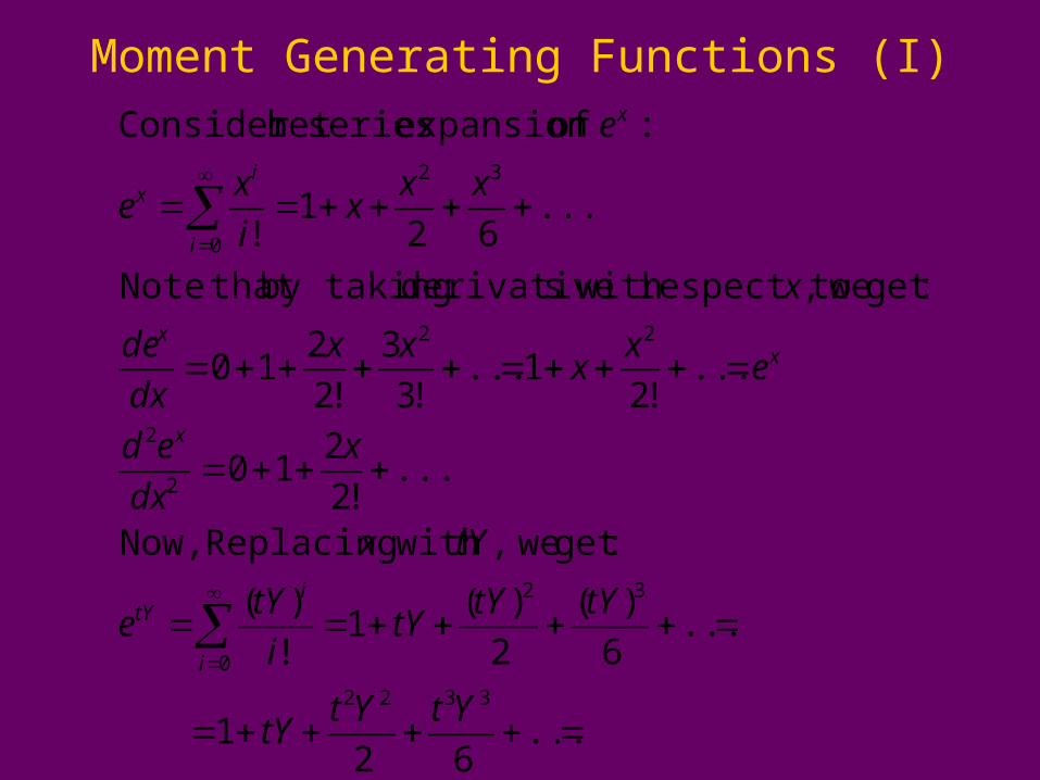
Moment Generating Functions (I)

...62

1

...6

)(

2

)(1

!

)(

:get we, with Replacing Now,

...!2

210

...!2

1...!3

3

!2

210

:get we, respect to with sderivative by taking that Note

...62

1!

: ofexpansion series heConsider t

3322

32

0

2

2

22

32

0

YtYttY

tYtYtY

i

tYe

tYx

x

dx

ed

ex

xxx

dx

de

x

xxx

i

xe

e

i

itY

x

xx

i

ix

x

Moment Generating Functions (II)

K

t

k

tt

y i

i

y

tytY

tY

tt

tY

ttt

tY

YEtMYEtMYEtM

ypi

tyypeeEtM

tMe

YYtYYdt

ed

YYYt

tYYYttY

Ydt

de

tt

0

)(2

00

all 0 all

22

0

32

0

2

2

0

322

0

322

0

)(...,)(''),()('

)(!

)()(

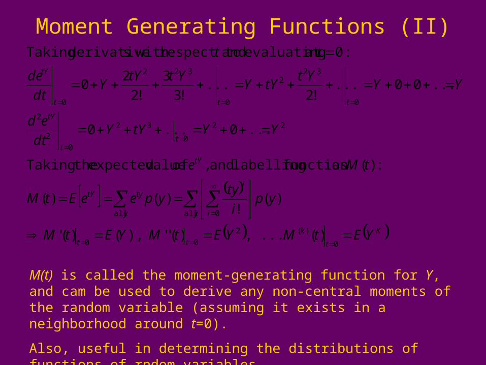
:)( asfunction labelling and , of valueexpected theTaking

...0...0

...00...!2

...!3

3

!2

20

:0at evaluating and respect to with sderivative Taking

M(t) is called the moment-generating function for Y, and cam be used to derive any non-central moments of the random variable (assuming it exists in a neighborhood around t=0).

Also, useful in determining the distributions of functions of rndom variables

Probability Generating Functions

))1()...(1()(

)1()(''

)()('

:)(Let

))1()...(1(

)1(

:sderivative its and function heConsider t

1

)(

1

1

22

2

1

kYYYEtP

YYEtP

YEtP

tEtP

tkYYYdt

td

tYYdt

td

Ytdt

dt

t

t

k

t

t

Y

kYk

Yk

YY

YY

Y

P(t) is the probability generating function for Y

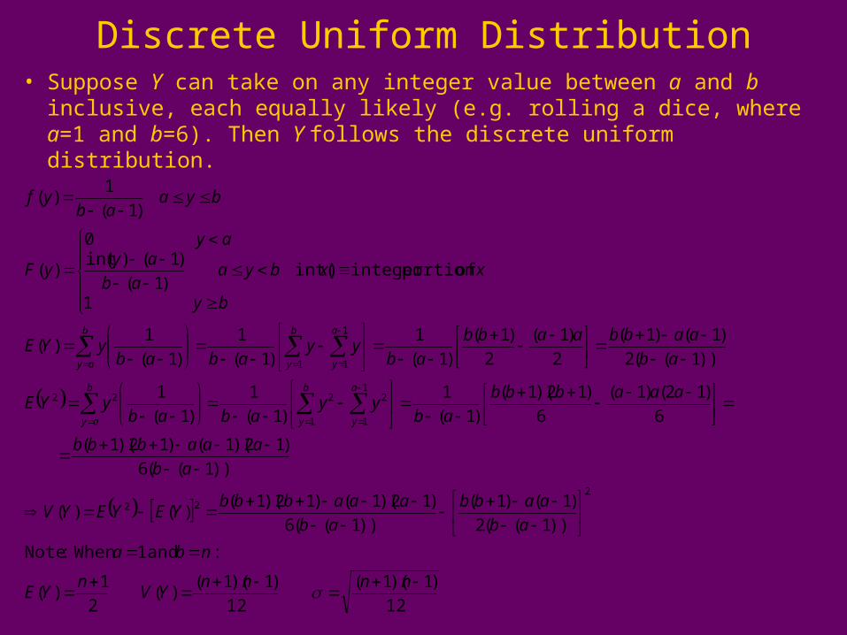
Discrete Uniform Distribution• Suppose Y can take on any integer value between a and b

inclusive, each equally likely (e.g. rolling a dice, where a=1 and b=6). Then Y follows the discrete uniform distribution.

12

)1)(1(

12

)1)(1()(

2

1)(

: and 1 When :Note

))1((2

)1()1(

))1((6

)12)(1()12)(1()()(

))1((6

)12)(1()12)(1(

6

)12()1(

6

)12)(1(

)1(

1

)1(

1

)1(

1

))1((2

)1()1(

2

)1(

2

)1(

)1(

1

)1(

1

)1(

1)(

1

ofportion integer )int()1(

)1()(int0

)(

)1(

1)(

2

22

1

1

2

1

222

1

11

nnnnYV

nYE

nba

ab

aabb

ab

aaabbbYEYEYV

ab

aaabbb

aaabbb

abyy

ababyYE

ab

aabbaabb

abyy

ababyYE

by

xxbyaab

ayay

yF

byaab

yf

b

ay

a

y

b

y

b

ay

a

y

b

y

Bernoulli Distribution• An experiment consists of one trial. It can result in one of

2 outcomes: Success or Failure (or a characteristic being Present or Absent).

• Probability of Success is p (0<p<1)• Y = 1 if Success (Characteristic Present), 0 if not

)1(

)1()()(

1)1(0

1)1(0)()(

01

1)(

222

222

1

0

pp

ppppYEYEYV

pppYE

pppyypYE

yp

ypyp

y

Binomial Experiment

• Experiment consists of a series of n identical trials• Each trial can end in one of 2 outcomes: Success or

Failure• Trials are independent (outcome of one has no

bearing on outcomes of others)• Probability of Success, p, is constant for all trials• Random Variable Y, is the number of Successes in

the n trials is said to follow Binomial Distribution with parameters n and p

• Y can take on the values y=0,1,…,n• Notation: Y~Bin(n,p)

Binomial Distribution

onDistributiy Probabilit "Legitimate" 1)1()1()(

)( :Expansion Binomial

)1,,,BINOMDIST( :functionby obtained is )(

)0,,,BINOMDIST( :functionby obtained is )(

:Functions EXCEL

,...,1,0)1()()()3

)1( ) )( (and oft arrangemeneach ofy Probabilit )2

)!(!

! positions of sequence ain ) )( (and arranging of waysof # 1)

:GeneralIn

)1()0()0()(0

)1(3)1()1()(1,,

)1(3)2()2()(2,,

)3()3()(3

:Trials 3 with experimentan of outcomesConsider

0 0

0

3

2

2

3

nn

y

n

y

yny

n

i

inin

yny

ynyss

ss

ppppy

nyp

bai

nba

pnyyF

pnyyp

nyppy

nypyYP

ppFynSy

yny

n

y

nnFynSy

ppYPFFFPyFFF

pppYPFFSFSFSFFPyFFSFSFSFF

pppYPFSSSFSSSFPyFSSSFSSSF

ppYPSSSPySSS

Binomial Distribution (n=10,p=0.10)

0

0.05

0.1

0.15

0.2

0.25

0.3

0.35

0.4

0.45

0.5

0 1 2 3 4 5 6 7 8 9 10

y

p(y

)

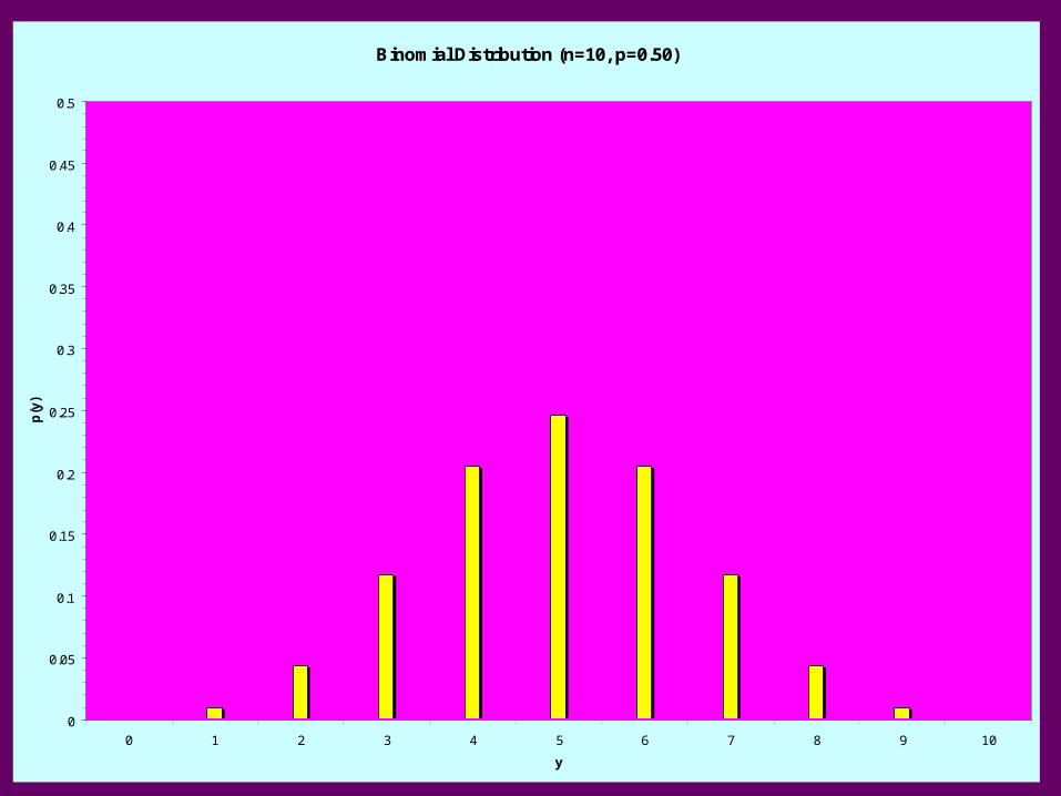
Binomial Distribution (n=10, p=0.50)

0

0.05

0.1

0.15

0.2

0.25

0.3

0.35

0.4

0.45

0.5

0 1 2 3 4 5 6 7 8 9 10

y

p(y

)

Binomial Distribution(n=10,p=0.8)

0

0.05

0.1

0.15

0.2

0.25

0.3

0.35

0 1 2 3 4 5 6 7 8 9 10

y

p(y

)

Binomial Distribution – Expected Value

npnpppnpqpnp

qpyny

nnpqp

yny

nnYE

nynyyyyy

qpyny

nqp

ynyy

ynYE

y

qpyny

nyqp

yny

nyYE

pqnyqpyny

nyf

nn

n

y

ynyn

y

yny

n

y

ynyn

y

yny

n

y

ynyn

y

yny

yny

)1()1()(

!)1(!

)!1(

!)1(!

)!1()(

1,...,0,...,1 :Note 11Let

)!()!1(

!

)!()!1(

!)(

)0 when 0(Summand

)!(!

!

)!(!

!)(

1,...,1,0)!(!

!)(

11

1

0*

*)1(***

1

0*

)1*(1***

***

11

10

Binomial Distribution – Variance and S.D.

)1(

)1()()1()()(

)1(]1)1[()1()()1(

)1()1()1()()1(

!)2(!

)!2()1(

!)2(!

)!2)(1()1(

2,...,0,...,2 :Note 22Let

)!()!2(

!)1(

)1,0 when 0(Summand

)!(!

!)1(

)!(!

!)1()1(

:not is )()1(but get, toe?)(impossibldifficult is :Note

1,...,1,0)!(!

!)(

22222

2222222

22222

2

0**

**)2(*****

22

0**

)2**(2******

******

2

20

22

pnp

pnpnppnppnYEYEYV

pnppnnpnppnpnnpnppnnYEYYEYE

pnnpppnnqppnn

qpyny

npnnqp

yny

nnnYYE

nynyyyyy

qpyny

nYYE

y

qpyny

nyyqp

yny

nyyYYE

YEYEYYEYE

pqnyqpyny

nyf

nn

n

y

ynyn

y

yny

n

y

yny

n

y

ynyn

y

yny

yny

Binomial Distribution – MGF & PGF

nn

y

yny

n

y

ynyyY

nn

n

tntttnt

tnttnt

ntn

y

ynyt

n

y

ynytytY

pptppty

n

ppy

nttEtP

pnp

pnpnppnppnYEYEYV

pnppnnpnppnpnnp

pppppnnpMYE

npppnpMYE

eppeepeppennptM

eppenppeppentM

ppeppey

n

ppy

neeEtM

)1()1(

)1()(

)1(

)1()()1()()(

)1(1)1(

]1[)1()1()1()1()1()1()1()0(''

)1()1()1()0(')(

)1()1()1()(''

)1()1()('

)1()1(

)1()(

0

0

22222

22222

122

1

12

11

0

0

Geometric Distribution

• Used to model the number of Bernoulli trials needed until the first Success occurs (P(S)=p)– First Success on Trial 1 S, y = 1 p(1)=p – First Success on Trial 2 FS, y = 2 p(2)=(1-p)p – First Success on Trial k F…FS, y = k p(k)=(1-p)k-1 p

1)1(1

1)1()(

,...1,0,...2,1 that noting and 1 Setting

)1()1()(

,...2,1)1()(

0*

*

1

**

1

1

1

1

1

1

p

p

ppppyp

yyyy

ppppyp

yppyp

y

y

y

y

y

y

y

y

y

Geometric Distribution - Expectations

2

222

2

2

22

2222

2333

22

2

1

12

2

12

2

12

2

1

1

222

1

1

111

1

11212)()(

2)1(212)()1(

22

1

2)1()1(2

)1(

1

1

)1()1(

1

)1(

)1(

)1(

)1()1)(1(

1

)(

p

q

p

q

p

p

p

p

pp

pYEYEYV

p

p

p

pp

pp

qYEYYEYE

p

q

p

pq

q

pqqpq

qdq

dpq

q

q

dq

dpq

qqdq

dpqq

dq

dpq

dq

qdpqpqyyYYE

pp

p

q

qqp

q

qqp

q

q

dq

dp

qqdq

dpq

dq

dp

dq

dqppqyYE

y

y

y

y

y

y

y

y

y

y

y

y

y

y

y

y

Geometric Distribution – MGF & PGF

tp

pt

tq

pttq

q

ptq

tqq

pqt

q

ppqttEtP

ep

pe

qe

peqe

q

pqe

qeq

pqe

q

ppqeeEtM

y

y

y

y

y

yy

y

yyY

t

t

t

t

y

ytt

y

yt

y

yty

y

ytytY

)1(11

)(

)1(11

)(

1

1

111

1

1

1

111

1

Negative Binomial Distribution

• Used to model the number of trials needed until the rth Success (extension of Geometric distribution)

• Based on there being r-1 Successes in first y-1 trials, followed by a Success

5)Chapter in Given (Proof )1(

)(

5)Chapter in Given (Proof )(

,...1,)1(1

1)(

2p

prYV

p

rYE

rryppr

yyp ryr

Poisson Distribution

• Distribution often used to model the number of incidences of some characteristic in time or space:– Arrivals of customers in a queue– Numbers of flaws in a roll of fabric– Number of typos per page of text.

• Distribution obtained as follows:– Break down the “area” into many small “pieces” (n pieces)– Each “piece” can have only 0 or 1 occurrences (p=P(1))– Let =np ≡ Average number of occurrences over “area”– Y ≡ # occurrences in “area” is sum of 0s & 1s over “pieces”– Y ~ Bin(n,p) with p = /n– Take limit of Binomial Distribution as n with p = /n

Poisson Distribution - Derivation

)1,,POISSON( :)(

)0,,POISSON( :)(

:Functions EXCEL

onDistributiy Probabilit "Legitimate" 1!!

)(

! :function lexponentia ofexpansion Series

,...2,1,0!!

)(lim

1lim :get weCalculus, From

1lim!

)(lim

fixed allfor 11

lim...lim :Note

11

...1

lim!

1)(

)1)...(1(lim

!

1)!(

)!)(1)...(1(lim

!1

)!(!

!lim)(lim

: aslimit Taking

1)!(!

!)1(

)!(!

!)(

000

0

yyF

yyp

eey

ey

eyp

i

xe

yy

ee

yyp

en

a

nyyp

yn

yn

n

n

nn

yn

n

n

n

n

ynn

ynnn

y

n

n

nynn

ynynnn

ynnyny

nyp

n

nnyny

npp

yny

nyp

y

y

y

y

y

x

ix

yy

n

an

n

n

n

y

n

nn

n

n

yn

yn

y

yn

yn

yyny

nn

ynyyny

Poisson Distribution - Expectations

2222

22

22

2

22

220

1

1

110

][)()(

)()1(

)!2(

)!2(!)1(

!)1()1(

)!1()!1(!!)(

,...2,1,0!

)(

YEYEYV

YEYYEYE

eey

e

y

e

y

eyy

y

eyyYYE

eey

ey

e

y

ey

y

eyYE

yy

eyf

y

y

y

y

y

y

y

y

y

y

y

y

y

y

y

y

y

Poisson Distribution – MGF & PGF

)1(

0

00

1

0

00

!

!!)(

!

!!)(

tt

y

y

y

y

y

yyY

ee

y

yt

y

yt

y

ytytY

eeey

te

y

te

y

ettEtP

eeey

ee

y

ee

y

eeeEtM

tt

Hypergeometric Distribution• Finite population generalization of Binomial Distribution• Population:

– N Elements– k Successes (elements with characteristic if interest)

• Sample:– n Elements– Y = # of Successes in sample (y = 0,1,,,,,min(n,k)

5)Chapter in (Proof 1

)(

5)Chapter in (Proof )(

),min(,...,1,0)(

N

nN

N

kN

N

knYV

N

knYE

kny

n

N

yn

kN

y

k

yp