Discrete Optimization - Heuristics - SINTEF 1 Geir Hasle - eVITA Winter School 2009 Discrete...
239
1 ICT Geir Hasle - eVITA Winter School 2009 Discrete Optimization - Heuristics Geir Hasle SINTEF ICT, Applied Mathematics, Oslo, Norway University of Jyväskylä, Finland eVITA Winter School 2009 Geilo, January 11.-16. 2009
-
Upload
truongkhuong -
Category
Documents
-
view
220 -
download
1
Transcript of Discrete Optimization - Heuristics - SINTEF 1 Geir Hasle - eVITA Winter School 2009 Discrete...
1ICT
Geir Hasle - eVITA Winter School 2009
Discrete Optimization - Heuristics
Geir HasleSINTEF ICT, Applied Mathematics, Oslo, Norway
University of Jyväskylä, Finland
eVITA Winter School 2009Geilo, January 11.-16. 2009
2ICT
Geir Hasle - eVITA Winter School 2009
Summary (slide 1)
Discrete optimization problems are importantDiscrete optimization problems are often computationally hardExact methods may take too long, will give guaranteesBetter to find a good solution to the real problem than the optimal problem to an overly idealized problemLocal Search is a robust, simple and fast methodLocal Search gives few and weak guaranteesLocal Search is local, gets trapped in a local optimum
3ICT
Geir Hasle - eVITA Winter School 2009
Summary (slide 2)Metaheuristics move on from local optima and explorelarger parts of the solution spaceMetaheuristics are often based on local searchDifferent strategies, many variantsThere is no free lunchThis area is a lot of fun, many challengesShort road from theoretical to practical improvements
4ICT
Geir Hasle - eVITA Winter School 2009
Outline
2-slide talk (thanks, François!)Background and MotivationDefinition of Discrete Optimization Problems (DOP) Basic conceptsLocal SearchMetaheuristicsGUT No free lunchFuture directionsSummary

5ICT
Geir Hasle - eVITA Winter School 2009
LiteratureH. H. Hoos, T. Stützle: Stochastic Local Search - Foundations and Applications, ISBN 1-55860-872-9. Elsevier 2005.C.C. Ribeiro, P. Hansen (editors): Essays and Surveys in Metaheuristics. ISBN 0-4020-7263-5. Kluwer 2003F. Glover, G.A. Kochenberger (editors): Handbook of Metaheuristics, ISBN 0-7923-7520-3. Kluwer 2002. S. Voss, D. Woodruff (eds): Optimization Software Class libraries. ISBN 1-4020-7002-0. Kluwer 2002.Z. Michalewicz, D. B. Fogel: How to Solve It: Modern Heuristics. ISBN 3540660615. Springer-Verlag 2000.S. Voss, S. Martello, I.H: Osman, C. Roucairol (editors): Meta-Heuristics: Advances and Trends in Local Search Paradigms for Optimization. Kluwer 1999.D. Corne, M. Dorigo, F. Glover (editors): New Ideas in Optimization. ISBN 007 709506 5. McGraw-Hill 1999.L. A. Wolsey: Integer Programming. ISBN 0-471-28366-5. Wiley 1998.I.H. Osman, J.P. Kelly (editors): Meta-Heuristics: Theory & Applications. Kluwer 1996. E. Aarts, J.K. Lenstra: Local Search in Combinatorial Optimization. ISBN 0-471-94822-5. Wiley 1997.C. R. Reeves (editor): Modern Heuristic Techniques for Combinatorial Problems. ISBN 0-470-22079-1. Blackwell 1993.M. R. Garey, D. S. Johnson: Computers and Intractability. A Guide to the Theory of NP-Completeness. ISBN-0-7167-1045-5. Freeman 1979.
EU/ME The European chapter on metaheuristics http://webhost.ua.ac.be/eume/Test problems
OR-LIBRARY http://www.brunel.ac.uk/depts/ma/research/jeb/info.html
6ICT
Geir Hasle - eVITA Winter School 2009
Background and motivationMany real-world optimization problems involve discrete choicesOperations Research (OR), Artificial Intelligence (AI)Discrete Optimization Problems are often computationally hardReal world problems need to be ”solved”Complexity Theory gives us bleak prospects regarding exact solutionsThe quest for optimality may have to be relaxedHaving a good, approximate solution in time may be better than waiting forever for an optimal solutionModeling problemOptimization not the only aspectResponse time requirements
Heuristic methods
7ICT
Geir Hasle - eVITA Winter School 2009
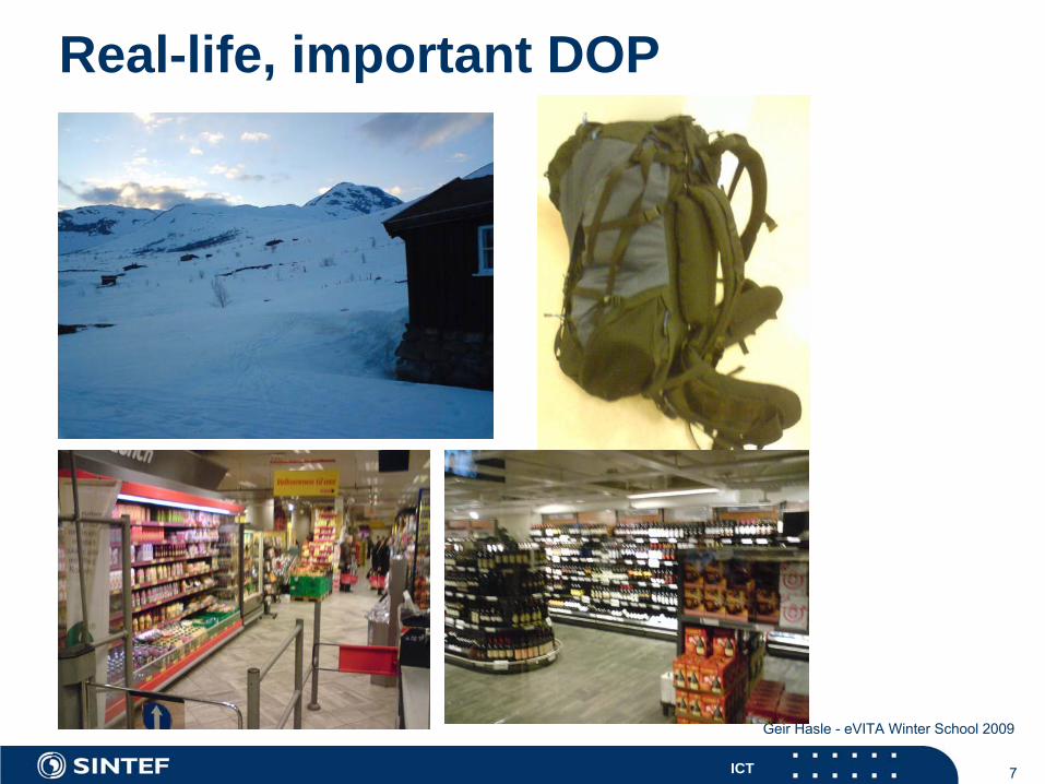
Real-life, important DOP
8ICT
Geir Hasle - eVITA Winter School 2009
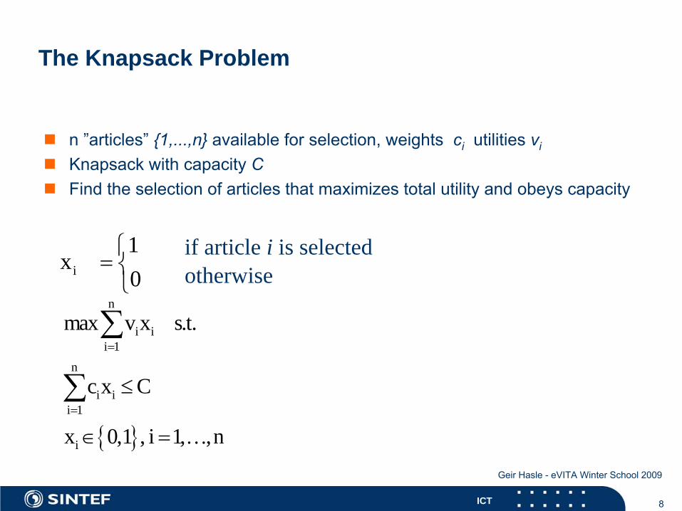
The Knapsack Problem
n ”articles” {1,...,n} available for selection, weights ci utilities vi
Knapsack with capacity CFind the selection of articles that maximizes total utility and obeys capacity
i
1x
0⎧
= ⎨⎩
if article i is selectedotherwise
{ }
n
i ii 1
n
i ii 1
i
max v x s.t.
c x C
x 0,1 , i 1, ,n
=
=
≤
∈ =
∑
∑…

9ICT
Geir Hasle - eVITA Winter School 2009
Example: – Selection of projects
You manage a large companyYour employees have suggested a large number of projects
resource requirementsutility
Fixed resource capacitySelect projects that will maximize utility
Strategic/tactical decisionDiscrete optimization problem
The Knapsack problem

10ICT
Geir Hasle - eVITA Winter School 2009
Example: - Transportation
You have a courier company and a carYou know your orders for tomorrow, pickup and delivery pointsYou know the travel time between all pointsYou want to finish as early as possible
Operational decisionDiscrete optimization problemThe Traveling Salesman Problem
11ICT
Geir Hasle - eVITA Winter School 2009
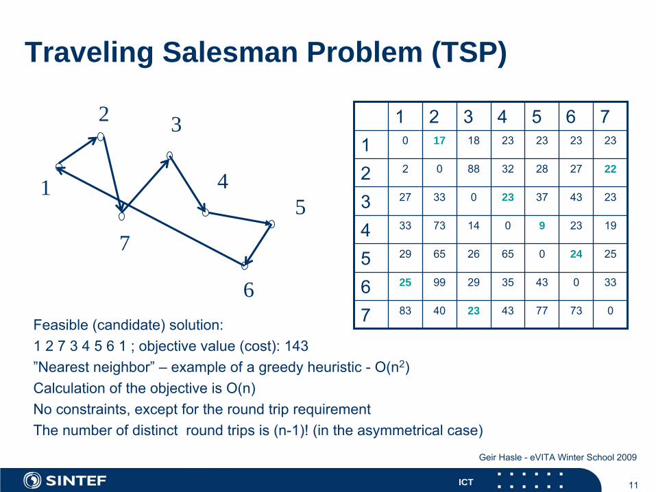
Traveling Salesman Problem (TSP)
Feasible
(candidate) solution: 1 2 7 3 4 5 6 1 ; objective
value
(cost): 143”Nearest
neighbor”
–
example
of
a greedy
heuristic
-
O(n2)Calculation
of
the
objective
is O(n)No constraints, except
for the
round
trip
requirementThe number
of
distinct
round
trips is (n-1)! (in the
asymmetrical
case)
1 2 3 4 5 6 71 0 17 18 23 23 23 23
2 2 0 88 32 28 27 22
3 27 33 0 23 37 43 23
4 33 73 14 0 9 23 19
5 29 65 26 65 0 24 25
6 25 99 29 35 43 0 33
7 83 40 23 43 77 73 0
1
2 3
45
6
7
12ICT
Geir Hasle - eVITA Winter School 2009
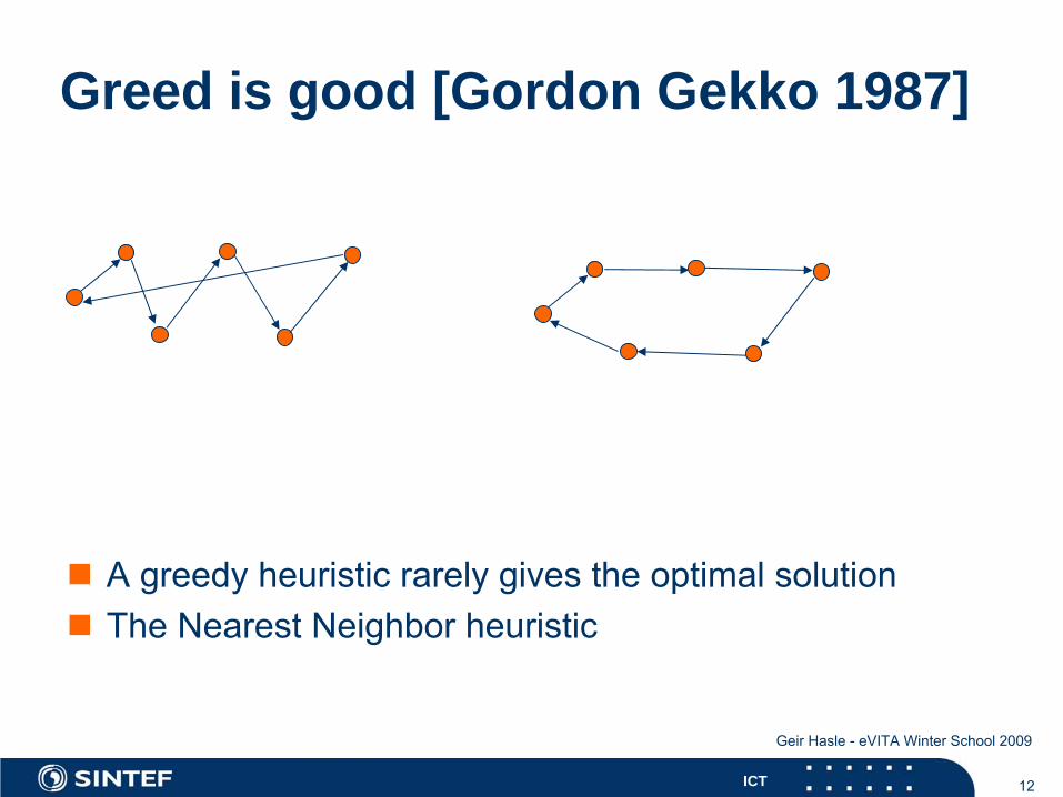
Greed is good [Gordon Gekko 1987]
A greedy heuristic rarely gives the optimal solutionThe Nearest Neighbor heuristic
13ICT
Geir Hasle - eVITA Winter School 2009
Problem (types) and problem instances
Example: TSPA type of concrete problems (instances)An instance is given by:
n: the number of citiesA: nxn-matrix of travel costs
14ICT
Geir Hasle - eVITA Winter School 2009
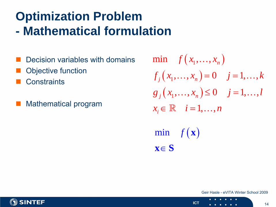
Optimization Problem - Mathematical formulation
Decision variables with domainsObjective functionConstraints
Mathematical program
( )( )( )
1
1
1
min , ,
, , 0 1, ,
, , 0 1, ,
1, ,
n
j n
j n
i
f x x
f x x j k
g x x j l
x i n
= =
≤ =
∈ =
…
… …
… ……
( )min f∈
xx S
15ICT
Geir Hasle - eVITA Winter School 2009
Linear Integer Programn
j jj 1
n
ij j ij 1
j
max c x s.t.
a x b i 1, ,m
x 0 j 1, , n
=
=
ζ =
≤ =
≥ =
∑
∑ …
…
{ }
n
j jj 1
n
ij j ij 1
0
j
i
max c x s.t.
a x b i 1, ,m
x 0 j 1,
x i I 1,
,
,
n
n
=
=
ζ =
=
∈
≤ =
≥
∈ ⊆
∑
∑ …
…
…
N
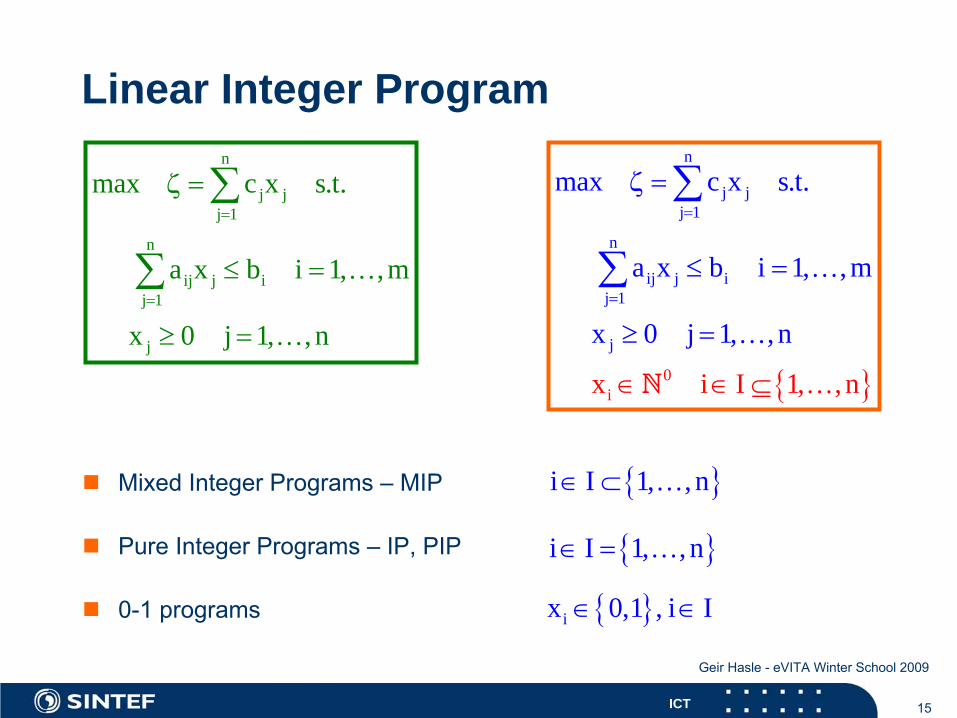
Mixed Integer Programs – MIP
Pure Integer Programs – IP, PIP
0-1 programs
{ }i I 1, , n∈ ⊂ …
{ }i I 1, , n∈ = …
{ }ix 0,1 , i I∈ ∈
16ICT
Geir Hasle - eVITA Winter School 2009
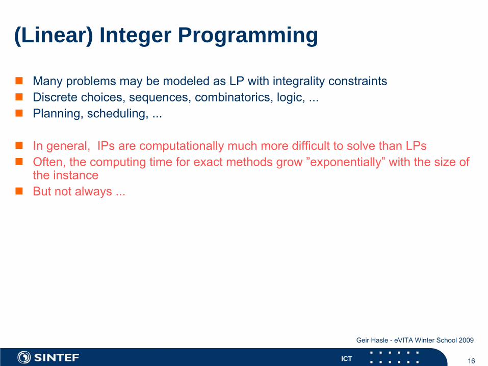
(Linear) Integer Programming
Many problems may be modeled as LP with integrality constraintsDiscrete choices, sequences, combinatorics, logic, ...Planning, scheduling, ...
In general, IPs are computationally much more difficult to solve than LPsOften, the computing time for exact methods grow ”exponentially” with the size ofthe instanceBut not always ...
17ICT
Geir Hasle - eVITA Winter School 2009
Definition – Discrete Optimization Problem
A Discrete
Optimization
Problem (DOP) iseither a minimization or maximization problemspecified by a set of problem instances
18ICT
Geir Hasle - eVITA Winter School 2009
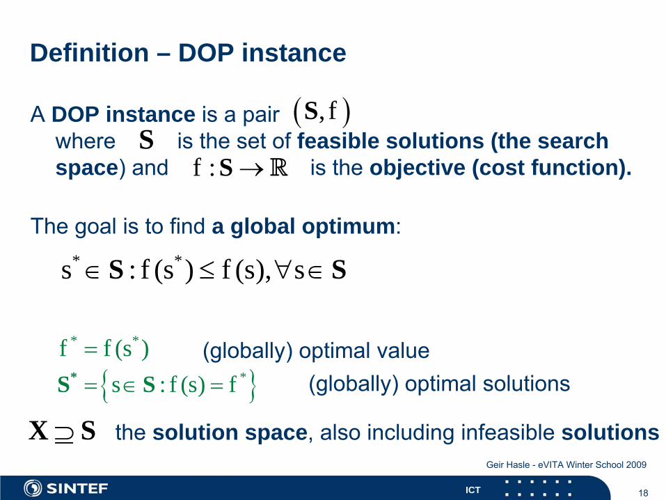
Definition – DOP instance
A DOP instance is a pair where
is the
set
of
feasible solutions (the search
space) and is the
objective (cost function).
The goal is to find
a global optimum:
f : →S R
( ), fS
* *s : f (s ) f (s), s∈ ≤ ∀ ∈S S
S
* *f f (s )= (globally) optimal value
{ }*s : f (s) f= ∈ =*S S (globally) optimal solutions
⊇X S the
solution space, also
including
infeasible
solutions
19ICT
Geir Hasle - eVITA Winter School 2009
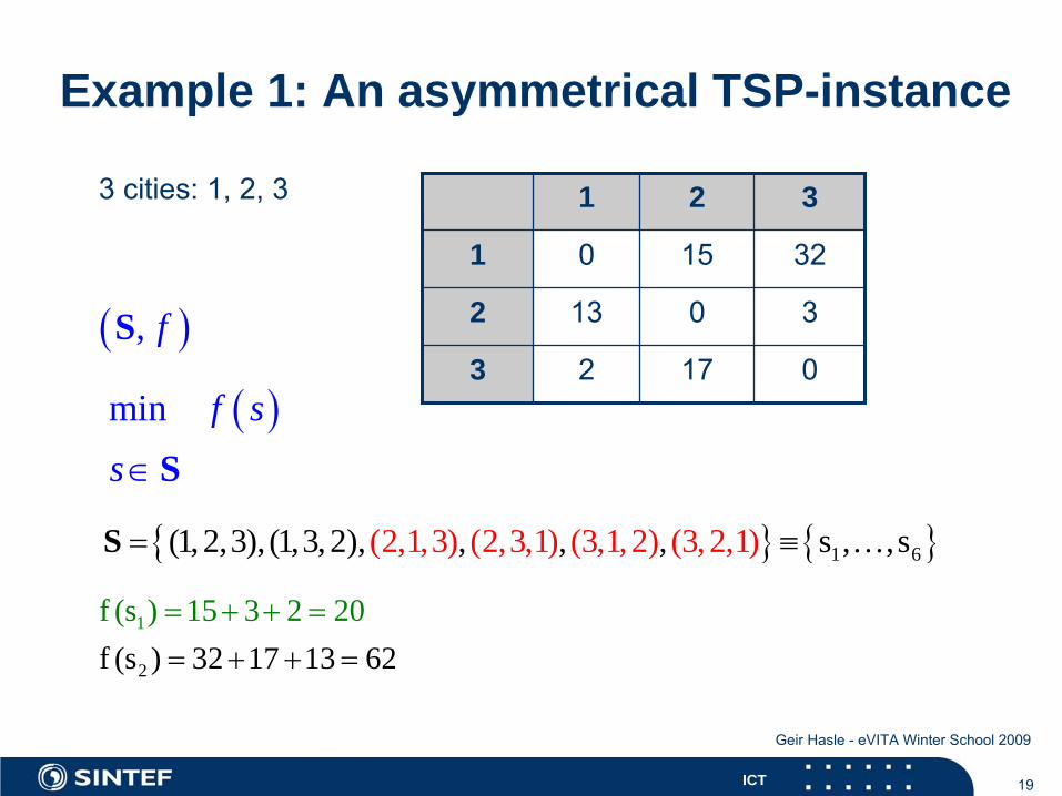
Example 1: An asymmetrical TSP-instance
3 cities: 1, 2, 3
{ } { }1 6(2,1,3) (2,3,1) (3,1,2(1,2,3) ) (3,2, (1,3, 2), , , , s1) ,s, ,= ≡S …
1 2 3
1 0 15 32
2 13 0 3
3 2 17 0
1
2f (f (
s ) 32 17 13s ) 15 20
62
23
= + += +
=+ =
( )min f ss∈S
( ), fS
20ICT
Geir Hasle - eVITA Winter School 2009
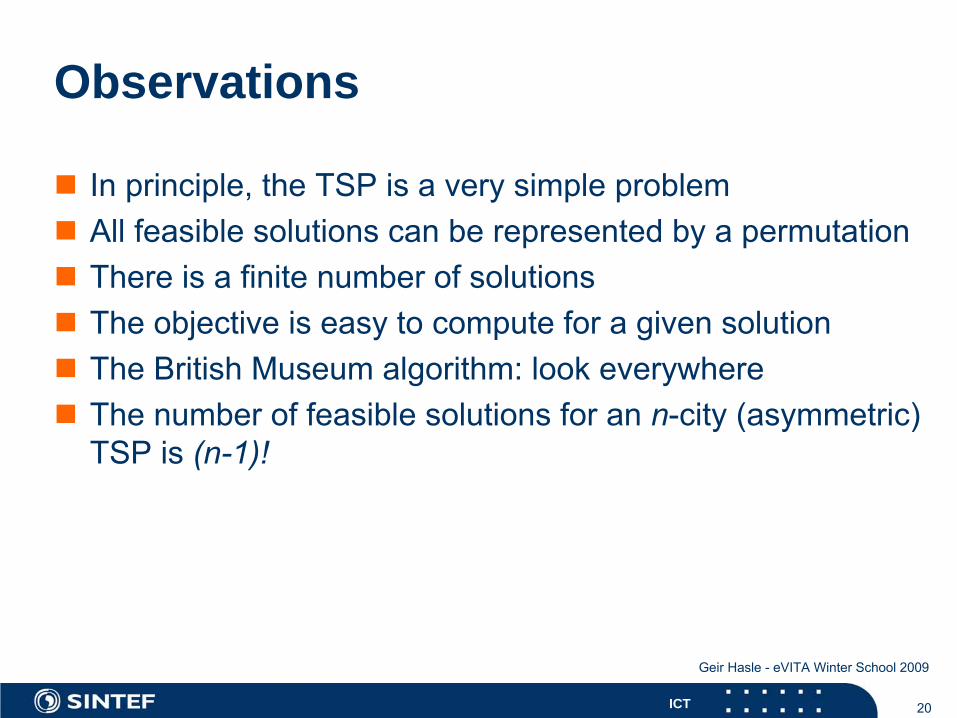
Observations
In principle, the TSP is a very simple problemAll feasible solutions can be represented by a permutationThere is a finite number of solutionsThe objective is easy to compute for a given solutionThe British Museum algorithm: look everywhereThe number of feasible solutions for an n-city (asymmetric) TSP is (n-1)!

21ICT
Geir Hasle - eVITA Winter School 2009
Combinatorial explosion
933262154439441526816992388856266700490715968264381621468592963895217599993229915608941463976156518286253697920827223758251185210916864000000000000000000000000100!
362880010! 106
243290200817664000020! 1019
30414093201713378043612608166064768844377641568966051200000000000050! 1065
10159
~ # atoms in our
galaxy# atoms in the
universe
~1080
# nanoseconds
since
Big Bang ~1026
22ICT
Geir Hasle - eVITA Winter School 2009
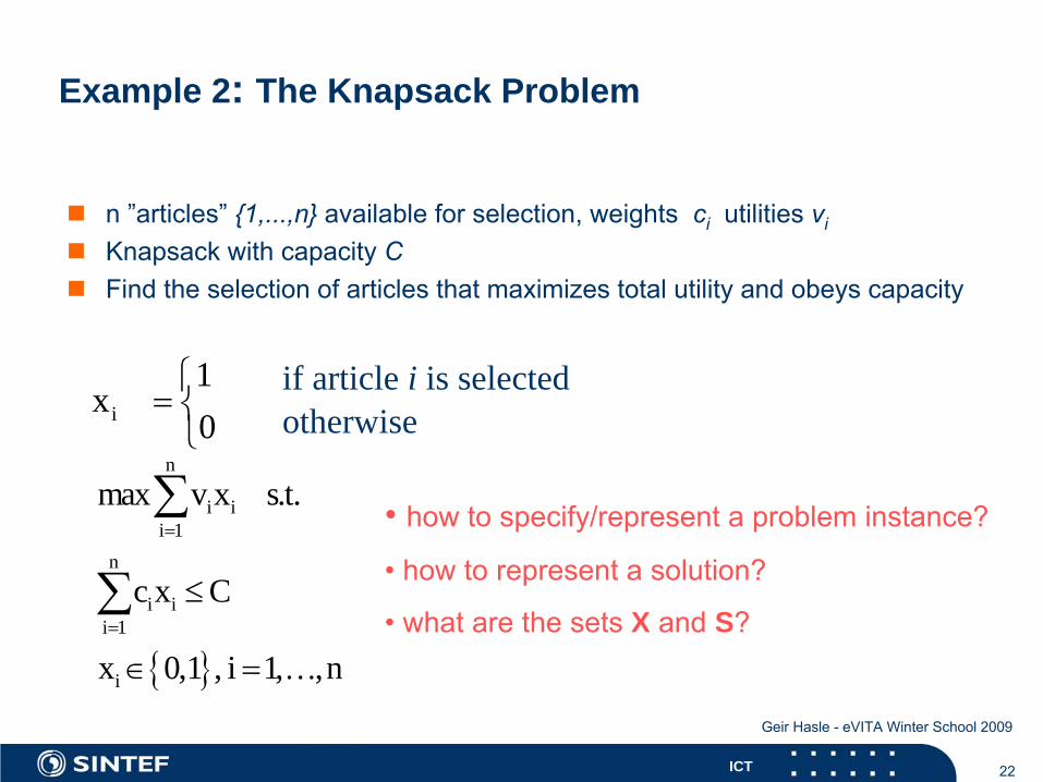
Example 2: The Knapsack Problem
n ”articles” {1,...,n} available for selection, weights ci utilities vi
Knapsack with capacity CFind the selection of articles that maximizes total utility and obeys capacity
i
1x
0⎧
= ⎨⎩
if article i is selectedotherwise
{ }
n
i ii 1
n
i ii 1
i
max v x s.t.
c x C
x 0,1 , i 1, ,n
=
=
≤
∈ =
∑
∑…
• how
to specify/represent
a problem instance?
• how
to represent
a solution?
• what
are
the
sets
X and S?
23ICT
Geir Hasle - eVITA Winter School 2009
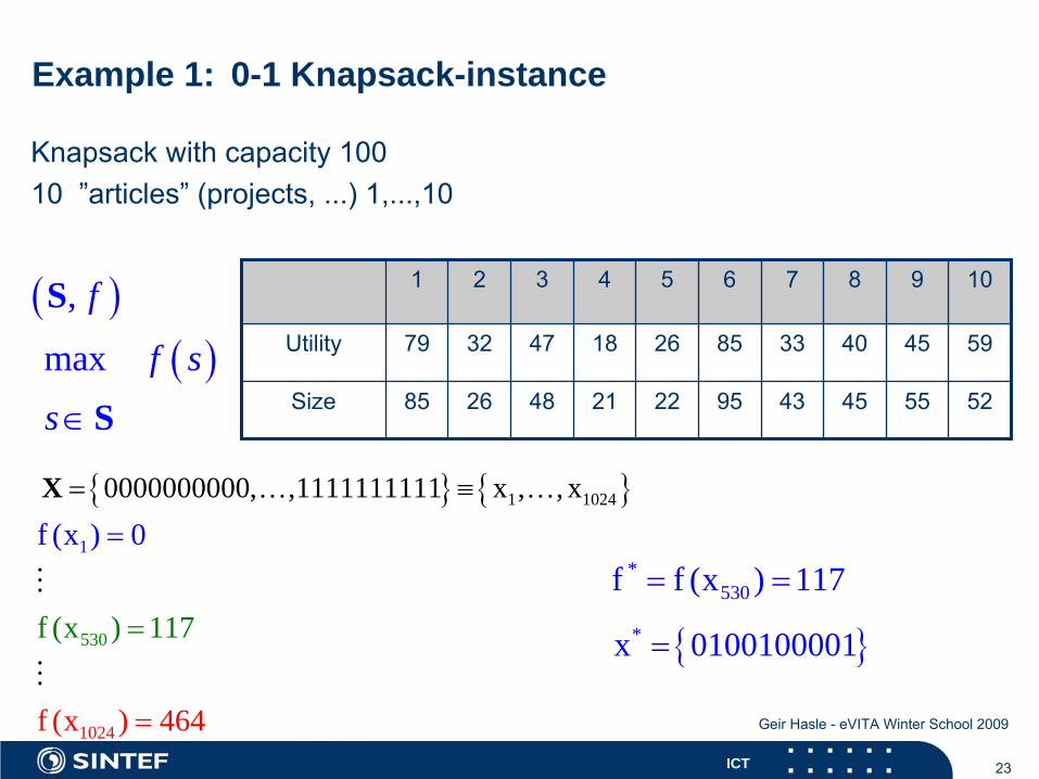
Example 1: 0-1 Knapsack-instance
Knapsack
with
capacity
10010 ”articles”
(projects, ...) 1,...,10
{ } { }1 10240000000000, ,1111111111 x , , x= ≡X … …
1
53
1
024
0f (x ) 1
f (x
f (x )
1
) 464
7
0
=
=
=
( )max f ss∈S
( ), fS 1 2 3 4 5 6 7 8 9 10
Utility 79 32 47 18 26 85 33 40 45 59
Size 85 26 48 21 22 95 43 45 55 52
*530f f (x ) 117= =
{ }*x 0100100001=
24ICT
Geir Hasle - eVITA Winter School 2009
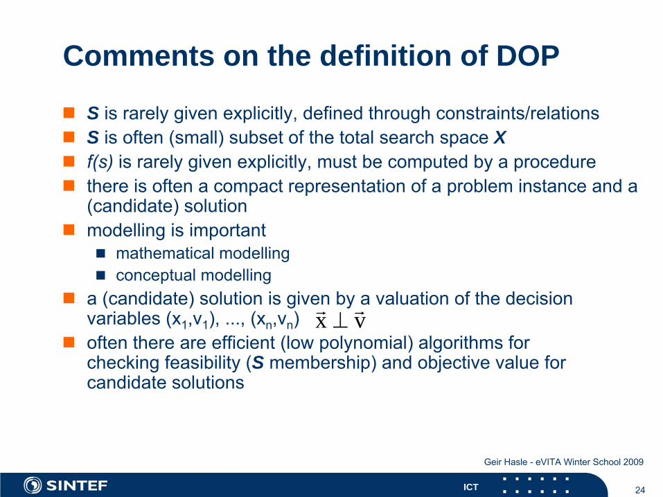
Comments on the definition of DOP
S is rarely given explicitly, defined through constraints/relationsS is often (small) subset of the total search space Xf(s) is rarely given explicitly, must be computed by a procedurethere is often a compact representation of a problem instance and a (candidate) solutionmodelling is important
mathematical modellingconceptual modelling
a (candidate) solution is given by a valuation of the decisionvariables (x1,v1), ..., (xn,vn)often there are efficient (low polynomial) algorithms forchecking feasibility (S membership) and objective value for candidate solutions
x v⊥
25ICT
Geir Hasle - eVITA Winter School 2009
DOP Applications
Decision problems with discrete alternativesSynthesis problems
planning, schedulingconfiguration, design
Limited resourcesOR, AILogistics, design, planlegging, roboticsGeometry, Image analysis, Finance ...
26ICT
Geir Hasle - eVITA Winter School 2009
Solution methods for DOP
Exact methods that guarantee to find an (all) optimal solution(s)
generate and test, explicit enumerationmathematical programming
Approximation methodswith quality guaranteesheuristics
Collaborative methods
27ICT
Geir Hasle - eVITA Winter School 2009
Computational Complexity Theory
Computing time (memory requirements) for problem types“the best” algorithmover all instancesas function of problem size
“Exponential” growth is cruel ...Parallel computing and general speed increase does not help muchProblem type is considered tractable only of there is a polynomial time algorithm for it
Worst case, pessimistic theoryOne problem instance is enough to deem a problem type as computationally intractable
28ICT
Geir Hasle - eVITA Winter School 2009
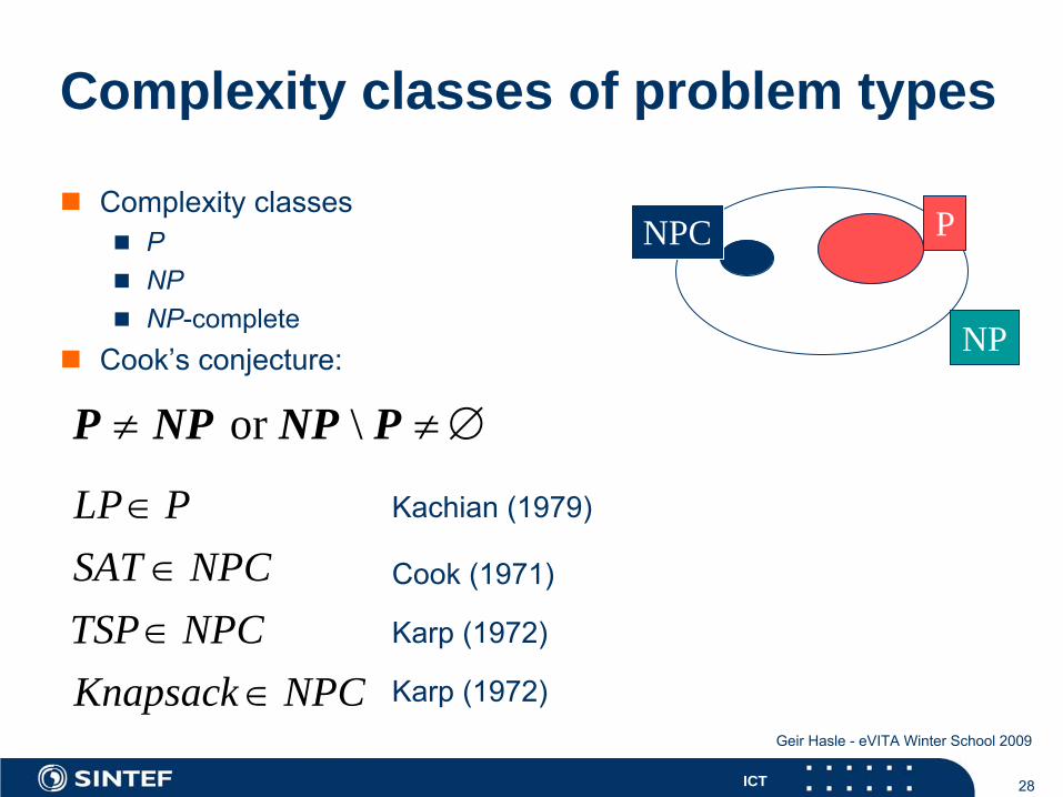
Complexity classes of problem types
Complexity classesPNPNP-complete
Cook’s conjecture:
or \≠ ≠ ∅P NP NP P
NPC P
NP
LP PSAT NPCTSP NPCKnapsack NPC
∈∈∈
∈
Kachian
(1979)
Cook (1971)
Karp (1972)
Karp (1972)
29ICT
Geir Hasle - eVITA Winter School 2009
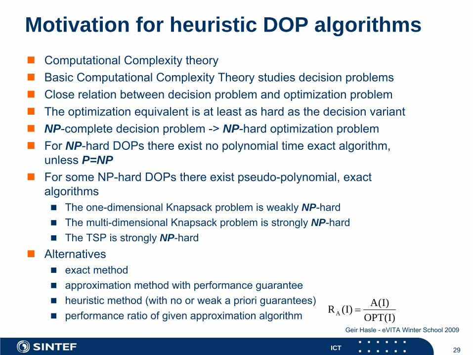
Motivation for heuristic DOP algorithmsComputational Complexity theoryBasic Computational Complexity Theory studies decision problemsClose relation between decision problem and optimization problemThe optimization equivalent is at least as hard as the decision variantNP-complete decision problem -> NP-hard optimization problemFor NP-hard DOPs there exist no polynomial time exact algorithm, unless P=NPFor some NP-hard DOPs there exist pseudo-polynomial, exact algorithms
The one-dimensional Knapsack problem is weakly NP-hardThe multi-dimensional Knapsack problem is strongly NP-hardThe TSP is strongly NP-hard
Alternativesexact methodapproximation method with performance guaranteeheuristic method (with no or weak a priori guarantees)performance ratio of given approximation algorithm A
A(I)R (I)OPT(I)
=
30ICT
Geir Hasle - eVITA Winter School 2009
Some messages (1)
Not all DOPs are NP-hard, e.g., the Assignment ProblemEven NP-hard problems may be effectively solved
small instancesspecial structureweakly NP-hard
Even large instances of strongly NP-hard problems may be effectivelysolved to optimality
TSPs with a few hundred cities in a few seconds
31ICT
Geir Hasle - eVITA Winter School 2009
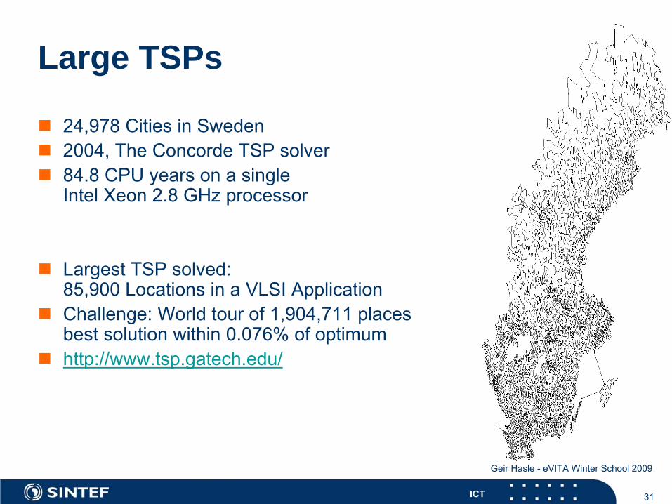
Large TSPs
24,978 Cities in Sweden2004, The Concorde TSP solver84.8 CPU years on a single Intel Xeon 2.8 GHz processor
Largest TSP solved:85,900 Locations in a VLSI ApplicationChallenge: World tour of 1,904,711 placesbest solution within 0.076% of optimumhttp://www.tsp.gatech.edu/

32ICT
Geir Hasle - eVITA Winter School 2009
VRP with Capacity Constraints (CVRP) Graph G=(N,A)
N={0,…,n+1} Nodes0 Depot, i≠0 Customers A={(i,j): i,j∈N} Arcscij >0 Transportation Costs
Demand di for each Customer iV set of identical Vehicles each with Capacity qGoal
Design a set of Routes that start and finish at the Depot - with minimal Cost.Each Customer to be visited only once (no order splitting)Total Demand for all Customers not to exceed CapacityCost: weighted sum of Driving Cost and # Routes
DVRP – distance/time constraint on each routeVRPTW – VRP with time windowsPickup and Delivery
Backhaul – VRPB(TW)Pickup and delivery VRPPD(TW)PDP
I aI b
I c
I d
I eI f
I g
I hIi
Ij
2
3Ik
IlImInIo
Ip 41
IlIm
IkInIo
IpI e
I d
I c
I aI bI g
I hIi
IjI f1
2
3
4
33ICT
Geir Hasle - eVITA Winter School 2009
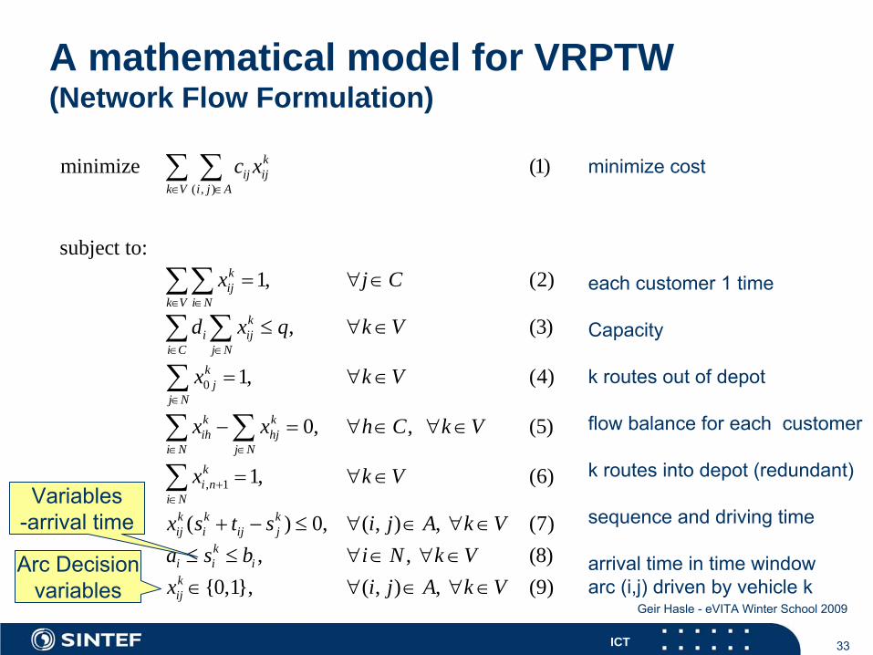
A mathematical model for VRPTW (Network Flow Formulation)
( , )
0
, 1
minimize (1)
subject to:1, (2)
, (3)
1, (4)
0, , (5)
1, (6)
( ) 0, ( , ) , (7)
∈ ∈
∈ ∈
∈ ∈
∈
∈ ∈
+∈
= ∀ ∈
≤ ∀ ∈
= ∀ ∈
− = ∀ ∈ ∀ ∈
= ∀ ∈
+ − ≤ ∀ ∈ ∀ ∈
∑ ∑
∑∑∑ ∑
∑
∑ ∑
∑
kij ij
k V i j A
kij
k V i Nk
i iji C j N
kj
j Nk kih hj
i N j Nki n
i Nk k kij i ij j
i
c x
x j C
d x q k V
x k V
x x h C k V
x k V
x s t s i j A k Va , , (8)
{0,1}, ( , ) , (9)≤ ≤ ∀ ∈ ∀ ∈∈ ∀ ∈ ∀ ∈
ki i
kij
s b i N k Vx i j A k V
minimize
cost
each
customer
1 time
Capacity
k routes
out
of
depot
flow
balance
for each
customer
k routes
into
depot (redundant)
sequence
and driving time
arrival
time in time windowarc
(i,j) driven by vehicle
k Arc Decision
variables
Variables-arrival time
34ICT
Geir Hasle - eVITA Winter School 2009
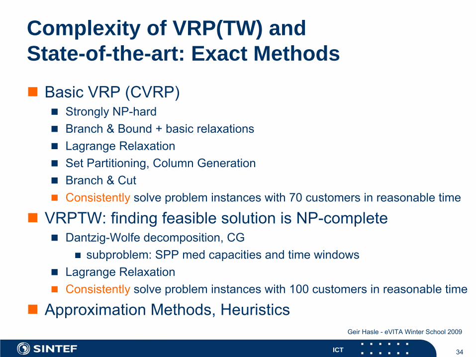
Complexity of VRP(TW) and State-of-the-art: Exact Methods
Basic VRP (CVRP)Strongly NP-hardBranch & Bound + basic relaxationsLagrange RelaxationSet Partitioning, Column GenerationBranch & CutConsistently solve problem instances with 70 customers in reasonable time
VRPTW: finding feasible solution is NP-completeDantzig-Wolfe decomposition, CG
subproblem: SPP med capacities and time windowsLagrange RelaxationConsistently solve problem instances with 100 customers in reasonable time
Approximation Methods, Heuristics
35ICT
Geir Hasle - eVITA Winter School 2009
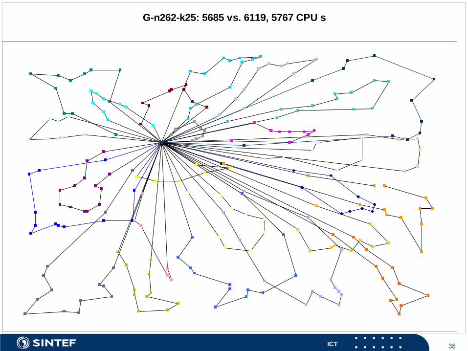
G-n262-k25: 5685 vs. 6119, 5767 CPU s
36ICT
Geir Hasle - eVITA Winter School 2009
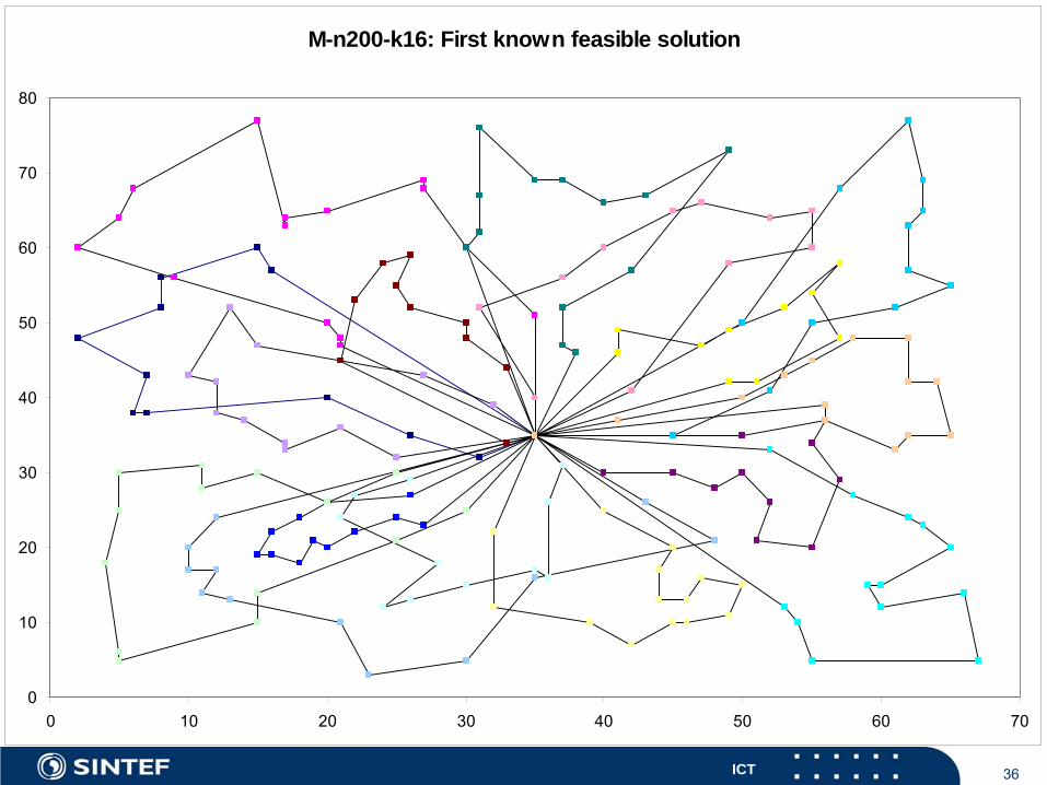
M-n200-k16: First known feasible solution
0
10
20
30
40
50
60
70
80
0 10 20 30 40 50 60 70

37ICT
Geir Hasle - eVITA Winter School 2009
Some messages (2)
DOPs should be analyzedTry exact methodsCollaboration between exact and heuristic methods
a good, heuristic solution may jump-start and speed up an exact methodexact methods may give high quality boundstrue collaboration, asynchronous parallel algorithms
38ICT
Geir Hasle - eVITA Winter School 2009
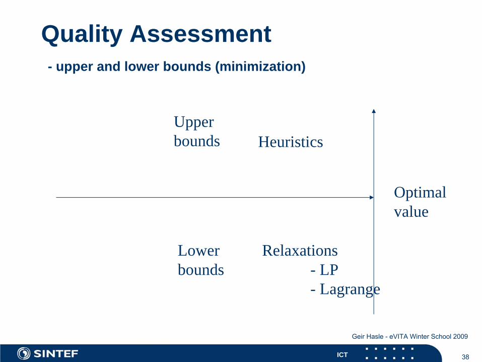
Quality Assessment - upper and lower bounds (minimization)
Optimalvalue
Upperbounds
Lowerbounds
Heuristics
Relaxations- LP- Lagrange
39ICT
Geir Hasle - eVITA Winter School 2009
Further motivation - heuristicsIn the real world
response requirementsinstance size and response requirements may rule out exact methodsoptimization is just one aspectmodelling challenges, what is the objective?humans are satisficers, not optimizers [Herb Simon]generic solver, all kinds of instances, robustness
Heuristic methods are generally robust, few drastic assumptions
Exact methods should not be disqualified a prioriCultures
mathematicians vs. engineers/pragmatistsOR vs. AI animosityreconciliation
40ICT
Geir Hasle - eVITA Winter School 2009
Exact methods for DOPDOPs typically have a finite # solutionsExact methods guarantee to find an optimal solutionResponse time?
Good for solving limited size instancesMay be good for the instances in questionSome (weakly) NP-hard problems are effectively solved, given assumptions on input data Basis for approximation methodsSubproblems, reduced or relaxed problems

41ICT
Geir Hasle - eVITA Winter School 2009
Heuristics - definitionsWikipedia: “Heuristics stand for strategies using readily accessible, thoughloosely applicable, information to control problem-solving in human beings and machines”.Greek: (h)eureka – “I have found it”, Archimedes 3rd century BCPsychology: Heuristics are simple, efficient rules, hard-coded by evolutionary processes or learned, which have been proposed to explain how people make decisions, come to judgments, and solve problems, typically when facing complex problems or incomplete information. Work well under most circumstances, but in certain cases lead to systematic cognitive biases. Mathematics: “How to solve it” [G. Polya 1957]. Guide to solution of mathematical problems.AI: Techniques that improve the efficiency of a search process often by sacrificing completenessComputing science: Algorithms that ignore whether the solution to the problem can be proven to be correct, but which usually produces a good solution or solves a simpler problem that contains, or intersects with, the solution of the more complex problem. Heuristics are typically used when there is no known way to find an optimal solution, or when it is desirable to give up finding the optimal solution for an improvement in run time.
42ICT
Geir Hasle - eVITA Winter School 2009
Heuristics in Discrete Optimization
Sacrificing the guarantee of finding the optimal solutionStrong guarantees regarding solution quality vs. response time typically cannot be given
General heuristicsstrategies for traversing the Branch & Bound tree in MIP
Greedy heuristicsSpecial heuristics, exploiting problem structureBasic method: Local SearchBetter methods: Metaheuristics
43ICT
Geir Hasle - eVITA Winter School 2009
How to find a DOP solution?Exact methods
Earlier solutionTrivial solutionRandom solutionConstructive method
gradual build-up of solutions from scratchgreedy heuristic
Solve simpler problemremove or change constraintsmodify objective
Given a solution, modify it
44ICT
Geir Hasle - eVITA Winter School 2009
Local Search and Meta-Heuristics
Operate on a ”natural” representation of solutionsThe combinatorial objectSearch in the space of feasible solutions / all solutions(search space, solution space)
Single solution: Trajectory based methodsMultiple solutions: Population based methods
45ICT
Geir Hasle - eVITA Winter School 2009
Local search for DOP
Dates back to late 1950ies, TSP workRenaissance in the past 20 yearsHeuristic methodBased on small modifications of given solutionIngredients:
Initial solutionOperator(s), Neighborhood(s)Search strategyStop criterion
Iterative methodAnytime method
46ICT
Geir Hasle - eVITA Winter School 2009
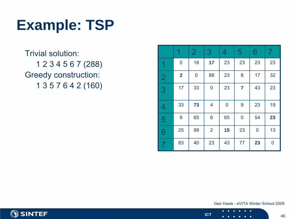
Example: TSP
Trivial solution:1 2 3 4 5 6 7 (288)
Greedy
construction:1 3 5 7 6 4 2 (160)
1 2 3 4 5 6 71 0 18 17 23 23 23 23
2 2 0 88 23 8 17 32
3 17 33 0 23 7 43 23
4 33 73 4 0 9 23 19
5 9 65 6 65 0 54 23
6 25 99 2 15 23 0 13
7 83 40 23 43 77 23 0
47ICT
Geir Hasle - eVITA Winter School 2009
Example: 0-1 Knapsack
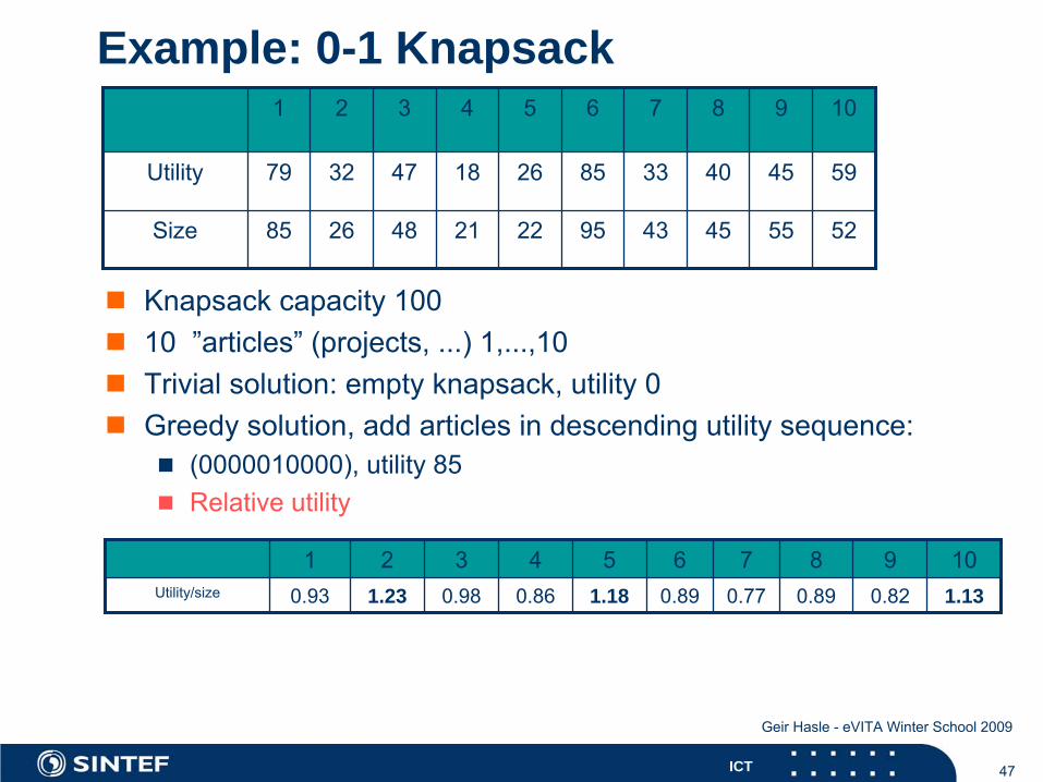
Knapsack capacity 10010 ”articles” (projects, ...) 1,...,10Trivial solution: empty knapsack, utility 0Greedy solution, add articles in descending utility sequence:
(0000010000), utility 85Relative utility
1 2 3 4 5 6 7 8 9 10
Utility 79 32 47 18 26 85 33 40 45 59
Size 85 26 48 21 22 95 43 45 55 52
1 2 3 4 5 6 7 8 9 10Utility/size 0.93 1.23 0.98 0.86 1.18 0.89 0.77 0.89 0.82 1.13
48ICT
Geir Hasle - eVITA Winter School 2009
Given a solution, how to find a better one?
Modification of given solution gives ”neighbor”A certain type of operation gives a set of neighbors: a neighborhoodEvaluation
objectivefeasibility
49ICT
Geir Hasle - eVITA Winter School 2009
Example: TSP
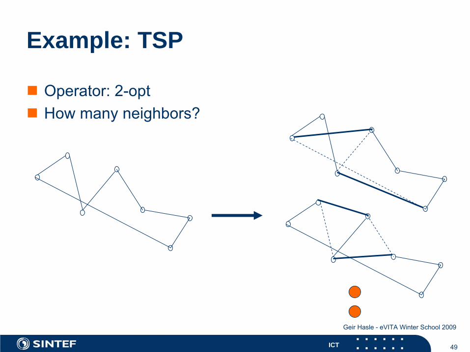
Operator: 2-optHow many neighbors?
50ICT
Geir Hasle - eVITA Winter School 2009
Example: Knapsack
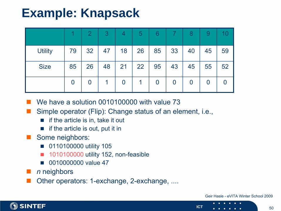
We have a solution 0010100000 with value 73Simple operator (Flip): Change status of an element, i.e.,
if the article is in, take it outif the article is out, put it in
Some neighbors:0110100000 utility 1051010100000 utility 152, non-feasible0010000000 value 47
n neighborsOther operators: 1-exchange, 2-exchange, ....
1 2 3 4 5 6 7 8 9 10
Utility 79 32 47 18 26 85 33 40 45 59
Size 85 26 48 21 22 95 43 45 55 52
0 0 1 0 1 0 0 0 0 0
51ICT
Geir Hasle - eVITA Winter School 2009
Definition: Neighborhood function
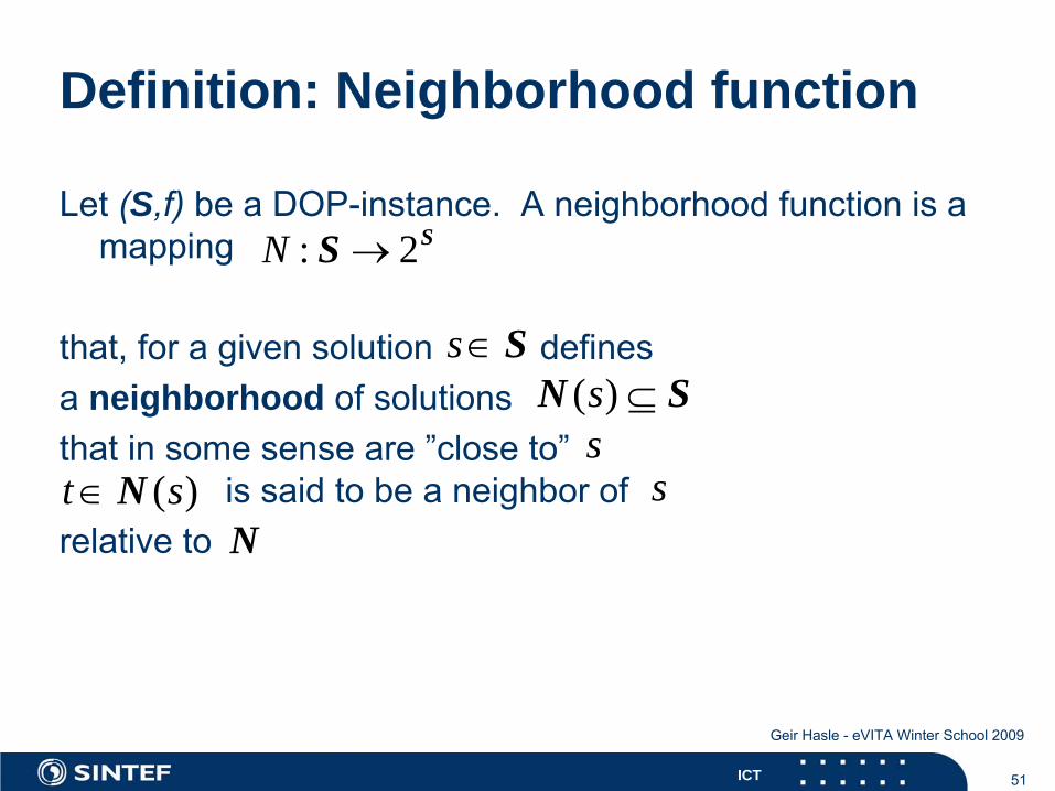
Let (S,f)
be a DOP-instance. A neighborhood
function
is a mapping
that, for a given solution defines
a neighborhood of
solutionsthat
in some
sense
are
”close
to”
is said
to be a neighbor
ofrelative to
: 2→N SS
∈s S( ) ⊆sN Ss
( )∈t sN sN
52ICT
Geir Hasle - eVITA Winter School 2009
Neighborhood operator
Neighborhood functions are often defined through certain genericoperations on a solution - operatorNormally rather simple operations on key structures in thecombinatorial object
removal of an elementaddition of an elementexchange of two or more elements
Multiple neighborhood functions - qualification by operator ( ),N sσ σ∈Σ
53ICT
Geir Hasle - eVITA Winter School 2009
Local Search (Neighborhood Search)
Starting point: initial solutionIterative search in neighborhoods for better solutionSequence/path of solutions
Path is determined byInitial solutionNeighborhood functionAcceptance strategyStop criterion
What happens when the neighborhood contains no better solution?Local optimum
1 ( ), 0,k ks N s k+ σ∈ = …
0s
54ICT
Geir Hasle - eVITA Winter School 2009
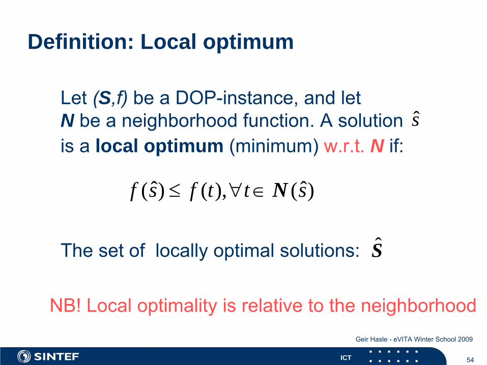
Definition: Local optimum
Let (S,f)
be a DOP-instance, and letN be a neighborhood
function. A solution
is a local optimum (minimum) w.r.t. N if:s
ˆ ˆ( ) ( ), ( )≤ ∀ ∈f s f t t sN
The set
of
locally
optimal solutions: S
NB! Local
optimality
is relative to the
neighborhood
55ICT
Geir Hasle - eVITA Winter School 2009
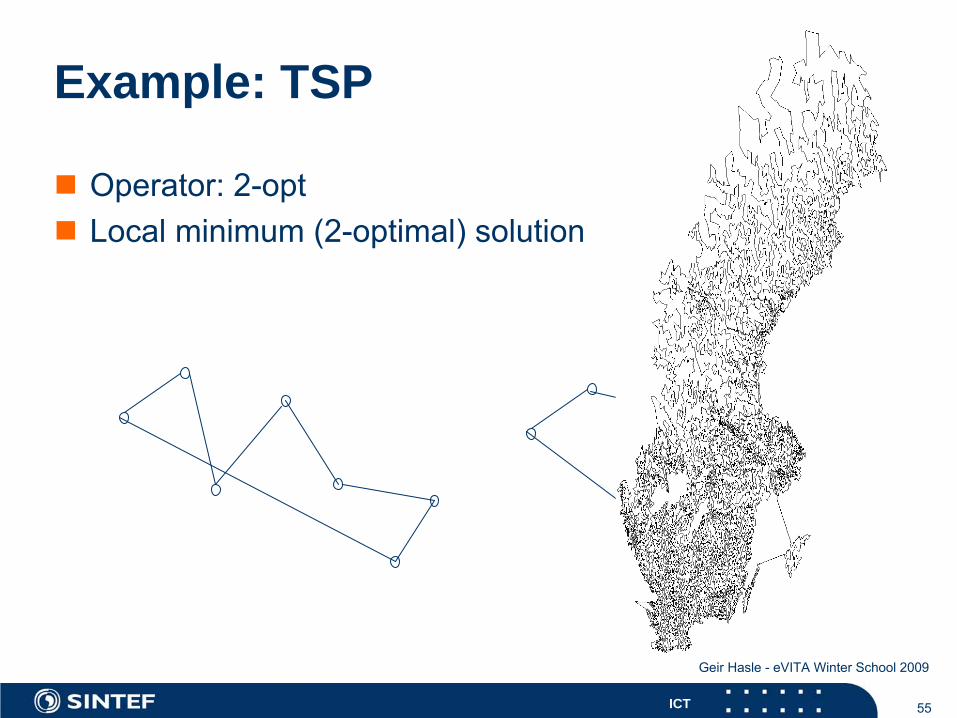
Example: TSP
Operator: 2-optLocal minimum (2-optimal) solution
56ICT
Geir Hasle - eVITA Winter School 2009
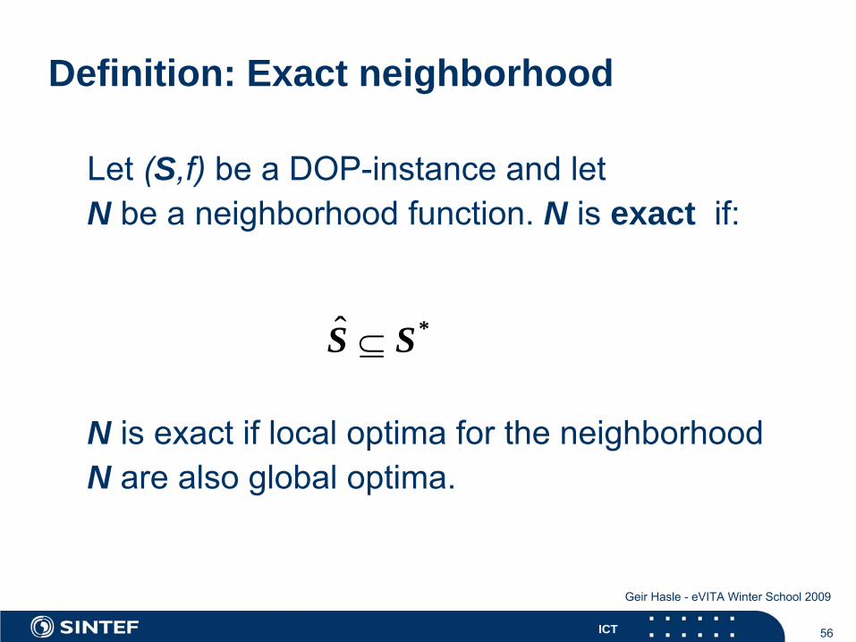
Definition: Exact neighborhood
Let (S,f)
be a DOP-instance
and letN be a neighborhood
function. N is exact if:
ˆ ⊆S S*
N is exact
if
local
optima for the
neighborhoodN are
also
global optima.
57ICT
Geir Hasle - eVITA Winter School 2009
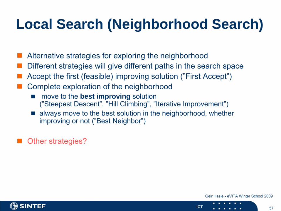
Local Search (Neighborhood Search)
Alternative strategies for exploring the neighborhoodDifferent strategies will give different paths in the search spaceAccept the first (feasible) improving solution (”First Accept”)Complete exploration of the neighborhood
move to the best improving solution(”Steepest Descent”, ”Hill Climbing”, ”Iterative Improvement”)always move to the best solution in the neighborhood, whetherimproving or not (”Best Neighbor”)
Other strategies?
58ICT
Geir Hasle - eVITA Winter School 2009
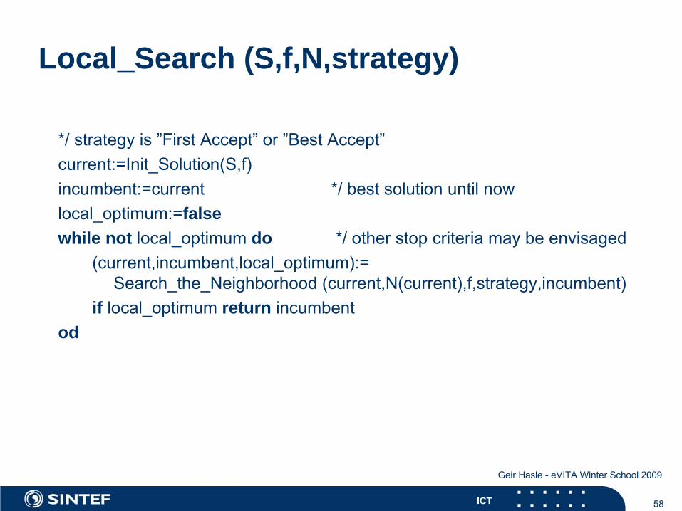
Local_Search (S,f,N,strategy)
*/ strategy
is ”First Accept”
or ”Best Accept”current:=Init_Solution(S,f)incumbent:=current
*/ best solution
until
now
local_optimum:=falsewhile not local_optimum
do */ other
stop
criteria
may
be envisaged
(current,incumbent,local_optimum):= Search_the_Neighborhood
(current,N(current),f,strategy,incumbent)
if local_optimum
return incumbentod
59ICT
Geir Hasle - eVITA Winter School 2009
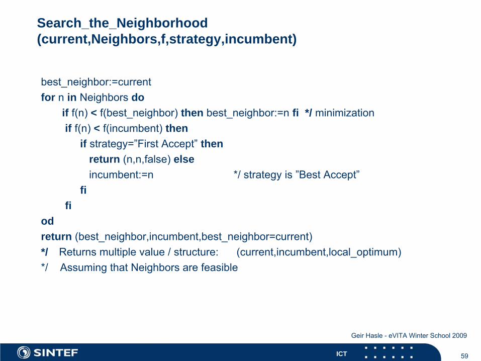
Search_the_Neighborhood (current,Neighbors,f,strategy,incumbent)
best_neighbor:=currentfor n
in Neighbors
doif f(n)
< f(best_neighbor)
then best_neighbor:=n
fi */ minimizationif f(n) < f(incumbent) then
if strategy=”First
Accept”
thenreturn (n,n,false) elseincumbent:=n
*/ strategy
is ”Best Accept”fi
fiodreturn (best_neighbor,incumbent,best_neighbor=current)*/ Returns
multiple value
/ structure: (current,incumbent,local_optimum)*/ Assuming
that
Neighbors
are
feasible
60ICT
Geir Hasle - eVITA Winter School 2009
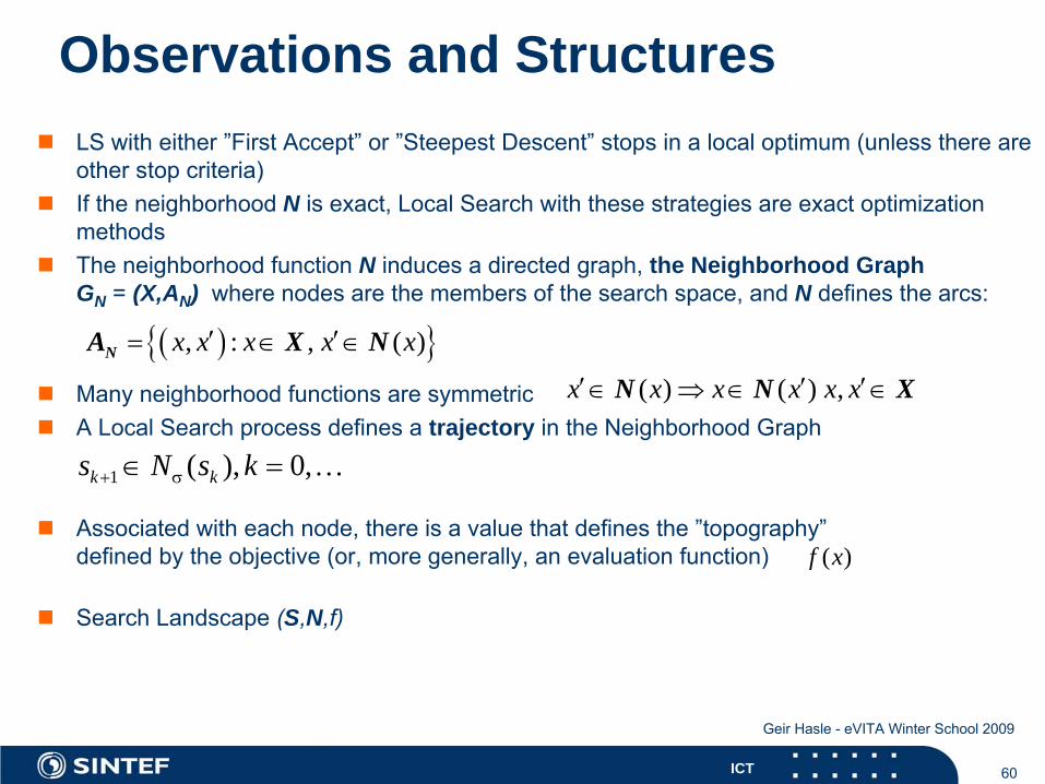
Observations and StructuresLS with either ”First Accept” or ”Steepest Descent” stops in a local optimum (unless there areother stop criteria)If the neighborhood N is exact, Local Search with these strategies are exact optimizationmethodsThe neighborhood function N induces a directed graph, the Neighborhood Graph GN = (X,AN) where nodes are the members of the search space, and N defines the arcs:
Many neighborhood functions are symmetricA Local Search process defines a trajectory in the Neighborhood Graph
Associated with each node, there is a value that defines the ”topography”defined by the objective (or, more generally, an evaluation function)
Search Landscape (S,N,f)
( ){ }, : , ( )′ ′= ∈ ∈x x x x xNA X N
( ) ( ) ,′ ′ ′∈ ⇒ ∈ ∈x x x x x xN N X
1 ( ), 0,k ks N s k+ σ∈ = …
( )f x
61ICT
Geir Hasle - eVITA Winter School 2009
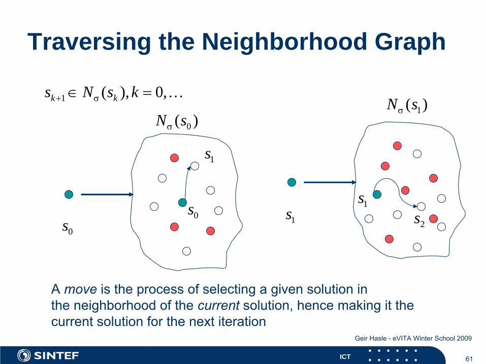
Traversing the Neighborhood Graph
1 ( ), 0,k ks N s k+ σ∈ = …
0s 1s
0( )N sσ
1s
0s
1( )N sσ
2s1s
A move
is
the
process
of
selecting
a given solution
in the
neighborhood
of
the
current
solution, hence
making it the
current
solution
for the
next
iteration
62ICT
Geir Hasle - eVITA Winter School 2009
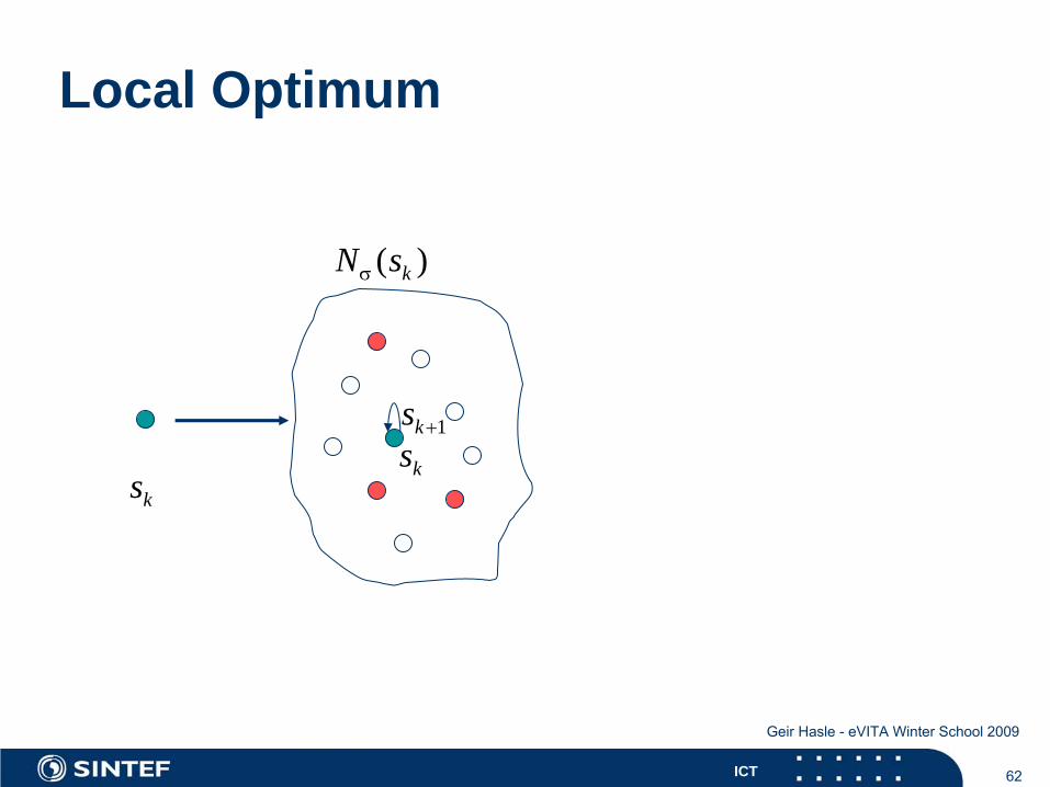
Local Optimum
ks
( )kN sσ
1ks +
ks

63ICT
Geir Hasle - eVITA Winter School 2009
Search Landscapes - Local and global optima
Objective value
Solution space
64ICT
Geir Hasle - eVITA Winter School 2009
Simplex algorithm for LP as Local Search
Simplex Phase I gives initial, feasible solution (if it exists)Phase II gives iterative improvement towards optimal solution (if it exists)The neighborhood is defined by the polyhedronThe strategy is ”Iterative Improvement”The concrete moves are determined by pivoting rulesThe neighborhood is exact, i.e., Simplex is an exact optimization algorithm(for certain pivoting rules)
65ICT
Geir Hasle - eVITA Winter School 2009
Local SearchMain challenges
feasible region only, or the whole solution space? design good neighborhoodssize, scalability, search landscapeinitial solutionstrategyefficient evaluation of the neighborhoods
incremental evaluation of constraintsincremental evaluation of the objective (evaluation function)
stop criteriaperformance guarantees
The performance is typically much better than greedy heuristics
66ICT
Geir Hasle - eVITA Winter School 2009
Design of neighborhood operators
Based on natural attributesNeighborhood size, scalabilityDiameter: maximum # moves to get from one solution to anotherConnectivity
Search complexity depends on Search Landscape
Distance metricsHamming distance, Edit distance
67ICT
Geir Hasle - eVITA Winter School 2009
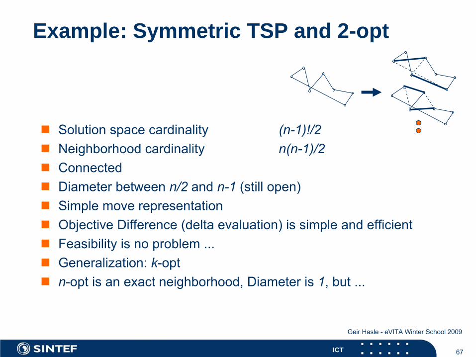
Example: Symmetric TSP and 2-opt
Solution space cardinality (n-1)!/2Neighborhood cardinality n(n-1)/2ConnectedDiameter between n/2 and n-1 (still open)Simple move representationObjective Difference (delta evaluation) is simple and efficientFeasibility is no problem ...Generalization: k-optn-opt is an exact neighborhood, Diameter is 1, but ...
68ICT
Geir Hasle - eVITA Winter School 2009
Diameter of 0-1 Knapsack problem with the ”Flip” neighborhood
One is never more than n moves away from the optimal solutionbut the landscape you have to move through may be very bumpy ...
=X n2
69ICT
Geir Hasle - eVITA Winter School 2009
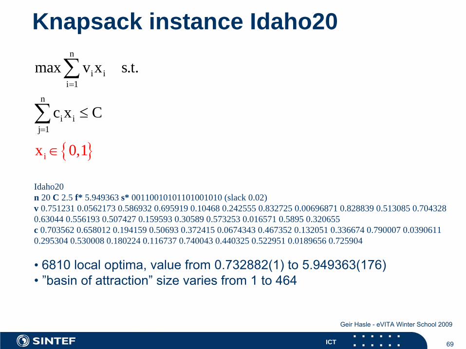
Knapsack instance Idaho20
{ }
n
i ii 1
n
i ij
i
1
max v x s.t.
c
x
x C
0,1
=
=
∈
≤
∑
∑
Idaho20n 20 C 2.5 f* 5.949363 s* 00110010101101001010 (slack 0.02)v 0.751231 0.0562173 0.586932 0.695919 0.10468 0.242555 0.832725 0.00696871 0.828839 0.513085 0.704328 0.63044 0.556193 0.507427 0.159593 0.30589 0.573253 0.016571 0.5895 0.320655c 0.703562 0.658012 0.194159 0.50693 0.372415 0.0674343 0.467352 0.132051 0.336674 0.790007 0.0390611 0.295304 0.530008 0.180224 0.116737 0.740043 0.440325 0.522951 0.0189656 0.725904
• 6810 local
optima, value
from 0.732882(1) to 5.949363(176) • ”basin
of
attraction”
size
varies
from 1 to 464

70ICT
Geir Hasle - eVITA Winter School 2009
Search landscape for Idaho20LO Value
0
1
2
3
4
5
6
7
1 272 543 814 1085 1356 1627 1898 2169 2440 2711 2982 3253 3524 3795 4066 4337 4608 4879 5150 5421 5692 5963 6234 6505 6776
LO Value
Frequency
050
100150200250300350400450500
1 278 555 832 1109 1386 1663 1940 2217 2494 2771 3048 3325 3602 3879 4156 4433 4710 4987 5264 5541 5818 6095 6372 6649
Frequency
71ICT
Geir Hasle - eVITA Winter School 2009
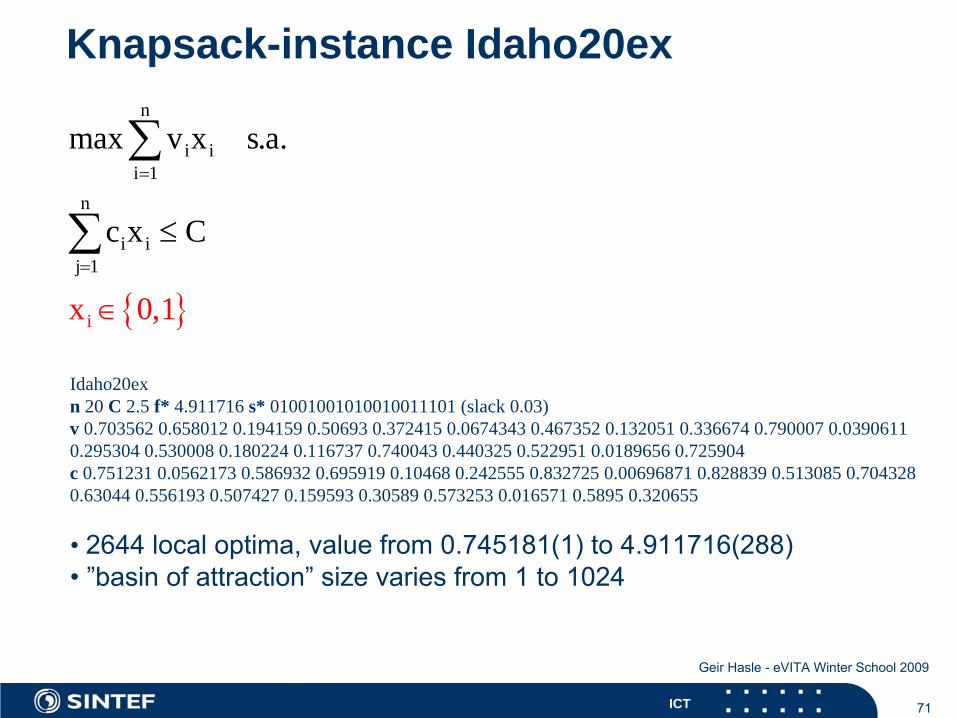
Knapsack-instance Idaho20ex
{ }
n
i ii 1
n
i ij
i
1
max v x s.a.
c
x
x C
0,1
=
=
∈
≤
∑
∑
Idaho20exn 20 C 2.5 f* 4.911716 s* 01001001010010011101 (slack 0.03)v 0.703562 0.658012 0.194159 0.50693 0.372415 0.0674343 0.467352 0.132051 0.336674 0.790007 0.0390611 0.295304 0.530008 0.180224 0.116737 0.740043 0.440325 0.522951 0.0189656 0.725904c 0.751231 0.0562173 0.586932 0.695919 0.10468 0.242555 0.832725 0.00696871 0.828839 0.513085 0.704328 0.63044 0.556193 0.507427 0.159593 0.30589 0.573253 0.016571 0.5895 0.320655
• 2644 local
optima, value
from 0.745181(1) to 4.911716(288) • ”basin
of
attraction”
size
varies
from 1 to 1024
72ICT
Geir Hasle - eVITA Winter School 2009
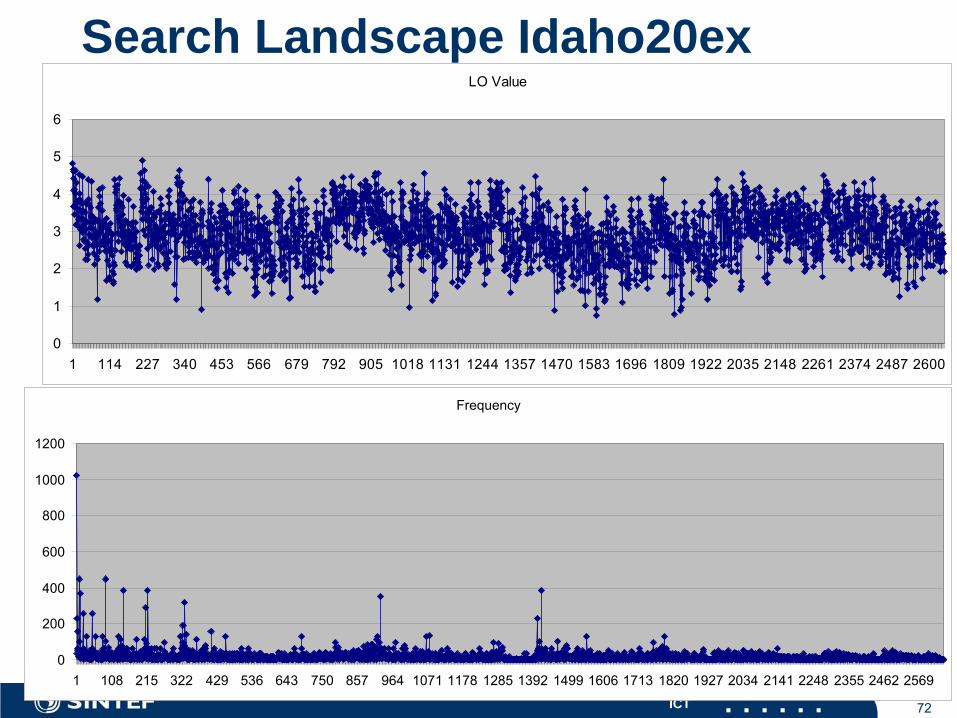
Search Landscape Idaho20ex
Frequency
0
200
400
600
800
1000
1200
1 108 215 322 429 536 643 750 857 964 1071 1178 1285 1392 1499 1606 1713 1820 1927 2034 2141 2248 2355 2462 2569
LO Value
0
1
2
3
4
5
6
1 114 227 340 453 566 679 792 905 1018 1131 1244 1357 1470 1583 1696 1809 1922 2035 2148 2261 2374 2487 2600
73ICT
Geir Hasle - eVITA Winter School 2009
Local SearchOld idea, new developments over the past two decadesPopular method for solving hard DOPsGeneric and flexibleNo strong assumptions
”Anytime”-methodEfficient, good quality solution quicklyPerformance depending on initial solution, neighborhood operator and strategy
Exact methods preferable, if they solve the problem
74ICT
Geir Hasle - eVITA Winter School 2009
Local Search
The search landscape is typically complexLocal optima may be far from global optimaLocal search is a local methodSolution quality depends on initial solution, neighborhood, strategy
”Blind” and ”headstrong” method, no learning during search, norandomness
No strong performance guarantees

75ICT
Geir Hasle - eVITA Winter School 2009
What
to do to move
on
from a local optimum to cover a larger
part of
the
search
space?
76ICT
Geir Hasle - eVITA Winter School 2009
How to escape local optima in LS - some strategies
RestartRandom choice of moveAllow moves to lower quality solutions
deterministicprababilistic
Memorywhich solutions have been visited before?diversify the search(parts of) good solutionsintensify the search
Change the search landscapeChange neighborhoodChange evaluation function
77ICT
Geir Hasle - eVITA Winter School 2009
Metaheuristics (General heuristics)
search strategies that escape local optimaintroduced early 1980iesconsiderable success in solving hard DOPsanalogies from physics, biology, human brain, human problem solvinga large number of variantssome religionssome confusion in the literature
78ICT
Geir Hasle - eVITA Winter School 2009
Some metaheuristicsSimulated Annealing (SA)Threshold Accepting (TA)Genetic Algorithms (GA) Memetic Algorithms (MA)Evolutionary Algorithms (EA)Differential Evolution (DE)Ant Colony Optimization (ACO)Particle Swarm Optimization (PSO)Immune Systems (IS)Tabu Search (TS)Scatter Search (SS)Path Relinking (PR)Guided Local Search (GLS)Greedy Randomized Adaptive Search (GRASP)Iterated Local Search (ILS)Very Large Neighborhood Search (VLNS)Variable Neighborhood Descent / Search (VND/VNS)Neural Networks (NN)
79ICT
Geir Hasle - eVITA Winter School 2009
”Definition” of metaheuristics (Osman & Kelly)
A metaheuristic is an iterative generation
process
that
guides an underlying
heuristicby combining
(in an intelligent way) different
strategies
for exploring
and exploiting
solution
spaces
(and learning
strategies) to find
near-optimal
solutions
in an effective
way
80ICT
Geir Hasle - eVITA Winter School 2009
”Definition” of metaheuristics (Glover & Kochenberger)
Solution
methods
that
utilize
interaction between
local improvement procedures (local
search) and higher
level
strategies to escape local optima and ensure robust search in a solution
space
81ICT
Geir Hasle - eVITA Winter School 2009
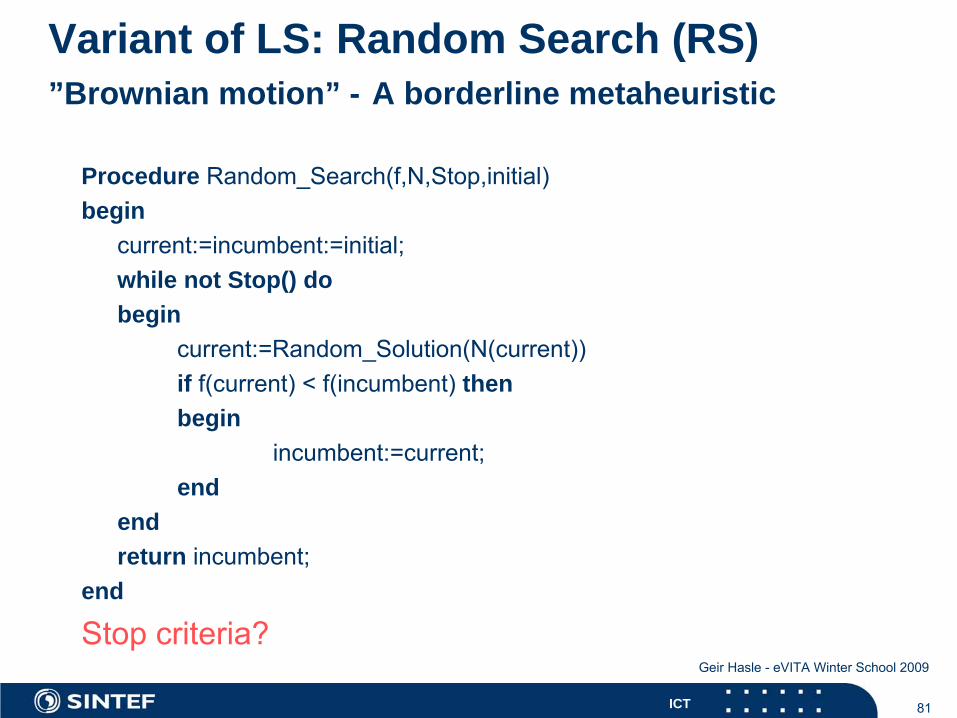
Variant of LS: Random Search (RS) ”Brownian motion” - A borderline metaheuristic
Procedure Random_Search(f,N,Stop,initial)begin
current:=incumbent:=initial;while not Stop() dobegin
current:=Random_Solution(N(current))if f(current) < f(incumbent) thenbegin
incumbent:=current;end
endreturn incumbent;
end
Stop
criteria?
82ICT
Geir Hasle - eVITA Winter School 2009
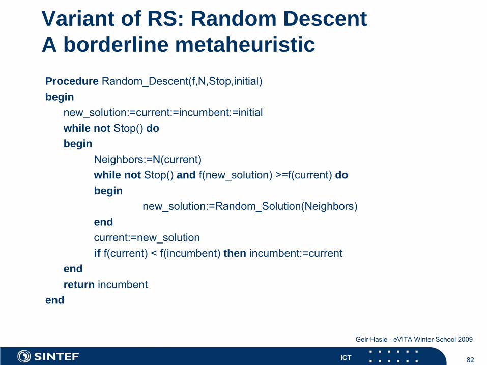
Variant of RS: Random Descent A borderline metaheuristicProcedure Random_Descent(f,N,Stop,initial)begin
new_solution:=current:=incumbent:=initialwhile not Stop() dobegin
Neighbors:=N(current)while not Stop()
and f(new_solution) >=f(current)
dobegin
new_solution:=Random_Solution(Neighbors)endcurrent:=new_solutionif f(current) < f(incumbent) then incumbent:=current
endreturn incumbent
end

83ICT
Geir Hasle - eVITA Winter School 2009
Metaheuristic strategies
Goalsescape local optimaavoid loops
Accept worse solutionsRandomness
Simulated Annealing (SA) utilizes these strategies
84ICT
Geir Hasle - eVITA Winter School 2009
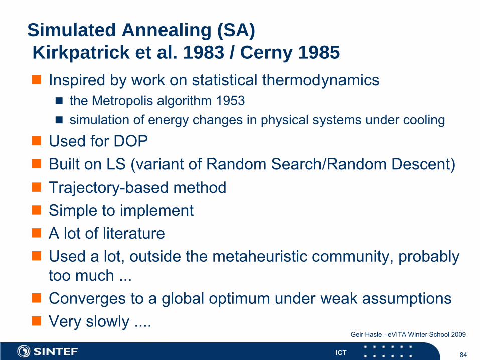
Simulated Annealing (SA) Kirkpatrick et al. 1983 / Cerny 1985
Inspired by work on statistical thermodynamicsthe Metropolis algorithm 1953simulation of energy changes in physical systems under cooling
Used for DOPBuilt on LS (variant of Random Search/Random Descent)Trajectory-based methodSimple to implementA lot of literatureUsed a lot, outside the metaheuristic community, probablytoo much ... Converges to a global optimum under weak assumptionsVery slowly ....
85ICT
Geir Hasle - eVITA Winter School 2009
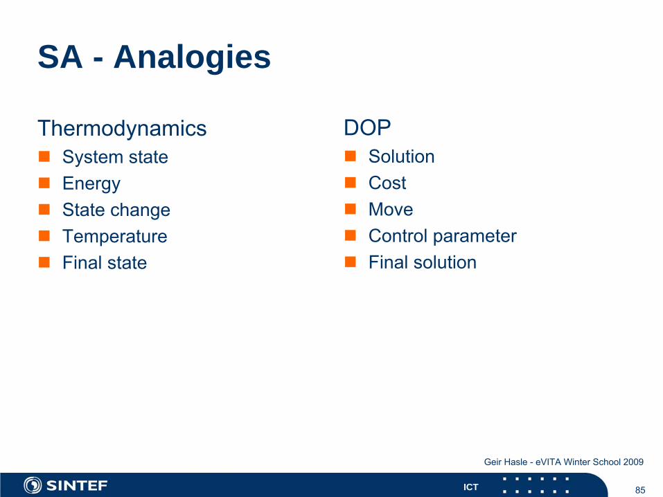
SA - Analogies
ThermodynamicsSystem stateEnergyState changeTemperatureFinal state
DOPSolutionCostMoveControl parameterFinal solution
86ICT
Geir Hasle - eVITA Winter School 2009
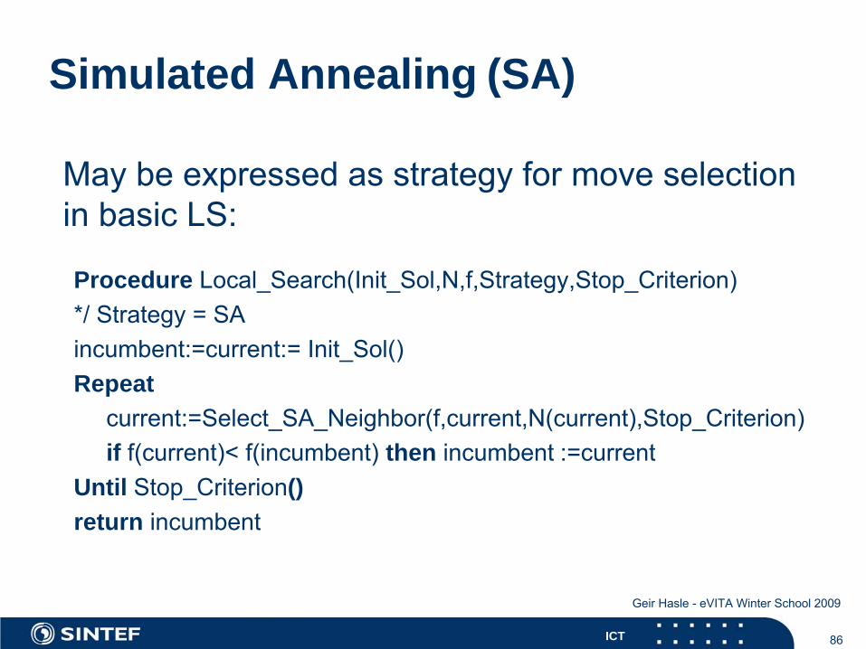
Simulated Annealing (SA)
Procedure Local_Search(Init_Sol,N,f,Strategy,Stop_Criterion)*/ Strategy
= SA
incumbent:=current:= Init_Sol()Repeat
current:=Select_SA_Neighbor(f,current,N(current),Stop_Criterion)if f(current)< f(incumbent) then incumbent
:=current
Until Stop_Criterion()return incumbent
May be expressed
as strategy
for move
selectionin basic
LS:
87ICT
Geir Hasle - eVITA Winter School 2009
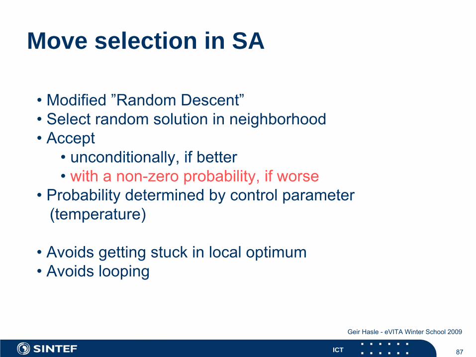
Move selection in SA
• Modified
”Random
Descent”• Select
random
solution
in neighborhood
• Accept• unconditionally, if
better
• with
a non-zero
probability, if
worse•
Probability
determined
by control
parameter
(temperature)
• Avoids
getting
stuck
in local
optimum• Avoids
looping
88ICT
Geir Hasle - eVITA Winter School 2009
Move selection in SA
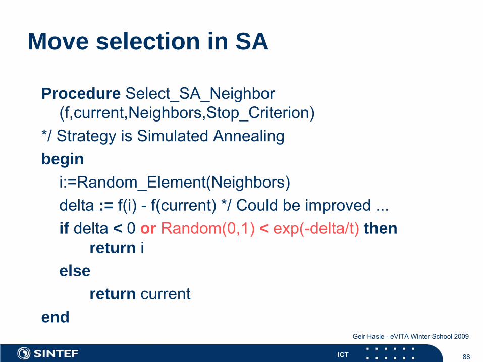
Procedure Select_SA_Neighbor (f,current,Neighbors,Stop_Criterion)
*/ Strategy
is Simulated
Annealingbegin
i:=Random_Element(Neighbors)delta
:= f(i) -
f(current) */ Could
be improved
...
if delta
< 0 or Random(0,1)
< exp(-delta/t)
then return i
elsereturn current
end
89ICT
Geir Hasle - eVITA Winter School 2009
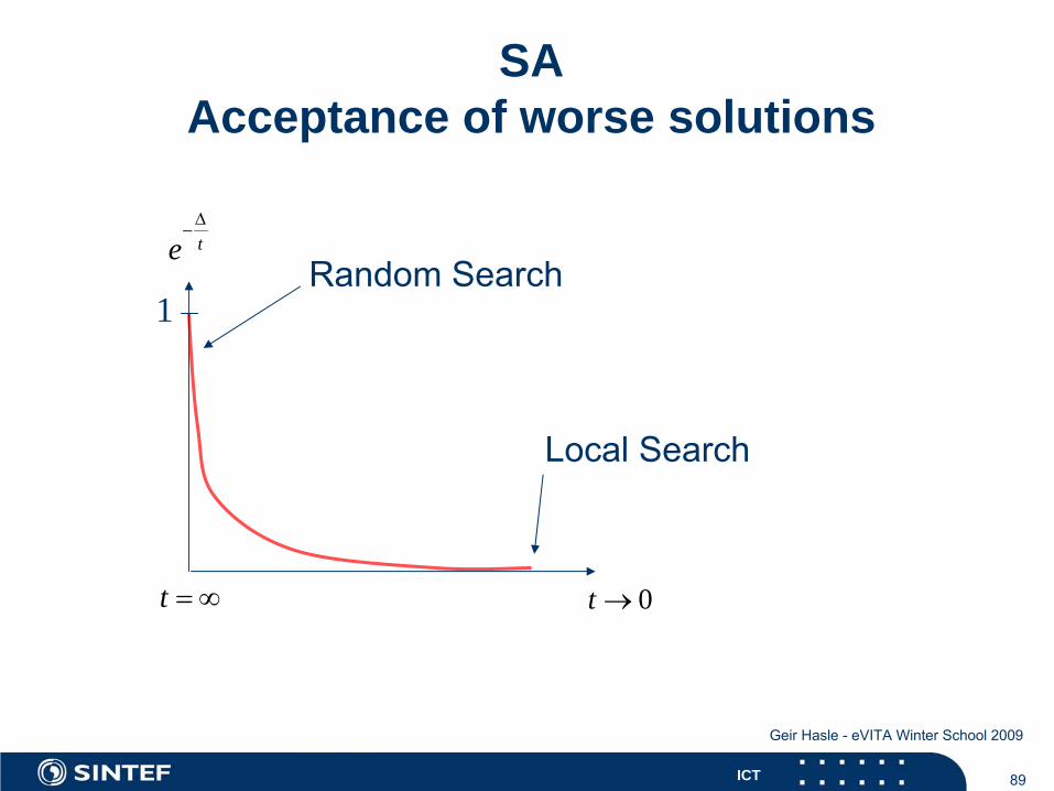
SA Acceptance of worse solutions
Random
Search
Local
Search
t = ∞
teΔ
−
0t →
1
90ICT
Geir Hasle - eVITA Winter School 2009
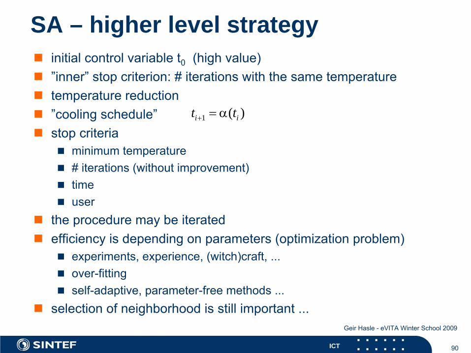
SA – higher level strategyinitial control variable t0 (high value)”inner” stop criterion: # iterations with the same temperaturetemperature reduction”cooling schedule”stop criteria
minimum temperature# iterations (without improvement)timeuser
the procedure may be iteratedefficiency is depending on parameters (optimization problem)
experiments, experience, (witch)craft, ...over-fittingself-adaptive, parameter-free methods ...
selection of neighborhood is still important ...
1 ( )i it t+ = α

91ICT
Geir Hasle - eVITA Winter School 2009
SA – overall procedureProcedure Simulated_Annealing
(f,N,Stop_Criterion,t0,Nrep,Cool)incumbent:=current:= Find_Initial_Solution()t:=t0Repeat
for i:=1
to Nrep
do */ Several
iterations
with
one
t valuebegin
current
:=Select_SA_Neighbor(f, current,N(sol),incumbent,t)if
f(current) < f(incumbent) then incumbent:= current
end
t:=Cool(t)
*/ CoolingUntil Stop_Criterion()return incumbent
92ICT
Geir Hasle - eVITA Winter School 2009
Statistical analysis of SA
Model: state transitions in search spaceTransition probabilities [pij], only dependent on statesHomogeneous Markov chain
When all transition probabilities are finite, SA will converge to a stationary distributionthat is independent of the initial solution. When the temperature goes tozero, the distribution converges to a uniform distribution overthe global optima.
Statistical guaranteeIn practice: exponential computing time needed to guarantee optimum
93ICT
Geir Hasle - eVITA Winter School 2009
SA i practice
heuristic approximation algorithmperformance strongly dependent on cooling schedulerules of thumb
large # iterations, few temperaturessmall # iterations, many temperatures

94ICT
Geir Hasle - eVITA Winter School 2009
SA in practice – Cooling schedule
geometric sequence often works well
1 , 0, , 1 (0.8 0.99)i it at i K a+ = = < −…
vary # repetitions and a, adaptationcomputational experiments
95ICT
Geir Hasle - eVITA Winter School 2009
SA – Cooling schedule
# repetitions and reduction rate should reflect search landscape Tuned to maximum difference between solution valuesAdaptive # repetitions
more repetitions for lower temperaturesacceptance rate, maximum limit
Very low temperatures are unnecessary (Local Search)Overall cooling rate more important than the specific cooling function

96ICT
Geir Hasle - eVITA Winter School 2009
SA – Decisions
Goal: High quality solution in short timeSearch space: only feasible solutions?NeighborhoodEvaluation functionCooling schedule
97ICT
Geir Hasle - eVITA Winter School 2009
SA – Computational efficiency aspects
Random choice of neighborneighborhood reduction, good candidates
Evaluation of objective (evaluation function)difference without full calculationapproximation
Evaluation of constraints (evaluation function)Move acceptance
calculating the exponential function takes timedrawing random numbers take time
Parallel computingfine-grained, in Local Searchcoarse-grained: multiple SA searches
98ICT
Geir Hasle - eVITA Winter School 2009
SA – Modifications and extensions
ProbabilisticAcceptance probabilityApproximation of (exponential) function / tableApproximation of cost functionFew temperaturesRestart
DeterministicThreshold Accepting (TA), Dueck and Scheuer 1990Record-to-Record Travel (RTR), The Great DelugeAlgorithm (GDA), Dueck 1993
99ICT
Geir Hasle - eVITA Winter School 2009
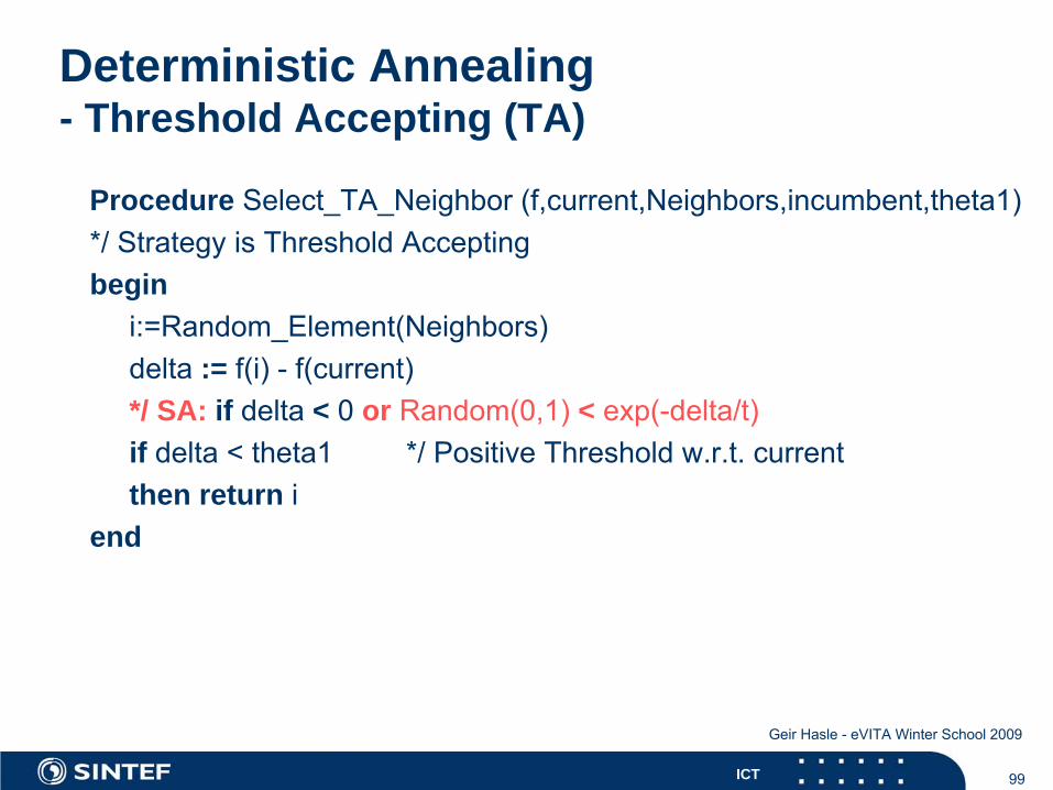
Deterministic Annealing - Threshold Accepting (TA)
Procedure Select_TA_Neighbor
(f,current,Neighbors,incumbent,theta1)*/ Strategy
is Threshold
Accepting
begini:=Random_Element(Neighbors)delta
:= f(i) -
f(current)
*/ SA: if delta
< 0 or Random(0,1)
< exp(-delta/t)if delta < theta1 */ Positive Threshold
w.r.t. current
then return iend
100ICT
Geir Hasle - eVITA Winter School 2009
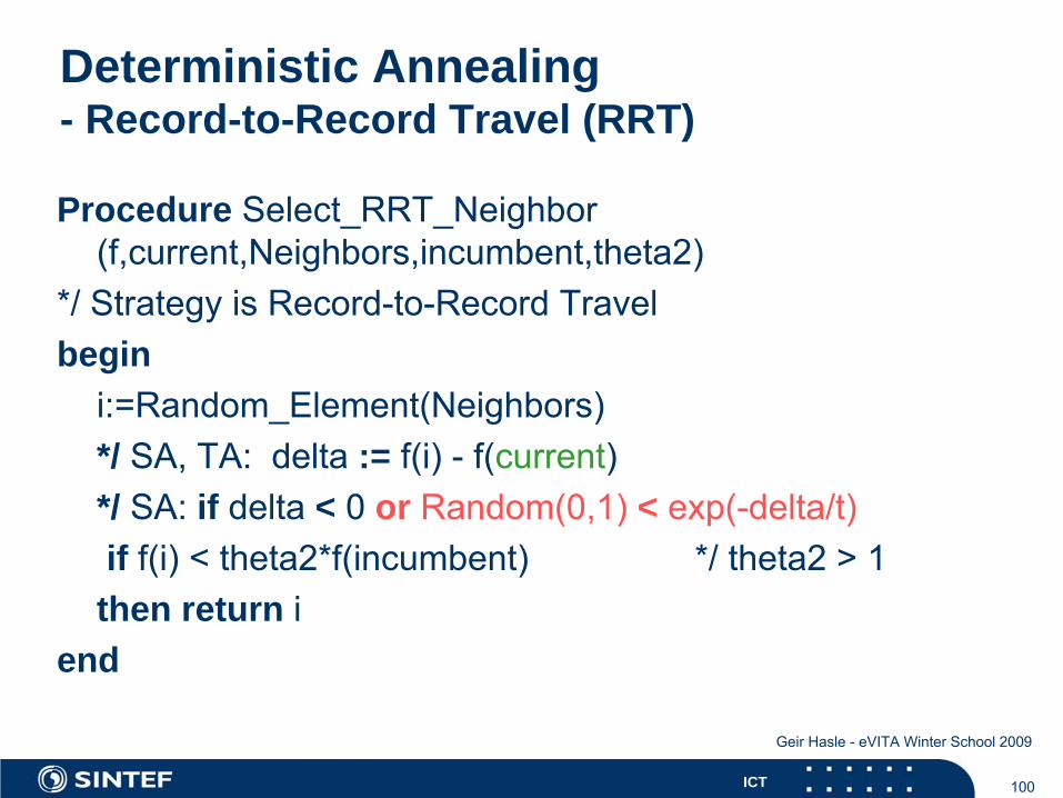
Deterministic Annealing - Record-to-Record Travel (RRT)
Procedure Select_RRT_Neighbor (f,current,Neighbors,incumbent,theta2)
*/ Strategy
is Record-to-Record
Travelbegin
i:=Random_Element(Neighbors)*/ SA, TA: delta
:= f(i) -
f(current)
*/ SA:
if delta
< 0 or Random(0,1)
< exp(-delta/t)if f(i) < theta2*f(incumbent) */ theta2 > 1then return i
end
101ICT
Geir Hasle - eVITA Winter School 2009
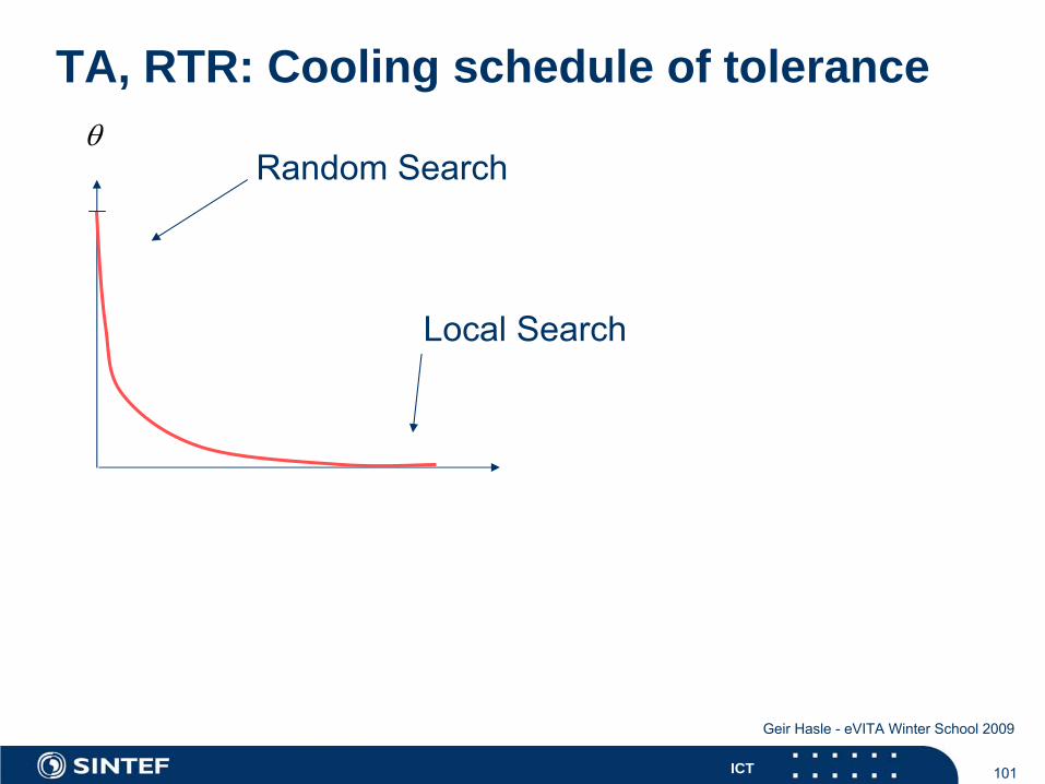
TA, RTR: Cooling schedule of tolerance
Random
Search
Local
Search
θ
102ICT
Geir Hasle - eVITA Winter School 2009
Tabu Search (TS) F. Glover / P. Hansen 1986
Fred Glover 1986: ”Future paths for integer programming and links to artificial intelligence”Pierre Hansen 1986: ”The Steepest Ascent/Mildest Descent Heuristicfor Combinatorial Optimization”DOP research – OR and AIBarrier methods, search in infeasible spaceSurrogate constraintsCutting plane methodsAutomated learning, cognitive science
103ICT
Geir Hasle - eVITA Winter School 2009
Tabu (Taboo)
”Banned
because
of
moral, taste, or risk”Tabu Search: Search
guidance
towards
otherwise
inaccessible
areas of
the
search
space
by use
of
restrictions
Principles for intelligent problem solvingStructures that exploit history (”learning”)
104ICT
Geir Hasle - eVITA Winter School 2009
Tabu Search – Main ideas
Trajectory-based method, based on Local SearchSeeks to allow local optima by allowing non-improving movesAggressive: Always move to best solution in neighborhoodLooping problem, particularly for symmetric neighborhoodsUse of memory to
avoid loops (short term memory) diversify the search (long term memory) intensify the search (long term memory) General strategy to control ”inner” heuristics (LS, ...)
Metaheuristic (Glover)
105ICT
Geir Hasle - eVITA Winter School 2009
Basic Tabu Search
LS with ”Best Neighbor” strategyAlways move to new neighbor (”aggressive LS”)But: some neighbors are tabuTabu status defined by tabu-criteriaHowever: some tabu moves are admissible
admissibility criteriatypical example: new incumbent
Short term memory: Tabu List
106ICT
Geir Hasle - eVITA Winter School 2009
Tabu Restrictions
defined on properties of solutions or moves – attributeshow often – or how recent (frequency, recency) has theattribute been involved in (generating) a solutiondata structure: tabu list
107ICT
Geir Hasle - eVITA Winter School 2009
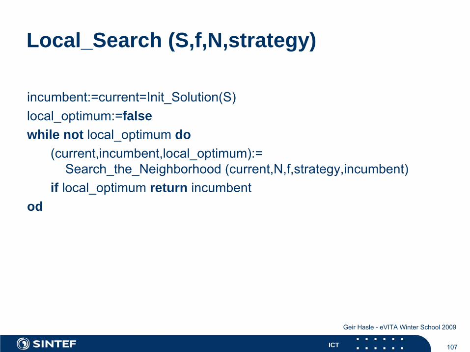
Local_Search (S,f,N,strategy)
incumbent:=current=Init_Solution(S)local_optimum:=falsewhile not local_optimum
do
(current,incumbent,local_optimum):= Search_the_Neighborhood
(current,N,f,strategy,incumbent)
if local_optimum
return incumbentod
108ICT
Geir Hasle - eVITA Winter School 2009
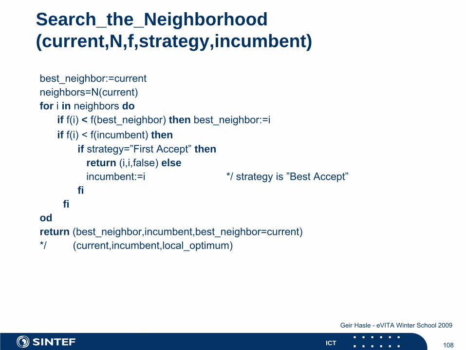
Search_the_Neighborhood (current,N,f,strategy,incumbent)
best_neighbor:=currentneighbors=N(current)for i
in neighbors
doif f(i)
< f(best_neighbor)
then best_neighbor:=iif f(i) < f(incumbent) then
if strategy=”First
Accept”
thenreturn (i,i,false) elseincumbent:=i
*/ strategy
is ”Best Accept”fi
fiodreturn (best_neighbor,incumbent,best_neighbor=current)*/ (current,incumbent,local_optimum)

109ICT
Geir Hasle - eVITA Winter School 2009
Traversing the Neighborhood Graph
1 ( ), 0,k ks N s k+ σ∈ = …
0s 1s
0( )N sσ
1s
0s
1( )N sσ
2s1s
A move
is
the
process
of
selecting
a given solution
in the
neighborhood
of
the
current
solution, hence
making it the
current
solution
for the
next
iteration
110ICT
Geir Hasle - eVITA Winter School 2009
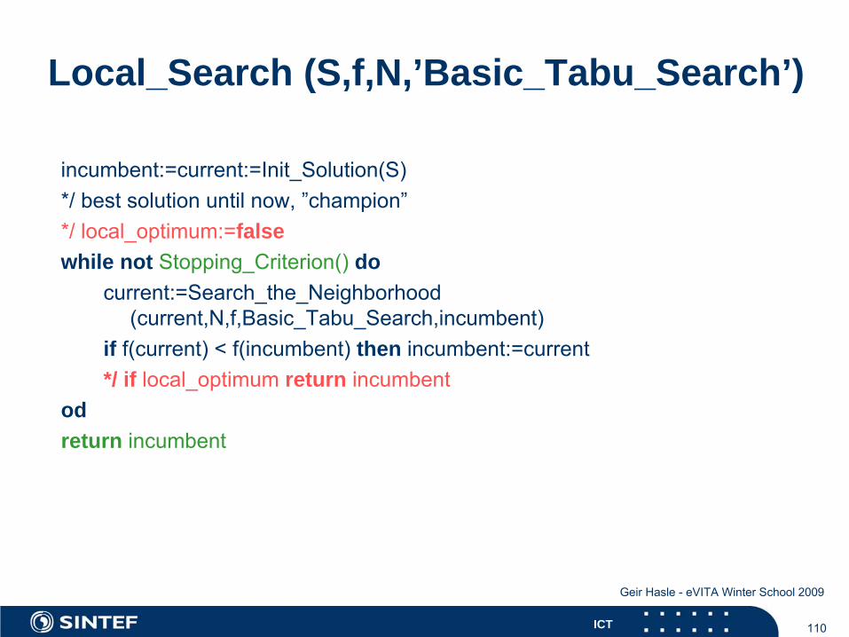
Local_Search (S,f,N,’Basic_Tabu_Search’)
incumbent:=current:=Init_Solution(S)*/ best solution
until
now, ”champion”
*/ local_optimum:=falsewhile not Stopping_Criterion()
do
current:=Search_the_Neighborhood (current,N,f,Basic_Tabu_Search,incumbent)
if f(current) < f(incumbent) then incumbent:=current*/ if local_optimum
return incumbent
odreturn incumbent
111ICT
Geir Hasle - eVITA Winter School 2009
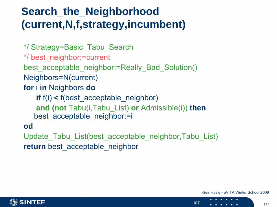
Search_the_Neighborhood (current,N,f,strategy,incumbent)
*/ Strategy=Basic_Tabu_Search*/ best_neighbor:=currentbest_acceptable_neighbor:=Really_Bad_Solution()Neighbors=N(current) for i
in Neighbors
do
if f(i)
< f(best_acceptable_neighbor)and (not Tabu(i,Tabu_List)
or Admissible(i))
then
best_acceptable_neighbor:=iodUpdate_Tabu_List(best_acceptable_neighbor,Tabu_List)return best_acceptable_neighbor
112ICT
Geir Hasle - eVITA Winter School 2009
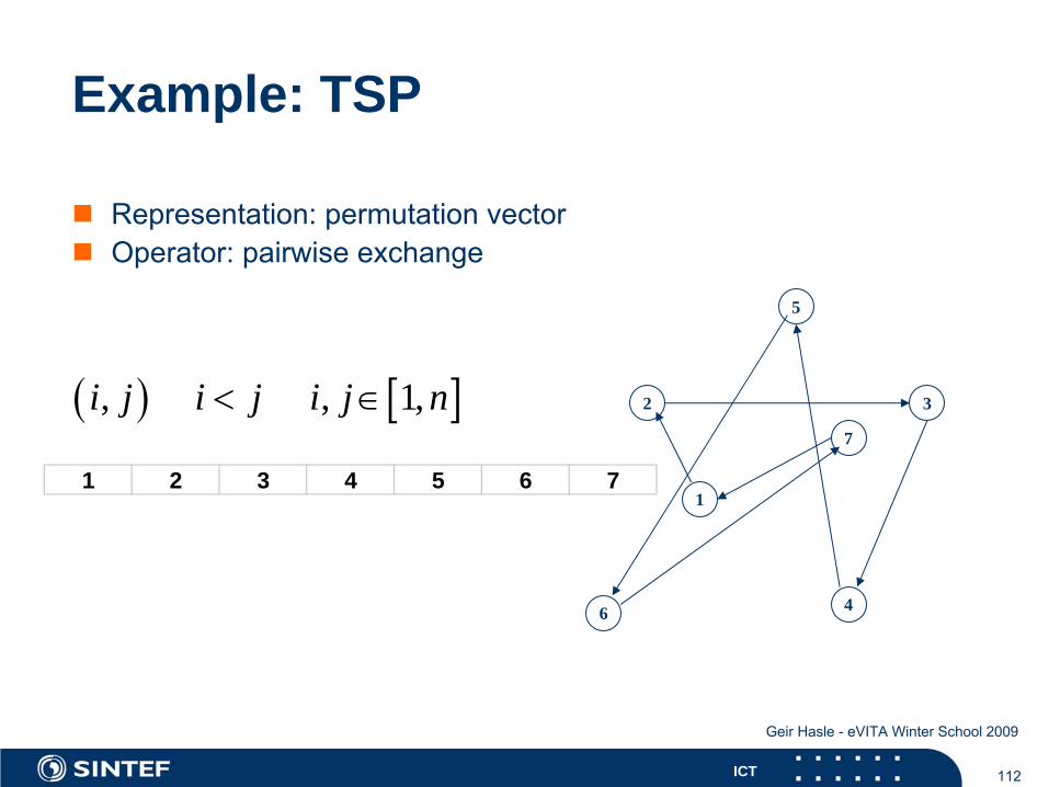
Example: TSP
Representation: permutation vectorOperator: pairwise exchange
4
1
6
5
7
2 3
1 2 3 4 5 6 7
( ) [ ], , 1,i j i j i j n< ∈
113ICT
Geir Hasle - eVITA Winter School 2009
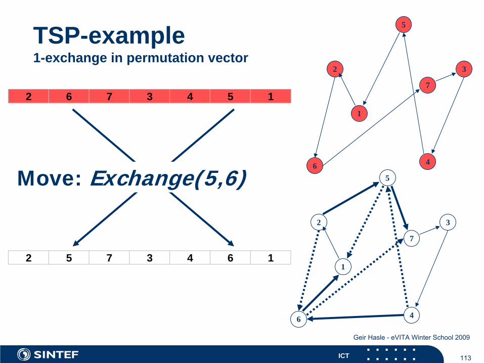
TSP-example 1-exchange in permutation vector
4
1
6
5
7
2 3
2 5 7 3 4 6 1
2 6 7 3 4 5 1
4
1
6
5
7
2 3
Move: Exchange(5,6)
114ICT
Geir Hasle - eVITA Winter School 2009
TSP-example 1-exchange
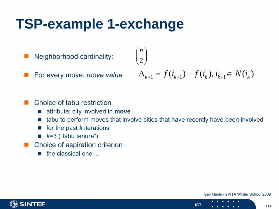
Neighborhood cardinality:
For every move: move value
Choice of tabu restrictionattribute: city involved in movetabu to perform moves that involve cities that have recently have been involvedfor the past k iterationsk=3 (”tabu tenure”)
Choice of aspiration criterionthe classical one ...
2n⎛ ⎞⎜ ⎟⎝ ⎠
1 1 1( ) ( ), ( )k k k k kf i f i i N i+ + +Δ = − ∈
115ICT
Geir Hasle - eVITA Winter School 2009
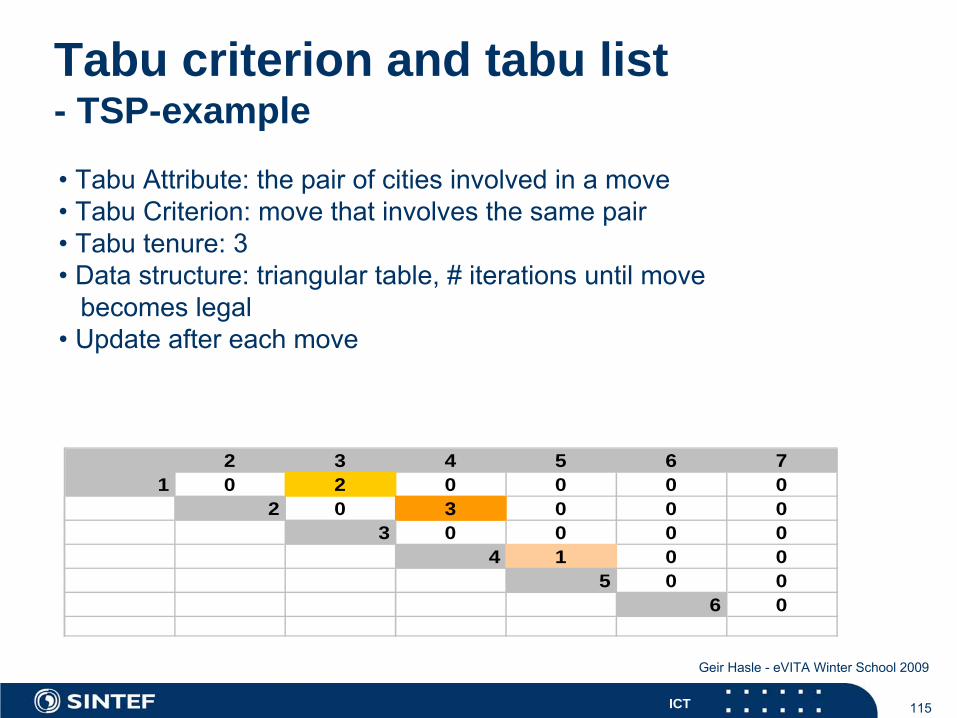
Tabu criterion and tabu list - TSP-example
• Tabu Attribute: the
pair of
cities
involved
in a move• Tabu Criterion: move
that
involves
the
same pair
• Tabu tenure: 3•
Data structure: triangular
table, # iterations
until
move
becomes
legal• Update
after
each
move
2 3 4 5 6 71 0 2 0 0 0 0
2 0 3 0 0 03 0 0 0 0
4 1 0 05 0 0
6 0
116ICT
Geir Hasle - eVITA Winter School 2009
Alternative tabu criteria / attributes - TSP-example
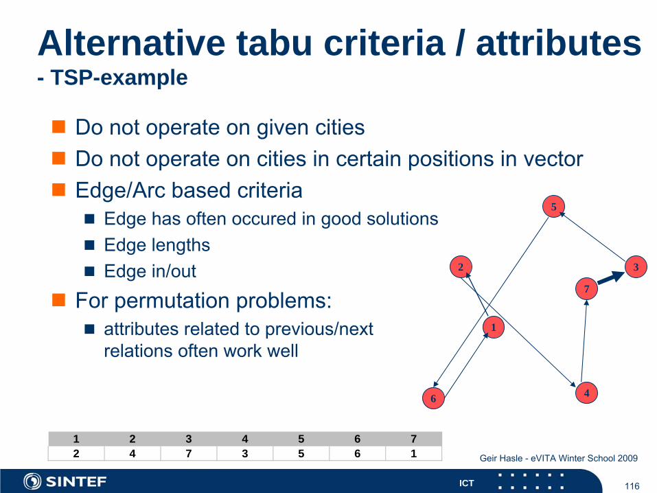
1 2 3 4 5 6 72 4 7 3 5 6 1
4
1
6
5
7
2 3
Do not operate on given citiesDo not operate on cities in certain positions in vectorEdge/Arc based criteria
Edge has often occured in good solutionsEdge lengthsEdge in/out
For permutation problems:attributes related to previous/nextrelations often work well
117ICT
Geir Hasle - eVITA Winter School 2009
Candidate list of moves - TSP-example
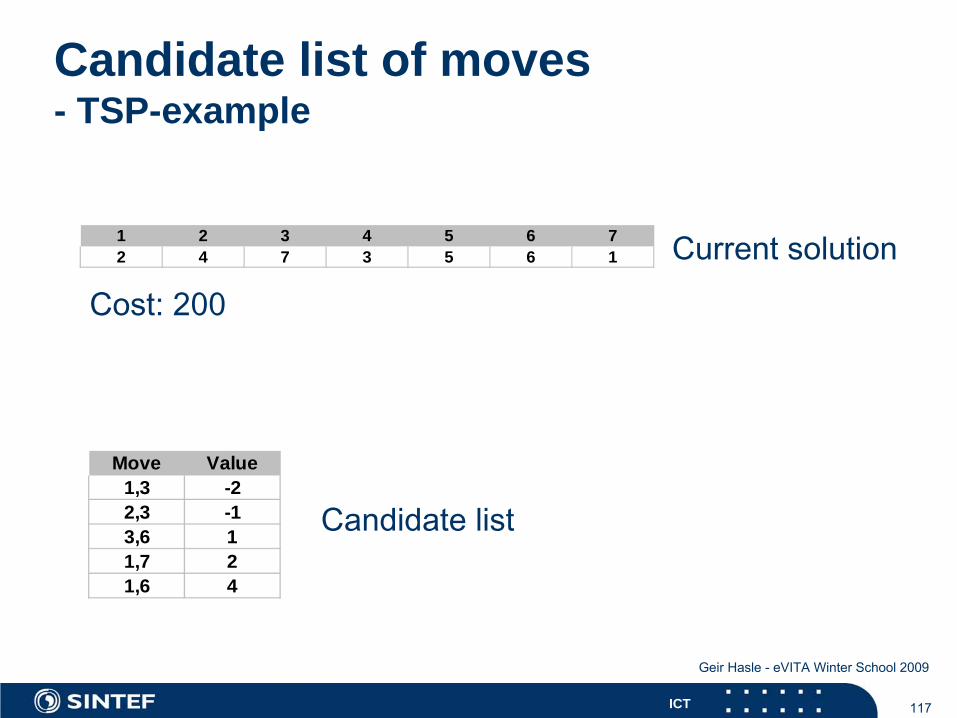
1 2 3 4 5 6 72 4 7 3 5 6 1 Current
solution
Move Value1,3 -22,3 -13,6 11,7 21,6 4
Cost: 200
Candidate
list
118ICT
Geir Hasle - eVITA Winter School 2009
TSP-example 1-exchange - Iteration 0/1
Tabu list 2 3 4 5 6 71 0 0 0 0 0 0
2 0 0 0 0 03 0 0 0 0
4 0 0 05 0 0
6 0
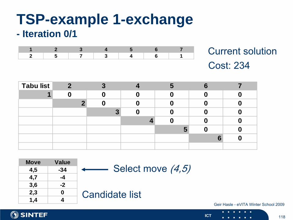
1 2 3 4 5 6 72 5 7 3 4 6 1 Current
solution
Cost: 234
Move Value4,5 -344,7 -43,6 -22,3 01,4 4
Candidate
list
Select
move (4,5)
119ICT
Geir Hasle - eVITA Winter School 2009
TSP-example - Iteration 1 (after Exchange (4,5))
Tabu list 2 3 4 5 6 71 0 0 0 0 0 0
2 0 0 0 0 03 0 0 0 0
4 3 0 05 0 0
6 0
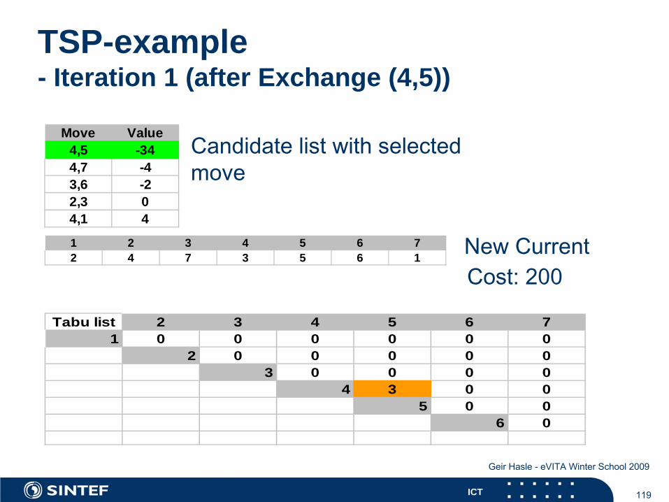
1 2 3 4 5 6 72 4 7 3 5 6 1 New Current
Cost: 200
Move Value4,5 -344,7 -43,6 -22,3 04,1 4
Candidate
list with
selected move
120ICT
Geir Hasle - eVITA Winter School 2009
TSP-example - Iteration 2
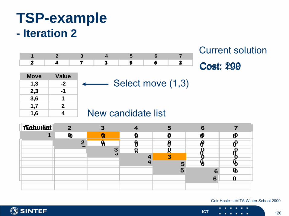
Tabu list 2 3 4 5 6 71 0 3 0 0 0 0
2 0 0 0 0 03 0 0 0 0
4 2 0 05 0 0
6 0
Tabu list 2 3 4 5 6 71 0 0 0 0 0 0
2 0 0 0 0 03 0 0 0 0
4 3 0 05 0 0
6 0
1 2 3 4 5 6 72 4 7 3 5 6 1
Current
solutionCost: 200
Move Value1,3 -22,3 -13,6 11,7 21,6 4 New candidate
list
Select
move
(1,3)
1 2 3 4 5 6 72 4 7 1 5 6 3 Cost: 198
121ICT
Geir Hasle - eVITA Winter School 2009
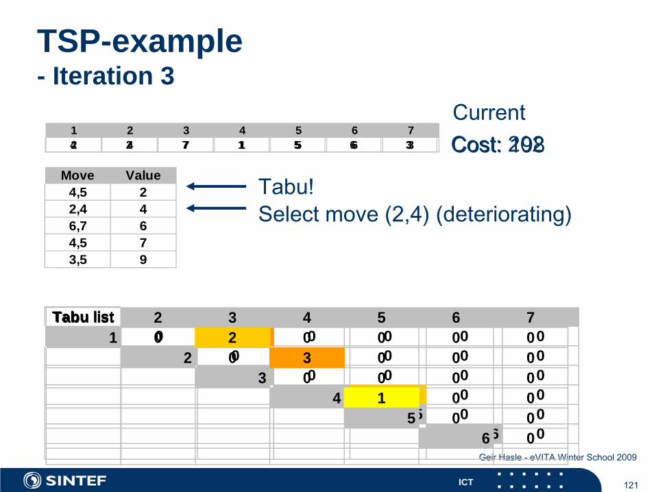
TSP-example - Iteration 3
1 2 3 4 5 6 74 2 7 1 5 6 3
Tabu list 2 3 4 5 6 71 0 3 0 0 0 0
2 0 0 0 0 03 0 0 0 0
4 2 0 05 0 0
6 0
1 2 3 4 5 6 72 4 7 1 5 6 3
CurrentCost: 198
Select
move
(2,4) (deteriorating)Tabu!Move Value
4,5 22,4 46,7 64,5 73,5 9
Cost: 202
Tabu list 2 3 4 5 6 71 0 2 0 0 0 0
2 0 3 0 0 03 0 0 0 0
4 1 0 05 0 0
6 0
122ICT
Geir Hasle - eVITA Winter School 2009
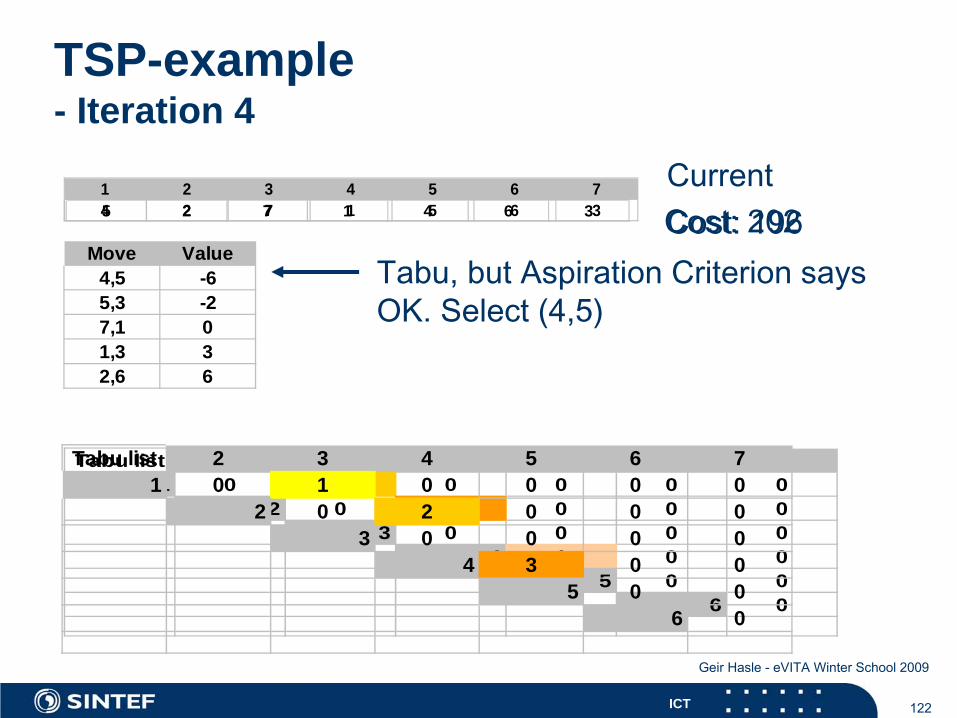
TSP-example - Iteration 4
1 2 3 4 5 6 75 2 7 1 4 6 3
Tabu list 2 3 4 5 6 71 0 2 0 0 0 0
2 0 3 0 0 03 0 0 0 0
4 1 0 05 0 0
6 0
1 2 3 4 5 6 74 2 7 1 5 6 3
CurrentCost: 202
Tabu, but
Aspiration
Criterion
says OK. Select
(4,5)
Move Value4,5 -65,3 -27,1 01,3 32,6 6
Cost: 196
Tabu list 2 3 4 5 6 71 0 1 0 0 0 0
2 0 2 0 0 03 0 0 0 0
4 3 0 05 0 0
6 0
123ICT
Geir Hasle - eVITA Winter School 2009
Observations
In the example 3 of 21 moves are tabuStronger tabu criteria are achieved by
increasing tabu tenurestrengthening the tabu restriction
Dynamic tabu tenure (“Reactive Tabu Search”) often works better than staticTabu-list requires space (why not store full solutions instead of attributes?) In the example: the tabu criterion is based on recency, short term memoryLong term memory: normally based on frequency

124ICT
Geir Hasle - eVITA Winter School 2009
TSP-example - Frequency based long term memory
1 2 3 4 5 6 71 22 33 34 1 5 15 4 46 1 27 4 3
Tabu status (recency)
Frequency of moves
Typically utilized to diversify search Is often activated when the search stagnates (no improving moves for a long time)Typical mechanism for long-term diversification strategies: Penalty for moves that have
been frequently usedAugmented move evaluation
125ICT
Geir Hasle - eVITA Winter School 2009
Tabu Search - Main IdeasLess use of randomization (than SA)“Intelligent” search must be based on more systematic guidanceEmphasis on flexible memory structuresNeighborhoods are in effect modified on the basis of short term memory (one excludes solutions that are tabu)Memory of good solutions (or parts of them), e.g. good local optima, particularly in long term strategiesUse of search history to modify evaluation of solutions/movesTS may be combined with penalties for constraint violations(a la Lagrange-relaxation) Strategic oscillation
intensification and diversificationfeasible space and infeasible space
126ICT
Geir Hasle - eVITA Winter School 2009
Tabu Search – More ideas, and practice
“Aggressive search”: move on – select good neighborComputational effort and scalability remedies (general)
delta-evaluationapproximation of cost functionidentify good candidates in neighborhood candidate list of moves, extensions
Most TS-implementations are deterministicProbabilistic Tabu Search
moves are chosen probabilistically, but based on TS principles
Most TS-implementations are simplebasic TS with short term memory, static tabu tenurepotential for improvement ...
127ICT
Geir Hasle - eVITA Winter School 2009
Tabu Search - Generic procedure
Find initial solution xInitialize memory HWhile not Stop_Criterion()
Find (with limited resources) Candidate_List_N(x) in N(x)Select (with limited resources) x’ = argmin(c(H,x), x in Candidate_List_N(x))x= x’H=Update(H)
end
128ICT
Geir Hasle - eVITA Winter School 2009
Tabu Search – Attributes
Attribute: Property of solution or moveMay be based on any aspect of the solution or moveBasis for definition of tabu restrictionsA move may change more than one attribute
129ICT
Geir Hasle - eVITA Winter School 2009
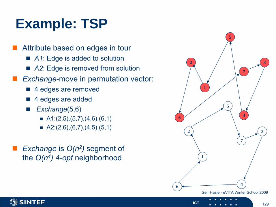
Example: TSPAttribute based on edges in tour
A1: Edge is added to solutionA2: Edge is removed from solution
Exchange-move in permutation vector:4 edges are removed4 edges are addedExchange(5,6)
A1:(2,5),(5,7),(4,6),(6,1)A2:(2,6),(6,7),(4,5),(5,1)
Exchange is O(n2) segment ofthe O(n4) 4-opt neighborhood
4
1
6
5
7
2 3
4
1
6
5
7
2 3
130ICT
Geir Hasle - eVITA Winter School 2009
Use of attributes in tabu restrictions
Assume that the move x(k)-> x(k+1) involves the attribute ANormal tabu restriction: Tabu to perform move that reverses the status of ATSP-example:
the attributes are edgescurrent move introduces edge (2,5): y2,5(0->1)moves that remove edge (2,5): y2,5(1->0) are tabu ( for some iterations)

131ICT
Geir Hasle - eVITA Winter School 2009
Tabu tenure – the (witch)craftStatic
t=7t=√n where n is a measure of problem size
Dynamic (and randomized)t ∈ [5,11]t ∈ [ .9√n, 1.1√n]
Depending on attributeTSPedge-attribute, tabu criterion both on edge in / edge outfewer edges in than out (n vs. n2-n)same tabu tenure would be unbalanced
Self-adaptation
132ICT
Geir Hasle - eVITA Winter School 2009
Aspiration criteriaClassical aspiration criterion: Accept tabu move that will give a new incumbentOther relevant criteria are based on:
solution qualitydegree of feasibilitystrength of tabudegree of change: Influence of move
High influence move may be important to follow when close to local optimum, search stagnates
Distance metrics for solutionsHamming-distance between strings
h(1011101,1001001) = 2 h(2173896,2233796) = 3 h("toned”,"roses”) = 3
More general, sequences: Edit Distance (Levenshtein) insertion, removal, transposition
133ICT
Geir Hasle - eVITA Winter School 2009
Frequency based memoryComplementary to short term memoryLong term strategiesFrequency measures
residence-basedtransition-based
TSP-examplehow often has a given edge (triplet, ...) been included in the current solution? (residence-based)how often has the in/out status of the edge been changed? (transition-based)
134ICT
Geir Hasle - eVITA Winter School 2009
Intensification and diversification
Intensification: Aggressive prioritization of good solution attributes
short term: based directly on attributeslong term: use of elite solutions, parts of elite solutions (vocabularies)
Diversification: Spreading of search, prioritization of moves that give solutions with new composition of attributes
Strategic oscillation
135ICT
Geir Hasle - eVITA Winter School 2009
Intensification and diversification - basic mechanisms
use of frequency based memoryselect solution from subset R of S (or X)diversification:
R is chosen to contain a large part of the solutions generated so far (e.g., all local optima)
intensification :R is chosen as a small set of elite solutions that
to a large degree have identical attributeshave a small distance in solution spacecluster analysispath relinking
136ICT
Geir Hasle - eVITA Winter School 2009
Path relinking
Assuming that new good solutions are found on the path between two good solutionsSelect two elite solutions x’ and x’’Find (shortest) path in the solution graph between them x’ -> x’(1)-> ... x’(r)= x’’Select one or more of the intermediate solutions as end points for path relinking
137ICT
Geir Hasle - eVITA Winter School 2009
Punishment and encouragement Whip and carrot
Augmented move evaluation, in addition to objectiveCarrot for intensification is whip for diversification, and viceversa
Diversificationmoves to solutions that have attributes with high frequency are penalizedTSP-example: g(x)=f(x)+w1Σωij
Intensificationmoves to solutions that have attributes that are frequent among elite solutions are encouragedTSP-example: g(x)=f(x)-w2Σγij
138ICT
Geir Hasle - eVITA Winter School 2009
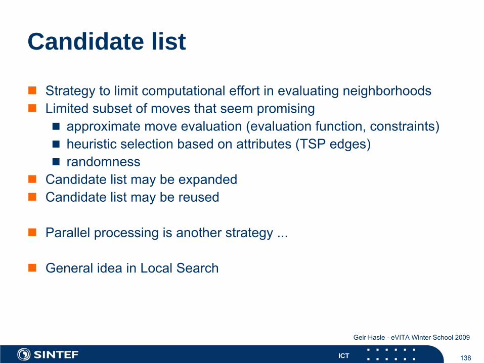
Candidate list
Strategy to limit computational effort in evaluating neighborhoodsLimited subset of moves that seem promising
approximate move evaluation (evaluation function, constraints) heuristic selection based on attributes (TSP edges)randomness
Candidate list may be expandedCandidate list may be reused
Parallel processing is another strategy ...
General idea in Local Search
139ICT
Geir Hasle - eVITA Winter School 2009
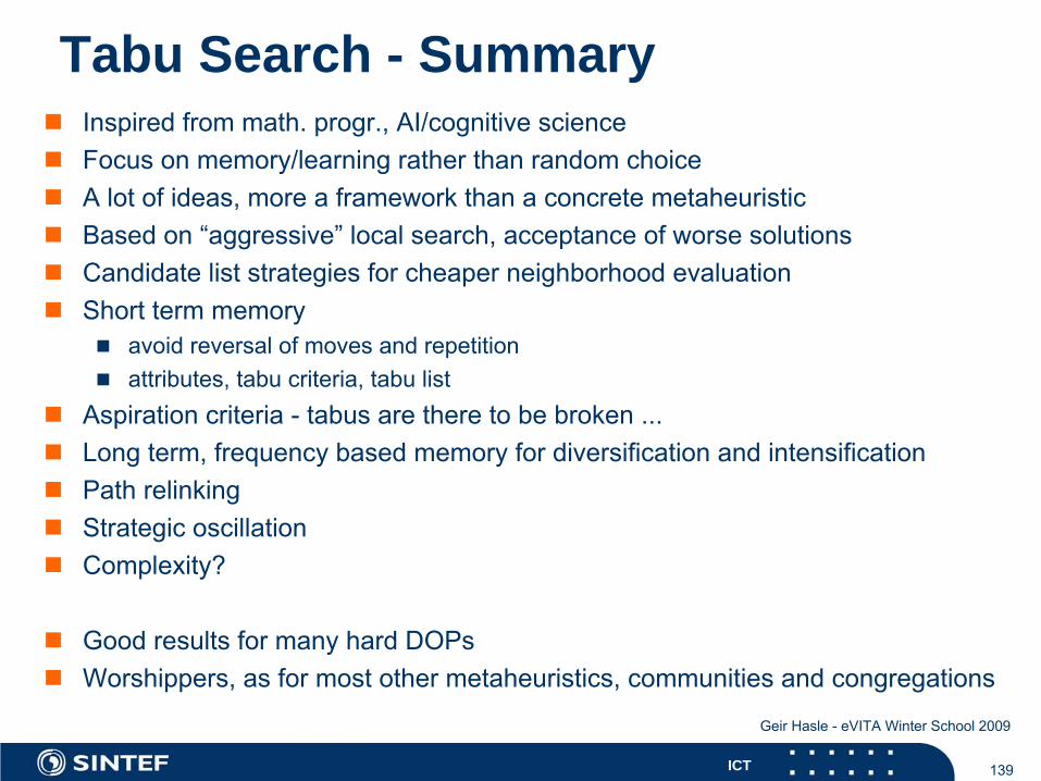
Tabu Search - SummaryInspired from math. progr., AI/cognitive scienceFocus on memory/learning rather than random choiceA lot of ideas, more a framework than a concrete metaheuristicBased on “aggressive” local search, acceptance of worse solutionsCandidate list strategies for cheaper neighborhood evaluationShort term memory
avoid reversal of moves and repetitionattributes, tabu criteria, tabu list
Aspiration criteria - tabus are there to be broken ...Long term, frequency based memory for diversification and intensificationPath relinkingStrategic oscillationComplexity?
Good results for many hard DOPsWorshippers, as for most other metaheuristics, communities and congregations
140ICT
Geir Hasle - eVITA Winter School 2009
Guided Local Search (GLS) (E. Tsang, C. Voudouris 1995)
Project for solving Constraint Satisfaction Problems (CSP), early 90ies(E. Tsang, C. Voudouris, A. Davenport)GENET (neural network)Development of GENET from CSP to ‘Partial CSP’satisfaction ⇒ optimizationthe Tunnelling Algorithm’ (94) -> GLS (95)
141ICT
Geir Hasle - eVITA Winter School 2009
GLS - Main ideasGeneral strategy for guidance of local search/”inner” heuristics: metaheuristic
Local search (trajectory based)
Penalizes undesired properties (‘features’) of solutions
Focuses on promising parts of the solution spaceSeeks to escape local optima through a dynamic, augmentedevaluation function (objective + penalty term)MemoryChanging the search landscapeLS to local minimum, update of penalty term, LS to localminimum, update of penalty term, ...
142ICT
Geir Hasle - eVITA Winter School 2009
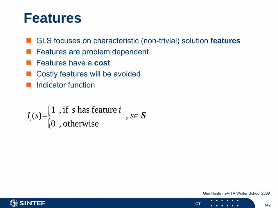
GLS focuses on characteristic (non-trivial) solution featuresFeatures are problem dependentFeatures have a costCostly features will be avoidedIndicator function
Features
1 , if has feature ( ) ,0 , otherwise
⎧⎪⎪⎨⎪⎪⎩
= ∈i
s iI s s S
143ICT
Geir Hasle - eVITA Winter School 2009
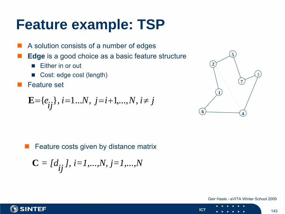
A solution consists of a number of edgesEdge is a good choice as a basic feature structure
Either in or outCost: edge cost (length)
Feature set
Feature example: TSP
{ }, 1... , 1,..., ,= = = + ≠e i N j i N i jijE
Feature costs given by distance matrix
= [d ], i=1,...,N, j=1,...,NijC
4
1
6
5
7
2
3
144ICT
Geir Hasle - eVITA Winter School 2009
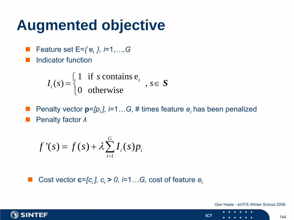
Feature set E={ ei }, i=1,…,GIndicator function
Augmented objective
Penalty vector p=[pi ], i=1…G, # times feature ei has been penalizedPenalty factor λ
1'( ) ( ) ( )
G
i ii
f s f s I s pλ=
= + ∑
1 if contains e( ) ,
0 otherwise⎧
= ∈⎨⎩
ii
sI s s S
Cost vector c=[ci ], ci > 0, i=1…G, cost of feature ei
145ICT
Geir Hasle - eVITA Winter School 2009
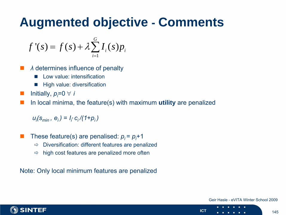
Augmented objective - Comments
1'( ) ( ) ( )
G
i ii
f s f s I s pλ=
= + ∑
λ determines influence of penaltyLow value: intensificationHigh value: diversification
Initially, pi=0 ∀ iIn local minima, the feature(s) with maximum utility are penalized
ui(smin , ei ) = Ii* ci /(1+pi )
These feature(s) are penalised: pi = pi+1Diversification: different features are penalizedhigh cost features are penalized more often
Note: Only
local
minimum features are
penalized
146ICT
Geir Hasle - eVITA Winter School 2009
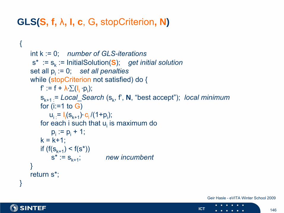
{int
k := 0; // number
of
GLS-iterations
s* := sk
:= InitialSolution(S); // get
initial solutionset
all pi
:= 0; // set
all penalties
to zerowhile
(stopCriterion
not satisfied) do {
f’
:= f + λ*
∑(Ii
*
pi
);sk+1 :
= Local_Search
(sk
, f’, N,
“best accept”); local
minimumfor (i:=1 to G)
ui :
= Ii
(sk+1
)* ci
/(1+pi
);for each
i such
that
ui
is maximum
dopi
:= pi
+ 1;k = k+1;if
(f(sk+1
) < f(s*))s* := sk+1
; // save new
incumbent}return
s*;
}
GLS(S, f, λ, I, c, G, stopCriterion, N)
147ICT
Geir Hasle - eVITA Winter School 2009
CommentsAugmented objective in Local Search
sk+1 := Local_Search (sk, f’, N, “best accept”);Local Search strategy may well be ”first accept”, ..Variants of Local_Search may be usedDelta-evaluation of moves must take penalties into accountIf all features are penalized equally many times f’(s) gives the same landscape as f(s)Resetting penalty vectors
Avoids bad features, how about encouragement of good features?
148ICT
Geir Hasle - eVITA Winter School 2009
λ
ValuesGLS seems to be rather robust regarding λ valuesGeneral advice: fraction of value of local minimumTsang & Voudouris:
TSP : λ = a*f(smin)/n , a∈[0,1] problem dependentQAP: λ = a*f(smin)/n2 , a∈[0.2,1] problem dependentFor other problems they report absolute values depending onproblem size
149ICT
Geir Hasle - eVITA Winter School 2009
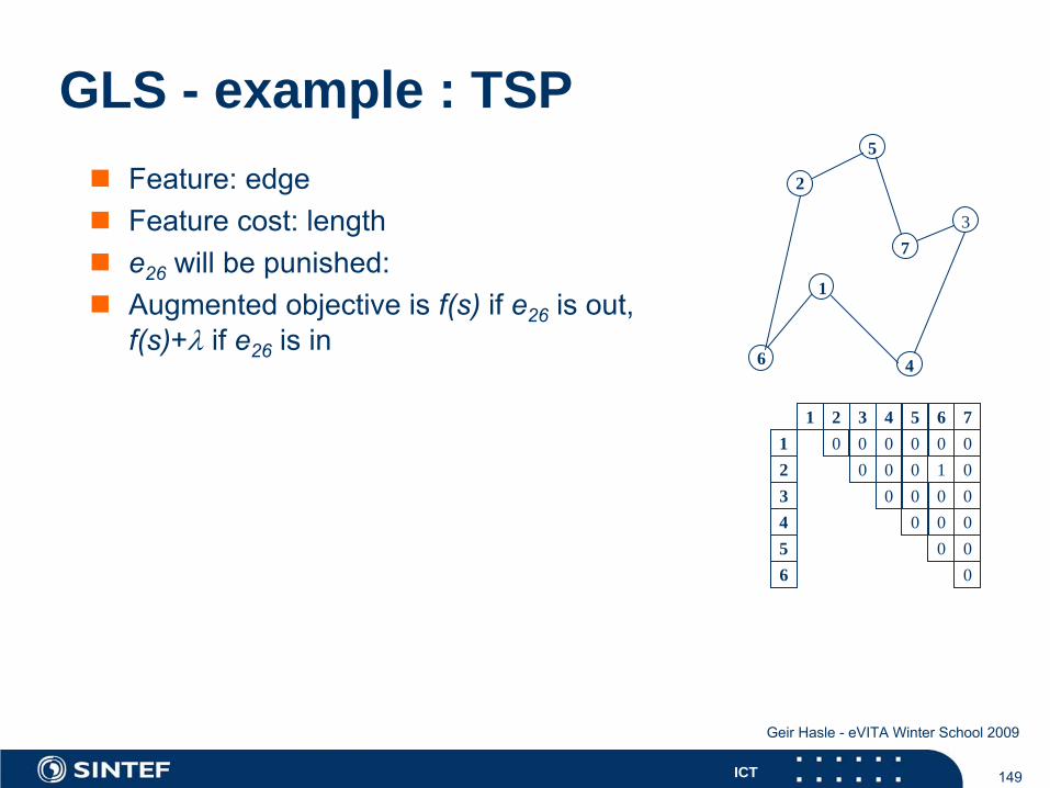
GLS - example : TSPFeature: edgeFeature cost: lengthe26 will be punished:Augmented objective is f(s) if e26 is out, f(s)+λ if e26 is in
4
1
6
5
7
2
3
1 2 3 4 5 6 71 0 0 02 0 0 03 0 0 0
0 0
0
001
4 0 05 0 06 0
0
150ICT
Geir Hasle - eVITA Winter School 2009
GLS - example : TSP
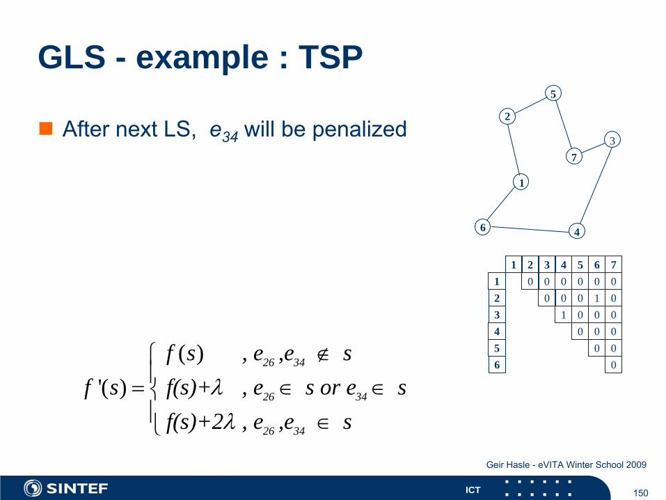
After next LS, e34 will be penalized
1 2 3 4 5 6 71 0 0 02 0 0 03 1 0 0
0 0
0
001
4 0 05 0 06 0
0
4
1
6
5
7
2
3
( )'( )
∉⎧⎪= ∈ ∈⎨⎪ ∈⎩
26 34
26 34
26 34
f s , e ,e sf s f(s)+ , e s or e s
f(s)+2 , e ,e s λλ
151ICT
Geir Hasle - eVITA Winter School 2009
GLS vs. SA
SA Local optima avoided by uphill movesLooping avoided by randomnessHigh temperatures give bad solutionsLow temperatures: convergence to local minimumThe cooling schedule is critical and problem dependent
GLS visits local minima, but will escapeNo uphill moves, but changes landscapeDeterministic (but probabilistic elements are easily added)
152ICT
Geir Hasle - eVITA Winter School 2009
GLS vs. Tabu SearchSimilarities ...Some arguments, from the GLS community ...TS utilizes frequency based (long term) memory used to penalizefeatures that are often present (for diversification)GLS utilizes memory (pi) throughout the search, not in phasesGLS penalizes on the basis of both cost and frequencyTS penalizes only on the basis of frequency, may avoid “good”featuresGLS avoids this by utilizing domain knowledge (ci) In GLS the probability for a feature to be penalized is reducedaccording to the number of times it has been penalized beforeui(smin , ei ) = Ii* ci /(1+pi )
153ICT
Geir Hasle - eVITA Winter School 2009
Fast Local SearchHeuristic limitation of neighborhoods (a la Candidate Lists)Idea
partition of neighborhood into sub-neighborhoodsStatus sub-neighborhoods: active or non-activeOnly search in active sub-neighborhoodsAssociation of properties to sub-neighborhoods
property ⇔ neighborhood that change status of this property
General idea, particularly well suited for GLS
154ICT
Geir Hasle - eVITA Winter School 2009
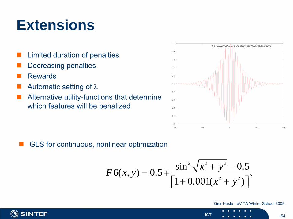
GLS for continuous, nonlinear optimization
Extensions
Limited duration of penaltiesDecreasing penaltiesRewardsAutomatic setting of λAlternative utility-functions that determinewhich features will be penalized
2 2 2
22 2
sin 0.56( , ) 0.51 0.001( )
x yF x yx y+ −
= ++ +⎡ ⎤⎣ ⎦
0
0.1
0.2
0.3
0.4
0.5
0.6
0.7
0.8
0.9
1
-100 -50 0 50 100
0.5+( sin(sqrt(x*x))*sin(sqrt(x*x)) -0.5)/((1+0.001*(x*x)) * (1+0.001*(x*x)))
155ICT
Geir Hasle - eVITA Winter School 2009
Genetic Algorithms (GA)
Rechenberg, Schwefel 1960-1970Holland et al. 1970iesFunction optimizationAI (games, pattern matching, ...)ORBasic idea
intelligent exploration of search spaces based on randomnessparallelismanalogies from evolutionary biology
156ICT
Geir Hasle - eVITA Winter School 2009
GA – Analogies with biology
Representation of complex objectsby vector of simple elementsChromosomesSelective breedingDarwinistic evolution
Classical GA for DOP: Binary encoding
157ICT
Geir Hasle - eVITA Winter School 2009
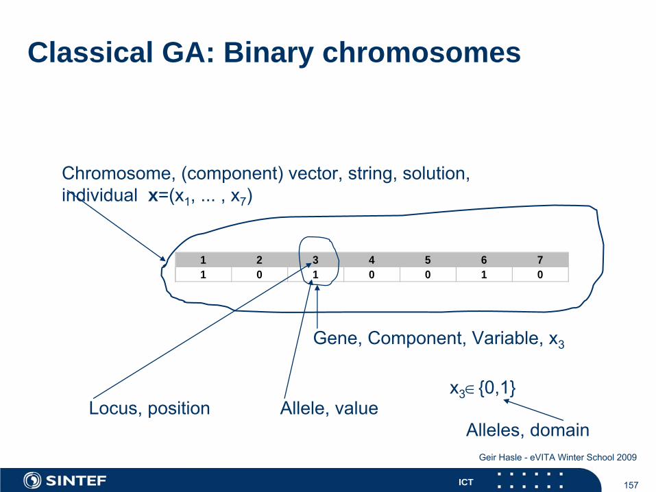
Classical GA: Binary chromosomes
1 2 3 4 5 6 71 0 1 0 0 1 0
Chromosome, (component) vector, string, solution, individual x=(x1
, ... , x7
)
Gene, Component, Variable, x3
Locus, position Allele, valuex3
∈{0,1}
Alleles, domain
158ICT
Geir Hasle - eVITA Winter School 2009
Genotype, Phenotype, Population
Genotypechromosomecollection of chromosomescoded string, collection of coded strings
Phenotypethe physical expressionattributes of a (collection of) solutions
Population – a set of solutions
159ICT
Geir Hasle - eVITA Winter School 2009
Genetic operators
Manipulate chromosomes/solutionsMutation: Unary operatorCrossover: Binary (or n-ary) operatorInversion...
160ICT
Geir Hasle - eVITA Winter School 2009
Assessment of individuals
”Fitness”Related to objective for DOPMaximizedUsed in selection (”Survival of the fittest”)Fitness is normally normalized
[ ]f : → 0,1S
161ICT
Geir Hasle - eVITA Winter School 2009
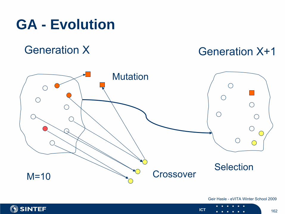
GA - Evolution
N generations of populationsFor each generation (step in evolution)
selection of individuals for genetic operatorsformation of new individualsselection of individuals that will survive
Population size (typically fixed) M
162ICT
Geir Hasle - eVITA Winter School 2009
GA - EvolutionGeneration
X Generation
X+1
Crossover
Mutation
SelectionM=10
163ICT
Geir Hasle - eVITA Winter School 2009
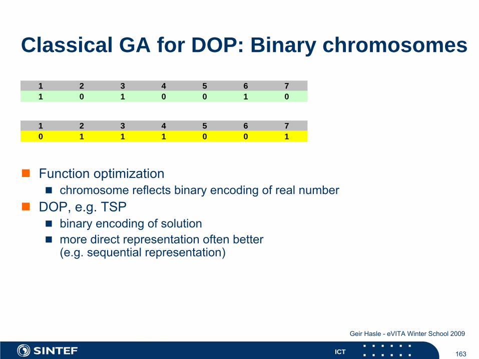
Classical GA for DOP: Binary chromosomes
Function optimizationchromosome reflects binary encoding of real number
DOP, e.g. TSPbinary encoding of solution more direct representation often better (e.g. sequential representation)
1 2 3 4 5 6 71 0 1 0 0 1 0
1 2 3 4 5 6 70 1 1 1 0 0 1
164ICT
Geir Hasle - eVITA Winter School 2009
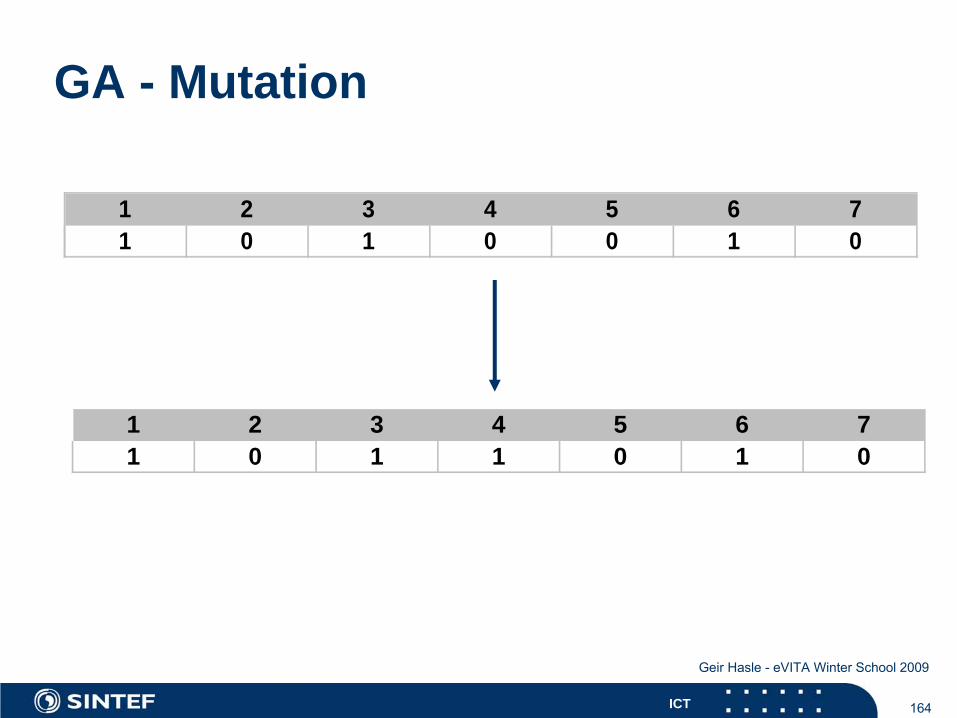
GA - Mutation
1 2 3 4 5 6 71 0 1 0 0 1 0
1 2 3 4 5 6 71 0 1 1 0 1 0
165ICT
Geir Hasle - eVITA Winter School 2009
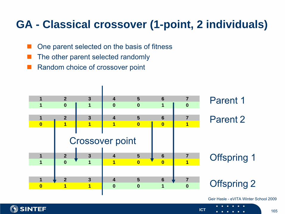
1 2 3 4 5 6 70 1 1 0 0 1 0 Offspring
2
1 2 3 4 5 6 71 0 1 1 0 0 1 Offspring
1
GA - Classical crossover (1-point, 2 individuals)
One parent selected on the basis of fitnessThe other parent selected randomlyRandom choice of crossover point
1 2 3 4 5 6 71 0 1 0 0 1 0 Parent
1
1 2 3 4 5 6 70 1 1 1 0 0 1 Parent
2
Crossover
point
166ICT
Geir Hasle - eVITA Winter School 2009
GA - Classical crossover cont’d.
Random individual in population exchanged for one of theoffspringReproduction as long as you have energySequence of almost equal populationsMore elitist alternative
the most fit individual selected as one parentcrossover until M offspring have been bornchange the whole population
Lots of other alternatives ...Basic GA with classical crossover and mutation often works well
167ICT
Geir Hasle - eVITA Winter School 2009
GA – standard reproduction plan
Fixed polulation sizeStandard 1-point 2-individual crossoverMutation
standard: offspring are mutateda certain (small) probability that a certain gene is mutated
168ICT
Geir Hasle - eVITA Winter School 2009
Theoretical analysis of GA (Holland)
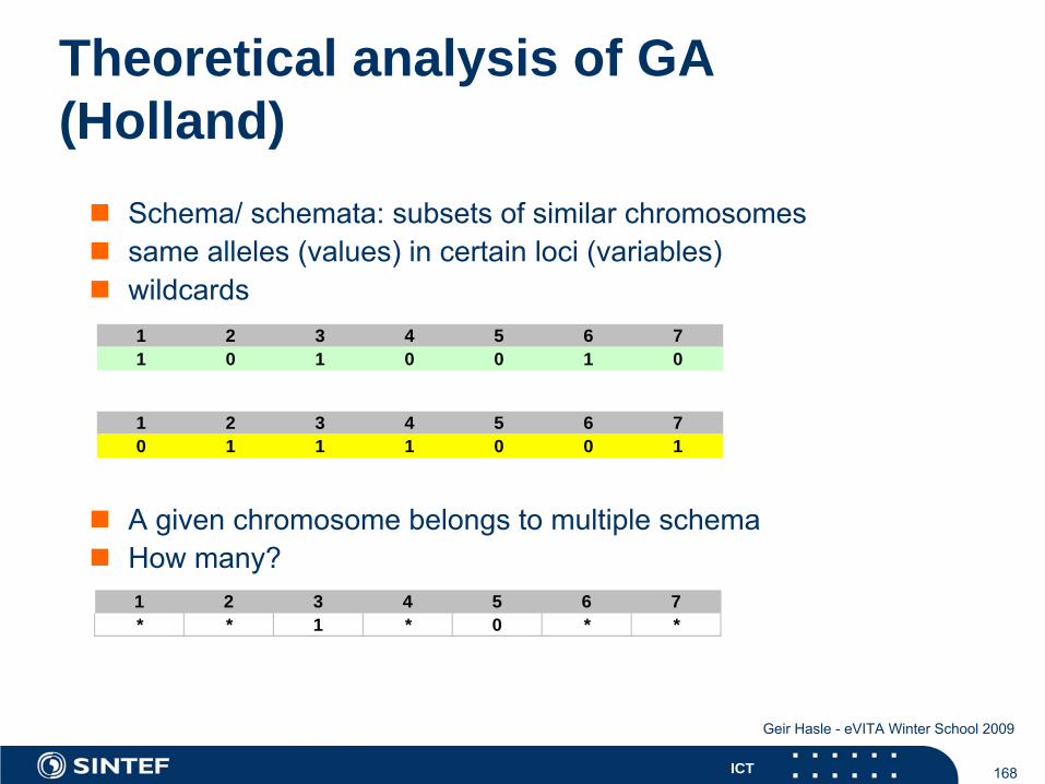
Schema/ schemata: subsets of similar chromosomessame alleles (values) in certain loci (variables)wildcards
A given chromosome belongs to multiple schemaHow many?
1 2 3 4 5 6 71 0 1 0 0 1 0
1 2 3 4 5 6 70 1 1 1 0 0 1
1 2 3 4 5 6 7* * 1 * 0 * *
169ICT
Geir Hasle - eVITA Winter School 2009
Schema - fitness
Every time we evaluate fitness to a chromosome, information onaverage fitness to each of the associated schemata is gatheredA populasjon may contain M 2n schemataIn practice: overlap
170ICT
Geir Hasle - eVITA Winter School 2009
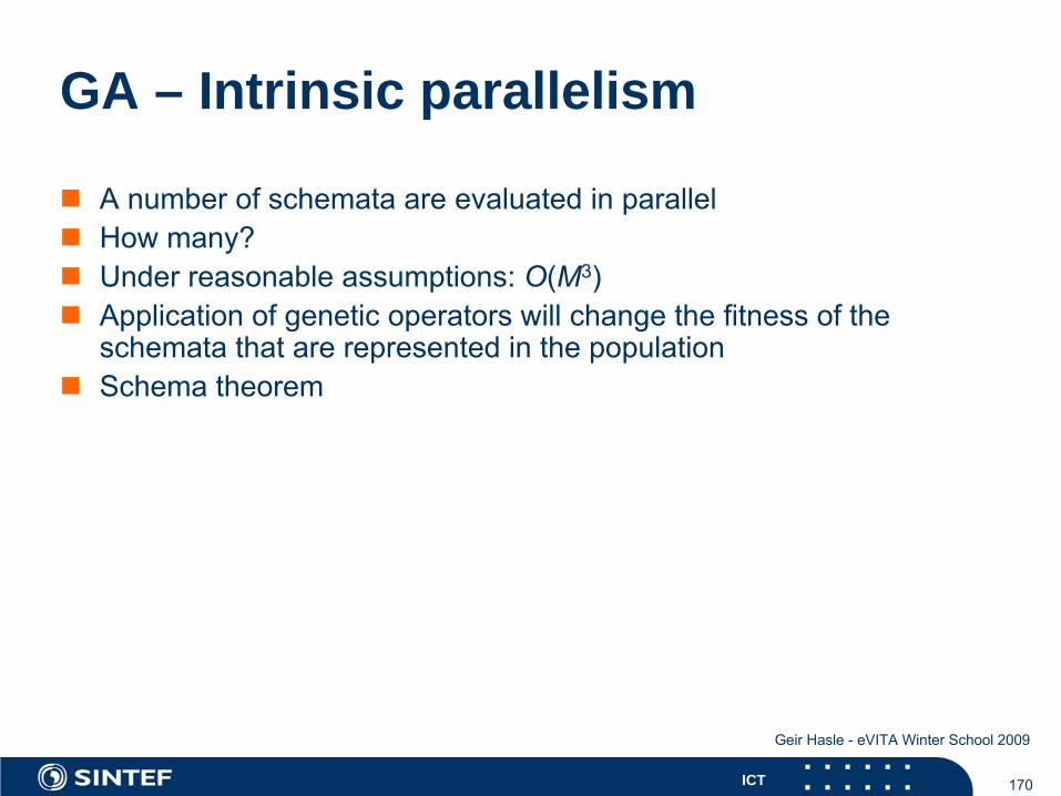
GA – Intrinsic parallelism
A number of schemata are evaluated in parallelHow many?Under reasonable assumptions: O(M3)Application of genetic operators will change the fitness of theschemata that are represented in the populationSchema theorem
171ICT
Geir Hasle - eVITA Winter School 2009
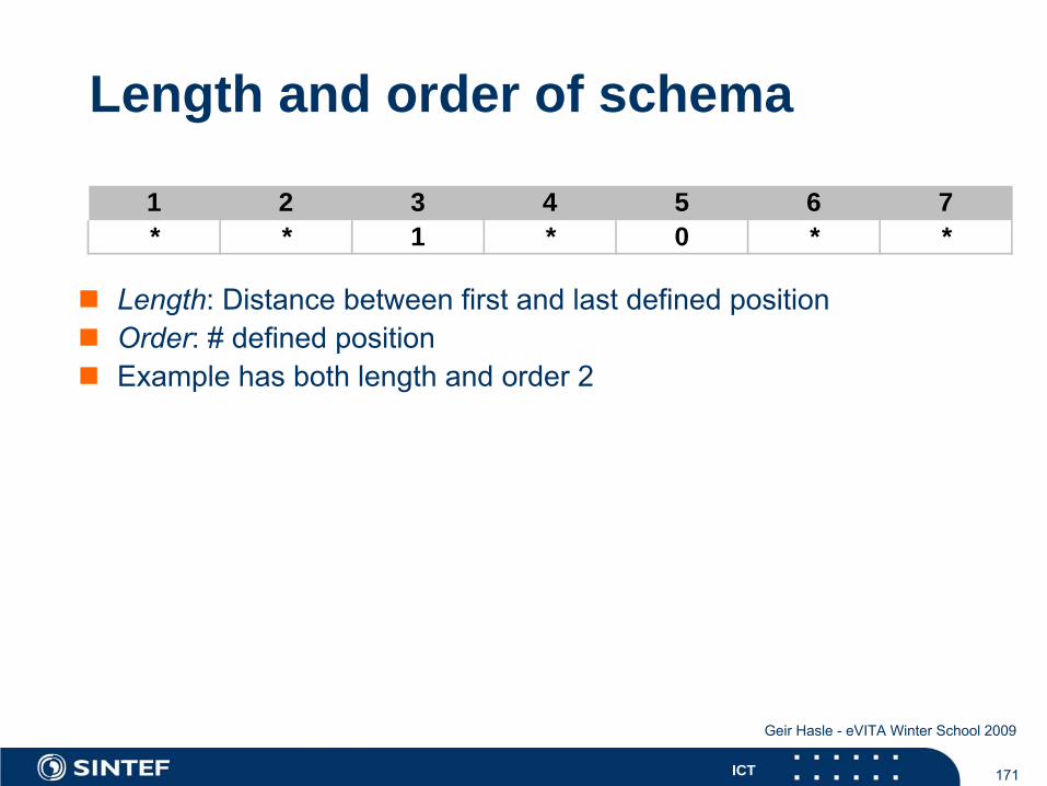
Length and order of schema
Length: Distance between first and last defined positionOrder: # defined positionExample has both length and order 2
1 2 3 4 5 6 7* * 1 * 0 * *
172ICT
Geir Hasle - eVITA Winter School 2009
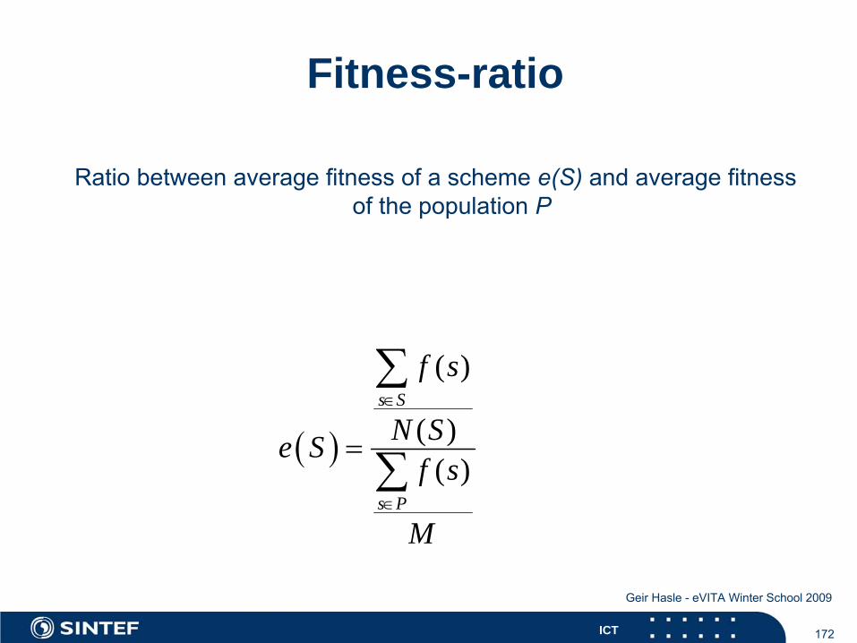
Fitness-ratio
Ratio between
average
fitness
of
a scheme
e(S)
and average
fitness of
the
population
P
( )
( )
( )( )
s S
s P
f s
N Se Sf s
M
∈
∈
=
∑
∑
173ICT
Geir Hasle - eVITA Winter School 2009
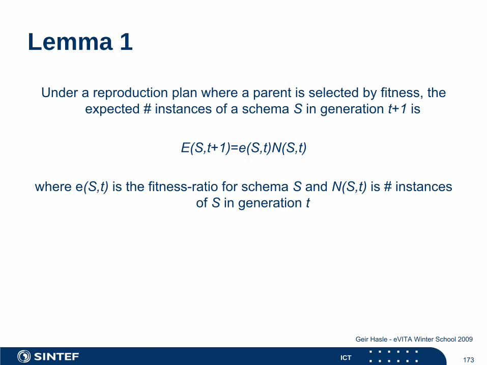
Lemma 1
Under a reproduction
plan where
a parent
is selected
by fitness, the expected
# instances
of
a schema
S
in generation
t+1 is
E(S,t+1)=e(S,t)N(S,t)
where
e(S,t)
is the
fitness-ratio
for schema
S
and N(S,t)
is # instances of
S
in generation
t
174ICT
Geir Hasle - eVITA Winter School 2009
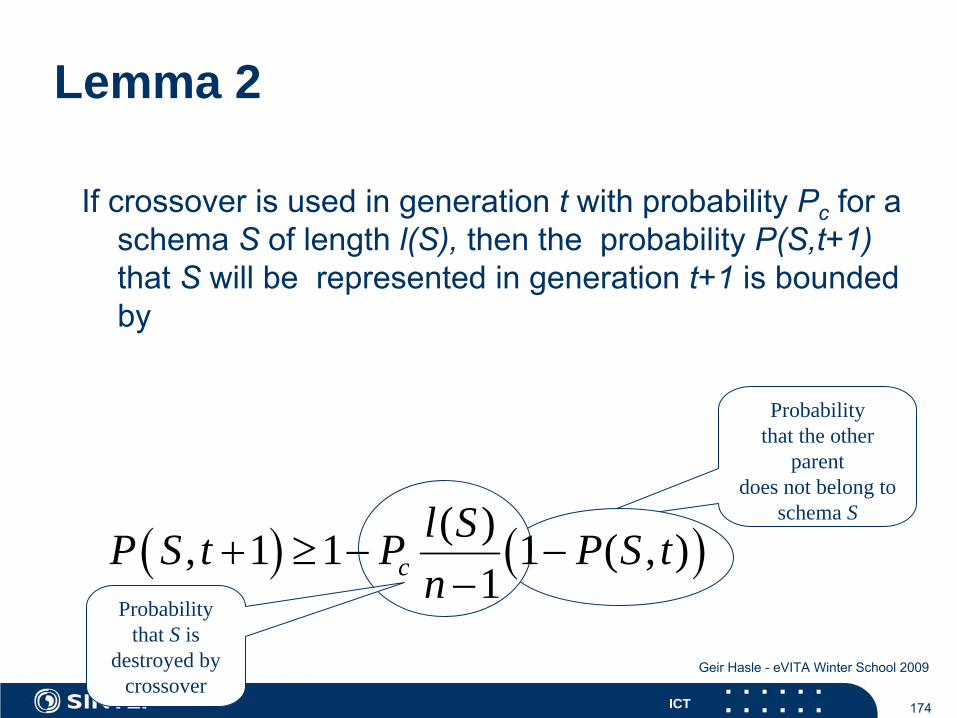
Probabilitythat the other
parentdoes not belong to
schema S
Probabilitythat S is
destroyed by crossover
Lemma 2
If
crossover
is used in generation
t
with
probability
Pc
for a schema
S
of
length
l(S), then
the
probability
P(S,t+1)
that
S
will
be represented
in generation
t+1
is bounded by
( ) ( )( ), 1 1 1 ( , )1c
l SP S t P P S tn
+ ≥ − −−
175ICT
Geir Hasle - eVITA Winter School 2009
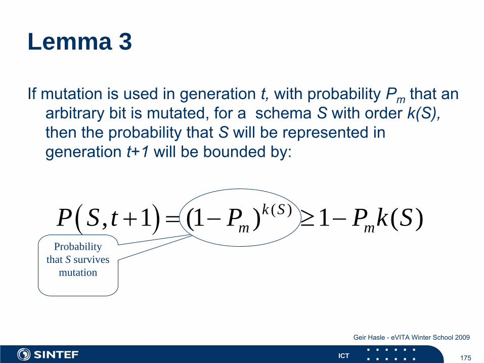
Probabilitythat S survives
mutation
Lemma 3
If
mutation
is used in generation
t,
with
probability
Pm
that
an arbitrary
bit is mutated, for a schema
S
with
order k(S),
then
the
probability
that
S
will
be represented
in generation
t+1
will
be bounded
by:
( ) ( ), 1 (1 ) 1 ( )k Sm mP S t P P k S+ = − ≥ −
176ICT
Geir Hasle - eVITA Winter School 2009
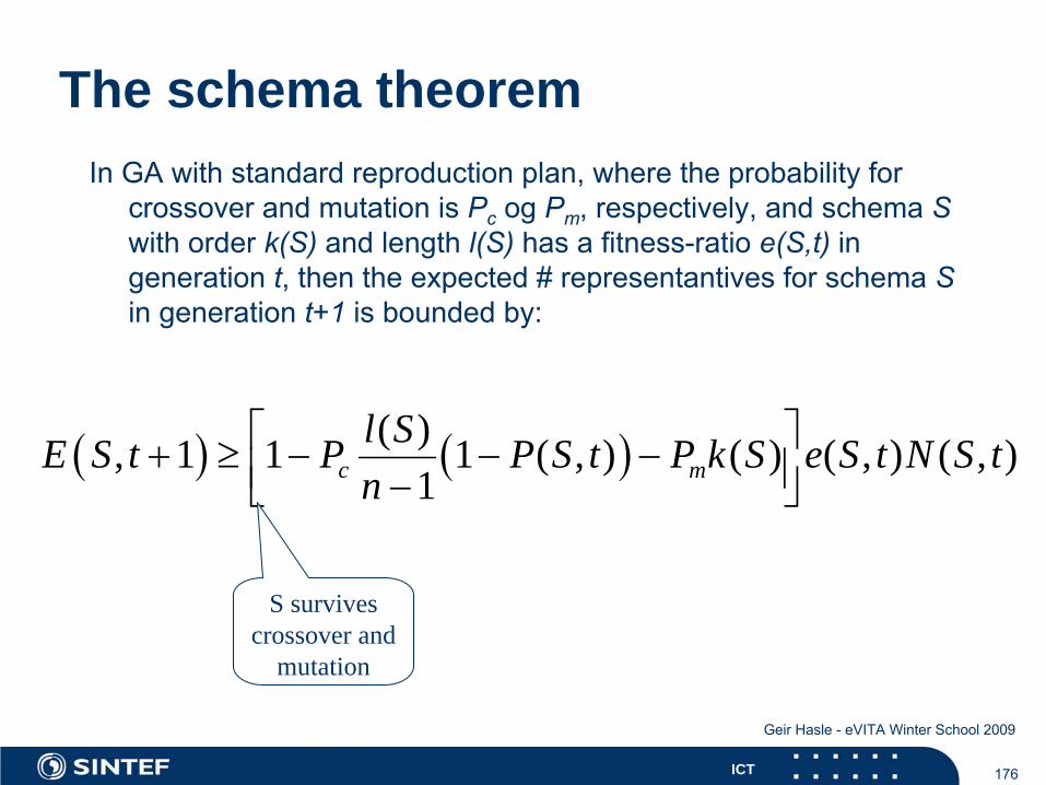
The schema theoremIn GA with
standard reproduction
plan, where
the
probability
for
crossover
and mutation
is Pc
og Pm
, respectively, and schema
S with
order k(S)
and length
l(S)
has a fitness-ratio
e(S,t)
in
generation
t, then
the
expected
# representantives
for schema
S in generation
t+1
is bounded
by:
( ) ( )( ), 1 1 1 ( , ) ( ) ( , ) ( , )1c m
l SE S t P P S t P k S e S t N S tn
⎡ ⎤+ ≥ − − −⎢ ⎥−⎣ ⎦
S survives crossover and
mutation
177ICT
Geir Hasle - eVITA Winter School 2009
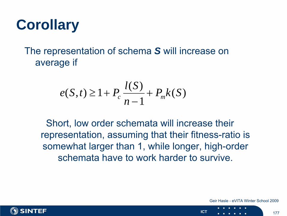
CorollaryThe
representation
of
schema
S will
increase
on
average
if
( )( , ) 1 ( )1c m
l Se S t P P k Sn
≥ + +−
Short, low
order schemata
will
increase
their representation, assuming
that
their
fitness-ratio
is
somewhat
larger
than
1, while
longer, high-order schemata
have to work
harder
to survive.

178ICT
Geir Hasle - eVITA Winter School 2009
GA – Building block hypothesis
Goldberg (1989)Short, low order schemata are combined to increasinglybetter solutions
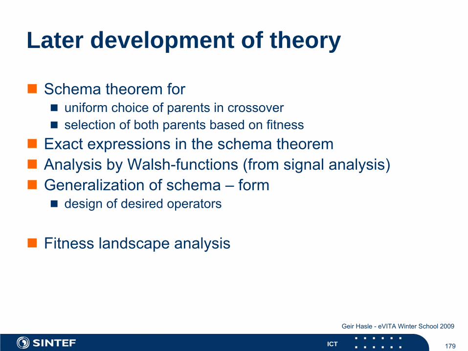
179ICT
Geir Hasle - eVITA Winter School 2009
Later development of theory
Schema theorem foruniform choice of parents in crossoverselection of both parents based on fitness
Exact expressions in the schema theoremAnalysis by Walsh-functions (from signal analysis)Generalization of schema – form
design of desired operators
Fitness landscape analysis
180ICT
Geir Hasle - eVITA Winter School 2009
GA – Observations, Extensions, and Modifications
many knobs to turna lot of literature, chaoticsomewhat unclear terminologymodifications
populationencodingoperatorshybridizationparallelization
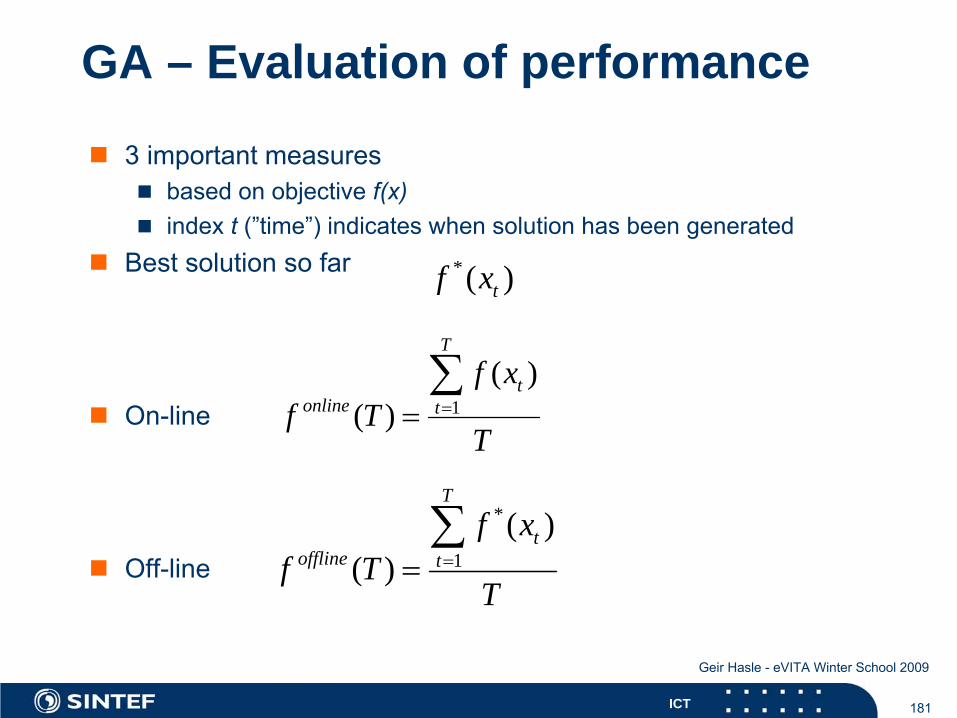
181ICT
Geir Hasle - eVITA Winter School 2009
GA – Evaluation of performance
3 important measuresbased on objective f(x)index t (”time”) indicates when solution has been generated
Best solution so far
On-line
Off-line
*( )tf x
1( )
( )
T
tonline t
f xf T
T==∑
*
1( )
( )
T
toffline t
f xf T
T==∑
182ICT
Geir Hasle - eVITA Winter School 2009
GA – Population size
Small populations – low coverageLarge populations – computationally demandingOptimal size increases exponentially with string length in binary encodingsRule of thumb: 30between n and 2n (Alander)
183ICT
Geir Hasle - eVITA Winter School 2009
GA – Initial population
normal: random solutionsalternative: ”seeds”: high quality solutions
quicker convergencepremature convergence
184ICT
Geir Hasle - eVITA Winter School 2009
GA – Selection mechanisms
Generation gap/overlap vs total exchange of populationIncremental selection works well in many applications
Alternative setupA part of the population is selected for reproductionOffspring replace randomly selected individualsMay work better
Duplication of solution should be avoidedThe incumbent should surviveElitisme/Selective death
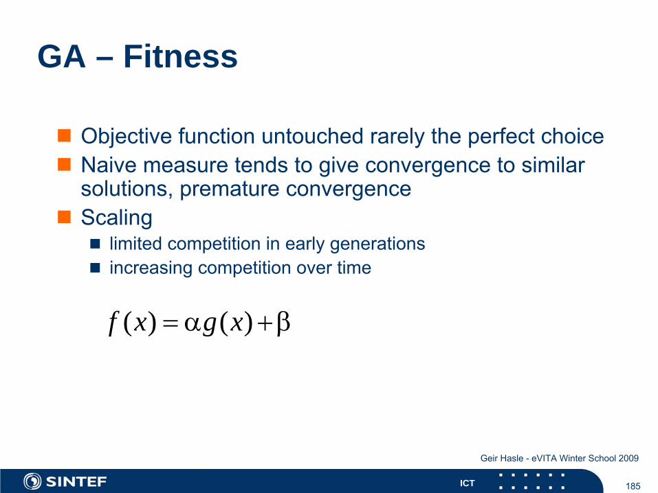
185ICT
Geir Hasle - eVITA Winter School 2009
GA – Fitness
Objective function untouched rarely the perfect choiceNaive measure tends to give convergence to similarsolutions, premature convergenceScaling
limited competition in early generationsincreasing competition over time
( ) ( )f x g x= α +β
186ICT
Geir Hasle - eVITA Winter School 2009
GA – Fitness/Selection
Use ranks rather than objectiveTournament selection
random selection of groupsthe most fit in each group are selected
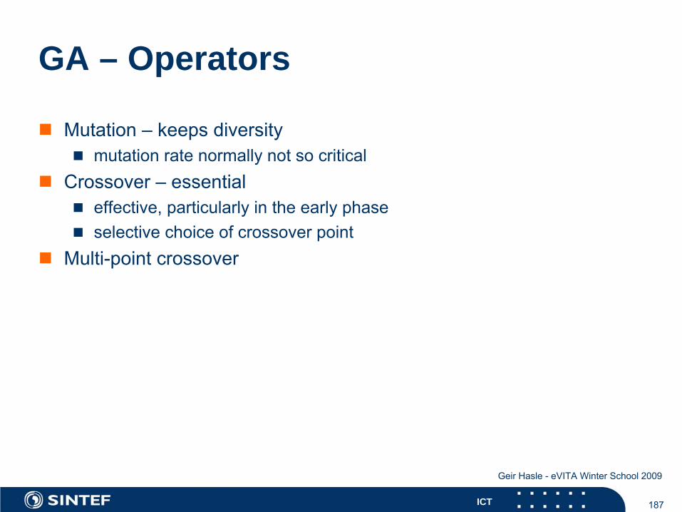
187ICT
Geir Hasle - eVITA Winter School 2009
GA – Operators
Mutation – keeps diversitymutation rate normally not so critical
Crossover – essentialeffective, particularly in the early phaseselective choice of crossover point
Multi-point crossover
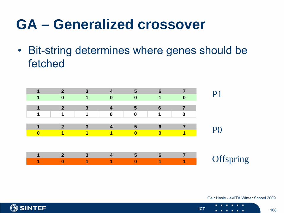
188ICT
Geir Hasle - eVITA Winter School 2009
GA – Generalized crossover
1 2 3 4 5 6 71 1 1 0 0 1 0
•
Bit-string
determines
where
genes
should
be fetched
1 2 3 4 5 6 71 0 1 0 0 1 0
1 2 3 4 5 6 70 1 1 1 0 0 1
1 2 3 4 5 6 71 0 1 1 0 1 1
P1
P0
Offspring
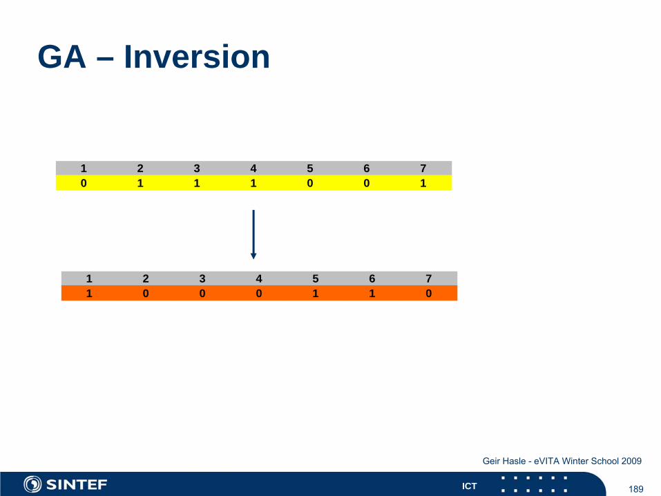
189ICT
Geir Hasle - eVITA Winter School 2009
GA – Inversion
1 2 3 4 5 6 70 1 1 1 0 0 1
1 2 3 4 5 6 71 0 0 0 1 1 0
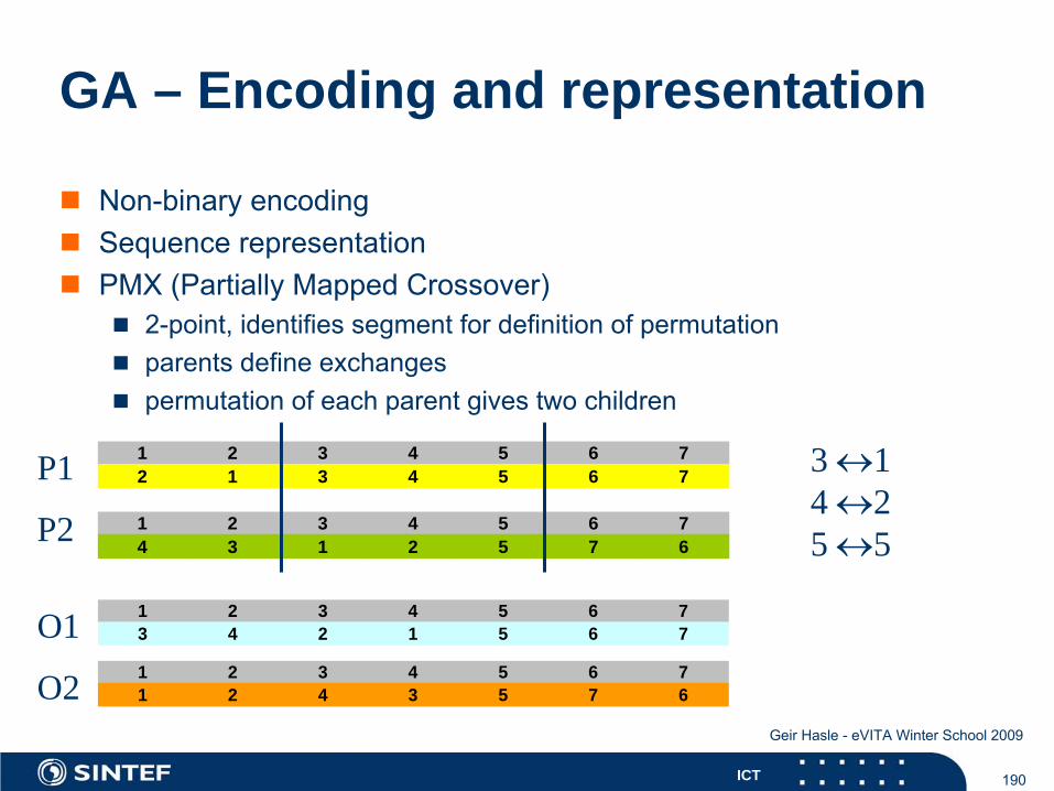
190ICT
Geir Hasle - eVITA Winter School 2009
GA – Encoding and representation
Non-binary encodingSequence representationPMX (Partially Mapped Crossover)
2-point, identifies segment for definition of permutationparents define exchangespermutation of each parent gives two children
1 2 3 4 5 6 72 1 3 4 5 6 7
1 2 3 4 5 6 74 3 1 2 5 7 6
1 2 3 4 5 6 73 4 2 1 5 6 7
3 ↔14 ↔25 ↔5
1 2 3 4 5 6 71 2 4 3 5 7 6
P1
P2
O1
O2
191ICT
Geir Hasle - eVITA Winter School 2009
GA - Hybridization
Strength and weakness of GA: domain independenceConstraints may be a challenge - penaltiesHybridization
Seeding, good individuals in initial population”Local search” on individualsCombination with other metaheuristics
192ICT
Geir Hasle - eVITA Winter School 2009
GA - parallelization
Fitness-evaluationFine grained parallelization
every solution its own process(a)synchronous parallelization
Coarse grained parallelizationsub-populationsthe island model
193ICT
Geir Hasle - eVITA Winter School 2009
GA - Summary
Inspired by biological evolutionPopulation of solutions that evolvesGenetic operatorsRandomnessDomain independence – encodingLacks utilization of problem structureIntrinsic parallelism – schema, vocabulariesRobust, but danger of premature convergenceGood diversification, lacks somewhat in intensificationHybrid with local search: Memetic algorithms
194ICT
Geir Hasle - eVITA Winter School 2009
Memetic - meme
Introduced by Richard Dawkins (1976): ”The Selfish Gene”Analogous to gene, in cultural evolution
”Examples
of
memes are
tunes, ideas, catch-phrases, clothes
fashions, ways
of
making pots or building
arches.”
195ICT
Geir Hasle - eVITA Winter School 2009
Trends GA –> Evolutionary Algorithms
More direct representation of solutionmore natural encoding of solutionsspecialized crossover- and mutation operators
More intensificationlocal search (”special mutation operators”) to local optimumhybridization of e.g. SA or TA to get deeperMemetic algorithms
Parallel computing
1-population, no crossover EA ...
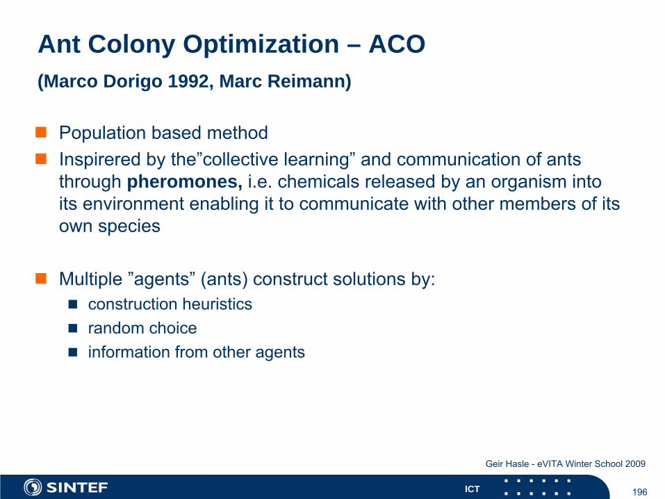
196ICT
Geir Hasle - eVITA Winter School 2009
Ant Colony Optimization – ACO (Marco Dorigo 1992, Marc Reimann)
Population based methodInspirered by the”collective learning” and communication of ants through pheromones, i.e. chemicals released by an organism intoits environment enabling it to communicate with other members of itsown species
Multiple ”agents” (ants) construct solutions by:construction heuristicsrandom choiceinformation from other agents
197ICT
Geir Hasle - eVITA Winter School 2009
Ants (cont´d.)Social insectsSelf organizing collective behaviorComplex dynamics emerges from simple individuals
„emergent behaviour“„swarm intelligence“
Interesting social phenomena (Work sharing, Allocation of tasks, Organization of „graveyards“)Transport management, finding food (e.g. Lasius niger)
198ICT
Geir Hasle - eVITA Winter School 2009
Ants and paths
Formation and following of paths by simple, local rulesEvery ant legger lays a pheromone trail from nest to food source and backPheromone evaporatesAnts follow pheromone trails of other ants, according to intensityStrong paths get stronger, weak paths get weakerPositive feedback, reinforcement learning
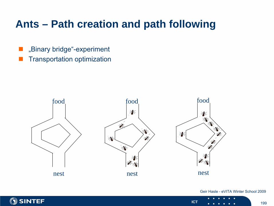
199ICT
Geir Hasle - eVITA Winter School 2009
Ants – Path creation and path following
„Binary bridge“-experimentTransportation optimization
nest
food
nest
food
nest
food
200ICT
Geir Hasle - eVITA Winter School 2009
Ant Colony Optimization (ACO) for DOP
Introduced by Dorigo, Maniezzo & Colorni 1992Population based metaheuristicEvery „ant“ in the population constructs a solutionWhen they all are finished, a memory (artificialpheromone) is updatedConstruction and memory update is repeated until stopcriterion is satisfied
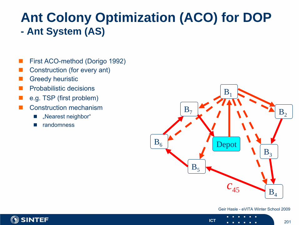
201ICT
Geir Hasle - eVITA Winter School 2009
Ant Colony Optimization (ACO) for DOP - Ant System (AS)
First ACO-method (Dorigo 1992)Construction (for every ant)Greedy heuristicProbabilistic decisionse.g. TSP (first problem)Construction mechanism
„Nearest neighbor“randomness
Depot
B1
B2
B6B3
B4
B5
B7
45c
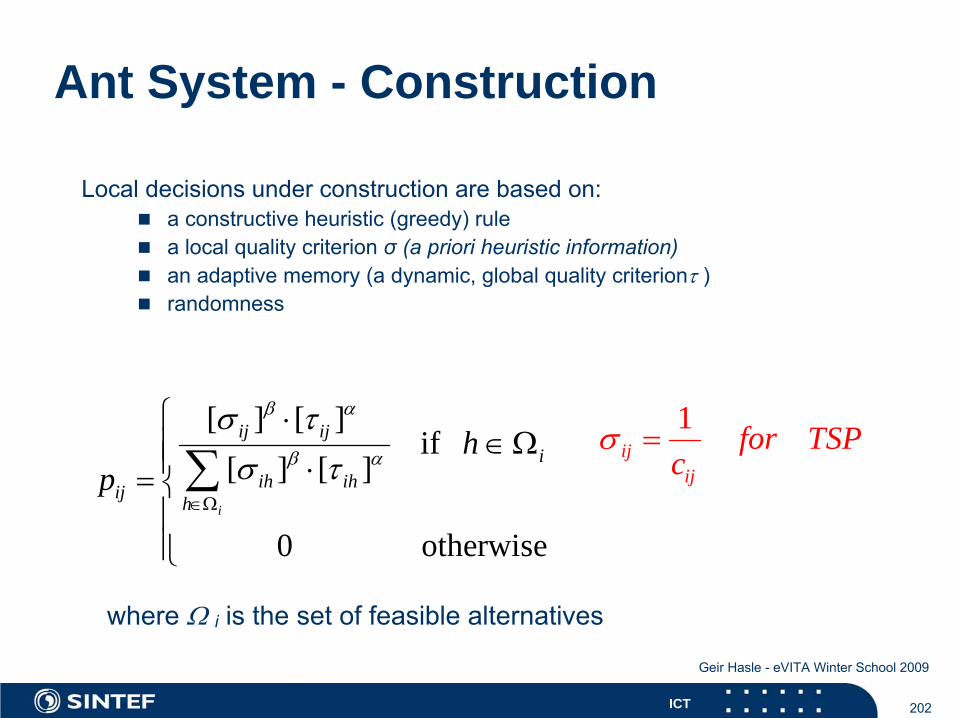
202ICT
Geir Hasle - eVITA Winter School 2009
Ant System - Construction
Local
decisions
under
construction
are
based
on:a constructive heuristic (greedy) rulea local quality criterion σ (a priori heuristic information)an adaptive memory (a dynamic, global quality criterionτ )randomness
[ ] [ ]if
[ ] [ ]
0 otherwise∈Ω
⎧ ⋅∈Ω⎪⎪ ⋅= ⎨
⎪⎪⎩
∑i
ij iji
ih ihij h
hp
β α
β α
σ τσ τ
where
Ω i
is
the
set
of feasible
alternatives
1ij
ij
for TSPc
σ =

203ICT
Geir Hasle - eVITA Winter School 2009
TSP-example: All edges
are
updated
for
each
iteration, for
each
ant
Ant System Update of dynamic informasjon (pheromone)
( )(1 ) , 0 1mij
m Mijij ρ τ ττ ρΔ
∈
= − ⋅ + < ≤∑
1 , if ( , )( )
0Δ
⎧ ∈⎪= ⎨⎪⎩
mmm
ij
i j sf s
otherwiseτ
mij
m MτΔ
∈∑
is
pheromone
on edge
(i,j) after
evaporation(1 ) ijρ τ− ⋅
is
the
added
pheromone
on edge
(i,j)
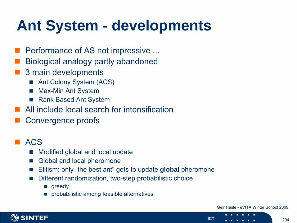
204ICT
Geir Hasle - eVITA Winter School 2009
Ant System - developmentsPerformance of AS not impressive ...Biological analogy partly abandoned3 main developments
Ant Colony System (ACS)Max-Min Ant SystemRank Based Ant System
All include local search for intensificationConvergence proofs
ACSModified global and local updateGlobal and local pheromoneElitism: only „the best ant“ gets to update global pheromoneDifferent randomization, two-step probabilistic choice
greedyprobabilistic among feasible alternatives
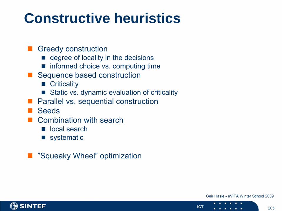
205ICT
Geir Hasle - eVITA Winter School 2009
Constructive heuristics
Greedy constructiondegree of locality in the decisionsinformed choice vs. computing time
Sequence based constructionCriticalityStatic vs. dynamic evaluation of criticality
Parallel vs. sequential constructionSeedsCombination with search
local searchsystematic
”Squeaky Wheel” optimization
206ICT
Geir Hasle - eVITA Winter School 2009
Simple remedy to continue from local optima
Restart from a new solutionMulti-start methods
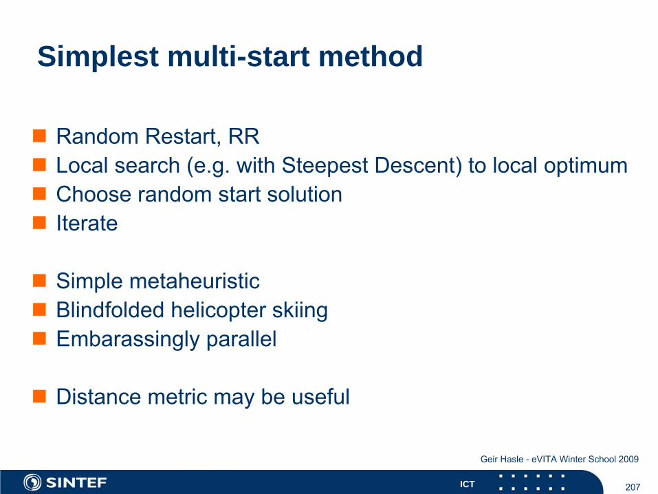
207ICT
Geir Hasle - eVITA Winter School 2009
Simplest multi-start method
Random Restart, RRLocal search (e.g. with Steepest Descent) to local optimumChoose random start solutionIterate
Simple metaheuristicBlindfolded helicopter skiingEmbarassingly parallel
Distance metric may be useful
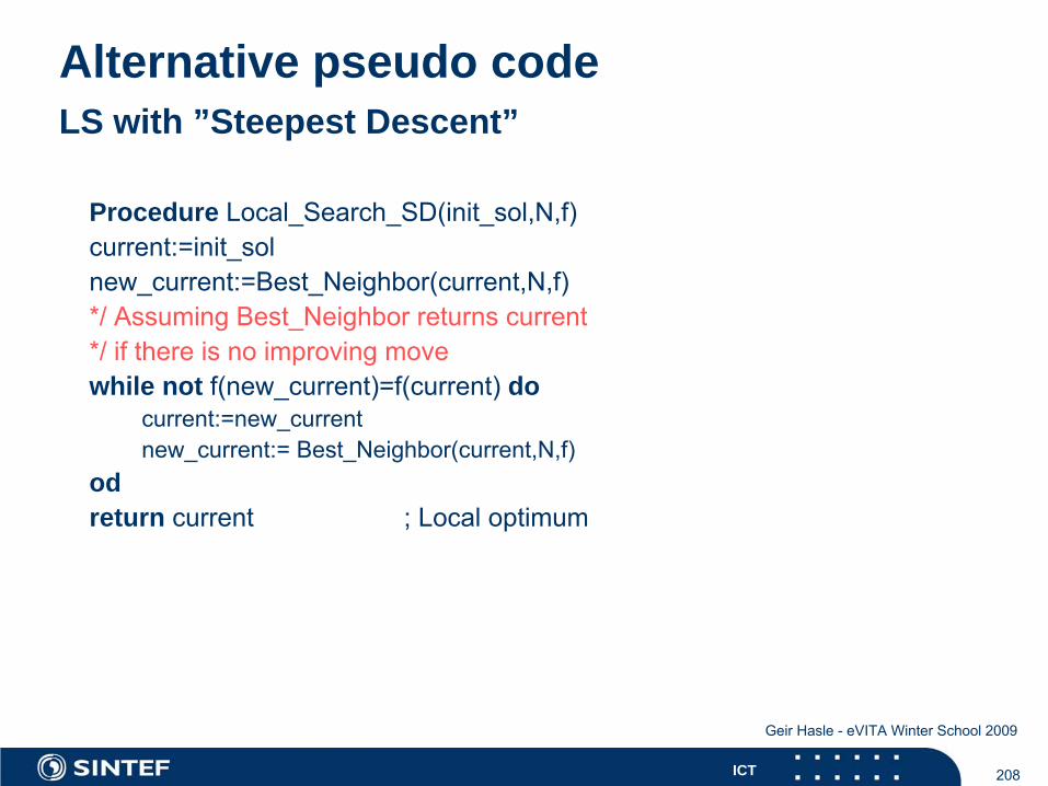
208ICT
Geir Hasle - eVITA Winter School 2009
Alternative pseudo code LS with ”Steepest Descent”
Procedure Local_Search_SD(init_sol,N,f)current:=init_solnew_current:=Best_Neighbor(current,N,f)*/ Assuming
Best_Neighbor
returns
current
*/ if
there
is no
improving
movewhile not f(new_current)=f(current) do
current:=new_currentnew_current:= Best_Neighbor(current,N,f)
odreturn current
; Local
optimum
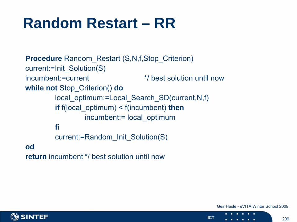
209ICT
Geir Hasle - eVITA Winter School 2009
Random Restart – RR
Procedure Random_Restart
(S,N,f,Stop_Criterion)current:=Init_Solution(S)incumbent:=current
*/ best solution
until
now
while not Stop_Criterion() dolocal_optimum:=Local_Search_SD(current,N,f)if f(local_optimum) < f(incumbent) then
incumbent:= local_optimumficurrent:=Random_Init_Solution(S)
odreturn incumbent
*/ best solution until now
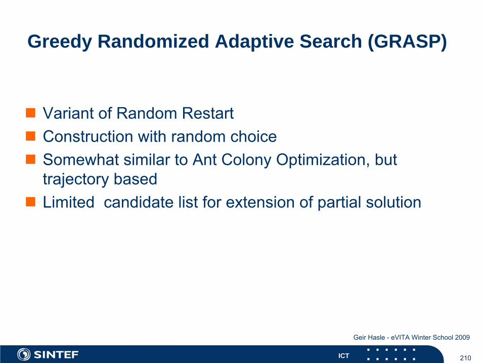
210ICT
Geir Hasle - eVITA Winter School 2009
Greedy Randomized Adaptive Search (GRASP)
Variant of Random RestartConstruction with random choiceSomewhat similar to Ant Colony Optimization, but trajectory basedLimited candidate list for extension of partial solution
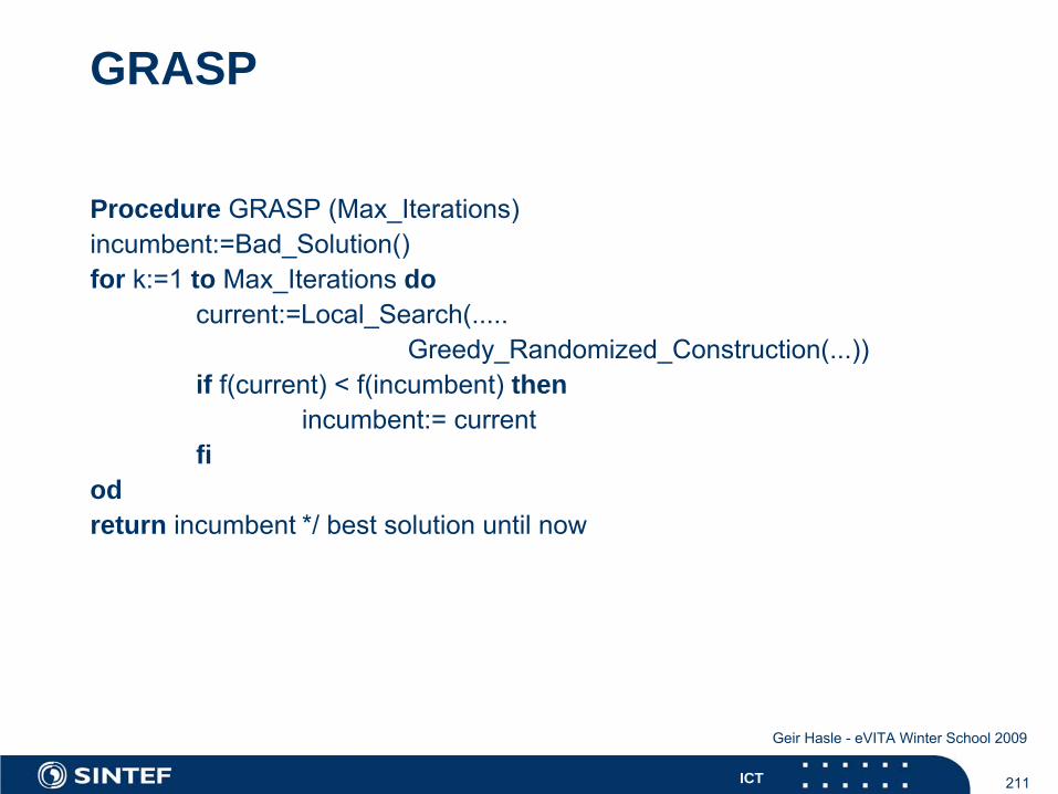
211ICT
Geir Hasle - eVITA Winter School 2009
GRASP
Procedure GRASP (Max_Iterations)incumbent:=Bad_Solution()for k:=1
to Max_Iterations
do
current:=Local_Search(.....Greedy_Randomized_Construction(...))
if f(current) < f(incumbent) thenincumbent:= current
fiodreturn incumbent
*/ best solution until now
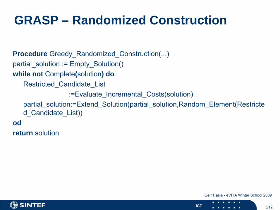
212ICT
Geir Hasle - eVITA Winter School 2009
GRASP – Randomized Construction
Procedure Greedy_Randomized_Construction(...)partial_solution
:= Empty_Solution()
while not Complete(solution) doRestricted_Candidate_List
:=Evaluate_Incremental_Costs(solution) partial_solution:=Extend_Solution(partial_solution,Random_Element(Restricte
d_Candidate_List))odreturn solution
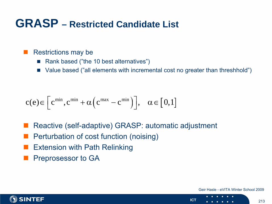
213ICT
Geir Hasle - eVITA Winter School 2009
GRASP – Restricted Candidate List
Restrictions may beRank based (”the 10 best alternatives”)Value based (”all elements with incremental cost no greater than threshhold”)
( ) [ ]min min max minc(e) c ,c c c , 0,1⎡ ⎤∈ + α − α∈⎣ ⎦
Reactive (self-adaptive) GRASP: automatic adjustmentPerturbation of cost function (noising)Extension with Path RelinkingPreprosessor to GA
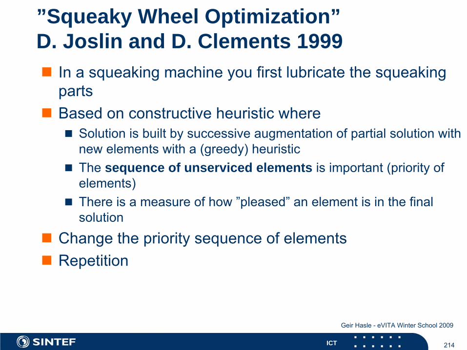
214ICT
Geir Hasle - eVITA Winter School 2009
”Squeaky Wheel Optimization” D. Joslin and D. Clements 1999
In a squeaking machine you first lubricate the squeakingpartsBased on constructive heuristic where
Solution is built by successive augmentation of partial solution withnew elements with a (greedy) heuristicThe sequence of unserviced elements is important (priority ofelements)There is a measure of how ”pleased” an element is in the final solution
Change the priority sequence of elementsRepetition

215ICT
Geir Hasle - eVITA Winter School 2009
Squeaky Wheel Optimization
Procedure Squeaky_Wheel_Optimization(f)Element_Priority_List
:=Determine_Element_Priorities() ; Static
prioritizationincumbent:=Some_Feasible_Solution()while not Stop_Criterion() do
solution:= Empty_Solution()while not Complete(solution) do
solution:=Augment_Solution(solution,Element_Priority_List)
odif f(solution)< f(incumbent) then incumbent:=solutionElement_Priority_List
:=Update_Element_Priorities(Element_Priority_List,solution)odreturn solution
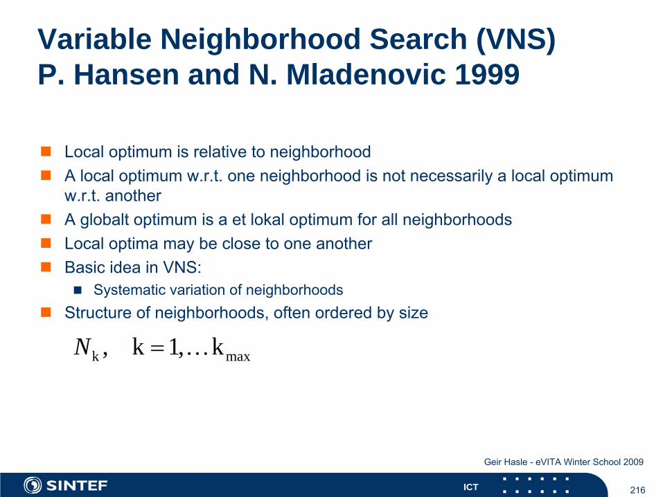
216ICT
Geir Hasle - eVITA Winter School 2009
Variable Neighborhood Search (VNS) P. Hansen and N. Mladenovic 1999
Local optimum is relative to neighborhoodA local optimum w.r.t. one neighborhood is not necessarily a local optimum w.r.t. anotherA globalt optimum is a et lokal optimum for all neighborhoodsLocal optima may be close to one anotherBasic idea in VNS:
Systematic variation of neighborhoodsStructure of neighborhoods, often ordered by size
k max, k 1, k= …N
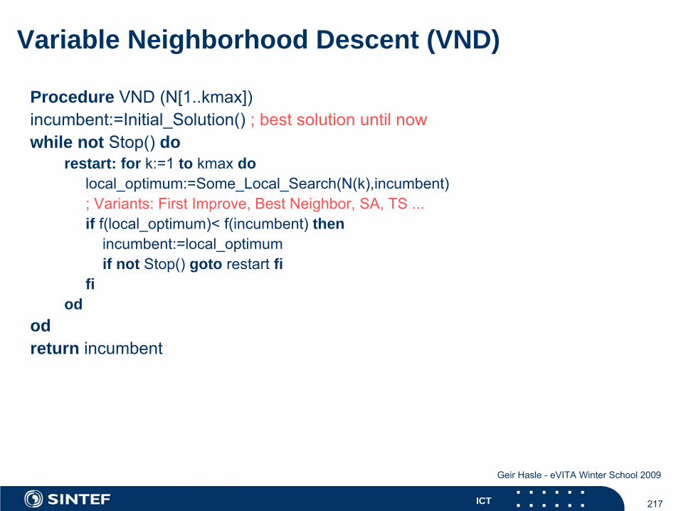
217ICT
Geir Hasle - eVITA Winter School 2009
Variable Neighborhood Descent (VND)
Procedure VND (N[1..kmax])incumbent:=Initial_Solution() ; best solution
until
now
while not Stop() dorestart: for k:=1
to kmax
dolocal_optimum:=Some_Local_Search(N(k),incumbent); Variants: First Improve, Best Neighbor, SA, TS ...if f(local_optimum)< f(incumbent) then
incumbent:=local_optimumif not Stop() goto restart
fifi
ododreturn incumbent
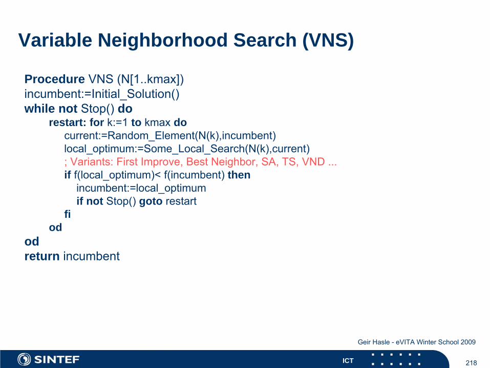
218ICT
Geir Hasle - eVITA Winter School 2009
Variable Neighborhood Search (VNS)
Procedure VNS (N[1..kmax])incumbent:=Initial_Solution()while not Stop() do
restart: for k:=1
to kmax
docurrent:=Random_Element(N(k),incumbent)local_optimum:=Some_Local_Search(N(k),current); Variants: First Improve, Best Neighbor, SA, TS, VND ...if f(local_optimum)< f(incumbent) then
incumbent:=local_optimumif not Stop() goto restart
fiod
odreturn incumbent
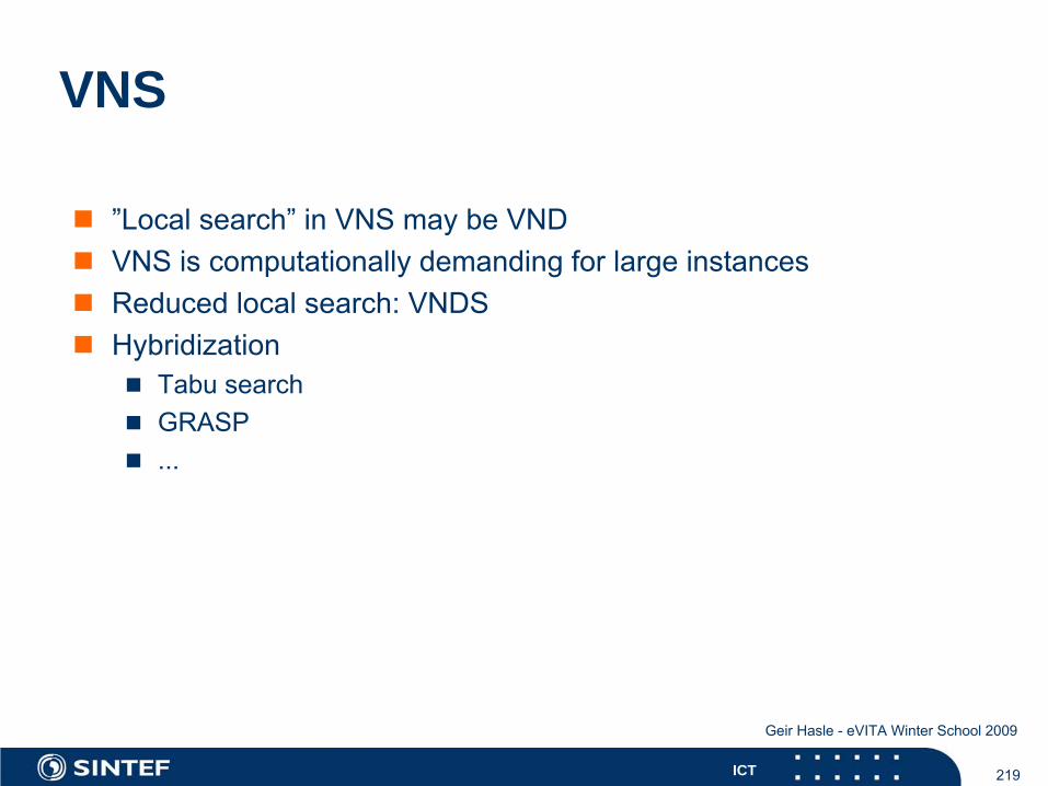
219ICT
Geir Hasle - eVITA Winter School 2009
VNS
”Local search” in VNS may be VNDVNS is computationally demanding for large instancesReduced local search: VNDSHybridization
Tabu searchGRASP...
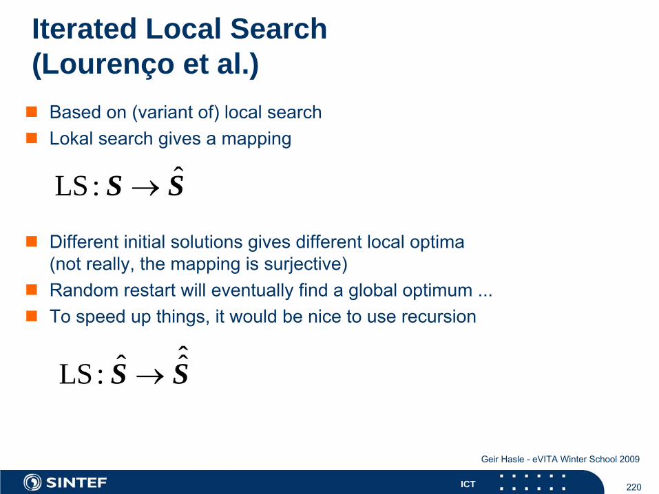
220ICT
Geir Hasle - eVITA Winter School 2009
Iterated Local Search (Lourenço et al.)
Based on (variant of) local searchLokal search gives a mapping
ˆLS: →S S
Different initial solutions gives different local optima (not really, the mapping is surjective)Random restart will eventually find a global optimum ...To speed up things, it would be nice to use recursion
ˆˆ ˆLS: →S S
221ICT
Geir Hasle - eVITA Winter School 2009
Iterated Local Search
Try to iterate in such a way that we do not enter the same ”Basin of attraction”Perturbation of the current solutionDiversification
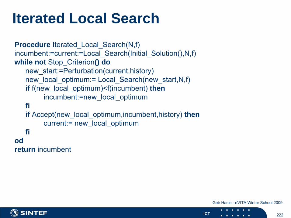
222ICT
Geir Hasle - eVITA Winter School 2009
Iterated Local SearchProcedure Iterated_Local_Search(N,f)incumbent:=current:=Local_Search(Initial_Solution(),N,f)while not Stop_Criterion() do
new_start:=Perturbation(current,history)new_local_optimum:= Local_Search(new_start,N,f)if f(new_local_optimum)<f(incumbent) then
incumbent:=new_local_optimumfiif Accept(new_local_optimum,incumbent,history) then
current:= new_local_optimumfi
odreturn incumbent
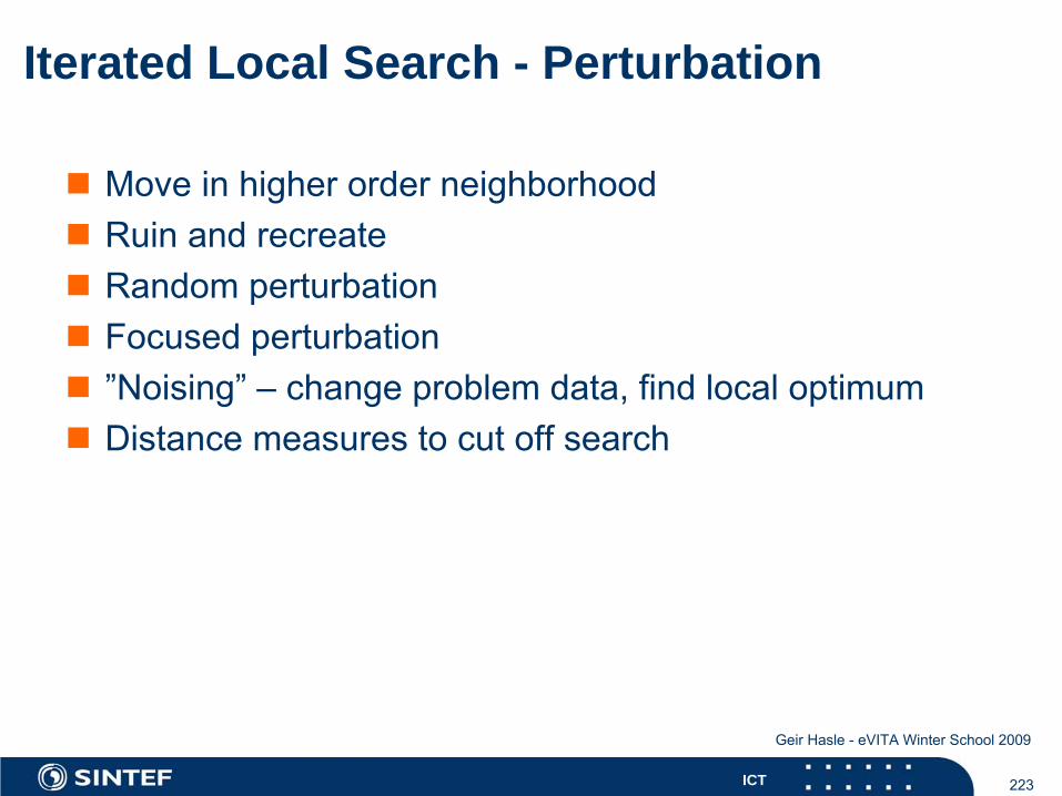
223ICT
Geir Hasle - eVITA Winter School 2009
Iterated Local Search - Perturbation
Move in higher order neighborhoodRuin and recreateRandom perturbationFocused perturbation”Noising” – change problem data, find local optimumDistance measures to cut off search
224ICT
Geir Hasle - eVITA Winter School 2009
Iterated Local Search - Perturbation
How big?Too small: same ”Basin of attraction”Too big: ”Random restart”Varying size
225ICT
Geir Hasle - eVITA Winter School 2009
(Very) Large Neighborhood Search (P. Shaw 1999)
Local Search based methods are often too localGood diversification is essentialLarge Neigborhood Search
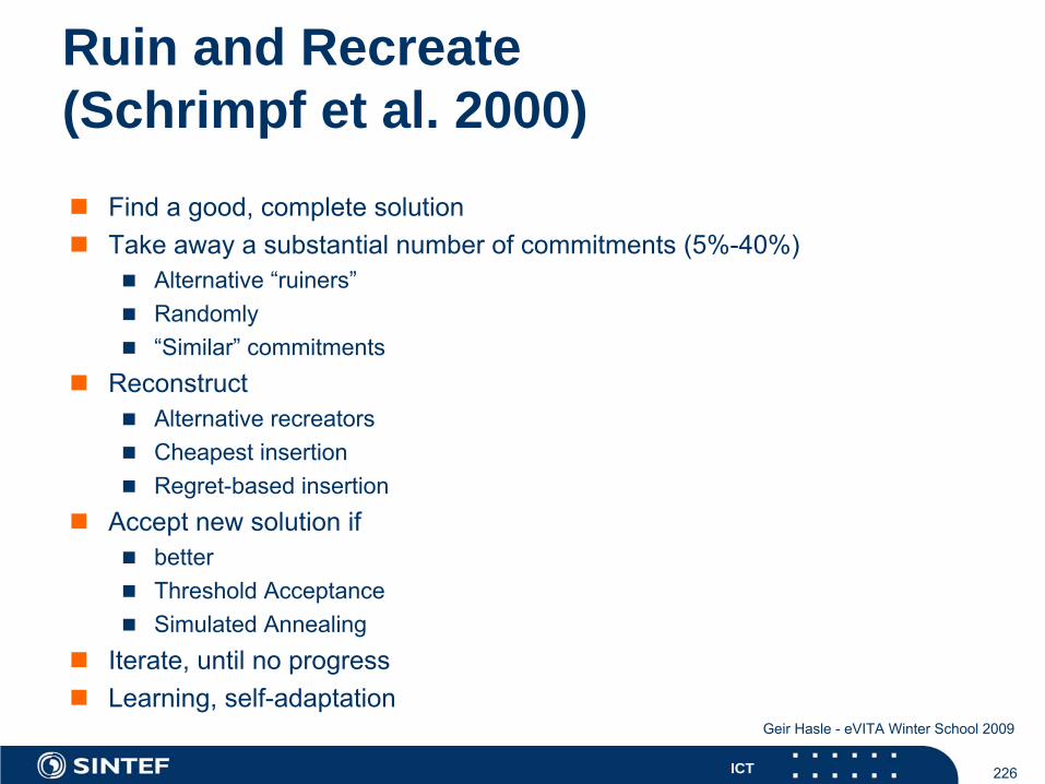
226ICT
Geir Hasle - eVITA Winter School 2009
Find a good, complete solutionTake away a substantial number of commitments (5%-40%)
Alternative “ruiners”Randomly“Similar” commitments
Reconstruct Alternative recreatorsCheapest insertionRegret-based insertion
Accept new solution ifbetterThreshold AcceptanceSimulated Annealing
Iterate, until no progressLearning, self-adaptation
Ruin and Recreate (Schrimpf et al. 2000)
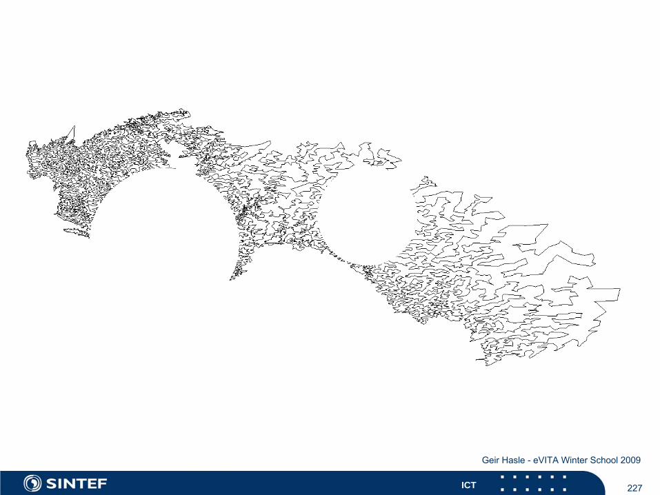
227ICT
Geir Hasle - eVITA Winter School 2009
228ICT
Geir Hasle - eVITA Winter School 2009
Categorization of metaheuristics
Trajectory vs. populationStochastic vs. deterministicMemoryless vs. ”memorable”Restart vs. one shotPenalty-based
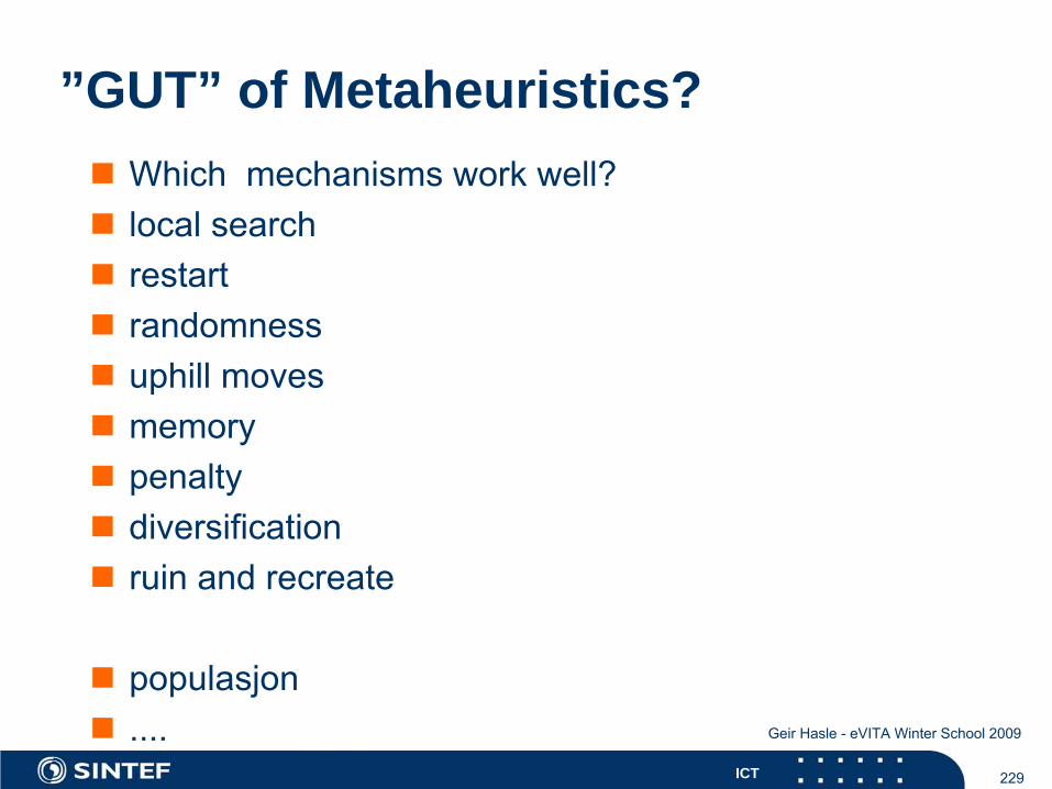
229ICT
Geir Hasle - eVITA Winter School 2009
”GUT” of Metaheuristics?Which mechanisms work well?local searchrestartrandomnessuphill movesmemorypenaltydiversificationruin and recreate
populasjon....
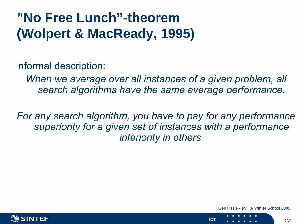
230ICT
Geir Hasle - eVITA Winter School 2009
”No Free Lunch”-theorem (Wolpert & MacReady, 1995)
Informal
description:When
we
average
over all instances
of
a given problem, all
search
algorithms
have the
same average
performance.
For any search algorithm, you have to pay for any performance superiority for a given set of instances with a performance
inferiority in others.
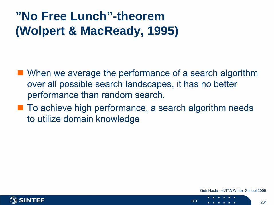
231ICT
Geir Hasle - eVITA Winter School 2009
”No Free Lunch”-theorem (Wolpert & MacReady, 1995)
When we average the performance of a search algorithmover all possible search landscapes, it has no betterperformance than random search. To achieve high performance, a search algorithm needsto utilize domain knowledge
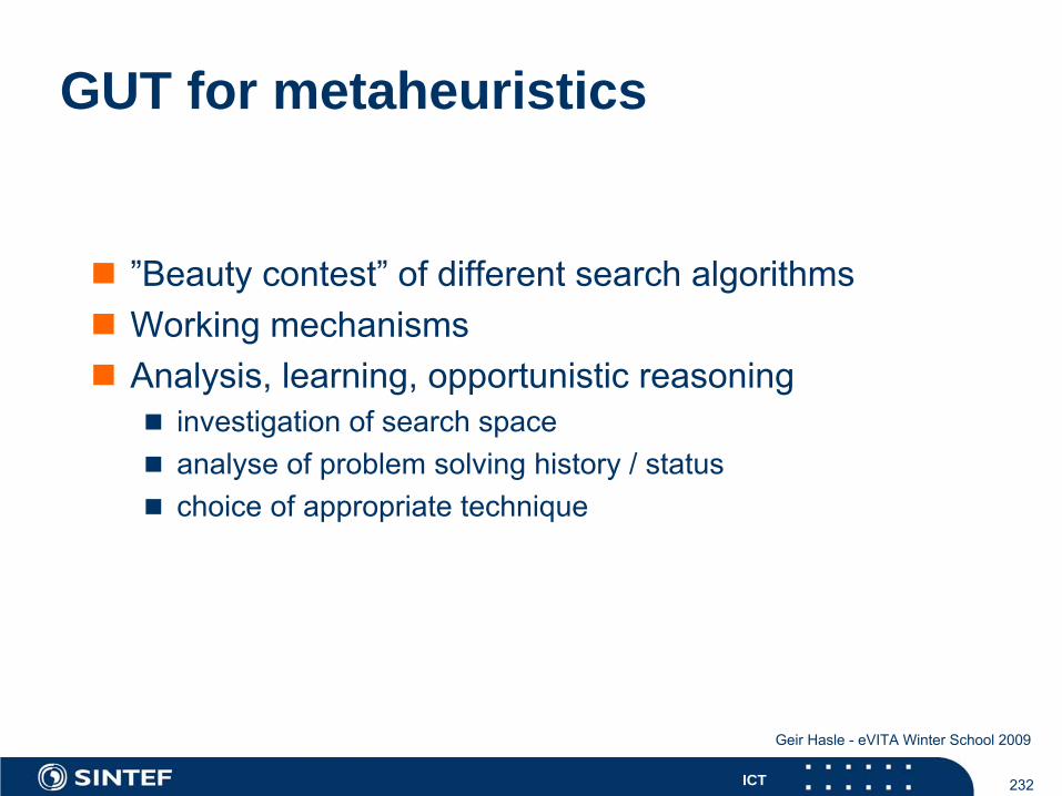
232ICT
Geir Hasle - eVITA Winter School 2009
GUT for metaheuristics
”Beauty contest” of different search algorithmsWorking mechanismsAnalysis, learning, opportunistic reasoning
investigation of search spaceanalyse of problem solving history / statuschoice of appropriate technique
233ICT
Geir Hasle - eVITA Winter School 2009
Hyperheuristics
Metaheuristics are not genericThere is no globally best metaheuristicHyperheuristics
General search techniquesBased on (meta)heuristicsUse of (meta)heuristics to select (meta)heuristic during searchno use of domain knowledge
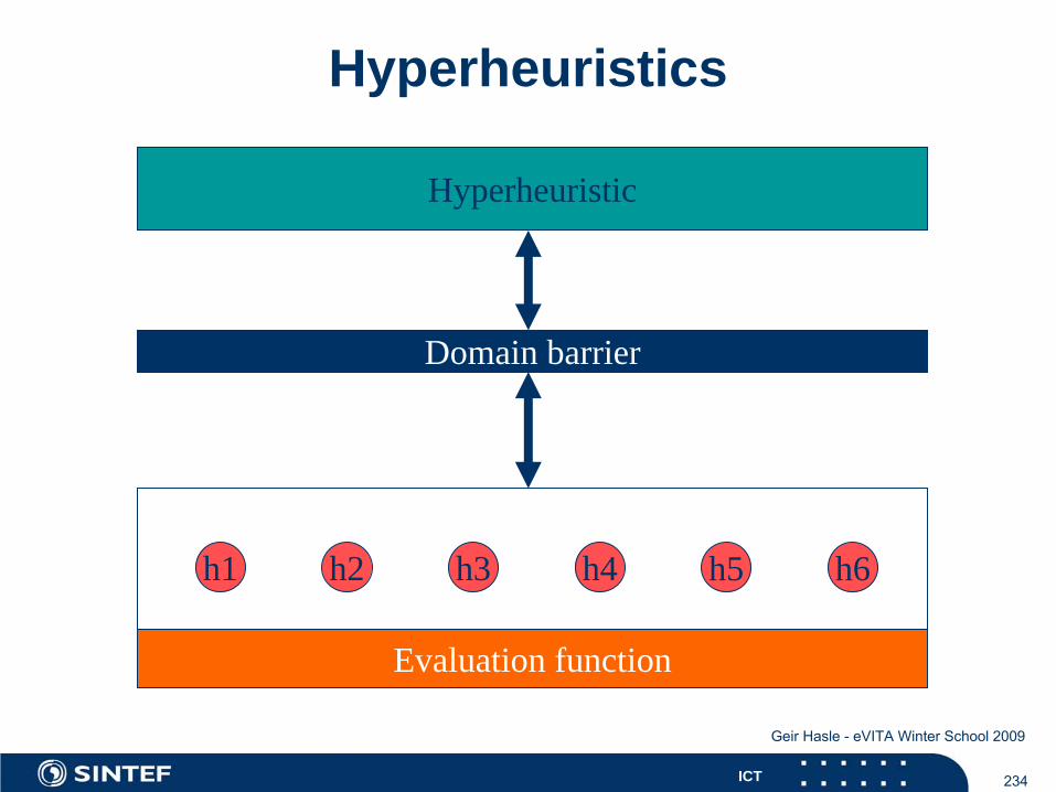
234ICT
Geir Hasle - eVITA Winter School 2009
Hyperheuristics
h1
Evaluation function
h2 h3 h4 h5 h6
Domain barrier
Hyperheuristic
235ICT
Geir Hasle - eVITA Winter School 2009
Hyperheuristics
General information to hyperheuristic from each(meta)heuristicCPU timeMerit, improvement of objective over timeHow long since last active

236ICT
Geir Hasle - eVITA Winter School 2009
Topics for future research
Hybrid methodsCombination of exact and heuristic methodsParallel algorithmsCollaborating solversSelf-adaptive methods, hyperheuristics
Theoretical understanding of search algorithms

237ICT
Geir Hasle - eVITA Winter School 2009
Summary (slide 1)
Discrete optimization problems are importantDiscrete optimization problems are often computationallyhardExact methods may take too long, will give guaranteesBetter to find a good solution to the real problem than theoptimal problem to an overly idealized problemLocal Search is a robust, simple and fast methodLocal Search gives few and weak guaranteesLocal Search is local, gets trapped in a local optimum
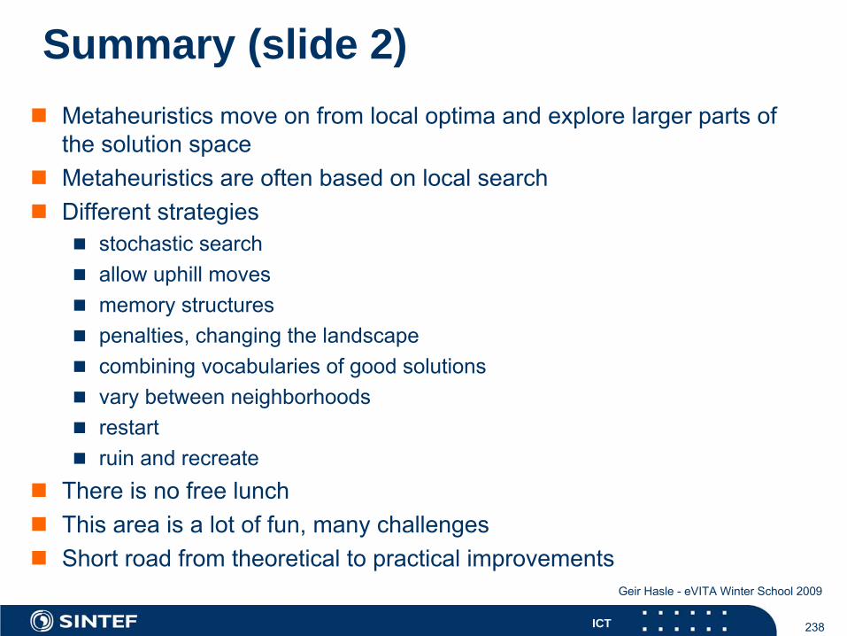
238ICT
Geir Hasle - eVITA Winter School 2009
Summary (slide 2)Metaheuristics move on from local optima and explore larger parts ofthe solution spaceMetaheuristics are often based on local searchDifferent strategies
stochastic searchallow uphill movesmemory structurespenalties, changing the landscapecombining vocabularies of good solutionsvary between neighborhoodsrestartruin and recreate
There is no free lunchThis area is a lot of fun, many challengesShort road from theoretical to practical improvements

239ICT
Geir Hasle - eVITA Winter School 2009
Discrete Optimization - Heuristics
Geir HasleSINTEF ICT, Applied Mathematics
University of Jyväskylä, Finland