Discrete Mathematical Analysis: theory and geophysical applications.
86
Discrete Mathematical Analysis: theory and geophysical applications
-
Upload
benedict-barber -
Category
Documents
-
view
222 -
download
0
Transcript of Discrete Mathematical Analysis: theory and geophysical applications.
Discrete Mathematical Analysis:
theory and geophysical applications
DMA definition
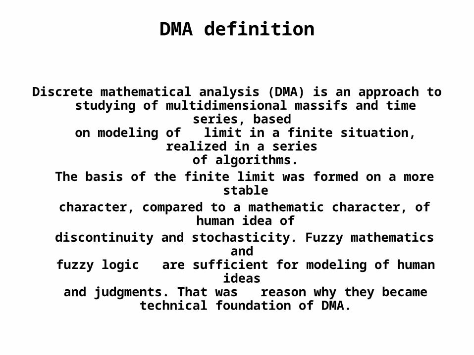
Discrete mathematical analysis (DMA) is an approach to studying of multidimensional massifs and time series, based
on modeling of limit in a finite situation, realized in a series of algorithms.
The basis of the finite limit was formed on a more stable character, compared to a mathematic character, of human idea of
discontinuity and stochasticity. Fuzzy mathematics and fuzzy logic are sufficient for modeling of human ideas
and judgments. That was reason why they became technical foundation of DMA.

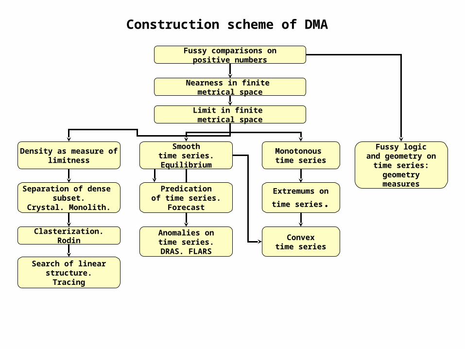
Construction scheme of DMA
Fussy comparisons onpositive numbers
Nearness in finite metrical space
Limit in finite metrical space
Density as measure oflimitness
Smoothtime series.Equilibrium
Monotonous time series
Fussy logicand geometry on
time series:geometrymeasures
Separation of dense subset.
Crystal. Monolith.
Clasterization.Rodin
Predicationof time series.
Forecast
Anomalies ontime series.
DRAS. FLARS
Extremums on
time series.
Convextime series
Search of linearstructure.Tracing
Fuzzy comparisons
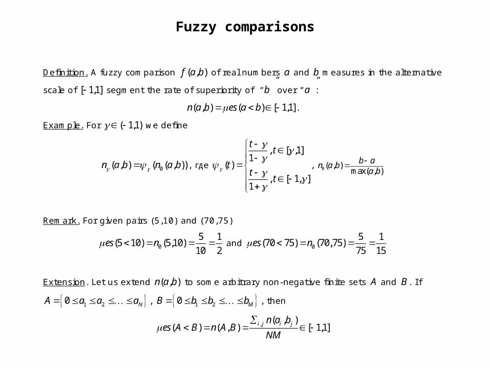
Definition. A fuzzy comparison ( , )f a b of real numbers a and b measures in the alternative
scale of [ 1,1] segment the rate of superiority of “b” over “a ”:
( , ) ( ) [ 1,1]n a b es a b .
Example. For ( 1,1) we define
0( , ) ( ( , ))n a b n a b , где
, [ ,1]1
( )
, [ 1, ]1
tt
tt
t
, 0( , )max( , )
b an a ba b
Remark. For given pairs (5,10) and (70,75)
0
5 1(5 10) (5,10)
10 2es n and 0
5 1(70 75) (70,75)
75 15es n
Extension. Let us extend ( , )n a b to some arbitrary non-negative finite sets A and B . I f
1 20 NA a a a , 1 20 MB b b b , then
, ( , )( ) ( , ) [ 1,1]i j i jn a b
es A B n A BNM
Measures of nearness
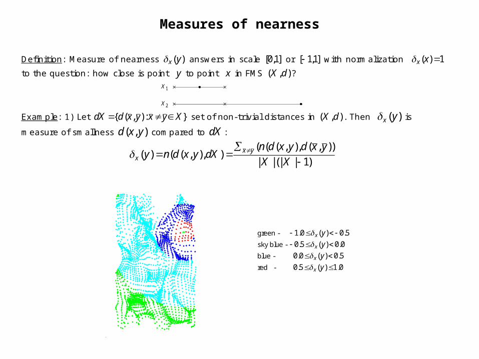
green - 1.0 ( ) 0.5x y
sky blue - 0.5 ( ) 0.0x y
blue - 0.0 ( ) 0.5x y
red - 0.5 ( ) 1.0x y
Definition: Measure of nearness ( )x y answers in scale [0,1] or [ 1,1] with normalization ( ) 1x x
to the question: how close is point y to point x in FMS ( , )X d ? X 1
X 2 Example: 1) Let { ( , ): }dX d x y x y X set of non-trivial distances in ( , )X d . Then ( )x y is
measure of smallness ( , )d x y compared to dX :
( ( ( , ), ( , ))
( ) ( ( , ), )| | (| | 1)
x yx
n d x y d x yy n d x y dX
X X
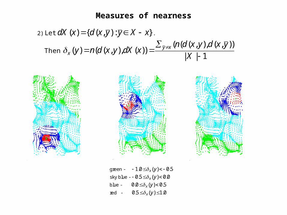
Measures of nearness
2) Let ( ) { ( , ) : }dX x d x y y X x .
Then ( ( ( , ), ( , ))
( ) ( ( , ), ( ))| | 1
y xx
n d x y d x yy n d x y dX x
X
green - 1.0 ( ) 0.5x y
sky blue - 0.5 ( ) 0.0x y
blue - 0.0 ( ) 0.5x y
red - 0.5 ( ) 1.0x y
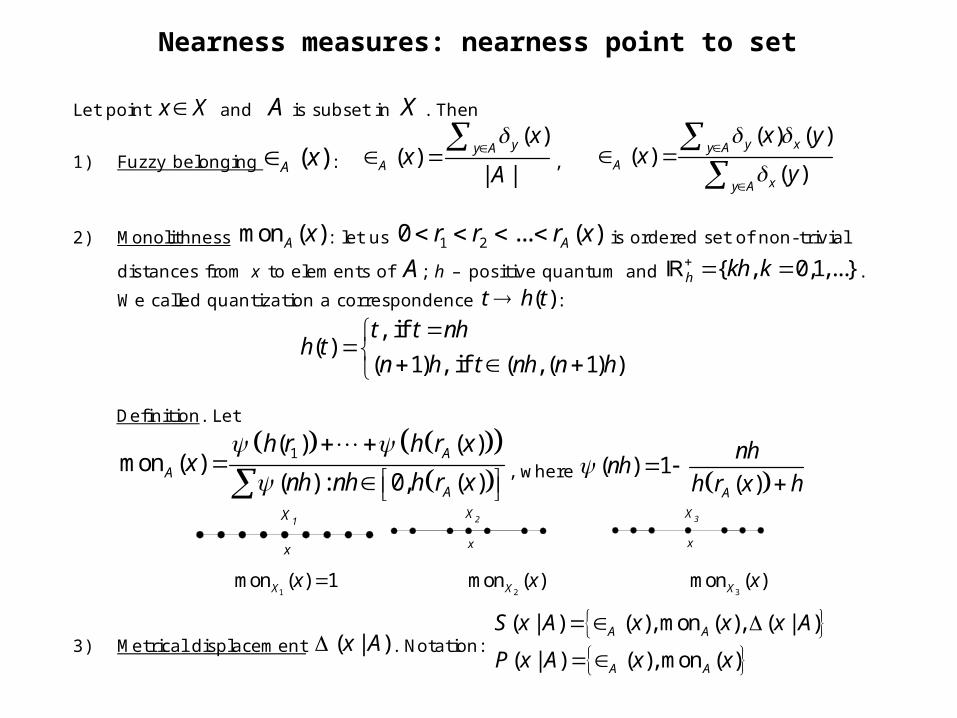
Nearness measures: nearness point to set
Let point x X and A is subset in X . Then
1) Fuzzy belonging ( )A x : ( )
( )| |
yy AA
xx
A
,
( ) ( )( )
( )
y xy AA
xy A
x yx
y
2) Monolithness mon ( )A x : let us 1 20 ... ( )Ar r r x is ordered set of non-trivial
distances from x to elements of A ; h – positive quantum and { , 0,1,...}h kh k .
We called quantization a correspondence ( )t h t :
, if ( )
( 1) , if ( , ( 1) )
t t nhh t
n h t nh n h
Definition. Let
1( ) ( )mon ( )
( ) : 0, ( )A
AA
h r h r xx
nh nh h r x
, where ( ) 1
( )A
nhnh
h r x h
x
X 1
x
X 2
x
X 3
1mon ( ) 1X x >
2mon ( )X x >
3mon ( )X x
3) Metrical displacement ( | )x A . Notation:
( | ) ( ), mon ( ), ( | )
( | ) ( ), mon ( )
A A
A A
S x A x x x A
P x A x x
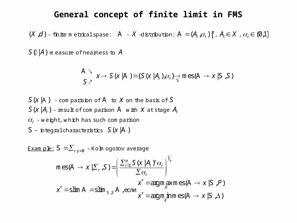
General concept of finite limit in FMS
( , )X d - finite metrical spase: A - X -distribution: 1( , ) |ni iA A , iA X , (0,1]i
( | )S A measure of nearness to A
( | ) { ( | ), } mes( | , )i ix S x S x A x SS
AA A
SS
( | )S x A - comparision of A to x on the basis of S
( | )iS x A - result of comparison A with x at stage iA
i - weight, which has such comparison
S – integral characteristics ( | )S x A
Example: , 0 S - Kolmogorov average
1
1 ( | )mes( | , )
ni ii
i
S x Ax S
A
*
*, *
еслиargmax mes( | , )
slim slim ,argmin mes( | , )
XS
X
x x Px
x x
S
S
S
AA A
A

Construction scheme of DMA
Fussy comparisons onpositive numbers
Nearness in finite metrical space
Limit in finite metrical space
Density as measure oflimitness
Smoothtime series.Equilibrium
Monotonous time series
Fussy logicand geometry on
time series:geometrymeasures
Separation of dense subset.
Crystal. Monolith.
Clasterization.Rodin
Predicationof time series.
Forecast
Anomalies ontime series.
DRAS. FLARS
Extremums on
time series.
Convextime series
Search of linearstructure.Tracing
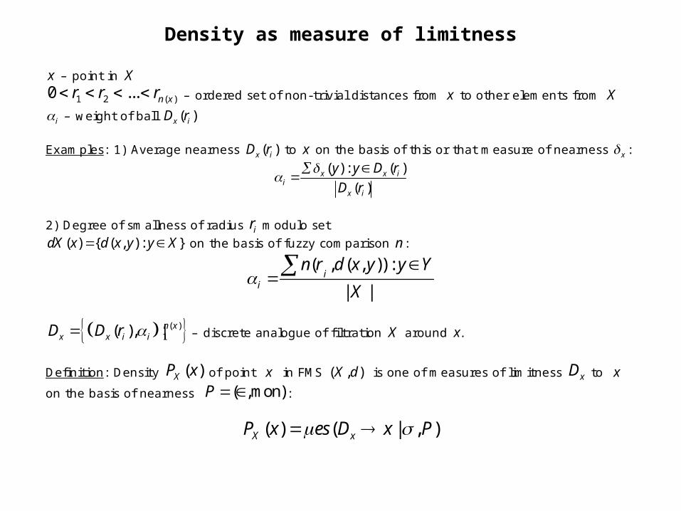
Density as measure of limitness
x – point in X
1 2 ( )0 ... n xr r r – ordered set of non-trivial distances from x to other elements from X
i – weight of ball ( )x iD r Examples: 1) Average nearness ( )x iD r to x on the basis of this or that measure of nearness x :
( ) : ( )
( )x x i
ix i
y y D r
D r
2) Degree of smallness of radius ir modulo set
( ) { ( , ) : }dX x d x y y X on the basis of fuzzy comparison n :
( , ( , )) :
| |i
i
n r d x y y Y
X
( )1( ), |n x
x x i iD D r – discrete analogue of filtration X around x .
Definition: Density ( )XP x of point x in FMS ( , )X d is one of measures of limitness xD to x
on the basis of nearness ( ,mon)P :
( ) ( | , )X xP x es D x P
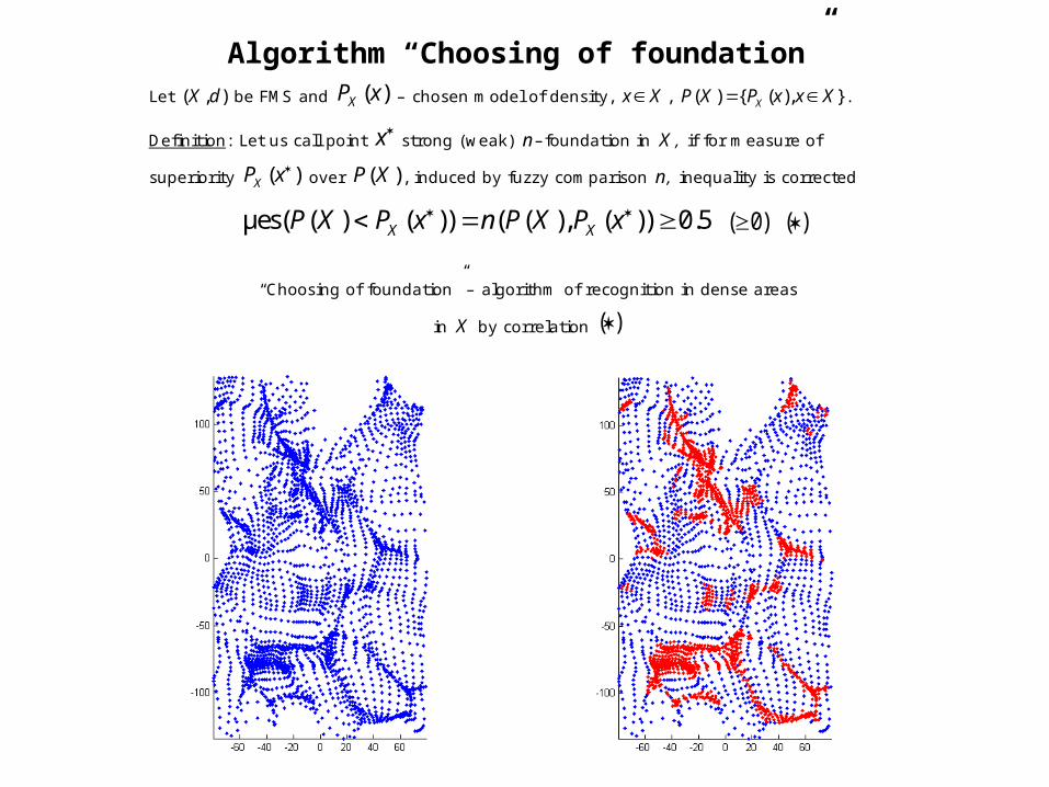
Algorithm “Choosing of foundation”Let ( , )X d be FMS and ( )XP x – chosen model of density, x X , ( ) { ( ), }XP X P x x X .
Definition: Let us call point x strong (weak) n – foundation in X , if for measure of
superiority ( )XP x over ( )P X , induced by fuzzy comparison n , inequality is corrected
μes( ( ) ( )) ( ( ), ( )) 0.5X XP X P x n P X P x ( 0) ( )
“Choosing of foundation” – algorithm of recognition in dense areas
in X by correlation ( )
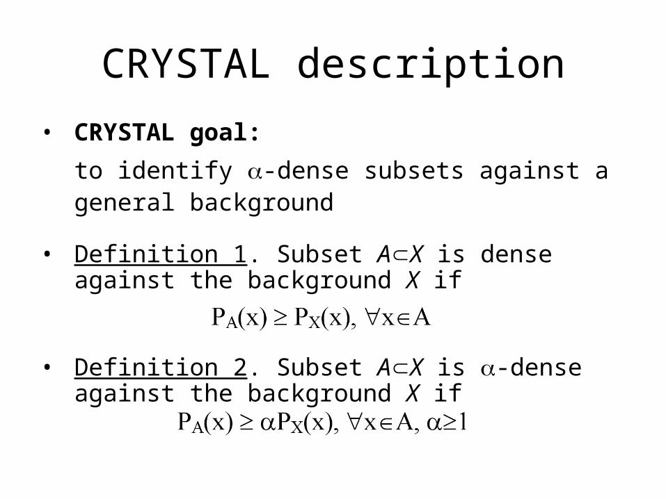
CRYSTAL description
• CRYSTAL goal:
to identify -dense subsets against a general background
• Definition 1. Subset AX is dense against the background X if
• Definition 2. Subset AX is -dense against the background X if
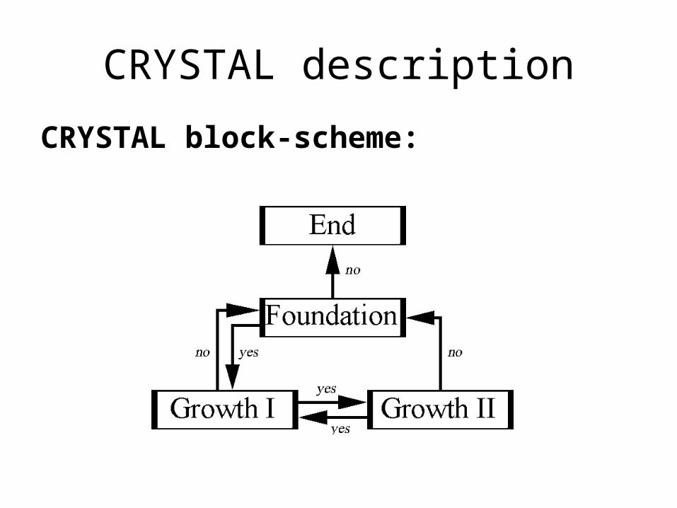
CRYSTAL description
CRYSTAL block-scheme:
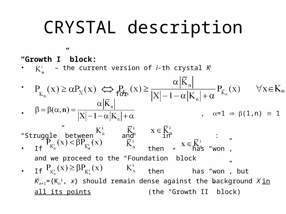
CRYSTAL description
“Growth I” block:• – the current version of i-th crystal Ki
• for
• , =1 (1,n) 1
“Struggle” between and in :
• If then has “won”, and we proceed to the “Foundation” block
• If then has “won”, but Kin+1={Kn
i, x} should
remain dense against the background X in all its points (the “Growth II” block)
CRYSTAL description
“Growth II” block (1):• Statement. If the “Growth I” condition is fulfilled then Kn+1={Kn, xn+1}
will be -dense only if the “Growth II” condition is fulfilled:
=1
• If there is no such xn+1, we proceed to the “Foundation” block for
choosing another foundation for the next crystallization
• If there are several such xn+1 ( ), then
CRYSTAL description
“Growth II” block (2):
• Recalculation of the densities and in for their further “struggle” in the “Growth I” block:
CRYSTAL description
“End” block:
• Identification of the final crystal versions K1, …, KI,
I = I(F,).
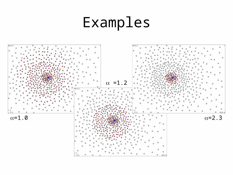
Examples
=1.0
=1.2
=2.3
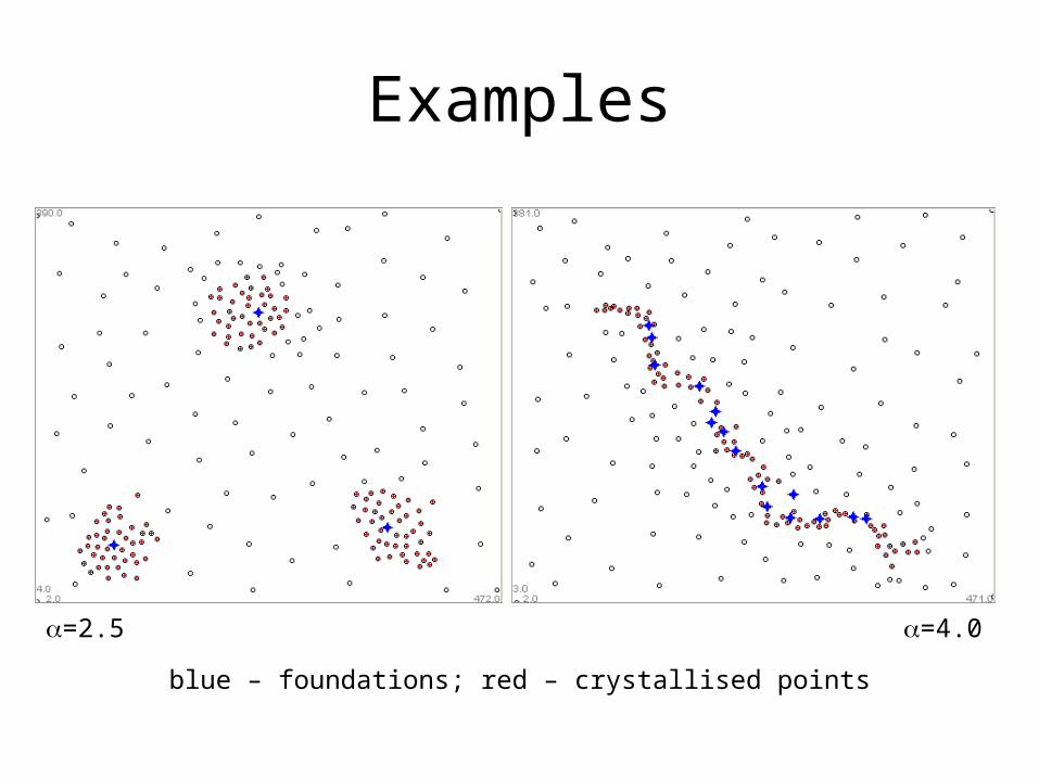
Examples
=2.5 =4.0
blue – foundations; red – crystallised points
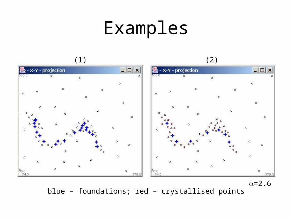
Examples
blue – foundations; red – crystallised points
(1) (2)
=2.6
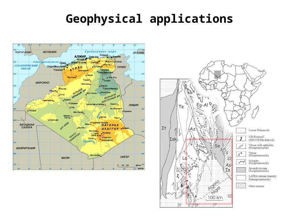
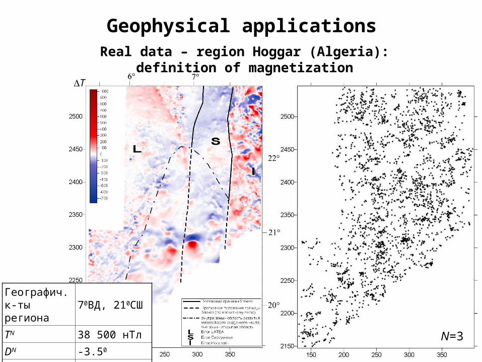
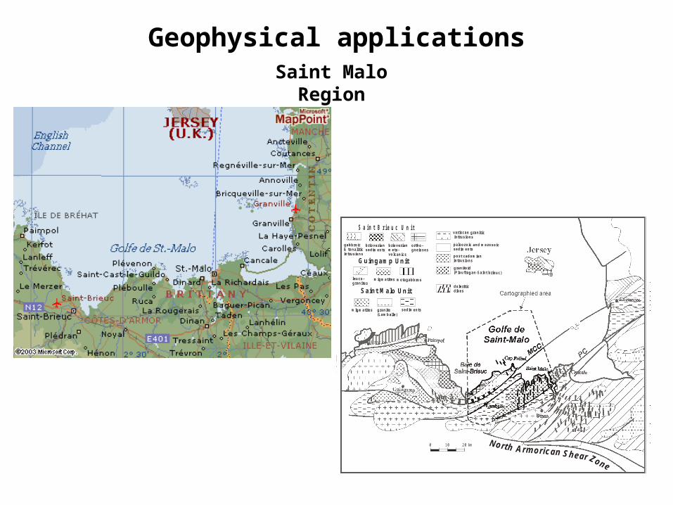
Geophysical applications
Geophysical applications
N=3
Географич. к-ты региона
70ВД, 210СШ
TN 38 500 нТл
DN -3.50
IN 250
Real data – region Hoggar (Algeria):definition of magnetization
T
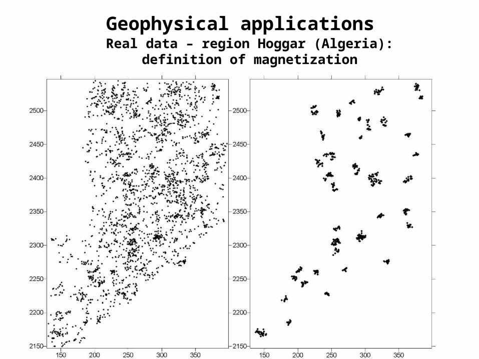
Geophysical applicationsReal data – region Hoggar (Algeria):
definition of magnetization
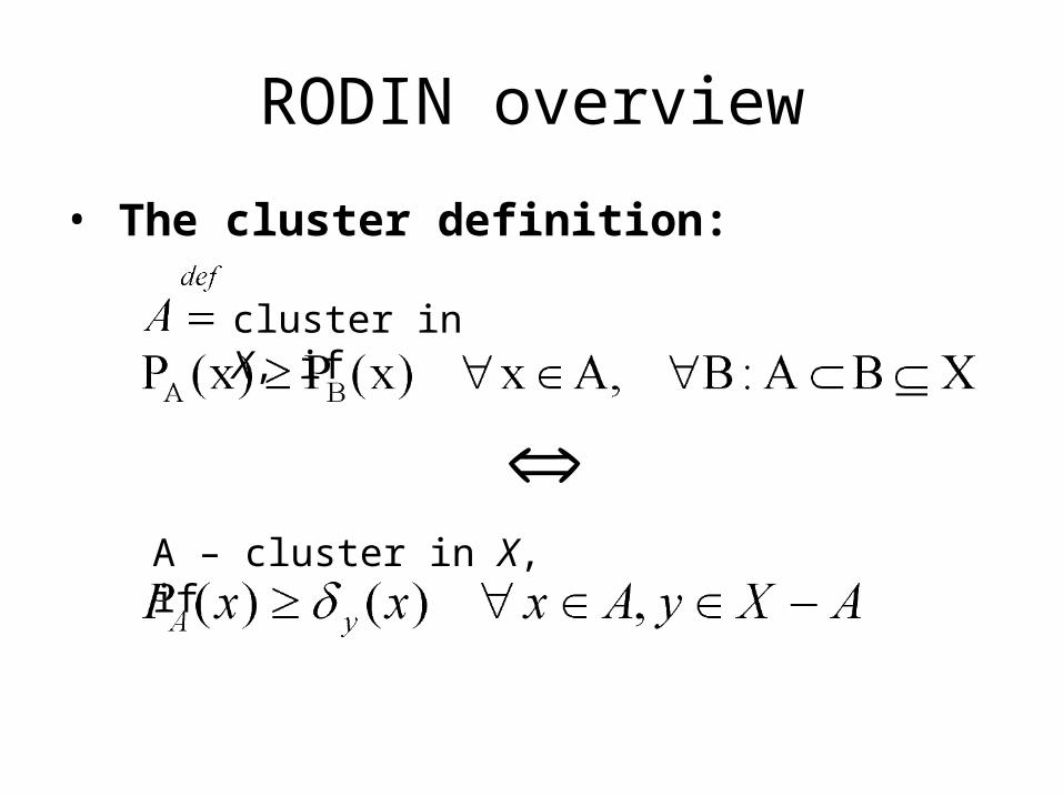
RODIN overview
• The cluster definition:
cluster in X, if
A – cluster in X, if
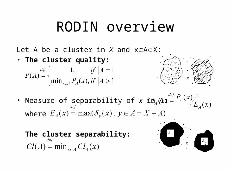
RODIN overview
Let A be a cluster in X and xAX:• The cluster quality:
• Measure of separability of x in A:
where
The cluster separability:
A1 A
2
X
A1
A2X
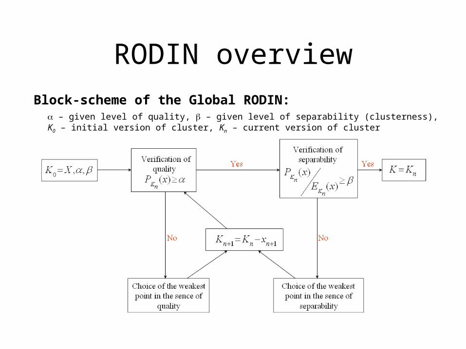
RODIN overview
Block-scheme of the Global RODIN: – given level of quality, – given level of separability (clusterness), K0 – initial version of cluster, Kn – current version of cluster
RODIN overview
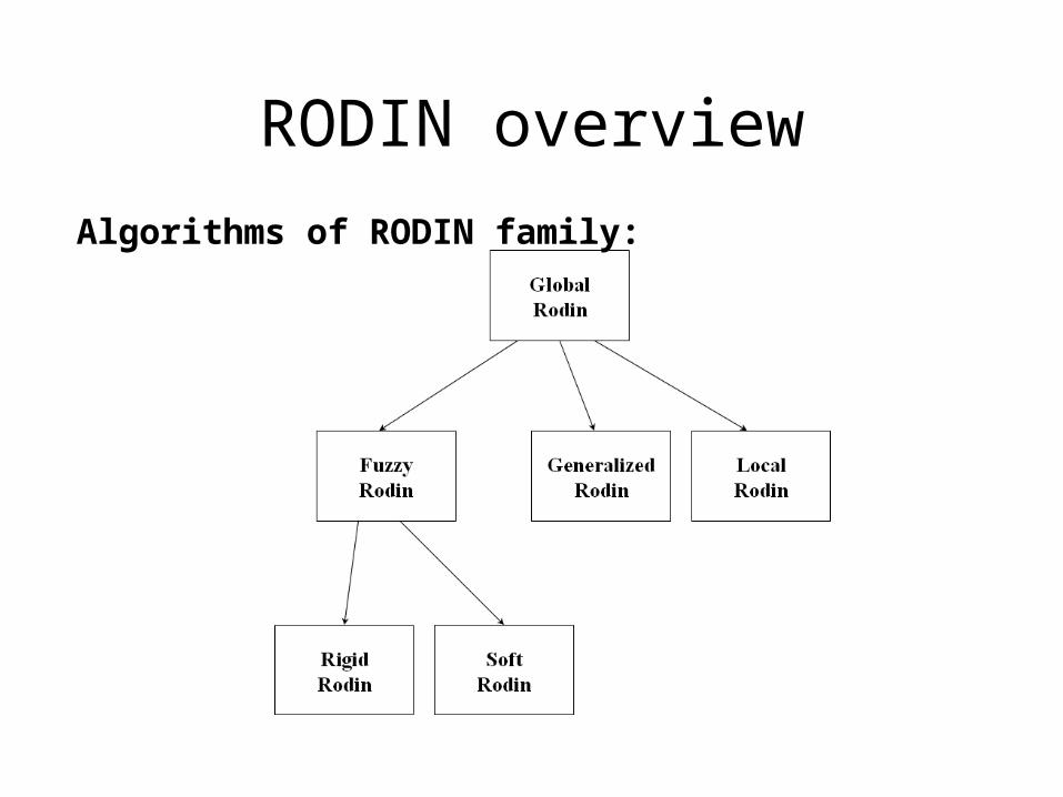
Algorithms of RODIN family:
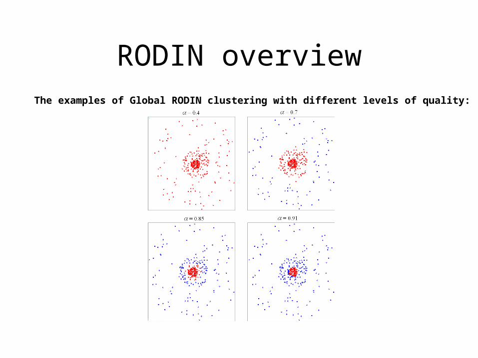
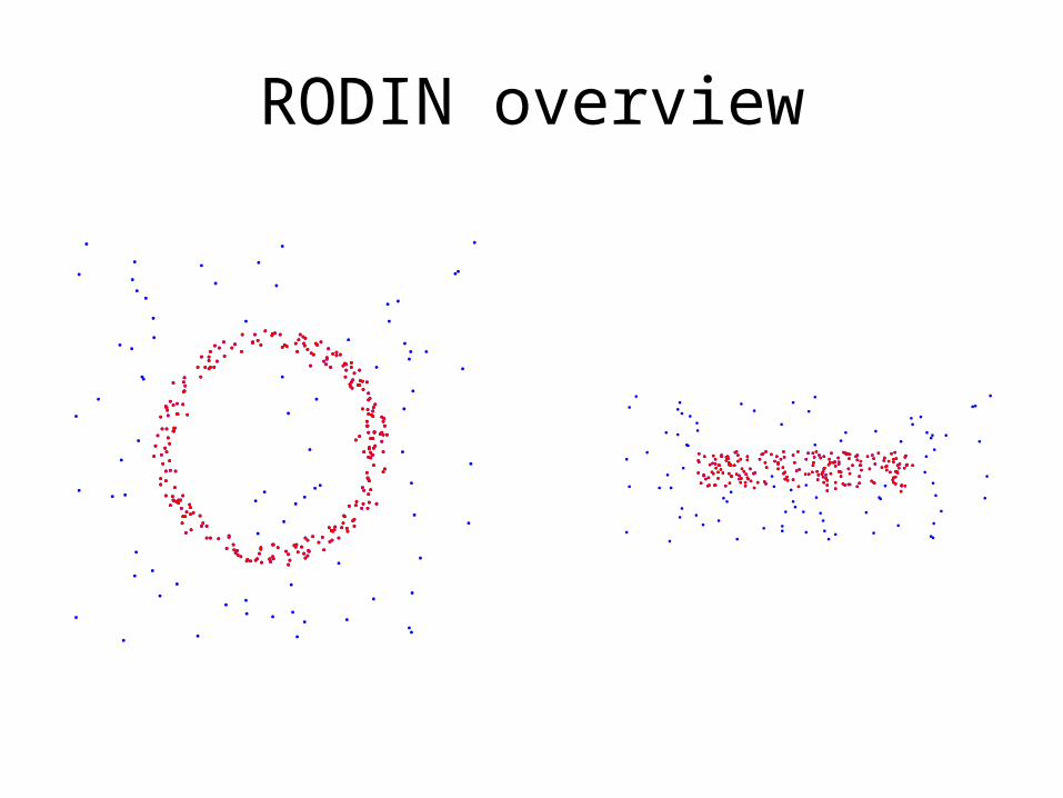
RODIN overviewThe examples of Global RODIN clustering with different levels of quality:
RODIN overview
Geophysical applications
C artographied area
L a n n io n
G u in g a m p
Golfe deSaint-Malo
J ersey
MCCPC
Zone
Shear Armorican
North 0 10 20 km
S a i n t B r i e u c U n i t
ortho-gneisses
brioverian meta-volcanics
brioveriansediments
gabbroic & tonaliticintrusions
Guingamp Unit
metagabbrosmigmatitesleuco-granites
Saint Malo Unit
migmatites granite(Lamballe)
sediments
granitoid (Ploufragan-Saint brieuc)
post cadomian intrusions
paleozoic and mezosoic sediments
variscan granitic intrusions
doleriticdikes
Saint Malo Region
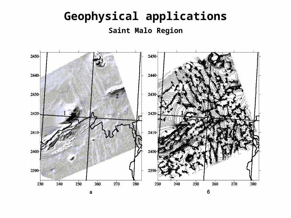
Geophysical applicationsSaint Malo Region
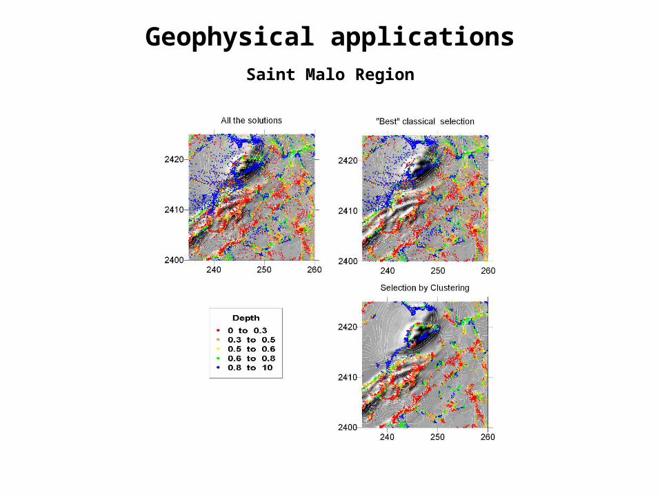
Geophysical applicationsSaint Malo Region
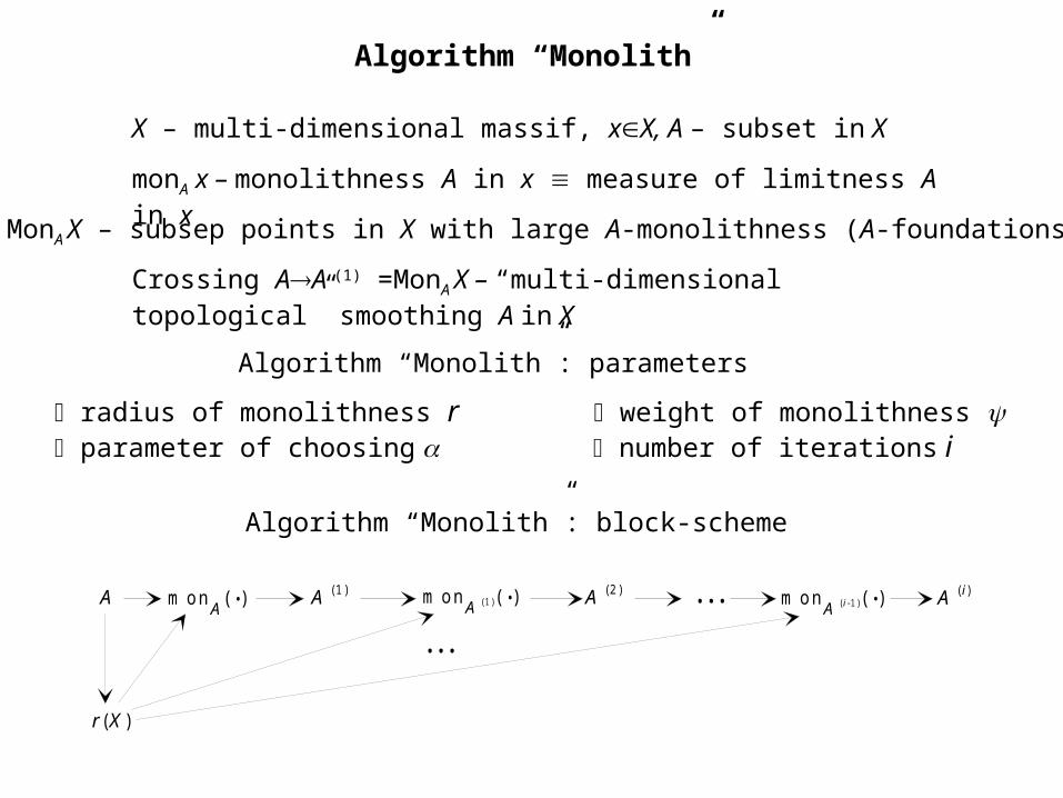
Algorithm “Monolith”
X – multi-dimensional massif, xX, A – subset in X
Crossing AA (1) =MonA X – “multi-dimensional topological” smoothing A in X
MonA X – subsep points in X with large A-monolithness (A-foundations)
radius of monolithness r weight of monolithness parameter of choosing number of iterations i
Algorithm “Monolith”: parameters
monA x – monolithness A in x measure of limitness A in x
Algorithm “Monolith”: block-scheme
A m o n A (. ) A (1 ) m o n A (1 )(. ) A (2 ) A ( i)m o n A ( i-1 )(. )...
r (X )
...
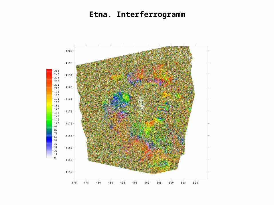
Etna. Interferrogramm
470 475 480 485 490 495 500 505 510 515 520
4150
4155
4160
4165
4170
4175
4180
4185
4190
4195
4200
0102030405060708090100110120130140150160170180190200210220230240250

Smoothness of displacement
Let be a set of pixels, ( ) п - a shift of pixel п measured by satellite, ( )D п - its
neighborhood (it could be neighboring points or a sphere of radius r around pixel п).
There are different variants of smoothness ( )G п of shift in point п . Let’s cite
several examples:
1. ( )G п - average deviation
( ) ( )( )
( )G
D
п п
пп
, ( )Dп п .
A palette was used in our calculations ( )D п - 3х3 and
ï
ï
( ) ( )( )
8G
п п
п
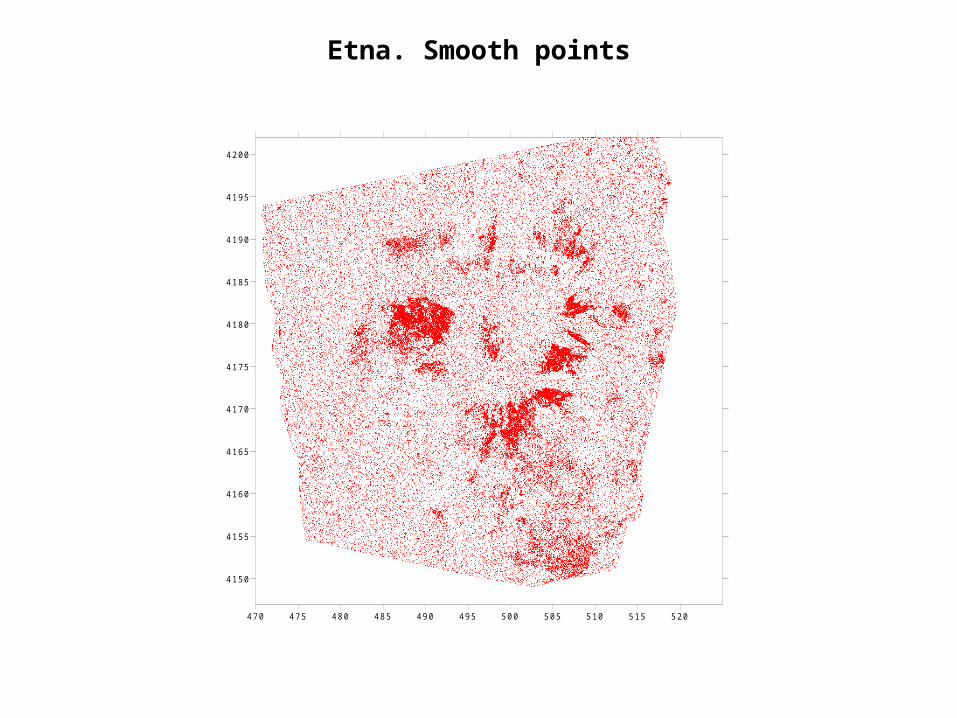
Etna. Smooth points
470 475 480 485 490 495 500 505 510 515 520
4150
4155
4160
4165
4170
4175
4180
4185
4190
4195
4200
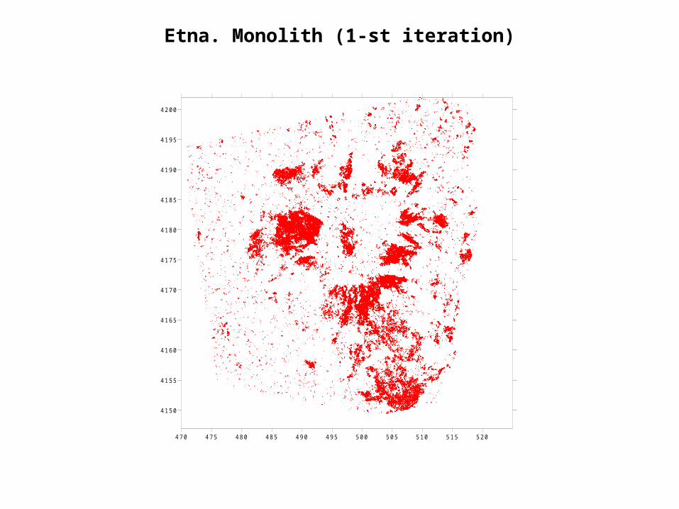
Etna. Monolith (1-st iteration)
470 475 480 485 490 495 500 505 510 515 520
4150
4155
4160
4165
4170
4175
4180
4185
4190
4195
4200
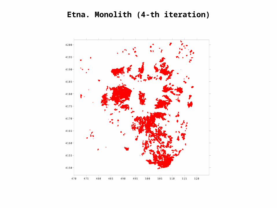
Etna. Monolith (4-th iteration)
470 475 480 485 490 495 500 505 510 515 520
4150
4155
4160
4165
4170
4175
4180
4185
4190
4195
4200
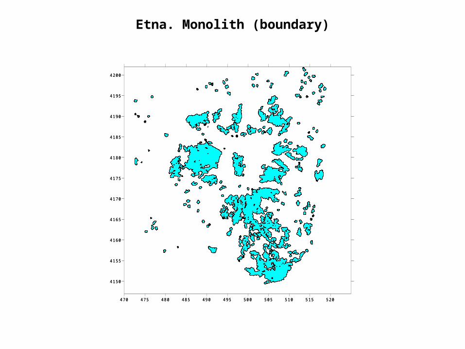
Etna. Monolith (boundary)
470 475 480 485 490 495 500 505 510 515 520
4150
4155
4160
4165
4170
4175
4180
4185
4190
4195
4200
470 475 480 485 490 495 500 505 510 515 520
4150
4155
4160
4165
4170
4175
4180
4185
4190
4195
4200
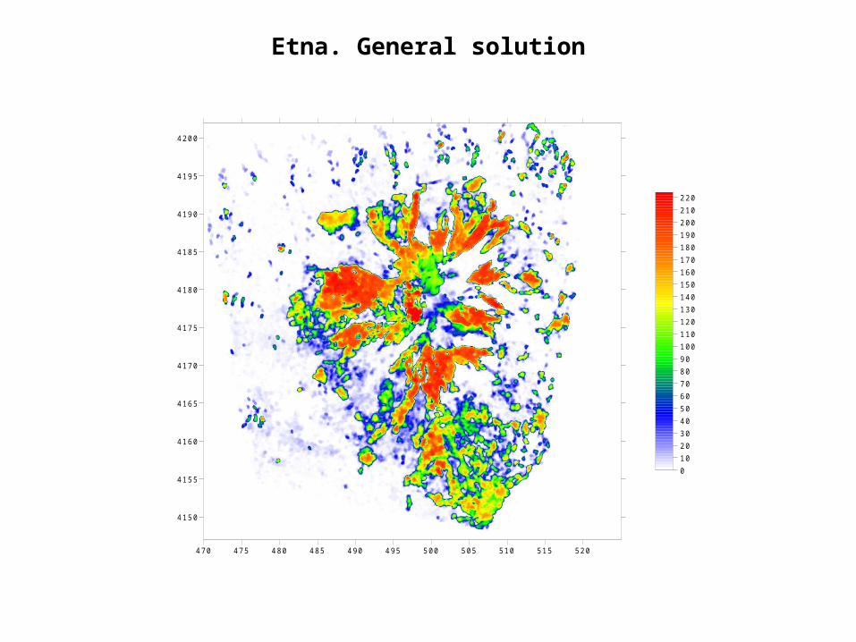
Etna. General solution
470 475 480 485 490 495 500 505 510 515 520
4150
4155
4160
4165
4170
4175
4180
4185
4190
4195
4200
0102030405060708090100110120130140150160170180190200210220
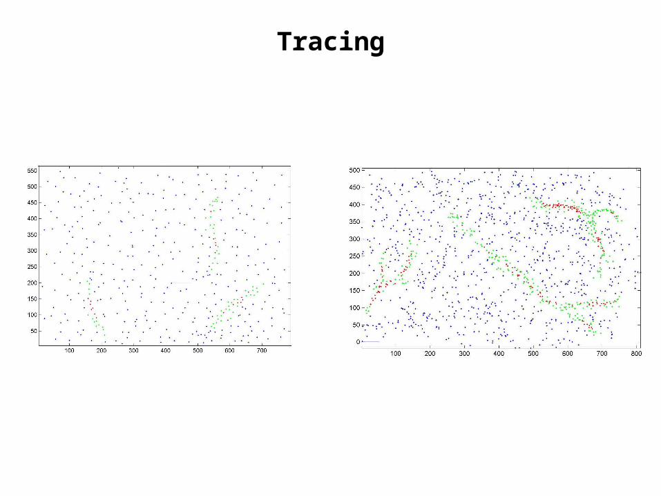
Tracing
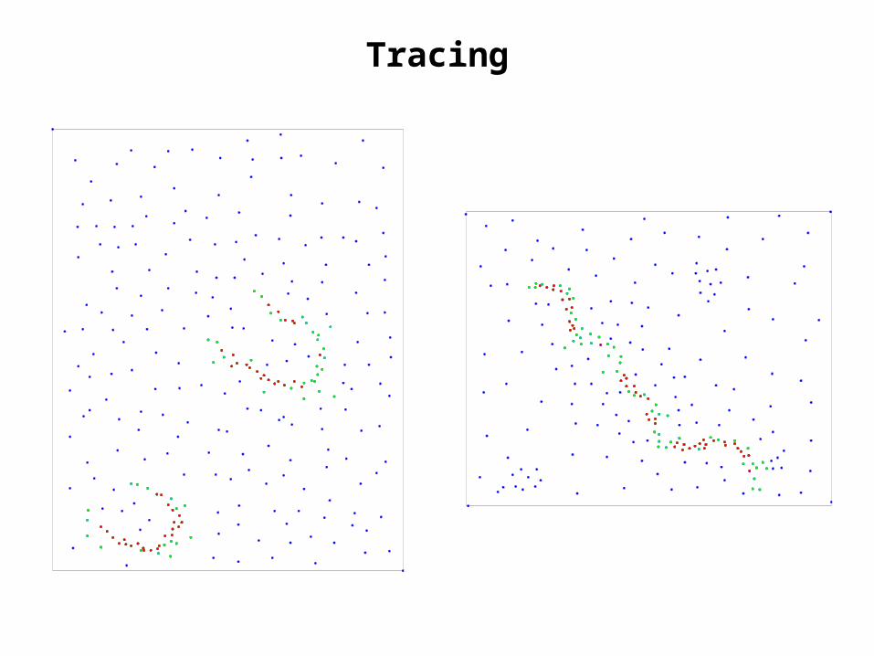
Tracing

Construction scheme of DMA
Fussy comparisons onpositive numbers
Nearness in finite metrical space
Limit in finite metrical space
Density as measure oflimitness
Smoothtime series.Equilibrium
Monotonous time series
Fussy logicand geometry on
time series:geometrymeasures
Separation of dense subset.
Crystal. Monolith.
Clasterization.Rodin
Predicationof time series.
Forecast
Anomalies ontime series.
DRAS. FLARS
Extremums on
time series.
Convextime series
Search of linearstructure.Tracing
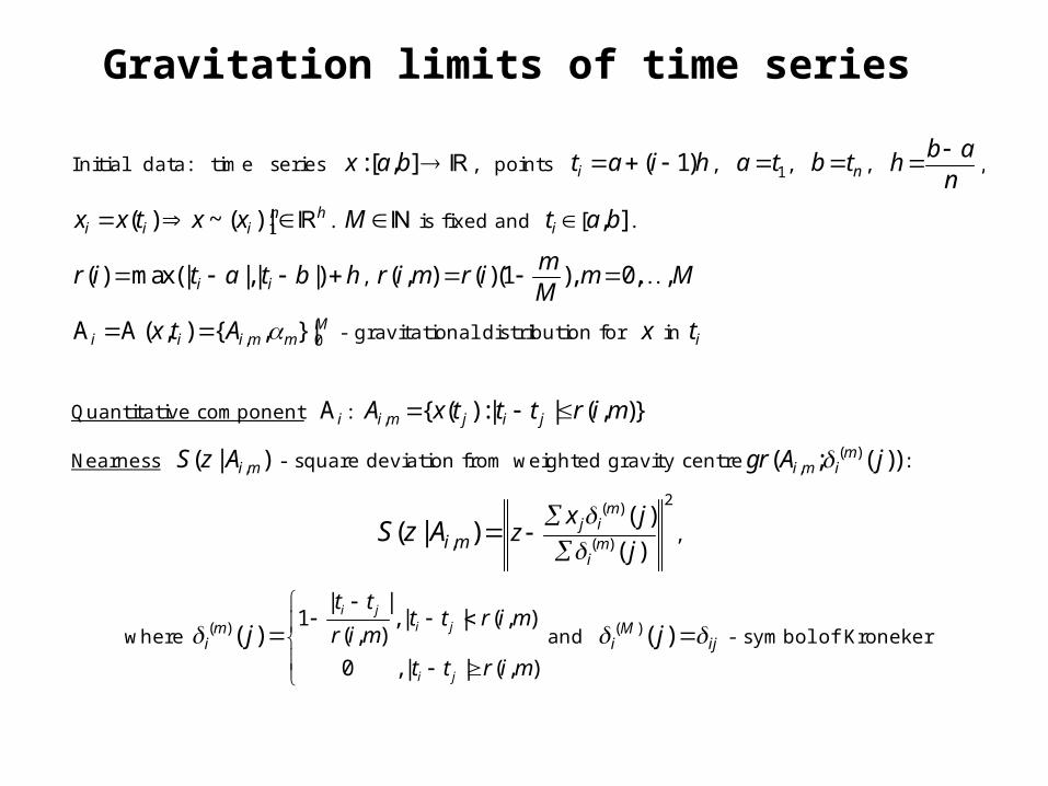
Gravitation limits of time series
Initial data: time series :[ , ]x a b , points ( 1)it a i h , 1a t , nb t , b a
hn ,
1( ) ~ ( ) |n hi i ix x t x x . M is fixed and [ , ]it a b .
( ) max(| |,| |)i ir i t a t b h , ( , ) ( )(1 ), 0, ,m
r i m r i m MM
, 0( , ) { , }|Mi i i m mx t A A A - gravitational distribution for x in it
Quantitative component iA : , { ( ) :| | ( , )}i m j i jA x t t t r i m
Nearness ,( | )i mS z A - square deviation from weighted gravity centre ( ),( ; ( ))m
i m igr A j :
2( )
( ),( )
( )( | )
mj i
mi
i mx j
zj
S z A
,
where ( )
| |1 , | | ( , )
( , )
0 , | | ( , )
( )i j
i j
i j
mi
t tt t r i m
r i m
t t r i m
j
and ( )( )Mi ijj - symbol of Kroneker
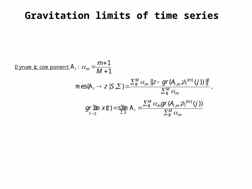
Gravitation limits of time series
Dynamic component iA : 11m
mM
( ) 2,0
0
|| ( ; ( )) ||mes( | , )
mMm i m i
i Mm
z gr A jz S
A ,
( ),0
,0
( ; ( ))lim ( ) slim
i
mMm i m i
i MSt t m
gr A jgr x t
A
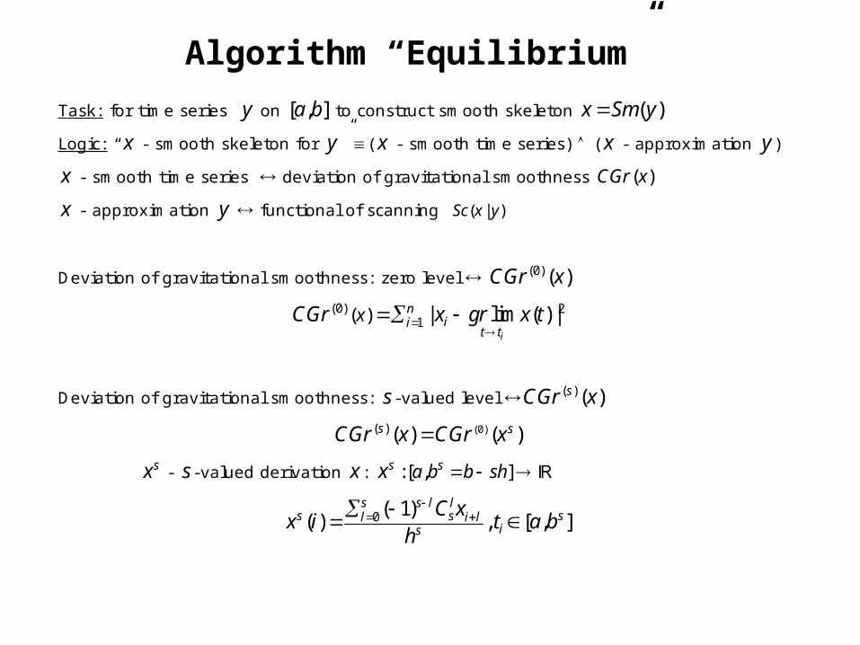
Algorithm “Equilibrium” Task: for time series y on [ , ]a b to construct smooth skeleton ( )x Sm y
Logic: “x - smooth skeleton for y ” ( x - smooth time series) ( x - approximation y )
x - smooth time series deviation of gravitational smoothness ( )CGr x
x - approximation y functional of scanning ( | )Sc x y
Deviation of gravitational smoothness: zero level (0)( )CGr x
(0) 21( ) | lim ( ) |
i
nii
t txCGr x gr x t
Deviation of gravitational smoothness: s -valued level ( )( )sCGr x
(0)( )( ) ( )s sCGr x CGr x
sx - s -valued derivation x : :[ , ]s sa b b shx
0( 1)( ) , [ , ]
s s l ls ssl i l
is
C xx i t a b
h
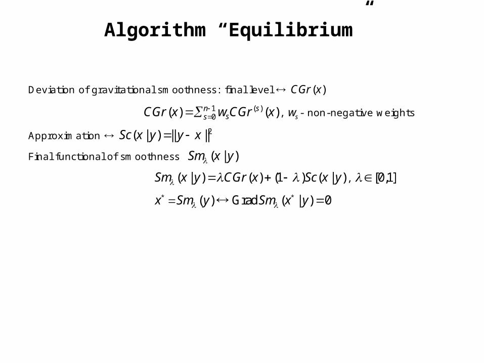
Algorithm “Equilibrium”
Deviation of gravitational smoothness: final level ( )CGr x
( )10( ) ( )sn
ssCGr x w CGr x , sw - non-negative weights
Approximation 2( | ) || ||Sc x y y x
Final functional of smoothness ( | )Sm x y
( | ) ( ) (1 ) ( | )Sm x y CGr x Sc x y , [0,1]
* *( ) Grad ( | ) 0x Sm y Sm x y
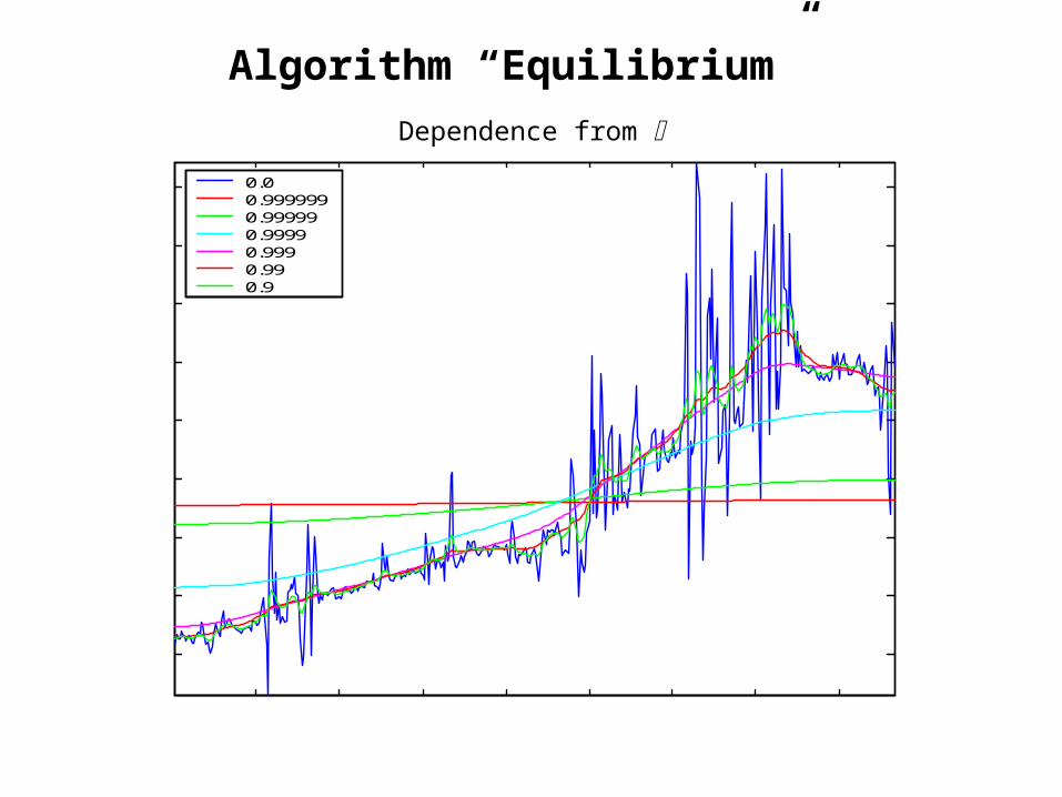
Algorithm “Equilibrium”
0.00.9999990.999990.99990.9990.990.9
Dependence from
Algorithm “Equilibrium”
( ) ( ) (1 ) ( | )Sm x CGr x Sc x y , [0,1] *x Sm y *Grad ( | ) 0Sm x y
10( ) ( )n s
s sCGr x CGr x
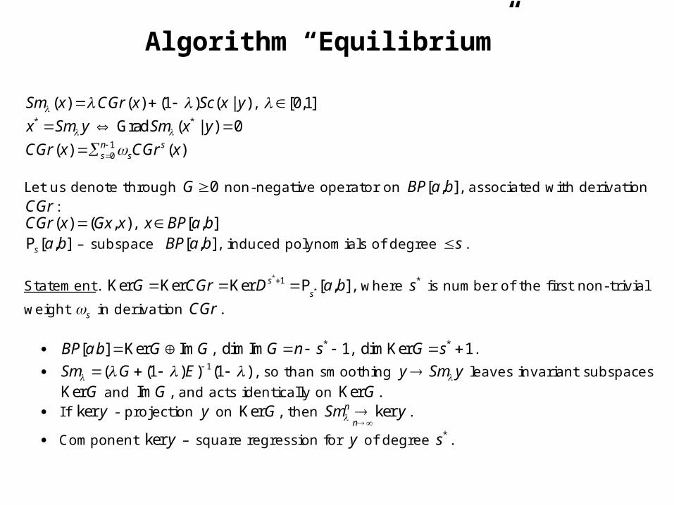
Let us denote through 0G non-negative operator on [ , ]ВР a b , associated with derivation CGr :
( ) ( , )CGr x Gx x , [ , ]x ВР a b
[ , ]s a bP – subspace [ , ]ВР a b , induced polynomials of degree s .
Statement. *
*
1Ker Ker Ker [ , ]s
sG CGr D a b P , where *s is number of the first non-trivial
weight s in derivation CGr .
[ . ] Ker ImВР a b G G , *dimIm 1G n s , *dimKer 1G s .
1( (1 ) ) (1 )Sm G E , so than smoothing y Sm y leaves invariant subspaces
KerG and ImG , and acts identically on KerG . I f ker y - projection y on KerG , then kern
nSm y
.
Component ker y – square regression for y of degree *s .
Algorithm “Equilibrium”
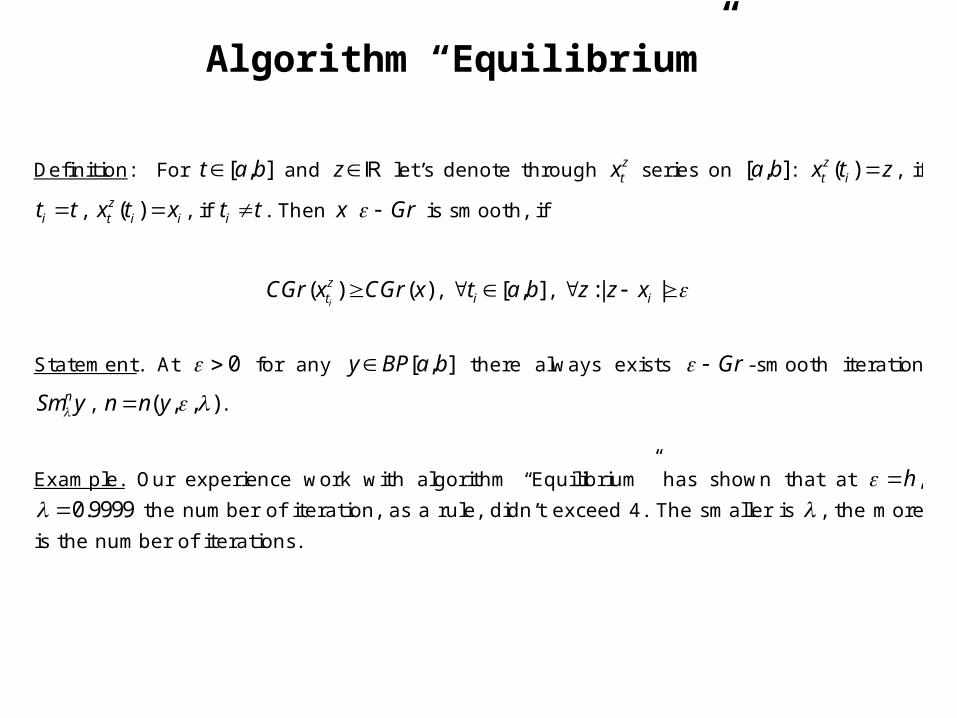
Definition: For [ , ]t a b and z let’s denote through ztx series on [ , ]a b : ( )z
t ix t z , if
it t , ( )zt i ix t x , if it t . Then x Gr is smooth, if
( ) ( )i
ztCGr x CGr x , [ , ]it a b , :| |iz z x
Statement. At 0 for any [ , ]y ВР a b there always exists Gr -smooth iteration
nSm y , ( , , )n n y .
Example. Our experience work with algorithm “Equilibrium” has shown that at h ,
0.9999 the number of iteration, as a rule, didn’t exceed 4. The smaller is , the more
is the number of iterations.
Algorithm “Equilibrium”
-2 -1.5 -1 -0.5 0 0.5 1 1.5 2
-30
-20
-10
0
10
20
30
-2 -1.95 -1.9 -1.85 -1.8 -1.75 -1.7
-32
-30
-28
-26
-24
-22
-20
-18
-16
0 0.5 1 1.5 2 2.5 3
0
0.1
0.2
0.3
0.4
0.5
0.6
0.7
0.8
0.9
1
0 0.02 0.04 0.06 0.08 0.1
0
0.01
0.02
0.03
0.04
0.05
0.06
0.07
0.08
0.09
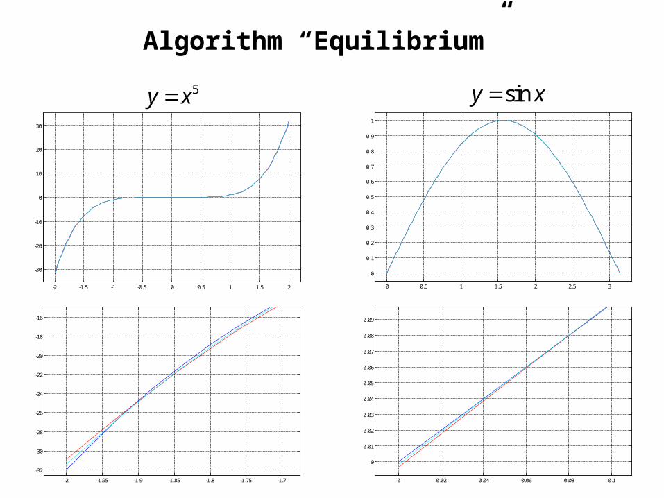
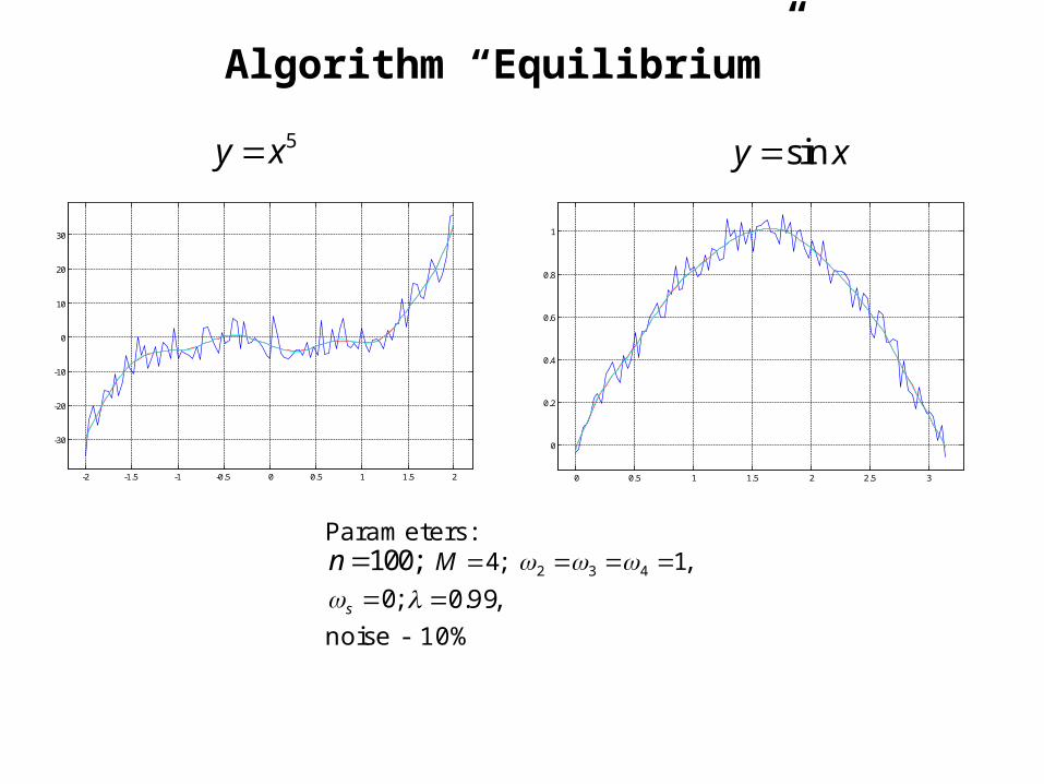
5y x siny x
Algorithm “Equilibrium”
-2 -1.5 -1 -0.5 0 0.5 1 1.5 2
-30
-20
-10
0
10
20
30
0 0.5 1 1.5 2 2.5 3
0
0.2
0.4
0.6
0.8
1
5y x siny x
Parameters: 100;n ;4M ,1432
;0s ,99.0 noise - 10%
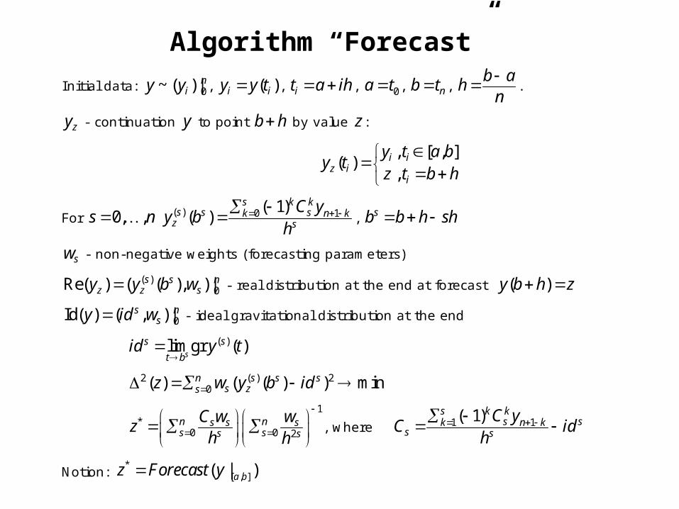
Algorithm “Forecast” Initial data: 0~ ( ) |niy y , ( )i iy y t , it a ih , 0a t , nb t ,
b ah
n .
zy - continuation y to point b h by value z :
, [ , ]( )
,ii
z ii
t a byy t
t b hz
For 0, ,s n ( ) 0 1( 1)( )
s k ks s sk n k
z s
C yy b
h
, sb b h sh
sw - non-negative weights (forecasting parameters)
( )0Re( ) ( ( ), ) |s s n
z z sy y b w - real distribution at the end at forecast ( )y b h z
0Id( ) ( , ) |s nsy id w - ideal gravitational distribution at the end
( )limgr ( )s
ss
t bid y t
( )2 20( ) ( ( ) ) minsn s s
s zsz w y b id
1*
0 0 2n ns s ss ss s
C w wz
h h
, where 1 1( 1)s k k
ssk n ks s
C yC id
h
Notion: *
[ , ]( | )a bz Forecast y
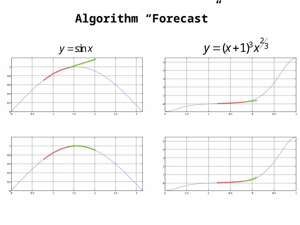
Algorithm “Forecast”
0 0.5 1 1.5 2 2.5 30
0.2
0.4
0.6
0.8
1
0 0.5 1 1.5 2 2.5 30
0.2
0.4
0.6
0.8
1
-2 -1.5 -1 -0.5 0 0.5 1
0
1
2
3
4
5
-2 -1.5 -1 -0.5 0 0.5 1
0
1
2
3
4
5
23 3( 1)y x x siny x
-2 -1.5 -1 -0.5 0 0.5 1-1
0
1
2
3
4
5
6
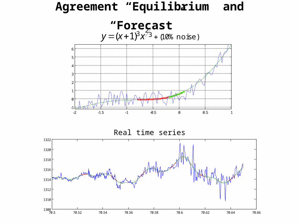
Agreement “Equilibrium” and “Forecast” 23 3 (10% )( 1)y x x noise
70.5 70.52 70.54 70.56 70.58 70.6 70.62 70.64 70.661308
1310
1312
1314
1316
1318
1320
1322
Real time series
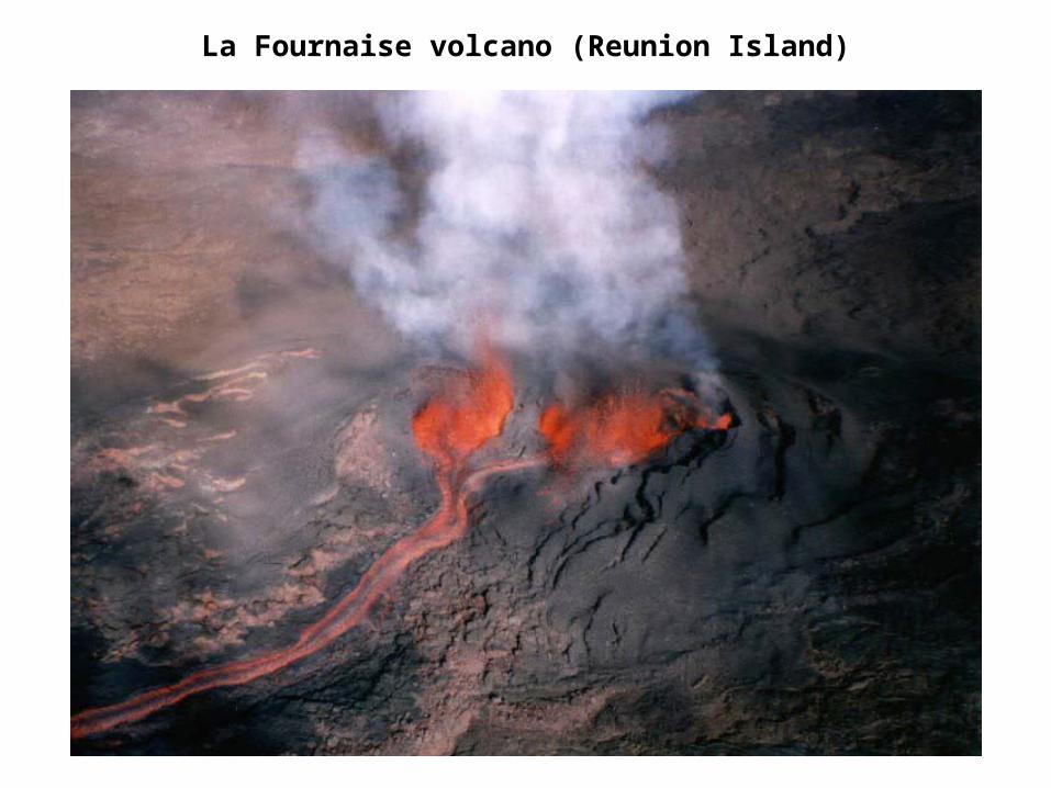
La Fournaise volcano (Reunion Island)
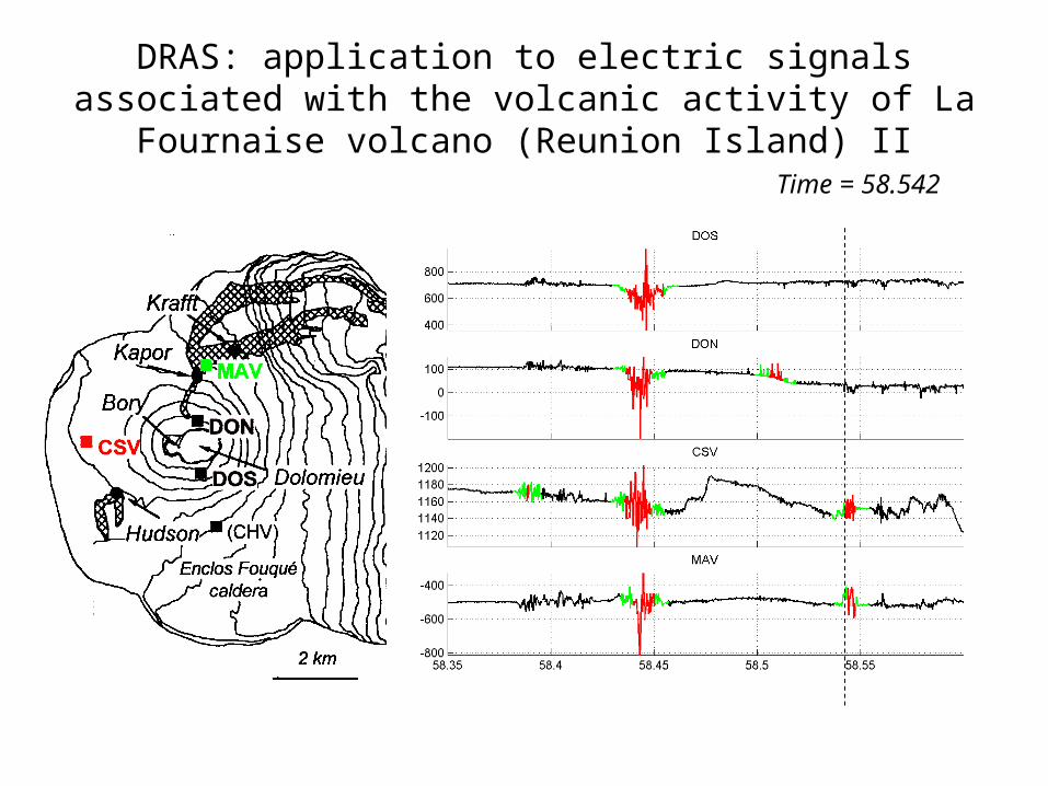
DRAS: application to electric signals associated with the volcanic activity of La Fournaise volcano (Reunion Island) II
Time = 58.542
DRAS and FLARS
Algorithms DRAS (Difference Recognition Algorithm for Signals ) and FLARS (Fuzzy Logic Algorithm for Recognition of Signals) are a results of “smooth” modeling (in fuzzy mathematics sense) of interpreter’s logic, which searches for anomalies at the record.
DRAS and FLARS is really based on fuzzy mathematic principals.
Interpreter’s Logic
Local level:
Interpreter glances at the record and estimates activity of its sufficiently small fragments by positive numbers. At the same time, he puts some numeric marks to the centres of the fragments. In this way, from initial record interpreter necessarily proceeds to a non-negative function. It is naturally to call this function by rectification of the initial time series. Indeed, greater values of this function correspond to more anomalous points (centres of fragments).
Global level:
The anomalies on the record are the uplifts on its rectification.
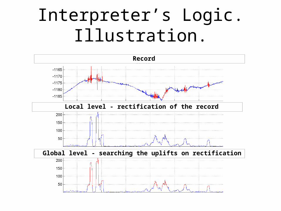
Interpreter’s Logic. Illustration.
Record
Local level - rectification of the record
Global level - searching the uplifts on rectification
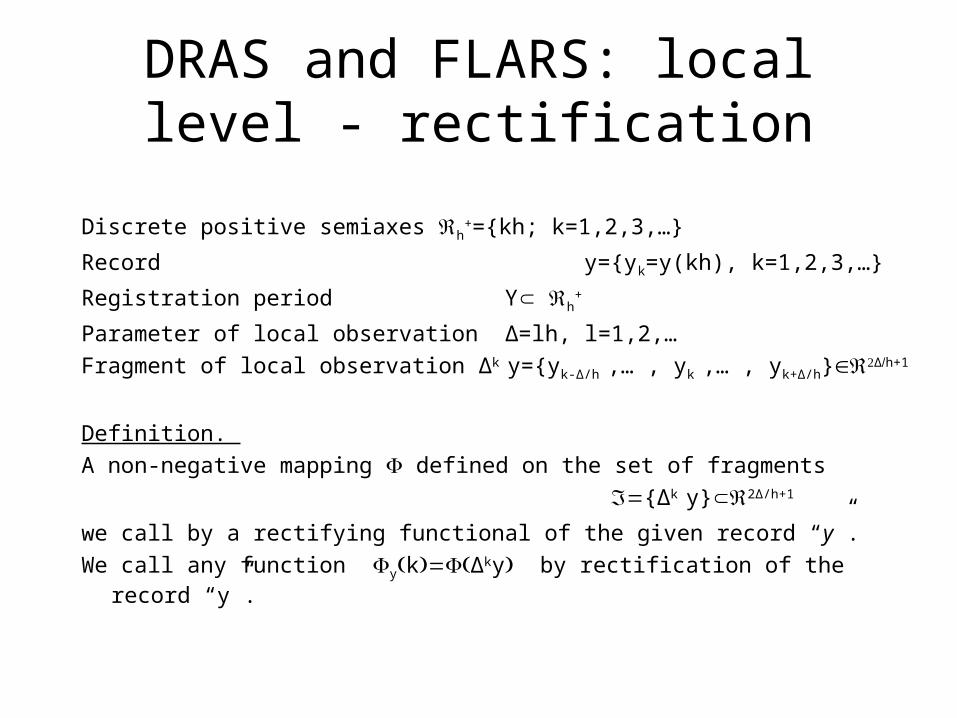
DRAS and FLARS: local level - rectification
Discrete positive semiaxes h+={kh; k=1,2,3,…}
Record y={yk=y(kh), k=1,2,3,…}
Registration period Y h+
Parameter of local observation Δ=lh, l=1,2,…
Fragment of local observation Δk y={yk-Δ/h ,… , yk ,… , yk+Δ/h}Δh+1
Definition.
A non-negative mapping defined on the set of fragments
{Δk y}2Δ/h+1
we call by a rectifying functional of the given record “y”.
We call any function ykΔky by rectification of the record “y”.
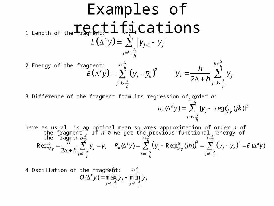
Examples of rectifications1 Length of the fragment:
2 Energy of the fragment:
3 Difference of the fragment from its regression of order n:
here as usual is an optimal mean squares approximation of order n of the fragment . If n=0 we get the previous functional “energy of the fragment”:
4 Oscillation of the fragment:
1
1
kh
kj j
j kh
L y y y
2k
hk
j k
j kh
E y y y
2
kh
k j
j kh
hy y
h
2( ) [ Regr ( )]k
kh
k nn j y
j kh
R y y jk
0Regr2
k
kh
j ky
j kh
hy y
h
2 200 ( ) Regr ( ) ( )k
k kh h
k kj j ky
j k j kh h
R y y jh y y E y
( ) max mink k
h hk
j jj kj k
hh
O y y y
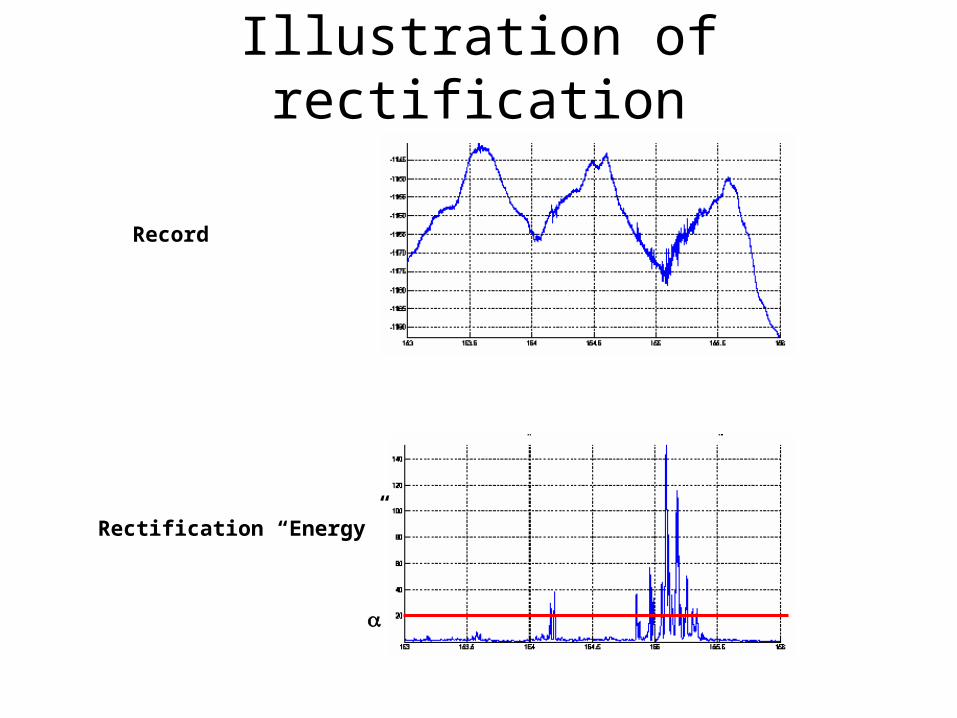
Illustration of rectification
Record
Rectification “Energy”
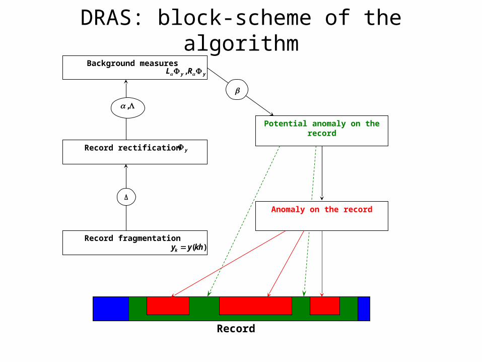
DRAS: block-scheme of the algorithmBackground measures
Record rectification
Record fragmentation
Potential anomaly on the record
Anomaly on the record
,
,y yL R
y
( )ky y kh
Record
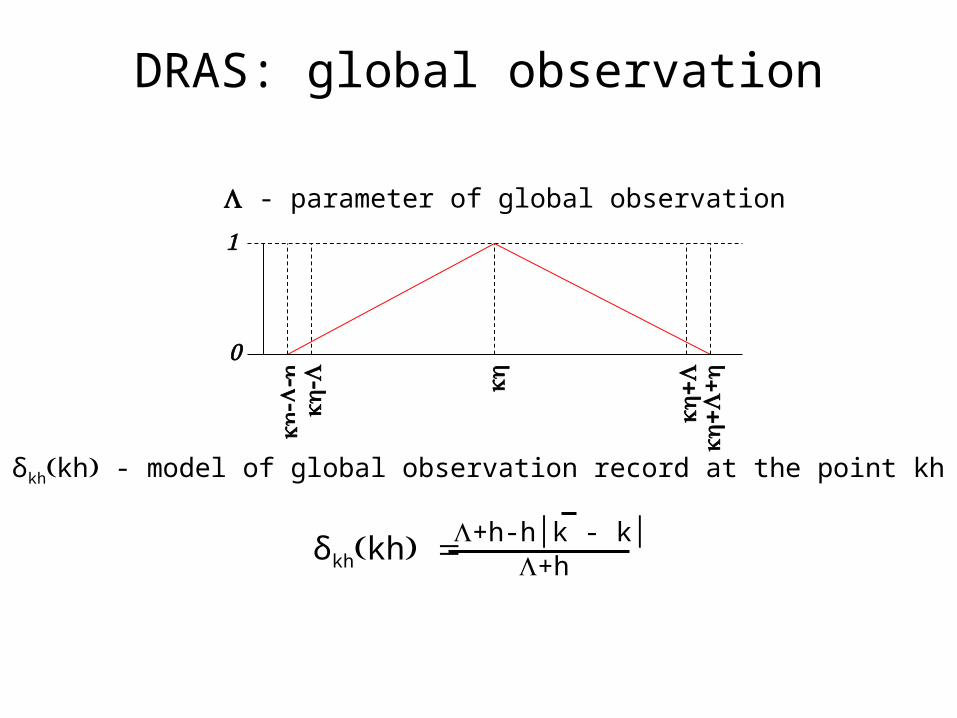
DRAS: global observation
+
- parameter of global observation
δkhkh - model of global observation record at the point kh
δkhkh +h-h│k - k│+h
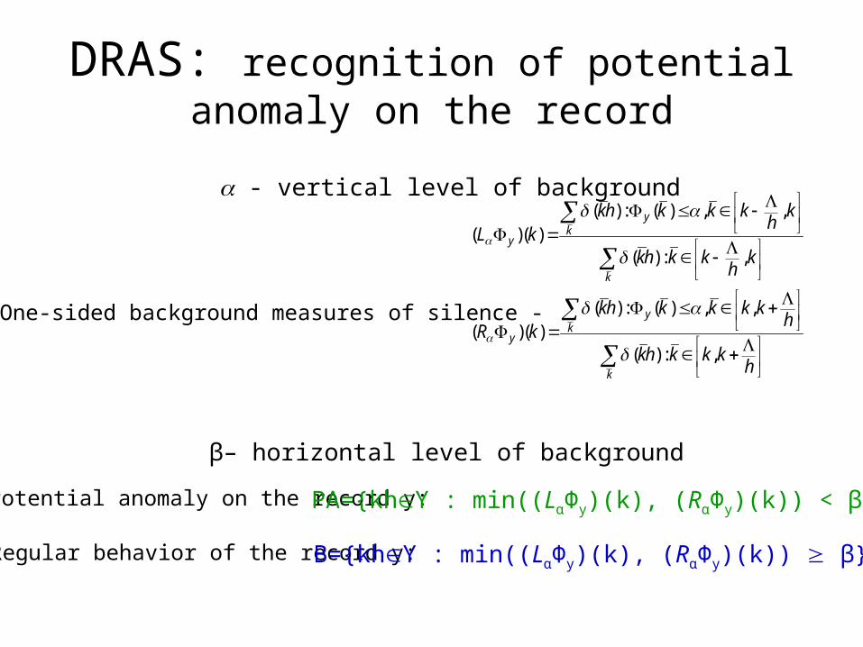
DRAS: recognition of potential anomaly on the record
( ) : ( ) , ,( )( )
( ) : ,
( ) : ( ) , ,( )( )
( ) : ,
yk
y
k
yk
y
k
kh k k k kh
L kkh k k k
h
kh k k k kh
R kkh k k k
h
One-sided background measures of silence -
β– horizontal level of background
Potential anomaly on the record y:
- vertical level of background
PA={khY : min((LαΦy)(k), (RαΦy)(k)) < β}
Regular behavior of the record y: B={khY : min((LαΦy)(k), (RαΦy)(k)) β}
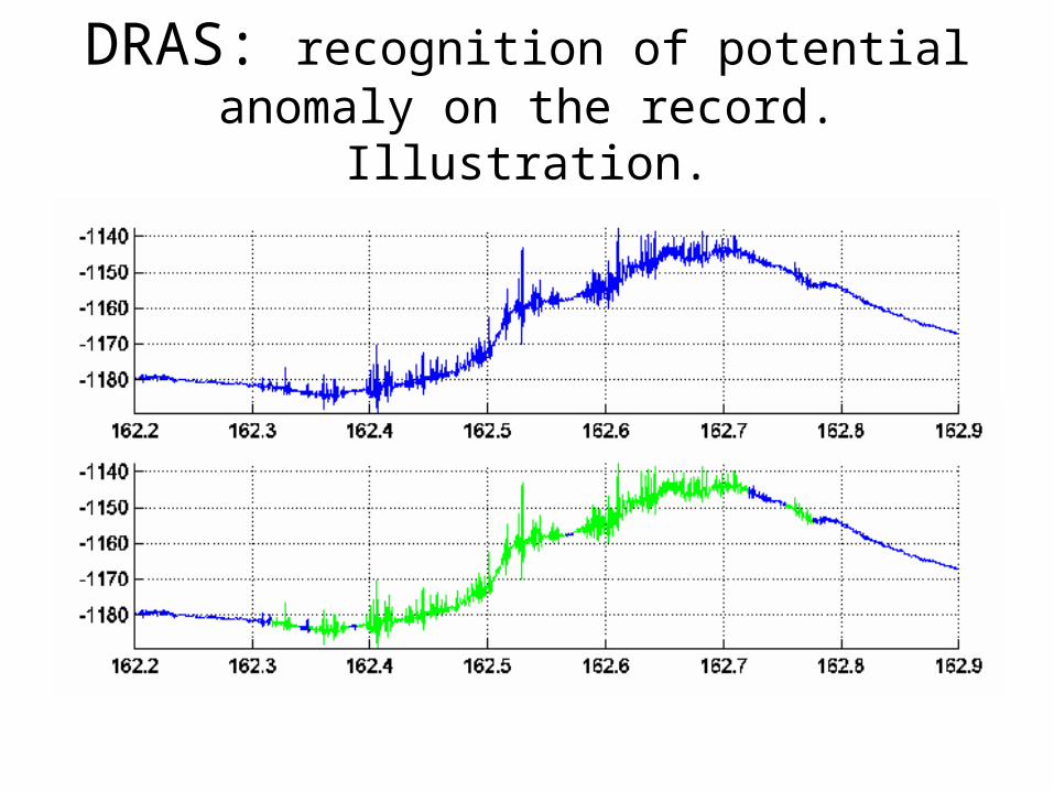
DRAS: recognition of potential anomaly on the record. Illustration.
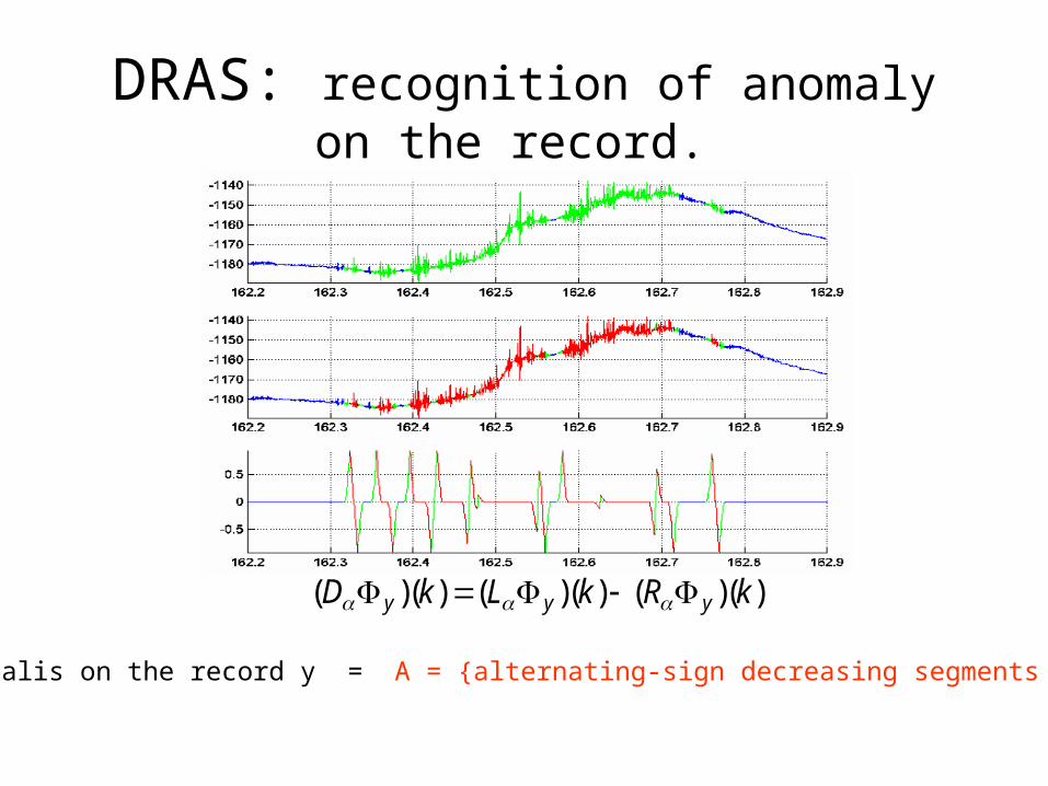
DRAS: recognition of anomaly on the record.
( )( ) ( )( ) ( )( )y y yD k L k R k
Genuine anomalis on the record y = A = {alternating-sign decreasing segments for (DαΦy)(k)}

DRAS: application to electric signals associated with the volcanic activity of La Fournaise volcano (Reunion
Island) I
Station – DON, direction - EW
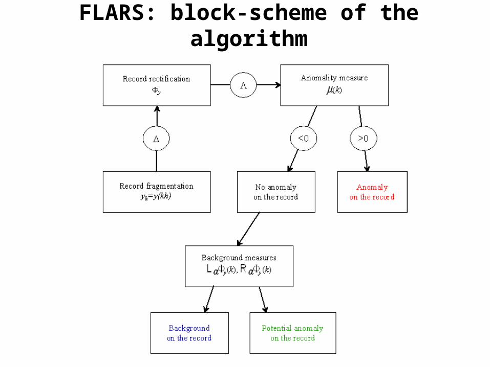
FLARS: block-scheme of the algorithm
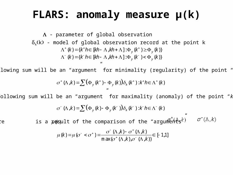
FLARS: anomaly measure μ(k)
- parameter of global observation
δkk - model of global observation record at the point k( ) { [ , ] : ( ) ( )}y yk k h kh kh k k ( ) { [ , ] : ( ) ( )}y yk k h kh kh k k
( , ) ( ) ( ) ( ) : ( )y y kk k k k k h k
( , ) ( ) ( ) ( ) : ( )y y kk k k k k h k
( , ) ( , )( ) ( ) [ 1,1]
max( ( , ), ( , ))
k kk
k k
The following sum will be an “argument” for minimality (regularity) of the point “kh”
The following sum will be an “argument” for maximality (anomaly) of the point “kh”
The measure is a result of the comparison of the “arguments” and( )k
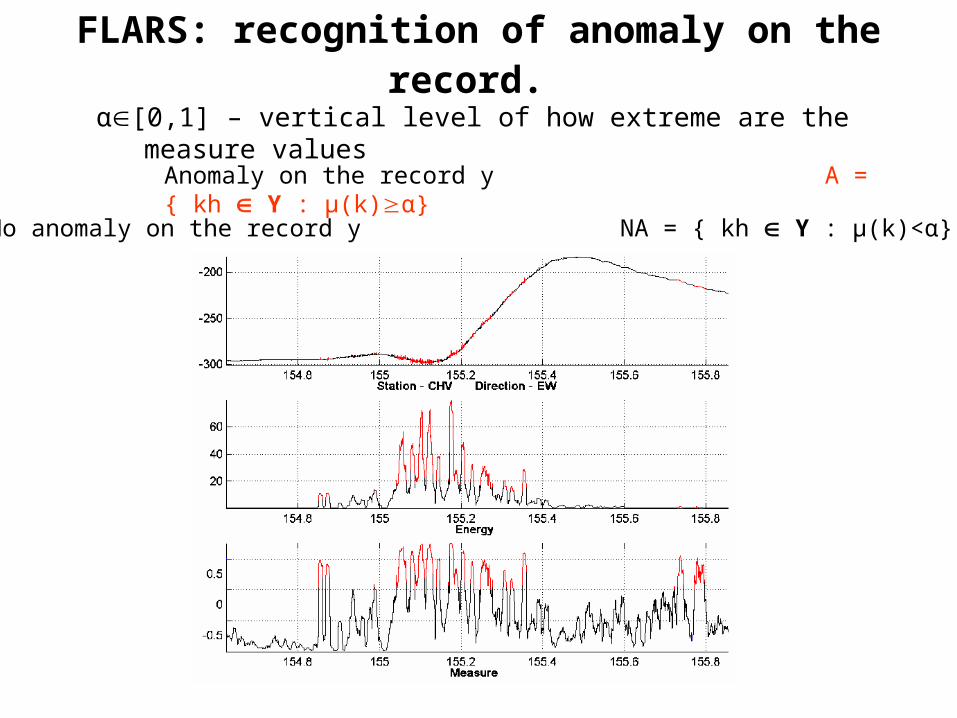
FLARS: recognition of anomaly on the record. α[0,1] – vertical level of how extreme are the measure values
No anomaly on the record y NA = { kh Y : μ(k)<α}
Anomaly on the record y A = { kh Y : μ(k)α}
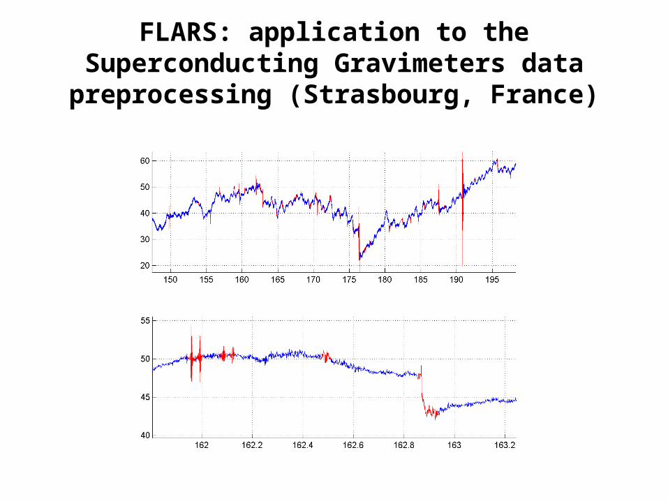
FLARS: application to the Superconducting Gravimeters data preprocessing (Strasbourg,
France)
Construction scheme of DMA
Fussy comparisons onpositive numbers
Nearness in finite metrical space
Limit in finite metrical space
Density as measure oflimitness
Smoothtime series.Equilibrium
Monotonous time series
Fussy logicand geometry on
time series:geometrymeasures
Separation of dense subset.
Crystal. Monolith.
Clasterization.Rodin
Predicationof time series.
Forecast
Anomalies ontime series.
DRAS. FLARS
Extremums on
time series.
Convextime series
Search of linearstructure.Tracing
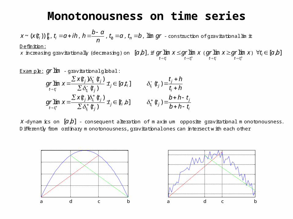
Monotonousness on time series
0~ ( ( )) |nix x t , it a ih , b a
hn , 0t a , nt b , lim gr - construction of gravitational limit
Definition: x increasing gravitationally (decreasing) on [ , ]a b , if lim lim
i it t t tgr x gr x
( lim lim
i it t t tgr x gr x
) [ , ]it a b
Example: limgr - gravitational global :
( ) ( )lim : [ , ]
( )i
i i
j t jj i
t t t j
x t tgr x t a t
t
( )
i
jt j
i
t ht
t h
,( ) ( )
lim : [ ]( )
i
i i
j t jj i
t t t j
bx t t
gr x t tt
( )
i
jt j
i
b h tt
b h t
x -dynamics on [ , ]a b - consequent alteration of maximum opposite gravitational monotonousness. Differently from ordinary monotonousness, gravitational ones can intersect with each other
a d c b a d c b
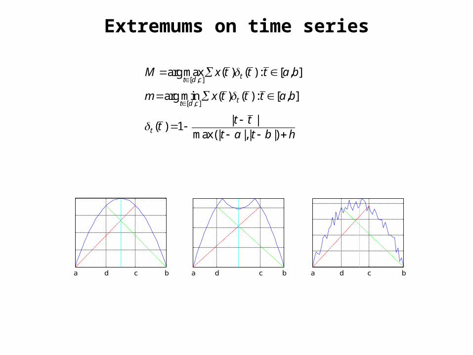
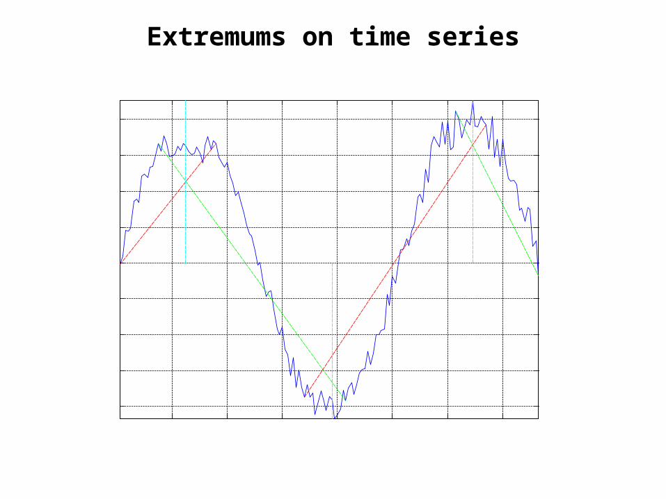
Extremums on time series
[ , ]arg max ( ) ( ) : [ , ]tt d c
M x t t t a b
[ , ]arg min ( ) ( ) : [ , ]tt d c
m x t t t a b
| |( ) 1
max(| |,| |)tt t
tt a t b h
a d c b a d c b a d c b
Extremums on time series
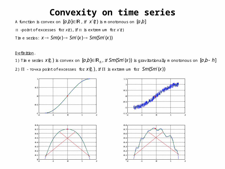
Convexity on time seriesA function is convex on [ , ]a b , if ( )x t is monotonous on [ , ]a b
-point of excesses for ( )x t , if is extremum for ( )x t
Time serios: ( ) ( ) ( ( ))x Sm x Sm x Sm Sm x
Definition.
1) Time series ( )ix t is convex on [ , ] ha b , if ( ( ))Sm Sm x is gravitationally monotonous on [ , ]a b h
2) - точка point of excesses for ( )ix t , if is extremum for ( ( ))Sm Sm x
-2 -1 0 1 2-1
-0.5
0
0.5
1
-2 -1 0 1 20
0.1
0.2
0.3
0.4
0.5
0.6
0.7
0.8
-2 -1 0 1 2-1.5
-1
-0.5
0
0.5
1
1.5
-2 -1 0 1 20
0.1
0.2
0.3
0.4
0.5
0.6
0.7
0.8

Construction scheme of DMA
Fussy comparisons onpositive numbers
Nearness in finite metrical space
Limit in finite metrical space
Density as measure oflimitness
Smoothtime series.Equilibrium
Monotonous time series
Fussy logicand geometry on
time series:geometrymeasures
Separation of dense subset.
Crystal. Monolith.
Clasterization.Rodin
Predicationof time series.
Forecast
Anomalies ontime series.
DRAS. FLARS
Extremums on
time series.
Convextime series
Search of linearstructure.Tracing
Elementary measures
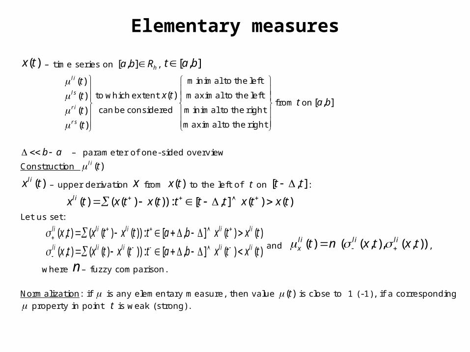
( )x t – time series on [ , ] ha b R , [ , ]t a b
( )
( )( )[ , ]
( )
( )
l i
l s
r i
r s
t
x ttt a b
t
t
minimal to the left
to which extent maximal to the leftfrom on
canbe considered minimal to the right
maximal to the right
b a – parameter of one-sided overview
Construction ( )l i t
( )lix t – upper derivation x from ( )x t to the left of t on [ , ]t t :
( ) ( ( ) ( )) : [ , ] ( ) ( )lix t x t x t t t t x t x t
Let us set:
( , ) ( ( ) ( )) : [ , ] ( ) ( )
( , ) ( ( ) ( )) : [ , ] ( ) ( )
li li li li li
li li li li li
x t x t x t t a b x t x t
x t x t x t t a b x t x t
and ( ) ( ( , ), ( , ))li li li
x t n x t x t ,
where n – fuzzy comparison. Normalization: if is any elementary measure, then value ( )t is close to 1 (-1), if a corresponding property in point t is weak (strong).
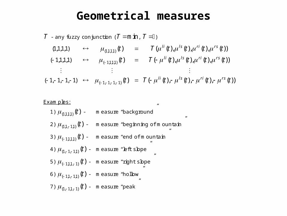
Geometrical measures
T - any fuzzy conjunction ( minT , T )
(1,1,1,1)
( 1,1,1,1)
( 1, 1, 1, 1)
(1,1,1,1)
( 1,1,1,1)
( 1, 1, 1, 1)
( ) ( ( ), ( ), ( ), ( ))
( ) ( ( ), ( ), ( ), ( ))
( ) ( ( ), ( ), ( ), ( ))
li l s ri rs
li l s ri rs
li l s ri rs
t T t t t t
t T t t t t
t T t t t t
Examples:
1) (1,1,1,1)( )t - measure “background”
2) (1,1, 1,1)( )t - measure “beginning of mountain”
3) ( 1,1,1,1)( )t - measure “end of mountain”
4) (1, 1, 1,1)( )t - measure “left slope”
5) ( 1,1,1, 1)( )t - measure “right slope”
6) ( 1,1, 1,1)( )t - measure “hollow”
7) (1, 1,1, 1)( )t - measure “peak”
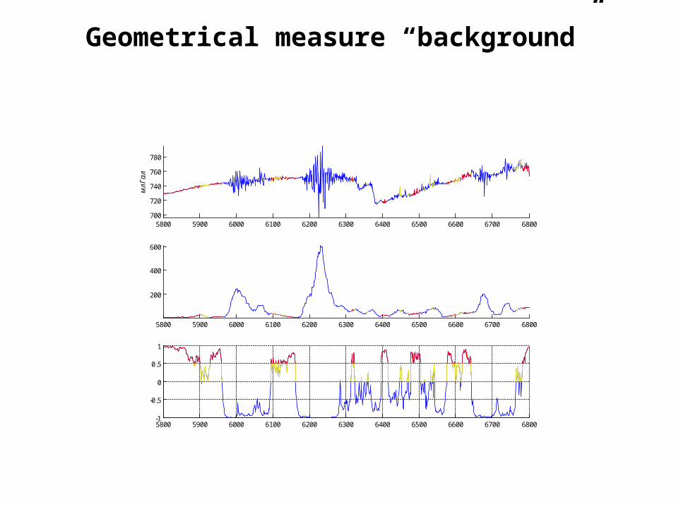
Geometrical measure “background”
5800 5900 6000 6100 6200 6300 6400 6500 6600 6700 6800700
720
740
760
780
мл
Га
л
5800 5900 6000 6100 6200 6300 6400 6500 6600 6700 6800
200
400
600
5800 5900 6000 6100 6200 6300 6400 6500 6600 6700 6800-1
-0.5
0
0.5
1
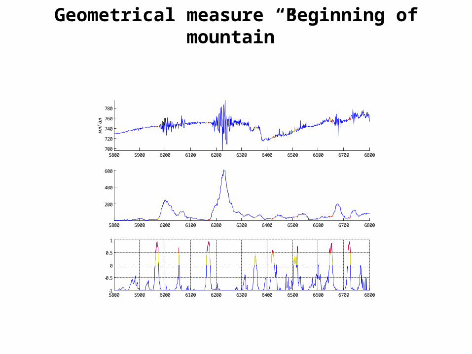
Geometrical measure “Beginning of mountain”
5800 5900 6000 6100 6200 6300 6400 6500 6600 6700 6800700
720
740
760
780
мл
Га
л
5800 5900 6000 6100 6200 6300 6400 6500 6600 6700 6800
200
400
600
5800 5900 6000 6100 6200 6300 6400 6500 6600 6700 6800-1
-0.5
0
0.5
1
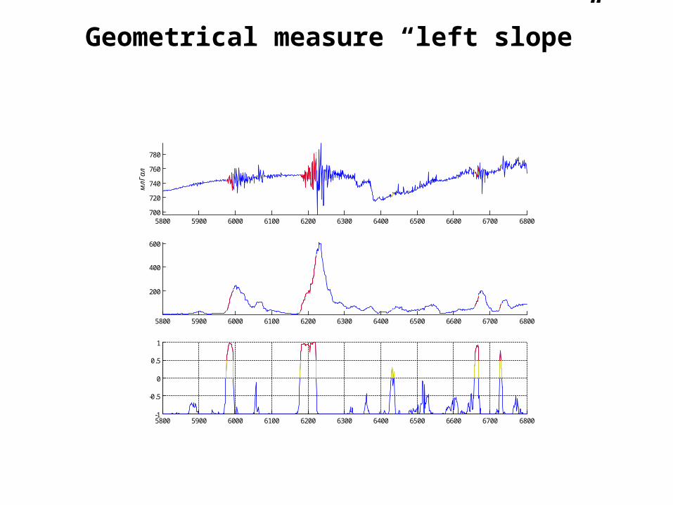
Geometrical measure “left slope”
5800 5900 6000 6100 6200 6300 6400 6500 6600 6700 6800700
720
740
760
780
мл
Га
л
5800 5900 6000 6100 6200 6300 6400 6500 6600 6700 6800
200
400
600
5800 5900 6000 6100 6200 6300 6400 6500 6600 6700 6800-1
-0.5
0
0.5
1
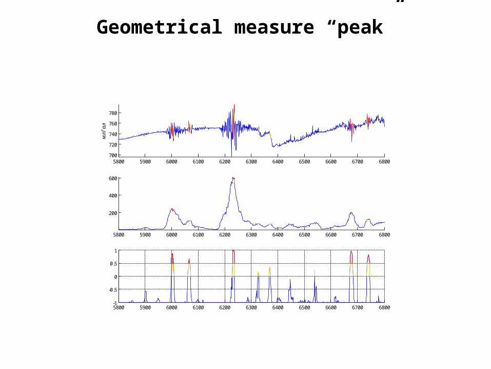
Geometrical measure “peak”
5800 5900 6000 6100 6200 6300 6400 6500 6600 6700 6800700
720
740
760
780
мл
Га
л
5800 5900 6000 6100 6200 6300 6400 6500 6600 6700 6800
200
400
600
5800 5900 6000 6100 6200 6300 6400 6500 6600 6700 6800-1
-0.5
0
0.5
1

Thank you