Discrete Gaussian Leftover Hash Lemma overInfinite Domains

Shweta Agrawal1, Craig Gentry2, Shai Halevi2, and Amit Sahai1

1 UCLA2 IBM Research

Abstract. The classic Leftover Hash Lemma (LHL) is often used toargue that certain distributions arising from modular subset-sums areclose to uniform over their finite domain. Though very powerful, theapplicability of the leftover hash lemma to lattice based cryptography islimited for two reasons. First, typically the distributions we care about inlattice-based cryptography are discrete Gaussians, not uniform. Second,the elements chosen from these discrete Gaussian distributions lie in aninfinite domain: a lattice rather than a finite field.In this work we prove a “lattice world” analog of LHL over infinitedomains, proving that certain “generalized subset sum” distributionsare statistically close to well behaved discrete Gaussian distributions,even without any modular reduction. Specifically, given many vectorsximi=1 from some lattice L ⊂ Rn, we analyze the probability distribu-tion

∑mi=1 zixi where the integer vector z ∈ Zm is chosen from a discrete

Gaussian distribution. We show that when the xi’s are “random enough”and the Gaussian from which the z’s are chosen is “wide enough”, thenthe resulting distribution is statistically close to a near-spherical dis-crete Gaussian over the lattice L. Beyond being interesting in its ownright, this “lattice-world” analog of LHL has applications for the newconstruction of multilinear maps [5], where it is used to sample DiscreteGaussians obliviously. Specifically, given encoding of the xi’s, it is usedto produce an encoding of a near-spherical Gaussian distribution overthe lattice. We believe that our new lemma will have other applications,and sketch some plausible ones in this work.

1 Introduction

The Leftover Hash Lemma (LHL) is a central tool in computer science, statingthat universal hash functions are good randomness extractors. In a characteristicapplication, the universal hash function may often be instantiated by a simpleinner product function, where it is used to argue that a random linear combina-tion of some elements (that are chosen at random and then fixed “once and forall”) is statistically close to the uniform distribution over some finite domain.Though extremely useful and powerful in general, the applicability of the left-over hash lemma to lattice based cryptography is limited for two reasons. First,typically the distributions we care about in lattice-based cryptography are dis-crete Gaussians, not uniform. Second, the elements chosen from these discrete

Gaussian distributions lie in an infinite domain: a lattice rather than a finitefield.

The study of discrete Gaussian distributions underlies much of the advancesin lattice-based cryptography over the last decade. A discrete Gaussian distri-bution is a distribution over some fixed lattice, in which every lattice point issampled with probability proportional to its probability mass under a standard(n-dimensional) Gaussian distribution. Micciancio and Regev have shown in [10]that these distributions share many of the nice properties of their continuouscounterparts, and demonstrated their usefulness for lattice-based cryptography.Since then, discrete Gaussian distributions have been used extensively in allaspects of lattice-based cryptography (most notably in the famous “Learningwith Errors” problem and its variants [14]). Despite their utility, we still do notunderstand discrete Gaussian distributions as well as we do their continuouscounterparts.

A Gaussian Leftover Hash Lemma for Lattices?

The LHL has been applied often in lattice-based cryptography, but sometimesawkwardly. As an example, in the integer-based fully homomorphic encryptionscheme of van Dijk et al. [18], ciphertexts live in the lattice Z. Roughly speaking,the public key of that scheme contains many encryptions of zero, and encryptionis done by adding the plaintext value to a subset-sum of these encryptions ofzero. To prove security of this encryption method, van Dijk et al. apply theleft-over hash lemma in this setting, but with the cost of complicating theirencryption procedure by reducing the subset-sum of ciphertexts modulo a singlelarge ciphertext, so as to bring the scheme back in to the realm of finite ringswhere the leftover hash lemma is naturally applied.3 It is natural to ask whetherthat scheme remains secure also without this artificial modular reduction, andmore generally whether there is a more direct way to apply the LHL in settingswith infinite rings.

As another example, in the recent construction of multilinear maps [5], Garget. al. require a procedure to randomize “encodings” to break simple algebraicrelations that exist between them. One natural way to achieve this randomizationis by adding many random encodings of zero to the public parameters, andadding a random linear combination of these to re-randomize a given encoding(without changing the encoded value). However, in their setting, there is noway to “reduce” the encodings so that the LHL can be applied. Can they arguethat the new randomized encoding yields an element from some well behaveddistribution?

In this work we prove an analog of the leftover hash lemma over lattices,yielding a positive answers to the questions above. We use discrete Gaussiandistributions as our notion of “well behaved” distributions. Then, for m vectorsxii∈[m] chosen “once and for all” from an n dimensional lattice L ⊂ Rn,

3 Once in the realms of finite rings, one can alternatively use the generic proof ofRothblum [15], which also uses the LHL.

and a coefficient vector z chosen from a discrete Gaussian distribution over theintegers, we give sufficient conditions under which the distribution

∑mi=1 zixi is

“well behaved.”

Oblivious Gaussian Sampler

Another application of our work is in the construction of an extremely simplediscrete Gaussian sampler [6, 13]. Such samplers, that sample from a sphericaldiscrete Gaussian distribution over a lattice have been constructed by [6] (usingan algorithm by Klein [7]) as well as Peikert [13]. Here we consider a much sim-pler discrete Gaussian sampler (albeit a somewhat imperfect one). Specifically,consider the following sampler. In an offline phase, for m > n, the sampler sam-ples a set of short vectors x1,x2, . . . ,xm from L – e.g., using GPV or Peikert’salgorithm. Then, in the online phase, the sampler generates z ∈ Zm according toa discrete Gaussian and simply outputs

∑mi=1 zixi. But does this simpler sam-

pler work – i.e., can we say anything about its output distribution? Also, howsmall can we make the dimension m of z and how small can we make the entriesof z? Ideally m would be not much larger than the dimension of the lattice andthe entries of z have small variance – e.g., O(

√n).

A very useful property of such a sampler is that it can be made oblivious toan explicit representation of the underlying lattice, which makes it applicableeasily within an additively homomorphic scheme. Namely, if you are given latticepoints encrypted under an additively homomorphic encryption scheme, you canuse them to generate an encrypted well behaved Gaussian on the underlyinglattice. Previous samplers [6, 13] are too complicated to use within an additivelyhomomorphic encryption scheme 4.

Our Results

In this work, we obtain a discrete Gaussian version of the LHL over infiniterings. Formally, consider an n dimensional lattice L and (column) vectors X =[x1|x2| . . . |xm] ∈ L. We choose xi according to a discrete Gaussian distribution

DL,S , where DL,S is defined as DL,S,c(x) =ρS,c(x)ρS,c(L)

with ρS,c(x)def= exp(−π‖x−

c‖2/s2) and ρS,c(A) for set A denotes∑x∈A ρS,c(x).

Let z ← DZm,s′ , we analyze the conditions under which the vector X · z isstatistically close to a “near-spherical” discrete Gaussian. Formally, consider:

EX,s′def= X · z : z ← DZm,s′

Then, we prove that EX,s′ is close to a discrete Gaussian over L of moder-ate “width”. Specifically, we show that for large enough s′, with overwhelmingprobability over the choice of X:

4 As noted by Peikert [13], one can generate an ellipsoidal Gaussian distribution overthe lattice given a basis B by just outputting y ← B · z where z is a discreteGaussian, but this ellipsoidal Gaussian distribution would typically be very skewed.

1. EX,s′ is statistically close to the ellipsoid Gaussian DL,s′X> , over L.2. The singular values of the matrix X are of size roughly s

√m, hence the

shape of DL,s′X> is “roughly spherical”. Moreover, the “width” of DL,s′X>is roughly s′s

√m = poly(n).

We emphasize that it is straightforward to show that the covariance matrixof EX,s′ is exactly s′

2XX>. However, the technical challenge lies in showing

that EX,s′ is close to a discrete Gaussian for a non-square X. Also note thatfor a square X, the shape of the covariance matrix XX> will typically be very“skewed” (i.e., the least singular value of X> is typically much smaller than thelargest singular value). We note that the “approximately spherical” nature of theoutput distribution is important for performance reasons in applications such asGGH: These applications must choose parameters so that the least singular valueof X “drowns out” vectors of a certain size, and the resulting vectors that theydraw from EX,s′ grow in size with the largest singular value of X, hence it isimportant that these two values be as close as possible.

Our Techniques

Our main result can be argued along the following broad outline. Our first theo-rem (Theorem 2) says that the distribution of X ·z ← EX,s′ is indeed statisticallyclose to a discrete Gaussian over L, as long as s′ exceeds the smoothing param-eter of a certain “orthogonal lattice” related to X (denoted A). Next, Theorem3 clarifies that A will have a small smoothing parameter as long as X> is “reg-ularly shaped” in a certain sense. Finally, we argue in Lemma 8 that when thecolumns of X are chosen from a discrete Gaussian, xi ← DL,S , then X> is“regularly shaped,” i.e. has singular values all close to σn(S)

√m.

The analysis of the smoothing parameter of the “orthogonal lattice” A isparticularly challenging and requires careful analysis of a certain “dual lattice”related to A. Specifically, we proceed by first embedding A into a full rank latticeAq and then move to study Mq – the (scaled) dual of Aq. Here we obtain a lowerbound on λn+1(Mq), i.e. the n + 1th minima of Mq. Next, we use a theoremby Banasczcyk to convert the lower bound on λn+1(Mq) to an upper boundon λm−n(Aq), obtaining m − n linearly independent, bounded vectors in Aq.We argue that these vectors belong to A, thus obtaining an upper bound onλm−n(A). Relating λm−n(A) to ηε(A) using a lemma by Micciancio and Regevcompletes the analysis. (We note that probabilistic bounds on the minima andsmoothing parameter Aq,Mq are well known in the case when the entries ofmatrix X are uniformly random mod q (e.g. [6]), but here we obtain bounds inthe case when X has Gaussian entries significantly smaller than q.)

To argue that X> is regularly shaped, we begin with the literature of randommatrices which establishes that for a matrix H ∈ Rm×n, where each entry of His distributed as N (0, s2) and m is sufficiently greater than n, the singular valuesof H are all of size roughly s

√m. We extend this result to discrete Gaussians –

showing that as long as each vector xi ← DL,S where S is “not too small” and“not too skewed”, then with high probability the singular values of X> are allof size roughly s

√m.

Related Work

Properties of linear combinations of discrete Gaussians have been studied beforein some cases by Peikert [13] as well as more recently by Boneh and Freeman [3].Peikert’s “convolution lemma” (Theorem 3.1 in [13]) analyzes certain cases inwhich a linear combination of discrete Gaussians yields a discrete Gaussian, inthe one dimensional case. More recently, Boneh and Freeman [3] observed thatunder certain conditions, a linear combination of discrete Gaussians over a latticeis also a discrete Gaussian. However, the deviation of the Gaussian needed toachieve this are quite large. Related questions were considered by Lyubashevsky[9] where he computes the expectation of the inner product of discrete Gaussians.

Discrete Gaussian samplers have been studied by [6] (who use an algorithmby [7]) and [13]. These works describe a discrete Gaussian sampling algorithmthat takes as input a ‘high quality’ basis B for an n dimensional lattice L andoutput a sample from DL,s,c. In [6], s ≥ ‖B‖ · ω(

√log n), and B = maxi ‖bi‖

is the Gram Schmidt orthogonalization of B. In contrast, the algorithm of [13]requires s ≥ σ1(B), i.e. the largest singular value of B, but is fully parallelizable.Both these samplers take as input an explicit description of a “high quality basis”of the relevant lattice, and the quality of their output distribution is related tothe quality of the input basis.

Peikert’s sampler [13] is elegant and its complexity is difficult to beat: theonly online computation is to compute c−B1bB−11 (c−x2)e, where c is the centerof the Gaussian, B1 is the sampler’s basis for its lattice L, and x2 is a vectorthat is generated in an offline phase (freshly for each sampling) in a way designedto “cancel” the covariance of B1 so as to induce a purely spherical Gaussian.However, since our sampler just directly takes an integer linear combination oflattice vectors, and does not require extra precision for handling the inverse B−11 ,it might outperform Peikert’s in some situations, at least when c = 0.

2 Preliminaries

We say that a function f : R+ → R+ is negligible (and write f(λ) < negl(λ)) iffor every d we have f(λ) < 1/λd for sufficiently large λ. For two distributionsD1 and D2 over some set Ω the statistical distance SD(D1,D2) is

SD(D1,D2)def=

1

2

∑x∈Ω

∣∣PrD1

[x]− PrD2

[x]∣∣

Two distribution ensembles D1(λ) and D2(λ) are statistically close or statisti-cally indistinguishable if SD

(D1(λ),D2(λ)

)is a negligible function of λ.

2.1 Gaussian Distributions

For any real s > 0 and vector c ∈ Rn, define the (spherical) Gaussian func-tion on Rn centered at c with parameter s as ρs,c(x) = exp(−π‖x − c‖2/s2)

for all x ∈ Rn. The normal distribution with mean µ and deviation σ, de-noted N (µ, σ2), assigns to each real number x ∈ R the probability densityf(x) = 1

σ√2π· ρσ√2π,µ(x). The n-dimensional (spherical) continuous Gaussian

distribution with center c and uniform deviation σ2, denoted Nn(c, σ2), justchooses each entry of a dimension-n vector independently from N (ci, σ

2).The n-dimensional spherical Gaussian function generalizes naturally to el-

lipsoid Gaussians, where the different coordinates are jointly Gaussian but areneither identical nor independent. In this case we replace the single varianceparameter s2 ∈ R by the covariance matrix Σ ∈ Rn×n (which must be positive-definite and symmetric). To maintain consistency of notations between the spher-ical and ellipsoid cases, below we let S be a matrix such that S>×S = Σ. Sucha matrix S always exists for a symmetric Σ, but it is not unique. (In fact thereexist such S’es that are not even n-by-n matrices, below we often work with suchrectangular S’es.)

For a rank-n matrix S ∈ Rm×n and a vector c ∈ Rn, the ellipsoid Gaussianfunction on Rn centered at c with parameter S is defined by

ρS,c(x) = exp(− π(x− c)>(S>S)−1(x− c)

)∀x ∈ Rn.

Obviously this function only depends on Σ = S>S and not on the particularchoice of S. It is also clear that the spherical case can be obtained by settingS = sIn, with In the n-by-n identity matrix. Below we use the shorthand ρs(·)(or ρS(·)) when the center of the distribution is 0.

2.2 Matrices and Singular Values

In this note we often use properties of rectangular (non-square) matrices. Form ≥ n and a rank-n matrix5 X ′ ∈ Rm×n, the pseudoinverse of X ′ is the (unique)

m-by-n matrix Y ′ such that X ′>Y ′ = Y ′

>X ′ = In and the columns of Y ′ span

the same linear space as those of X ′. It is easy to see that Y ′ can be expressedas Y ′ = X ′(X ′

>X ′)−1 (note that X ′

>X ′ is invertible since X ′ has rank n).

For a rank-n matrix X ′ ∈ Rm×n, denote UX′ = ‖X ′u‖ : u ∈ Rn, ‖u‖ = 1.The least singular value of X ′ is then defined as σn(X ′) = inf(U ′X) and similarlythe largest singular value of X ′ is σ1(X ′) = sup(U ′X). Some properties of singularvalues that we use later in the text are stated in Fact 1.

Fact 1 For rank-n matrices X ′, Y ′ ∈ Rm×n with m ≥ n, the following holds:

1. If X ′>X ′ = Y ′

>Y ′ then X ′, Y ′ have the same singular values.

2. If Y ′ is the (pseudo)inverse of X ′ then the singular values of X ′, Y ′ arereciprocals.

3. If X ′ is a square matrix (i.e., m = n) then X ′, X ′>

have the same singularvalues.

5 We use the notation X ′ instead of X to avoid confusion later in the text where wewill instantiate X ′ = X>

4. If σ1(Y ′) ≤ δσn(X ′) for some constant δ < 1, then σ1(X ′+Y ′) ∈ [1− δ, 1 +δ]σ1(X ′) and σn(X ′ + Y ′) ∈ [1− δ, 1 + δ]σn(X ′). ut

It is well known that when m is sufficiently larger than n, then the singularvalues of a “random matrix” X ′ ∈ Rm×n are all of size roughly

√m. For example,

Lemma 1 below is a special case of [8, Thm 3.1], and Lemma 2 can be provedalong the same lines of (but much simpler than) the proof of [17, Corollary 2.3.5].

Lemma 1. There exists a universal constant C > 1 such that for any m >2n, if the entries of X ′ ∈ Rm×n are drawn independently from N (0, 1) thenPr[σn(X ′) <

√m/C] < exp(−O(m)). ut

Lemma 2. There exists a universal constant C > 1 such that for any m >2n, if the entries of X ′ ∈ Rm×n are drawn independently from N (0, 1) thenPr[σ1(X ′) > C

√m] < exp(−O(m)). ut

Corollary 1. There exists a universal constant C > 1 such that for any m > 2nand s > 0, if the entries of X ′ ∈ Rm×n are drawn independently from N (0, s2)then

Pr[s√m/C < σn(X ′) ≤ σ1(X ′) < sC

√m]> 1− exp(−O(m)). ut

Remark. The literature on random matrices is mostly focused on analyzing the“hard cases” of more general distributions and m which is very close to n (e.g.,m = (1 + o(1))n or even m = n). For our purposes, however, we only need the“easy case” where all the distributions are Gaussian and m n (e.g., m = n2),in which case all the proofs are much easier (and the universal constant fromCorollary 1 gets closer to one).

2.3 Lattices and their Dual

A lattice L ⊂ Rn is an additive discrete sub-group of Rn. We denote by span(L)the linear subspace of Rn, spanned by the points in L. The rank of L ⊂ Rn isthe dimension of span(L), and we say that L has full rank if its rank is n. Inthis work we often consider lattices of less than full rank.

Every (nontrivial) lattice has bases: a basis for a rank-k lattice L is a set of k

linearly independent points b1, . . . , bk ∈ L such that L = ∑ki=1 zibi : zi ∈ Z ∀i.

If we arrange the vectors bi as the columns of a matrix B ∈ Rn×k then we canwrite L = Bz : z ∈ Zk. If B is a basis for L then we say that B spans L.

Definition 1 (Dual of a Lattice). For a lattice L ⊂ Rn, its dual latticeconsists of all the points in span(L) that are orthogonal to L modulo one, namely:

L∗ = y ∈ span(L) : ∀x ∈ L, 〈x,y〉 ∈ Z

Clearly, if L is spanned by the columns of some rank-k matrix X ∈ Rn×k thenL∗ is spanned by the columns of the pseudoinverse of X. It follows from thedefinition that for two lattices L ⊆M we have M∗ ∩ span(L) ⊆ L∗.

Banasczcyk provided strong transference theorems that relate the size ofshort vectors in L to the size of short vectors in L∗. Recall that λi(L) denotes thei-th minimum of L (i.e., the smallest s such that L contains i linearly independentvectors of size at most s).

Theorem 1 (Banasczcyk [2]). For any rank-n lattice L ⊂ Rm, and for alli ∈ [n],

1 ≤ λi(L) · λn−i+1(L∗) ≤ n.

2.4 Gaussian Distributions over Lattices

The ellipsoid discrete Gaussian distribution over lattice L with parameter S,centered around c, is

∀ x ∈ L,DL,S,c(x) =ρS,c(x)

ρS,c(L),

where ρS,c(A) for set A denotes∑x∈A ρS,c(x). In other words, the probability

DL,S,c(x) is simply proportional to ρS,c(x), the denominator being a normaliza-tion factor. The same definitions apply to the spherical case, which is denoted byDL,s,c(·) (with lowercase s). As before, when c = 0 we use the shorthand DL,S(or DL,s). The following useful fact that follows directly from the definition,relates the ellipsoid Gaussian distributions over different lattices:

Fact 2 Let L ⊂ Rn be a full-rank lattice, c ∈ Rn a vector, and S ∈ Rm×n,B ∈ Rn×n two rank-n matrices, and denote L′ = B−1v : v ∈ L, c′ = B−1c,and S′ = S×(B>)−1. Then the distribution DL,S,c is identical to the distributioninduced by drawing a vector v ← DL′,S′,c′ and outputting u = Bv. ut

A useful special case of Fact 2 is when L′ is the integer lattice, L′ = Zn,in which case L is just the lattice spanned by the basis B. In other words, theellipsoid Gaussian distribution on L(B), v ← DL(B),S,c, is induced by drawingan integer vector according to z ← DZn,S′,c′ and outputting v = Bz, where

S′ = S(B−1)> and c′ = B−1c.Another useful special case is where S = sB>, so S is a square matrix

and S′ = sIn. In this case the ellipsoid Gaussian distribution v ← DL,S,c isinduced by drawing a vector according to the spherical Gaussian u ← DL′,s,c′and outputting v = 1

sS>u, where c′ = s(S>)−1c and L′ = s(S>)−1v : v ∈ L.

Smoothing parameter. As in [10], for lattice L and real ε > 0, the smoothingparameter of L, denoted ηε(L), is defined as the smallest s such that ρ1/s(L

∗ \0) ≤ ε. Intuitively, for a small enough ε, the number ηε(L) is sufficiently largerthan L’s fundamental parallelepiped so that sampling from the correspondingGaussian “wipes out the internal structure” of L. Thus, the sparser the lattice,the larger its smoothing parameter.

It is well known that for a spherical Gaussian with parameter s > ηε(L), thesize of vectors drawn from DL,s is bounded by s

√n whp (cf. [10, Lemma 4.4],

[12, Corollary 5.3]). The following lemma (that follows easily from the sphericalcase and Fact 2) is a generalization to ellipsoid Gaussians.

Lemma 3. For a rank-n lattice L, vector c ∈ Rn, constant 0 < ε < 1 andmatrix S s.t. σn(S) ≥ ηε(L), we have that for v ← DL,S,c,

Prv←DL,S,c

(‖v − c‖ ≥ σ1(S)

√n)≤ 1 + ε

1− ε· 2−n.

Moreover, for every z ∈ Rn r > 0 it holds that

Prv←DL,S,c

(|〈v − c, z〉| ≥ rσ1(S)‖z‖

)≤ 2en · exp(−πr2).

The proof can be found in the long version [1].The next lemma says that the Gaussian distribution with parameter s ≥

ηε(L) is so smooth and “spread out” that it covers the approximately the samenumber of L-points regardless of where the Gaussian is centered. This is againwell known for spherical distributions (cf. [6, Lemma 2.7]) and the generalizationto ellipsoid distributions is immediate using Fact 2.

Lemma 4. For any rank-n lattice L, real ε ∈ (0, 1), vector c ∈ Rn, and rank-nmatrix S ∈ Rm×n such that σn(S) ≥ ηε(L), we have ρS,c(L) ∈ [ 1−ε1+ε , 1] · ρS(L).

ut

Regev also proved that drawing a point from L according to a sphericaldiscrete Gaussian and adding to it a spherical continuous Gaussian, yields aprobability distribution close to a continuous Gaussian (independent of the lat-tice), provided that both distributions have parameters sufficiently larger thanthe smoothing parameter of L.

Lemma 5 (Claim 3.9 of [14]). Fix any n-dimensional lattice L ⊂ Rn, real ε ∈(0, 1/2), and two reals s, r such that rs√

r2+s2≥ ηε(L), and denote t =

√r2 + s2.

Let RL,r,s be a distribution induced by choosing x← DL,s from the sphericaldiscrete Gaussian on L and y ← Nn(0, r2/2π) from a continuous Gaussian,and outputting z = x + y. Then for any point u ∈ Rn, the probability den-sity RL,r,s(u) is close to the probability density under the spherical continuousGaussian Nn(0, t2/2π) upto a factor of 1−ε

1+ε :

1−ε1+εN

n(0, t2/2π)(u) ≤ RL,r,s(u) ≤ 1+ε1−εN

n(0, t2/2π)(u)

In particular, the statistical distance between RL,r,s and Nn(0, t2/2π) is at most 4ε.

More broadly, Lemma 5 implies that for any event E(u), we have

Pru←N (0,t2/2π)

[E(u)] · 1−ε1+ε ≤ Pru←RL,r,s

[E(u)] ≤ Pru←N (0,t2/2π)

[E(u)] · 1+ε1−ε

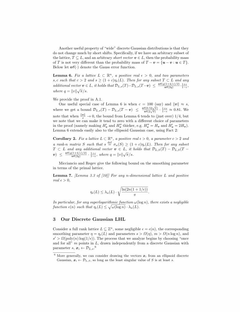
Another useful property of “wide” discrete Gaussian distributions is that theydo not change much by short shifts. Specifically, if we have an arbitrary subset ofthe lattice, T ⊆ L, and an arbitrary short vector v ∈ L, then the probability massof T is not very different than the probability mass of T − v = u− v : u ∈ T.Below let erf(·) denote the Gauss error function.

Lemma 6. Fix a lattice L ⊂ Rn, a positive real ε > 0, and two parameterss, c such that c > 2 and s ≥ (1 + c)ηε(L). Then for any subset T ⊂ L and any

additional vector v ∈ L, it holds that DL,s(T )−DL,s(T−v) ≤ erf(q(1+4/c)/2)erf(2q) · 1+ε1−ε ,

where q = ‖v‖√π/s.

We provide the proof in A.1.One useful special case of Lemma 6 is when c = 100 (say) and ‖v‖ ≈ s,

where we get a bound DL,s(T ) − DL,s(T − v) ≤ erf(0.52√π)

erf(2√π)· 1+ε1−ε ≈ 0.81. We

note that when ‖v‖s → 0, the bound from Lemma 6 tends to (just over) 1/4, butwe note that we can make it tend to zero with a different choice of parametersin the proof (namely making H ′v and H ′′v thicker, e.g. H ′′v = Hv and H ′v = 2Hv).Lemma 6 extends easily also to the ellipsoid Gaussian case, using Fact 2:

Corollary 2. Fix a lattice L ⊂ Rn, a positive real ε > 0, a parameter c > 2 and

a rank-n matrix S such that sdef= σn(S) ≥ (1 + c)ηε(L). Then for any subset

T ⊂ L and any additional vector v ∈ L, it holds that DL,S(T ) − DL,S(T −v) ≤ erf(q(1+4/c)/2)

erf(2q) · 1+ε1−ε , where q = ‖v‖√π/s.

Micciancio and Regev give the following bound on the smoothing parameterin terms of the primal lattice.

Lemma 7. [Lemma 3.3 of [10]] For any n-dimensional lattice L and positivereal ε > 0,

ηε(L) ≤ λn(L) ·√

ln(2n(1 + 1/ε))

π.

In particular, for any superlogarithmic function ω(log n), there exists a negligiblefunction ε(n) such that ηε(L) ≤

√ω(log n) · λn(L).

3 Our Discrete Gaussian LHL

Consider a full rank lattice L ⊆ Zn, some negligible ε = ε(n), the correspondingsmoothing parameter η = ηε(L) and parameters s > Ω(η), m > Ω(n log n), ands′ > Ω(poly(n) log(1/ε)). The process that we analyze begins by choosing “onceand for all” m points in L, drawn independently from a discrete Gaussian withparameter s, xi ← DL,s.6

6 More generally, we can consider drawing the vectors xi from an ellipsoid discreteGaussian, xi ← DL,S , so long as the least singular value of S is at least s.

Once the xi’s are fixed, we arrange them as the columns of an n-by-m matrixX = (x1|x2| . . . |xm), and consider the distribution EX,s′ , induced by choosingan integer vector v from a discrete spherical Gaussian with parameter s′ andoutputting y = X · v:

EX,s′def= X · v : v ← DZm,s′. (1)

Our goal is to prove that EX,s′ is close to the ellipsoid Gaussian DL,s′X> ,over L. We begin by proving that the singular values of X> are all roughly ofthe size s

√m7.

Lemma 8. There exists a universal constant K > 1 such that for all m ≥ 2n,ε > 0 and every n-dimensional real lattice L ⊂ Rn, the following holds: choosingthe rows of an m-by-n matrix X> independently at random from a sphericaldiscrete Gaussian on L with parameter s > 2Kηε(L), X> ← (DL,s)m, we have

Pr[s√

2πm/K < σn(X>) ≤ σ1(X>) < sK√

2πm]> 1−(4mε+O(exp(−m/K))).

The proof can be found in the long version [1].

3.1 The Distribution EX,s′ Over Zn

We next move to show that with high probability over the choice of X, thedistribution EX,s′ is statistically close to the ellipsoid discrete Gaussian DL,s′X> .We first prove this for the special case of the integer lattice, L = Zn, and thenuse that special case to prove the same statement for general lattices. In eithercase, we analyze the setting where the columns of X are chosen from an ellipsoidGaussian which is “not too small” and “not too skewed.”

Parameters. Below n is the security parameters and ε = negligible(n). Let Sbe an n-by-n matrix such that σn(S) ≥ 2Kηε(Zn), and denote s1 = σ1(S),sn = σn(S), and w = s1/sn. (We consider w to be a measure for the “skewness”of S.) Also let m, q, s′ be parameters satisfying m ≥ 10n log q, q > 8m5/2n1/2s1w,and s′ ≥ 4wm3/2n1/2 ln(1/ε). An example setting of parameters to keep in mindis m = n2, sn =

√n (which implies ε ≈ 2−

√n), s1 = n (so w =

√n), q = 8n7,

and s′ = n5.

Theorem 2. For ε negligible in n, let S ∈ Rn×n be a matrix such that sn =σn(S) ≥ 18Kηε(Zn), and denote s1 = σ1(S) and w = s1/sn. Also let m, s′ beparameters such that m ≥ 10n log(8m5/2n1/2s1w) and s′ ≥ 4wm3/2n1/2 ln(1/ε).

Then, when choosing the columns of an n-by-m matrix X from the ellipsoidGaussian over Zn, X ← (DZn,S)m, we have with all but probability 2−O(m)

over the choice of X, that the statistical distance between EX,s′ and the ellipsoidGaussian DZn,s′X> is bounded by 2ε.

7 Since we eventually apply the following lemmas to X>, we will use X> in thestatement of the lemmas for consistency at the risk of notational clumsiness.

The rest of this subsection is devoted to proving Theorem 2. We begin by showingthat with overwhelming probability, the columns of X span all of Zn, whichmeans also that the support of EX,s′ includes all of Zn.

Lemma 9. With parameters as above, when drawing the columns of an n-by-mmatrix X independently at random from DZn,S we get X · Zm = Zn with all butprobability 2−O(m).

The proof can be found in the long version [1].From now on we assume that the columns of X indeed span all of Zn. Now

let A = A(X) be the (m − n)-dimensional lattice in Zm orthogonal to all therows of X, and for any z ∈ Zn we denote by Az = Az(X) the z coset of A:

A = A(X)def= v ∈ Zm : X ·v = 0 and Az = Az(X)

def= v ∈ Zm : X ·v = z.

Since the columns of X span all of Zn then Az is nonempty for every z ∈ Zn,and we have Az = vz +A for any arbitrary point vz ∈ Az.

Below we prove that the smoothing parameter of A is small (whp), and usethat to bound the distance between EX,s′ and DZn,s′X> . First we show that ifthe smoothing parameter of A is indeed small (i.e., smaller than the parameters′ used to sample the coefficient vector v), then EX,s′ and DZn,s′X> must beclose.

Lemma 10. Fix X and A = A(X) as above. If s′ ≥ ηε(A), then for any pointz ∈ Zn, the probability mass assigned to z by EX,s′ differs from that assigned byDZn,s′X> by at most a factor of (1− ε)/(1 + ε), namely

EX,s′(z) ∈[1−ε1+ε , 1

]· DZn,s′X>(z).

In particular, if ε < 1/3 then the statistical distance between EX,s′ and DZn,s′X

is at most 2ε.

The proof can be found in Appendix A.2.

The smoothing parameter of A. We now turn our attention to proving thatA is “smooth enough”. Specifically, for the parameters above we prove that withhigh probability over the choice of X, the smoothing parameter ηε(A) is boundedbelow s′ = 4wm3/2n1/2 ln(1/ε).

Recall again that A = A(X) is the rank-(m − n) lattice containing all theinteger vectors in Zm orthogonal to the rows of X. We extend A to a full-rank lattice as follows: First we extend the rows space of X, by throwing inalso the scaled standard unit vectors qei for the integer parameter q mentionedabove (q ≥ 8m5/2n1/2s1w). That is, we let Mq = Mq(X) be the full-rank m-dimensional lattice spanned by the rows of X and the vectors qei,

Mq = X>z+qy : z ∈ Zn,y ∈ Zm = u ∈ Zm : ∃z ∈ Znq s.t. u ≡ X>z (mod q)

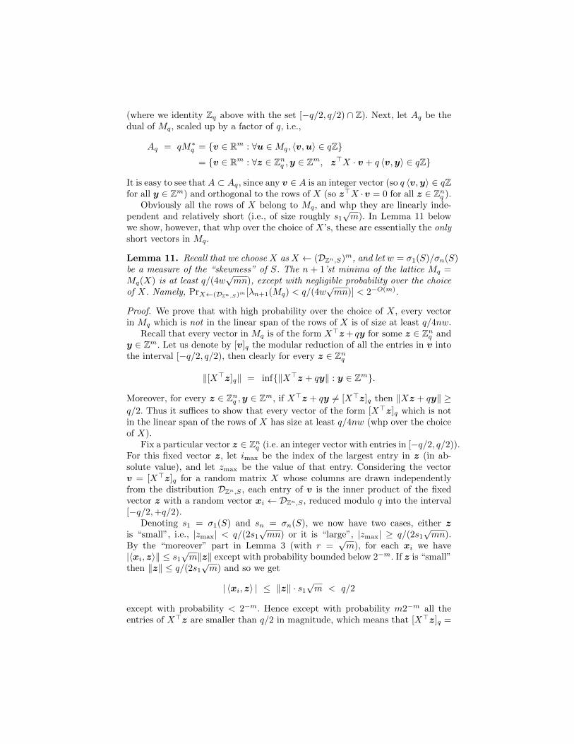
(where we identity Zq above with the set [−q/2, q/2) ∩ Z). Next, let Aq be thedual of Mq, scaled up by a factor of q, i.e.,

Aq = qM∗q = v ∈ Rm : ∀u ∈Mq, 〈v,u〉 ∈ qZ= v ∈ Rm : ∀z ∈ Znq ,y ∈ Zm, z>X · v + q 〈v,y〉 ∈ qZ

It is easy to see that A ⊂ Aq, since any v ∈ A is an integer vector (so q 〈v,y〉 ∈ qZfor all y ∈ Zm) and orthogonal to the rows of X (so z>X ·v = 0 for all z ∈ Znq ).

Obviously all the rows of X belong to Mq, and whp they are linearly inde-pendent and relatively short (i.e., of size roughly s1

√m). In Lemma 11 below

we show, however, that whp over the choice of X’s, these are essentially the onlyshort vectors in Mq.

Lemma 11. Recall that we choose X as X ← (DZn,S)m, and let w = σ1(S)/σn(S)be a measure of the “skewness” of S. The n + 1’st minima of the lattice Mq =Mq(X) is at least q/(4w

√mn), except with negligible probability over the choice

of X. Namely, PrX←(DZn,S)m [λn+1(Mq) < q/(4w√mn)] < 2−O(m).

Proof. We prove that with high probability over the choice of X, every vectorin Mq which is not in the linear span of the rows of X is of size at least q/4nw.

Recall that every vector in Mq is of the form X>z+ qy for some z ∈ Znq andy ∈ Zm. Let us denote by [v]q the modular reduction of all the entries in v intothe interval [−q/2, q/2), then clearly for every z ∈ Znq

‖[X>z]q‖ = inf‖X>z + qy‖ : y ∈ Zm.

Moreover, for every z ∈ Znq ,y ∈ Zm, if X>z + qy 6= [X>z]q then ‖Xz + qy‖ ≥q/2. Thus it suffices to show that every vector of the form [X>z]q which is notin the linear span of the rows of X has size at least q/4nw (whp over the choiceof X).

Fix a particular vector z ∈ Znq (i.e. an integer vector with entries in [−q/2, q/2)).For this fixed vector z, let imax be the index of the largest entry in z (in ab-solute value), and let zmax be the value of that entry. Considering the vectorv = [X>z]q for a random matrix X whose columns are drawn independentlyfrom the distribution DZn,S , each entry of v is the inner product of the fixedvector z with a random vector xi ← DZn,S , reduced modulo q into the interval[−q/2,+q/2).

Denoting s1 = σ1(S) and sn = σn(S), we now have two cases, either zis “small”, i.e., |zmax| < q/(2s1

√mn) or it is “large”, |zmax| ≥ q/(2s1

√mn).

By the “moreover” part in Lemma 3 (with r =√m), for each xi we have

|〈xi, z〉‖ ≤ s1√m‖z‖ except with probability bounded below 2−m. If z is “small”

then ‖z‖ ≤ q/(2s1√m) and so we get

| 〈xi, z〉 | ≤ ‖z‖ · s1√m < q/2

except with probability < 2−m. Hence except with probability m2−m all theentries of X>z are smaller than q/2 in magnitude, which means that [X>z]q =

X>z, and so [X>z]q belongs to the row space of X. Using the union boundagain, we get that with all but probability qn ·m2−m < m2−9m/10, the vectors[X>z]q for all the “small” z’s belong to the row space of X.

We next turn to analyzing “large” z’s. Fix one “large” vector z, and forthat vector define the set of “bad” vectors x ∈ Zn, i.e. the ones for which|[〈z,x〉]q| < q/4nw (and the other vectors x ∈ Zn are “good”). Observe that ifx is “bad”, then we can get a “good” vector by adding to it the imax’th standardunit vector, scaled up by a factor of µ = min

(dsne , bq/|2zmax|c

), since

|[〈z,x+ µeimax〉]q| = |[〈z,x〉+ µzmax]q| ≥ µ|zmax| − |[〈z,x〉]q| ≥ q/4nw.

(The last two inequalities follow from q/2nw < µ|zmax| ≤ q/2 and |[〈z,x〉]q| <q/(4w

√mn).) Hence the injunction x 7→ x+ µeimax

maps “bad” x’es to “good”x’es. Moreover, since the x’es are chosen according to the wide ellipsoid Gaus-sian DZn,S with σn(S) = sn ≥ ηε(Zn), and since the scaled standard unitvectors are short, µ < sn + 1, then by Lemma 6 the total probability massof the “bad” vectors x differs from the total mass of the “good” vectors x +µeimax by at most 0.81. It follows that when choosing x ← DZn,S , we havePrx [|[〈z,x〉]q| < q/(4w

√mn)] ≤ (1 + 0.81)/2 < 0.91. Thus the probability that

all the entries of [X>z]q are smaller than q/(4w√nm) in magnitude is bounded

by (0.91)m = 2−0.14m. Since m > 10n log q, we can use the union bound toconclude that the probability that there exists some “large” vector for which‖[X>z]q‖ < q/(4w

√mn) is no more than qn · 2−0.14m < 2−O(m).

Summing up the two cases, with all but probability 2−O(m)) over the choiceof X, there does not exist any vector z ∈ Znq for which [X>z]q is linearly

independent of the rows of X and yet |[X>z]q| < q/(4w√mn).

Corollary 3. With the parameters as above, the smoothing parameter of A =A(X) satisfies ηε(A) ≤ s′ = 4wm3/2n1/2 ln(1/ε), except with probability 2−O(m).

The proof can be found in the long version [1].Putting together Lemma 10 and Corollary 3 completes the proof of Theorem 2.

ut

3.2 The Distribution EX,s′ Over General Lattices

Armed with Theorem 2, we turn to prove the same theorem also for generallattices.

Theorem 3. Let L be a full-rank lattice L ⊂ Rn and B a matrix whose columnsform a basis of L. Also let M ∈ Rn×n be a full rank matrix, and denote S =M(B>)−1, s1 = σ1(S), sn = σn(S), and w = s1/sn. Finally let ε be negligiblein n and m, s′ be parameters such that m ≥ 10n log(8m5/2n1/2s1w) and s′ ≥4wm3/2n1/2 ln(1/ε).

If sn ≥ ηε(Zn), then, when choosing the columns of an n-by-m matrix X fromthe ellipsoid Gaussian over L, X ← (DL,M )m, we have with all but probability2−O(m) over the choice of X, that the statistical distance between EX,s′ and theellipsoid Gaussian DL,s′X> is bounded by 2ε.

This theorem is an immediate corollary of Theorem 2 and Fact 2. The proofcan be found in the long version [1].

4 Applications

In this section, we discuss the application of our discrete Gaussian LHL in theconstruction of multilinear maps from lattices [5]. This construction is illustrativeof a “canonical setting” where our lemma should be useful.

Brief overview of the GGH Construction. To begin, we provide a very high leveloverview of the GGH construction, skipping most details. We refer the reader to[5] for a complete description. In [5], the mapping a→ ga from bilinear maps isviewed as a form of “encoding” a 7→ Enc(a) that satisfies some properties:

1. Encoding is easy to compute in the forward direction and hard to invert.2. Encoding is additively homomorphic and also one-time multiplicatively ho-

momorphic (via the pairing).3. Given Enc(a), Enc(b) it is easy to test whether a = b.4. Given encodings, it is hard to test more complicated relations between the

underlying scalars. For example, BDDH roughly means that given Enc(a),Enc(b), Enc(c), Enc(d) it is hard to test if d = abc.

In [5], the authors construct encodings from ideal lattices that approximatelysatisfy (and generalize) the above properties. Skipping most of the details, [5]roughly used a specific (NTRU-like) lattice-based homomorphic encryption scheme,where Enc(a) is just an encryption of a. The ability to add and multiply thenjust follows from the homomorphism of the underlying cryptosystem, and GGHdescribed how to add to this cryptosystem a “broken secret key” that cannotbe used for decryption but is good enough for testing if two ciphertexts encryptthe same element. (In the terminology from [5], this broken key is called thezero-test parameter.)

In the specific cryptosystem used in the GGH construction, ciphertexts areelements in some polynomial ring (represented as vectors in Zn), and addi-tive/multiplicative homomorphism is implemented simply by addition and mul-tiplication in the ring. A natural way to enable encoding is to publish a sin-gle ciphertext that encrypts/encodes 1, y1 = Enc(1). To encode any otherplaintext element a, we can use the multiplicative homomorphism by settingEnc(a) = a · y1 in the ring. However this simple encoding is certainly not hardto decode: just dividing by y1 in the ring suffices! For the same reason, it is alsonot hard to determine “complex relations” between encoding.

Randomizing the encodings. To break these simple algebraic relations, the au-thors include in the public parameters also “randomizers” xi (i = 1, . . . ,m),which are just random encryptions/encodings of zero, namely xi ← Enc(0).Then to re-randomize the encoding ua = a · y1, they add to it a “random lin-ear combination” of the xi’s, and (by additive homomorphism) this is another

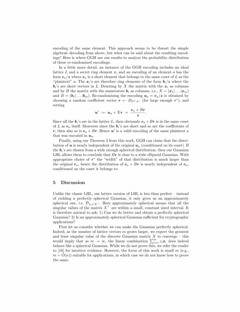
encoding of the same element. This approach seems to be thwart the simplealgebraic decoding from above, but what can be said about the resulting encod-ings? Here is where GGH use our results to analyze the probability distributionof these re-randomized encodings.

In a little more detail, an instance of the GGH encoding includes an ideallattice L and a secret ring element z, and an encoding of an element a has theform ea/z where ea is a short element that belongs to the same coset of L as the“plaintext” a. The xi’s are therefore ring elements of the form bi/z where thebi’s are short vectors in L. Denoting by X the matrix with the xi as columnsand by B the matrix with the numerators bi as columns, i.e., X = (x1| . . . |xm)and B = (b1| . . . |bm). Re-randomizing the encoding ua = ea/z is obtained bychoosing a random coefficient vector r ← DZm,σ∗ (for large enough σ∗), andsetting

u′ := ua +Xr =ea +Br

z.

Since all the bi’s are in the lattice L, then obviously ea+Br is in the same cosetof L as ea itself. Moreover since the bi’s are short and so are the coefficients ofr, then also so is ea +Br. Hence u′ is a valid encoding of the same plaintext athat was encoded in ua.

Finally, using our Theorem 3 from this work, GGH can claim that the distri-bution of u is nearly independent of the original ua (conditioned on its coset). Ifthe bi’s are chosen from a wide enough spherical distribution, then our GaussianLHL allows them to conclude that Br is close to a wide ellipsoid Gaussian. Withappropriate choice of σ∗ the “width” of that distribution is much larger thanthe original ea, hence the distribution of ea + Br is nearly independent of ea,conditioned on the coset it belongs to.

5 Discussion

Unlike the classic LHL, our lattice version of LHL is less than perfect – insteadof yielding a perfectly spherical Gaussian, it only gives us an approximatelyspherical one, i.e. DL,s′X> . Here approximately spherical means that all thesingular values of the matrix X> are within a small, constant sized interval. Itis therefore natural to ask: 1) Can we do better and obtain a perfectly sphericalGaussian? 2) Is an approximately spherical Gaussian sufficient for cryptographicapplications?

First let us consider whether we can make the Gaussian perfectly spherical.Indeed, as the number of lattice vectors m grows larger, we expect the greatestand least singular value of the discrete Gaussian matrix X to converge – thiswould imply that as m → ∞, the linear combination

∑mi=1 zixi does indeed

behave like a spherical Gaussian. While we do not prove this, we refer the readerto [16] for intuitive evidence. However, the focus of this work is small m (e.g.,m = O(n)) suitable for applications, in which case we do not know how to provethe same.

This leads to the second question: is approximately spherical good enough?This depends on the application. We have already seen that it is sufficient forGGH encodings [5], where a canonical, wide-enough, but non-spherical Gaussianis used to “drown out” an initial encoding, and send it to a canonical distribu-tion of encodings that encode the same value. Our LHL shows that one cansample from such a canonical approximate Gaussian distribution without usingthe initial Gaussian samples “wastefully”.

On the other hand, we caution the reader that if the application requires thebasis vectors x1, . . . ,xm to be kept secret (such as when the basis is a trapdoor),then one must carefully consider whether our Gaussian sampler can be usedsafely. This is because, as demonstrated by [11] and [4], lattice applicationswhere the basis is desired to be secret can be broken completely even if partialinformation about the basis is leaked. In an application where the trapdoor isavailable explicitly and oblivious sampling is not needed, it is safer to use thesamplers of [6] or [13] to sample a perfectly spherical Gaussian that is statisticallyindependent of the trapdoor.

Acknowledgments. The first and fourth authors were supported in part from aDARPA/ONR PROCEED award, NSF grants 1228984, 1136174, 1118096, and1065276, a Xerox Faculty Research Award, a Google Faculty Research Award, anequipment grant from Intel, and an Okawa Foundation Research Grant. This ma-terial is based upon work supported by the Defense Advanced Research ProjectsAgency through the U.S. Office of Naval Research under Contract N00014-11-1-0389. The views expressed are those of the author and do not reflect the officialpolicy or position of the Department of Defense, the National Science Founda-tion, or the U.S. Government.

The second and third authors were supported by the Intelligence AdvancedResearch Projects Activity (IARPA) via Department of Interior National Busi-ness Center (DoI/NBC) contract number D11PC20202. The U.S. Governmentis authorized to reproduce and distribute reprints for Governmental purposesnotwithstanding any copyright annotation thereon. Disclaimer: The views andconclusions contained herein are those of the authors and should not be inter-preted as necessarily representing the official policies or endorsements, eitherexpressed or implied, of IARPA, DoI/NBC, or the U.S. Government.

References

1. Shweta Agrawal, Craig Gentry, Shai Halevi, and Amit Sahai. Discrete gaussianleftover hash lemma over infinite domains. http://eprint.iacr.org/2012/714,2012.

2. Wojciech Banaszczyk. New bounds in some transference theorems in the geometryof numbers. Mathematische Annalen, 296(4):625–635, 1993.

3. Dan Boneh and David Mandall Freeman. Homomorphic signatures for polynomialfunctions. In Eurocrypt, volume 6632 of Lecture Notes in Computer Science, pages149–168. Springer, 2011.

4. Leo Ducas and Phong Q. Nguyen. Learning a zonotope and more: Cryptanalysisof ntrusign countermeasures. In ASIACRYPT, volume 7658 of Lecture Notes inComputer Science, pages 433–450, 2012.

5. Sanjam Garg, Craig Gentry, and Shai Halevi. Candidate multilinear maps fromideal lattices and applications. In Eurocrypt, volume 7881 of Lecture Notes inComputer Science, pages 1–17. Springer, 2013. Full version in http://eprint.

iacr.org/2013/610.

6. Craig Gentry, Chris Peikert, and Vinod Vaikuntanathan. Trapdoors for hard lat-tices and new cryptographic constructions. In Cynthia Dwork, editor, STOC, pages197–206. ACM, 2008.

7. Philip Klein. Finding the closest lattice vector when it’s unusually close. In Pro-ceedings of the eleventh annual ACM-SIAM symposium on Discrete algorithms,SODA’00, pages 937–941, 2000.

8. A. E. Litvak, A. Pajor, M. Rudelson, and N. Tomczak-Jaegermann. Smallestsingular value of random matrices and geometry of random polytopes. Advancesin Mathematics, 195(2), 2005.

9. Vadim Lyubashevsky. Lattice signatures without trapdoors. In Eurocrypt, volume7237 of Lecture Notes in Computer Science, pages 738–755. Springer, 2012.

10. Daniele Micciancio and Oded Regev. Worst-case to average-case reductions basedon gaussian measures. SIAM J. Computing, 37(1):267–302, 2007.

11. Phong Q. Nguyen and Oded Regev. Learning a parallelepiped: Cryptanalysis ofGGH and NTRU signatures. J. Cryptol., 22(2):139–160, April 2009.

12. Chris Peikert. Limits on the hardness of lattice problems in lp norms. Computa-tional Complexity, 17(2):300–351, 2008.

13. Chris Peikert. An efficient and parallel gaussian sampler for lattices. In Crypto,volume 6223 of Lecture Notes in Computer Science, pages 80–97. Springer, 2010.

14. Oded Regev. On lattices, learning with errors, random linear codes, and cryptog-raphy. JACM, 56(6), 2009.

15. Ron Rothblum. Homomorphic encryption: From private-key to public-key. In TCC,volume 6597 of Lecture Notes in Computer Science, pages 219–234. Springer, 2011.

16. Mark Rudelson and Roman Vershynin. Non-asymptotic theory of random matrices:extreme singular values. In International Congress of Mathematicans, 2010.

17. Terence Tao. Topics in random matrix theory, volume 132 of Graduate Studies inMathematics. American Mathematical Society, 2012.

18. Marten van Dijk, Craig Gentry, Shai Halevi, and Vinod Vaikuntanathan. Fullyhomomorphic encryption over the integers. In Henri Gilbert, editor, Advances inCryptology - EUROCRYPT’10, volume 6110 of Lecture Notes in Computer Science,pages 24–43. Springer, 2010.

A More Proofs

A.1 Proof of Lemma 6

Proof. Clearly for any fixed v, the set that maximizes DL,s(T ) − DL,s(T − v)is the set of all vectors u ∈ L for which DL,s(u) > DL,s(u − v), which we

denote by Tvdef= u ∈ L : DL,s(u) > DL,s(u− v). Observe that for any u ∈ L

we have DL,s(u) > DL,s(u − v) iff ρs(u) > ρs(u − v), which is equivalent to

‖u‖ < ‖u − v‖. That is, u must lie in the half-space whose projection on v isless than half of v, namely 〈u,v〉 < ‖v‖2/2. In other words we have

Tv = u ∈ L : 〈u,v〉 < ‖v‖2/2,

which also means that Tv − v = u ∈ L : 〈u,v〉 < −‖v‖2/2 ⊆ Tv. We cantherefore express the difference in probability mass as DL,s(Tv)−DL,s(Tv−v) =DL,s(Tv \ (Tv − v)). Below we denote this set-difference by

Hvdef= Tv \ (Tv − v) =

u ∈ L : 〈u,v〉 ∈ (−‖v‖

2

2 , ‖v‖2

2 ].

That is, Hv is the “slice” in space of width ‖v‖ in the direction of v, which issymmetric around the origin. The arguments above imply that for any set T wehaveDL,s(T )−DL,s(T−v) ≤ DL,s(Hv). The rest of the proof is devoted to upper-bounding the probability mass of that slice, i.e., DL,s(Hv) = Pru←DL,s

[u ∈ Hv].To this end we consider the slightly thicker slice, say H ′v = (1+ 4

c )Hv, and therandom variable w, which is obtained by drawing u← DL,s and adding to it acontinuous Gaussian variable of “width” s/c. We argue thatw is somewhat likelyto fall outside of the thick slice H ′v, but conditioning on u ∈ Hv we have thatw is very unlikely to fall outside of H ′v. Putting these two arguments together,we get that u must have significant probability of falling outside Hv, therebygetting our upper bound.

In more detail, denoting r = s/c we consider drawing u ← DL,s and z ←Nn(0, r2/2π), and setting w = u + z. Denoting t =

√r2 + s2, we have that

s ≤ t ≤ s(1 + 1c ) and rs/t ≥ s/(c+ 1) ≥ ηε(L). Thus the conditions of Lemma 5

are met, and we get that w is distributed close to a normal random variableNn(0, t2/2π), upto a factor of at most 1+ε

1−ε .Since the continuous Gaussian distribution is spherical, we can consider ex-

pressing it in an orthonormal basis with one vector in the direction of v. Whenexpressed in this basis, we get the event z ∈ H ′v exactly when the coefficientin the direction of v (which is distributed close to the 1-dimensional GaussianN (0, t2/2π)) exceeds ‖v(1 + 4

c )/2‖ in magnitude. Hence we have

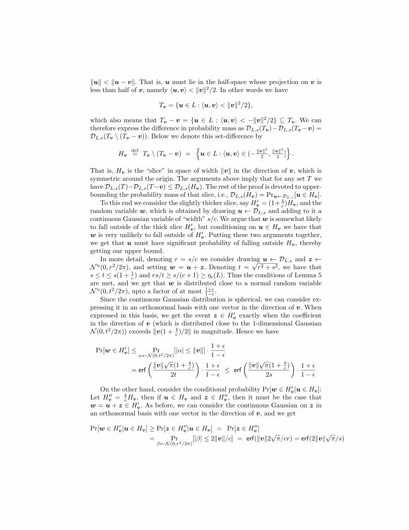
Pr[w ∈ H ′v] ≤ Prα←N (0,t2/2π)

[|α| ≤ ‖v‖] · 1 + ε

1− ε

= erf

(‖v‖√π(1 + 4c )

2t

)· 1 + ε

1− ε≤ erf

(‖v‖√π(1 + 4c )

2s

)· 1 + ε

1− ε

On the other hand, consider the conditional probability Pr[w ∈ H ′v|u ∈ Hv]:Let H ′′v = 4

cHv, then if u ∈ Hv and z ∈ H ′′v , then it must be the case thatw = u + z ∈ H ′v. As before, we can consider the continuous Gaussian on z inan orthonormal basis with one vector in the direction of v, and we get

Pr[w ∈ H ′v|u ∈ Hv] ≥ Pr[z ∈ H ′′v |u ∈ Hv] = Pr[z ∈ H ′′v ]

= Prβ←N (0,r2/2π)

[|β| ≤ 2‖v‖/c] = erf(‖v‖2√π/cr) = erf(2‖v‖

√π/s)

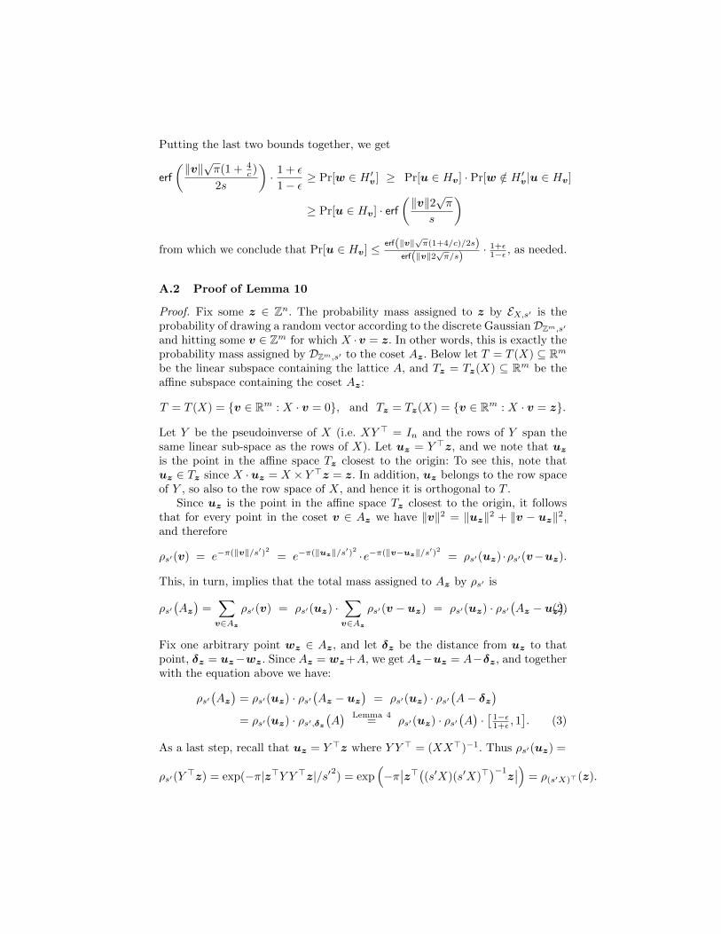
Putting the last two bounds together, we get

erf

(‖v‖√π(1 + 4c )

2s

)· 1 + ε

1− ε≥ Pr[w ∈ H ′v] ≥ Pr[u ∈ Hv] · Pr[w /∈ H ′v|u ∈ Hv]

≥ Pr[u ∈ Hv] · erf(‖v‖2

√π

s

)

from which we conclude that Pr[u ∈ Hv] ≤ erf(‖v‖√π(1+4/c)/2s)

erf(‖v‖2√π/s)

· 1+ε1−ε , as needed.

A.2 Proof of Lemma 10

Proof. Fix some z ∈ Zn. The probability mass assigned to z by EX,s′ is theprobability of drawing a random vector according to the discrete Gaussian DZm,s′

and hitting some v ∈ Zm for which X ·v = z. In other words, this is exactly theprobability mass assigned by DZm,s′ to the coset Az. Below let T = T (X) ⊆ Rmbe the linear subspace containing the lattice A, and Tz = Tz(X) ⊆ Rm be theaffine subspace containing the coset Az:

T = T (X) = v ∈ Rm : X · v = 0, and Tz = Tz(X) = v ∈ Rm : X · v = z.

Let Y be the pseudoinverse of X (i.e. XY > = In and the rows of Y span thesame linear sub-space as the rows of X). Let uz = Y >z, and we note that uzis the point in the affine space Tz closest to the origin: To see this, note thatuz ∈ Tz since X ·uz = X × Y >z = z. In addition, uz belongs to the row spaceof Y , so also to the row space of X, and hence it is orthogonal to T .

Since uz is the point in the affine space Tz closest to the origin, it followsthat for every point in the coset v ∈ Az we have ‖v‖2 = ‖uz‖2 + ‖v − uz‖2,and therefore

ρs′(v) = e−π(‖v‖/s′)2 = e−π(‖uz‖/s′)2 ·e−π(‖v−uz‖/s′)2 = ρs′(uz) ·ρs′(v−uz).

This, in turn, implies that the total mass assigned to Az by ρs′ is

ρs′(Az)

=∑v∈Az

ρs′(v) = ρs′(uz) ·∑v∈Az

ρs′(v − uz) = ρs′(uz) · ρs′(Az − uz

).(2)

Fix one arbitrary point wz ∈ Az, and let δz be the distance from uz to thatpoint, δz = uz−wz. Since Az = wz+A, we get Az−uz = A−δz, and togetherwith the equation above we have:

ρs′(Az)

= ρs′(uz) · ρs′(Az − uz

)= ρs′(uz) · ρs′

(A− δz

)= ρs′(uz) · ρs′,δz

(A) Lemma 4

= ρs′(uz) · ρs′(A)·[1−ε1+ε , 1

]. (3)

As a last step, recall that uz = Y >z where Y Y > = (XX>)−1. Thus ρs′(uz) =

ρs′(Y>z) = exp(−π|z>Y Y >z|/s′2) = exp

(−π∣∣z>((s′X)(s′X)>

)−1z∣∣) = ρ(s′X)>(z).

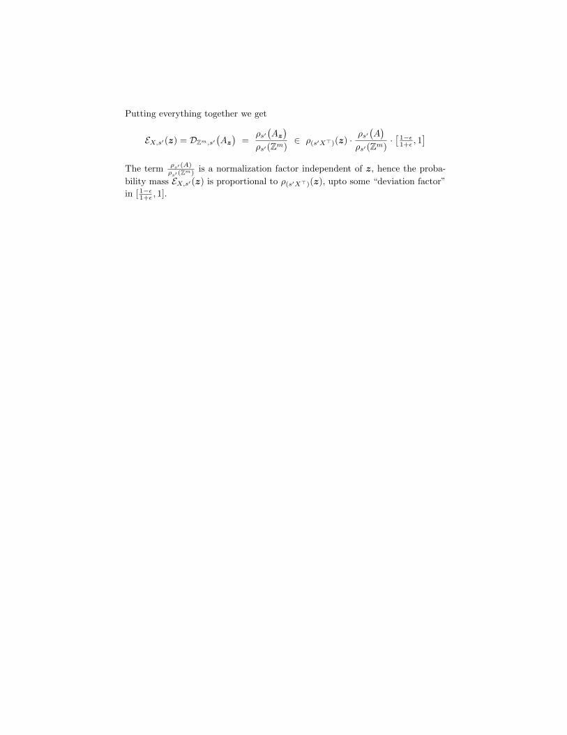
Putting everything together we get

EX,s′(z) = DZm,s′(Az)

=ρs′(Az)

ρs′(Zm)∈ ρ(s′X>)(z) ·

ρs′(A)

ρs′(Zm)·[1−ε1+ε , 1

]The term ρs′ (A)

ρs′ (Zm) is a normalization factor independent of z, hence the proba-

bility mass EX,s′(z) is proportional to ρ(s′X>)(z), upto some “deviation factor”

in [ 1−ε1+ε , 1].