Discrete Event Simulation and Production System Design for ...

Discrete Event Simulation and Production System Designfor Rockwell Hardness Test Blocks

ByDavid Eliot Scheinman

B.S. Mechanical EngineeringUniversity of California at Davis, 2005

SUBMITTED TO THE DEPARTMENT OF MECHANICAL ENGINEERING INPARTIAL FULFILLMENT OF THE REQUIREMENTS FOR THE DEGREE OF

Master of Engineering in Manufacturing

AT THEMASSACHUSETTS INSTITUTE OF TECHNOLOGY

August 2009

© 2009 David Eliot Scheinman. All rights reserved

The author hereby grants to MIT permission to reproduce and to distribute publicly paper andelectronic copies of this thesis document in whole or in part in any medium now known or

hereafter created.

Signature of Author:

Certified by:K-'

6)Accepted by:_

Department of Mechanical EngineeringAugust 18 2009

_ _ Jung-Hoon ChunProfessor of Mechanical Engineering

Thesis Supervisor

David E. HardtChairman, Committee for Graduate Students

ARCHIVES

MASSACHUSETTS INsTfUT-EOF TECHNOLOGY

DEC 2 8 2009

LIBRARIES

Discrete Event Simulation and Production System Design for

Rockwell Hardness Test Blocks

By

David Eliot Scheinman

Submitted to the Department of Mechanical Engineering on

August 18, 2009 in partial fulfillment of the requirements for the

Degree of Master of Engineering in Manufacturing.

Abstract

The research focuses on increasing production volume and decreasing costs at a hardness test

block manufacturer. A discrete event simulation model is created to investigate potential system

wide improvements. Using the results from the simulation a production work-cell is proposed

that will allow a single worker to operate 7 machines at a rate that exceeds existing production

rates. This results in the workforce being reduced by a factor of four while reducing product

lead-time by 30% and increasing throughput by 50%.

Thesis Supervisor: Dr. Jung-Hoon Chun

Title: Professor of Mechanical Engineering

Table of Contents

Abstract .......................... ................................................................................................................................. 2

Table of Contents .................................................... 3

List of Figures and Tables.................................................................................. .................................... 4

Chapter 1: Introduction ..................................................... 51.1 Corporate Background .................................................... 51.2 Rockwell H ardness Testing Background ................................................................................................................... 51.3 M anufacturing process ..................................................................................................................................................... 61.4 Problem Statem ent ............................................................................................................................................................ 9

Chapter 2: Literature R eview .................................................... 113.1 M odel D esign...................................................................................................................................................................... 123.2 Data Acquisition ................................................................................................................................................................ 143.2 Data Acquisition........................................3.3 M odel Validation ............................................................................................................................................................... 16

Chapter 4: R esults .............................................................................................................................................. 194.1 Existing System ................................................................................................................................................................... 194.2 Polishing Improvements ................................................................................................................................... 214.3 M axim izing Efficiency at Expected D emand Levels ...................................................................................... 24

Chapter 5: Conclusions and Recom m endations .......................................................................................... 29

Appendix A : Sim ulation Code ................................................... 31Usage: ........................................................................................................................................................................................... 31Usage Notes:............................................................................................................................................................................... 31Code: ............................................................................................................................................................................................. 31

Appendix B: Exam ple Data File ...................................................................................................................... 37

Appendix C : V ariables ...................................................................................................................................... 39

Appendix D: ASTM E18-08a ........................................ ................................................................ 40

References ........................................................................................................................................................... 41

List of Figures and Tables

Figure 1: Test Block Manufacturing Process Flow Chart ............................................... 8

Figure 2: Node structure utilized to simulate the production process ..................................... 13

Figure 3: Sample lead time by part type of the existing system. Parts Types 0-7 represent brassparts while 8-15 represent steel parts. ...................................................................... 17

Figure 4: Queue length of the steel polishing machine ................................................................ 18

Figure 5: Production rate over time of the existing production system. Demand rate is 30,000parts per year. ........................................................................................................................ 20

Figure 6: Queue length for the steel polishing node at a demand rate of 30,000 parts per year..20

Figure 7: Queue length for the brass polishing node at a demand rate of 30,000 parts per year.. 21

Figure 8: Production rate over time with the proposed improvements to the polishing process.D em and rate is 48,000 parts/year. ......................................................................................... 22

Figure 9: Queue length over time for the bras polishing node at a demand rate of 48,000 partsper year. ................................................................ .................................................................... 23

Figure 10: Queue length over time for the grinding node at a demand rate of 48,000 parts pery ear. ....................................................................................................................................... 2 3

Figure 11: Production rate vs. time with proposed polishing improvements and a single workerwith a demand rate of 25,000 parts per year. ................................................ 24

Figure 12: System production rate with a 15% rework rate at the buffing stage ...................... 27

Figure 13: System production rate with a 25% rework rate at the polishing stage ................... 27

Figure 14: Single worker production with proposed improvements to the initial turning

processes............................................... .................................................... ...................... 2 8

Table 1: Aggregated production and rework rates for each process. (s) deontes steel parts, (b)denotes brass parts .................................................................................................................. 16

Table 2: Proposed production schedule for up to 22,500 parts per year with a single worker. ... 25

Chapter 1: Introduction

This thesis is sponsored by Wilson Instruments. It is focused on improving the productivity and

throughput of the production line dedicated to manufacturing metal calibration blocks used to

calibrate Wilson's Rockwell hardness testing equipment. Over the course of a 7-month

internship, we have analyzed and improved the production process of the calibration blocks.

1.1 Corporate Background

Wilson Instruments, a subsidiary of Illinois Tool Works (ITW), has been a pioneer in hardness

testing equipment and standards. The company was founded by Charles H. Wilson. In 1920,

Charles Wilson collaborated with Stanley Rockwell to produce the first commercially available

Rockwell hardness testing machines. The Rockwell Hardness standard has become the

prominent hardness testing standard for metals. Since their original success with Rockwell

hardness testers, Wilson Instruments has continued to be a market leader in hardness testing with

an expanded instrument line including micro hardness and Brinell hardness testing equipment.

1.2 Rockwell Hardness Testing Background

The Rockwell hardness scale is used to define the indentation hardness of metals. There are

multiple Rockwell scales. For this project we are focused on the Rockwell-B (HRB) and

Rockwell-C (HRC) scales.

The Rockwell hardness test uses a calibrated machine to apply a known force to a diamond or

tungsten-carbide indenter in accordance with ASTM E18-08a. In order to calibrate the testing

machine, a material of a known hardness is tested, and the machine is adjusted so that it reads

correctly. The specifications of the blocks are described in ASTM E18-08a. According to the

standard, Rockwell hardness testing machines shall be verified on a daily basis by means of

standardized test blocks. These test blocks are manufactured and calibrated in accordance with

ASTM E18-02 as shown in Appendix D. The Rockwell test blocks provide an easy and

inexpensive way to verify the machine. These blocks are used as a standard reference to verify

the hardness tester. Due to the destructive nature of the Rockwell indentation test, each time a

calibration block is used a small indentation is left on the block. This means that each block can

only be used 100-200 times before it must be replaced. As a result, Wilson Instruments

manufactures the calibration blocks in large quantities and sells them as consumables.

1.3 Manufacturing Process

The Rockwell test blocks are circular discs approximately 2.5" (63.5mm) in diameter and 0.25"

(6.35mm) thick. The Rockwell test blocks are made from two different materials to provide a full

range of hardness. Cartridge brass is used for test blocks ranging from HRB30 to HRB90, while

0-1 tool steel is used for harder materials up to HRC-60. The test blocks are physically identical,

regardless of material, except for the varying hardness. However, the manufacturing processes

are slightly different for each material. Figure 1 shows the manufacturing process of both types

of Rockwell test blocks.

Wilson manufactures the test blocks at Instron's machine shop in Binghamton, New York. The

manufacturing process is as follows:

1. Brass test blocks are rough cut from 0.350" (8.89mm) brass plates by water jet. Steel blocks

are rough cut with a band saw from round bar stock. Both steel and brass cutting processes

are outsourced and then shipped to the Binghamton facility.

2. At the Binghamton facility a CNC lathe is used to cut the final diameter, face the blocks, and

chamfer the edges. This is performed in two setups. The machined blocks are then roll

stamped with a unique serial number on the circumference.

3. The test blocks are then sent out for heat treatment. The blocks are heat treated to full

hardness and then annealed down to the desired hardness level.

4. When the blocks return from the heat treating facility they have a scaled finish. The blocks

are bead blasted to remove this surface. The blocks are then manually buffed to remove any

sharp edges.

5. The steel blocks are surface ground to ensure proper parallelism.

6. All the blocks are lapped and polished to ensure proper parallelism, surface flatness, and

surface finish.

7. After passing dimensional quality control the blocks are sent to Instron's Norwood facility.

8. At the Norwood facility the hardness of every block is tested and recorded. The blocks are

then packaged and shipped out.

N

Y

I Brass Inhouse I Y

Figure 1: Test Block Manufacturing Process Flow Chart

1.4 Problem Statement

Many of the steps involve high rates of rework, parts often fail final QC due to unknown causes,

and training new workers has been difficult as many of the processes are not properly understood

or documented. Instron wants to investigate the entire manufacturing process to find ways to

streamline the process in order to improve productivity by reducing costs, lead time, and

expanding the potential manufacturing capacity to allow for future increased demand.

During our first month of work we visited the calibration and packaging facility in Norwood, the

production facility in Binghamton and key outside vendors. We interviewed and observed as

many people as possible who were involved with producing the test blocks. Throughout this

process we noticed several reoccurring themes and problems.

The most striking problem we noticed is that the later stages of the manufacturing line, polishing

and lapping, have substantially higher rework rates than the other stages. Both operators and

management complained that cycle times are very inconsistent at these stages. Parts are often

scratched during polishing or lapping, which requires them to be sent back several steps in the

sequence as shown in Figure 1. Some operators are able to produce consistent, high quality parts

while other operators struggle to produce any good parts. We concluded that the polishing and

lapping processes were poorly understood and poorly defined. Mohammd Imani Nejad has

dedicated his efforts to improving the polishing and lapping processes. [5]

While the majority of defects become apparent in the final steps of lapping and polishing, there

were many signals indicating the defects were not necessarily caused by the actual lapping and

polishing processes. Latent defects created during turning, heat-treating, and grinding were

going undetected until late in the production process when rework is more difficult and costly.

Jairaj Vora has dedicated his efforts to discovering and quantifying the sources of variation

caused during all steps preceding lapping. [8]

Vincent Tan focused on reducing the rate of rejected parts at the final stage of the test block

manufacturing by identifying the significant factors from the heat treatment process that affect

the mean hardness and uniformity of the test block. He has also dedicated his efforts to

improving the current sampling methods to provide a better understanding of the mean hardness

and hardness ranges at different stages of the production line. [7]

In the larger picture, the entire production process appears to be rather disorganized. Human

resources are sparsely distributed across several machines causing some of the machines to often

sit idle. This thesis will focus on creating a simulation model to explore strategies for organizing

and distributing the limited machine and human resources to meet the demand in the most cost

effective way possible. The model will also be used to explore the system wide impacts of the

findings of Jairaj Vora's, Mohammad Imani Nejad's, and Vincent Tan's thesis.

Chapter 2: Literature Review

The goal is to create an accurate model of the entire production system, starting with the turning

processing and ending with the polishing process. Avrill Law presents critical decisions to make

when selecting a model type [2]. It is proposed that the ideal solution would be to run tests on

the actual system, unfortunately due to cost time restraints this is not feasible. Short of that,

creating a physical model or a closed form analytical model would also be preferred but are also

not feasible due to time, money, and complexity constraints. With the realm of simulation

models we are interested in a model that will account the dynamic and stochastic nature of the

system.

Within the realm of dynamic, stochastic simulations there are two main types: continuous time

and discrete time simulations. The hardness test block production lends itself well to a discrete

event simulation. The information we are interested in from the simulation is discrete by nature:

the completion of a parts at all production stages, the length of the queues for workers and

machines, the time it takes an order to propagate through the system, and the total number of

parts in the system at any given time.

Chapter 3: Simulation Model

3.1 Model Design

A discrete event simulation was selected to simulate the production process. Several software

simulation packages were considered. The open source SimPy Python library was selected to

implement the simulation. "SimPy is an object-oriented, process-based discrete-event simulation

language based on standard Python"[6]. SimPy allows for a flexible discrete event simulation to

be quickly programmed in Python. SimPy will be used to manage the event list and system

resources while the system layout and mechanics are programmed in Python.

The production process was modeled as a network of queues. Each node of the network

represents a step in the production process. When a part arrives at a node it proceeds through the

following steps':

1. The part will queue for the machine at that node. The machine's queue is prioritized

so that the oldest parts will receive the highest priority. This allows reworked parts to

catch up with their batch.

2. When a part reaches the front of the machine's queue it then queues for an operator to

load it into the machine. Each machine is assigned to a worker pool with the workpool

variable in the data file. Each worker pool contains one or more workers, which are

responsible for servicing parts at one or more nodes. The number of workers in each

worker pool is defined with the workcap variable in the data file.

3. When the part reaches the front of the worker's queue it is then loaded into the

machine. The amount of time it takes to be loaded is defined in the data file with the

loadtime variable.

4. Once loaded into the machine the parts wait until the machine is full. The capacity of

the machine is defined in the data file with the maccap variable.

5. Once the machine is at capacity it will either immediately start operating, or, if an

operator is required to run the machine it will queue for an operator. Weather a machine

needs an operator is defined in the data file with the needop variable. The processing

See Appendix C for a list of all variables.

time of the machine is modeled as an exponential distribution with the mean value

defined in the data file with the means, for steel blocks, and meanb, for brass blocks.

6. When the operation is complete the parts then queue for an operator to unload it from

the machine. The amount of time it takes to be loaded is defined in the data file with the

unloadtime variable.

7. Once unloaded the parts are then sent to the next node. The parts transition to the

other nodes with the probabilities defined in the data file by the Ps and Pb transition

matrices for steel and brass, respectively. The row of the transition matrix is the current

node. Each column represents the probability of transitioning from the current node to

that node.

8. The previous 7 steps are repeated at every node until the part reaches the final node,

which represents a successfully completed part.

Figure 2 depicts the general structure of the network of queues. When a part completes

processing at a given node it proceeds to the next node based on the probabilities defined in the

Ps or Pb matrix. For example, if a part is at Node 1 it will return to Node 1 with the probability

defined in row 1, column 1 of the P matrix (P1,1). It will proceed to Node 2 with probability

P1,2 and return to Node 0 with probability P 1,0.

PO,O

PO,1

P1,0

P1,1

g--P2,2

DP1,2

P2,1

Figure 2: Node structure utilized to simulate the production process.

d

The demand for blocks is modeled as an exponential distribution with a mean arrival rate defined

in the data file with the os variable. When a demand hits the system, the type of block ordered

must first be determined. The number of block types is defined with the types variable. The

probability of each block type is defined with the typedist variable. The matdiv variable defines

the division between steel and brass blocks. Blocks of a type greater than matdiv are treated as

steel blocks and will use the means and Ps values, while types less than or equal to matdiv will

use meanb and Pb.

After the type is determined one lot is pushed out of the buffer, at Node 2, and another lot is

pushed into the beginning of the line, Node 0 (CNC Turning). Node 2 of the system is unique

node as it represents the buffer that exists after the lengthy heat treating stage. In this buffer, one

lot of each part type is kept.

If the buffer at Node 2 is empty, the next batch of the appropriate type will not be put into the

buffer but continue on to the next node. The location of the buffer is defined with the buffernode

variable. The size of a batch is defined in the data file with os variable.

3.2 Data Acquisition

The production of the test blocks consists of eight sequential processes as described in Section

1.3. Each process requires an operator to load and unload the parts. Many of the processes also

require an operator to run the machine. When the parts are finished an operator quickly inspects

them to determine if they are ready for the next process, need to be reworked on the current

process, or set back up the production line to a previous process. In order to properly model the

entire production process it was necessary to accurately characterize each production process.

In order to accurately characterize each production, process data was needed to describe each

step of the process. Initially, production workers, supervisors and managers were interviewed.

They were asked about their expectations for production rate, shift throughput, and rework rates

for each process based on their experience. Everyone felt that the earlier processes in the chain

rarely presented a problem. However, polishing and lapping were highly erratic and often

required multiple rounds of rework.

Each processes was closely monitored with a stopwatch. This reinforced what we had been told.

Production rates at the earlier stages, most notably turning and grinding, were very consistent.

Both of these processes are automated and require minimal operator interaction. The last two

stages, which are entirely manual, are very erratic. Nearly half the parts are sent for rework at

the current process or back to a previous process. A large amount of operator judgment is

required to determine when parts are finished or what to do if there is a problem. Decision

making varies among operators. One operator may deem a part acceptable another would send

the same part 3 stages back in the production process for reworking.

Finally, production records were harvested. Each batch of parts has a paper "traveler" that stays

with the batch from beginning to end of production. The traveler records the date, time, and

operator at each process when it arrives. Any required rework is also recorded on the traveler.

Unfortunately, the actual data recorded on the traveler is also highly dependent on the operator.

Some operators meticulously record every last detail about the production process while others

record nothing more than the date and lot size of each batch when they start work on it.

These three data sources were aggregated to create a baseline set of data to be used in the

simulation. Table 1 shows the final aggregated data. Note that the loading time, unloading time,

and operating time are consolidated into one time value while the actual simulation uses all 3

values. Also, when parts need reworking they are reworked on the current process or sent to a

previous process. The listed rework rates include all the rework consolidated into one value

while the simulation uses the specific rework rates and locations.

Table 1: Aggregated production and rework rates for each process. (s) denotes steel parts, (b)denotes brass parts.

Process

Turning(b)

Turning(s)

Heat Treating

Bead Blast

Grinding

Buffing(b)

Buffing(s)

Lapping(b)

Lapping(s)

Polishing(b)

Polishing(s)

Load Size Time(min) Rework(%)

200

50

100

1

20

20

1010

1.8

2.8

3600

50

300

2.2

1.1

3.3 Model Validation

With data based on the observations of the real system, the outputs from the model were

compared to the outputs from the actual system. The primary metric used to validate the model

is the production lead-time. To find the actual lead times we are able to look at the production

logs, which are hand written logs updated by the operators of each machine as the parts pass

through their stations. Because the production logs are hand written it was not possible to record

the lead times from all the records so a sampling was required. 40 production logs from the past

9 months were sampled to determine the typical lead times. The sampling of production logs

indicate a mean lead time of 16 days (7680 minutes) with a standard deviation of 7 days (3300

minutes.) The simulation produced an average lead time of 15.5 days (7400 minutes) with a

standard deviation of 8 days (3,840 minutes).

-- -- 1- ----- -- ----- --- ------ -- --;;;;;;;;;;;;----;I

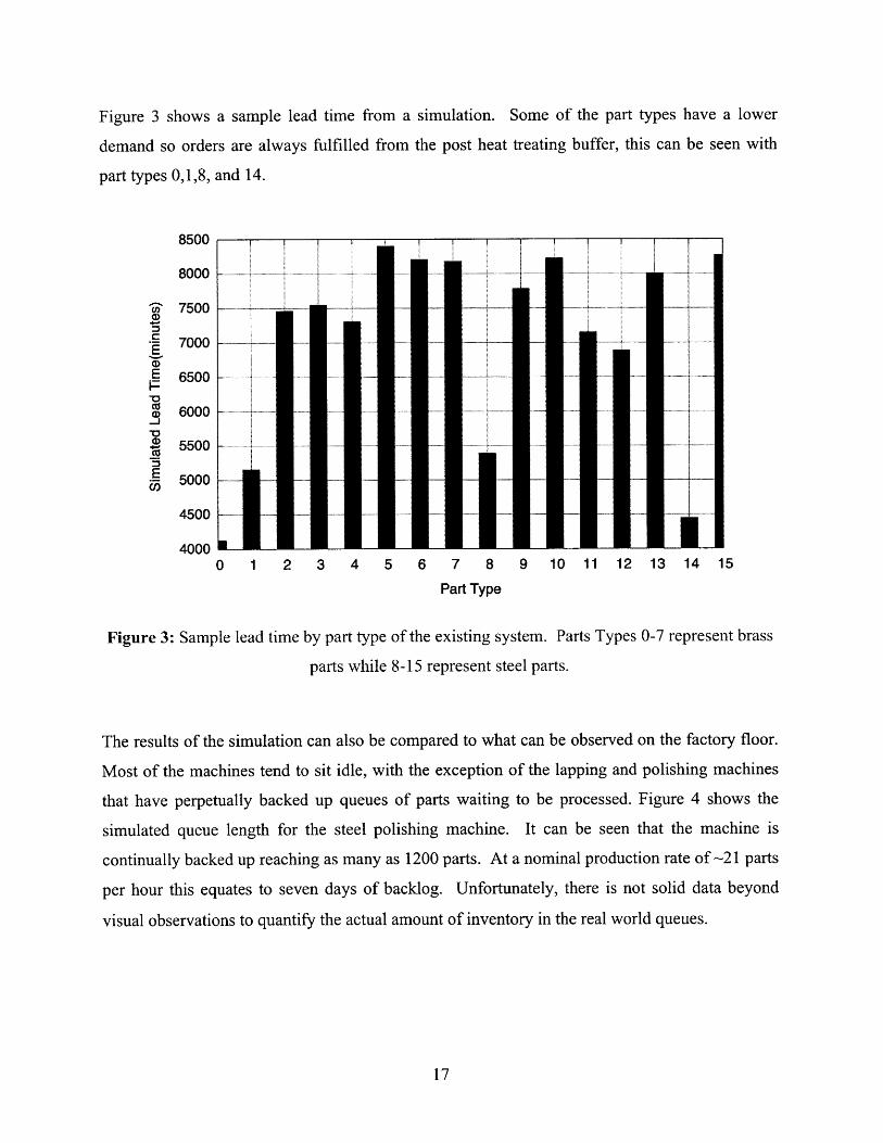
Figure 3 shows a sample lead time from a simulation. Some of the part types have a lower

demand so orders are always fulfilled from the post heat treating buffer, this can be seen with

part types 0,1,8, and 14.

0 1 2 3 4

I I I

•I

S-

5 6 7 8

Part Type

9 10 11 12 13 14 15

Figure 3: Sample lead time by part type of the existing system. Parts Types 0-7 represent brass

parts while 8-15 represent steel parts.

The results of the simulation can also be compared to what can be observed on the factory floor.

Most of the machines tend to sit idle, with the exception of the lapping and polishing machines

that have perpetually backed up queues of parts waiting to be processed. Figure 4 shows the

simulated queue length for the steel polishing machine. It can be seen that the machine is

continually backed up reaching as many as 1200 parts. At a nominal production rate of -21 parts

per hour this equates to seven days of backlog. Unfortunately, there is not solid data beyond

visual observations to quantify the actual amount of inventory in the real world queues.

17

8500

8000

7500

7000

6500

6000

5500

5000

4500

4000

1200

( 1000

0 800

o 600

4000

20 L

0 100000 200000 300000

Simulated Time(minutes)

Figure 4: Queue length of the steel polishing machine.

Chapter 4: Results

4.1 Existing System

The model was used to answer several hypothetical questions about the behavior of the

production system. The first question to answer was to determine the maximum theoretical

production rate of the existing system. Currently, Instron produces roughly 15,000 parts per

year. By increasing the demand rate of the simulation we are able to find the maximum

production rate to be about 24,000 parts per year. This is comparable to what is expected based

on the polishing rates from Table 1. When load/unload time is taken into account a simple hand

calculation indicates the polishing throughput should be around 26,000 parts per year. Figure 5

shows the total system output at a demand rate of 30,000 parts per year. Early on in the

simulation the system has still not reached a steady state, which is why the production rate is

initially erratic. Once the system reaches a steady state the production rate more or less

stabilizes. At peak output, when demand exceeds the production rate, it becomes clear that

polishing is the rate limiting process. The queue lengths for the steel and brass polishing

operations can be seen in Figure 6 and Figure 7, respectively. These queue lengths are growing

unbounded because the incoming arrival rate exceeds the production rate.

25000

20000

15000

10000

5000

100000 200000 300000

Time (minutes)

Figure 5: Production rate over time of the existing production system. Demand rate is 30,000

parts per year.

18000

16000

14000

12000

10000

8000

6000

4000

2000

0100000 200000 300000


Figure 6: Queue length for the steel polishing node at a demand rate of 30,000 parts per year.

. .

6000

5000

C 4000

n~ 3000 . . ...- __- --

2000E

1000

0 100000 200000 300000


Figure 7: Queue length for the brass polishing node at a demand rate of 30,000 parts per year.

4.2 Polishing Improvements

Mohammad Imani Nejad was able to improve the polishing process. The improvements allowed

the lapping stage to be completely removed, the processing time of the polishing machines to be

reduced from 15 minutes per 10 parts for both steel and brass to 4 minutes for steel and 1 minute

for brass. The rework rate was improved from nearly 50% to less than 5% [5]. Using these

modified rates the simulation predicts a peak output in excess of 40,000 parts per year given the

existing workforce of 4. Figure 8 shows the system output exceeding 40,000 parts per year with

a demand rate of 48,000 parts/year.

45000

40000

25000

0 20000

15000E

00 100000 200000 300000

Simulated Time (minutes)

Figure 8: Production rate over time with the proposed improvements to the polishing process.

Demand rate is 48,000 parts/year.

At 40,000 parts per year the polishing process is not a system bottleneck. Figure 9 shows the

average queue length for the brass polishing node at a demand rate of 48,000 parts per year. The

length of the queue is not growing overtime and never exceeds 140 parts. However, as shown in

Figure 10, the length of buffing node queue is growing unbounded which indicates that this node

is now the system bottleneck.

20

15

10

5

100000 200000 300000


Figure 9: Queue length over time for the bras polishing node at a demand rate of 48,000 partsper year.

14000

12000

10000

8000

6000

4000

2000

100000 200000 300000


Figure 10: Queue length over time for the grinding node at a demand rate of 48,000 parts peryear.

4.3 Maximizing Efficiency at Expected Demand Levels

While a peak throughput of 40,000 parts per year is a substantial increase over the initial peak

rate of just 24,000 parts per year, this production volume far exceeds excepted demand of

-20,000 parts per year. We are interested in maximizing the efficiency of the total system at

production levels slightly higher than the existing level of 15,000 parts per year. With Instron's

existing production setup, 4 workers are assigned to operate the 7 machines to meet the demand.

Instron is interested in minimizing the required workforce to meet existing and expected future

demand. Running the simulation with just one worker to service all machines we can validate

that it is in fact possible to do this. Figure 11 shows the production rate of the entire system with

one worker to operate all of the machines. It can be seen that the production rate tops out at

about 22,000 parts per year.

25000

20000

15000

10000

5000

0 100000 200000


300000

Figure 11: Production rate vs. time with proposed polishing improvements and a single workerwith a demand rate of 25,000 parts per year.

While the simulation is helpful to validate the concept of a single worker it is not feasible to

implement a single worker with current machine layout. With Instron's current setup, machines

are distributed throughout the large production facility at Binghamton despite the fact that most

of the machines used for the production of test blocks are dedicated to this task. It would be

ideal to consolidate all the machines required for production into a work-cell that can be easily

operated by one worker. The grinding and polishing machines do not need an operator while

running. However, it is important that the operator remain close to the machines in case there is

a problem.

A structured work schedule designed around a consolidated work-cell will address the

coordination issues associated with the single worker production. A full grinding cycle consists

of 15 minutes of setup, 2 hours of unattended operation, 30 minutes of cleaning and setup to turn

the parts over, 2 hours of operation, followed by 15 minutes of cleaning and removal for a total

cycle time of 5 hours. During a single 8 hour shift one full batch of 100 parts can be produced

on the grinder. If the grinder is run every other workday, 125 days per year, it can have an

annual throughput of 12,500 parts per year. 100 steel blocks every two days will be the takt time

for steel blocks. Historically, demand for brass blocks is slightly less than steel so it will have a

takt time of 80 parts every two days. This results in a total annual output of 22,500 parts per

year. Table 2 shows a proposed schedule to achieve the combined production rate of 22,500 parts

per year.

Table 2: Proposed production schedule for up to 22,500 parts per year with a single worker.

Parts ..9 .9 N N N N $4 P. 1 . 0 45

per Day i 8 & 8 8 A 8 i 8 A 8 i 8 A - 8 A 8 8 A 8 8 8Day 1:

Bead Blast Steel 105 VGrinding Steel 100Polishing Steel 100Polishing Brass 100Turning Brass 82.5Buffing Brass 83

Day 2:

Buffing Steel 100ATuring Steel 100

Machine Operating Unattended

. ................ - - - _ __ - 10..;; ; ; ; ; ;

With the proposed schedule on Day 1 the worker will remove 100 steel blocks from the existing

buffer of completed heat treated parts. It will take the worker 1:45 to buff all 100 blocks. After

buffing the worker will spend 15 minutes loading all 100 parts into the grinder. Once the grinder

is started he will simultaneously polish brass and steel blocks. It will take 1 hour to polish 100

steel and 100 brass blocks using the improved polishing procedure. Once polishing is finished

the worker will start turning and roll stamping brass blocks. While turning blocks, the worker

will have to spend 30 minutes reloading and cleaning the grinder so the second side of the blocks

can be ground. The next day, the worker will spend their day turning steel parts and buffing

brass parts to complete a full cycle of 100 steel blocks and 80 brass blocks.

This aggressive schedule demonstrates the limits of what is possible with the existing machinery.

If such an aggressive schedule were actually implemented several precautions would have to be

taken in order to ensure reliable production. Primarily, such a system relies on a continuous flow

of materials. All stages of the production process, except heat-treating, are performed in house

and can be closely controlled. Ensuring a continuous flow of parts from the heat-treater will

require close coordination and a carefully arranged supply agreement.

It was previously demonstrated that with a single worker and running at capacity the buffing

processes is the bottleneck of the system. As a result, the total system throughput is sensitive to

variations in this stage. If the rework rate triples from 5% to 15% the total system capacity is

reduced by nearly 20%. Figure 12 shows the system throughput with a 15% defect rate in the

buffing stage. The system is not as sensitive to increased rates of failure at other stages. Figure

13 shows the total system throughput with a 25% rework rate (nominally 5%) at the polishing

stage. Total system throughput is unchanged. The turning, bead blasting, and grinding stages

have less negative impacts.

25000

20000

15000

10000

5000

100000 200000 300000


Figure 12: System production rate with a 15% rework rate at the buffing stage.

25000

20000

15000

10000

5000

100000 200000 300000


Figure 13: System production rate with a 25% rework rate at the polishing stage.

WO

------- -

In addition to the degradation in throughput due to variations in the buffing stage, it was

recognized that nearly half of the worker's time is spent operating the CNC lathe during the

initial rough turning operation. Jairaj Vora has presented potential improvements to the rough

cutting and CNC turning processes that can reduce the worker's time spent operating the lathe.

Vora has proposed using a centerless grinder to turn the raw steel barstock to minimize the lathe

time spent turning parts to the final diameter. He has also proposed to add a bar-feeder to the

CNC lathe so it can be run unattended [8]. These two improvements have the potential to reduce

cycle times in the CNC lathe by as much as 50% and eliminate the need for the operator to

continuously tend to the machine. Figure 14 shows the effect of these improvements on the

simulated single worker production system. Peak throughput has been increased from 22,500 to

27,000 parts per year, a 20% improvement.

40000

35000

a 30000

S25000

1)08 20000 .. ....*. 15000E

5000

00 100000 200000 300000


Figure 14: Single worker production with proposed improvements to the initial turningprocesses.

Chapter 5: Conclusions and Recommendations

Using Python and freely available libraries, an accurate discrete event simulation model of

Instron's Rockewell hardness test block production line was created. This model was effective

at predicting the limits of Instron's existing production line. The model was also effectively used

to predict the overall production line performance when improvements are made to the polishing

process. Using the model the limits of the existing production system have been demonstrated.

The proposed improvements to the polishing process are shown to more than double the potential

production rate without any other improvements. The simulation model is a helpful tool for

predicting system behavior.

A production schedule and organization methodology, based on the findings uncovered by the

model, has been demonstrated to allow a single worker to produce over 20,000 parts per year. In

addition to reducing the required workforce, the proposed production method also reduces order

lead time. However, care should be taken when implementing such a system as it is shown to be

extremely sensitive to variations in the buffing stage.

Based on the results of the simulation it is clear that improving the polishing process and

eliminating the lapping stages provide substantial improvements in the overall system

throughput. Furthermore, the proposed production system, which utilizes these improvements,

allows a single worker to produce at levels exceeding current production volumes. When

implementing the production system it would be advisable to start at a lower production rate than

the peak capacity of 22,500 parts per year. If the grinder is operated every third day and the

other two days used to perform the other tasks an annual production rate of 15,000 parts per year

can be achieved. If higher production rates are desired, it has been shown that improvements to

the CNC turning process can allow annual production rates as high as 27,000 parts per year.

While working with the current production workers it became clear that when rework of

materials is required it is often unclear what process should be utilized to fix the defective parts.

As a result, workers tend to "pass the buck" to another production process. As a result excessive

rework often occurs, workers will send parts upstream to previous production processes

unnecessarily. By moving to a single worker responsible for all stages of production it is

plausible that the amount of unnecessary rework will be reduced as the individual worker will

have no where to "pass the buck."

As previously mentioned, the proposed production system is dependent on a continuous flow of

materials. Future work should investigate the sensitivity of the system to machine breakdowns,

heat treating delays, outsourced cutting delays, and stock out of raw materials.

It is apparent that tight coordination with the heat-treating supplier will be required.

Additionally, accurate demand forecasting will go a long way to ensure minimal lead times. A

standard inventory model, such as a base stock model, can be implemented to place orders into

the system in order to consistently produce the desired parts. Such an inventory model should be

used to control inventory across the entire product line and production facilities. With the

current setup, disjointed inventories are kept at the Binghamton and Norwood facilities. It seems

unnecessary to keep finished goods inventory at both locations. If these inventories can be

unified, total inventory volume can be further reduced.

Appendix A: Simulation Code

Usage:

Attached below is the Pythong code used to create the simulation used in this thesis. It was run using Python 2.5.1on MacOS 10.5.7. The following python libraries are also required:

SimPy 2.0.1Numpy 1.3.0Gnuplot.py 1.8

#python simulation.py [simulation duration] [data file name/path] [demand rate]

Usage Notes:* The demand rate argument is optional. If omitted the demand rate specified in the data file will be used.

* This script will create several output files in a folder called runs. Please create this folder before runningthe script. The files will be placed within runs in a new folder named with the current date and time.

* While running, the provide a continual system update to the user. Every time a new order is added to thesystem the time and number of parts in the system will be printed.

* If the demand rate substantially exceeds the production rate the number of parts in the system will growunbounded. On a 2.5ghz dual core CPU with 4GB of RAM systems with more than 25,000 parts run tooslow to be useful.

Code:

from SimPy.Simulation import *#from SimulationGUIDebug import *import random as ranimport shutil, csv, sys, Gnuplot, datetimeimport os as OSfrom SimPy.SimPlot import *from collections import dequefrom numpy import *import gc

execfile(sys.argv[2])random.seed(l)rate = int(sys.argv[3])

class Part(Process):def execute(self,i,pri,type,P,mean):

self.pri = pri;while i < len(mean):

global cpmon, compparts, st, myQ, wm, buffernode, outfile, inflight, sstock

if i == buffernode:if bufferdebt[type] == 0:

buffer[type]. append(self)

else:

ifi<> 1:

#printbuff()#print "buffer" + str(type) + ": " + str(len(buffer[type]))yield passivate, self

bufferdebt[type] -= 1#printbuff()

mqtime = now()yield request,self,mac[i],pri #queue for desiredw = workpool[i]mmon[i].observe(nowO-mqtime)wqtime = now()yield request,self,work[w],pri #queue for worker 1wmon[w].observe(nowO-wqtime)yield hold,self,loadtime[i]yield release,self,work[w] #release worker who loaded

if(len(myQ[i]) < maccap[i]-1):myQ[i].append(self);yield passivate, self

else:for x in myQ[i]:

reactivate(x);myQ[i]= [];

machine

to load into machine

#passivate if machine is not at capacity

#if machine is at capacity, activate all items in myQ

st[i] = ran.expovariate(1.0/mean[i])if needop[i]: #if node needs operator last part into node will q for

wqtime = now()yield request,self,work[w],priwmon[w].observe(nowo-wqtime)wm[i] = pri #wm[i] is the process holding operator

yield hold, self, st[i]

ifi <> 1:if (wm[i] = pri): #release worker if this was the holding process

yield release,self,work[w]wm[i] = None

wqtime = now()yield request,self,work[w],priwmon[w].observe(nowo-wqtime)yield hold,self,unloadtime[i]yield release,self,work[w]yield release,self,mac[i]

i = choose2dA(i,P) # choosecompparts += 1cpmon.observe(compparts* 120000/now())pendord[type][0]["num"] -= 1

inflight -= 1ifmon.observe(inflight-sstock)if pendord[type] [0] ["num"] == 0:

#print(str(now() - pendord[type][0]["start"]))pendord[type] [0]["end"]=now()

#unload part

next node to go to

pendord[type][0] ["tottime"]=now()-pendord[type] [0]["start"]compord[type].append(pendord[type] [0])#print "compord: "+ str(compord[type][-1]) + "\n\n\n"#printbuff()pendord[type] = pendord[type][1:]

def choose2dA(i,P): #from node i chooses next node j based on matrix PU = ran.randomosumP = 0.0for j in range(len(P[i])):

sumP += P[i][j]if U < sumP: break

return(j)

class Demand(Process):def execute(self,rate):

global outfile,os,types,buffernode,demparts,inflight,sstockself.count=0for i in types:

type = ifor j in range(0,os):

inflight +=1#ifmon.observe(inflight)self.count += 1p = Part(self.count)if type < matdiv:

P=Psmean = means

else:P = Pbmean = meanb

activate(p,p.execute(i=buffernode,pri=-self.count,type=type,P=P,mean=mean))sstock = inflight

while True:type = choose2dA(0,typedist)gc.collectOpendord[type].append( {"num":os,"size" :os,"start":now()})inflight += osifmon.observe(inflight-sstock)print str(nowO) + " : " + str(inflight)

demparts += osif now) > 10000:

rpmon.observe (demparts * 120000.0/now))for i in range(0,os):

self.count += 1p = Part(self.count)if type < matdiv:

P= Psmean = means

else:P = Pbmean = meanb

activate(p,p.execute(i=startMac,pri=-self.count,type=type,P=P,mean=mean))if len(buffer[type]) = 0:

bufferdebt[type] += 1else:

reactivate(buffer[type].pop())yield hold,self,ran.expovariate( 1.0/rate)

def printbuff():outfile = open("bufferfile","w")for type in types:

outfile.write(str(type) + ": start: "+ str(compord[type]["start"] + "\n"))outfile.closeo

initialize()inflight = 0sstock = inflight

buffer = {}bufferdebt = {}pendord = {}compord = {}leadtime = {}for type in types:

buffer[type]=[]bufferdebt[type]=0pendord[type]=[]compord[type]=[]leadtime[type]=[]

mac = []work = []

#register(Demand,name="Demand")wmon = {}mmon= { }ifmon = Monitor()cpmon = Monitor()rpmon = Monitor()

st = { } #st defines work time at each node, changes with each batch

myQ = [] #myQ keeps track of items waiting in machine before machine is fullwm = [] #wm keeps track of which process is holding the operatorcompparts = 0demparts = 0

for x in range(len(means)):myQ.append([]);wm.append([]);

for x in range(len(means)):mac.append(Resource(name="Machine%d"%x,capacity-maccap[x],qType=PriorityQ,monitored=True))#register(mac[x])mmon[x]=Monitor()

for x in range(len(workcap)):work.append(Resource(name="Worker%d"%x,capacity=workcap[x],qType=PriorityQ,monitored=True))#register(work[x])

wmon[x]=MonitorO

simendtime = float(sys.argv[1])g = Demand("Demand")activate(g,g.execute(rate))simulate(until=simendtime)print "done!"

leadtime = {}rowlist = ["type","leadtime"]ttimes = [1for type in types:

sum = 0for x in compord[type]:

sum += x["tottime"]ttimes.append(x["tottime"])

if len(compord[type]) =-- 0:leadtime[type] = 0

else:leadtime[type] = sum / len(compord[type])

dirname='runs/'+(str(datetime.datetime.utcnowo)[:- 5])+'/'OS.mkdir(dirname)shutil.copy(sys.argv[2],dirname+sys.argv[2])

print mean(ttimes)print std(ttimes)

def plotmonitor(mon,x,y,title,xtitle,ytitle,color-1):global dirnameif len(mon) == 0:

returnxl=[]yl = []for z in mon:

xl.append(z[x])yl .append(z[y])

g = Gnuplot.Gnuplotod = Gnuplot.Data(xl,yl, with='l It '+str(color))g('set grid')g.title(title)g.xlabel(xtitle)g.ylabel(ytitle)g.plot(d)g.hardcopy(filename=dirname+title+'.pdf,termina l= 'pdf)

drate = 200*2000*60/rateplotmonitor(ifmon,0,1,'Items in Flight: '+str(sys.argv[2]),'Time (minutes)','Items in Flight Minus Buffer Stock')plotmonitor(cpmon,0,1,'Production Rate vs Time ('+str(drate)+' pts yr)', 'Time (minutes)','Parts/Year')plotmonitor(rpmon,0,1,'Demand Rate vs Time ('+str(drate)+' pts per yr)', 'Time (minutes)','Parts/Year')

#macact = []#i = 0#total = 0#for x in mac:# if x[i] <> 0:

# macact[i] = x[i]# ifi o< 0:# total += macact[i][ l]# macact[i].append(total)# macact[i].append(total/macact[i][0])# else:# total = macact[i][1]# i += 1

#print macact[8]

i=0for x in mac:

if i <>l:plotmonitor(x.waitMon,0,1,'Machine '+str(i)+' Q Length','Simulation Time(minutes)','Items in Q')plotmonitor(x.actMon,0,1,'Machine '+str(i)+' Activity','Simulation Time(minutes)','Items in Q')

i+= 1

plotmonitor(work[1 ].waitMon,0, 1,'Worker'+str(i)+' Q Length','Simulation Time(minutes)','Items in Q')

g = Gnuplot.Gnuplot()d = Gnuplot.Data(leadtime.keyso,1eadtime.valueso, with='boxes fs solid It 1 lw .5 ')g('set grid')g.title('lead time by part type')g.ylabel('lead time (Simulation Minutes)')g.xlabel('part type')g.plot(d)g.hardcopy(filename=dimame+'leadtime.pdf,terminal='pdf)

Appendix B: Example Data File

from SimPy.Simulation import *#from SimulationGUIDebug import *import random as ran

types = range(0,16)typedist = [[ 0.05, 0.05, 0.05, 0.10, 0.10, 0.05, 0.05, 0.05, 0.05, 0.10, 0.10, 0.05, 0.05, 0.05, 0.05,0.05]]buffernode = 2matdiv = 7

#Overall Setupos = 200rate = 1600.0startMac = 0

#batch size#demand rate, overridden if specified at runtime#starting node

Ps = [[0.0, 1.0, 0.0, 0.0, 0.0, 0.0, 0.0, 0.0, 0.0, 0.0, 0.0],[0.0, 0.0,[0.0, 0.0,[0.0, 0.0,[0.0, 0.0,[0.0, 0.0,[0.0, 0.0,[0.0, 0.0,[0.0, 0.0,[0.0, 0.0,

1.0, 0.0, 0.0, 0.0, 0.0, 0.0, 0.0, 0.0, 0.0],0.0, 1.0, 1.0, 0.0, 0.0, 0.0, 0.0, 0.0, 0.0],0.0, 0.0, 1.0, 0.0, 0.0, 0.0, 0.0, 0.0, 0.0],0.0, 0.0, 0.0, 1.0, 0.0, 0.0, 0.0, 0.0, 0.0],0.0, 0.0, 0.0,0.05, 0.0,0.95, 0.0, 0.0, 0.0],0.0, 0.0, 0.0, 0.0, 0.0, 0.0, 0.0, 0.0, 0.0],0.0, 0.0, 0.0, 0.0, 0.0, 0.2, 0.0, 0.8, 0.0],0.0, 0.0, 0.0, 0.0, 0.0, 0.0, 0.0, 0.0, 0.0],0.0, , 0.0 , 0.0, 0.0, 0.3, 0.0, 0.5, 0.2]]

Pb = [[0.0, 1.0, 0.0, 0.0, 0.0, 0.0, 0.0, 0.0, 0.0, 0.0, 0.0],[0.0, 0.0, 1.0, 0.0, 0.0, 0.0, 0.0, 0.0, 0.0, 0.0, 0.0],[0.0, 0.0, 0.0, 0.0, 0.0, 1.0, 0.0, 0.0, 0.0, 0.0, 0.0],[0.0, 0.0, 0.0, 0.0, 0.0, 0.0, 0.0, 0.0, 0.0, 0.0, 0.0],[0.0, 0.0, 0.0, 0.0, 0.0, 0.0, 0.0, 0.0, 0.0, 0.0, 0.0],[0.0, 0.0, 0.0, 0.0, 0.0,0.05,0.95, 0.0, 0.0, 0.0, 0.0],[0.0, 0.0, 0.0, 0.0, 0.0, 0.0, 0.2, 0.0, 0.8, 0.0, 0.0],[0.0, 0.0, 0.0, 0.0, 0.0, 0.0, 0.0, 0.0, 0.0, 0.0, 0.0],[0.0, 0.0, 0.0, 0.0, 0.0, 0.0, 0.3, 0.0, 0.5, 0.0, 0.2],[0.0, 0.0, 0.0, 0.0, 0.0, 0.0, 0.0, 0.0, 0.0, 0.0, 0.0]]

#machine setupmeans = [2.6, 3600, 0.0001,40.0, 240.0, 1.8, 0.0, 10.0, 0.0, 15.0]processing time per batch each nodemeanb = [1.6, 3600, 0.0001, 0.0, 0.0, 0.7, 10.0, 0.0, 15.0, 0.0]processing time per batch each node

#mean

#mean

loadtime = [ .1, 0, 0.0001, 0.1, 0.14, 0.01, 0.2, 0.2, 0.2, 0.2]each nodeunloadtime = [ .1, 0, 0.0001, 0.1, 0.6, 0.01, 0.2, 0.2, 0.2, 0.2]each nodemaccap = [ 1, os, 1, 50, 100, 1, 20, 20, 10, 10]

#load time per part at

#load time per part at

#machine capacity

#worker setupworkpool =needop =is requiredworkcap =worker pool

[1,0,0,2,2,2,3,3,4,4][1,0,0,1,0,1,1,0,0]

[99999,1,1,1,1]

#which worker pool is needed at node i#boolean to define if a continuous operator

#number of workers available in each

Appendix C: Variables

Variable

types

typedist

buffernode

matdiv

os

rate

startMac

Ps

Pb

means

meanb

loadtime

unloadtime

maccap

workpool

needop

workcap

Type

int range

vector double

int

int

int

double

int

matrix double

matrix double

vector double

vector double

vector double

vector double

vector int

vector int

vector bool

vector int

Description

total number of part types

probability of demand for each part type

node of buffer

number of brass part types

number of parts in 1 order

demand rate, can be overridden at runtime

first node of the system

transition matrix for steel parts

transition matrix for brass parts

mean processing time for steel

mean processing time for brass

loading time for each machine

unloading time for each machine

machine capacity

which worker group is assinged to each machine

weather a machine needs an operator while running

the number of workers in each group

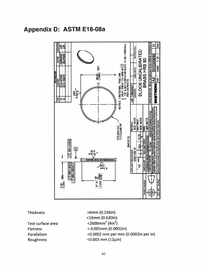
Appendix D: ASTM E18-08a

Thickness

Test surface areaFlatnessParallelismRoughness

>6mm (0.236in)<16mm (0.630in)<2600m 2 (4in2 )< 0.005mm (0.0002in)<0.0002 mm per mm (0.0002in per in)<0.003 mm (121 in)

References1. Khoshnevis, B. (1994). Discrete Systems Simulation. New York: McGraw-Hill.

2. Law, A. M., & Kelton, W. D. (1991). Simulation Modeling and Analysis. New York:McGraw-Hill.

3. Law, A. M., & McComas, M. G. (2001). How to Build Valid and Credible SimulationModels. Proceedings of the 2001 Winter Simulation Conference (p. 8). Tuscon, AZ: AverillM. Law and Associates, Inc.

4. Matloff, N. (2008). Advanced Features of the SimPy Language. Davis, CA.

5. Nejad, M. I. (2009). Improving the Polishing Process for Rockwell Hardness. Cambridge:MIT.

6. SimPy Developer Team. (2009). SimPy Homepage. Retrieved 8 1, 2009, fromhttp://simpy.sourceforge.net/

7. Tan, V. (2009). Heat treatment optimization in the manufacture of Wilson Rockwell SteelHardness Test Blocks. Cambridge: MIT.

8. Vora, J. (2009). Variations in the Manufacturing ofRockwell Test Blocks. Cambridge: MIT.

Discrete Event Simulation and Production System Design for ...

Documents

Transcript of Discrete Event Simulation and Production System Design for ...