Discrete Choice Model Analysis of Mobile Telephone ...ida/3Kenkyuu/4ouyoumicro/2005ou...2 Discrete...

1

Discrete Choice Model Analysis

of Mobile Telephone Service Demand in Japan

Takanori Ida

Graduate School of Economics, Kyoto University

Yoshida, Sakyoku, Kyoto 606-8501, Japan

and

Toshifumi Kuroda



Correspondence:

Takanori Ida



Tel & Fax: +81- 75-753-3477

E-mail: [email protected]

2

Discrete Choice Model Analysis

of Mobile Telephone Service Demand in Japan

Abstract:

The Japanese mobile telephone industry is now moving from second generation (2G)

standards to third generation (3G) standards. This paper analyzes the demand for mobile

telephones including 2G and 3G by using a discrete choice model called a mixed logit

model. First, we examine the substitution patterns of the demand for mobile telephones

and show that demand substitutability among alternatives is stronger within the provider

nest category than within the standard nest category in mobile telephone services. The

closest substitute for NTT’s 3G service is NTT’s 2G service, rather than KDDI’s 3G

service, for example. Second, we investigate the elasticities of demand for various

functions including e-mail, Web browsing, and moving-picture delivery. Consequently,

we cannot observe marked differences between 2G and 3G services based on these

calculated elasticities, indicating that it takes time for 3G subscribers to gain proficiency

with such new services.

Running title: mobile telephone service in Japan

JEL classifications: L52; L86; L96

Keywords: discrete choice model, mixed logit model, mobile telephone, cellular phone,

IMT 2000

3

1. Introduction

As of September of 2004, the number of Japanese mobile telephone subscribers reached

84 million, easily surpassing the 60 million fixed telephone subscribers. Mobile Internet

service started in February 1999, and third generation (3G) mobile telephone services

appeared on the market in October 2001, both of which were the first such introductions

in the world. Furthermore, mobile telephone functions have remarkably diversified from

simple voice and data transmissions to built-in camera phones, financial transactions,

and TV and radio reception. The purpose of this paper is to investigate this rapidly

evolving demand for mobile telephone services including 3G services by using a

discrete choice model called a mixed logit model.

First, we quickly review the related literature. Few papers have studied demand for

mobile telephone services, as pointed out by Taylor (2002 p.130). Research into

demand for 3G services is even less common. An exception is Kim (2005), who

investigated consumer stated preferences for 3G services (IMT 2000) in Korea by using

conjoint analysis. Other important papers on demand for mobile telephone services

include the following. The first studies are cross-country research. Ahn and Lee (1999)

compared the subscriber rates of mobile telephone services in developed countries and

found that income is a more important attribute than charges. Wallsten (2001) explored

the effects of privatization, competition, and regulation on mobile operator performance

in 30 African and Latin American countries, and Madden et al. (2004) estimated

elasticities of demand for mobile telephone service with respect to price and income,

based on panel data from 56 countries. Liikanen et al. (2004) analyzed the role of

generational effects in diffusion, interestingly finding positive within-generation

network effects.

The second are cases from individual countries. Ahn (2001) estimated the access

demand for mobile telephone service in Korea and found that age, gender, and

education are important determinants. Tishler et al. (2001) and Kim and Kwon (2003)

analyzed mobile telephone demand by using the multinomial logit model: the former

treated projections for the Israeli mobile telephone market up to 2008, while the latter

discussed the advantages of network size in acquiring new subscribers in the Korean

mobile telephone market. Finally, Iimi (2005) analyzed the Japanese mobile telephone

service industry from quite a different angle than this paper, concluding that the market

4

is highly product-differentiated and no longer displays conventional network

externalities.

This paper analyzes the access demand for Japanese mobile telephone services by

using a discrete choice model. It makes two contributions. The first is the research

object. This paper analyzes consumers’ revealed preferences regarding mobile

telephone subscriptions with a special emphasis on the differences between 2G and 3G

services. This is one of the first studies that explicitly deal with 3G service. The second

is the research method. To analyze decision-making structures in Japan’s mobile

telephone market, we need to relax the independence from irrelevant alternatives (IIA)

properties imposed on conditional logit (CL) models. We adopt a mixed logit (ML)

model that can flexibly express an analog to overlapping nested structure, which is a

recently developed econometric innovation.

The two main conclusions obtained in this paper are summarized as follows. First,

we investigate substitution patterns in mobile telephone services and conclude that

demand substitutability among alternatives is stronger within the provider nest category

than within the standard nest category. The 1% increase in the basic monthly charge of

NTT’s 3G service (called FOMA) decreases its choice probability by 0.8%. At the same

time, this increases the probability of choosing NTT’s 2G service (called MOVA) by

0.5% but the probability of choosing KDDI’s 3G service (called CDMA 2000) only by

0.1%. We thus see that the closest substitute for NTT’s 3G service is NTT’s 2G service,

rather than KDDI’s 3G service. The same thing can be said of NTT’s 2G service. These

conclusions demonstrate that many mobile telephone subscribers apparently feel locked

in to their current providers because the costs of switching providers are quite high,

especially considering e-mail addresses and various discount services (family

membership and long-term contracts).

Next, we analyze the elasticities of demand for various functions. Looking at

explanatory variables whose t-values are statistically significant, including e-mail, Web

browsing, moving-picture delivery, we cannot confirm that the elasticities of demand

are clearly different between 2G and 3G services. A possible reason is a changeover

from 2G to 3G services is happening at this moment, and even successful 3G

subscribers fail to display outstanding utilization that differs from existing 2G services.

However, it would be hasty to conclude that 3G service is no more than 2G service in

terms of functional utilization because there is a time lag between starting to use a new

5

service and getting used to it.

This paper is organized as follows. Section 2 introduces sample surveys and the data.

Section 3 explains the estimation model and examines the advantages of the ML model.

Section 4 analyzes the estimation results, looking closely into the elasticities of demand

with respect to price and functions. Finally, Section 5 provides concluding remarks.

2. Survey Method and Data

This section introduces the survey and data used in this paper. We carried out sample

surveys on individual usage of mobile telephones and PHS in September 2004 jointly

with the Japanese Ministry of Internal Affairs and Communication (MIC). The survey

was conducted on 1000 monitors 20 years old and over who were registered with eleven

local offices of MIC. The number of respondents was 939. Among them, 764 people

(81.4%) subscribe to a mobile telephone or PHS. Excluding omissions, we finally

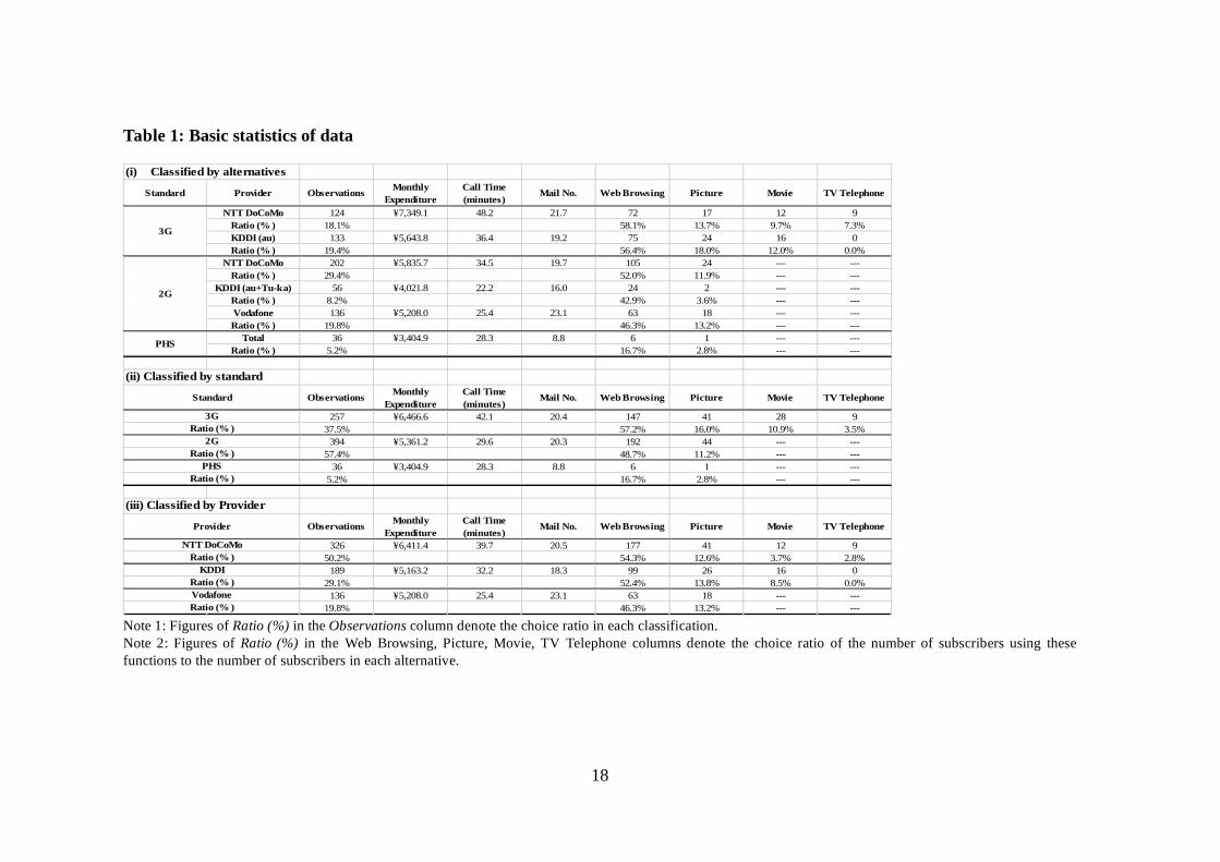
obtained 687 effective respondents whose breakdown is given in Table 1 according to

technical standards (i.e., 2G, 3G, and PHS) and providers (i.e., NTT DoCoMo, KDDI

(au and Tu-ka), and Vodafone).

<Table 1: Basic statistics of data >

The choice ratios were broken down into 3G (37.5%), 2G (57.4%), and PHS (5.2%)

according to technical standards. Compared to actual market shares, the 3G choice

ratios are higher in our survey, which reflects that the monitors registered with the

survey are more interested in telecommunications services than the average Japanese

person1. Also, by provider the choice ratio breakdowns into NTT (50.2%), KDDI

(29.1%), and Vodafone (19.8%). Compared to actual market shares, NTT’s choice ratio

is lower in our survey, which is in part based on the fact that the 3G choice ratio is

higher in our sample survey and that NTT’s share is not so high in the 3G market

2.

Let us now examine the details. Monthly Expenditure includes basic monthly

1 MIC reported that the actual market shares were 3G (27.1%), 2G (67.6%), and PHS

(5.3%) as of September 2004. 2 MIC reported that the actual market shares were NTT (56.1%), KDDI (26.0%), and

Vodafone (17.9%) as of September 2004.

6

charges, additional function charges, call charges, and packet-switched data

transmission charges3. 3G service is more expensive than 2G and PHS services, and the

monthly expenditures of NTT are also more expensive than KDDI and Vodafone. Call

Time indicates minutes called per week. 3G service accumulates more minutes than 2G

and PHS services, and NTT’s also accumulates more call time than KDDI and

Vodafone. Mail No. indicates the number of sent/received e-mails per week. Note that

87.7% of mobile telephone subscribers who replied said that they use e-mail services by

mobile telephone. There is no big difference between 2G and 3G services while PHS’s

mail number is much smaller, and Vodafone subscribers use e-mail services more

frequently than NTT and KDDI subscribers. Web Browsing represents the number of

users who replied that they frequently use Web browsing services by mobile telephone.

49.3% of mobile telephone subscribers frequently use Web browsing services. 3G

service ranks first, followed by 2G service and then PHS service; NTT also leads KDDI

and Vodafone in Web browsing. Picture represents the number of users who replied

that they frequently use still-picture delivery services by mobile telephone. 12.5% of

mobile telephone subscribers frequently use still-picture delivery services. 3G service

ranks first, followed by 2G service and PHS service, and KDDI also slightly leads

Vodafone and NTT in picture delivery service. Movie represents the number of users

who frequently use moving-picture delivery services by mobile telephone. This service

is basically provided by 3G services, and only 10.9% of 3G subscribers frequently use

moving-picture delivery services. Only 3.5% of 3G subscribers use TV telephone

services. The last two facts demonstrate that 3G high-speed data transmission services

have not yet been fully utilized.

3. Econometric Model

This section explains econometric models. In this paper, we analyze mobile telephone

service demand by using a discrete choice model. Conditional Logit (CL) models that

assume independent and identical distribution (IID) of random terms have been widely

used. However, independence from the irrelevant alternatives (IIA) property derived

3 Figures represent amounts subtracted by various discount services and do not include

toll information service charges.

7

from the IID assumption of the CL model is too strict to allow for flexible substitution

patterns. A nested logit (NL) model partitions the choice set to allow alternatives to

share common unobserved components among one another compared with non-nested

alternatives by partially relaxing strong IID assumptions. However, even the NL model

is not suited for our analysis because it is becoming too arbitrary to determine the nested

structure, and we have no information about which factor mobile telephone subscribers

emphasize, technical standard or provider brand. Naturally, both are important factors

for mobile telephone subscribers. In such cases, we have to express an overlapping

nested structure composed of both technical standard and provider brand. Consequently,

the most prominent model is a mixed logit (ML) model that accommodates differences

in covariance of the random components (or unobserved heterogeneity). ML models are

highly flexible to obviate the limitations of the CL model by allowing for random taste

variation, unrestricted substitution patterns including overlapping nested structure, and

the correlation of random terms over time (see McFadden and Train 2000, Ben-Akiva,

Bolduc, and Walker 2001 for details).

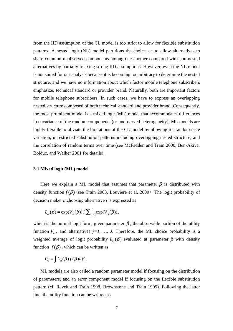
3.1 Mixed logit (ML) model

Here we explain a ML model that assumes that parameter is distributed with

density function ( )f see Train 2003, Louviere et al. 2000 . The logit probability of

decision maker n choosing alternative i is expressed as

L

ni( ) = exp(V

ni( )) / exp(V

nj( ))

j=1

J

,

which is the normal logit form, given parameter , the observable portion of the utility

function niV , and alternatives j=1, …, J. Therefore, the ML choice probability is a

weighted average of logit probability ( )niL evaluated at parameter with density

function ( )f , which can be written as

( ) ( )ni niP L f d= .

ML models are also called a random parameter model if focusing on the distribution

of parameters, and an error component model if focusing on the flexible substitution

pattern (cf. Revelt and Train 1998, Brownstone and Train 1999). Following the latter

line, the utility function can be written as

8

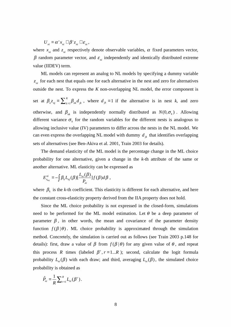
U

ni= ' x

ni+ ' z

ni+

ni,

where x

ni and

z

ni respectively denote observable variables, fixed parameters vector,

random parameter vector, and ni

independently and identically distributed extreme

value (IIDEV) term.

ML models can represent an analog to NL models by specifying a dummy variable

z

ni for each nest that equals one for each alternative in the nest and zero for alternatives

outside the nest. To express the K non-overlapping NL model, the error component is

set at n

znj

=nk

djkk =1

K

, where 1jkd = if the alternative is in nest k, and zero

otherwise, and nk

is independently normally distributed as (0, )kN . Allowing

different variance k for the random variables for the different nests is analogous to

allowing inclusive value (IV) parameters to differ across the nests in the NL model. We

can even express the overlapping NL model with dummy jkd that identifies overlapping

sets of alternatives (see Ben-Akiva et al. 2001, Train 2003 for details).

The demand elasticity of the ML model is the percentage change in the ML choice

probability for one alternative, given a change in the k-th attribute of the same or

another alternative. ML elasticity can be expressed as

( )( )[ ] ( )

knj

ni nix k nj

ni

LE L f d

P= ,

where k is the k-th coefficient. This elasticity is different for each alternative, and here

the constant cross-elasticity property derived from the IIA property does not hold.

Since the ML choice probability is not expressed in the closed-form, simulations

need to be performed for the ML model estimation. Let be a deep parameter of

parameter , in other words, the mean and covariance of the parameter density

function ( | )f . ML choice probability is approximated through the simulation

method. Concretely, the simulation is carried out as follows (see Train 2003 p.148 for

details): first, draw a value of from ( | )f for any given value of , and repeat

this process R times (labeled , 1...r r R= ); second, calculate the logit formula

probability ( )niL with each draw; and third, averaging ( )niL , the simulated choice

probability is obtained as

1

1ˆ ( )R r

ni nirP L

R == .

9

This simulated choice probability ˆniP is an unbiased estimator of niP whose

variance decreases as R increases. The simulated log likelihood (SLL) function is given

as

1 1

ˆlnN J

nj nin jSLL d P

= == ,

where 1njd = if decision maker n chooses alternative j, and zero otherwise. The

maximum simulated likelihood (MSL) estimator is the value of that maximizes this

SLL function.

In what follows, we adopt the ML model for the estimation, place dummy variables

for 2G and 3G users and for NTT and KDDI users, respectively, and intersect these

dummy variables with random parameters. Accordingly, we can express an analog to

the overlapping nested structure of decision making in mobile telephone services. We

then use the MSL method for estimation by setting 100 time random draws4 5.

3.2 Variables

Here we explain the explained and explanatory variables in our model. First, the

explained variables are the following six alternatives6:

NTT’s 3G

4 Louviere et al. (2000 p. 201) suggest that 100 replications are normally sufficient for a

typical problem involving five alternatives, 1000 observations, and up to 10 attributes

(see also Revelt and Train 1998), although the number of random draws is still an issue

of controversy. 5 The adoption of other draw methods including Halton sequence draw is an important

problem to be examined in the future (see Halton 1960). Bhat (2001) found that 100

Halton sequence draws are more efficient than 1000 random draws for simulating a ML

model. However, an anomaly may arise in this analysis, and therefore the properties of

Halton sequence draws in simulation-based estimation needs to be investigated further

(see Bhat 2001, Train 2003). As a matter of fact, we could not obtain stable estimation

results using Halton sequence draw, whereas the results were quite stable when using

random draws. This is why we adopt random draw for our analysis. Determining the

suited draw method is still open for future research. 6 McFadden (1984) claimed that it is difficult to obtain reliable estimations for an

alternative that has less than 30 samples. Therefore, we deleted Vodafone’s 3G service

from the choice set, integrated au’s 2G service and Tu-Ka’s service into KDDI’ 2G

service, and considered various PHS services as one brand.

10

KDDI’s 3G

NTT’s 2G

KDDI’s 2G

Vodafone’s 2G

PHS

Next, explanatory variables are set as follows:

Constant: Dummy variables are put on 2G, 3G, NTT, and KDDI users. As such,

for example, the constant term for NTT’s 3G is expressed as the sum of the 3G

dummy coefficient and the NTT dummy coefficient.

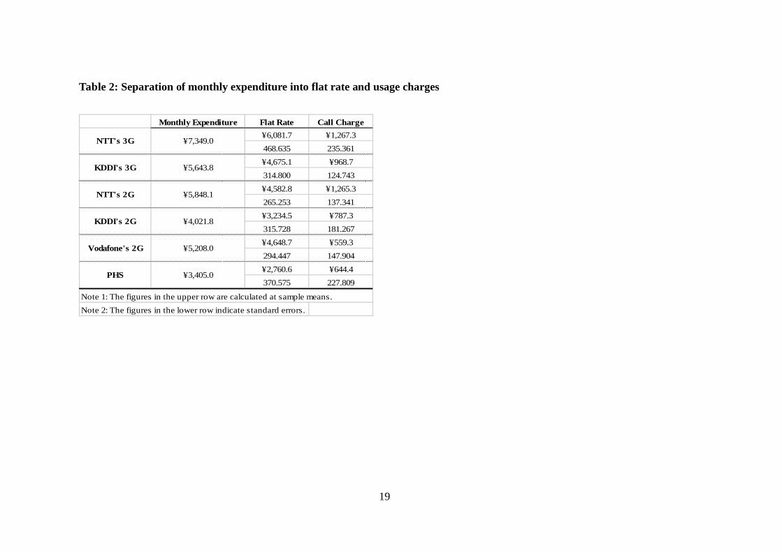
Flat Rate: Monthly Expenditures in Table 1 are composed of monthly flat

charges and usage charges that increase with call time. Therefore, monthly

expenditure is not a proper explanatory variable because it is endogenously

determined by other explanatory variables such as call time: an increase in call

time increases monthly expenditures. At this point, we adopt the following

strategy to avoid this problem: we first regress Monthly Expenditure on Call

Time and other variables including Mail No., Web Browsing, Picture, and

Movie, and, second, separate the monthly expenditure into flat rate and usage

rate parts. Following Kim (2005), we define flat rate independent of call time as

a basic price variable7 8. Table 2 depicts the separation of monthly expenditure

into flat rate and usage charges9.

Call Time: calling minutes per week.

Mail No.: number of sent/received e-mails per week.

Web: dummy variable for an individual who often uses Web browsing services.

Picture: dummy variable for an individual who often uses still-picture delivery

7 Since discrete choice models are normally concerned with the analysis of access

demand, the flat rate part is considered a basic price variable where a tariff structure

takes the form of a complicated multipart system (see Train 2003, for example). 8 Strictly speaking, we should have extracted the usage rate charge that depends on data

transmission from the flat rate charge. However, we do not exclude the data

transmission charge from the flat rate charge because the flat rate system for data

transmission has significantly penetrated Japanese mobile telephone services. 9 Note that all flat rate and usage charge estimates are statistically significant at the 1% level according to t-values.

11

services.

Movie: dummy variable for an individual who often uses the moving-picture

delivery service.

<Table 2: Separation of monthly expenditure into flat rate and usage charges >

For parameters, the utilities derived from various functions are likely to differ

between the 2G and 3G services because their qualities of service are different.

Therefore, we estimate different parameters for technical standards. Furthermore, such

explanatory variables as Call Time, Mail No., Web, Picture, and Movie are so-called

individual characteristics. Since only the differences of utility parameters between two

alternatives matter in the discrete choice model analysis, we actually measure the

influences of individual characteristics on the choice probabilities of the 2G and 3G

alternatives on the basis of the PHS alternative (see Greene 2003 for details). For

example, parameter Call Time 3G represents an incremental utility of choosing the 3G

alternative compared to the PHS alternative10

.

4. Estimation results

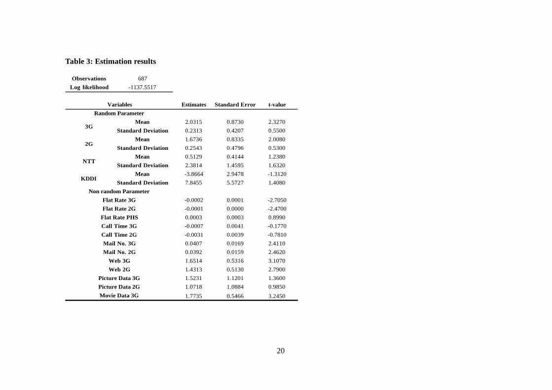
This section discusses the estimation results of the ML model. Results are given in

Table 311

. First, we see that Constants (means of 2G and 3G), Flat Rate (2G, 3G), Mail

(2G, 3G), Web (2G, 3G), and Movie (2G, 3G) are statistically significant at the 5%

level, according to the t-values. Assuming that parameters for 2G, 3G, NTT, and KDDI

dummies are normally distributed, correlations between alternatives are allowed here.

The values of standard deviations of random parameters are not statistically significant

except that NTT is statistically significant at the 10% level12

. However, the IIA property

10 Note that for this reason parameters such as Call Time PHS, Mail No., PHS, and so on do not appear explicitly in Table 3. 11 Before moving to the ML model estimation, we carried out ordinary CL model

estimation and confirmed that the IIA property is rejected at the 1% statistically

significant level because the value of Hausman test statistic is 48.24 when we excluded

KDDI’s 2G alternative. 12 Since the IIA property has already been rejected, we should not return to a

non-random parameter CL model.

12

is completely relaxed in the ML model so that flexible substitution patterns can be

expressed. One power of the ML model can be seen in that cross elasticities of demand

are all different, which will be discussed in the next subsection.

<Table 3: Estimation results>

4.1 Price elasticities

We here investigate the elasticities of access demand (choice probability) with

respect to monthly flat rate price (hereafter price elasticities). There are two kinds of

price elasticities. The first is own (or direct) elasticity, which measures the percentage

change in the choice probability with respect to a given percentage change in the price

of the same alternative. The second is cross elasticity, which measures the percentage

change in the choice probability with respect to a given percentage change in the price

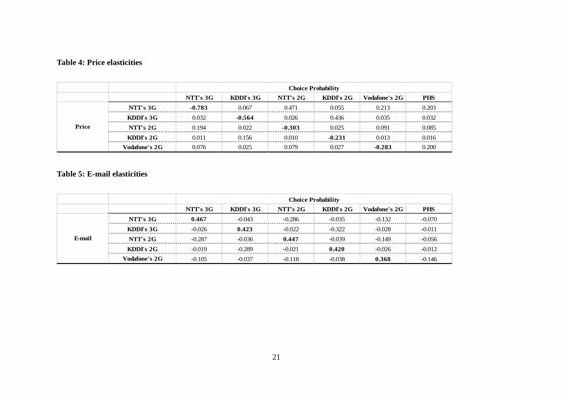
of another alternative. Calculation results are indicated in Table 4.

<Table 4: Price elasticities>

Looking at the first row, with respect to NTT’s 3G price, the own elasticity of

NTT’s 3G is -0.783, and cross elasticities are 0.067 for KDDI’s 3G, 0.471 for NTT’s

2G, 0.055 for KDDI’s 2G, 0.213 for KDDI’s 2G, and 0.203 for PHS. Note that cross

elasticities vary across alternatives because the IID assumption is completely relaxed

here.

Let us go into the details. The 1% decrease in NTT’s 3G flat rate price increases the

probability of choosing NTT’s 3G by 0.8%. At the same time, this price change

decreases the probability of choosing NTT’s 2G by 0.5%, while decreasing the

probability of KDDI’s 3G by only 0.1%. The closest substitute for NTT’s 3G is not

KDDI’s 3G but NTT’s 2G. Similarly, the 1% decrease in NTT’s 2G flat rate price

increases the probability of choosing NTT’s 2G by 0.3%. At the same time, this price

change decreases the probability of choosing NTT’s 3G by 0.2%, while hardly affecting

the probability of KDDI’s 2G and decreasing the probability of choosing Vodafone’s

2G by only 0.1%. The closest substitute for NTT’s 2G is neither KDDI’s 2G nor

Vodafone’s 2G but NTT’s 3G. The same thing applies to KDDI’s 3G and 2G.

13

Consequently, the demand substitutability of mobile telephone services works not

within technical-standard categories but within the provider-brand categories. A

possible reason is that subscribers tend to be locked in to their current providers through

switching costs caused by telephone numbers, e-mail addresses, family-member

discount services, long-term discount services, and so on13

.

Next, we compare the total price elasticities according to technical standards

(namely, 2G and 3G). The total price elasticities of 3G services can be derived in the

following way (see Motta 2003, pp.125-126)14

. Suppose that the prices of NTT’s 3G

and KDDI’s 3G services increase independently and simultaneously by 1%; the

probability of choosing NTT’s 3G decreases by 0.783% with a 1% increase in NTT’s

3G price but increases by 0.032% with a 1% increase in KDDI’s 3G price; in sum, the

total price elasticity of NTT’s 3G is 0.751. In the same way, the total price elasticity of

KDDI’s 3G is 0.497. Turning to the total price elasticities of 2G services, the values are

0.214 for NTT’S 2G, 0.179 for KDDI’s 2G, and 0.179 for Vodafone’s 2G. It follows

that 3G services are more price-sensitive than 2G services based on total price

elasticities. In other words, the probability of choosing 3G services changes more

sensitively than 2G services for percent changes in prices.

4.2 Other elasticities

We then refer to other elasticities with respect to various functions including e-mail,

Web browsing, and moving-picture delivery that are statistically significant variables.

Table 5 indicates the demand elasticities for the number of e-mails per week. There

is only a small difference between NTT’s 3G and NTT’s 2G and between KDDI’s 3G

and KDDI’s 2G for e-mail own-elasticities. This is probably because 3G services do

have an advantage over 2G services for simple text message service.

<Table 5: E-mail elasticities>

13 Note that MIC has determined to introduce a number portability system into the Japanese mobile telephone market from 2006 to encourage competition. 14 McFadden (1979) suggests an aggregation rule of elasticities over plural alternatives

and variables.

14

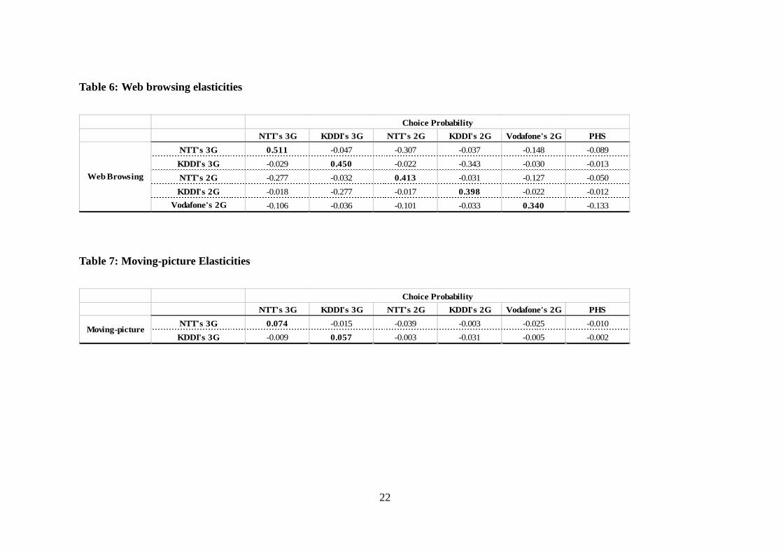
Table 6 indicates demand elasticities with respect to the frequent use of Web

browsing services. The figures are about 0.5 for 3G services and about 0.4 for 2G

services; the Web-browsing elasticities are a little larger for 3G services than for 2G

services, reflecting that Web browsing requires larger volume data transmission, and 3G

service has an advantage over 2G service in this respect, although the difference of

elasticities is still small.

<Table 6: Web browsing elasticities>

Last, Table 7 indicates the demand elasticities of the frequent use of moving-picture

delivery services. The figures of the elasticities are less than 0.1 for 3G services.

Although moving-picture delivery service is statistically significant, its positive impact

on the probability of choosing 3G services is quite small. Although a moving-picture

delivery service that requires high-speed, large-volume data transmission is thought to

be a “killer application” for further diffusion of 3G services, it has not yet been fully

utilized by 3G subscribers.

<Table 7: Moving-picture elasticities>

In conclusion, after examining demand elasticities for various functions including

e-mail, Web browsing, and moving-picture delivery, we failed to observe remarkable

differences between 2G and 3G services. Perhaps a changeover is now occurring from

2G services to 3G, while even progressive 3G subscribers fail to make full use of new

3G services.

5. Conclusion

This paper investigated the demand for mobile telephone services including 3G. We

particularly focused on the demand substitutability between mature 2G services and

emerging 3G services. Two main conclusions are obtained. First, there is a clear

distinction between 2G and 3G services for values of price elasticity. 3G services are

more price-elastic than 2G services. This conclusion demonstrates that 3G service is

still in the process of full-scale diffusion, and new 3G subscribers are currently more

15

sensitive to price changes than 2G subscribers. Second, turning to the analysis of

functions such as e-mail, Web browsing, and moving-picture delivery, we failed to

discover distinct evidence to show that 3G subscribers make full use of new 3G services.

However, since the development of mobile telephone services is remarkable, we should

carefully observe the evolution from now on.

16

References

Ahn, H. and Lee, M.H. (1999) "An Econometric Analysis of the Demand for Access to

Mobile Telephone Networks," Information Economics and Policy 11: 297-305.

Ahn, H. (2001) "A Nonparametric Method of Estimating the Demand for Mobile

Telephone Networks: An Application to the Korean Mobile Telephone Market,"

Information Economics and Policy 13: 95-106.

Bhat, C. (2001) "Quasi-random Maximum Simulated Likelihood Estimation of the

Mixed Multinomial Logit Model," Transportation Research B 35: 677-693.

Ben-Akiva, M., Bolduc, D., and Walker, J. (2001) "Specification, Estimation and

Identification of the Logit Kernel (or Continuous Mixed Logit) Model,"

Working Paper, Department of Civil Engineering, MIT.

Brownstone, D. and Train, K.E. (1999) "Forecasting New Product Penetration with

Flexible Substitution Patterns," Journal of Econometrics 89: 109-129.

Greene, W.H. (2003) Econometric Analysis (5th), Prentice Hall.

Halton, J. (1960) "On the Efficiency of Evaluating Certain Quasi-random Sequences of

Points in Evaluating Multi-dimensional Integrals," Numerische Mathematik 2:

84-90.

Iimi, A. (2005) “Estimating Demand for Cellular Phone Services in Japan,”

Telecommunications Policy 29: 3-23.

Kim, H.S. and Kwon, N. (2003) "The Advantage of Network Size in Acquiring New

Subscribers: A Conditional Logit Analysis of the Korean Mobile Telephony

Market," Information Economics and Policy 15: 17-33.

Kim, Y. (2005) "Estimation of Consumer Preferences on New Telecommunications

Services: IMT-2000 Service in Korea," Information Economics and Policy 17:

73-84.

Liikanen, J., Stoneman, P., and Toivanen, O., (2004) “Intergenerational Effects in the

Diffusion of New technology: the Case of Mobile Phones,” International Journal

of Industrial Organization 22: 1137-1154.

Louviere, J.J., Hensher, D.A. and Swait., J.D. (2000) Stated Choice Methods: Analysis

and Application, Cambridge University Press.

McFadden, D. (1979) "Quantitative Methods for Analysing Travel Behaviour of

Individuals," In Behavioral Travel Modeling, edited by D.A. Hensher and P.R.

17

Stopher, Croom Helm.

McFadden, D. (1984) "Econometric Analysis of Qualitative Response Models," In

Handbook of Econometrics Vol. II, edited by Z. Griliches, and M.D. Intrikinger,

North Holland Publishing.

McFadden, D. and Train, K.E. (2000) "Mixed MNL Models of Discrete Choice Models

of Discrete Response," Journal of Applied Econometrics 15: 447-470.

Madden, G., Coble-Neal, G., and Dalzell, B. (2004) “A Dynamic Model of Mobile

Telephony Subscription Incorporating a Network Effect," Telecommunications

Policy 28: 133-144.

Motta, M. (2004) Competition Policy: Theory and Practice, Cambridge University

Press.

Revelt, D. and Train, K (1998) "Incentives for Appliance Efficiency in a Competitive

Energy Environment: Random Parameters Logit Models of Households'

Choices," Review of Economics and Statistics 80: 647-657.

Taylor, L.D. (2002) "Customer Demand Analysis," In Handbook of

Telecommunications Economics Vol.1, edited by M.E. Cave, K. Majumdar, and

I. Vogelsang, North Holland Publishing.

Tishler, A., Ventura, R., and Watters, J. (2001) "Cellular Telephones in the Israeli

Market: the Demand, the Choice of Provider and Potential Revenues," Applied

Economics 33: 1479-1492.

Train, K.E. (2003) Discrete Choice Methods with Simulation, Cambridge University

Press.

Wallsten, S.J. (2001) “An Econometric Analysis of Telecom Competition, Privatization,

and Regulation in Africa and Latin America,” Journal of Industrial Economics

49.1: 1-19.

18

Table 1: Basic statistics of data

Note 1: Figures of Ratio (%) in the Observations column denote the choice ratio in each classification.

Note 2: Figures of Ratio (%) in the Web Browsing, Picture, Movie, TV Telephone columns denote the choice ratio of the number of subscribers using these

functions to the number of subscribers in each alternative.

Standard Provider ObservationsMonthly

Expenditure

Call Time

(minutes)Mail No. Web Browsing Picture Movie TV Telephone

NTT DoCoMo 124 ¥7,349.1 48.2 21.7 72 17 12 9

Ratio (% ) 18.1% 58.1% 13.7% 9.7% 7.3%

KDDI (au) 133 ¥5,643.8 36.4 19.2 75 24 16 0

Ratio (% ) 19.4% 56.4% 18.0% 12.0% 0.0%

NTT DoCoMo 202 ¥5,835.7 34.5 19.7 105 24 --- ---

Ratio (% ) 29.4% 52.0% 11.9% --- ---

KDDI (au+Tu-ka) 56 ¥4,021.8 22.2 16.0 24 2 --- ---

Ratio (% ) 8.2% 42.9% 3.6% --- ---

Vodafone 136 ¥5,208.0 25.4 23.1 63 18 --- ---

Ratio (% ) 19.8% 46.3% 13.2% --- ---

Total 36 ¥3,404.9 28.3 8.8 6 1 --- ---

Ratio (% ) 5.2% 16.7% 2.8% --- ---

ObservationsMonthly

Expenditure

Call Time


257 ¥6,466.6 42.1 20.4 147 41 28 9

37.5% 57.2% 16.0% 10.9% 3.5%

394 ¥5,361.2 29.6 20.3 192 44 --- ---

57.4% 48.7% 11.2% --- ---

36 ¥3,404.9 28.3 8.8 6 1 --- ---

5.2% 16.7% 2.8% --- ---

ObservationsMonthly

Expenditure

Call Time


326 ¥6,411.4 39.7 20.5 177 41 12 9

50.2% 54.3% 12.6% 3.7% 2.8%

189 ¥5,163.2 32.2 18.3 99 26 16 0

29.1% 52.4% 13.8% 8.5% 0.0%

136 ¥5,208.0 25.4 23.1 63 18 --- ---

19.8% 46.3% 13.2% --- ---

(i) Classified by alternatives

3G

2G

PHS

(ii) Classified by standard

Standard

3G

Ratio (% )

2G

Ratio (% )

PHS

Ratio (% )

(iii) Classified by Provider

Provider

NTT DoCoMo

Ratio (% )

KDDI

Ratio (% )

Vodafone

Ratio (% )

19

Table 2: Separation of monthly expenditure into flat rate and usage charges

Monthly Expenditure Flat Rate Call Charge

¥6,081.7 ¥1,267.3

468.635 235.361

¥4,675.1 ¥968.7

314.800 124.743

¥4,582.8 ¥1,265.3

265.253 137.341

¥3,234.5 ¥787.3

315.728 181.267

¥4,648.7 ¥559.3

294.447 147.904

¥2,760.6 ¥644.4

370.575 227.809

Note 1: The figures in the upper row are calculated at sample means.

Note 2: The figures in the lower row indicate standard errors.

PHS ¥3,405.0

KDDI's 2G ¥4,021.8

Vodafone's 2G ¥5,208.0

NTT's 2G ¥5,848.1

NTT's 3G ¥7,349.0

KDDI's 3G ¥5,643.8

20

Table 3: Estimation results

Observations 687

Log likelihood -1137.5517

Estimates Standard Error t-value

Mean 2.0315 0.8730 2.3270

Standard Deviation 0.2313 0.4207 0.5500

Mean 1.6736 0.8335 2.0080


Mean 0.5129 0.4144 1.2380


Mean -3.8664 2.9478 -1.3120


-0.0002 0.0001 -2.7050

-0.0001 0.0000 -2.4700

0.0003 0.0003 0.8990

-0.0007 0.0041 -0.1770

-0.0031 0.0039 -0.7810

0.0407 0.0169 2.4110

0.0392 0.0159 2.4620

1.6514 0.5316 3.1070

1.4313 0.5130 2.7900

1.5231 1.1201 1.3600

1.0718 1.0884 0.9850

1.7735 0.5466 3.2450Movie Data 3G

Web 3G

Web 2G

Picture Data 3G

Picture Data 2G

Call Time 3G

Call Time 2G

Mail No. 3G

Mail No. 2G

Non random Parameter

Flat Rate 3G

Flat Rate 2G

Flat Rate PHS

KDDI

Variables

Random Parameter

3G

2G

NTT

21

Table 4: Price elasticities

Table 5: E-mail elasticities

NTT's 3G KDDI's 3G NTT's 2G KDDI's 2G Vodafone's 2G PHS

NTT's 3G -0.783 0.067 0.471 0.055 0.213 0.203

KDDI's 3G 0.032 -0.564 0.026 0.436 0.035 0.032

NTT's 2G 0.194 0.022 -0.303 0.025 0.091 0.085

KDDI's 2G 0.011 0.156 0.010 -0.231 0.013 0.016

Vodafone's 2G 0.076 0.025 0.079 0.027 -0.283 0.200

Price

Choice Probability


NTT's 3G 0.467 -0.043 -0.286 -0.035 -0.132 -0.070

KDDI's 3G -0.026 0.423 -0.022 -0.322 -0.028 -0.011

NTT's 2G -0.287 -0.036 0.447 -0.039 -0.149 -0.056

KDDI's 2G -0.019 -0.289 -0.021 0.420 -0.026 -0.012

Vodafone's 2G -0.105 -0.037 -0.118 -0.038 0.368 -0.146

E-mail

Choice Probability

22

Table 6: Web browsing elasticities

Table 7: Moving-picture Elasticities


NTT's 3G 0.511 -0.047 -0.307 -0.037 -0.148 -0.089

KDDI's 3G -0.029 0.450 -0.022 -0.343 -0.030 -0.013

NTT's 2G -0.277 -0.032 0.413 -0.031 -0.127 -0.050

KDDI's 2G -0.018 -0.277 -0.017 0.398 -0.022 -0.012

Vodafone's 2G -0.106 -0.036 -0.101 -0.033 0.340 -0.133

Web Browsing

Choice Probability


NTT's 3G 0.074 -0.015 -0.039 -0.003 -0.025 -0.010

KDDI's 3G -0.009 0.057 -0.003 -0.031 -0.005 -0.002Moving-picture

Choice Probability

Discrete Choice Model Analysis of Mobile Telephone ...ida/3Kenkyuu/4ouyoumicro/2005ou...2 Discrete...

Documents

Transcript of Discrete Choice Model Analysis of Mobile Telephone ...ida/3Kenkyuu/4ouyoumicro/2005ou...2 Discrete...