Discovering frequent and significant episodes. Application ...
162
DISCOVERING FREQUENT AND SIGNIFICANT EPISODES. APPLICATION TO SEQUENCES OF EVENTS RECORDED IN POWER DISTRIBUTION NETWORKS Oscar Arnulfo QUIROGA QUIROGA Dipòsit legal: GI. 73-2013 http://hdl.handle.net/10803/97160 ADVERTIMENT. L'accés als continguts d'aquesta tesi doctoral i la seva utilització ha de respectar els drets de la persona autora. Pot ser utilitzada per a consulta o estudi personal, així com en activitats o materials d'investigació i docència en els termes establerts a l'art. 32 del Text Refós de la Llei de Propietat Intel·lectual (RDL 1/1996). Per altres utilitzacions es requereix l'autorització prèvia i expressa de la persona autora. En qualsevol cas, en la utilització dels seus continguts caldrà indicar de forma clara el nom i cognoms de la persona autora i el títol de la tesi doctoral. No s'autoritza la seva reproducció o altres formes d'explotació efectuades amb finalitats de lucre ni la seva comunicació pública des d'un lloc aliè al servei TDX. Tampoc s'autoritza la presentació del seu contingut en una finestra o marc aliè a TDX (framing). Aquesta reserva de drets afecta tant als continguts de la tesi com als seus resums i índexs. ADVERTENCIA. El acceso a los contenidos de esta tesis doctoral y su utilización debe respetar los derechos de la persona autora. Puede ser utilizada para consulta o estudio personal, así como en actividades o materiales de investigación y docencia en los términos establecidos en el art. 32 del Texto Refundido de la Ley de Propiedad Intelectual (RDL 1/1996). Para otros usos se requiere la autorización previa y expresa de la persona autora. En cualquier caso, en la utilización de sus contenidos se deberá indicar de forma clara el nombre y apellidos de la persona autora y el título de la tesis doctoral. No se autoriza su reproducción u otras formas de explotación efectuadas con fines lucrativos ni su comunicación pública desde un sitio ajeno al servicio TDR. Tampoco se autoriza la presentación de su contenido en una ventana o marco ajeno a TDR (framing). Esta reserva de derechos afecta tanto al contenido de la tesis como a sus resúmenes e índices. WARNING. Access to the contents of this doctoral thesis and its use must respect the rights of the author. It can be used for reference or private study, as well as research and learning activities or materials in the terms established by the 32nd article of the Spanish Consolidated Copyright Act (RDL 1/1996). Express and previous authorization of the author is required for any other uses. In any case, when using its content, full name of the author and title of the thesis must be clearly indicated. Reproduction or other forms of for profit use or public communication from outside TDX service is not allowed. Presentation of its content in a window or frame external to TDX (framing) is not authorized either. These rights affect both the content of the thesis and its abstracts and indexes.
Transcript of Discovering frequent and significant episodes. Application ...

DISCOVERING FREQUENT AND SIGNIFICANT EPISODES.
APPLICATION TO SEQUENCES OF EVENTS RECORDED IN POWER DISTRIBUTION NETWORKS
Oscar Arnulfo QUIROGA QUIROGA
Dipòsit legal: GI. 73-2013 http://hdl.handle.net/10803/97160
ADVERTIMENT. L'accés als continguts d'aquesta tesi doctoral i la seva utilització ha de respectar els drets de la persona autora. Pot ser utilitzada per a consulta o estudi personal, així com en activitats o materials d'investigació i docència en els termes establerts a l'art. 32 del Text Refós de la Llei de Propietat Intel·lectual (RDL 1/1996). Per altres utilitzacions es requereix l'autorització prèvia i expressa de la persona autora. En qualsevol cas, en la utilització dels seus continguts caldrà indicar de forma clara el nom i cognoms de la persona autora i el títol de la tesi doctoral. No s'autoritza la seva reproducció o altres formes d'explotació efectuades amb finalitats de lucre ni la seva comunicació pública des d'un lloc aliè al servei TDX. Tampoc s'autoritza la presentació del seu contingut en una finestra o marc aliè a TDX (framing). Aquesta reserva de drets afecta tant als continguts de la tesi com als seus resums i índexs. ADVERTENCIA. El acceso a los contenidos de esta tesis doctoral y su utilización debe respetar los derechos de la persona autora. Puede ser utilizada para consulta o estudio personal, así como en actividades o materiales de investigación y docencia en los términos establecidos en el art. 32 del Texto Refundido de la Ley de Propiedad Intelectual (RDL 1/1996). Para otros usos se requiere la autorización previa y expresa de la persona autora. En cualquier caso, en la utilización de sus contenidos se deberá indicar de forma clara el nombre y apellidos de la persona autora y el título de la tesis doctoral. No se autoriza su reproducción u otras formas de explotación efectuadas con fines lucrativos ni su comunicación pública desde un sitio ajeno al servicio TDR. Tampoco se autoriza la presentación de su contenido en una ventana o marco ajeno a TDR (framing). Esta reserva de derechos afecta tanto al contenido de la tesis como a sus resúmenes e índices. WARNING. Access to the contents of this doctoral thesis and its use must respect the rights of the author. It can be used for reference or private study, as well as research and learning activities or materials in the terms established by the 32nd article of the Spanish Consolidated Copyright Act (RDL 1/1996). Express and previous authorization of the author is required for any other uses. In any case, when using its content, full name of the author and title of the thesis must be clearly indicated. Reproduction or other forms of for profit use or public communication from outside TDX service is not allowed. Presentation of its content in a window or frame external to TDX (framing) is not authorized either. These rights affect both the content of the thesis and its abstracts and indexes.

PhD Thesis
Discovering frequent and significant episodes. Application to sequences of events recorded in power distribution networks
Oscar Arnulfo Quiroga Quiroga
2012
Thesis Advisor: Dr. Joaquim Meléndez i Frigola
Dr. Sergio Herraiz Jaramillo
Thesis submitted in partial fulfilment of the requirements for the degree of Doctor of Philosophy at the University of Girona. Doctoral Programme in Technology.


Discovering frequent and significant episodes. Application
to sequences of events recorded in power distribution
networks
Thesis submitted in partial fulfilment of the requirements for the degree of Doctor of
Philosophy at the University of Girona. Doctoral Programme in Technology.
Date of Signature
Oscar A. QuirogaAuthor
Joaquim MelendezThesis Advisor
Sergio HerraizThesis Advisor


Resum
En aquesta tesi es proposa un formalisme per analitzar conjunts de dadesd’esdeveniments relacionats amb les fallades que es produeixen en les xarxesde distribucio electrica, i explotar automaticament sequencies d’esdevenimentsregistrats pels monitors de qualitat d’ona instal ·lats en subestacions. Aquestformalisme permet cercar dependencies o relacions entre esdeveniments pertrobar patrons significatius. Quan els patrons es troben, es poden utilitzarper descriure millor les situacions de fallada i la seva evolucio. Els patronstambe poden ser utils per a predir fallades futures mitjancant el reconeixe-ment dels successos que coincideixin amb les primeres etapes d’un patro.
Un conjunt d’esdeveniments datats i registrats en un sol punt de la xarxadurant un perıode de temps especıfic es pot considerar com una sequenciad’esdeveniments. Aquesta pot contenir diversos esdeveniments, pero nomesson d’interes alguns dels subconjunts que apareixen formant estructureslocals al llarg de la sequencia. Aquests subconjunts d’esdeveniments sig-nificatius en una sequencia s’anomenen episodis i s’espera que descriguinalguns patrons. L’existencia d’aquests patrons s’explota en base al criterid’episodis frequents, aprofitant algorismes de descobriment de patrons.
Diversos algorismes han estat proposats en la literatura per fer front ales particularitats de diferents dominis d’aplicacio, com ara l’analisi desequencies d’alarmes en xarxes de telecomunicacions, el descobriment depatrons en accessos web, el pronostic de fallades sobre la base dels registresde les plantes de fabricacio o seguiment de patrons en esdeveniments reg-istrats a les noticies. Els resultats del proces de mineria de dades podenvariar entre els diferents algorismes, pero el recompte o reduccio del nom-bre de casos dels patrons son problemes comuns en aquests metodes. Pertant, en aquesta tesi es proposa un metode alternatiu per resoldre alguneslimitacions dels algorismes existents.
La frequencia es el criteri comu que es fa servir per discriminar la im-portancia d’un episodi en una sequencia d’esdeveniments. No obstant aixo,

aquest criteri no es suficient per avaluar la forca de l’associacio entre els es-deveniments d’un episodi. La tesi descriu els ındexs i metodes mes comunsper avaluar la qualitat dels episodis. Es proposen nous ındexs i estrategies,derivats de la informacio dels episodis, s’aprofiten els coneixements sobreesdeveniments prioritaris en la sequencia i la seva aplicacio s’il·lustra ambexemples.
Aquests metodes i estrategies proposats per descobrir patrons significatiusfrequents estan adaptats per fer mineria a sequencies d’esdeveniments reg-istrats en les xarxes de distribucio electrica. Els tipus d’esdeveniments sonbasicament els sots de tensio (disminucio en el voltatge RMS registrat pelsmonitors de qualitat d’ona) i els incidents recollits per l’operador de la xarxaelectrica. Els algorismes proposats permeten descobrir relacions significa-tives en ambdos conjunts de dades i se’n dicuteix el significat fısic. La tesimostra que es possible trobar regularitats en aquests conjunts de dades quepermeten comprendre millor l’aparicio de fallades i avaries en les xarxes dedistribucio electrica.
Paraules clau: sequencies d’esdeveniments, diagnostic de fallades, pronosticde fallades, mineria de dades, fallades del sistema de potencia, episodis,mineria de patrons.
Abstract
This thesis proposes a formalism to analyse and automatically exploit se-quences of events, which are related with faults occurred in power distribu-tion networks and are recorded by power quality monitors at substations.This formalism allows to find dependencies or relationships among events,looking for meaningful patterns. Once those patterns are found, they canbe used to better describe fault situations and their temporal evolution orcan be also useful to predict future failures by recognising the events thatmatch the early stages of a pattern.
A set of dated events recorded at a single point of the network during a spe-cific period of time can be considered as a sequence of events. It can containseveral events, but only some subsets of them, which appear together form-ing local structures along the sequence, are of interest. These subsets ofsignificant events in a sequence are called episodes and are expected to de-scribe some patterns. The existence of those patterns is exploited basedon the criterion of frequent episodes, taking advantage of pattern discoveryalgorithms.
Different algorithms have been proposed in the literature to cope with theparticularities of different application domains such as analysis of alarm se-quences in telecommunication networks, web access pattern discovery, faultprognosis based on logs of manufacturing plants or event tracking problemsfor news stories. Results of the mining process can vary among these dif-ferent algorithms, but over-count or missed of occurrences of patterns arecommon problems in these methods. So, an alternative method that solvessome weakness of existing algorithms is proposed in this work.
Frequency is the common criterion used to discriminate importance of anepisode with respect to others. However, this criterion is not enough to as-sess the strength of the associations between events in an episode. The thesisdescribes indexes and methods for assessing the quality of the episodes andnew indexes and strategies, derived from information of the episodes and

taking advantage of the knowledge about priority events in the sequence,are proposed and illustrated with application examples.
These methods and strategies proposed for discovering significant frequentpatterns are adapted for mining event sequences related to the occurrenceof faults in power networks. Basically, this events are voltage dips (decreasein RMS voltage recorded by power quality monitors) and incidents collectedby the network operator. Meaningful relationships are discovered in thesedata sets through the proposed algorithms and their physical meaning isdiscussed. The thesis shows that it is possible to find regularities in thesedata sets of events that allow to better understand the occurrence of faultsin power distribution networks.
Keywords: event sequences, fault diagnosis, fault prognosis, data mining,power system faults, episodes, pattern mining.

To my daughter, Valery Sofıa. To my parents, Hilda and Jacinto. To mybrothers, Elizabeth, Cristian, Ruth, Vladimir, Viviana, Leonardo and
Erika.

Acknowledgements
I would like to express my most sincere thanks to Joaquim Melendez andSergio Herraiz for their guidance throughout my PhD studies. I am deeplygrateful for their patience, enthusiasm and support in structuring and writ-ing this manuscript as well as journal and conference papers.
I am grateful to professors Gabriel Ordonez and Gilberto Carrillo of theUniversidad Industrial de Santander (Colombia). I thank them by theprovided motivation and support to begin my journey to the PhD studies.
To the members of eXiT research group for the experiences, the thoughtsand the friendship I have shared with all of them during the doctoral studies.I have a lot of memories and good times from this beautiful Catalan land.
To the people close to me for their continuously encouragement words, sup-port and friendship.
The work reported in this manuscript would not have been possible with-out the support from the Ministerio de Ciencia e Innovacion (Spain) andFEDER” under the research project “Monitorizacion Inteligente de la Cali-dad de la Energıa Electrica” (DPI2009-07891), the research project “ENER-GOS, CEN20091048: Tecnologıas para la gestion automatizada e inteligentede las redes de distribucion energetica del futuro” (PROGRAMA CENIT-2009) as well as the Comissionat per a Universitats i Recerca del Departa-
ment d’Innovacio, Universitats i Empresa of the Generalitat de Catalunyaand also the European Social Fund under the FI grant 2012FI A 00452,2011FI B1 00144, 2010FI B 00663, 2009FI A 00452. Financial support waskey and I really thank it.
Oscar A. Quiroga Q.
Girona, October 2012.


Contents
List of Figures xix
List of Tables xxi
1 Introduction 1
1.1 Motivation of the work . . . . . . . . . . . . . . . . . . . . . . . . . . . . 1
1.2 Objectives . . . . . . . . . . . . . . . . . . . . . . . . . . . . . . . . . . . 3
1.3 Faults and events in power distribution networks . . . . . . . . . . . . . 5
1.4 Power quality monitoring in power distribution networks . . . . . . . . . 6
1.4.1 Modeling of the network performance in terms of power quality . 6
1.4.2 Strategies to support the power network maintenance through
the prognosis of future faults . . . . . . . . . . . . . . . . . . . . 7
1.5 Fault classification and episodes . . . . . . . . . . . . . . . . . . . . . . . 9
1.5.1 According to their root cause . . . . . . . . . . . . . . . . . . . . 10
1.5.1.1 Externals causes . . . . . . . . . . . . . . . . . . . . . . 11
1.5.1.2 Internals causes . . . . . . . . . . . . . . . . . . . . . . 11
1.5.2 According to their duration . . . . . . . . . . . . . . . . . . . . . 12
1.5.2.1 Permanent faults . . . . . . . . . . . . . . . . . . . . . 12
1.5.2.2 Temporary faults . . . . . . . . . . . . . . . . . . . . . 13
1.5.2.3 Self-clearing faults . . . . . . . . . . . . . . . . . . . . 13
1.5.3 According to their impedance . . . . . . . . . . . . . . . . . . . . 13
1.5.3.1 Low impedance faults . . . . . . . . . . . . . . . . . . . 14
1.5.3.2 High impedance faults . . . . . . . . . . . . . . . . . . 14
1.5.3.3 Incipient faults . . . . . . . . . . . . . . . . . . . . . . 14
1.5.4 According to the number of affected phases . . . . . . . . . . . . 14
xiii

CONTENTS
1.5.4.1 Symmetrical faults . . . . . . . . . . . . . . . . . . . . 15
1.5.4.2 Unsymmetrical faults . . . . . . . . . . . . . . . . . . . 15
1.5.5 According to their relative location . . . . . . . . . . . . . . . . . 15
1.5.6 Evolution of failures and faults . . . . . . . . . . . . . . . . . . . 15
1.6 Main contributions of this work . . . . . . . . . . . . . . . . . . . . . . . 17
1.7 List of publications . . . . . . . . . . . . . . . . . . . . . . . . . . . . . . 18
1.8 Outline of the thesis . . . . . . . . . . . . . . . . . . . . . . . . . . . . . 19
2 Mining sequences of events 21
2.1 Introduction . . . . . . . . . . . . . . . . . . . . . . . . . . . . . . . . . . 21
2.1.1 Sequential pattern mining . . . . . . . . . . . . . . . . . . . . . . 23
2.1.2 Frequent episode discovery . . . . . . . . . . . . . . . . . . . . . 24
2.2 Analysis of sequences of events registered in power distribution systems 26
2.3 Background on event sequences mining . . . . . . . . . . . . . . . . . . . 27
2.3.1 Main characteristics of frequent episodes . . . . . . . . . . . . . . 28
2.3.1.1 Partial order . . . . . . . . . . . . . . . . . . . . . . . . 28
2.3.1.2 Duration of an episode . . . . . . . . . . . . . . . . . . 29
2.3.1.3 Derivations or extensions of an episode . . . . . . . . . 30
2.3.1.4 Parts of an episode . . . . . . . . . . . . . . . . . . . . 30
2.3.1.5 Types of occurrences . . . . . . . . . . . . . . . . . . . 31
2.3.1.6 Anti-monotonicity property . . . . . . . . . . . . . . . . 32
2.3.1.7 Maximum frequency of an episode . . . . . . . . . . . . 32
2.3.2 Frequency measure methods . . . . . . . . . . . . . . . . . . . . . 32
2.3.2.1 Methods based on occurrences . . . . . . . . . . . . . . 33
2.3.2.2 Methods based on minimal occurrences . . . . . . . . . 36
2.3.3 Discussion about the frequency measure methods . . . . . . . . . 37
2.4 New frequency measure based on individual occurrences of the events
(Fminevent) . . . . . . . . . . . . . . . . . . . . . . . . . . . . . . . . . . 39
2.4.1 Serial occurrences with inter-event time constraint . . . . . . . . 39
2.4.1.1 Serial occurrences with expiry-time constraint . . . . . 41
2.4.1.2 Serial occurrences with inter-event time constraint de-
fined as an interval . . . . . . . . . . . . . . . . . . . . . 42
xiv

CONTENTS
2.4.1.3 Serial occurrences with inter-event time constraint and
expiry-time constraint . . . . . . . . . . . . . . . . . . . 43
2.4.2 Time complexity of the Algorithm 2 . . . . . . . . . . . . . . . . 43
2.4.3 Frequency of the episodes with the proposed algorithm . . . . . . 44
2.4.4 Considerations for candidate episodes generation . . . . . . . . . 44
2.4.5 Parallel occurrences with inter-event time constraint . . . . . . . 45
2.4.5.1 Parallel occurrences with expiry-time constraint . . . . 47
2.4.5.2 Parallel occurrences with inter-event time constraint de-
fined as an interval . . . . . . . . . . . . . . . . . . . . . 48
2.4.5.3 Parallel occurrences with inter-event time constraint and
expiry-time constraint . . . . . . . . . . . . . . . . . . . 49
2.4.6 Time complexity of the Algorithm 3 . . . . . . . . . . . . . . . . 49
2.4.7 Evaluation of the proposed algorithm . . . . . . . . . . . . . . . 49
2.5 Conclusions . . . . . . . . . . . . . . . . . . . . . . . . . . . . . . . . . . 53
3 Significant episodes in sequences of events 55
3.1 Introduction . . . . . . . . . . . . . . . . . . . . . . . . . . . . . . . . . . 56
3.2 Significant episodes in event sequences . . . . . . . . . . . . . . . . . . . 58
3.2.1 Statistical methods for significant episodes recognition . . . . . . 58
3.2.2 Avoiding redundant episodes . . . . . . . . . . . . . . . . . . . . 60
3.2.3 Directed search of episodes . . . . . . . . . . . . . . . . . . . . . 61
3.2.3.1 Filtering events . . . . . . . . . . . . . . . . . . . . . . 61
3.2.3.2 Forward associations of an event . . . . . . . . . . . . . 62
3.2.3.3 Backward associations of an event . . . . . . . . . . . . 63
3.3 Meaningful patterns from frequent episodes . . . . . . . . . . . . . . . . 64
3.3.1 Confidence of an episode . . . . . . . . . . . . . . . . . . . . . . . 65
3.3.2 Cohesion of an episode . . . . . . . . . . . . . . . . . . . . . . . . 65
3.3.3 Backward-confidence of an episode . . . . . . . . . . . . . . . . . 66
3.3.4 Evaluation of frequent episodes . . . . . . . . . . . . . . . . . . . 66
3.4 Experimental evaluation of the proposed strategies . . . . . . . . . . . . 67
3.5 Conclusions . . . . . . . . . . . . . . . . . . . . . . . . . . . . . . . . . . 73
xv

CONTENTS
4 Mining voltage dip sequences recorded in power distribution substa-tions 75
4.1 Introduction . . . . . . . . . . . . . . . . . . . . . . . . . . . . . . . . . . 75
4.1.1 Dataset description . . . . . . . . . . . . . . . . . . . . . . . . . . 79
4.2 Analysis of the elapsed times between successive events . . . . . . . . . 81
4.2.1 Extraction of regularities in the elapsed time between events . . 83
4.2.2 Significant regularities in the elapsed time between events . . . . 86
4.3 Analysis of the magnitude and duration of voltage dips in a sequence of
events . . . . . . . . . . . . . . . . . . . . . . . . . . . . . . . . . . . . . 91
4.3.1 Dataset description . . . . . . . . . . . . . . . . . . . . . . . . . . 92
4.3.2 Frequent regularities between points of occurrence of events in
the network . . . . . . . . . . . . . . . . . . . . . . . . . . . . . . 94
4.3.3 Significant regularities between points of occurrence of events in
the network . . . . . . . . . . . . . . . . . . . . . . . . . . . . . . 97
4.4 Conclusions . . . . . . . . . . . . . . . . . . . . . . . . . . . . . . . . . . 102
5 Pattern discovery in sequences of incidents collected in power distri-bution networks 103
5.1 Introduction . . . . . . . . . . . . . . . . . . . . . . . . . . . . . . . . . . 103
5.2 Dataset description . . . . . . . . . . . . . . . . . . . . . . . . . . . . . . 104
5.3 Order relations between main causes of network incidents . . . . . . . . 105
5.4 Significant order relations between main causes of network incidents . . 108
5.5 Relative location of the incidents within the frequent episodes . . . . . . 109
5.5.1 Backward association of the incident by component breakdown . 113
5.6 Frequent episodes obtained by the algorithm of total frequency measure 114
5.7 Conclusions . . . . . . . . . . . . . . . . . . . . . . . . . . . . . . . . . . 117
6 Conclusions and future work 119
6.1 Conclusions . . . . . . . . . . . . . . . . . . . . . . . . . . . . . . . . . . 119
6.2 Future work . . . . . . . . . . . . . . . . . . . . . . . . . . . . . . . . . . 123
References 125
Appendices 131
xvi

CONTENTS
A Identification of transient faults in sequences of voltage dips 133
A.1 Experimental results . . . . . . . . . . . . . . . . . . . . . . . . . . . . . 135
xvii

CONTENTS
xviii

List of Figures
1.1 Patterns observed on the elapsed time between events. . . . . . . . . . . 31.2 Classification of fault occurring in power networks. . . . . . . . . . . . . 101.3 Links between different fault situations. . . . . . . . . . . . . . . . . . . 16
2.1 Graphic representation of an event sequence. . . . . . . . . . . . . . . . 252.2 Types of episodes according to their partial order . . . . . . . . . . . . . 292.3 Search process of the occurrences of 〈a, b, c, d〉 in S2. . . . . . . . . . . . 412.4 Distribution of the events of the synthetic sequence. . . . . . . . . . . . 51
3.1 General schematic of the pattern discovery approach through frequentepisodes. . . . . . . . . . . . . . . . . . . . . . . . . . . . . . . . . . . . . 56
3.2 Cumulated distribution of frequent episodes in Table 3.1 according withtheir confidence values. . . . . . . . . . . . . . . . . . . . . . . . . . . . . 57
3.3 Cumulated distribution of frequent episodes in Table 3.1 according withtheir values of conf , coh and confB. . . . . . . . . . . . . . . . . . . . . 69
3.4 conf vs coh for different values of max gap. . . . . . . . . . . . . . . . . 703.5 conf vs confB for different values of max gap. . . . . . . . . . . . . . . . 703.6 coh vs confB for different values of max gap. . . . . . . . . . . . . . . . 71
4.1 Construction of dependencies between events in a sequence using fixed-width windows. . . . . . . . . . . . . . . . . . . . . . . . . . . . . . . . . 76
4.2 Representation of the relation between the six sets of windows . . . . . 784.3 Schematic for the registration of voltage dip events. . . . . . . . . . . . . 794.4 Histogram of elapsed time between consecutive events. . . . . . . . . . . 844.5 Sequence S1’ and occurrences of the episode 〈A,C〉. . . . . . . . . . . . 884.6 Sequence S2’ and occurrences of episodes 〈A,C〉 and 〈A,C,E〉. . . . . . 894.7 Sequence S3’ and occurrences of episodes 〈A,C〉 and 〈A,C, F 〉. . . . . . 894.8 Sequence S4’ and occurrences of episodes 〈A,C〉 and 〈A,C,C〉. . . . . . 90
xix

LIST OF FIGURES
4.9 Sequence S5’ and occurrences of episodes 〈A,C〉 and 〈J,A,C〉. . . . . . 904.10 Magnitude of voltage dips in a radial network according to fault locations. 914.11 Distribution of the voltage dips according to magnitude and duration. . 934.12 Number of frequent episodes for several values of min fr and maximal
gap between events (tmax) . . . . . . . . . . . . . . . . . . . . . . . . . . 954.13 Representation of frequent episodes with min fr = 6 occurrences and
tmax = 8 days. . . . . . . . . . . . . . . . . . . . . . . . . . . . . . . . . 964.14 Number of frequent episodes according to their values of cohesion (coh),
confidence (conf) and backward-confidence (confB). . . . . . . . . . . . 984.15 Sequence of voltage dips and occurrences of episodes 〈B4, B4〉 and 〈B4, B4, D3〉. 994.16 Sequence of voltage dips and occurrences of episodes 〈B4, C4〉 and 〈B4, C4, D3〉.1004.17 Sequence of voltage dips and occurrences of episodes 〈B5, B4〉 and 〈B5, B4, D3〉.1014.18 Sequence of voltage dips and occurrences of episodes 〈C2, C2〉 and 〈C2, C2, C2〉.101
5.1 Number of frequent episodes found in each feeder for several values ofexpiry-time, min fr = 4 occurrences. . . . . . . . . . . . . . . . . . . . . 107
5.2 Number of frequent episodes found in each feeder for several values ofmin fr and Tx = 15 days. . . . . . . . . . . . . . . . . . . . . . . . . . . 108
5.3 Sequence of incidents of feeder 1 and occurrences of pattern 〈i,H, i〉 . . . 1115.4 Sequence of incidents of feeder 2 and occurrences of pattern 〈F, F, F 〉 . . 1115.5 Number of frequent episodes found in each feeder for several values of
the window length and a fixed min fr = 4 occurrences. . . . . . . . . . 1155.6 Number of frequent episodes found in each feeder for several values of
the min fr and a fixed window length win = 15 days. . . . . . . . . . . 115
A.1 Transient fault events in the sequence S1. . . . . . . . . . . . . . . . . . 137
xx

List of Tables
2.1 Example of a set of customer transactions . . . . . . . . . . . . . . . . . 23
2.2 Sequences of customer transactions . . . . . . . . . . . . . . . . . . . . . 23
2.3 Characteristics of the episodes according with the method used in thediscovery process. . . . . . . . . . . . . . . . . . . . . . . . . . . . . . . . 38
2.4 Evaluation of results in the synthetic sequence. . . . . . . . . . . . . . . 52
2.5 Frequency of the patterns α and β obtained by the two methods usinga max gap=0.03 s. . . . . . . . . . . . . . . . . . . . . . . . . . . . . . . 53
3.1 Number of frequent episodes found in the synthetic sequence by themethod Fminevent (Algorithm 2). . . . . . . . . . . . . . . . . . . . . . 57
3.2 Number of frequent and maximal episodes found in the synthetic se-quence for several values of maximal gap. . . . . . . . . . . . . . . . . . 68
3.3 Number of frequent and maximal episodes and patterns found in thesynthetic sequence for several values of maximal gap. . . . . . . . . . . . 71
3.4 Patterns extracted using Qf ⇔ {conf ≥ 0.8 ∧ coh ≥ 0.8 ∧ confB ≥ 0.5}as selection criteria. . . . . . . . . . . . . . . . . . . . . . . . . . . . . . 72
4.1 Set of events registered in a measurement point . . . . . . . . . . . . . . 80
4.2 Description of the sequences of the case study. . . . . . . . . . . . . . . 80
4.3 Faulty situations and events related for each line in the S1 sequence. . . 81
4.4 Typical reclosing settings of the protective system in distribution networks. 82
4.5 Intervals for characterization of elapsed times between events. . . . . . . 83
4.6 Distribution of the intervals for the sequences of the case study. . . . . . 83
4.7 Frequent episodes and number of occurrences in the sequences for twovalues of maximal gap. . . . . . . . . . . . . . . . . . . . . . . . . . . . . 85
4.8 Frequent episodes and their corresponding values of of cohesion (coh),confidence (conf) and backward-confidence (confB). . . . . . . . . . . . 87
xxi

LIST OF TABLES
4.9 Results of the identification of permanent fault situations by the episode〈A,C〉. . . . . . . . . . . . . . . . . . . . . . . . . . . . . . . . . . . . . . 91
4.10 Cumulative voltage dip table. . . . . . . . . . . . . . . . . . . . . . . . . 934.11 List of frequent episodes with min fr = 6 (occurrences) and tmax = 8
(days). . . . . . . . . . . . . . . . . . . . . . . . . . . . . . . . . . . . . . 974.12 Significant episodes and their corresponding values of of cohesion (coh),
confidence (conf) and backward-confidence (confB). . . . . . . . . . . . 98
5.1 Types of causes and short description. . . . . . . . . . . . . . . . . . . . 1055.2 Types and number of incidents for each feeder in the case study. . . . . 1065.3 Number of frequent episodes found in the sequences for several values of
maximal gap. . . . . . . . . . . . . . . . . . . . . . . . . . . . . . . . . . 1085.4 Maximal frequent episodes (excluding the incident type f) and their cor-
responding values of of cohesion (coh), confidence (conf) and backward-confidence (confB). . . . . . . . . . . . . . . . . . . . . . . . . . . . . . . 110
5.5 Relative location of the incidents within the maximal frequent episodes. 1125.6 Frequent episodes that end in component breakdown (H) for the Feeders
1, 3 and 4. . . . . . . . . . . . . . . . . . . . . . . . . . . . . . . . . . . . 1135.7 Maximal frequent episodes found excluding the incident type f . . . . . . 116
A.1 Number and types of events in the sequences of the case study. . . . . . 135A.2 Results of the detection of transient faults for sequence S1 . . . . . . . . 136A.3 Results of the detection of transient faults for sequence S2 . . . . . . . . 137A.4 Results of the detection of transient faults for sequence S3 . . . . . . . . 138A.5 Results of the detection of transient faults for sequence S4 . . . . . . . . 138A.6 Results of the detection of transient faults for sequence S5 . . . . . . . . 138
xxii

1
Introduction
Power networks are submitted to continuous changes during their operation (load and
capacitors commutation, activation of protections during faults, transformer regula-
tions, etc.) that provoke the apparition of disturbances, or events, that flow through
the networks affecting quality of supply. Power quality monitoring is the discipline that
deals with those disturbances to better know how the network is performing and provid-
ing inputs to maintenance and planning departments. However, the increase of high
performance equipment (PQ –Power Quality monitors– and/or PMUs –Phasor Meas-
suring units–) being installed in substations and consumers provokes the necessity of
new methods to process these registers and sets of them automatically with monitoring
and diagnosis purposes. The application of Data Mining and Knowledge Discovery ap-
proaches to model network behaviours and the exploitation of these models for different
power quality purposes is usually known as Intelligent Power Quality Monitoring.
This thesis focus on proposing and using sequence pattern discovery algorithm to identify
and learn network behaviours from sequences of events collected in substations. Special
emphasis is put on voltage dips generated during faults and in analysing episodes of
them previous the occurrence of failures.
This chapter introduces motivation, objectives and background of the work.
1.1 Motivation of the work
The huge number and variety of components in power networks (overhead lines, ca-
bles, circuit breakers, transformers, fuses, insulators, relays, etc.) that can be affected
1

1. INTRODUCTION
by failures makes impossible to deploy condition monitoring strategies to individually
supervise all of these elements. Consequently, new paradigms to assist maintenance
policies are needed. These paradigms should be oriented to extract, model and ex-
ploit useful information from historical data (call centers, event repositories and power
quality data bases, control center data bases,etc.) and on-line events generated during
both, normal and abnormal conditions (Melendez et al., 2012).
The monitoring of power distribution networks takes place mainly in the distribution
substations where the distribution lines, feeders or loads are derived. Events, caused
by faults or normal/abnormal operation of equipment, devices and customer loads are
recorded by sensing instruments such as digital relays or power quality monitors and re-
ported to control rooms by supervisory control and data acquisition (SCADA) systems
or directly stored in data bases for further exploitation. This information is recorded
to support the network management and it is useful for several purposes such as: to
assess the levels of power quality, to know the network behaviour or to assist main-
tenance. However, current systems do not provide the tools to automatically analise
dependencies or relationships among events, and set of them, when these links really
exists. The systematic analysis and characterization of these events, and sequences of
them, is a challenging task and many research works have addressed it (Anis Ibrahim
and Morcos, 2002; Cai et al., 2010; Khosravi et al., 2009). An accurate analysis of fault
events can provide useful information to better understand how protective system per-
forms, to carry out cause-effect analysis, to anticipate outages or to improve predictive
maintenance policies.
Consider as example the events recorded in a power distribution substation plotted
in Fig. 1.1 according to their time stamp. The figure represents the elapsed time
between events plotted in a logarithmic scale and the time stamp with respect to
their occurring order. An accurate analysis of such sequence reveals that those events
occurring in short periods of time follows a pattern (linked by square marks in Fig. 1.1).
A possible interpretation is that they are caused by permanent faults. The actuation
of protective systems (automatic reclosing) provokes the apparition of such consecutive
events with the same elapsed time between them.
The tendency is to increase observability of the power distribution networks, increas-
ing also the collection of large data bases of power quality events, in part motivated
by the necessity to adapt their management towards the Smart Grid concept which
2

1.2 Objectives
Figure 1.1: Patterns observed on the elapsed time between events.
involves aspects such as distributed generation, electric vehicle and flexible networks.
So, adoption of strategies to deal with those event data bases and tools to automati-
cally extract useful information are required. The use of data mining and knowledge
discovery techniques can contribute to these challenging goals.
1.2 Objectives
The final objective is to recognise the existence of faulty behaviours in a power net-
work from the automatic analysis of sequences of events collected in the system. These
sequences could be for example power quality registers (voltage dips) or incidents col-
lected in the network operation center. This general objective is supported by the
following assumptions:
• Faults at nearby points of the network can induce failures of aged elements located
in the path of the overcurrent between the transformer and the affected point.
• A permanent fault, caused for example by component failure, can cause multiples
3

1. INTRODUCTION
events on the network. This behaviour is due to the actuation of the power system
protections. Actuation of protective systems can produce sequences of events at
time intervals defined by predefined acting conditions. Duration of events is also
related with the response time of these protective relays.
• Faults usually are reflected as voltage dip events whose magnitude is related with
the fault location in the network. Voltage dips with similarities in magnitude and
duration occur in a nearby region of the network.
• Transient faults are reflected as single voltage dip on the network. Usually these
events do not have similarities with other unrelated events occurred in their tem-
poral neighborhood. For example, several transient faults caused by lightnings
can occur during a storm in a short period of time, but their pinpoint location
on the network is different.
In order to achieve this goal a data mining approach and knowledge discovery is
proposed. So, the selection of features to describe events and the use of appropriate
pattern discovery algorithms is the backbone of this thesis. The following subgoals have
been fixed:
• To adapt existing formalisms to describe sequences of events occurring in power
systems.
• To analyse existing frequent pattern discovery algorithms and propose improve-
ments to focus on power events.
• To propose new strategies to discriminate significant episodes that are consistent
with faulty behaviours in the power system.
• To validate the proposed algorithms and strategies with real data from power
distribution networks.
For this purpose power quality events (mainly voltage dips) recorded in power distri-
bution substations and incidents collected in operation control centers are considered.
4

1.3 Faults and events in power distribution networks
1.3 Faults and events in power distribution networks
While faults usually are short circuits caused by dielectric breakdown of the insulation
system, failures are the termination of the ability of the components to perform their
required functions. A fault is often the result of a failure of a component, but it
may exist without prior failure (IEC60050-161, 1990). A direct effect of faults is the
apparition of sudden disturbances (voltage dips) that flow along the network affecting
the quality of supply. These disturbances and others (swells, interruptions, etc) that
are generated during the operation of the network are known as events and can usually
affect both currents and voltages. Each fault, failure or other misbehaviour of the
network have associated root causes which can be internal or external to the network,
and it is reflected as one or several events that affect the power quality.
The faults are reflected as temporary electromagnetic disturbances in the voltage
and/or current in a monitored point. They can be monitored as long interruptions,
short interruptions, dips and swells, outages or overcurrents. Deviations in voltages or
currents in the power system such as imbalances, voltage fluctuations, harmonics or
flikers are due to other factors such as load variations or nonlinear loads.
Voltage dips are the main event associated with faults (short-circuits) occurring in
the power network, but they also are related with other causes resulting in overcurrent
due to normal network operations such as motor starting, transformer energising or
load commutation (Olguin, 2005).
Voltage dips are defined as a sudden reduction of the voltage at a point in the
electrical system, followed by a voltage recovery after a short period of time, from half
a cycle to a few seconds (IEC61000-2-1, 1990) or a reduction in the rms voltage at
the power frequency for durations of 0.5 cycle to 1 minute, which is named as voltage
sag in (IEEE-Std-1346, 1998) (voltage sag is an alternative name for the phenomenon
voltage dip). Swells are a temporary increase in the rms voltage. Outages occur when
permanent faults take place in the direct path feeding the monitoring point. Short
interruptions (with a duration ranging from few tenths of seconds up to 3 minutes
(UNE-EN50160, 2011)) are usually the result of temporary faults cleared by the suc-
cessful operation of breakers or reclosers. Voltage dips and swells occur during faults
on the system that does not interrupt the supply of the monitoring point and can be
5

1. INTRODUCTION
observed upstream of the fault, in consumers fed by the same transformer and also in
other substations (fed by the same transmission network).
Other types of disturbances as partial discharges or arcing components usually occur
in previous stages of faults. They are incipient faults due to degradation of material
and can be detected using high frequency methods and specific software.
1.4 Power quality monitoring in power distribution net-
works
Power quality monitoring is concerned with measurement, analysis and treatment of
electromagnetic compatibility problems induced by deviations of voltage and/or current
from the ideal. The ideal voltage and/or current is a single-frequency sine wave of
constant frequency and constant magnitude. An additional requirement for the ideal
current is that its sine wave is in phase with the supply voltage (Bollen, 1999).
Development of automatic strategies for dealing with power quality monitoring
problems in power distribution systems include topics such as: disturbance recognition
and classification, failure analysis and forecasting, and fault location. In this field there
are two main work approaches. The first one includes the design of strategies in order
to understand the behavior of faults and the power network under faults from a power
quality point of view. The second one brings together the designed strategies to avoid
the occurrence of future faults and support the maintenance of the power network.
1.4.1 Modeling of the network performance in terms of power quality
Considering that the majority of faults occurring in power distribution systems are re-
flected in the system as voltage dips, several approaches have been developed for power
quality monitoring in terms of voltage dips activity, to evaluate the compatibility of
customer equipment as well as predict the severity of future faults under a probabilis-
tic point of view. Power quality surveys, for example, are summaries of large power
quality campaigns (one year or more) that represent voltage dips collected in an area.
They use depth-duration cumulative tables to establish comparative studies in terms
of number and severity of dips. The accuracy of the results depends on the duration
of the monitoring campaign. Extrapolation of results it is not always convenient since
the network topology and load profiles varies with time (Bollen, 1999; Olguin, 2005).
6

1.4 Power quality monitoring in power distribution networks
Another alternative for estimating the behavior of voltage dips in the network is
using stochastic prediction methods (Gopi et al., 2009; Khanh et al., 2008; Milanovic
et al., 2005; Olguin, 2005). A complete estimation of the number of voltage dips and
their magnitude and duration can be obtained for the different regions of a network.
The evaluation can be made even if the power system does not exist yet because only
a network model is required.
The approaches described before are designed to know the effects of the faults on
the network. That knowledge is useful for designing mitigation strategies to reduce
the impact of faults on customers. In these approaches the voltage dip events are
treated as independent, i.e, occurring at a random process. However, other studies
show that this independence is not always true. This is for example the case of failure
components caused by natural degradation (Kim et al., 2004) or the effect of aging due
to cumulative stress (Zhang and Gockenbach, 2007). Multiple types of faults related
to the gradual degradation of different components of lines collected using advanced
equipment monitoring and data logging, are documented in (Benner and Russell, 2004,
2009; Bowers et al., 2008; EPRI, 2001).
1.4.2 Strategies to support the power network maintenance through
the prognosis of future faults
Incipient fault detection and analysis of failures is a topic of great interest for the de-
velopment of predictive maintenance policies of the electrical system. For example, the
continuous monitoring of high frequency signatures, that are characteristic of specific
types of failures, is proposed in (EPRI, 2001). A solution, described in (Faisal and Mo-
hamed, 2009), consists in analysing the presence of partial discharge currents caused by
insulation degradation before the failure occurs. Other works propose to analyse the
trend of significant parameters extracted from events occurred at a monitored point to
identify fault-pattern behaviours (Kim et al., 2004; Moghe and Mousavi, 2009). One
of the most used indices for determining that statistical trend is the occurrence time of
events. The Laplace test statistic (LTS) is used to identify the trend of incipient failures
in the system based on learned patterns from precursor events as voltage and current
disturbances in a feeder. When the LTS value reaches a certain threshold, normally
a percentage of the maximum LTS value, an alarm is activated to forecast a possible
failure with a given level of confidence. This method is used in (Kim et al., 2004)
7

1. INTRODUCTION
using high-frequency components to deal with incipient faults. It links the presence
and evolution of high frequency components with the existence of incipient faults and,
consequently, the prediction of possible failures. However, these methods require hard-
ware capable of capturing high frequency components and, if it is necessary to locate
the fault, multiple monitors –at the substation and several locations on the feeders–
must be installed as proposed in (Bowers et al., 2008). An artificial intelligence method
to predict and detect faults at an early stage in power systems components was used
in (Wong et al., 1996). ANNs are employed to monitor the states of some components
in power networks, such as switchgears and transformers with the aim of detecting and
alerting the operator before a catastrophic fault occurs.
An interesting approach is to consider the analysis and classification of faults as
sequences of events. Patterns built by a sequence of events can be exploited for predic-
tive purposes. The analysis of sequences of events is a novel approach for the diagnosis
and detection of faults in complex systems. However, few applications have been doc-
umented in the area of power networks. For example, in (Liao et al., 2003) faulty
components of a high-voltage transmission line are identified based on real-time alarms
provided during accidents. The idea is to build a set of patterns based on sequences
of alarms fixed during representative incidents and failures. Then, when a new fault
occurs, the sequence of alarms is compared with the set of patterns. A cost function is
used to find the most similar pattern. This allows identifying the source of the prob-
lem. At a different time scale, consequences of the propagation of outages in cascading
failures are studied in (Ren and Dobson, 2008). The paper focuses on 220 kV and 500
kV lines and it establishes a method to predict the probability distribution of the size
of cascading outages given an initial distribution. A branching process is used in the
search and only independent outages (not associated with the same fault) are consid-
ered. The previous scenario is different from what is considered in this thesis, since we
focus on distribution power systems and sequences of events generated by faults and
reclosing actions.
A major effort should be made to infer complete prognosis from single monitoring
points and take advantage of standard equipment already installed in many substations.
This implies the extraction and selection of adequate features from existing recorders
and the use of appropriate data mining and processing techniques capable of identifying
useful features.
8
1.5 Fault classification and episodes
1.5 Fault classification and episodes
Faults occurring in power networks can be classified according to different criteria as
duration, roots causes, number of affected phases, impedance, etc. For example, if
the duration is considered, then faults will be classified as permanent, temporary or
self-clearing (Olguin, 2005), while when root causes are considered then they can be
classified as internal or external (Barrera, 2012). Permanent faults are short circuits
that will persist until they are repaired by human intervention. Temporary faults are
those that will clear after the faulted component (typically an overhead line) is de-
energized and reenergized, and self-clearing faults are short circuits extinguished them-
selves without any external intervention. External faults are those caused by factors
do not own the network such as environment (animal, tree contacts, vehicle accidents,
etc.) and weather (wind, snow, lightnings, etc.), while internal faults are those derived
from factors related to the proper condition of the network or its components such as
components breakdown by degradation, network normal operations (starting motors,
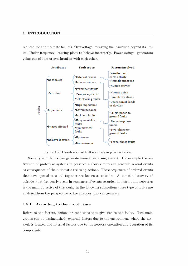
energising transformers) or components malfunction. Fig. 1.2 shows fault classification
based on the most common criteria. Nevertheless, in the literature other attributes,
groups and subgroups can be found. For example, in (IDC-Technologies, 2000) faults
are classified into two main areas: active and passive. The active fault is when fault cur-
rent flows from one phase conductor to another (phase-to-phase) or alternatively from
one phase conductor to earth (phase-to-earth). This type of fault can also be further
classified into two groups, namely the solid fault and the incipient fault. The solid fault
occurs as a result of an immediate complete breakdown of insulation as would happen
if, say, a pick struck an underground cable, bridging conductors etc. or the cable was
dug up by a bulldozer. In these circumstances the fault current would be very high,
resulting in an electrical explosion. Incipient faults are those that start from very small
beginnings, from say some partial discharge (excessive electronic activity often referred
to as Corona) in a void in the insulation, increasing and developing over an extended
period, until such time as it burns away adjacent insulation, eventually running away
and developing into a solid fault. Passive faults are conditions that are stressing the
system beyond its design capacity, so that ultimately active faults will occur. Typical
examples are: overloading –leading to overheating of insulation (deteriorating quality,
9
1. INTRODUCTION
reduced life and ultimate failure). Overvoltage –stressing the insulation beyond its lim-
its. Under frequency –causing plant to behave incorrectly. Power swings –generators
going out-of-step or synchronism with each other.
Figure 1.2: Classification of fault occurring in power networks.
Some type of faults can generate more than a single event. For example the ac-
tivation of protective systems in presence a short circuit can generate several events
as consequence of the automatic reclosing actions. These sequences of ordered events
that have special sense all together are known as episodes. Automatic discovery of
episodes that frequently occur in sequences of events recorded in distribution networks
is the main objective of this work. In the following subsections these type of faults are
analysed from the perspective of the episodes they can generate.
1.5.1 According to their root cause
Refers to the factors, actions or conditions that give rise to the faults. Two main
groups can be distinguished: external factors due to the environment where the net-
work is located and internal factors due to the network operation and operation of its
components.
10

1.5 Fault classification and episodes
1.5.1.1 Externals causes
These are all factors do not own the network, capable of causing faults. Environment
and weather are the main external causes of faults in power networks.
• Trees and animals: Animal contacts or tree contacts usually cause short circuits
especially in overhead lines. While animal contacts take place during daytime and
usually imply the apparition of events with significant arc voltage, tree contact
events take place at the end of the year (fall) and have low zero sequence voltage
values (Barrera, 2012).
• Weather and earth activities: Voltage events resulting from external causes
are highly influenced by weather conditions. It includes fault caused by agents
such as wind, snow, storms or lightning, but also others factors as landslides,
floods, fire or earthquakes. Lightning induced events occur mainly during night
as well as in the first two-thirds of the year (Barrera, 2012).
• Human activities: Excavations, vandalism and other activities of individuals
are also important causes of faults in power distribution networks.
1.5.1.2 Internals causes
Includes all factors related to the proper condition of the network or its components
that can cause faults.
• Component aging: These faults are caused by the degradation of materials
and/or components, that under certain environmental conditions produce partial
discharges (Zhang and Gockenbach, 2007). This type of fault evolves and develops
over an extended period of time (days or months), and the rate of occurrence
increases due to the acceleration of the degradation process (Kim et al., 2004;
Moghe and Mousavi, 2009). When these phenomena happen, the disturbances
generated are usually not detected by the protective systems, and specific devices
such as power quality monitors, must be installed to capture such events (Bowers
et al., 2008). Their evolution is expected to end as a permanent failure; so
the recognition and monitoring of these events can prevent the occurrence of
permanent faults.
11

1. INTRODUCTION
• Cumulative stress on electrical components: Failures in electrical compo-
nents may occur from electrical and mechanical stress (Zhang and Gockenbach,
2007). This stress may be originated during the occurrence of previous faults at
other points of the network or by an intensive use of the infrastructure during
long periods of time. In the first case, a sequence of events produced by subse-
quent faults in a feeder can be considered as a predictive episode that alerts of
possible failures in components located in the path between the transformer and
the location of previous faults associated with the events in the episode.
• Normal operation of important loads: Several events are caused by the oper-
ation of the equipment itself or significant loads connected to the network, mainly
when connecting and disconnecting manoeuvres are performed. The switching of
large loads can be viewed as voltage or current events. The regular occurrence
of similar events may be indicative of this type of situation and their appearance
probably follows patterns associated with the operation of those loads, so their
characterisation could be used as a filtering method to separate them from events
due to fault situations.
• Abnormal operation of devices or equipment on the network: Equipment
connected to the network inappropriately can cause intermittent variations in
current or voltage during short periods of time and even activate the protective
system. For example, the incorrect connection of capacitor banks can produce
transient overvoltage during the energising process that are reproduced every time
a new energising is done. The identification and characterisation of this events
would allow them to be filtered from the ones due to fault conditions.
1.5.2 According to their duration
The duration of faults is related with extent of damage on the network or its components
and the time required to restore normal conditions of power supply.
1.5.2.1 Permanent faults
These faults are usually associated with short circuits or a breakdown of insulation
between two or more conductors that cause the actuation of protective systems to
isolate, locate and restore the fault. Permanent fault are short circuits that will persist
12

1.5 Fault classification and episodes
until they are repaired by human intervention. As a consequence of these faults, several
voltage dips similar in shape and duration are generated at time intervals that depend
on the settings of protective systems, fault location and restoration strategies (Quiroga
et al., 2010b). Examples of permanent faults include insulators damaged by flashover,
underground cable breakdown and surge arrester damage.
1.5.2.2 Temporary faults
These are short circuits that will clear after the faulted component (typically an over-
head line) is de-energized and reenergized. In this category low impedance faults pro-
duced by the interaction of external agents with the network (lightning strikes, wind,
transient tree contacts, etc.) during a short period of time are included. They activate
protective systems, allowing the circuit to be re-energised (fault clearing) after a reclos-
ing operation. Although they are not associated with fault components of the power
system, they can affect their performance. Moreover, the events generated by this type
of fault are expected to be independent of each other.
1.5.2.3 Self-clearing faults
These are short circuits extinguished themselves without any external intervention.
This type of faults can occur for example in the degradation process of cables due to
insulation breakdown from water penetrating into splices (Stringer and Kojovic, 2001).
When water accumulates in a cable splice, it leads to an insulation breakdown followed
by an arc. Arcing causes rapid water evaporation and develops high pressures inside the
splice which extinguishes the arc and interrupts the current. Because the fault current
is interrupted by water vapor pressure developed from fault current, these types of
faults are called self-clearing. Their frequency of occurrence increases over time. At
first, they occur infrequently, once a month, then several times a week, then several
times a day, and finally several times an hour until the splice fails, damaging the cable.
1.5.3 According to their impedance
The magnitude of faults is usually related with the severity of the short circuit and the
current values during their occurrence. Bolted or solid faults cause more severe faults
than impedance faults.
13

1. INTRODUCTION
1.5.3.1 Low impedance faults
These are fault conditions in which the fault current magnitude is enough to be detected
by conventional overcurrent relays or fuses, so they activate the protective system of
the networks.
1.5.3.2 High impedance faults
These are fault conditions in which the fault current magnitude is not high enough
to be detected by conventional overcurrent relays or fuses, so they do not activate
any protection. A high impedance fault results when an energised primary conductor
comes in contact with a quasi-insulating object, for example a tree, a structure or
equipment, or falls to the ground. Often this leaves an energised conductor on the
ground posing a danger to the public as well as a risk of arcing ignition of fires. The
diagnosis of such faults is based on the detection of some abnormal features (harmonics,
arcing, etc.) that can be extracted from the current and/or voltage but requires the
installation of specific devices to be detected (Vico et al., 2010). They are associated
with unpredictable phenomena, so it is very difficult to forecast them and only detection
can be addressed.
1.5.3.3 Incipient faults
Misbehaviours in the power system typically associated with leakage current in elec-
trical components. They are an intermittent and transient phenomena that only take
place under specific conditions, usually related with symptoms of component failures.
Despite not producing energy variations capable of activating protections, they generate
disturbances of low magnitude that propagate across the network.
1.5.4 According to the number of affected phases
Given that distribution systems are three-phase systems, a fault can involve one or sev-
eral phases of the systems. Two main groups can be distinguished: symmetrical and
unsymmetrical faults. The fault impedance are related with the number of phases af-
fected by the fault. This attribute is useful to estimate the magnitude and the pinpoint
location of the fault.
14

1.5 Fault classification and episodes
1.5.4.1 Symmetrical faults
It refers to faults that affect simultaneously the three phases. Three-phase faults are
more severe than unsymmetrical faults, but the latter are much more frequent.
1.5.4.2 Unsymmetrical faults
It refers to faults where not all phases of the power system are involved.
• Single-phase-to-ground faults: These are the more frequent faults, they rep-
resent more than 80% of the total faults in the system.
• Phase-to-phase faults: Two phases of the system are involved but they are
isolated with respect to ground.
• Phase-to-phase-to-ground faults: A two-phase-to-ground fault is similar to
a phase-to-phase fault, but current flows from phase to ground during the fault.
In general, the distribution probability of faults is around 80%, 10%, 5% and 5% for
single-phase-to-ground, two-phase-to-ground, phase-to-phase and three-phase faults,
respectively (Olguin, 2005).
1.5.5 According to their relative location
It refers to the fault source relative location from a monitored point in the network.
Usually power quality monitors are installed at the bus bar of the distribution sub-
station. So, they can distinguish between fault occurred in distribution system or
downstream and transmission system or upstream.
1.5.6 Evolution of failures and faults
If we consider the analysis of a set of faults monitored in an individual point of the
distribution network such as feeder head, probable dependency relationships among
some of the fault situations described previously would be found. For example, an
insulator under successive overvoltages caused by faults in the network may fail due
to the accumulated stress, then successive transient o permanent faults may cause a
new fault by cumulative stress in other point of the network. Possible influences are
summarised in the schema of Fig. 1.3. Blocks are used to indicate faulty states, arrows
15

1. INTRODUCTION
causal dependencies among faulty states and circles represent the combination of effects.
Thus, arrows indicate possible transitions between faulty states.
Figure 1.3: Links between different fault situations.
According to Fig. 1.3, the operation of loads or devices in the network, can lead
to the emergence of permanent or transient faults, is the case for example of motor
starting, transformer energization, capacitor banks operation, etc. In turn, the effects
generated by these faults cause stress on other components such as switches, cables and
insulators. This stress is manifested in the form of incipient faults which subsequently
evolve into states of permanent faults. Likewise, the external factors influence the
emergence of permanent faults, transient faults, incipient faults or by cumulative stress.
Each of these types of faults can evolve to other states in the same or other network
components. In summary, due of the physical connection and interaction between the
different components of the power network, the condition of each component, is linked
–to a greater or lesser extent– to the state of other components.
Notice that the events generated by those faults can present different shapes depend-
ing on factors such as the phases affected, including the number of phases or imbalance,
the load (presence of laterals, affected load, etc.), fault impedance (high/low, resistive
or none), type of affected line (aerial, cable or combination of the both), etc. The study
of significant features for each type of fault and the episode associated with them offers
possible ways of automatically discriminating according to fault causes or using them
as prediction tools (Barrera et al., 2010).
16
1.6 Main contributions of this work
1.6 Main contributions of this work
This thesis manuscript reports the research work developed by the author about the
automatic discovery of meaningful patterns in sequences of events recorded in power
distribution systems. Chapter 1 contains a basic review of the approaches related to
treatment of events recorded in power distribution networks useful for power quality
monitoring and assessment. Likewise, this chapter contains aspects related with the
origin and nature of faults and other misbehaviours of the power distribution networks,
their classification and relationships between events due to faults.
This thesis proposes the use of sequence pattern discovery algorithms to find relevant
patterns in data bases of historical events recorded in power distribution networks. The
main contributions of the work are summarised as follows:
1. Representation of power quality events as attribute-value tuples and sequences
of them generated by faults and failures as episodes. Adaptation of pattern
sequence discovery problem to deal with sequences of power events and its general
formulation. This topics are presented in Chapters 1 and 2 of this thesis and they
were partially published in (Melendez et al., 2012).
2. A new algorithm for frequent episode discovery is proposed. A comprehensive
review of existing algorithms was made. The proposed algorithm avoids over-
count and missing of occurrences, which are common problems in other pattern
sequence discovery algorithms. Chapter 2 contains the proposed algorithm and
their main principles were published in (Quiroga et al., 2012a).
3. A strategy to guide the search of episodes related/unrelated with events prede-
fined by the user is proposed. This strategy allows the extraction of significant
episodes from the point of view of the priority events in the mining process. A
particular case is given when the analysis focuses on episodes containing specific
events, exploration of other unrelated episodes is avoided. This contribution is
presented in Chapter 3 and also was published in (Quiroga et al., 2012b).
4. Two new indexes for assessing the causality of frequent episodes are proposed.
They are suggested as complementary criteria to the confidence of the episode
rule. The first one, named cohesion of the episode, is based on the comparison
17

1. INTRODUCTION
of the number of serial and parallel occurrences, whereas the second, named
backward-confidence of the episode, is analogous to the confidence of an episode
rule but it focuses on the beginning of the episode instead of the end. The cited
indexes are presented in Chapter 3 and they were published in (Quiroga et al.,
2011b, 2012a).
5. Application of proposed methods (frequent episode discovery and significant episodes
recognition) with voltage dips and incident data bases to discover relevant pat-
terns. Episodes related with permanent and transient faults, as well as other
interesting patterns from causes point of view, are found using the algorithms.
The analysis of these data sets was part of the research projects ‘Monitorizacion
Inteligente de la Calidad de la Energıa Electrica’ (DPI2009-07891) and “EN-
ERGOS, CEN20091048: Tecnologıas para la gestion automatizada e inteligente
de las redes de distribucion energetica del futuro” (PROGRAMA CENIT-2009).
Chapters 4 and 5 are focused in the analysis of the cited data sets and results
have been also reported in (Melendez et al., 2012; Quiroga et al., 2010a, 2011b,
2012b, 2010b).
The manuscript is self contained and provides references that supported the contents
of this research.
1.7 List of publications
This thesis is partially based on the work reported in the following publications.
• Journals
1. O. Quiroga, J. Melendez, S. Herraiz. Pattern discovery in sequences of incidentscollected in power distribution systems, Engineering Applications of Artificial Intel-ligence.Submitted on July 31, 2012 .
2. J. Melendez, O. Quiroga, S. Herraiz, Analysis of sequences of events for the char-acterisation of faults in power systems, Electric Power Systems Research (EPSR),DOI: 10.1016/j.epsr.2012.01.010, vol. 87, pp. 22 - 30, 2012, (Melendez et al., 2012).
• Conferences
18

1.8 Outline of the thesis
1. O. Quiroga, J. Melendez and S. Herraiz, Frequent and significant episodes in se-quences of events: Computation of a new frequency measure based on individualoccurrences of the events, 4th International Conference on Knowledge Discoveryand Information Retrieval KDIR 2012. Barcelona, Spain, 4-7 Oct. 2012, (Quirogaet al., 2012a).
2. O. Quiroga, J. Melendez, S. Herraiz, A. Ferreira, A. Munoz. Analysis of frequentepisodes in sequences of incidents collected in power distribution systems, 2nd. IEEEPES European Conference and Exhibition on Innovative Smart Grid Technologies(ISGT-EUROPE 2011). Manchester, UK, 5-7 Dec. 2011, (Quiroga et al., 2011b).
3. O. Quiroga, J. Melendez, S. Herraiz. Fault Causes Analysis in Feeders of PowerDistribution Networks, International Conference in Renewables Energies and Qual-ity Power ICREP’11. Las Palmas de Gran Canaria, Spain, 13 -15 Apr. 2011,(Quiroga et al., 2011a).
4. O. Quiroga, J. Melendez and S. Herraiz. Fault-Pattern Discovery in Sequencesof Voltage Sag Events, in 14th IEEE International Conference on Harmonics andQuality of Power (ICHQP), Bergamo, Italy., 26-29 Sept. 2010, (Quiroga et al.,2010a).
5. O. Quiroga, J. Melendez and S. Herraiz. Sequence Pattern Discovery of EventsCaused by Ground Fault Trips in Power Distribution Systems, 18th MediterraneanConference on Control and Automation, MED’10. Marrakech, Morocco, June 23-25, 2010, (Quiroga et al., 2010b).
6. O. Quiroga, J. Melendez, S. Herraiz, J. Sanchez. Analysis of Event sequences inPower Distribution Systems, International Conference in Renewables Energies andQuality Power ICREP’10. Granada, Spain, 23 - 25 Mar. 2010, (Quiroga et al.,2010c).
1.8 Outline of the thesis
The thesis is organised in six chapters. Chapter 1 introduces the general background
of the work, motivation and objectives. The rest of the thesis document is organised
as follows.
• Chapter 2 – Mining sequences of events: This chapter presents the prin-
ciples used for frequent pattern discovery in sequences of events. The main pro-
cedure used in the search for episodes and several algorithms to compute their
frequency are described. A new algorithm to improve results of the mining process
is proposed and validated using synthetic data sets.
19

1. INTRODUCTION
• Chapter 3 – Significant episodes in sequences of events: This chapter
presents different approaches for recognising significant events and meaningful
patterns once the discovery algorithms have identified frequent patterns. Methods
used to assess the quality of episodes are described and two new indexes for
assessing the causality and the strength of the order relation expressed by frequent
episodes are proposed and tested using synthetic data sets.
• Chapter 4 – Mining voltage dip sequences recorded in power distribu-
tion substations: This chapter adopts strategies proposed in previous chapters
for discovering significant frequent patterns from data bases of events collected
by power quality monitors installed in the secondary of distribution substations
in a real network. A dataset of voltage dip events recorded in a power distribu-
tion network is analysed and different types of associations between events are
discovered and their physical meaning is discussed.
• Chapter 5 – Pattern discovery in sequences of incidents collected in
power distribution networks: This chapter presents the analysis of a dataset
of incidents –faults or situations that affect the continuity of supply – collected in
a power distribution network. Order relations between main causes of incidents
on the network are discovered and their physical meaning is discussed.
• Chapter 6 – Conclusions and future work: Main conclusions and contri-
butions of this thesis are emphasized in this chapter. Some research issues are
identified and proposed for future work.
Finally, references and an appendix are included. The appendix presents a method
for identification of transient faults events in sequences of voltage dips from their sim-
ilarities in magnitude and duration, results are presented and discussed.
20

2
Mining sequences of events
This chapter presents the frequent pattern discovery fundamentals used for mining
event sequences. General background, formal definitions and related concepts and pro-
cedures for mining sequences of events are introduced in the chapter. The majority of
these algorithms are based on proposing candidates and finding the most frequent, in
terms of number of counted occurrences, in a given sequence following an iterative pro-
cedure. Different methods proposed in the literature for the computation of frequency
of episodes are presented and discussed. Besides, a new algorithm to extract frequent
episodes is proposed. Improvements of this new method are includes the ability to deal
with serial and parallel episodes and allowing different restrictions among events in the
episode. Performance of the method is evaluated with synthetic data to quantify the
benefits.
2.1 Introduction
Given the advances in monitoring systems and data storage, a new approach has become
important for the prediction of failures in complex systems. This new approach includes
the analysis of large blocks of information, which is known as data mining.
Data mining is the process of automatic or semiautomatic exploration and analysis
of large amounts of stored data to discover useful structures hidden in the data such
as regularities or correlations. In general, models or patterns are the two types of
structures that can be found by data mining algorithms.
21

2. MINING SEQUENCES OF EVENTS
A model can be defined as a global summary of the data, which is often obtained in
the form of some functional relationship among the variables (or attributes) in the data.
The idea here is to understand the underlying data generation process. In contrast to
a model, a pattern is a local structure or regularity in the data. The role of patterns
in data mining would be to bring to the attention of some interesting structures in
the data rather than provide summary information about the whole data generation
process (Murthy, 2007).
Multivariate statistical techniques are widely used to model multi attributes data
sets. These techniques can be classified into two main groups depending on the nature
of the monitored variables: dependence methods and interdependence methods. De-
pendence methods are applied when the variables in the dataset are divided into two
groups: dependent and independent. The objective is to discover the relationships be-
tween the sets of independent and dependent variables. This group includes techniques
such as multi linear regression (MLR), multivariate analysis of variance (MANOVA),
discriminant analysis (DA). Interdependence methods are applied when dependent and
independent set of variables are not distinguished in the data set. The aim is to identify
which variables are linked together and interpret how this relationship is established.
Techniques such as principal component analysis (PCA), Cluster analysis (CA) or fac-
tor analysis (FA) are part of this group. Following this paradigm, other methods and
algorithms coming from the Artificial Intelligence community have been proposed for
learning such relationships using data sets. Examples of them are the artificial neural
networks, Bayesian networks, decision trees, support vector machines and so on.
Patterns is the type of structures searched in many application domains such as clin-
ical monitoring, alarm management systems, customer transactions, query databases.
When this data has a time dimension or sequential order then they must be treated
differently in order to recognize the existence of such temporary or causal structures.
This research field is known as sequential data mining and/or temporal data mining
(Roddick and Spiliopoulou, 2002). Depending on the nature of the data, there are two
main approaches to automatically discover patterns in sequences using different order
criteria between the elements of the sequence: sequential pattern mining (Agrawal and
Srikant, 1995) and frequent episode discovery (Mannila et al., 1997). Both approaches
are oriented to the analysis of sets of discrete events with time dependencies (Laxman
and Sastry, 2006). The fundamentals of each one are described below.
22
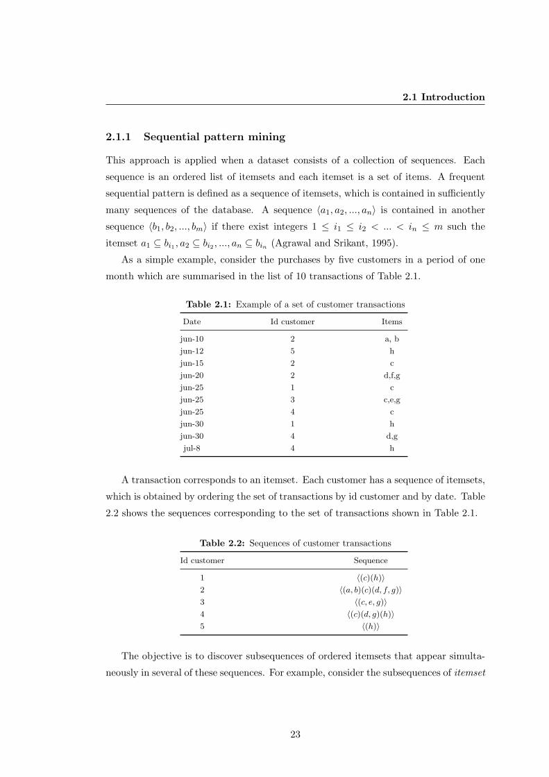
2.1 Introduction
2.1.1 Sequential pattern mining
This approach is applied when a dataset consists of a collection of sequences. Each
sequence is an ordered list of itemsets and each itemset is a set of items. A frequent
sequential pattern is defined as a sequence of itemsets, which is contained in sufficiently
many sequences of the database. A sequence 〈a1, a2, ..., an〉 is contained in another
sequence 〈b1, b2, ..., bm〉 if there exist integers 1 ≤ i1 ≤ i2 < ... < in ≤ m such the
itemset a1 ⊆ bi1 , a2 ⊆ bi2 , ..., an ⊆ bin (Agrawal and Srikant, 1995).
As a simple example, consider the purchases by five customers in a period of one
month which are summarised in the list of 10 transactions of Table 2.1.
Table 2.1: Example of a set of customer transactions
Date Id customer Items
jun-10 2 a, b
jun-12 5 h
jun-15 2 c
jun-20 2 d,f,g
jun-25 1 c
jun-25 3 c,e,g
jun-25 4 c
jun-30 1 h
jun-30 4 d,g
jul-8 4 h
A transaction corresponds to an itemset. Each customer has a sequence of itemsets,
which is obtained by ordering the set of transactions by id customer and by date. Table
2.2 shows the sequences corresponding to the set of transactions shown in Table 2.1.
Table 2.2: Sequences of customer transactions
Id customer Sequence
1 〈(c)(h)〉2 〈(a, b)(c)(d, f, g)〉3 〈(c, e, g)〉4 〈(c)(d, g)(h)〉5 〈(h)〉
The objective is to discover subsequences of ordered itemsets that appear simulta-
neously in several of these sequences. For example, consider the subsequences of itemset
23

2. MINING SEQUENCES OF EVENTS
that appear in at least two sequences in Table 2.2, then the results are: 〈(c)(h)〉 and
〈(c)(d, g)〉. They constitute the sequential patterns of this dataset.
Several algorithms such as SPADE (Zaki, 2001), PrefixSpan (Prefix-projected Se-
quential pattern mining) (Pei et al., 2001), SaM (Split and Merge Algorithm) (Borgelt,
2010), Relim (Recursive Elimination Algorithm) (Borgelt, 2005), LCM (Linear Closet
Item set Miner) (Uno et al., 2004), have been developed for the discovery of sequential
patterns. This is an issue in continuous development that is part of the frequent item-
set mining in transaction databases, research field that covered other topics such as
structured pattern mining, correlation mining, associative classification, and frequent
pattern-based clustering, as well as their broad applications (Han et al., 2007).
2.1.2 Frequent episode discovery
The starting point are data sets organised as a single long sequence of events where
each event is described by its type and its time of occurrence.
Definition 2.1. Event. An event is defined by the pair (e,t) where t denotes theoccurrence time (time stamp) and e represent the event attributes (one or several) thatcontain the information useful to characterise the event. Event attributes can be asingle label or a vector of continuous/discrete attribute-value pairs defined in a givenrange or set of predefined values (Mannila et al., 1997).
Definition 2.2. Sequence of events. A sequence of events S is an ordered listof events or a n-tuple S = 〈(e1, t1), (e2, t2), ..., (en, tn)〉 where ti ≤ ti+1 for all i ∈{1, 2, ..., n− 1}. The length of S, |S|, is n. In single sequence mining, the events arerepresented categorically from a finite set A of event types where ei ∈ A (Mannila et al.,1997).
The following is an example of a sequence of events.
S1 = 〈(a, 5), (d, 10), (a, 20), (b, 25), (c, 30), (b, 36), (a, 40), (d, 51), (a, 55), (b, 60), (c, 68)〉(2.1)
In this example, the length of the sequence is 11, and A is a set of 4 different types
of events, A = {a, b, c, d}. The sequence can be represented graphically as shown in Fig
2.1. In the basic framework, the events are essentially instantaneous; this means that
events occur at a given instant and have not a duration associated.
24

2.1 Introduction
Figure 2.1: Graphic representation of an event sequence.
The mining objective is to find collections of partially ordered events occurring
together within the sequence. This collection of events are called episodes.
Definition 2.3. Episode. An episode α is an ordered list formed by event types inA (set of event types) of the form α = 〈a1, a2, ..., am〉 with aj ∈ A for all j = 1, ...,m.The size of α is the number of elements in α that is |α| = m.
For example, in the sequence of Fig. 2.1 the events a, b and c can conform
and episode, α = 〈a, b, c〉, which have at least two occurrences along the sequences:
〈(a, 20), (b, 25), (c, 30)〉 and 〈(a, 55), (b, 60), (c, 68)〉. The frequency or support of an
episode is equal to its number of occurrences and a minimum frequency threshold must
be specified to consider an episode as frequent.
Definition 2.4. Occurrence of an episode. An episode α = 〈a1, a2, ..., am〉 occursin a sequence of events S = 〈(e1, t1), (e2, t2), ..., (en, tn)〉 if there is at least one orderedsequence of events S′ = 〈(ei1 , ti1), (ei2 , ti2), ..., (eim , tim)〉 such that S′ ⊆ S and aj = eijfor all j = 1, 2, ...,m. Usually an occurrence is denoted as o = 〈i1, i2, ..., im〉 whereo [j] = ij and j = 1, 2, ...,m.
Definition 2.5. Frequency or support of an episode. It is the number of oc-currences of an episode over a sequence of events. The frequency of an episode α isabbreviated as fr(α).
Definition 2.6. Frequent episode. An episode α is frequent if its number of oc-currences fr(α) is equal or greater than a threshold (min fr), i.e., α is frequent iffr(α) ≥ min fr.
25

2. MINING SEQUENCES OF EVENTS
2.2 Analysis of sequences of events registered in power
distribution systems
The previous definitions have been adapted to deal with disturbances, i.e. power or
electrical events, collected by power quality monitors installed in substations and/or
consumers. A set of timestamped events recorded at a single point of the network
during a power quality monitoring campaign is considered as a sequence of events.
Definition 2.7. Electrical event. An electrical event, ei(ti), is a dated record ofan electric variable, typically currents and voltages, that suffers a sudden variation inits value. It is defined by an (m+1)-tuple, (a1, . . . , am, ti), where ti is the event timestamp (usually, the starting time) and aj (with j = 1, . . . ,m) represents the value ofeach attribute, Aj , defined in its respective domain, aj ∈ Dom(Aj). Event attributescan be continuous (duration, magnitude, maximum peak, frequency content, etc.) orsymbolic (type of incident, causes, affected phases, etc.). The attributes are selectedaccording to their relevance with respect to the proposed goal.
A sequence of events can contain several events, but only some subsets of them
are of interest, either because they present similar features (shape, duration, etc.) or
because there is some relationship that allows them to be considered together (timing,
periodicity, etc.), as for example, when they are originated by the same cause in an
evolving fault. According to the nomenclature introduced in Section 2.1.2, these subsets
of significant events in a sequence are called episodes and are expected to describe some
patterns. The existence of those patterns is exploited, taking advantage of mining
algorithms to automatically obtain those patterns from an existing sequence of events
based on the criterion of frequent episodes. Once those patterns are known, they can
be used to better describe fault situations and their evolution. They can also be used
to predict future failures by recognising the events that match the early stages of a
pattern.
In the remainder of this chapter, common terminology, fundamentals and main
methods used in single sequence mining are presented. Likewise, a new algorithm to
improve results of the mining process is proposed.
26

2.3 Background on event sequences mining
2.3 Background on event sequences mining
Frequent episodes mining in sequences of events has been applied in many application
domains: analysing alarm sequences in telecommunication networks (Mannila et al.,
1997), web access pattern discovery and family protein analysis (Casas-Garriga, 2003),
fault prognosis based on logs of manufacturing plants (Laxman et al., 2007), study of
multi-neuronal spike train recordings (Patnaik, 2006) or event tracking problems for
news stories (Iwanuma et al., 2005).
Typically, methods for mining frequent episodes in a sequence follow an iterative
procedure that starts searching for frequent events (single event episodes). The can-
didate episodes are generated by aggregating frequent events. Occurrence of these
candidate episodes is evaluated to check if their frequency is over a minimum threshold
to be considered a frequent pattern. This basic procedure shown in Algorithm 1, is
based on the same general idea as the Apriori algorithm (Agrawal and Srikant, 1995).
Algorithm 1 General method for frequent episode discoveryInput: A sequence of events S, the set of event types or categories (E), and the minimum frequency
threshold min fr.
Output: Frequent episodes of length L, FL.
Procedure:
1: Initialise a counter associated with the length of episodes (L = 1).
2: Generate the first set of candidate episodes CL (L = 1) from the frequent events in E.
3: while CL 6= {} do
4: Compute the frequency (fr) of the candidate episodes of length L.
5: Extract and store frequent episodes (fr ≥ min fr) as FL.
6: Increase the counter in 1: L← L+ 1.
7: Generate candidate episodes of length L, CL, from the frequent episodes in FL−1.
The first set of candidate episodes C1 (length L = 1) is generated by using the set
of event types E that appears in the sequence (line 2). In the main function (line 4),
the number of occurrences fr of each candidate episode is computed and those with fr
over the threshold are classified as frequent episodes and stored as FL (line 5). From
frequent episodes in FL, a new set of candidate episodes, CL, of length L = L + 1,
is build (line 7). The process continues iteratively until no candidate episodes are
found (CL = {}) (line 3). In the literature, frequent episode discovery algorithms differ
mainly in the way of searching and computing the frequency of the candidate episodes
(line 4).
27
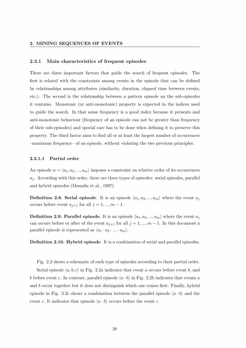
2. MINING SEQUENCES OF EVENTS
2.3.1 Main characteristics of frequent episodes
There are three important factors that guide the search of frequent episodes. The
first is related with the constraints among events in the episode that can be defined
by relationships among attributes (similarity, duration, elapsed time between events,
etc.). The second is the relationship between a pattern episode an the sub-episodes
it contains. Monotonic (or anti-monotonic) property is expected in the indices used
to guide the search. In that sense frequency is a good index because it presents and
anti-monotonic behaviour (frequency of an episode can not be greater than frequency
of their sub-episodes) and special care has to be done when defining it to preserve this
property. The third factor aims to find all or at least the largest number of occurrences
–maximum frequency– of an episode, without violating the two previous principles.
2.3.1.1 Partial order
An episode α = 〈a1, a2, ..., am〉 imposes a constraint on relative order of its occurrences
aj . According with this order, there are three types of episodes: serial episodes, parallel
and hybrid episodes (Mannila et al., 1997).
Definition 2.8. Serial episode. It is an episode 〈a1, a2, ..., am〉 where the event aj
occurs before event aj+1 for all j = 1, ...,m− 1.
Definition 2.9. Parallel episode. It is an episode 〈a1, a2, ..., am〉 where the event aj
can occurs before or after of the event aj+1 for all j = 1, ...,m− 1. In this document aparallel episode is represented as 〈a1 · a2 · ... · am〉.
Definition 2.10. Hybrid episode. It is a combination of serial and parallel episodes.
Fig. 2.2 shows a schematic of each type of episodes according to their partial order.
Serial episode 〈a, b, c〉 in Fig. 2.2a indicates that event a occurs before event b, and
b before event c. In contrast, parallel episode 〈a · b〉 in Fig. 2.2b indicates that events a
and b occur together but it does not distinguish which one comes first. Finally, hybrid
episode in Fig. 2.2c shows a combination between the parallel episode 〈a · b〉 and the
event c. It indicates that episode 〈a · b〉 occurs before the event c.
28
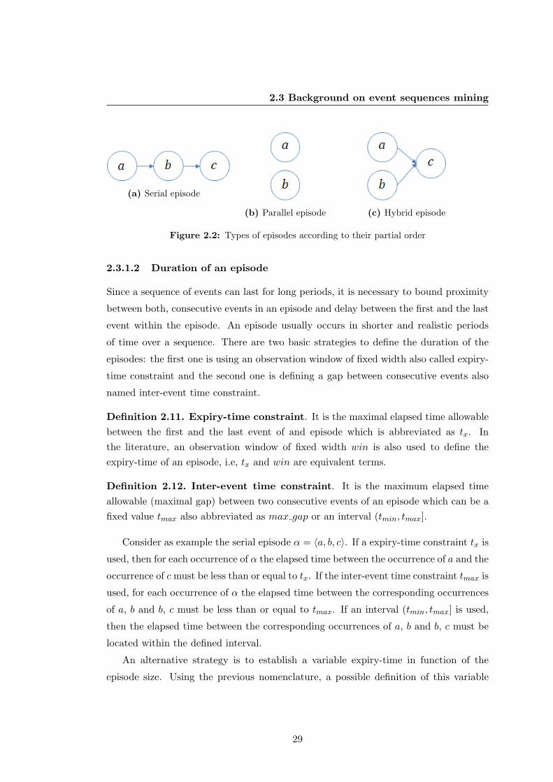
2.3 Background on event sequences mining
(a) Serial episode
(b) Parallel episode (c) Hybrid episode
Figure 2.2: Types of episodes according to their partial order
2.3.1.2 Duration of an episode
Since a sequence of events can last for long periods, it is necessary to bound proximity
between both, consecutive events in an episode and delay between the first and the last
event within the episode. An episode usually occurs in shorter and realistic periods
of time over a sequence. There are two basic strategies to define the duration of the
episodes: the first one is using an observation window of fixed width also called expiry-
time constraint and the second one is defining a gap between consecutive events also
named inter-event time constraint.
Definition 2.11. Expiry-time constraint. It is the maximal elapsed time allowablebetween the first and the last event of and episode which is abbreviated as tx. Inthe literature, an observation window of fixed width win is also used to define theexpiry-time of an episode, i.e, tx and win are equivalent terms.
Definition 2.12. Inter-event time constraint. It is the maximum elapsed timeallowable (maximal gap) between two consecutive events of an episode which can be afixed value tmax also abbreviated as max gap or an interval (tmin, tmax].
Consider as example the serial episode α = 〈a, b, c〉. If a expiry-time constraint tx is
used, then for each occurrence of α the elapsed time between the occurrence of a and the
occurrence of c must be less than or equal to tx. If the inter-event time constraint tmax is
used, for each occurrence of α the elapsed time between the corresponding occurrences
of a, b and b, c must be less than or equal to tmax. If an interval (tmin, tmax] is used,
then the elapsed time between the corresponding occurrences of a, b and b, c must be
located within the defined interval.
An alternative strategy is to establish a variable expiry-time in function of the
episode size. Using the previous nomenclature, a possible definition of this variable
29

2. MINING SEQUENCES OF EVENTS
expiry-time tx of an episode α can be tx = (|α| − 1) × tmax. In this case, for episodes
of size greater than two, the elapsed time between successive events is not constrained
(Casas-Garriga, 2003).
2.3.1.3 Derivations or extensions of an episode
Sub-episodes and super-episodes are the most common derivations and extensions of
an episode, respectively.
Definition 2.13. Sub-episode, super episode. An episode β = 〈b1, b2, ..., bm〉 is asub-episode of another episode α = 〈a1, a2, ..., an〉 if m < n and there exist 1 ≤ i1 <
i2 < ... < im ≤ n such that bj = aij for all j = 1, 2, . . . ,m. In this case, α is a superepisode of β.
In turn, the episode α in Definition 2.13 can be classified within three types of
super episodes of β, depending of the location of β within α: forward-extension super
episode, backward-extension super episode and middle-extension super episode (Zhou
et al., 2010).
Definition 2.14. Forward-extension super episode. The episode α in Defini-tion 2.13 is called the forward-extension super episode of β if there exist i1 = 1, i2 =2, · · · , im = m.
Definition 2.15. Backward-extension super episode. The episode α in Definition2.13 is called the backward-extension super episode of β if there exist i1 = n−m+1, i2 =n−m+ 2, · · · , im = n.
Definition 2.16. Middle-extension super episode. The episode α in Definition2.13 is called the middle-extension super episode of β if α is neither a forward-extensionnor backward-extension super episode of β.
2.3.1.4 Parts of an episode
The parts of an episode are related with the relative location of the event within it.
Suffix and prefix are the most important parts.
Definition 2.17. Suffix of an episode. The suffix of an episode α is defined as thelast event in the episode and it is abbreviated suffix(α), i.e., if α = 〈a1, a2, ..., am〉,then suffix(α) = 〈am〉,
30

2.3 Background on event sequences mining
Definition 2.18. Prefix of an episode. The prefix of α is the episode composedby all elements in α without the last one. It is abbreviated as prefix(α). I.e., ifα = 〈a1, a2, ..., am〉, then prefix(α) = 〈a1, a2, ..., am−1〉.
Definition 2.19. Large suffix of an episode. The large suffix of an episode is definedin this work as the episode composed by the elements in α without the first one and itis abbreviates as lsuffix(α). If α = 〈a1, a2, ..., am〉, then lsuffix(α) = 〈a2, ..., am〉.
2.3.1.5 Types of occurrences
After defining the limits of duration of episodes (Definitions 2.11 or 2.12), the oc-
currences of an episode refer to parts of the sequence containing the episode. Such
occurrences can be normal occurrences as shown in Definition 2.4 or minimal occur-
rences.
Definition 2.20. Minimal occurrence. An occurrence of α, o = 〈i1, i2, ..., im〉, isminimal if no other occurrence o′ = 〈i′1, i′2, ..., i′m〉 exists in a sequence of events S,between the intervals [i1, im) or (i1, im] with [i′1, i
′m] ⊂ [i1, im]. A minimal occurrence
of an episode α is denoted as mo(α).
In turn, a set of occurrences, or minimal occurrences, of an episode can be classified
as redundant or non-redundant, if different occurrences have or do not have elements
in common, respectively.
Definition 2.21. Redundant occurrences, non-redundant occurrences. A setof occurrences of an episode α is called non-redundant if for any two occurrences o =〈i1, i2, ..., im〉 and o′ = 〈i′1, i′2, ..., i′m〉 no event occurs simultaneously in both, i. e.,eij 6= ei′j for all j ∈ {1, 2, ...,m}. Otherwise, this set of occurrences is redundant.
Likewise, a set of occurrences can be overlapped or non-overlapped depending of
the location of these occurrences over a sequence.
Definition 2.22. Overlapped occurrences, non-overlapped occurrences. Twooccurrences of an episode α in a sequence of events S, o = 〈i1, i2, ..., im〉 and o′ =〈i′1, i′2, ..., i′m〉, are non-overlapped if o[1] > o′[m] or o′[1] > o[m], where m = |α|.Otherwise, these two occurrences are overlapped.
31

2. MINING SEQUENCES OF EVENTS
2.3.1.6 Anti-monotonicity property
Anti-monotonicity property is a common principle that frequency measure methods
should obey in frequent pattern mining.
Definition 2.23. Anti-monotonicity of an episode. An episode is anti-monotonicif its frequency is no greater than the frequency of its sub-episodes i.e., any two episodesα and β, α ⊇ β follow the principle of anti-monotonicity if fr(α) ≤ fr(β).
The anti-monotonicity property guarantees that a candidate episode can be pruned
safely if any of its sub-episodes is infrequent, and any infrequent episode need to be
extended. However, when the strategy of inter-event time constraint (Definition 2.12)
is used for the duration of the episodes, the anti-monotonicity property of an episode
can not be applied based on the frequency of all its sub-episodes. Only the frequency
of its non-overlapped sub-episodes must be considered (Casas-Garriga, 2003). For ex-
ample, given the serial episode 〈a, b, c〉, and its sub-episode 〈a, c〉. The two episodes are
extracted using a maximal gap between events tmax. While in 〈a, b, c〉, events a and c
can be separated for 2× tmax time units, in its sub-episode 〈a, c〉 the events have only
a maximum gap of tmax time units. Since the gap between events is different in both
episodes, the sub-episode 〈a, c〉 may be less frequent than the episode 〈a, b, c〉.
2.3.1.7 Maximum frequency of an episode
Maximum frequency refers to the fact of finding all the occurrences of an episode under
a strategy of duration constraint and an anti-monotonic measure.
Definition 2.24. Maximum frequency. Given a sequence of events S, a strategyof duration constraint (Section 2.3.1.2) and an anti-monotonic measure, then the fre-quency (Definition 2.5) fr ∀ α and ∀ S, ¬∃ fr∗ such that fr∗(α) > fr(α). Itensures that no proper occurrences are missed in the computation of the frequency ofand episode (Gan and Dai, 2010).
2.3.2 Frequency measure methods
How occurrences of a candidate episode α are counted varies among the different al-
gorithms. Results depend on the duration constraint (Section 2.3.1.2) used to obtain
the episodes and the occurrences selected (Section 2.3.1.5). Beyond the duration, dif-
ferent methods have been proposed to cope with particularities of the occurrences of
32

2.3 Background on event sequences mining
an episode. The occurrences within an observation window (Definition 2.11), to count
only the minimal occurrences (Definition 2.20), to consider only non-overlapped occur-
rences (Definition 2.22), etc., are strategies implemented to select the most properly
occurrences of an episode. According to the types of occurrences selected, there are
two main groups of methods to compute the frequency of an episode: methods based
on occurrences and methods based on minimal occurrences. Next, a short description
of the most common algorithms is presented.
2.3.2.1 Methods based on occurrences
The most used strategy to compute the frequency of an episode consists in counting
the number of occurrences. However, once the duration of a candidate episode α has
been defined, there are different ways to count the associated occurrences:
• Fixed-width window frequency measure: This method, exposed in (Mannila
et al., 1997), uses a sliding window w of fixed width tx predefined by the user.
The original sequence S is transformed in a set of overlapped fixed-width windows
and the fraction of windows that contain the episode corresponds to its frequency.
fr(α,S, tx) =|{w ∈W (S, tx) such that α occurs in w}|
|W (S, tx)|(2.2)
where W (S, tx) is the set of all windows w on S.
With this method some occurrences of the episodes could be over-counted because
several windows could contain the same occurrence. The method is limited to
discover episodes with duration no greater than the window width.
• Total frequency measure: This method, described in (Iwanuma et al., 2005),
also uses a sliding window of fixed width to search the episodes, but only windows
headed by the first event of the candidate episode are taken into account for the
frequency measure. This constraint aims to avoid over-counting occurrences of
episodes. The anti-monotonic property is assured by defining the frequency of an
episode as the lower frequency of its sub-episodes.
This method can be summarised as follows: given a sequence of events S =
〈(e1, t1) , (e2, t2) , ..., (en, tn)〉 and the length of the window win, the frequency of
33

2. MINING SEQUENCES OF EVENTS
each candidate episode α = 〈a1, ..., am〉 is evaluated in two steps. First, the Head
frequency (H–freq) is computed as:
H-freq(S, α, win) =n∑
i=1
δ(S(ti, tj)), α) (2.3)
where S(ti, tj) = 〈(ei, ti), ..., (ej , tj)〉 and tj−ti ≤ win. The function δ of Equation
2.3 is defined as:
δ(〈(ei, ti), ..., (ej , tj)〉 , 〈a1, ..., am〉) ={1 if a1 ⊆ ei and 〈a2, ..., am〉 ⊆ 〈ei+1, ..., ej〉,0 otherwise.
(2.4)
The measure H–freq(S, α, win) counts the number of occurrences for the first
element a1 of α in S, whereas, for the second and later elements a2, ..., am,
H–freq(S, α, win) just checks whether each of a2, ..., am occurs in S or not. Then,
frequency of α may be greater than the frequency of some of its sub-episodes.
To ensure the anti-monotonicity of an episode, the Total frequency (T–freq) is
calculated in the next step considering also the Head frequency of their corre-
sponding sub-episodes, as:
T–freq(S, α, win) = min {H–freq(S, β, win)} (2.5)
where β ⊆ α.
The algorithm in (Iwanuma et al., 2005) was formulated only for serial episodes.
We propose an adaptation for this method, to count parallel occurrences.
Given a sequence of events S = 〈(e1, t1), (e2, t2), ..., (en, tn)〉 and the length of
the window win, the Head parallel frequency (H-pfreq) of each candidate episode
α = 〈a1 · ... · am〉 can be evaluated as:
H-pfreq(S, α, win) =n∑
i=1
δp(S(ti, tj)), α) (2.6)
where S(ti, tj) = 〈(ei, ti), ..., (ej , tj)〉 and tj − ti ≤ win. The function δp of Equa-
tion 2.6 is defined as:
34

2.3 Background on event sequences mining
δp(〈(ei, ti), ..., (ej , tj)〉 , 〈a1 · ... · am〉) ={1 if ei ⊆ 〈a1 · ... · am〉 and 〈a1 · ... · am〉 ⊆ 〈ei, ..., ej〉,0 otherwise.
(2.7)
Finally, the total parallel frequency measure (T-pfreq) is obtained from the head
parallel frequency as:
T-pfreq(S, α, win) = min {H-pfreq(S, β, win)} (2.8)
where β ⊆ α.
Redefining the function δp in Equation 2.7, the adaptation of the method to count
parallel occurrences is performed. Equations 2.6 and 2.8 are similar to Equations
2.3 and 2.5, respectively.
• Bounded list of occurrences: This algorithm, proposed by Huang and Chang
(Huang and Chang, 2008), also uses a sliding window of fixed-width. They define
the support of an episode as the number of windows that start with the first
element of the episode. When windows are overlapped this support can be anti-
monotonic, then they define an episode as frequent if and only if the supports of
the episode and its sub-episodes are at least greater than threshold specified by
the user.
• Variable-width window: In this method, exposed in (Casas-Garriga, 2003),
the search of an occurrence is constrained to a maximal gap (max gap) between
consecutive events in the episode. This maximal gap is a parameters specified
by the user. Then, the frequency is calculated following the same procedure
introduced for the fixed-width window method but in this case the width of
the window is updated according to the length of the candidate episode |α| as:
win = (|α| − 1)×max gap. The frequency of α in S is defined as:
fr(α,S,max gap) =|{w such that w ∈W (S,win) ∧ α occurs in w}|
|W (S, win)|(2.9)
whereW (S, win) is the set of all windows w in S with width win and |W (S, win)| =|S| − 1 + win− 1.
35

2. MINING SEQUENCES OF EVENTS
• Frequency based on maximal non-redundant sets of occurrences: This
method uses as constraint the maximal gap between events (Gan and Dai, 2010).
The occurrences of a candidate episode are constructed recursively appending to
the occurrence of its prefix the leftmost occurrence of its suffix considering the
maximal gap constraint.
2.3.2.2 Methods based on minimal occurrences
The other methodology used to compute the frequency of an episode is by its minimal
occurrences. Each minimal occurrence must follow the duration constraint. There are
several ways to group these minimal occurrences:
• Minimal occurrences within a fixed window width: This method, also
introduced by Mannila et al. (Mannila et al., 1997), considers only the minimal
occurrences of an episode. Given an episode α and an event sequence S, they
say that the interval [ts, te) is a minimal occurrence of α in S, if α occurs in
the window w = (w, ts, te), and if α does not occur in any proper subwindow
on w. For each frequent episode, information about the location of its minimal
occurrences is stored, then the locations of minimal occurrences of a candidate
episode α, are computed as a temporal join of the minimal occurrences of two
sub-episodes of α. The first sub-episode is the prefix of α, prefix(α) and the
second one is the large suffix of α, lsuffix(α). This method avoids counting
non-minimal occurrences.
• Minimal occurrences with maximal gap: This method forces two constraints
during the search (Meger and Rigotti, 2004): a maximal window width and a
maximal gap between events. The frequency of an episode is calculated as the
sum of all minimum occurrences between a variant window width whose value
increase between one and the maximal window width. With this method non-
minimal occurrences are not counted and the bound of window restricts the width
of occurrences.
• Non-overlapped frequency measure: This method defines the frequency of
an episode as the maximal cardinality of the sets of the non-overlapped occur-
rences (Laxman et al., 2007). Non-overlapped occurrences means that an occur-
rence must be finished before starting a new one (Definition 2.22).
36

2.3 Background on event sequences mining
2.3.3 Discussion about the frequency measure methods
Frequency measure methods aims to find all the occurrences of candidate episodes.
However, the episodes extracted for all of them have dissimilar characteristics in dura-
tion and in the number of occurrences extracted. Some occurrences can be over-counted
or omitted under the described methods. Given a candidate episode and a duration
constraint, to find its maximal number of non-redundant occurrences implies to con-
sider not only its minimal occurrences but also, their overlapped and non-minimal
occurrences.
Methods based on minimal occurrences are useful to plot the occurrences of an
episode. They locate each occurrence in the process of computing frequency. Methods
that use observation windows only show the index of the windows where are located the
occurrences. Some methods find the occurrences of the episodes from the sub-episodes
locations (indexes). Such algorithms are faster, but can propagate errors due to the
improper selection of the sub-episode occurrences. Consequently, proper occurrences
of an episode would be ignored (missed).
Table 2.3 summarise the main characteristics of the methods described in Section
2.3.2. A list of five features for the episodes is shown. Partial order is abbreviated as (S)
or (P) for serial and parallel episodes, respectively. Duration is abbreviated as (1), (2)
or (3) for expiry-time constraint, inter-event time constraint or combination of both,
respectively. Likewise, four aspects about the occurrences is indicated: (R) over-count
occurrences , (M) missed or omit occurrences, (L) index or locate the occurrences and
(B) if the algorithm use the indexes of sub-episodes.
According with Table 2.3, methods of total frequency measure, maximal non-
redundant set of occurrences, minimal occurrences within a fixed-width window and
minimal occurrences with a maximal gap, are not defined for parallel occurrences.
However, for the total frequency measure method an adaptation to count parallel oc-
currences is proposed in Section 2.3.2.1 of this thesis.
Likewise, all review methods (except the method of non-overlapped occurrences)
are defined for episodes with expiry-time constraint or inter-event time constraint and
all of them over-count or missed occurrences. Moreover, occurrences can be located by
methods based on minimal occurrences and by the method of maximal non-redundant
37

2. MINING SEQUENCES OF EVENTS
Table 2.3: Characteristics of the episodes according with the method used in the discoveryprocess.
Frequency measure method
Episode characteristics Occurrences
Order Duration extraction
S P 1 2 3 R M L B
Methods based on occurrences:
–Fixed window width frequency measure (Mannila
et al., 1997)
3 3 3 3
–Variable-width window (Casas-Garriga, 2003) 3 3 3 3
–Total frequency measure (Iwanuma et al., 2005) 3 3 3
–Bound list of occurrences (Huang and Chang, 2008) 3 3 3 3
–Maximal non-redundant sets of occurrences (Gan and
Dai, 2010)
3 3 3 3 3
–Fminevent1 (Quiroga et al., 2012a) 3 3 3 3 3 3
Methods based on minimal occurrences:
–Within a fixed window width (Mannila et al., 1997) 3 3 3 3 3
–With maximal gap (Meger and Rigotti, 2004) 3 3 3 3
–Non-overlapped occurrences (Laxman et al., 2007) 3 3 3 3 3 3 3
–Episode characteristics: (S) serial episodes, (P) parallel episodes, (1) expiry-time constraint, (2) inter-event
time constraint , (3) combination of the two time constraint.
–Occurrences extraction: (R) over-count occurrences , (M) missed occurrences, (L) locate or index the
occurrences, (B) require sub-episodes indexes.
1 This algorithm has been proposed in this thesis and it is described in Section 2.4.
set of occurrences, while the method of minimal occurrences within a fixed-width win-
dow and maximal non-redundant set of occurrences require sub-episodes indexes in the
search process.
Table 2.3 also includes a new method proposed in this thesis for the analysis of
event sequences related with faults collected in power distribution systems, and it
is described in Section 2.4. Fminevent is the short name of the proposed method,
which uses the occurrences of the individual event types to search the occurrences of a
candidate episode of any size, i.e., the occurrences of the sub-episodes are not required.
As show in Table 2.3, this method avoids counting redundant occurrences and allows
the existence of overlapped episodes. Inter-event time constraint is used to control
the duration of the episodes but the method is flexible to constrain also the expiry
time of the episodes, or both expiry time and inter-event time. Additional benefit is
that the method also allows dealing with parallel occurrences and facilitates graphical
38

2.4 New frequency measure based on individual occurrences of the events(Fminevent)
representation because episodes are perfectly indexed.
2.4 New frequency measure based on individual occur-
rences of the events (Fminevent)
Novelty of this method is on the process of selection of the occurrences of a candidate
episode. This follows an iterative procedure and it is made by combining occurrences
of their event types instead of adding them to discovered sub-episodes. Serial and
parallel occurrences are found using a similar strategy. The cardinality of these sets of
occurrences constitutes the frequency of the episodes.
2.4.1 Serial occurrences with inter-event time constraint
Given a sequence of events S = 〈(e1, t1), (e2, t2), ..., (en, tn)〉, a candidate episode α =
〈a1, a2, ..., am〉 and a maximal gap between events max gap = k, Algorithm 2 re-
turns the set of maximal non-redundant occurrences, maxnO. First, for m = 1,
the occurrences of the episode are the same minimal occurrences of the event a1,
maxnO(S, α, k) = mo(a1). Then, for m > 1, maxnO(S, α, k) is obtained by joining
each occurrence of a1 with occurrences of a2, ..., am located between the corresponding
t1 to t1 + (m− 1)k.
For simplicity let each ti in S take values from j = 1, 2, ..., and ti = j means the i -th
data element occurs at the j -th tiemestamp. The algorithm has a two-phase structure.
In the first phase (lines 4-9), a list for each occurrence of a1, mo(a1)(i), is created
containing the occurrences of the other events (aj) within the constraint max gap,
where list.a1 = mo(a1)(i) and list.aj = mo(aj) such that list.aj−1(1) < mo(aj) ≤list.aj−1(end) + k for j = 2, ...,m.
In the second phase (lines 11-17), the most proper serial occurrence sO is selected
from the list. The most proper occurrence is composed by the most left occurrence
of each event found in list.aj that meets the restrictions of max gap between events.
This is done starting with the first occurrence of the last event from the list, that is
list.am(1) (line 12) and in an iterative procedure the most left occurrence of the other
events within k are located (lines 13-17). Each serial occurrence sO is added to maxnO
(line 18) and constitutes the output of the algorithm.
39

2. MINING SEQUENCES OF EVENTS
Algorithm 2 Fminevent: Serial occurrences with inter-event time constraintInput: An event sequence S, a candidate episode α = 〈a1, a2, ..., am〉, the maximal gap k, occurrences
of the events in α i.e, mo(a1), ...,mo(am).
Output: The maximal non-redundant occurrences of α, maxnO(S, α, k).
Procedure:
1: Initialise maxnO(S, α, k)← {}2: for i = 1 to |mo(a1)| do
3: //From each mo(a1) create a list of candidate occurrences.
4: if mo(a1)(i) /∈ maxnO(S, α, k) then
5: list.a1 ← mo(a1)(i)
6: for j = 2 to |α| do
7: oc ← mo(aj) such that list.aj−1(1) < mo(aj) ≤ list.aj−1(end) + k and mo(aj) /∈maxnO(S, α, k)
8: if oc 6= {} then
9: list.aj ← mo(aj)(oc)
10: //From list select the most proper occurrence.
11: if size(list) = |α| then
12: sO ← list.am(1)
13: for j = m− 1 to 1 do
14: for kk = 1 to |list.aj | do
15: if sO(1)− list.aj(kk) ≤ k then
16: sO ← [list.aj(kk) sO]
17: break
18: Add sO to maxnO(S, α, k)
Note that to search the occurrences of an episode (any size), the method requires
only the single event occurrences without using their sub-episodes.
Consider as example the sequence S2 = 〈(a, 1), (b, 2), (b, 3), (c, 4), (c, 5), (a, 6), (d, 7),
(d, 8)〉. We are interested in the occurrences of the serial episode α = 〈a, b, c, d〉, as-
suming the maximal gap between events k = 2. The search can be oriented as follows:
1. From the occurrences of the individual events mo(a) = {1, 6}, mo(b) = {2, 3},mo(c) = {4, 5} and mo(d) = {7, 8}, build a list for the first occurrence of
mo(a)(1) = 1 as: list.a = {1}, list.b = {2, 3}, list.c = {4, 5} and list.d = {7}.
2. Select from the list the most proper serial episode starting with the last event
from the list (list.d) and add it to sO, that is sO = 〈7〉.
3. Complete sO searching the occurrence kk of the other events aj within k in list,
adding each one to sO as sO = [list.aj(kk) sO]. Then, for j = 3: sO = 〈5, 7〉,for j = 2: sO = 〈3, 5, 7〉 and finally, for j = 1: sO = 〈1, 3, 5, 7〉.
40

2.4 New frequency measure based on individual occurrences of the events(Fminevent)
4. For the other occurrence of a, mo(a)(2) = {6} a new list can not be completed,
whereby the process ends.
The output of the algorithm is the set of serial occurrences of α, maxnO(S2, α, 2) =
{〈1, 3, 5, 7〉}. The frequency of α in S2 is fr(α) = |maxnO(S2, α, 2)| = 1.
Fig. 2.3 shows the search process of the occurrences of α in S2. In the first phase
of the process, from a, 1 the occurrences of b, c and d are located recursively, taking
into account the maximal gap between events k = 2 as shown the black arrows in the
figure. Such occurrences are located between 1 (t1) and 7 (t1 + (|α| − 1)k) time units.
In the second phase, the best occurrence of α is selected from d, 7, choosing iteratively
the more left occurrences of c, b and a as shown with the green arrows in the figure.
Figure 2.3: Search process of the occurrences of 〈a, b, c, d〉 in S2.
Algorithm 2 shows the extraction of serial occurrences of an episode using a inter-
event time constraint (tmax) or maximal gap (max gap) for the duration of the episodes.
However, this algorithm can also be used for episodes with a expiry-time constraint,
tx or observation window, win, for episodes with inter-event time constraint defined as
an interval (tmin, tmax], and for episodes which duration is a combination of both.
2.4.1.1 Serial occurrences with expiry-time constraint
Occurrences of episodes which duration is defined by the maximal elapsed time allow-
able between the first and the last event, can be extracted of a sequence using the
Algorithm 2 with the following adaptations:
41

2. MINING SEQUENCES OF EVENTS
1. Include in the input the expiry-time constraint, tx or win defined by the user and
set as maximal gap between events k = tx or k = win.
2. Add the instruction mo(aj)− list.a1(1) ≤ k at line 7 of Algorithm 2 as:
7: oc ← mo(aj) such that list.aj−1(1) < mo(aj) ≤ list.aj−1(end) + k and mo(aj) − list.a1(1) ≤ k
and mo(aj) /∈ maxnO(S, α, k)
3. Add the instruction sO(end)− list.aj(kk) ≤ k at line 15 of the Algorithm 2 as:
15: if sO(1)− list.aj(kk) ≤ k and sO(end)− list.aj(kk) ≤ k then
With these adaptations, the output of the algorithm is the set of serial occurrences of
α with a maximal fixed duration without inter-event time constraint.
2.4.1.2 Serial occurrences with inter-event time constraint defined as aninterval
Occurrences of episodes which elapsed time between two consecutive events is defined
by an interval (tmin, tmax], can be extracted of a sequence using the Algorithm 2 with
the following adaptations:
1. In the input of the algorithm, set as maximal gap between events k = [tmin tmax].
2. Replace the instruction list.aj−1(1) < mo(aj) ≤ list.aj−1(end)+k with list.aj−1(1)
< mo(aj)− k(1) ≤ list.aj−1(end) + k(2) at line 7 of Algorithm 2 as:
7: oc ← mo(aj) such that list.aj−1(1) < mo(aj) − k(1) ≤ list.aj−1(end) + k(2) and mo(aj) /∈maxnO(S, α, k)
3. Replace the instruction sO(1)− list.aj(kk) ≤ k with k(1) < sO(1)− list.aj(kk) ≤k(2) at line 15 of the Algorithm 2 as:
15: if k(1) < sO(1)− list.aj(kk) ≤ k(2) then
With these adaptations, the output of the algorithm is the set of serial occurrences
of α with inter-event time constraint defined as an interval without maximal duration
constraint.
42

2.4 New frequency measure based on individual occurrences of the events(Fminevent)
2.4.1.3 Serial occurrences with inter-event time constraint and expiry-timeconstraint
Occurrences of serial episode which duration is a combination of both, inter-event
time constraint tmax, or an interval, (tmin, tmax] and expiry-time constraint tx, where
tmax ≤ tx, can be extracted of a sequence using the Algorithm 2 with the following
adaptations:
1. In the input of the algorithm, set as maximal gap between events k = [tmin tmax]
and set as expiry-time constraint win = tx. If the maximal gap between events
is not an interval then tmin = 0.
2. Replace the instruction list.aj−1(1) < mo(aj) ≤ list.aj−1(end)+k with list.aj−1(1)
< mo(aj)− k(1) ≤ list.aj−1(end) + k(2) and mo(aj)− list.a1(1) ≤ win at line 7
of Algorithm 2 as:
7: oc← mo(aj) such that list.aj−1(1) < mo(aj)− k(1) ≤ list.aj−1(end) + k(2) mo(aj)− list.a1(1) ≤win and mo(aj) /∈ maxnO(S, α, k, win) and mo(aj) /∈ maxnO(S, α, k)
3. Replace the instruction sO(1)− list.aj(kk) ≤ k with k(1) < sO(1)− list.aj(kk) ≤k(2) and sO(end)− list.aj(kk) ≤ win at line 15 of the Algorithm 2 as:
15: if k(1) < sO(1)− list.aj(kk) ≤ k(2) and sO(end)− list.aj(kk) ≤ win then
With these adaptations, the output of the algorithm is the set of serial occur-
rences of α in S with both inter-event time constraint and expiry-time constraint
maxnO(S, α, k, win), where k = (tmin, tmax] and win = tx.
2.4.2 Time complexity of the Algorithm 2
To determine the time complexity of the proposed Algorithm 2, note that it enters the
main loop |mo(a1)| times, once for each occurrence of the event a1 in the input sequence.
To count each occurrence of α, the creation and evaluation of list is required which in
the worst-case have a time complexity of O(m + m2). Then, the time complexity
of the algorithm 2 can be expressed as O(|mo(a1)|m(1 + m)) or more simplified as
O(|mo(a1)|m2)). In the worst-case |mo(a1)| can be expressed as nm , hence, the time
43
2. MINING SEQUENCES OF EVENTS
complexity of Algorithm 2 is O(nm)), where n is the length of the sequence and m is
the size of α. This expression is similar to the worst-time complexity of the methods
based on fixed-width window obtained in (Mannila et al., 1997) and non-overlapped
frequency obtained in (Laxman et al., 2005). The main difference being that, in our
case, the main loop is not directly conditioned by n but the number of occurrences of
the event a1 which is usually far less than n.
Other methods such as the algorithm based on maximal non-redundant sets of oc-
currences in (Gan and Dai, 2010) or the method based on minimal occurrences in (Man-
nila et al., 1997) take only O(n) time to count the frequency of an episode alpha. These
methods are time-wise efficient, due that they use the occurrences of sub-episodes.
2.4.3 Frequency of the episodes with the proposed algorithm
The main advantage of the proposed method is that all the occurrences of an episode
can be counted and indexed, however the selection of a serial occurrence is limited by
the location of its suffix. To ensure the anti-monotonicity property the frequency of an
episode is calculated as:
fr(α) = min(|maxnO(S, α, k)| , |maxnO(S, prefix(α, k))|) (2.10)
where |maxnO(S, α, k)| and |maxnO(S, prefix(α, k))| represent the number of occur-
rences of α and its prefix, respectively.
2.4.4 Considerations for candidate episodes generation
Candidate episodes are episodes for which occurrences must be found in order to estab-
lish if they are frequent or not. They are a combination of shorter frequent episodes.
According to the nomenclature used in the Algorithm 1 of Section 2.3, the candidate
episodes of length L, CL are generated from the set of frequent episodes FL−1 of size
L− 1. Each candidate in CL is generated by combining two suitable frequent episodes
in FL−1. The main steps in the candidate generation process are the following:
1. Selection suitable pairs of episodes from FL−1.
2. Combining each such pair to generate new episodes of size L that are potential
candidates.
44

2.4 New frequency measure based on individual occurrences of the events(Fminevent)
3. Pruning the potential candidates to retain only those whose sub-episodes are
frequent. They are the candidate episode CL.
The candidate generation step is the main filter to guaranty the anti-monotonicity of
the frequent episodes. The pruning step is key to ensuring the validity of the candidate
episodes and to increase the mining process efficiency.
Using the algorithm for frequency measure proposed in Section 2.4, the candidate
generation strategy to complete the mining process of serial episodes, is describe below.
For all pairs of frequent episodes αi, αj ∈ FL−1, i, j = 1, ...,∣∣FL−1
∣∣ a candidate
episode αc is generated as:
αc = {join(αi, suffix(αj)) | |αi| = 1 ∨ lsuffix(αi) ⊆ prefix(αj)} (2.11)
The join function adds suffix(αj) to αi as the last one element of αc. The pruning
step is included in the selection of the suitable pair of episodes. Finally, CL is composed
for all αc generated iteratively.
2.4.5 Parallel occurrences with inter-event time constraint
In a parallel episode there are no constraints about the partial order of the events.
Formally, a parallel episode corresponds to the set of all permutations of event types
of the episode, and its frequency is always equal or greater than the corresponding
frequency of any serial episode composed by the same event types.
Given a sequence of events S, a candidate parallel episode α = 〈a1 · a2 · ... · am〉and a maximal gap between events max gap = k, the Algorithm 3 returns the set
of maximal non-redundant occurrences maxnO. For m = 1, the occurrences of the
episode are the same minimal occurrences of the event a1, maxnO(S, α, k) = mo(a1).
For m > 1, the occurrences of all events in α are sorted in a structure vm where
vm.o = unique(mo(a1), ...,mo(am)) contains the occurrences and vm.e contains the
corresponding event types, then the set maxnO(S, α, k) is obtained from it. For each
occurrence vm.o(i) the corresponding set of events located between tm(i) and tm(i +
(m− 1)k) are evaluated to search the more proper occurrence.
The structure of the algorithm is as follows (Algorithm 3). Each parallel occurrence
of an episode is selected in three phases. In the first phase (line 6), for each occurrence in
45

2. MINING SEQUENCES OF EVENTS
Algorithm 3 Fminevent: Parallel occurrences with inter-event time constraintInput: An event sequence S, a candidate episode α = 〈a1 · a2 · ... · am〉, the maximal gap k, occurrences
of the events in α i.e, mo(a1), ...,mo(am).
Output: The maximal non-redundant occurrences of α, maxnO(S, α, k).
Procedure:
1: Initialise maxnO(S, α, k)← {}2: vm← unique(mo(a1), ...,mo(am))
3: for i = 1 to |vm| do
4: if vm(i) /∈ maxnO(S, α, k) then
5: //Create a list of likely occurrences
6: list← vm(i) to vm(i+ (m− 1)k) for all vm.o /∈ maxnO(S, α, k)
7: //Sort the most probable serial episode
8: αs ← unique(list.e)
9: for j = 1 to |α| do
10: Oaux.αj ← list.o such that list.e = αj
11: //Find the most properly occurrence
12: if α ⊂ αs then
13: pO ← serialMethod(list, αs, Oaux, k)
14: if pO = {} then
15: for j = 2 to |α| − 1 do
16: αs ← reorder(αs)
17: pO ← serialMethod(list, αs, Oaux, k)
18: if pO 6= {} then
19: break
20: if pO 6= {} then
21: Add pO to maxnO(S, α, k)
vm.o(i) that has not been considered in previous occurrences, a list with the occurrences
between vm.o(i) to vm.o(i+ (m− 1)k) is created.
In the second phase (lines 8-10), the occurrences of each event are saved in an
auxiliary list Oaux. The most probable serial episode αs is extracted (line 8) from
list.e using the function unique. This function selects the first event of each type in α
that appears in list.e.
Finally, the most proper occurrence pO is extracted (lines 13-21) using the method
for serial episodes with αs, list, Oaux and k as inputs. Each parallel occurrence pO is
added to maxnO (line 21) and constitutes the output of the algorithm.
As example, consider the sequence S3 = 〈(a, 1), (b, 2), (b, 3), (a, 4), (c, 5), (c, 6)〉. We
are interested on the occurrences of the parallel episode α = 〈a · b · c〉, assuming the
maximal gap between events k = 2. The search can be oriented as follows:
46

2.4 New frequency measure based on individual occurrences of the events(Fminevent)
1. From the occurrences of the individual events mo(a) = {1, 4}, mo(b) = {2, 3},mo(c) = {5, 6}, build a single vector to guide the search, vm=((a,1), (b,2),
(b,3),(a,4),(c,5),(c,6)).
2. For each occurrence in vm, build the temporal list of possible locations. For the
first occurrence, i = 1, list = ((a, 1), (b, 2), (b, 3), (a, 4), (c, 5)).
3. Select from the list the serial episode that would be more likely (based on the
first occurrence of each event). In this case is 〈a, b, c〉.
4. From list search the most proper occurrence of 〈a, b, c〉 using the serial method:
{1, 3, 5}. Thus, maxnO(S3, α, 2) = {1, 3, 5}.
5. Return to step 2, and build the possible location, for the second occurrence,
list = ((b, 2), (a, 4), (c, 6)).
6. Select from the list the serial episode that would be more likely (based on the
first occurrence of each event). In this case, the only option is 〈b, a, c〉.
7. From list, search the more properly occurrence of 〈b, a, c〉 using the serial method,
{2, 4, 6}, then maxnO(S3, α, 2) = {〈1, 3, 5〉 , 〈2, 4, 6〉}.
The set of parallel occurrences of α given by the algorithm as output is maxnO(S3, α, 2)
= {〈1, 3, 5〉 , 〈2, 4, 6〉} and the parallel frequency of α in S3 is fr(α) = |maxnO(S3, α, 2)| =2.
Algorithm 3 shows the extraction of parallel occurrences of an episode using a
inter-event time constraint (tmax) or maximal gap (max gap) for the duration of the
episodes. However, similarly to Algorithm 2, this algorithm can also be used for parallel
occurrences with a expiry-time constraint, tx or observation window, win for parallel
occurrences with inter-event time constraint defined as an interval (tmin, tmax], and for
parallel occurrences which duration is a combination of both, inter-event time constraint
and expiry-time constraint.
2.4.5.1 Parallel occurrences with expiry-time constraint
Parallel occurrences of episodes which duration is defined by the maximal elapsed time
allowable between the first and the last event, can be extracted of a sequence using the
Algorithm 3 with the following adaptations:
47

2. MINING SEQUENCES OF EVENTS
1. Include in the input the expiry-time constraint, tx or win defined by the user and
set as maximal gap between events k = tx or k = win.
2. Replace the instruction list ← vm(i) to vm(i + (m − 1)k) with list ← vm(i) to
vm(i+ k) at line 6 of Algorithm 3.
3. Replace the function serialMethod(list, αs, Oaux, k) with a function using the
method of serial occurrences with expiry-time constraint of Section 2.4.1.1 at
lines 13 and 17 of the Algorithm 3.
With these adaptations, the output of the algorithm is the set of parallel occurrences
of α with a maximal fixed duration without inter-event time constraint.
2.4.5.2 Parallel occurrences with inter-event time constraint defined as aninterval
Parallel occurrences of episodes which elapsed time between two consecutive events is
defined by an interval (tmin, tmax], can be extracted of a sequence using the Algorithm
3 with the following adaptations:
1. In the input of the algorithm, set as maximal gap between events k = [tmin tmax].
Then, k(1) = tmin and k(2) = tmax
2. Replace the instruction list ← vm(i) to vm(i + (m − 1)k) with list ← vm(i) to
vm(i+ (m− 1)k(2)) at line 6 of Algorithm 3.
3. Replace the function serialMethod(list, αs, Oaux, k) with a function using the
method of serial occurrences with inter-event time constraint defined as an interval
of Section 2.4.1.2 at lines 13 and 17 of the Algorithm 3.
With these adaptations, the output of the algorithm is the set of parallel occurrences
of α with inter-event time constraint defined as an interval without maximal duration
constraint.
48

2.4 New frequency measure based on individual occurrences of the events(Fminevent)
2.4.5.3 Parallel occurrences with inter-event time constraint and expiry-time constraint
Parallel occurrences of episodes which duration is a combination of both, inter-event
time constraint tmax or an interval (tmin, tmax] and expiry-time constraint tx, where
tmax ≤ tx, can be extracted of a sequence using the Algorithm 2 with the following
adaptations:
1. In the input of the algorithm, set as maximal gap between events k = [tmin tmax]
and set as expiry-time constraint win = tx. If the maximal gap between events
is not an interval then tmin = 0.
2. Replace the instruction list ← vm(i) to vm(i + (m − 1)k) with list ← vm(i) to
vm(i+ k) at line 6 of Algorithm 3.
3. Replace the function serialMethod(list, αs, Oaux, k) with a function using the
method of serial occurrences with inter-event time constraint and expiry-time
constraint of Section 2.4.1.3 at lines 13 and 17 of the Algorithm 3.
With these adaptations, the output of the algorithm is the set of parallel occur-
rences of α in S with both inter-event time constraint and expiry-time constraint
maxnO(S, α, k, win), where k = (tmin, tmax], win = tx and tmax ≤ tx.
2.4.6 Time complexity of the Algorithm 3
To count the parallel occurrences of an episode α, the proposed Algorithm 3 enters the
main loop |vm| times, once for each occurrence of the events a1 to am in the input
sequence. To count each parallel occurrence of α, the creation and evaluation of Oaux
is required which in the worst-case have a time complexity of O(2m). Then, the time
complexity of the algorithm 3 can be expressed as O(2m |vm|). In the worst-case |vm|can be expressed as n, hence, the time complexity of Algorithm 3 is O(2mn), where n
is the length of the sequence and m is the size of the episode α.
2.4.7 Evaluation of the proposed algorithm
Given a candidate episode, the proposed method is useful to extract and to count both
serial and parallel occurrences. All occurrences are indexed adding information useful
49
2. MINING SEQUENCES OF EVENTS
for post-processing analysis, for example the occurrences can be plotted to look the
distribution along the sequences.
The results of the mining process using the proposed algorithm are compared with
those obtained by the method based on maximal non-redundant sets of occurrences
described in Section 2.3.2.1. This algorithm proposed by Gan and Dai (Gan and Dai,
2010) gave the best mining results in a comparison against the others described in
Section 2.3.
A synthetic sequence is used for testing and demonstrative purposes. It was gener-
ated by embedding two frequent episodes α = 〈L,M,N〉 and β = 〈E,F,G,H〉 into a
random stream of events using an alphabet of 14 event types. The total sequence time
is 5 s and 0.01 s is the average time between events. The detail of the sequence genera-
tor can be consulted in (Patnaik, 2006)1. For data generation, the simulator maintain
a counter for the current time. Whenever an event is generated, it is timestamped with
the current time and the counter is incremented by a small random integer. Each time,
with probability ρ, the next event is generated randomly with a uniform distribution
over all event types; with the remaining probability (1 − ρ), it is determined by the
patterns to be embedded. Whenever the next event is to be from one of the patterns to
be embedded, simulator randomly decide between continuing with a pattern partially
embedded or starting a new occurrence of a pattern. Thus, the synthetic data is like
arbitrarily interleaving outputs of many Hidden Markov Models and an independent
and identically distributed (iid) noise source (Laxman et al., 2005).
The resulting distribution of the events of the sequence generated with ρ = 0.01, is
shown in Fig. 2.4.
From this sequence, the number, frequency and occurrences of frequent episodes
extracted using both methods are compared. Shortening the proposed method as Me1
and the method based on maximal non-redundant sets of occurrences as Me2, the
comparison is done using the following indicators which were also used in (Gan and
Dai, 2010):
1. Missed frequent episodes (M): episodes missed by Me2 but found by Me1.
2. False frequent episodes (F): episodes found by Me2 but no found by Me1.
1Software is available at address http://minchu.ee.iisc.ernet.in/new/people/faculty/pss/TDMiner.html
or https://code.google.com/p/tdminer/
50

2.4 New frequency measure based on individual occurrences of the events(Fminevent)
Figure 2.4: Distribution of the events of the synthetic sequence.
3. Positive Inaccurate frequency (PI): episodes found by the two methods with more
occurrences by Me1.
4. Negative Inaccurate frequency (NI): episodes found by the two methods with
more occurrences by Me2.
The corresponding ratios are calculated as follow:
RM =M|Me1|
(2.12)
RF =F|Me1|
(2.13)
RPI =|{α such that α ∈Me1 ∩Me2, fr(α) ∈Me1 > fr(α) ∈Me2}|
|Me1 ∩Me2|(2.14)
RNI =|{α such that α ∈Me1 ∩Me2, fr(α) ∈Me2 > fr(α) ∈Me1}|
|Me1 ∩Me2|(2.15)
Frequent episodes were found using as minimum thresholdmin fr = 20 occurrences
(2% of the total length of the sequence)and several maximal gaps max gap between
events. Table 2.4 summarises the results according to the previous indices.
51

2. MINING SEQUENCES OF EVENTS
Table 2.4: Evaluation of results in the synthetic sequence.
max gap in s |Me1| |Me2| |Me1 ∩Me2| M F PI NI RM RPI
0.01 28 28 28 0 0 0 0 0.00 0.00
0.02 132 119 119 13 0 22 0 0.10 0.18
0.03 389 330 330 59 0 119 0 0.15 0.36
0.04 1149 775 775 374 0 437 0 0.33 0.56
0.05 4354 2074 2074 2280 0 1424 0 0.52 0.69
According to column F in Table 2.4, all episodes found by the method Me2 based on
maximal non-redundant sets of occurrences are also found by the proposed algorithm
Me1 while, according to column M (k ≥ 0.02s), the proposed method found additional
frequent episodes not discovered by Me2. Columns PI and NI show that the number
of occurrences found by the proposed method are not lower than those found by Me2.
In summary, columns RM and RPI shows that the total number of frequent episodes
and their number of occurrences found by the proposed method Me1 are not lower than
those found by the method Me2, becoming the differences larger as the value of max gap
increases (increasing the overlap of the occurrences).
The frequent episodes are only constrained by a minimum threshold and a maximal
inter-event time, and a large number of them is discovered in the sequence by the two
methods. However, only two episodes are embedded in the sequence. This means that
the majority of frequent episodes are random connections between events. Then, a post
processing of frequent episodes is required to recognize the most significant frequent
episodes. This step of the mining process will be explained in Chapter 3.
Next, some simulation results are presented to show the behaviour of the two anal-
ysed methods in the extraction of the patterns embedded in the sequence with different
level of noise. The two patterns embedded were: α = 〈L,M,N〉 and β = 〈E,F,G,H〉.
Data sequences were generated for different values of ρ. The respective number of
occurrences discovered for each method is shown in Table 2.5. According to this ta-
ble, Fminevent is as effective as the method based on maximal non-redundant sets of
occurrences in discovering hidden temporal patterns.
52

2.5 Conclusions
Table 2.5: Frequency of the patterns α and β obtained by the two methods using amax gap=0.03 s.
ρMe1 Me2
α β α β
0.01 36 39 36 39
0.2 16 19 16 17
0.3 14 12 14 12
0.4 9 5 9 5
0.5 8 < 5 7 <5
2.5 Conclusions
The main techniques to discovery patterns in data set of events are described. Exten-
sions to deal with time constraints among events have been motivated by the definition
of power events. Frequent episodes can be extracted of these data sets if they are or-
ganised as sequences of events. Frequent episodes are ordered set of events that reveal
the existence of regularities in the data as well as causal relations between events.
For different application domains, there exist several methods to find and to count
the occurrences of an episode. Serial episodes are the most used because they allow
representing causal and order relationships between elements in the episode. Strategies
used to select the occurrences and the constraints applied for their duration, charac-
terise the episodes. For the reviewed algorithms the characteristics of the episodes
obtained are different for each one. However, over-counted or missed of occurrences
are common weaknesses of them. While methods based on minimal occurrences tend
to miss occurrences, methods based on occurrences tend to over-count occurrences
when they are based on fixed-width windows or to miss occurrences otherwise. A new
method to deal with sequences of events registered in power distribution networks is
proposed. The method is able to extract both serial and parallel occurrences. The
occurrences extracted with this method have an inter-event time constraint and they
can be overlapped and non-minimal.
Under the point of view of number of non-redundant occurrences found and flexible
duration of the episodes, the proposed algorithm has better performance than other
methods reviewed in this research. A possible weakness of the method is that the
running time would be greater than methods using sub-episodes occurrences.
53

2. MINING SEQUENCES OF EVENTS
54

3
Significant episodes in sequences
of events
In the previous chapter, frequency of occurrences has been considered a discriminant
criterion to select relevant episodes from a sequence of events. However, this criterion
is independent of the source where these events have been generated and consequently
does not not take into consideration possible requirements, derived form the context,
related with the order or position of events in an episode in order to be considered
significant. For example, events generated in an industrial context, as is the case of
power networks, are constrained to physical laws that define the process dynamics and
consequently some order relations, as causality or cause-effect relations, exist. From
that perspective, frequency can not be the only criterion to discover significant episodes
and other order relations as precedence, causality or existence in an episode have to be
considered during the discovery process.
In this chapter, we explore how these constraints can be incorporated in the pattern
discovery procedure to find frequent and significant episodes. Descriptive indices and
methods used to assess the quality of the episodes in terms of their significance are
revised and two new indices, based on the analysis of serial and parallel frequency of
episodes, are proposed and illustrated with application examples.
55

3. SIGNIFICANT EPISODES IN SEQUENCES OF EVENTS
3.1 Introduction
In this thesis, sequence pattern discovery approach through frequent episodes is divided
in two main steps. Frequent episode discovery discussed in Chapter 2 is the first one
and the second one is the identification of significant episodes which is presented in this
chapter.
A general schema for sequence pattern discovery approach including the main el-
ements involved in it, is shown in Fig. 3.1. The sequence of events and the pattern
specifications, defined by the user according to the problem, are the inputs of the prob-
lem. The outputs are the frequent episodes as first step. Then, in a second step, only
the significant ones are selected as possible patterns.
Figure 3.1: General schematic of the pattern discovery approach through frequentepisodes.
Frequent episodes are those that have a number of occurrences greater than a fixed
threshold (min fr), predefined by the user; but only some of them are really signif-
icant for knowledge discovery purposes. Other relevant criteria consist in exploring
connections between events inside those frequent episodes that are consistent with the
physical constraints of the event source. According to these relations different type of
rules can be used to infer knowledge from the exploitation of episodes. These rules de-
scribe connections between events more clearly than frequent episodes alone (Agrawal
and Srikant, 1994; Mannila et al., 1997).
A rule assesses the link among the prefix and the suffix of an episode as the fraction
between the frequency of the episode and the frequency of its prefix. From the property
of anti-monotonicity, this value is equal or less than one, and it is named as confidence
of the episode (see Definition 3.4). The idea is that episodes with high confidence are
significant.
56

3.1 Introduction
Consider as example the frequent episodes obtained from the synthetic sequence
in Section 2.4.7 using the method Fminevent (described in Section 2.4), which are
summarised in Table 3.1. Cumulated distribution of these episodes according with
their confidence is shown in Fig. 3.2. According with this figure, for max gap of 0.02s
and 0.03 s, about 40% of the episodes have a confidence greather than 0.5 and about
25% have a confidence greather than 0.8. For max gap of 0.04s and 0.05 s confidence
and number of episodes increase, about 25% of then have a confidence greater than 0.9.
Table 3.1: Number of frequent episodes found in the synthetic sequence by the methodFminevent (Algorithm 2).
max gap= 0.02 s max gap = 0.03 s max gap =0.04 s max gap= 0.05 s
132 389 1149 4354
Figure 3.2: Cumulated distribution of frequent episodes in Table 3.1 according with theirconfidence values.
Results show that with a simple search usually a huge number of frequent episodes
and rules are found. Therefore, to extract more relevant information, formulation of
auxiliary criteria is required.
57

3. SIGNIFICANT EPISODES IN SEQUENCES OF EVENTS
3.2 Significant episodes in event sequences
Significant episodes are those that address meaningful relationships between events and
are not formed simply because the events inside the episode are the most frequent.
Definition 3.1. Significant episode. An episode α is significant if it reveals informa-tion of probable associations between its events, which are not product of randomness.
Two main strategies have been proposed to recognise the significant episodes in
an event sequence. The first one is based on the statistical behavior of length and
frequency of frequent episodes (Gwadera et al., 2003; Laxman et al., 2005; Tatti, 2009),
and the second one aims to avoid redundant information (Gan and Dai, 2011; Zhou
et al., 2010).
The main weakness of these two strategies is that they do not take advantage of
the general knowledge that can exist about the system where the sequence has been
generated and its operation. As a contribution of this research, we propose a new
approach based on an event directed search over frequent episodes. This strategy
consists in filtering frequent episodes to select only those that include sets of events
that follow meaningful order relations.
3.2.1 Statistical methods for significant episodes recognition
These strategies take advantage of the central limit theorem to bound the probability
that the frequency of an episode is above or below some threshold given a generative
model for the data.
According to (Tatti, 2009) an episode is significant if the average length of its min-
imal window deviates greatly when compared to the expected length obtained when
independence model. Given a sequence of events, they first split the sequence in two
parts. The first sequence is used for discovering the episodes with a large number of
minimal windows (candidate episodes) and to compute the distribution of the mini-
mal windows and the probabilities of occurrence of each event type in the sequence.
From the second sequence, the expected length of a minimal window against the av-
erage length of the observed minimal windows are compared using a Z-test. A Z-test
is any statistical test for which the distribution of the test statistic under the null
58

3.2 Significant episodes in event sequences
hypothesis can be approximated by a normal distribution. Episodes that obey the in-
dependence model (normally distributed) are pruned and consequently the number of
output episodes is reduced. In summary, given a sequence and a candidate episode they
first discover the set of all minimal windows in which the given episode occurs. Then,
the length of these minimal windows is analysed. If their distribution is abnormal, the
episode is considered as significant episode.
Gwadera et al., considers significant an episode when it occurs too often or not often
enough in a fixed window (Gwadera et al., 2003, 2005). The problem is formulated to
answer the following question: When the frequency of occurrences of a certain type of
episodes is indicative of suspicious activity? The solution simply consists in fixing a
threshold based on the quantitative analysis to deal with the trade off between false
alarms and missed detections. The method assumes that the sequences are generated
by a memoryless source such as a Bernoulli or a Markov model. Thus, given a candi-
date episode, the first step is finding the number of windows containing at least one
occurrence of the candidate episode. This number constitutes the observed value of the
frequency of the episode. Next, a probabilistic model is created taking into account
attributes as the length of the sequence, the size of the episode and the cardinality
of the set of event types. Finally, a threshold is fixed based on the expected value
and the variance of the probabilistic model. Observed frequency is compared with this
threshold to decide whether a suspicious activity took place or not.
Laxman et al., uses the connection between non-overlapped episodes and Hidden
Markov Models (HMM) to assess the significance of the episodes without using training
data to estimate a model for the data generation process (Laxman et al., 2005). They
test the null hypothesis that the data is generated by an independent and identically
distributed (iid) model against the alternative hypothesis that the data comes from
an HMM model. According to this framework, a good frequency threshold for non-
overlapped episodes can be formulated as a function of the length of the sequence, the
size of the episode and the size of the set of events type as follows:
Γ =T
M+
√T
M
(1− 1
M
)Φ−1 (1− ε) (3.1)
where ε is the probability of false rejection of the null hypothesis, T is the length of
the event sequence, M is the cardinality of the symbol set (event types) and Φ is the
59

3. SIGNIFICANT EPISODES IN SEQUENCES OF EVENTS
distribution function of a standard normal random variable. Given an episode α, the
null hypothesis is rejected if:
Nfr(α) > Γ (3.2)
where N is the size of α, N = |α|, and fr(α) is its number of non-overlapped occur-
rences. From Equation 3.1, since T is usually much larger than M , TM is the dominant
factor in the value of Γ. Then, from Equation 3.2, TNM is the significant initial frequency
threshold for the episodes.
3.2.2 Avoiding redundant episodes
These strategies seek to compress the information provided by all frequent episodes,
delivering only the most representative episodes.
Zhou et al. (2010) proposes mining closed episodes because they provide the lossless
compression of frequent episodes and consequently improve efficiency during the mining
process.
Definition 3.2. Closed episodes. Given an event sequence S, an episode α is closedif α is frequent and there not exist a super episode β such that β ⊃ α with the samefrequency.
The mining process follows a breadth-first search strategy, i.e., the candidate episodes
of length k+1 are generated from frequent episodes of length k adding one event. The
minimal occurrence of this new episode is computed from the minimal occurrence of
its sub-episode.
Gan and Dai (2011) use the maximal frequent episodes as basis to obtain the rep-
resentative patterns in a sequence.
Definition 3.3. Maximal frequent episode. An episode α is a maximal frequentepisode with respect tomin fr in a sequence S if there not exists any episode β in S suchthat α is a sub-episode of β and β is frequent in S. I.e., for any β ⊇ α, fr(β) < min fr
Doucet and Ahonen-Myka (2006).
These strategies are useful to compress the number of frequent episodes obtained
in the mining process. The idea is to retain only super episodes since they store
information of their sub-episodes. Through the maximal frequent episodes a greatest
60

3.2 Significant episodes in event sequences
compression of the data is obtained but information about the frequency of sub-episodes
is missed, while with the closed episodes, this information is retained. However, using
these strategies, the quality of the relationships between events in frequent episodes
can not be evaluated.
3.2.3 Directed search of episodes
In the process of significant episode discovery, usually there exists a domain knowledge
that can be exploited during the analysis of event sequences. This includes aspects
such as common behaviours that generate large number of events, or knowledge about
abnormal situations that can evolve to failures and the identification of specific symp-
toms can alert them. Usually these interesting situations are reflected in the sequence
with the presence of specific events, or ordered sets of them.
In this thesis, we propose a simple strategy to guide the search of episodes focus-
ing on events predefined by the user. A heuristic search, based on the principle of
existence of events in the episode, is proposed to avoid the exhaustive exploration any
combination of events.
With this aim, three especial cases are addressed in this section: filtering events,
forward-association of an event and backward-association of an event. The first case,
filtering events, prevents that certain types of events (usually very frequent events)
could mask significant episodes. The second case, forward-association of an event, aims
finding the existence of episodes triggered by a specific event whereas the third case,
backward-association of an event, focuses on discovering antecedents of the specific
event. These approaches are of interest for finding cause-effect relationships among
events, for prognosis and diagnosis purposes, respectively.
3.2.3.1 Filtering events
The problem consists in finding all the frequent episodes in a sequence, regardless some
types of unwanted events. The general method exposed in Section 2.3 can be adapted
for this problem, adding a constraint on the generation of the first set of candidate
episodes (Algorithm 1, line 2), as follows. If A is the set of event types in the sequence
and Au is the set of unwanted events, then:
C1 = {all ai ∈ A such that ai /∈ Au} (3.3)
61

3. SIGNIFICANT EPISODES IN SEQUENCES OF EVENTS
This simple adaptation on the step of candidate generation, allows all frequent
episodes found not include unwanted events, preventing episodes of interest to be hid-
den.
3.2.3.2 Forward associations of an event
Given a specific event type ax, we fix the objective of finding events aj that frequently
occur after the occurrence of ax. So, the frequent pattern discovery problem is con-
strained to episodes that always start with the predefined event. This set of episodes
with the forward associations (FA) of an event can be extracted from the frequent
episodes in a post processing step as:
FA(ax) = { all α ∈ F such that a1 ⊆ ax } (3.4)
where F is the set of frequent episodes (output of the Algorithm 1) and a1 is the first
event of α.
The strategy proposed in Equation 3.4 is a post-processing step of frequent episodes.
It can be applied regardless of the algorithm for frequent episode discovery.
The candidate generation procedure presented in Section 2.4.4 can be adapted to
focus search on a specific type of event, improving the general performance of the
method without violating the principle of anti-monotonicity.
Given the specific event ax defined by the user and the set of frequent episodes of
size (L = 1), F 1, the generation of the candidate episodes of size L+ 1, CL+1 is shown
in Algorithm 4.
The candidate episodes of size L + 1 are generated from the frequent episodes of
size L, FL, and the frequent events F 1 which include the event ax. If L = 1, CL+1
is constructed adding ax to the each frequent event in F 1 (line 4). If L > 1, each
episode in CL+1 is constructed joining frequent episodes with frequent events (line 11).
The anti-monotonicity of the episodes is preserved since the frequency of episodes is
regulated by their prefix when the proposed algorithm (Section 2.4) is used for frequent
episode discovery.
62

3.2 Significant episodes in event sequences
Algorithm 4 Candidate episode generation focused on the forward associations of aneventInput: The set of frequent events F 1, the set of frequent episodes FL, the event ax to focus the search.
Output: The set of candidate episode of size L+ 1, CL+1 with the forward associations of ax.
Procedure:
1: Initialize CL+1 as null
2: if L = 1 then
3: for k = 1 to∣∣F 1
∣∣ do
4: CL+1.k ←[ax F 1.k
]5: else
6: j ← 1
7: for k = 1 to∣∣FL
∣∣ do
8: for m = 1 to∣∣F 1
∣∣ do
9: CL+1.j ←[FL.k F 1.m
]10: j ← j + 1
3.2.3.3 Backward associations of an event
It consists in searching episodes containing ax as the last element. That is, the an-
tecedents of event ax are contained in frequent episodes. In other words, the set of
episodes that contains the backward association of a specific event ax.
The set of episodes that contain the backward associations (BA) of an event ax can
be expressed as:
BA(ax) = { all α ∈ F such that ax ⊆ am } (3.5)
where F is the set of frequent episodes of a sequence (output of the Algorithm 1) and
am is the last event of α.
This information can be extracted in a post processing step from the frequent
episodes as shown in Equation 3.5 or directing the search for episodes through can-
didates generation step, as long as it meets the principle of anti-monotonicity. The
results could be useful in diagnosis and prognosis tasks, since the events that usually
precede an event of interest can be identified.
As with the forward association of an event, using the proposed mining algorithm,
the procedure for the candidate episodes generation is simply the concatenation of
frequent events with frequent episodes as shows the Algorithm 5.
The candidate episodes of size L + 1 are generated from the frequent episodes of
size L and the frequent events (episodes of size 1, F 1). The set of frequent episodes
63

3. SIGNIFICANT EPISODES IN SEQUENCES OF EVENTS
Algorithm 5 Candidate episode generation focused on the backward associations ofan eventInput: The set of frequent episodes FL, the set of frequent episodes F 1, the event Ei to focus the
search.
Output: The set of candidate episode of size L+ 1, CL+1.
Procedure:
1: Initialize CL+1 as null
2: if L = 1 then
3: for k = 1 to∣∣F 1
∣∣ do
4: CL+1.k ←[F 1.k Ei
]5: else
6: j ← 1
7: for k = 1 to∣∣FL
∣∣ do
8: for m = 1 to∣∣F 1
∣∣ do
9: CL+1.j ←[F 1.m FL.k
]10: j ← j + 1
are frequent events, including the event ax. If L = 1, CL+1 is constructed joining ax as
the first event to each frequent episode in F 1 (line 4). If L > 1, each episode in CL+1
is constructed joining frequent episodes with frequent events (line 11) using a similar
concept as used for the forward associations.
3.3 Meaningful patterns from frequent episodes
Association rules describing relationships between events are commonly used to as-
sess the patterns obtained through frequent episodes. Such associations describe the
strength of the link, sometimes causal, between events or sets of events, contained in
the episode.
Consider the episode α, described by the pattern p, as a sequence of two episodes
α1 and α2 (α = 〈α1, α2〉) associated also with respective patterns p1 and p2 and with
known supports s, s1 and s2, respectively. It can be interpreted as an association rule
of the form p1 → p2 or the equivalent in term of episodes α1 → α2, where p1 is the
antecedent and p2 is the consequent of the rule. The support of the rule coincides
with the support of p and its confidence is given by the relation c(p1 → p2) = s(p1 →
p2)/s(p1) = s/s1, and can be seen as an estimator of the conditional probability of
P (α2|α1) useful for reasoning and on-line inference tasks.
64

3.3 Meaningful patterns from frequent episodes
Two new indexes to assess the significance of frequent episodes are suggested in this
thesis. They are proposed as complementary criteria to the confidence of the episode
rules. The first one, named cohesion of the episode, is based on the comparison of
the number of serial and parallel occurrences, whereas the second, named backward-
confidence of the episode, is analogous to the confidence of an episode rule but it focuses
on the beginning of the episode instead of the end (Quiroga et al., 2012a).
3.3.1 Confidence of an episode
It is a common criterion used to evaluate the association between an episode and its
extensions.
Definition 3.4. Confidence of an episode. The confidence of an episode α, conf(α),is the fraction between the frequency of the episode and the frequency of its prefix(Mannila et al., 1997).
conf(α) =fr(α)
fr(prefix(α))(3.6)
The episodes whose confidence is greater than a threshold, min conf , are called
episode rules and can be considered relevant for reasoning tasks. These rules can be
interpreted as the probability of occurrence of a new episode once its prefix has occurred.
3.3.2 Cohesion of an episode
This index measures the strength of order relation expressed by the serial episode with
respect to other episodes in the sequence containing the same events in different order
(parallel episodes).
Definition 3.5. Cohesion of an episode. The cohesion of an episode α, coh(α), isdefined as the fraction between the number of occurrences of a serial episode, α, an thenumber of occurrences of a parallel episode, αp, containing the same events as α whichare abbreviated in Equation 3.7 as fr and frp , respectively.
coh(α) =fr(α)fr(αp)
=fr
frp(3.7)
The cohesion can be useful to discover significance of order of events in an episode.
Events that mainly appear in a given order (serial episode) can help to explain causal
relationships.
65

3. SIGNIFICANT EPISODES IN SEQUENCES OF EVENTS
3.3.3 Backward-confidence of an episode
Backward-confidence concept is analogous to the confidence (Definition 3.4) but focused
on triggering events. It evaluates the importance of the first event, with respect to the
episode allowing to discover possible triggering events. The concept is based on the fact
that an episode is the backward-extension super episode of its large suffix (Definition
2.15).
Definition 3.6. Backward-confidence of an episode. The backward-confidence ofan episode α, confB(α), is the fraction between the frequency of the episode, fr(α),and the frequency of its large suffix, fr(lsuffix(α)) as shown in Equation 3.8.
confB(α) =fr(α)
fr(lsuffix(α))(3.8)
This index measures the probability of occurrence of an episode given the frequency
of its large suffix. It reveals information about the origin of the episode.
3.3.4 Evaluation of frequent episodes
The significance of frequent episodes can be evaluated from their corresponding levels
of confidence, cohesion and backward-confidence as a quality factor Qf defined as:
Qf (α) = f (conf(α), coh(α), confB(α)) (3.9)
Restrictions of this quality factor will be set by the user according to discovery goals.
The criterion can include one or several indexes combined in different ways. As example,
a possible index could be defined by Qf min ⇔ {conf ≥ min conf} or Qf min ⇔{conf ≥ min conf ∧ coh ≥ min coh ∧ confB ≥ min confB}.
Frequent episodes (fE) that meet the minimum quality requirement are classified
as significant frequent episodes, sfE.
sfE = {α | Qf (α) ≥ Qf min ∀ α ∈ fE} (3.10)
Finally, to avoid redundant information, significant patterns are obtained compress-
ing the significant episode information through strategy or maximal or closed episodes
66

3.4 Experimental evaluation of the proposed strategies
(Definitions 3.3 and 3.2, respectively), i.e., meaninful patterns are the set of significant
maximal or closed frequent episodes sMfE, classified according to the Equation 3.11.
sMfE = {α | ¬∃β 6= α such that β ⊇ α ∀ α, β ∈ sfE} (3.11)
The process of extraction of significant episodes and meaningful patterns can be
summarised by Algorithm 6.
Algorithm 6 Evaluation of frequent episodesInput: The set of frequent episodes fE, the minimum quality factor Qf min.
Output: The set of significant maximal frequent episodes sMfE.
Procedure:
1: Initialize sfE and sMfE as null
2: for all α ∈ fE such that |α| > 1 do
3: Qf (α)← f((conf(α), coh(α), confB(α))
4: if Qf (α)⇔ Qf min then
5: Add α to sfE
6: for all α ∈ sfE do
7: if ¬∃β 6= α such that β ⊇ α then
8: Add α to sMfE
The minimum quality factor Qf min for the meaningful patterns defined by the user
and all frequent episodes fE found in the sequence, where each frequent episode must
contain information related with the serial and parallel frequency, are the inputs. The
algorithm has two main phases. In the first phase (lines 2-5), the quality factor Qf of
each frequent episode is found (line 3) and the episodes with minimum quality are stored
in a set of significant episodes sfE (lines 4-5). In the second phase (lines 6-8), only the
closed or maximal episodes found in sfE are retained as patterns. This set is called
sMfE and constitutes the output of the algorithm. Through the maximal frequent
episodes a greatest compression of the significant episode information is obtained but
information about the frequency of sub-episodes is missed.
3.4 Experimental evaluation of the proposed strategies
In this section, frequent episodes discovered by the method Fminevent (Algorithm 2 and
3) are evaluated. The same synthetic sequence described in Chapter 2, Section 2.4.7
and generated with ρ = 0.01 is used. The frequent serial episodes are evaluated by
67

3. SIGNIFICANT EPISODES IN SEQUENCES OF EVENTS
the proposed criteria of cohesion, backward-confidence and confidence looking for the
two episodes 〈L,M,N〉 and 〈E,F,G,H〉 embedded in the random sequence. Although
these two episodes have a serial order, both serial and parallel frequencies are required
to measure the strength of their order relation, according with the indexes presented
in Section 3.3.
According to the results reported in Section 2.4.7 a huge number of frequent episodes
are obtained, then to select the significant ones it is necessary the implementation of the
second step of the sequent pattern discovery approach, i.e., the assessment of episodes
(Fig. 3.1). In this sequence, compression of the frequent episodes information retaining
only the maximal episodes, is not sufficient to properly reduce the search space of the
most significant episodes as it is shown in Table 3.2.
Table 3.2: Number of frequent and maximal episodes found in the synthetic sequence forseveral values of maximal gap.
DescriptionMaximal gap values in seconds
0.02 0.03 0.04 0.05
Frequent episodes 132 389 1149 4354
Maximal frequent episodes 35 103 252 902
Following, as part of the process for the assessment of episodes, the behavior of
the episodes according to their values of cohesion, confidence and backward-confidence
indexes is analyzed, and then a quality factor is defined to extract the most relevant
episodes.
Fig. 3.3 shows the cumulated distribution of the frequent episodes according to
its values of conf, coh and confB for values of maximal gap of 0.02 s, 0.03 s 0.04
s and 0.05 s. This figure indicates that the larger the value of max gap, the lower
cohesion of the episodes is, while the higher confidence or backward-confidence is. For
example, for max gap=0.02 s around 80% of frequent episodes have a cohesion lower
than 0.8, while for max gap=0.05 s this percentage increases above the 95%. In turn,
for max gap=0.02 s, around 75% of frequent episodes have a confidence lower than 0.8,
while for max gap=0.05 s this percentage decreases to 60%. A similar trend is observed
for the backward-confidence.
Fig. 3.4, Fig. 3.5 and Fig. 3.6 show the dependencies between conf versus coh, conf
versus confB and coh versus confB, respectively. These dispersion diagrams indicate
68

3.4 Experimental evaluation of the proposed strategies
Figure 3.3: Cumulated distribution of frequent episodes in Table 3.1 according with theirvalues of conf , coh and confB .
that the indexes are independent. This means that if an episode reaches the minimum
confidence requirement does not imply that also reach the minimum requirements of
cohesion and/or backward-confidence. As the constraint of maximal gap (max gap)
increases, figures show that most episodes tend to have low values of coh and high
values of conf and confB.
By the Algorithm 6 in Section 3.3.4, the most significant episodes are identified.
According with this algorithm a minimum quality factor Qfmin must be specified by
the user. We have fixed several Qfmin combining the criteria of conf , coh and confB
as follows:
Qf min ⇔ {conf ≥ min conf}
⇔ {confB ≥ min confB}
⇔ {coh ≥ min coh}
⇔ {conf ≥ min conf ∧ confB ≥ min confB}
⇔ {conf ≥ min conf ∧ coh ≥ min coh}
⇔ {conf ≥ min conf ∧ coh ≥ min coh ∧ confB ≥ min confB}
(3.12)
where min conf , min coh and min confB are the minimum required values for the
69

3. SIGNIFICANT EPISODES IN SEQUENCES OF EVENTS
Figure 3.4: conf vs coh for different values of max gap.
Figure 3.5: conf vs confB for different values of max gap.
recognition of the two embedding patterns, which are min conf = 0.8, min coh = 0.8
and min confB = 0.5.
Table 3.3 shows the number of significant episodes identified from the different min-
70

3.4 Experimental evaluation of the proposed strategies
Figure 3.6: coh vs confB for different values of max gap.
imum quality factor Qfmin used. These significant episodes are the maximal frequent
episodes that reach the minimum quality factor.
Table 3.3: Number of frequent and maximal episodes and patterns found in the syntheticsequence for several values of maximal gap.
DescriptionMaximal gap values in seconds
0.02 0.03 0.04 0.05
Frequent episodes 132 389 1149 4354
Maximal frequent episodes 35 103 252 902
Patterns:
Qf ⇔ {conf ≥ 0.8} 12 32 89 456
Qf ⇔ {confB ≥ 0.5} 16 67 208 824
Qf ⇔ {coh ≥ 0.8} 9 17 24 46
Qf ⇔ {conf ≥ 0.8 ∧ confB ≥ 0.5} 5 20 77 413
Qf ⇔ {coh ≥ 0.8 ∧ confB ≥ 0.5} 4 6 13 32
Qf ⇔ {conf ≥ 0.8 ∧ coh ≥ 0.8} 4 5 6 14
Qf ⇔ {conf ≥ 0.8 ∧ coh ≥ 0.8 ∧ confB ≥ 0.5} 3 4 5 11
The first row of Table 3.3 shows the total number of frequent episodes for differ-
ent values of maximal gap. It is observed that their number increases rapidly as the
maximal gap is relaxed. The corresponding number of maximal episodes is show in the
71

3. SIGNIFICANT EPISODES IN SEQUENCES OF EVENTS
second row of the table. Their number is still significantly high, since the number of
embedded episodes is only two.
From row three, the number of meaningful patterns extracted using one or several
of the proposed criteria are shown. For max gap not equal to 0.01 s the number of
patterns using the criteria of min coh is smaller than those extracted using criteria of
min conf or min confB, respectively. With combination of two criteria, the best result
(smaller number of patterns) is obtained using min conf and min coh. However, the
combination of the three criteria delivers much better results.
Table 3.4: Patterns extracted using Qf ⇔ {conf ≥ 0.8 ∧ coh ≥ 0.8 ∧ confB ≥ 0.5} asselection criteria.
Maximal Episode fr frp coh confB conf
max gap=0.02s
〈L,M,N〉 36 38 0.95 0.59 0.88
〈G,H,G,H〉 23 26 0.88 0.77 0.88
〈E,F,G,H〉 37 45 0.82 0.51 0.88
max gap=0.03s
〈L,M,N〉 36 39 0.92 0.59 0.88
〈G,H,G,H〉 32 34 0.94 0.76 0.89
〈F,G, F,G〉 27 29 0.93 0.77 0.90
〈E,F,G,H〉 39 48 0.81 0.53 0.91
max gap=0.04s
〈L,M,N〉 37 39 0.95 0.60 0.90
〈M,N,M,N〉 20 24 0.83 0.65 0.91
〈E,F,G,H〉 43 48 0.90 0.57 0.96
〈E,F,G, F,G〉 22 27 0.81 0.76 0.85
〈G,H,G,H,G,H〉 19 20 0.95 0.95 0.95
max gap=0.05s
〈N,N,G〉 34 40 0.85 0.59 0.89
〈L,M,N〉 37 41 0.90 0.60 0.90
〈M,N,M,G〉 22 27 0.81 0.71 0.92
〈M,N,M,N〉 21 25 0.84 0.66 0.88
〈F,G, F,H〉 34 41 0.83 0.58 0.92
〈F, F, F,H〉 19 23 0.83 0.56 1.00
〈E,F,H,G,H〉 32 39 0.82 0.80 0.89
〈F,G,H,G, F,G〉 21 26 0.81 0.84 0.84
〈G,H,G,H, F,G,H〉 23 27 0.85 0.88 1.00
〈F,G,H,N, F,G, F 〉 19 21 0.90 0.95 0.83
〈E,F,G,G,H, F,G〉 19 23 0.83 0.90 0.86
72
3.5 Conclusions
Table 3.4 shows the meaningful patterns extracted with the combination of the three
criteria (conf ∧ coh ∧ confB) for max gap=0.02 s to max gap=0.05 s. The two patterns
〈L,M,N〉 and 〈E,F,G,H〉 embedded in the sequence were extracted satisfactorily. As
the constrain of maximal gap is relaxed (max gap increases), other frequent episodes
involving mainly the frequent events F, G, and H begins to be significant.
This example shows that the proposed indexes of cohesion (coh) and backward-
confidence (confB) may be helpful in the selection of the most significant patterns,
improving the results obtained by the simple extraction of maximal episodes or episode
rules.
3.5 Conclusions
In this Chapter a new strategy to recognize significant episodes in event sequences is
proposed. The idea is to take advantage of the domain knowledge that can exist about
interesting events in the sequence. This strategy can be implemented as a post process-
ing step of the frequent episodes or directly by modifying the candidate generation step
in the mining process. Three cases were addressed: filtering events, forward-association
of an event and backward-association of an event. The first case, filtering events pre-
vents that certain types of events (usually very frequent events) could mask significant
episodes. The second case, forward-association of an event, aims finding the existence
of episodes triggered by a specific event whereas the third case, backward-association
of an event, focuses on discovering antecedents of the specific event.
The analysis of the frequent episodes concludes with the evaluation of strength of
associations described by them. The usually criteria is the use of the confidence of
the episode that describe the causal relation between its prefix and suffix. This simple
criteria is insufficient to reduce the search space of the most relevant patterns. In
this order, two new auxiliary criteria called cohesion and backward-confidence of the
episodes are proposed. The proposed criteria are also based on frequencies. While the
cohesion measures the strength of order relation expressed by the serial episode with
respect to other episodes in the sequence containing the same events in different order,
the backward-confidence evaluates the importance of the first event, with respect to
the episode allowing to discover possible triggering events.
73

3. SIGNIFICANT EPISODES IN SEQUENCES OF EVENTS
The useful of the findings described in the present chapter were shown by experi-
mental results. They were developed for the analysis of frequent episodes discovered in
event sequences recorded in power distribution networks but they are also applicable
to other application domains.
74
4
Mining voltage dip sequences
recorded in power distribution
substations
This chapter adapts previous strategies for discovering significant frequent patterns to
deal with sequences of events collected in distribution networks. A dataset of voltage
dip events recorded in power distribution networks is analysed. From this data set, two
different types of associations between events are discovered using the mining algorithm
proposed in Section 2.4. The first association describes regularities in the elapsed times
between successive voltage dips, while the second one is associated with possible regu-
larities in the network locations where the events occur. Finally, the most significant
relationships are obtained and analysed using the indexes developed in Chapter 3 and
their physical meaning are discussed.
4.1 Introduction
As it was explained in Chapter 1, voltage dips are the most frequent events in power
distribution networks. They are the main type of event associated with faults (short-
circuits) occurring in the power network, and they also are related with others sudden
increases of current due to operations of the network such as motor starting, transformer
energising or load commutation.
Usually, the occurrence of a fault in an electrical network over time is considered
75

4. MINING VOLTAGE DIP SEQUENCES RECORDED IN POWERDISTRIBUTION SUBSTATIONS
an isolated and independent phenomenon and their apparition is modeled in terms of
probabilities. Such approach is useful to model the network performance from the power
quality point of view. However, the independence assumption is not always true and
sets of events appear following specific order relations describing patterns. Automatic
discovering of such episodes is the challenging task addressed in this chapter. A tool
to discover the existence of such patterns can be exploited for predicting faults and
to assist maintenance and operation task contributing to reduce the time response to
failures and consequently resulting in better power quality indices.
Relations between events in a sequence can be constructed through the study of
frequent episodes. These dependencies are causal relationships between events. Con-
sider as an example the sequence shown in Fig. 4.1, where the algorithm of fixed-width
window (Section 2.3.2.1) is used to illustrate the search for frequent episodes. In the
example, the sliding window has a width of 4 units and moves along the sequence
linking the events in a total of six windows.
Figure 4.1: Construction of dependencies between events in a sequence using fixed-widthwindows.
The following sets of events can be found in the sequence of Fig. 4.1 using the
sliding window paradigm:
• Set of windows containing episode 〈a〉, M = {w1, w2, w3, w4, w5}.
• Set of windows containing episode 〈b〉, N = {w2, w3, w4, w5, w6}.
• Set of windows containing serial episodes 〈a, b〉, O = {w2, w3, w4, w5}.
• Set of windows containing serial episodes 〈b, a〉, P = {w3, w4}.
76

4.1 Introduction
• Set of windows containing parallel episodes 〈a · b〉, Q = {w2, w3, w4, w5}. This set
can be derived as Q = M ∩N = O ∪ P .
• Set of windows containing episodes both serial episodes 〈a, b〉 and 〈b, a〉, R =
{w3, w4}. This set can be derived as R = O ∩ P .
The cardinality –the number of elements– of each set equals to the frequency (sup-
port) of the episodes classified by each set.
• Frequency of the episode 〈a〉, fr(〈a〉) = |M | = 5
• Frequency of the episode 〈b〉, fr(〈b〉) = |N | = 5
• Frequency of the serial episode 〈a, b〉, fr(〈a, b〉) = |O| = 4
• Frequency of the serial episode 〈b, a〉, fr(〈b, a〉) = |P | = 2
• Frequency of the parallel episode 〈a ·b〉, fr(〈a ·b〉) = |Q| = |O|+ |P |−|O ∩ P | = 4
• The cardinality of R can be obtained from the frequency of the serial and parallel
episodes, |R| = |O ∩ P | = |O|+ |P | − |Q| = 2
Likewise, if the total number of windows is considered, the frequency of each episode
can be interpreted in terms of probabilities as shown in Fig. 4.2.
Through the conditional probability –although causal or temporal relationships are
notions that do not belong to the realm of probability– an interpretation of the link
between an episode and their sub-episodes can be established.
As example, consider that we are interested in the link between the episode 〈a, b〉and its sub-episode 〈a〉. Through the conditional probability, this link can be expressed
as p(〈a, b〉|〈a〉). Then, by the relations mentioned above:
p(〈a, b〉|〈a〉) =p(O ∩M)p(M)
=p(O)p(M)
= 0.8 (4.1)
This relation between an episode and its sub-episode –as shown in Section 3.3– is
called an association rule and it expresses the level of confidence that an episode occurs
because the causal sub-episode occurred.
The objectives elucidated in Section 1.2 suggested at least two cases where frequent
episodes can be extracted from data sets of voltage dip collected in power networks.
77

4. MINING VOLTAGE DIP SEQUENCES RECORDED IN POWERDISTRIBUTION SUBSTATIONS
Figure 4.2: Representation of the relation between the six sets of windows
The first case mentioned that permanent faults usually cause multiples events on the
network due to the actuation of the protective systems. The elapsed times between
these events correspond to the reclosing settings of the protection relays. If multiples
permanent faults occur in the network, then frequent episodes related with the settings
of the protective system should appear in a sequence of voltage dips. The second
case refers to the fact that voltage dips that occurred in nearby region of the network
probably have similarities in magnitude and duration. If there exist recurrent problems
in the network linked to the same or different regions of it, then these problems should
appear as frequent episodes of voltages dips which are characterized by their magnitudes
and durations.
In this chapter, two types of frequent episodes (different characteristics) are found
using the mining algorithm proposed in Section 2.4, taking advantage of its flexibility:
1. Frequent episodes that describe regularities in the time intervals of the voltage
dips occurrences. Given that the maximal duration of these episodes should not
be limited, a maximal gap or inter-event time constraint is used in the search.
2. Frequent episodes associated with possible regularities between points of occur-
rence of events in the network. In this case the episodes should be limited in both
inter-event and maximal duration.
78

4.1 Introduction
For each case, frequent episodes are evaluated using the criteria of cohesion, backward-
confidence and confidence, and concepts of directed search of episodes proposed in
Chapter 3. The most relevant patterns are analysed and discussed.
4.1.1 Dataset description
The dataset of events that have been used for the analysis consists in voltage dips
produced by single-phase-to-ground faults, which were recorded over several years in
a power distribution network by the utility1. They were collected by power quality
monitors (PQM) located in the secondary of power distribution transformers (25kV)
as shown in Fig. 4.3.
Figure 4.3: Schematic for the registration of voltage dip events.
Each logged voltage dip in the database has three main attributes: the time stamp
of the event, the duration, in milliseconds, is the time for which the rms voltage stays
below of 0.9 in p.u., and the magnitude, in percentage, is the value of the residual
1ENDESA DISTRIBUCION.
79

4. MINING VOLTAGE DIP SEQUENCES RECORDED IN POWERDISTRIBUTION SUBSTATIONS
voltage during the event. Table 4.1 exemplifies the representation of successive events
recorded in the database for a measurement point.
Table 4.1: Set of events registered in a measurement point
time stamp duration(ms) magnitude (%)
07-09-22 12:28:11.145 1081 38
07-09-22 12:31:57.231 501 39
07-09-22 14:30:02.287 1001 43
07-10-21 06:07:36.491 881 30
07-10-22 14:57:10.262 760 25
07-12-25 21:44:24.553 862 39
08-01-20 18:05:02.142 1100 36
A sequence of events consists of registers of voltage dips, monitored at the same
point of the distribution network, during a period of time and sorted by their dates of
occurrence. The sequences of voltage dips collected in five monitored points are selected
as case study. Information related to the origin, cause and actuation of protective
systems for most of the events has been provided by the utility and used for validation.
Table 4.2 summarises for each substation the number of feeders, the number and
types of faults (transient, permanent and undocumented), the number of voltage dips
that constitutes the sequence of events and the monitoring period for each sequence.
Table 4.2: Description of the sequences of the case study.
DescriptionSubstation
S1 S2 S3 S4 S5
Number of feeders 4 8 12 10 6
Permanent faults (*) 6(6) 6(4) 18(17) 15(14) 19(14)
Transient faults 22 33 78 52 15
Permanent fault events 29 33 96 97 80
Transient fault events 22 39 79 59 18
No documented events 0 18 33 21 9
Total number of events 51 90 208 177 107
Monitoring period (years) 1.02 2.36 4.80 4.78 4.66
(*) In brackets: number of permanent faults causing three or more voltage dips.
For example, distribution substation S1 feeds four lines. A total number of 51
80

4.2 Analysis of the elapsed times between successive events
voltage dips were recorded over a period of 1.02 years by the monitor installed in this
substation. These voltage dips reflect the occurrences of six and 22 permanent and
transient faults, respectively. The six permanent faults are reflected in 29 events, each
one of them with more than three events associated while only one event was recorded
by each transient fault.
As example, Table 4.3 shows in detail the information related with the faults (per-
manent/transient, causes and affected line) associated with the voltage dips in the
sequence S1. The nomenclature 〈ei, ..., ei+k〉 is used to represent a set of consecutive
k + 1 events (episode) associated with a single permanent fault.
Table 4.3: Faulty situations and events related for each line in the S1 sequence.
Transient faults1 Permanent faults
L1: e1, e2, e4, e7, e8, e9, e42, e50 L22: 〈e14, .., e20〉, 〈e38, .., e41〉, 〈e44, .., e48〉L2: e3, e5, e6, e10, e11, e12, e26, e34 L23: 〈e22, .., e24〉L3: e13, e21, e25, e51 L24: 〈e27, .., e33〉L4: e43, e49 L35: 〈e35, .., e37〉
1Events occurred by unknown causes.2Cable degradation.3Contact between cable and overhead structure due to wind.4Degradation of insulators in an overhead line.5Accidental cable break.
4.2 Analysis of the elapsed times between successive events
Elapsed times between successive events can give information about permanent faults
episodes occurred in the power network. Such elapsed times between successive events
are related with settings of protective system if they are caused by the same fault situa-
tion. Table 4.4 shows the settings of the protective system when the data were recorded.
They show typical time intervals between protection tripping and re-energisation of
faulted feeders. The first two steps correspond to automatic reclosings. If they fail
–i.e., the supply can not be restored– and no breakdown has been located then manual
steps are executed to locate the fault and restore the service. The times in Table 4.4
are the reference values for the settings of the main protection of the lines (feeders),
but the exact times may vary from one feeder to another.
81

4. MINING VOLTAGE DIP SEQUENCES RECORDED IN POWERDISTRIBUTION SUBSTATIONS
Table 4.4: Typical reclosing settings of the protective system in distribution networks.
Step Time settings
1. Automatic reclosing 0.5s - 1s
2. Slow automatic reclosing 40s or 60s
3. Manual reclosing 1min or 3min
4. Maneuver by telecontrol 8min
5. Maneuver on-site 25min
Each event ei(ti) of the sequence of voltage dips S is described by their magnitude
Mi and duration ∆ti. Elapsed times between successive events are calculated in order
to create a new sequence S’ consisting of the elapsed times between successive events.
Likewise, each ti in S is replaced by values j = 1, 2, ...n− 1 in S’. Then, ti = j means
that the i -th data element occurs at the j -th timestamp.
S’ = 〈(t2 − t1 −∆t1)(1), (t3 − t2 −∆t2)(2), ..., (tn − tn−1 −∆tn−1)(n− 1)〉 (4.2)
where n is the length of S.
Next, the values of the sequence of elapsed times between events are discretized
to form a sequence of labeled categories. Then, frequent episodes describing sets of
intervals within events that usually occur, are obtained by the mining algorithm.
Ten intervals are used to discretize the elapsed times between events, based on
settings of the protective system (Table 4.4) and other relevant time intervals where
high occurrence of events were observed. Table 4.5 shows the intervals used, where A,
B, E, F and G correspond to the different reclosing steps of the protective system.
Distribution of the elapsed times between events for all sequences in accordance with
the assigned categories is shown in Table 4.6. According to this table, for sequences
S1’ and S2’, about 40% of elapsed times between events are under 30 min (within the
settings of the protective system mentioned in Table 4.4), while for the other sequences
this percentage is about 50%.
Fig. 4.4 shows the global distribution of the elapsed times between events according
to the information in Table 4.4. For the intervals under 30 min, A, C and E are the
most frequent categories. The first two intervals (A and C ) include automated reclosing
settings and the third (E ) includes manual reclosing settings. For the intervals above
82
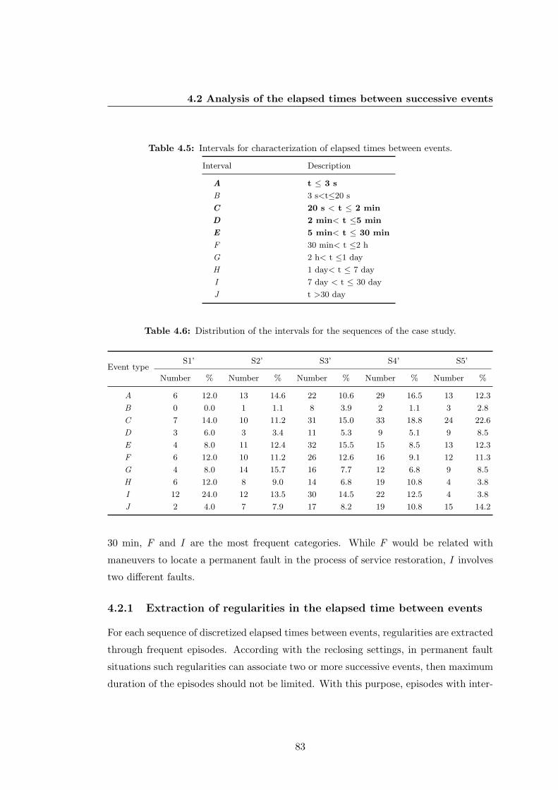
4.2 Analysis of the elapsed times between successive events
Table 4.5: Intervals for characterization of elapsed times between events.
Interval Description
A t ≤ 3 s
B 3 s<t≤20 s
C 20 s < t ≤ 2 min
D 2 min< t ≤5 min
E 5 min< t ≤ 30 min
F 30 min< t ≤2 h
G 2 h< t ≤1 day
H 1 day< t ≤ 7 day
I 7 day < t ≤ 30 day
J t >30 day
Table 4.6: Distribution of the intervals for the sequences of the case study.
Event typeS1’ S2’ S3’ S4’ S5’
Number % Number % Number % Number % Number %
A 6 12.0 13 14.6 22 10.6 29 16.5 13 12.3
B 0 0.0 1 1.1 8 3.9 2 1.1 3 2.8
C 7 14.0 10 11.2 31 15.0 33 18.8 24 22.6
D 3 6.0 3 3.4 11 5.3 9 5.1 9 8.5
E 4 8.0 11 12.4 32 15.5 15 8.5 13 12.3
F 6 12.0 10 11.2 26 12.6 16 9.1 12 11.3
G 4 8.0 14 15.7 16 7.7 12 6.8 9 8.5
H 6 12.0 8 9.0 14 6.8 19 10.8 4 3.8
I 12 24.0 12 13.5 30 14.5 22 12.5 4 3.8
J 2 4.0 7 7.9 17 8.2 19 10.8 15 14.2
30 min, F and I are the most frequent categories. While F would be related with
maneuvers to locate a permanent fault in the process of service restoration, I involves
two different faults.
4.2.1 Extraction of regularities in the elapsed time between events
For each sequence of discretized elapsed times between events, regularities are extracted
through frequent episodes. According with the reclosing settings, in permanent fault
situations such regularities can associate two or more successive events, then maximum
duration of the episodes should not be limited. With this purpose, episodes with inter-
83

4. MINING VOLTAGE DIP SEQUENCES RECORDED IN POWERDISTRIBUTION SUBSTATIONS
Figure 4.4: Histogram of elapsed time between consecutive events.
event time constraint (Definition 2.12) are extracted using the algorithm proposed in
Section 2.4.
Given that each element in the sequence S’ was obtained from timestamps of consec-
utive events, a maximal gap of 1 and 2 elements is used in the search. Likewise, several
minimum frequency (min fr) values were tested. Episodes related with settings of the
protective system were obtained using min fr values no greater than 4, 5, 10, 9 and 7
for the sequences S1’ to S5’, respectively. The frequency of relevant intervals of each
sequence (see Table 4.6) can be used as a guide for setting the threshold frequency of
frequent episodes. So, for example in the sequence S1’, interval A or C have frequen-
cies of 6 and 7 occurrences, respectively, then episodes –with length greater than one
event– that involve any of these two intervals must have min fr values less than 6 or
7, respectively.
Table 4.7 shows the frequent episodes (length greater than 1) for each sequence and
the two values of maximal gap (1 and 2 elements) are used. In this table, it can be
observed that episode 〈A,C〉 is frequent in all sequences analysed. This episode involves
the two intervals containing the automatic reclosing settings of the protective system.
Its frequency is about the number of permanent faults (permanent faults causing three
or more voltage dips) when a maximal gap of two elements is used.
Using maximal gap of two elements, episodes 〈A,C,C〉 for sequence S4’, 〈A,C, F 〉
84

4.2 Analysis of the elapsed times between successive events
Table 4.7: Frequent episodes and number of occurrences in the sequences for two valuesof maximal gap.
EpisodeMaximal gap=1 Maximal gap=2
S1’ S2’ S3’ S4’ S5’ S1’ S2’ S3’ S4’ S5’
〈A,C〉 5 7 14 15 9 5 8 15 18 18
〈C,C〉 10 10
〈C,E〉 5 10
〈C,F 〉 15 9 9
〈C,G〉 5
〈E,E〉 10
〈E, I〉 10
〈E, J〉 7
〈F,E〉 11
〈F,G〉 5
〈G,A〉 6
〈H, I〉 4 5
〈I, A〉 5 5 10 10 10
〈I, I〉 4
〈J,A〉 10 9 9
〈J,C〉 9
〈A,C,C〉 9
〈A,C,E〉 5
〈A,C, F 〉 10
〈J,A,C〉 7
for sequences S3’ and 〈A,C,E〉 for sequence S2’, are frequents. These episodes include
manual reclosing times and suggest that correspond to permanent faults causing at
least four voltages dips. Episodes such as 〈C,F 〉, 〈C,G〉, 〈E,E〉, 〈E, I〉 and 〈E, J〉,include manual reclosing times and suggest that these manoeuvres are frequent in these
substations but with different operating times. Episodes such as 〈I, A〉 are frequent in
sequences S2’ to S5’ or 〈J,A〉 are frequent in sequences S3’ to S5’, which show that after
several days (more than 30 days) of the occurrence of an event, new faults (causing
at least two voltage dips) usually occur. Episode 〈J,A,C〉 frequent in S5’ shows that
after several days without events (more than 30 days), new faults causing at least three
voltage dips usually occur. Finally, episodes such as 〈H, I〉 or 〈I, I〉 which are frequent
in sequence S4’, show the occurrences of several successive events associated to different
fault situations.
85

4. MINING VOLTAGE DIP SEQUENCES RECORDED IN POWERDISTRIBUTION SUBSTATIONS
4.2.2 Significant regularities in the elapsed time between events
Frequent episodes found in the previous section (Table 4.7) are evaluated using def-
initions and indexes described in Section 3.3. So, the strength of the link between
the different elapsed times contained in each episode is evaluated from their cohesion,
confidence and backward-confidence values, and the most significant associations are
identified.
Using a maximal gap of two elements, Table 4.8 contains for each episode, the
corresponding serial and parallel frequencies and the values of cohesion, confidence and
backward-confidence indexes.
According to Table 4.8 all frequent episode have a cohesion greater than 0.7, i.e.,
the order relation expressed by the serial episodes is strong. Episode 〈A,C〉 occurs with
a confidence greater than 0.6 in all sequences. This episode shows that if two successive
voltage dips have a elapsed time less than 3 s, one may expect with a confidence greater
than 0.6 (0.83, 0.62, 0.68, 0.62 and 0.77 for S1’ to S5’, respectively) that there will be
a third event within 20 s to 120 s of the second one.
Episodes 〈A,C,C〉 (for S4’), 〈A,C,E〉 (for S2’) and 〈A,C, F 〉 (for S3’), which are
forward-extensions (see Section 2.3.1.3) of the episode 〈A,C〉, have confidences greater
than 0.5. These episodes show that at least half of the occurrences of an episode 〈A,C〉(described above) are followed by a fourth event within 20 s to 120 s and 5 min to 30
min of the third one, respectively.
Finally, episodes 〈A,C〉 for S1’, 〈A,C,E〉 for S2’, 〈A,C, F 〉 for S3’, 〈A,C,C〉 for S4’
and 〈J,A,C〉 for S5’, are the maximal episodes with higher values (> 0.5) of cohesion,
confidence and backward-confidence. They are the most relevant pattern in these se-
quences. However, the pattern 〈A,C〉 have significant vales of cohesion and confidence
in all sequences analysed. This pattern involves the two intervals containing the auto-
matic reclosing settings of the protective system, therefore it may identified permanent
faults that cause at least three successive voltage dips.
Figures 4.5 to 4.9 show for each sequence, the episodes selected as patterns. They
are marked by a dashed line between circular marks (green circular marks for episode
〈A,C〉 and red circular marks for their extensions). At the top of the figures, the
sequences of elapsed times between events and the corresponding patterns are shown,
while in the bottom of the figures, it adds information about the events in the sequence.
86

4.2 Analysis of the elapsed times between successive events
Table 4.8: Frequent episodes and their corresponding values of of cohesion (coh), confi-dence (conf) and backward-confidence (confB).
Sequence Episode fr(α) fr(αp) coh confB conf
S1’
〈A,C〉 5 5 1.00 0.71 0.83
〈H, I〉 4 4 1.00 0.33 0.67
〈I, I〉 4 4 1.00 0.33 0.33
S2’
〈A,C〉 8 8 1.00 0.80 0.62
〈C,E〉 5 6 0.83 0.45 0.50
〈C,G〉 5 5 1.00 0.36 0.50
〈F,G〉 5 5 1.00 0.36 0.50
〈G,A〉 6 6 1.00 0.46 0.43
〈H, I〉 5 6 0.83 0.42 0.63
〈I, A〉 5 7 0.71 0.38 0.42
〈A,C,E〉 5 6 0.83 1.00 0.63
S3’
〈A,C〉 15 15 1.00 0.48 0.68
〈C,E〉 10 12 0.83 0.31 0.32
〈C,F 〉 15 17 0.88 0.58 0.48
〈E,E〉 10 10 1.00 0.31 0.31
〈E, I〉 10 13 0.77 0.33 0.31
〈F,E〉 11 14 0.79 0.34 0.42
〈I, A〉 10 12 0.83 0.45 0.33
〈J,A〉 10 10 1.00 0.45 0.59
〈A,C, F 〉 10 11 0.91 0.67 0.67
S4’
〈A,C〉 18 19 0.95 0.55 0.62
〈C,C〉 10 10 1.00 0.30 0.30
〈C,F 〉 9 9 1.00 0.56 0.27
〈I, A〉 10 11 0.91 0.34 0.45
〈J,A〉 9 10 0.90 0.31 0.47
〈A,C,C〉 9 11 0.82 0.90 0.50
S5’
〈A,C〉 10 10 1.00 0.42 0.77
〈C,F 〉 9 11 0.82 0.75 0.38
〈E, J〉 7 8 0.88 0.47 0.54
〈J,A〉 9 9 1.00 0.69 0.60
〈J,C〉 9 10 0.90 0.38 0.60
〈J,A,C〉 7 7 1.00 0.70 0.78
This information indicates which events are caused by permanent or transient faults
and which of them are no documented events.
A comparison of the results in Fig. 4.5 with the information in Table 4.3 confirms
that acting times during manual operation are not performed strictly in this sequence.
87

4. MINING VOLTAGE DIP SEQUENCES RECORDED IN POWERDISTRIBUTION SUBSTATIONS
Figure 4.5: Sequence S1’ and occurrences of the episode 〈A,C〉.
This is probably because manual actuations are related to fault location strategies
followed in each situation. Moreover, there is a permanent fault (〈e22, e23, e24〉) that
does not follow the pattern. A possible interpretation is the involvement of secondary
protections such as fuses, or that the fault was caused by another abnormal situation,
not considered in the studied pattern.
Finally, in order to assess the identification of permanent fault situations by the
episode 〈A,C〉 shown in Figures 4.5 to 4.9 the following parameters are used: number
of permanent faults correctly identified or true detection (TD), permanent faults not
detected or missed by detection (MD) and, number of non permanent faults identified
as permanent or false alarms (FA). The corresponding ratios also included in Table
4.9 are useful to evaluate the accuracy of the search: true detection rate (TDR =
TD/(TD+MD)), missed detection rate (MDR = MD/(TD+MD)) and false alarm rate
(FAR = FA/(TD+FA)). The results are summarised in Table 4.9.
For sequences S1’ to S5’, TDR values indicate that 83%, 100%, 76%, 86% and 80%
of permanent faults with more than three events follow the automatic reclosing pattern
of the protective system, respectively. However, the pattern can not be found in some
situations, for example, when a single event is enough to detect or locate the failure or
when a secondary protection acts. An accurate analysis discovered that the high value
88

4.2 Analysis of the elapsed times between successive events
Figure 4.6: Sequence S2’ and occurrences of episodes 〈A,C〉 and 〈A,C,E〉.
Figure 4.7: Sequence S3’ and occurrences of episodes 〈A,C〉 and 〈A,C, F 〉.
of FAR in S2’, S3’ and S5 was due to the fact that the episode 〈A,C〉 was detected in
no documented events. Also, the high value MDR in S3’ and S4’ was due to the fact
that the first automatic reclosing was not recorded for several permanent faults.
89

4. MINING VOLTAGE DIP SEQUENCES RECORDED IN POWERDISTRIBUTION SUBSTATIONS
Figure 4.8: Sequence S4’ and occurrences of episodes 〈A,C〉 and 〈A,C,C〉.
Figure 4.9: Sequence S5’ and occurrences of episodes 〈A,C〉 and 〈J,A,C〉.
90
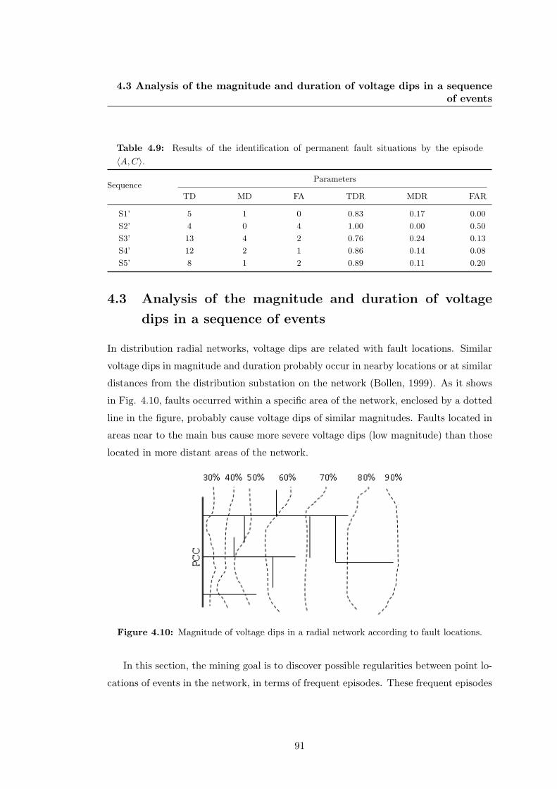
4.3 Analysis of the magnitude and duration of voltage dips in a sequenceof events
Table 4.9: Results of the identification of permanent fault situations by the episode〈A,C〉.
SequenceParameters
TD MD FA TDR MDR FAR
S1’ 5 1 0 0.83 0.17 0.00
S2’ 4 0 4 1.00 0.00 0.50
S3’ 13 4 2 0.76 0.24 0.13
S4’ 12 2 1 0.86 0.14 0.08
S5’ 8 1 2 0.89 0.11 0.20
4.3 Analysis of the magnitude and duration of voltage
dips in a sequence of events
In distribution radial networks, voltage dips are related with fault locations. Similar
voltage dips in magnitude and duration probably occur in nearby locations or at similar
distances from the distribution substation on the network (Bollen, 1999). As it shows
in Fig. 4.10, faults occurred within a specific area of the network, enclosed by a dotted
line in the figure, probably cause voltage dips of similar magnitudes. Faults located in
areas near to the main bus cause more severe voltage dips (low magnitude) than those
located in more distant areas of the network.
Figure 4.10: Magnitude of voltage dips in a radial network according to fault locations.
In this section, the mining goal is to discover possible regularities between point lo-
cations of events in the network, in terms of frequent episodes. These frequent episodes
91

4. MINING VOLTAGE DIP SEQUENCES RECORDED IN POWERDISTRIBUTION SUBSTATIONS
can show relationships between a fault and other faults occurred at the same or an-
other location on the network. Two different interpretations can be derived from such
episodes:
1. Frequent episodes composed by multiple and similar (magnitude an duration)
events will represent areas of the network susceptible to the occurrence of succes-
sive faults.
2. Frequent episodes composed by events of different magnitudes could show inter-
actions between faults located in different regions of the network.
4.3.1 Dataset description
A set of voltage dips caused by single-phase faults are analysed. Events, recorded as
shown in Section 4.1.1, correspond to a substation with a high rate of events.
Voltage dip density tables is a common method for presenting large repositories (or
surveys) of dips gathered during long periods of time (more than one year). There are
several proposed tables (Yuan et al., 2009). We use the table recommended by the
standard IEC61000-2-8 (2002). In this table, magnitude of dips is split in 9 categories
defined by the following intervals: 80%–90%, 70%–80%, 60%–70%, 50%–60%, 40%–
50%, 30%–40%, 20%–30%, 10%–20% and <10%. For the dips duration, 8 intervals are
used: <0.1s, 0.1s–0.25s, 0.25s–0.5s, 0.5s–1s, 1s–3s, 3s–20s, 20s–60s and 60s–180s.
The analyzed data set is represented in Table 4.10. It contains a total of 527 voltage
dips recorded during a monitored period of three years.
Duration intervals are represented by a 8-letter alphabet (A to F), while numbers
1 to 9 are used to represent the magnitude intervals. Each voltage dip in the sequence
is represented by their corresponding identifier of row and column in Table 4.10. For
example, the voltage dip type B6 represents dips with duration between 0.1s to 0.25s
and magnitude between 50% to 60% while the voltage dip type D3 represents dips with
duration between 0.5s to 1s and magnitude between 20% to 30%. So, the sequence can
have 72 different types of events. Likewise, H1 will be the most severe voltage dips,
while A9 will be the less severe.
Fig. 4.11 shows the distribution of the cumulated number of voltage dips according
with the classification of Table 4.10. This figure shows that the sequence has only 36
of 72 possible voltage dip types. B6 with around of 10% of the events is the most
92

4.3 Analysis of the magnitude and duration of voltage dips in a sequenceof events
Table 4.10: Cumulative voltage dip table.
Magnitude
Duration
A B C D E F G H
<0.1 s 0.1–0.25 s 0.25–0.5 s 0.5–1 s 1–3 s 3–20 s 20–60 s 60–180 s
9 80%–90% 4 3 1 2 4 0 0 0
8 70%–80% 4 6 11 2 4 0 0 0
7 60%–70% 1 42 28 4 15 1 0 0
6 50%–60% 0 55 39 8 9 0 0 0
5 40%–50% 0 28 13 10 17 0 0 0
4 30%–40% 1 21 20 32 25 4 0 0
3 20%–30% 0 5 5 39 13 0 0 0
2 10%–20% 0 0 38 14 0 0 0 0
1 <10% 0 0 0 0 0 0 0 0
frequent voltage dip type in the sequence, followed by B7 with around of 8% of the
events. Likewise, C2, C6 and D3, each one with around of 7% of the events, have
similar frequencies in the sequence.
Figure 4.11: Distribution of the voltage dips according to magnitude and duration.
93

4. MINING VOLTAGE DIP SEQUENCES RECORDED IN POWERDISTRIBUTION SUBSTATIONS
4.3.2 Frequent regularities between points of occurrence of events in
the network
As it was introduced in this section, the main interest for the extraction of frequent
episodes in sequences of voltage dips is to find relations between fault location areas.
So, in the mining process, it is only necessary to consider one voltage dip for each
fault occurred in the network. However, as shown in Section 4.2 several events close in
time can be generated for the same fault. This problem can be partially solved using
temporal aggregation (Bollen, 1999). If several voltage dips occur within a time interval
less than a predefined time of aggregation, then the aggregated event could be defined
by one of the following options:
1. The time between the start of the first event and the end of the last event, and
the residual voltage of the first event.
2. The sum of the individual durations and the minimal residual voltage of the
events.
3. The duration and the residual voltage of the first event.
4. The maximal duration and the minimal residual voltage of the events.
Option 3 is the most appropriate to include the behavior of all events in the analysis
of the sequence without changing the information contained in the event. Likewise,
considering observations in Section 4.2, 2 hours can be used as time of aggregation.
Algorithm Fminevent proposed in Section 2.4 is used for the search of frequent
episodes. With this algorithm, temporal aggregation can be included by using a time
interval, (tmin tmax] for the inter-event time constraint between events of the episodes as
shown in Section 2.4.1.2. For a candidate episode, successive events with elapsed times
less than tmin, are not considered for their occurrences. So, tmin serves as aggregation
time, reducing the effects of multiples events of the same fault.
Fig 4.12 shows the number of frequent episodes discovered in the sequence for several
values of minimum frequency threshold (min fr) and for several values of maximal gap
between events (tmax). This results are obtained using a tmin value of 2 hours.
Fig. 4.12a shows wide differences between the number of episodes obtained with
min fr = 4 (occurrences) and min fr = 6 (occurrences) for the same value of tmax.
94

4.3 Analysis of the magnitude and duration of voltage dips in a sequenceof events
(a) Several values of min fr (occurrences)
(b) Several values of tmax (days)
Figure 4.12: Number of frequent episodes for several values of min fr and maximal gapbetween events (tmax)
95

4. MINING VOLTAGE DIP SEQUENCES RECORDED IN POWERDISTRIBUTION SUBSTATIONS
For example, for tmax = 8 days, the number of frequent episodes is reduced from 100
to 30 for min fr = 4 and min fr = 6, respectively. For min fr values greater than 6
occurrences, there are minor differences in the number of frequent episodes. Likewise,
for different values of tmax, Fig. 4.12b show that few frequent episodes are obtained
for min fr values greater than 8 occurrences.
Fig. 4.13 shows a schema of frequent episodes with min fr = 6 occurrences and
tmax = 8 days. Two-event and three-event episodes are linked by thin and thick arrows,
respectively. For this sequence, these frequent episodes suggest the presence of regular-
ities between events of the same region (episodes with two or more events of the same
type) and between events of different regions (episodes with events of different types).
Most of them are episodes of two-event length and only 4 episodes have three-event
length. They are: 〈B4, B4, D3〉, 〈B5, B4, D3〉, 〈B4, C4, D3〉 and 〈C2, C2, C2〉 which
are highlighted in the figure. Several episodes are composed of events C6 and D3
(linked by a thin orange and black arrow in the figure, respectively)and many of them
end with event D3. In these episodes, the most severe voltage dips (lowest magnitude)
correspond to events C2 and D3 while the less severe are B7 and C7.
Figure 4.13: Representation of frequent episodes with min fr = 6 occurrences and tmax
= 8 days.
Most frequent episodes in Fig. 4.13, show that the first event is greater in magnitude
than later events or they are associated to voltage dips similar in magnitude. Table
96

4.3 Analysis of the magnitude and duration of voltage dips in a sequenceof events
4.11 contain the list of frequent episodes grouped by their frequency which are between
6 to 13 occurrences.
Table 4.11: List of frequent episodes with min fr = 6 (occurrences) and tmax = 8 (days).
Episodes Frequency
〈B4, B4, D3〉; 〈B4, C4, D3〉, 〈B5, B4〉, 〈B5, B4, D3〉, 〈B5, B5〉, 〈B5, C7〉, 〈B7, E5〉,〈C2, C2, C2〉, 〈C5, D3〉, 〈C6, B4〉, 〈C6, D4〉, 〈D3, B4〉, 〈D3, B7〉, 〈D4, C7〉, 〈D4, D3〉,〈E3, C6〉, 〈E5, B6〉
6
〈B4, B4〉, 〈B5, C5〉, 〈B5, C6〉, 〈B5, D3〉, 〈B6, B7〉, 〈B6, E5〉, 〈B7, C6〉, 〈C2, D4〉,〈C6, C2〉, 〈D3, D3〉, 〈D4, C2〉, 〈D4, D4〉, 〈E4, B4〉
7
〈B4, C4〉, 〈C2, D3〉, 〈C4, D3〉, 〈C6, B6〉, 〈D3, C4〉 8
〈B4, D3〉, 〈B7, B7〉, 〈C6, C6〉, 〈D3, C6〉 9
〈B6, B6〉, 〈B6, C6〉, 〈C6, D3〉 10
〈B7, B6〉, 〈D3, D4〉 11
〈C2, C2〉 13
〈C2, C2〉 is the most frequent event with 13 occurrences while the 4 episodes with
three-event length have 6 occurrences.
4.3.3 Significant regularities between points of occurrence of events
in the network
Frequent episodes in Table 4.11 are evaluated starting from their corresponding values
of cohesion, confidence and backward-confidence. For these indexes, Fig. 4.14 shows
the distribution of the number of frequent episodes. Only two episodes have cohesion
values lower than 0.5, i.e, most of them follow a serial order in the sequence. In contrast,
for confidence and backward-confidence, only 7 and 5 episodes have values grater than
0.4, respectively. Then, only few episodes have relevant probabilities of apparition in
the sequence.
Table 4.12 shows frequent episodes which values of cohesion (coh), confidence (conf)
and backward-confidence (confB) are greater than 0.4.
Episode 〈B4, B4, D3〉 shown in Table 4.12, relates two type of events. B4 represents
voltage dips with magnitude of 30%–40% and 0.1–0.25 s of duration, and D3 represents
voltage dips with 20%–30% in magnitude and 0.5–1 s of duration. According to their
97

4. MINING VOLTAGE DIP SEQUENCES RECORDED IN POWERDISTRIBUTION SUBSTATIONS
Figure 4.14: Number of frequent episodes according to their values of cohesion (coh),confidence (conf) and backward-confidence (confB).
Table 4.12: Significant episodes and their corresponding values of of cohesion (coh),confidence (conf) and backward-confidence (confB).
Episode fr(α) fr(αp) coh confB conf
〈B4, B4, D3〉 6 6 1.00 0.67 0.86
〈B4, C4, D3〉 6 8 0.75 0.75 0.75
〈B5, B4, D3〉 6 7 0.86 0.67 1.00
〈C2, C2, C2〉 6 6 1.00 0.46 0.46
magnitudes, D3 is more severe than B4, which suggests that D3 represents voltage
dips located closer to the main bus of the distribution network (substation), than those
represented by B4. Fig. 4.15 shows occurences of episode 〈B4, B4, D3〉 along the
sequence, marked by a dashed line between red circular marks. Occurrences of their
prefix (episode 〈B4, B4〉) are also highlighted in the figure by blue circular marks.
According to this figure, 6 of 7 occurrences of 〈B4, B4〉 also comprise occurrences of
〈B4, B4, D3〉. Two of these occurrences appear at the beginning of the sequence, two
at the center and two at the end.
Episode 〈B4, C4, D3〉 shown in Table 4.12, combines three type of events. B4 rep-
98

4.3 Analysis of the magnitude and duration of voltage dips in a sequenceof events
Figure 4.15: Sequence of voltage dips and occurrences of episodes 〈B4, B4〉 and〈B4, B4, D3〉.
resents voltage dips with magnitude of 30%–40% and 0.1–0.25 s of duration, C4 are
voltage dips with same magnitude of B4 and 0.25–0.5 s of duration and D3 represents
voltage dips with 20%–30% in magnitude and 0.5–1 s of duration. According to their
magnitudes and durations, D3 is more severe than C4 and C4 is more severe than B4,
which suggest that D3 represent voltage dips located closer to the main bus of the
distribution substation, than those represented by C4, while B4 represent voltage dips
located in similar areas than C4. Occurences of this episode along the sequence are
shown in Fig. 4.16, marked by a dashed line between red circular marks. Figure also
shows occurrences of their prefix (episode 〈B4, C4〉) by blue circular marks. Accord-
ing to this figure, occurrences of 〈B4, C4, D3〉 are derived from 6 of 8 occurrences of
〈B4, C4〉. Two of these occurrences appear at the beginning of the sequence, one at
the center and three at the end. Occurrences of B4 and D3 of this episode are also
involved in episode 〈B4, B4, D3〉 shown in Fig. 4.15.
Episode 〈B5, B4, D3〉 shown in Table 4.12, combines three type of events. B5
represents voltage dips with magnitude of 40%–50% and 0.1–0.25 s of duration, B4
are voltage dips with 30%–40% of magnitude and the same duration as B5, and D3
represents voltage dips with 20%–30% in magnitude and 0.5–1 s of duration. According
99

4. MINING VOLTAGE DIP SEQUENCES RECORDED IN POWERDISTRIBUTION SUBSTATIONS
Figure 4.16: Sequence of voltage dips and occurrences of episodes 〈B4, C4〉 and〈B4, C4, D3〉.
to their magnitudes and durations, D3 is more severe than B4 and B4 is more severe
than B5, which suggests that D3 represents voltage dips located closer to the main bus
of the distribution network, than those represented by B4, while B5 represents voltage
dips located further than the B4. Occurences of this episode along the sequence are
shown in Fig. 4.17, marked by a dashed line between red circular marks. Figure also
shows occurrences of their prefix (episode 〈B5, B4〉) by blue circular marks. According
to this figure, occurrences of 〈B5, B4, D3〉 are derived from the same occurrences of
〈B5, B4〉. Three of these occurrences appear at the beginning of the sequence, and the
remaining three at the end. Occurrences of B4 and D3 of this episode are also involved
in episodes 〈B4, B4, D3〉 (Fig. 4.15) and 〈B4, C4, D3〉 (Fig. 4.16).
Episode 〈C2, C2, C2〉 relates voltage dips with 10%–20% in magnitude and duration
of 0.25–0.5 s. This episode suggests the recurrence of fault close in time, located on
the same network zone. Occurences of this episode along the sequence are shown in
Fig. 4.18, marked by a dashed line between red circular marks. Figure also shows
occurrences of their prefix (episode 〈C2, C2〉) by blue circular marks. occurrences of
〈C2, C2, C2〉 appear only at the beginning of the sequence.
100

4.3 Analysis of the magnitude and duration of voltage dips in a sequenceof events
Figure 4.17: Sequence of voltage dips and occurrences of episodes 〈B5, B4〉 and〈B5, B4, D3〉.
Figure 4.18: Sequence of voltage dips and occurrences of episodes 〈C2, C2〉 and〈C2, C2, C2〉.
101
4. MINING VOLTAGE DIP SEQUENCES RECORDED IN POWERDISTRIBUTION SUBSTATIONS
4.4 Conclusions
Sequences of voltage dips recorded in a power distribution network were analysed in
order to find causal associations between events. Two types of regularities were dis-
covered in this sequences. The first one involves the elapsed time between voltage dip
events, while the second associates voltage dips starting from their magnitudes and
durations.
Elapsed times between voltage dip events can show reclosing settings of the protec-
tive system. In power distribution networks, protective system usually have scheduled
two automatic reclosing for clearing a fault. For the sequences studied in this work, re-
sults show that over 60% of the occurrences of the first automatic reclosing are followed
by a second automatic attemp. Likewise, for over 80% of permanent faults (single-phase
faults), the two automatic reclosing attempts are performed.
Magnitude and duration of voltage dips reflect the fault location in the network.
Network areas prone to fault occurrences can be found from frequent episodes composed
by similar voltage dips closed in time. Also, possible causal interactions between faults
of the network could be found from frequent episodes composed by several events.
These two situations were observed in the analysed sequence. Most frequent episodes
found are associated to voltage dips similar in magnitude or they indicate that early
events are larger in magnitude than subsequent events. These frequent episodes may
show that early events influence the occurrences of subsequent events.
The mining algorithm –Fminevent– developed in Section 2.4, is suitable for the
analysis of these sequences of voltage dips. It is able to determine the frequency of
episodes without missing or over-counting occurrences. According to the criteria de-
veloped in the Section 3.3, serial and parallel frequency values of an episode are key
to assess its significance. Nevertheless, each sequence must be analyzed individually
to establish the most appropriate parameters related to the threshold frequency and
duration of episodes.
102

5
Pattern discovery in sequences of
incidents collected in power
distribution networks
Incidents registered in power distribution networks are analysed in this chapter. Util-
ities use the term incident to indicate the existence of faults or situations that affect
the continuity of supply. They are recorded from customer service centers or incidents
management systems. Each incident is documented with different attributes such as the
occurring date, its cause and its duration. Mining algorithm proposed in Section 2.4
is adapted for the discovery of order relations between main causes of incidents on the
network. Methods developed in Chapter 3 are used to identify significant associations
between these incidents cause and their physical meaning is discussed.
5.1 Introduction
Environmental conditions, external agents (animals, vegetation, vehicles, etc.) or aging
of components are factors that affect the frequency of occurrence of faults and failures in
the network. Moreover, depending on the severity of faults, protective systems are auto-
matically fired, affecting continuity and quality of supply in different manner. Utilities
usually use the term incident to indicate the existence of such misbehaviours (faults and
failures) that affect the continuity of supply and are systematically reported together
with the activity performed to restore the normal operation of the system (reparation,
103

5. PATTERN DISCOVERY IN SEQUENCES OF INCIDENTSCOLLECTED IN POWER DISTRIBUTION NETWORKS
material substitution, fuse replacement, etc.) (ECO/797/2002, 2002). Examples of
incidents are failures in cables produced by moisture or aging and its corresponding
reparation, the actuation of protective system in the head of a feeder in presence of
lightning followed by a restoration sequence or the automatic reclosing after a branch
tree contact in a windy day.
If incidents recorded in a feeder or sector of the distribution network are sorted as
a sequence of incidents then the existence of order relations between them can be dis-
covered. The analysis involves the application of frequent episode discovery algorithms
as well as the evaluation of the relevance of episodes found. We focus the search on
short-term episodes that is set of incidents occurring with a time difference less than a
fixed expiry-time, while their inter-event time is not constrained. Episodes that contain
representative types of incidents can be identified and the analysis of the occurrence
causes can be performed.
5.2 Dataset description
The dataset of incidents available in this research were collected over three years in a
real power system by the utility from customer service centers or incidents manage-
ment systems. Each incident was documented with the occurring date, the main cause
(storm, tree, component failure, etc.) and the voltage level where it was originated
(medium voltage MV, low voltage LV, etc). Table 5.1 shows a short description of each
cause and an alphabet of 15 letters is used to typify each one of them.
Five feeders with large number of incidents were selected for the case study. The
incidents occurred in each one of the feeders were analyzed as single sequences and
each incident is represented with two attributes: its cause and its corresponding time
of occurrence. In case of an incident does not correspond to an interruption of the
supply, the corresponding lowercase letter is used. The distribution of the incidents in
the five feeders is shown in Table 5.2.
Table 5.2 shows that more than 50% of incidents were caused by unknown causes
(f) and they did not originate interruptions in the power supply. For the feeder 1,
vandalism (Q) was the second most common cause of fault. In feeder 2 and feeder
5 around 1% of the incidents correspond to component breakdown (H) while in the
other feeders, this incident type represents more than 5% of the incidents. Also, feeder
104

5.3 Order relations between main causes of network incidents
Table 5.1: Types of causes and short description.
Type Description Type Description
A animals J cable falls to ground
B trees K fuse
C storm/lightning L live-line work
D wind M contractor personnel
E rain N individuals
F unknown O excavations
G overload P vehicles
H component breakdown Q vandalism
I handling to restore supply R private facilities
T customer connection
Lowercase letters are used when the incident did not cause interruptions (punishable) of supply.
2 and feeder 5 are the most afected by incidents originated in private facilities (R)
and incidents with unkown cause (f and F ). Feeder 1, feeder 3 and feeder 5 are the
most afected by incidents related with supply restoration (i), while feeder 4 is the most
afected by melted fuse (K).
5.3 Order relations between main causes of network inci-
dents
For each sequence described in Table 5.2 the frequent episodes are extracted. We focus
the search on short-term episodes that are composed by incidents that occurred with a
time difference less than the expiry-time, then their inter-event time is not constrained.
Frequent episodes are obtained using the mining algorithm Fminevent proposed in
Sections 2.4 and 2.4.1.1.
Fig. 5.1 shows for each feeder the number of frequent episodes for several values of
expiry-time Tx (between 1 and 20 days) using a min fr = 4 occurrences. An inter-event
time constraint equal to the expiry-time Tmax = Tx is used for each case.
According to these results, although the sequences of the case study are short se-
quences, a huge number of frequent episodes are found. This number increases as the
time-expiry constraint increases. The number of frequent episodes in feeder 1 and feeder
2 show a similar trend until Tx = 15 days, and then both grow exponentially. Feeder
3, 4 and 5 show a similar linear trend for all Tx.
105

5. PATTERN DISCOVERY IN SEQUENCES OF INCIDENTSCOLLECTED IN POWER DISTRIBUTION NETWORKS
Table 5.2: Types and number of incidents for each feeder in the case study.
TypeFeeder 1 Feeder 2 Feeder 3 Feeder 4 Feeder 5
Number % Number % Number % Number % Number %
A 3 1.36 1 0.52
B 1 0.36 1 0.36
C 3 1.09 2 0.90 3 1.55 3 1.59
c 1 0.36 3 1.09 1 0.45 2 1.03 1 0.53
D 1 0.45 2 1.03 1 0.53
d 1 0.36 1 0.45 3 1.55 3 1.59
E 2 0.73 2 0.90
e 2 0.90
F 12 4.35 28 10.22 11 4.98 12 6.19 4 2.12
f 150 54.35 198 72.26 155 70.14 117 60.31 151 79.89
g 1 0.36
H 14 5.07 3 1.09 16 7.24 11 5.67 2 1.06
h 5 1.81 2 0.90 1 0.52
I 5 1.81 3 1.09 6 2.71 3 1.55 1 0.53
i 24 8.70 3 1.09 9 4.07 4 2.06 8 4.23
J 1 0.45
K 3 1.09 1 0.45 10 5.15 3 1.59
k 1 0.36 1 0.52
L 4 2.06
l 3 1.09 6 3.09
M 2 0.72
N 1 0.36
n 1 0.36
P 1 0.36 3 1.55 1 0.53
Q 49 17.75 1 0.36
q 6 2.17
R 2 0.72 19 6.93 8 3.62 8 4.12 11 5.82
r 2 0.73 2 1.03
t 1 0.36 1 0.52
Total 276 274 221 194 189
λ1 0.25 0.25 0.20 0.18 0.17
1 Average rate of incidents per day.
Likewise, Fig. 5.2 shows the number of frequent episodes varying the minimum
frequency threshold for a fixed time-expiry of 15 days. Selection of this time-expiry is
reinforced by the behaviours of feeders 1 and 2 observed in Fig. 5.1. The exponential
grow in the number of frequent episodes seems to be given by the random combination
106

5.3 Order relations between main causes of network incidents
Figure 5.1: Number of frequent episodes found in each feeder for several values of expiry-time, min fr = 4 occurrences.
of independent and frequent causes of incidents. The objective is to identify frequent
episodes that are not given by random combination of frequent causes of incidents, but
specific situations linked to the ordered occurrence of the incidents in the episode. Fig.
5.2 shows, for each feeder, that the number of frequent episodes decreases exponentially
as the threshold (min fr) increases. The plot suggests a threshold for feeder 1 and 2
around min fr = 4 while for feeder 3, 4 and 5 is around min fr = 3. From these values
further, the number of frequent episodes that are found stabilizes with independence
of the threshold.
As it occurs with the time-expiry constraint, the maximal gap between events (inter-
event time constraint) influences on the number of occurrences found for each episode
and also on the total number of frequent episodes. So, if the maximal gap between
incidents increases also the number of frequent episodes increases. Table 5.3 shows
the total number of frequent episodes discovered in the sequences for several values of
maximal gap using a time-expiry constraint of 15 days. In the table these maximal
gaps are expressed as fractions of time-expiry, 0.2, 0.4, 0.6, 0.8 and 1, which are equals
to 3, 6, 9, 12 and 15 days, respectively. According to the observations in Fig. 5.2, two
minimum threshold were used: min fr = 4 for feeder 1 and 2 and min fr = 3 for
feeder 3, 4 and 5.
107

5. PATTERN DISCOVERY IN SEQUENCES OF INCIDENTSCOLLECTED IN POWER DISTRIBUTION NETWORKS
Figure 5.2: Number of frequent episodes found in each feeder for several values of min frand Tx = 15 days.
Table 5.3: Number of frequent episodes found in the sequences for several values ofmaximal gap.
SequenceMaximal gap as fraction of the expiry-time Tx = 15 days
0.2 0.4 0.6 0.8 1
Feeder1 1 60 143 209 235 260
Feeder2 1 67 151 201 212 217
Feeder3 2 34 116 138 152 152
Feeder4 2 30 53 61 70 73
Feeder5 2 27 34 66 75 79
1 With 4 occurrences as minimum threshold.
2 With 3 occurrences as minimum threshold.
5.4 Significant order relations between main causes of net-
work incidents
According to the distribution of the incidents in the different feeders shown in Table 5.2,
the most frequent incidents are associated to unknown causes (type f), which means
that the majority of frequent episodes that are mined probably involve this type of
108
5.5 Relative location of the incidents within the frequent episodes
incident. However, this is an incident type that has not significant information. This
fact can mask other relevant episodes, less frequent but related with known causes. So,
excluding the incident type f in the candidate generation step (see Section 3.2.3.1) and
using min fr = 4 for feeder 1 and 2 and min fr = 3 for feeder 3, 4 and 5, the number
of frequent episodes (last column of Table 5.3) are reduced to 31, 6, 10, 13 and 7 for
each feeder, respectively. This number represent less than 10% of the total frequent
episodes found when the incident f was included in the search. Table 5.4 shows the
maximal frequent episodes (Definition 3.3) for each feeder avoiding the influence of the
incident type f .
Table 5.4 contains for each episode the corresponding values of cohesion, confidence
and backward-confidence indexes, which are calculated from the definitions in Chapter
3. If the episodes with higher value indexes (> 0.5) in this cited parameters are con-
sidered as patterns, then only the episodes 〈i,H, i〉 for feeder 1 and 〈F, F, F 〉 for feeder
2 could be extracted. The pattern 〈i,H, i〉 shows that handling to restore the supply
i usually involves the breakdown of components H. The pattern 〈F, F, F 〉 shows that
successive incidents of unknown cause F (interruption of the supply of unknown cause)
are frequent. The plot of the occurrences of these patterns for each sequence is shown
in Fig. 5.3 and Fig. 5.4.
Likewise, it can be observed that in three feeders (1, 3 and 4) where incidents caused
by components breakdown H were frequent, the episode 〈F,H〉 also was frequent. This
relation shows that incidents caused by component breakdown usually are preceded by
an interruption of the supply of unknown cause.
5.5 Relative location of the incidents within the frequent
episodes
An analysis of the relative location of the incidents within the frequent episodes is
presented in this section as a validation of the patterns found. The aim is to know if a
preferred location of certain types of incidents within the episodes exists. For example,
if the component breakdown usually is the final event of an episode or if unknown
incidents are the start events of the episodes. This analysis could help to establish
the most probably association that can perform an incident, i.e., if an incident has a
109

5. PATTERN DISCOVERY IN SEQUENCES OF INCIDENTSCOLLECTED IN POWER DISTRIBUTION NETWORKS
Table 5.4: Maximal frequent episodes (excluding the incident type f) and their corre-sponding values of of cohesion (coh), confidence (conf) and backward-confidence (confB).
Feeder Episode fr frp coh confB conf
1
〈i, I〉 4 4 1.00 0.80 0.17
〈i, F 〉 5 5 1.00 0.42 0.21
〈H, I〉 4 5 0.80 0.80 0.29
〈H,Q〉 6 9 0.67 0.12 0.43
〈h, i〉 4 5 0.80 0.17 0.80
〈Q,H〉 7 9 0.78 0.50 0.14
〈Q,F 〉 6 10 0.60 0.50 0.12
〈Q, q〉 4 5 0.80 0.67 0.08
〈F,H〉 4 4 1.00 0.29 0.33
〈F,Q〉 7 10 0.70 0.14 0.58
〈i, i, i〉 4 4 1.00 0.40 0.40
〈i, i,H〉 4 7 0.57 0.67 0.40
〈i, i, Q〉 5 8 0.63 0.45 0.50
〈i,H, i〉 4 7 0.57 0.80 0.67
〈i, Q, i〉 4 8 0.50 0.31 0.36
〈Q, i, i〉 5 8 0.63 0.50 0.38
〈Q,Q, i〉 4 7 0.57 0.31 0.24
〈Q,Q,Q〉 8 8 1.00 0.47 0.47
2
〈F,R〉 8 12 0.67 0.42 0.29
〈R,F 〉 6 12 0.50 0.21 0.32
〈F, F, F 〉 6 6 1.00 0.60 0.60
3
〈H, i〉 6 6 1.00 0.67 0.38
〈H,H〉 5 5 1.00 0.31 0.31
〈H, I〉 5 5 1.00 0.83 0.31
〈F,H〉 3 4 0.75 0.19 0.27
4〈K,K〉 3 3 1.00 0.30 0.30
〈F,H〉 3 3 1.00 0.27 0.25
5 〈R,R〉 3 3 1.00 0.27 0.27
forward or backward association with other frequent incidents in a sequence as it was
discussed in Section 3.2.3.
Whit this aim, for each incident type, the corresponding number of occurrences and
location within the episodes are counted and classified. Two main categories are used
to classify the location of each incident type: start or final event, percentage of total
occurrences where the incident is located at the beginning or end of the episodes and
110

5.5 Relative location of the incidents within the frequent episodes
Figure 5.3: Sequence of incidents of feeder 1 and occurrences of pattern 〈i,H, i〉 .
Figure 5.4: Sequence of incidents of feeder 2 and occurrences of pattern 〈F, F, F 〉 .
intermediate event, percentage of occurrences where the incident is located only in the
middle of the episode. Table 5.5 shows the evaluation of the relative position of the
incidents between the maximal frequent episodes, shown in Table 5.4. For example,
the incident by vandalism (Q) in the feeder 1, have 56 serial occurrences considering
the 10 maximal episodes where it appears. 92.9% of this ocurrences have Q as the first
111

5. PATTERN DISCOVERY IN SEQUENCES OF INCIDENTSCOLLECTED IN POWER DISTRIBUTION NETWORKS
or the final event, being the 60.7% the number of occurrences where it appears as the
first event, 7.1% of the occurrences it has a intermediate location, while 46.4% times
the incident appear as the last event of maximal episodes. The result would show that
incidents by vandalism Q could mainly trigger new incidents (the same or different
type).
In contrast, the incident type F (interruption of the supply of unknown cause) is
located at the beginning or at the end of the occurrences in similar proportion (50%).
Then, a role of this incident in the beginning or conclusion of episodes can not be
identified.
Table 5.5: Relative location of the incidents within the maximal frequent episodes.
Feeder Frequent
incidents
Maximal
Occurrences
Start or Final
event %
Start
event %
Final
event %
Only
intermediate
event %
1
Q 56 92.9 60.7 46.4 7.1
i 43 100.0 69.8 58.1 0.0
h 4 100.0 100.0 0.0 0.0
H 29 86.2 34.5 51.7 13.8
F 22 100.0 50.0 50.0 0.0
I 8 100.0 0.0 100.0 0.0
q 4 100.0 0.0 100.0 0.0
2F 20 100.0 70.0 60.0 0.0
R 14 100.0 42.9 57.1 0.0
3
F 3 100.0 100.0 0.0 0.0
H 19 100.0 84.2 42.1 0.0
i 6 100.0 0.0 100.0 0.0
I 5 100.0 0.0 100.0 0.0
4
K 3 100.0 100.0 100.0 0.0
F 3 100.0 100.0 0.0 0.0
H 3 100.0 0.0 100.0 0.0
5 R 3 100.0 100.0 100.0 0.0
The main results of the role of the incidents in the episodes, according to the Table
5.5 are: for feeder 1, the incidents types Q (vandalism) and h (component breakdown
without interruption of the supply) are related with the beginning of episodes, while
incidents type H (component breakdown), I (handling to restore the supply) and q
(vandalism without interruption of the supply) are related with the termination or
112

5.5 Relative location of the incidents within the frequent episodes
completion of episodes. For feeder 2, none of the two types of incidents show a pre-
ferred location within the maximal serial episodes. For feeder 3, F (unknown) and H
(component breakdown) are related with the start of episodes while i and I (handling
to restore the supply) are related with the termination of episodes. For feeder 4, F
(unknown) is probably related with the beginning of episodes, while H (component
breakdown) show the termination of episodes. Finally, for feeder 5, only a maximal
serial episode with two incidents of the same type was found and conclusions about its
preferred location can not be extracted.
5.5.1 Backward association of the incident by component breakdown
The incident type component breakdown (H) is a frequent cause of incidents in feeders
1, 3 and 4 while in feeders 2 and 5 is infrequent. The results of Table 5.4 and according
to Table 5.5, show that this incident type usually is located as final event of frequent
episodes. Then, a search for incidents that usually precede the occurrence of a com-
ponent breakdown can be performed in feeders 1, 3 and 4, in order to diagnose the
probable causes of their occurrence.
Table 5.6 contains the set of episodes with the backward associations (BA) of H, ob-
tained from the frequent episodes as exposed in Section 3.2.3.3. Each frequent episode
contains the information about their serial and parallel frequency, and their correspond-
ing cohesion (coh), confidence (conf) and backward-confidence (confB).
Table 5.6: Frequent episodes that end in component breakdown (H) for the Feeders 1, 3and 4.
Feeder Episode fr frp coh confB conf
1
〈H〉 14
〈i,H〉 6 7 0.86 0.43 0.25
〈Q,H〉 7 9 0.78 0.50 0.14
〈F,H〉 4 4 1.00 0.29 0.33
〈i, i,H〉 4 7 0.57 0.67 0.40
3
〈H〉 16
〈H,H〉 5 5 1.00 0.31 0.31
〈F,H〉 3 4 0.75 0.19 0.27
4〈H〉 11
〈F,H〉 3 3 1.00 0.27 0.25
113

5. PATTERN DISCOVERY IN SEQUENCES OF INCIDENTSCOLLECTED IN POWER DISTRIBUTION NETWORKS
For feeder 1, only three types of incidents i (handling to restore the supply), Q
(vandalism) and F (unknown cause) precedes the apparition of component breakdown
H. The value of confB of the episode 〈Q,H〉 indicates that H is preceded by a Q the
50% of the time (confB = 0.5). The 43% of the time H is preceded by i and only the
29% ot the time it is preceded by F .
For the other feeders 3 and 4 again the incident type F (unknown cause) precedes the
apparition of component breakdown H, in both cases with low backward-confidence,
0.19 and 0.27 for each feeder, respectively.
This information can be useful to support diagnostic decisions because once an in-
cident has occurred then the previous incidents occurred can be estimated and verified.
5.6 Frequent episodes obtained by the algorithm of total
frequency measure
Frequent episodes were also obtained using the total frequency measure described in
Section 2.3.2.1 (Iwanuma et al., 2005). However, the number of parallel occurrences of
each episode is required in order to calculate its cohesion (Equation 3.7). Since, the
cited algorithm was formulated only for serial episodes, the adaptation proposed in this
thesis (see Section 2.3.2.1) to count parallel occurrences, is used.
Analogously to the experimentation with the method based on individual occur-
rences of the events (Fminevent), results were obtained for several values of window
length win (between 1 and 20 days) with a fixed minimum threshold (min fr = 4
occurrences) and for several values of the min fr (2 to 10 occurrences) and a fixed
window length (win = 15 days) as shown in Fig. 5.5 and Fig. 5.6, respectively.
In both cases Fig. 5.1 vs. Fig. 5.5 and Fig. 5.2 vs. Fig. 5.6, the number of
frequent episodes obtained by the method of total frequency measure is greater than
those obtained by the proposed method Fminevent. This is due to the fact that the
method of total frequency measure counts redundant occurrences. However, the general
trend in the number of frequent episodes found is similar for both algorithms.
Frequent episodes with min fr = 4 for feeder 1 and 2 and min fr = 3 for feeder
3, 4 and 5, within a observation window of 15 days, are evaluated. The parameter
values of min fr and observation window length are the same used in Section 5.4. So,
excluding the incident type f in the candidate generation step (see Section 3.2.3.1) and
114

5.6 Frequent episodes obtained by the algorithm of total frequencymeasure
Figure 5.5: Number of frequent episodes found in each feeder for several values of thewindow length and a fixed min fr = 4 occurrences.
Figure 5.6: Number of frequent episodes found in each feeder for several values of themin fr and a fixed window length win = 15 days.
using the cited parameters, the number of frequent episode are reduced to 52, 10, 14,
15 and 7 for each feeder, respectively. This number of frequent episodes is similar to
that found in Section 5.4 except for feeder 1 where 31 frequent episodes were found
using the method of Fminevent.
Table 5.7 shows the maximal frequent episodes (Definition 3.3) for each feeder
115

5. PATTERN DISCOVERY IN SEQUENCES OF INCIDENTSCOLLECTED IN POWER DISTRIBUTION NETWORKS
excluding the incident type f . Likewise, for each episode, the corresponding values of
cohesion, confidence and backward-confidence are shown.
Table 5.7: Maximal frequent episodes found excluding the incident type f .
Feeder Episode fr frp coh confB conf
1
〈F,Q〉 8 12 0.67 0.16 0.67
〈i, i, Q〉 5 15 0.33 0.33 0.33
〈i, i, F 〉 4 8 0.50 0.44 0.27
〈i,H, I〉 4 5 0.80 1.00 0.40
〈i,H,Q〉 4 14 0.29 0.67 0.40
〈i, h, i〉 4 5 0.80 0.80 1.00
〈i, Q, i〉 8 15 0.53 0.50 0.53
〈h, i, i〉 4 5 0.80 0.27 0.80
〈h,Q, i〉 5 5 1.00 0.31 1.00
〈Q, i,Q〉 6 12 0.50 0.40 0.38
〈Q,Q, i〉 7 12 0.58 0.44 0.28
〈i,H, i, i〉 4 6 0.67 1.00 0.80
〈Q, i, i,H〉 4 12 0.33 0.80 0.50
〈Q, i, F,H〉 4 5 0.80 1.00 0.80
〈Q,Q,Q,H〉 5 6 0.83 0.71 0.50
〈Q,Q,Q, q〉 5 6 0.83 0.83 0.50
2
〈F, F, F 〉 8 8 1.00 0.47 0.47
〈F, F,R〉 5 11 0.45 0.45 0.29
〈F,R, F 〉 6 11 0.55 0.60 0.55
〈R,R, F 〉 4 5 0.80 0.40 0.80
3
〈H, I〉 6 6 1.00 1.00 0.38
〈H,H, i〉 3 5 0.60 0.38 0.50
〈F,H, i〉 3 3 1.00 0.38 0.75
〈F,H,H〉 4 4 1.00 0.67 1.00
4
〈K,K〉 3 3 1.00 0.30 0.30
〈K,R〉 3 3 1.00 0.38 0.30
〈F,H〉 3 3 1.00 0.27 0.25
〈L,L〉 3 3 1.00 0.50 0.50
5 〈R,R〉 3 3 1.00 0.27 0.27
For feeders 1, 2, 3 and 4, Table 5.7 shows several maximal frequent episodes that
are different from those shown in Table 5.4. These additional episodes result from over-
counting occurrences with the total frequency method, when windows with the same
occurrence are overlapped. Also, this over-count of both series and parallel occurrences,
116
5.7 Conclusions
affects the values of cohesion, confidence an backward-confidence of the episodes, which
are used to evaluate its significance. For episodes which occurrences are within non-
overlapped windows, the same result of Table 5.4 is obtained, for example, episodes
〈R,R〉 (incidents caused by private facilites) of feeder 5 or 〈F,H〉 of feeder 4 (incidents
by unknown causes precedes the apparition of components breakdown).
If the episodes of Table 5.7 with higher values (> 0.5) in their parameters of co-
hesion, confidence and backward-confidence are considered as patterns, then the fol-
lowing episodes could be extracted as the most relevant pattern: 〈i, h, i〉, 〈i,H, i, i〉and 〈Q, i, F,H〉 for feeder 1, 〈F,R, F 〉 for feeder 2, and 〈F,H,H〉 for feeder 3. Results
differ from those obtained in Section 5.4 due to the overestimation in the frequency of
episodes.
5.7 Conclusions
Sequences of incidents registered in five feeders of a power distribution network were
analysed and order relations between their causes were discovered. More of > 50% of
the incidents reported are of unknown cause without long supply interruptions, which
adds difficulty to the sequence analysis because the majority of frequent episodes that
are mined involve this type of incident. Then relevant episodes, less frequent but related
with known causes are masked. Therefore, the influence in the mining process of this
type of incident was avoided by applying the concepts of directed search of episodes
developed in Section 3.2.3.1.
Episodes involving breakdown of components were frequent in three of the five
feeders analysed. These incidents caused by breakdown of components usually occur
after long supply interruptions of unknown cause.
About the role of each type of incident in the episodes, it was found that incidents
involving component breakdown and handling to restore the supply are related with
the termination or completion of episodes, while incidents caused by unknown cause
(interruptions of unknown cause) and vandalism are related with the start of episodes.
The algorithm for frequent episode discovery proposed in Section 2.4 was used in the
mining process, but using a maximal expiry-time constraint to adjust the duration of
the episodes, instead of the maximal gap between events or inter-event time constraint
usual. Results were compared with those obtained by the method of total frequency
117

5. PATTERN DISCOVERY IN SEQUENCES OF INCIDENTSCOLLECTED IN POWER DISTRIBUTION NETWORKS
measure which also uses a maximal expiry-time in the episodes search. Occurrences of
the episodes under the proposed method are not over-counted, then a lower number of
frequent episodes is obtained and the results are more accurate.
118
6
Conclusions and future work
This chapter summarises the conclusions obtained as a result of this research. The
relevant conclusions are highlighted and discussed, as well as several ideas for future
work are proposed.
6.1 Conclusions
The recognising of the existence of faulty behaviours in a power network from the
automatic analysis of sequences of events collected in the system is the main objective
of this thesis. A data mining approach and knowledge discovery was followed and
four subgoals were established to achieve the proposed objective. An analysis of these
objectives and the work developed for each of them is presented in this section, as well
as the conclusion that can be derived.
The adaptation of existing formalisms to describe sequences of events occurring in
power system was the first subgoal. Section 1.5.6 proposes that the condition of each
component in a power distribution network is linked –to a greater or lower extent– to
the state of other components. This suggested, for example, the use of elapsed time
between events as an attribute to describe power events. Then, relationships among
faults or events would be found from the analysis of the set of faults monitored in an
individual point of the power network. This implies the extraction and selection of
adequate features from existing recorders and the use of appropriate mining algorithms
and processing techniques capable of identifying useful patterns. The conclusion is
that faulty behaviours of a power distribution system can be described from subsets of
119

6. CONCLUSIONS AND FUTURE WORK
events that appear as regularities in a sequence of events and can be discovered by the
approach of frequent episodes.
The second subgoal was to analyse existing frequent pattern discovery algorithms
and propose improvements to focus in power events. In Chapter 2, several methods for
frequent episode discovery were reviewed and were classified into two groups: methods
based on occurrences and methods based on minimal occurrences. While methods based
on minimal occurrences tend to miss occurrences, methods based on occurrences tend to
over-count occurrences if they are based on fixed-width windows or to miss occurrences
otherwise. In this order, a new algorithm named Fminevent to deal with sequences of
events recorded in power distribution networks was proposed. This algorithm prevents
missed or over-counted occurrences and the anti-monotonicity property of the episodes
is fulfilled. Likewise, the method is able to locate and to extract both serial and parallel
occurrences with several options to constrain their duration such as inter-event time
constraint, expiry-time constraint or a combination of both. The occurrence of faults
in a power distribution network has high randomness therefore, flexible algorithms
to explore episodes with different characteristics are required in order to find useful
patterns.
The third subgoal was to propose new strategies to discriminate significant episodes
that are consistent with faulty behaviours in the power system. Frequent sequence
pattern discovery approach has been extended towards significant pattern discovery in
Chapter 3 from the perspective that frequency can not be the only criterion to discover
significant episodes and other order relations among events, as for example precedence,
causality or location in an episode have to be considered during the discovery process. In
Section 3.2.3, three especial cases were addressed to search episodes focused on specific
events: filtering events, forward-association of an event and backward-association of an
event. These are useful strategies when dealing with specific objectives mining problems
as it happens in power monitoring systems. The first case, filtering events prevents that
certain types of events (usually very frequent events) could mask significant episodes.
The second case, forward-association of an event, aims finding the existence of episodes
triggered by a specific event whereas the third case, backward-association of an event,
focuses on discovering antecedents of the specific event. These approaches are of interest
for considering the existence of cause-effect relationships among events in an episode.
120

6.1 Conclusions
Likewise, two new indexes named cohesion and backward-confidence to facilitate
the evaluation of significant episodes were proposed (Section 3.3). From these two
proposed indexes and the confidence of the episodes, a quality factor to assess the
significance of frequent episodes was defined in Section 3.2.3. While confidence assess
the probability of occurrence of a new episode once its prefix has occurred, the cohesion
measures the strength of order relation expressed by the serial episode with respect to
other episodes in the sequence containing the same events in different order. Finally,
backward-confidence concept is analogous to the confidence but focused on triggering
events. It evaluates the importance of the first event with respect to the episode,
allowing to discover possible triggering events. Once defined the minimum quality
factor that significant episodes must reach, the most important patterns are obtained
compressing the significant episode information through strategy of maximal or closed
episodes.
Aforementioned contributions have been motivated by the problem of mining se-
quences of voltage dips and incidents reported by utilities, but they are also applicable
to other application domains. So, voltage dips associated to single-phase faults and
incidents associated with abnormal operating conditions and collected in different sub-
stations and feeders of real power system were used to validate the consistency and
benefits of the proposed algorithms and strategies, which was the fourth subgoal of the
thesis.
In Chapter 4, from the data set of voltage dips, two types of regularities were
discovered. The first one involves the elapsed time between voltage dip events, and
the second one associates voltage dips from its magnitude and duration. Elapsed time
between voltage dip events reflects reclosing settings of the protective system. In power
distribution networks, protective system usually have scheduled two automatic reclosing
for clearing the fault. For the sequences studied in this chapter, results show that
usually when a first automatic reclosing occurs, a second automatic attempt is also fired.
Likewise, during most of permanent faults (single-phase faults), the two automatic
reclosing attempts are performed. Moreover, since magnitude and duration of voltage
dips reflect the fault location on the network, network areas prone to fault can be
found from frequent episodes composed by similar voltage dips closed in time. Also,
possible causal interactions between faults located in different regions of the network
could be found from frequent episodes composed by events with different magnitude
121

6. CONCLUSIONS AND FUTURE WORK
and duration. These two situations were observed in the analysed sequence. Most
frequent episodes found are associated to voltage dips similar in magnitude or they
show that early events in the episode are less severe than subsequent events. These last
episodes may show that early events influence the occurrences of subsequent events.
Likewise, datasets of incidents collected in power distribution networks are analysed
and order relations between main causes of incidents in the network were discovered
in Chapter 5. Incidents are also a type of dataset usually collected in power distribu-
tion networks. The term incident is used to indicate the existence of situations that
affect the continuity of supply. Such abnormal situations are registered from customer
service centers or incidents management systems. They are documented with different
attributes such as the occurring date, its probable cause and its duration. For the anal-
ysed sequences, most of incidents reported are of “unknown cause” without long supply
interruptions, which adds difficulty to the mining process because the majority of fre-
quent episodes that are mined involve this type of incident and relevant episodes, less
frequent but related with known causes, are masked. Filtering this type of incident by
applying the directed search of episodes developed in Section 3.2.3, episodes involving
“breakdown of components” were discovered. These episodes show that “breakdown of
components” usually occur after long supply interruptions of “unknown cause”, i.e, usu-
ally firstly an interruption of “unknown cause” is reported and shortly after (few days)
another incident by “component failure” is reported. Moreover, the role of each type of
incident in the episodes was analised. Incidents involving “component breakdown” and
“handling to restore the supply” were related with the termination or completion of
episodes, while incidents caused by “unknown cause” (interruptions of unknown cause)
and “vandalism” were related with the start of episodes.
The performed study shows that useful patterns that reveal cause-effect relation-
ships in faulty behaviours can be discovered from sequences of events recorded in power
networks. Such knowledge can be exploited to support the power network maintenance
through the diagnosis and prognosis of faults, which has benefits to the distribution
companies (utilities).
122
6.2 Future work
6.2 Future work
Although the initial objectives of these thesis have been accomplished, from the achieved
results new research challenges are elucidated in various directions. This section shows
several topics that could be extended.
Future research will address the problem of fault prediction using longer sequences
of events, developing suitable strategies to define and discover patterns for other faulty
situations described in the thesis, such as faults caused by cumulative stress on compo-
nents or by abnormal operation of equipment. These new strategies will consider, for
example, the extraction of patterns from events defined by continuous attributes, such
as overvoltage values, overcurrent values, duration or phase angle. Likewise, for imple-
menting the formalism presented in this thesis as part of the tools for event analysis in
power distribution networks, strategies are required to properly define the thresholds
for both frequent episodes discovery and meaningful patterns recognition.
Moreover, frequent episode discovery constitutes only a small part in the field of
mining sequences. Then, sequences of events registered in power distribution networks
can be analysed under other topics of the mining sequences such as sequential patterns
or correlation mining.
Another challenge arises from the streaming nature of the datasets recorded in
power distribution networks, since knowledge discovery techniques described in this
thesis assume that the input data are available at invocation. However, in a streaming
environment, inputs arrive periodically continuously and newer events may change
the results based on older events substantially (Gaber et al., 2010; Gama and Gaber,
2007). Hence, frequent episode discovery algorithms able to work with data streams
are required, which must be efficient in space and execution time.
123

6. CONCLUSIONS AND FUTURE WORK
124

References
R. Agrawal and R. Srikant. Fast algorithms for mining association rules. In InternationalConference on Very Large Data Bases, VLDB’94, Santiago, Chile, Sept. 1994. 56
R. Agrawal and R. Srikant. Mining sequential patterns. In International Conference on DataEngineering, ICDE’95, pages 3–14, Taipei, Taiwan, Mar. 1995. 22, 23, 27
W.R. Anis Ibrahim and M.M. Morcos. Artificial intelligence and advanced mathematical toolsfor power quality applications: a survey. IEEE Transactions on Power Delivery, 17(2):668–673, Apr. 2002. 2
V. Barrera. Automatic diagnosis of voltage disturbances in power distribution networks. PhDthesis, University of Girona, Girona, Catalonia, Spain, 2012. URL http://hdl.handle.
net/10803/80944. 9, 11
V. Barrera, I. Yu-Hua Gu, M. H.J Bollen, and J. Melendez. Feature characterization of powerquality events according to their underlying causes. In 14th International Conference onHarmonics and Quality of Power, ICHQP 2010, Bergamo, Italy, 26–29 Sept. 2010. 16
C.L. Benner and B.D. Russell. Distribution incipient faults and abnormal events: case studiesfrom recorded field data. In 57th Annual Conference for Protective Relay Engineers, pages86–90, 30 Mar.–1 Apr. 2004. 7
C.L. Benner and B.D. Russell. Automated fault analysis using an intelligent monitoring system.In 62nd Annual Conference for Protective Relay Engineers, pages 224–235, 30 Mar.–2 Apr.2009. 7
M. H.J Bollen. Understanding power quality problems, voltage sags and interruptions. IEEEpress series on power engineering, 1999. 6, 91, 94
C. Borgelt. Keeping things simple: Finding frequent item sets by recursive elimination. InWorkshop Open Source Data Mining Software, OSDM’05, pages 66–70. ACM Press, NewYork, NY, USA, 2005. 24
C. Borgelt. Advances in Machine Learning II (Studies in Computational Intelligence 263).Springer-Verlag, Berlin, Germany, 2010. 24
125

REFERENCES
J.S. Bowers, A. Sundaram, C.L. Benner, and B.D. Russell. Outage avoidance through intelligentdetection of incipient equipment failures on distribution feeders. In IEEE Power and EnergySociety General Meeting - Conversion and Delivery of Electrical Energy in the 21st Century,pages 1–7, Jul. 2008. 7, 8, 11
Y. Cai, M-Y. Chow, W. Lu, and L. Li. Statistical feature selection from massive data indistribution fault diagnosis. IEEE Transactions on Power Systems, 25(2):642–648, May2010. 2
G. Casas-Garriga. Discovering unbounded episodes in sequential data. In Nada Lavrac, Dra-gan Gamberger, Ljupco Todorovski, and Hendrik Blockeel, editors, Knowledge Discovery inDatabases: PKDD 2003, volume 2838 of Lecture Notes in Computer Science, pages 83–94.Springer Berlin / Heidelberg, 2003. 27, 30, 32, 35, 38
A. Doucet and H. Ahonen-Myka. Fast extraction of discontiguous sequences in text: a newapproach based on maximal frequent sequences. In Proceedings of Fifth Slovenian and FirstInternational Language Technologies Conference, IS-LTC 2006, pages 186–191, Ljubljana,Slovenia, 9–10 Oct. 2006. 60
ORDEN ECO/797/2002. Por la que se aprueba el procedimiento de medida y control de lacontinuidad del suministro electrico. Orden, Ministerio de Economıa, Espana, 22 Mar. 2002.URL http://www.boe.es/boe/dias/2002/04/13/pdfs/A14170-14176.pdf. 104
EPRI. Distribution fault anticipator. Final Report 1001879, Electric Power Research Institute(EPRI), Palo Alto, California, Dec. 2001. 7
M.F. Faisal and A. Mohamed. Support vector regression based s-transform for prediction ofdistribution network failure. In IEEE Region 10 Conference TENCON 2009, pages 1–6,23–26 Jan. 2009. 7
M.M. Gaber, R.R. Vatsavai, O.A. Omitaomu, J. Gama, N.V. Chawla, and A.R. Ganguly.Knowledge Discovery from Sensor Data. Taylor & Francis, 1st. edition, 2010. 123
J. Gama and M. M. Gaber. Learning from Data Streams. Springer Berlin / Heidelberg NewYork, 2007. 123
M. Gan and H. Dai. A study on the accuracy of frequency measures and its impact on knowledgediscovery in single sequences. In IEEE International Conference on Data Mining Workshops,ICDMW 2010, pages 859–866, Dec. 2010. 32, 36, 38, 44, 50
M. Gan and H. Dai. Fast mining of non-derivable episode rules in complex sequences. In VicenTorra, Yasuo Narakawa, Jianping Yin, and Jun Long, editors, Modeling Decision for ArtificialIntelligence, volume 6820 of Lecture Notes in Computer Science, pages 67–78. Springer Berlin/ Heidelberg, 2011. 58, 60
126
REFERENCES
R.J. Gopi, V.K. Ramachandaramurthy, and M.T. Au. Analytical approach to stochastic assess-ment for balanced voltage sags and duration on transmission networks. In 10th InternationalConference on Electrical Power Quality and Utilisation, EPQU 2009, pages 1–6, 15–17 Sept.2009. 7
R. Gwadera, M. Atallah, and W. Szpankowski. Reliable detection of episodes in event sequences.In Third IEEE International Conference on Data Mining, ICDM 2003, pages 67–74, Nov.2003. 58, 59
R. Gwadera, M. Atallah, and W. Szpankowski. Markov models for identification of significantepisodes. In Proceedings of the 5th SIAM International Conference on Data Mining, 2005.59
J. Han, H. Cheng, D. Xin, and X. Yan. Frequent pattern mining: current status and futuredirections. Data Mining and Knowledge Discovery, 15:55–86, 2007. 24
K-Y. Huang and C-H. Chang. Efficient mining of frequent episodes from complex sequences.Information Systems, 33:96–114, 2008. 35, 38
IDC-Technologies. Power protection: Faults types & effects. Technical report, IDC Technolo-gies, 2000. URL http://www.idc-online.com/technical_references/pdfs/electrical_
engineering/Power%20Protection.pdf. 9
IEC60050-161. International electrotechnical vocabulary. chapter 161: Electromagnetic com-patibility, 1990. 5
IEC61000-2-1. Electromagnetic compatibility. part 2: Environment. section 1: Description ofthe environment electromagnetic environment for low frequency conducted disturbances andsignalling in public power supply systems., 1990. 5
IEC61000-2-8. Voltage dips and short interruptions on public electric power supply systemswith statistical measurement results, Nov. 2002. 92
IEEE-Std-1346. Recommended practice for evaluating electric power system compatibility withelectronic process equipment, 1998. 5
K. Iwanuma, R. Ishihara, Y. Takano, and H. Nabeshima. Extracting frequent subsequences froma single long data sequence a novel anti-monotonic measure and a simple on-line algorithm.In Fifth IEEE International Conference on Data Mining, pages 186–193, Nov. 2005. 27, 33,34, 38, 114
B. Q. Khanh, D-J. Won, and S-I. Moon. Fault distribution modeling using stochastic bivariatemodels for prediction of voltage sag in distribution systems. IEEE Transactions on PowerDelivery, 23:347–354, 2008. 7
127

REFERENCES
A. Khosravi, J. Melendez, and J. Colomer. Sags classification of sags gathered in distributionsubstations based on multiway principal component analysis. European Political ScienceReview, 79:144–151, 2009. 2
C.J. Kim, S-J. Lee, and S-H. Kang. Evaluation of feeder monitoring parameters for incipientfault detection using laplace trend statistic. IEEE Transactions on Industry Applications, 40(6):1718–1724, Nov.–Dec. 2004. 7, 11
S. Laxman and P.S Sastry. A survey of temporal data mining. SADHANA Academy Proceedingsin Engineering Sciences, 31:173–198, 2006. 22
S. Laxman, P.S. Sastry, and K.P. Unnikrishnan. Discovering frequent episodes and learninghidden markov models: a formal connection. IEEE Transactions on Knowledge and DataEngineering, 17(11):1505–1517, Nov. 2005. 44, 50, 58, 59
S. Laxman, P.S. Sastry, and K.P. Unnikrishnan. Discovering frequent generalized episodeswhen events persist for different durations. IEEE Transactions on Knowledge and DataEngineering, 19(9):1188–1201, Sept. 2007. 27, 36, 38
Z.W. Liao, G. Wang, Q.H. Ye, and Y.M. Sun. A novel fault diagnosis system for transmissionline system based on sequence of events. In Sixth International Conference on Advancesin Power System Control, Operation and Management, volume 1 of ASDCOM 2003, pages440–445, 11–14 Nov. 2003. 8, 133
H. Mannila, H. Toivonen, and A. I. Verkamo. Discovery of frequent episodes in event sequences.Data Mining and Knowledge Discovery, 1(3):259–289, Sept. 1997. 22, 24, 27, 28, 33, 36, 38,44, 56, 65
N. Meger and C. Rigotti. Constraint-based mining of episode rules and optimal window sizes.In Jean-Franois Boulicaut, Floriana Esposito, Fosca Giannotti, and Dino Pedreschi, editors,Knowledge Discovery in Databases: PKDD 2004, volume 3202 of Lecture Notes in ComputerScience, pages 313–324. Springer Berlin / Heidelberg, 2004. 36, 38
J. Melendez, O. A. Quiroga, and S. Herraiz. Analysis of sequences of events for the character-isation of faults in power systems. Electric Power Systems Research, 87:22–30, 2012. 2, 17,18
J.V. Milanovic, Myo Thu Aung, and C.P. Gupta. The influence of fault distribution on stochas-tic prediction of voltage sags. IEEE Transactions on Power Delivery, 20(1):278–285, Jan.2005. 7
R. Moghe and M.J. Mousavi. Trend analysis techniques for incipient fault prediction. In IEEEPower Energy Society General Meeting, 2009., PES’09, pages 1–8, 26–30 Jul. 2009. 7, 11
128

REFERENCES
A. Murthy. Study of utility of frequent patterns to characterize sequential and spatial datasets.Master’s thesis, Department of Electrical Engineering Indian Institute of Science, Bangalore,2007. 22
G. Olguin. Voltage dip (sag) estimation in power systems based on stochastic assessment andoptimal monitoring. PhD thesis, Dept. Energy Environ., Div. Electr. Power Eng., ChalmersUniv. Technol., Goteborg, Sweden, 2005. 5, 6, 7, 9, 15
D. Patnaik. Application of frequent episode framework in microelectrode array data analysis.Master’s thesis, Dept. Electrical Engineering, Indian Institute of Science, Bangalore, June2006. 27, 50
J. Pei, J. Han, B.M. Asl, H. Pinto, Q. Chen, U. Dayal, and M. Hsu. Prefixspan: miningsequential patterns efficiently by prefix-projected pattern growth. In International Conferenceon Data Engineering, ICDE’01, pages 215–226, 2001. 24
O. A. Quiroga, J. Melendez, and S. Herraiz. Fault-pattern discovery in sequences of voltagesag events. In 14th International Conference on Harmonics and Quality of Power, ICHQP2010, Bergamo, Italy, 26–29 Sept. 2010a. 18, 19
O. A. Quiroga, J. Melendez, and S. Herraiz. Fault causes analysis in feeders of power distributionnetworks. In International Conference in Renewables Energies and Quality Power, ICREP’11,Las Palmas de Gran Canaria, Spain, 13-15 Apr. 2011a. 19
O. A. Quiroga, J. Melendez, S. Herraiz, A. Ferreira, and A. Munoz. Analysis of frequentepisodes in sequences of incidents collected in power distribution systems. In 2nd IEEEPES International Conference and Exhibition on Innovative Smart Grid Technologies, ISGTEurope 2011, pages 1–7, Manchester, UK, 5–7 Dec. 2011b. 18, 19
O. A. Quiroga, J. Melendez, and S. Herraiz. Frequent and significant episodes in sequencesof events: Computation of a new frequency measure based on individual occurrences of theevents. In 4th International Conference on Knowledge Discovery and Information Retrieval,KDIR 2012, pages 324–328, Barcelona, Spain, 4-7 Oct. 2012a. 17, 18, 19, 38, 65
O. A. Quiroga, J. Melendez, and S. Herraiz. Pattern discovery in sequences of incidents collectedin power distribution systems. Engineering Applications of Artificial Intelligence, 2012b.(Submitted on July 31, 2012). 17, 18
O.A. Quiroga, J. Melendez, S. Herraiz, and J. Sanchez. Sequence pattern discovery of eventscaused by ground fault trips in power distribution systems. In 18th Mediterranean Conferenceon Control and Automation, MED 2010, pages 136–141, Marrakech, Morocco, 23–25 Jun.2010b. 13, 18, 19
O.A. Quiroga, J. Melendez, S. Herraiz, and J. Sanchez. Analysis of event sequences in powerdistribution systems. In International Conference in Renewables Energies and Quality Power,ICREP’10, Granada, Spain, 23-25 Mar. 2010c. 19
129

REFERENCES
H. Ren and I. Dobson. Using transmission line outage data to estimate cascading failurepropagation in an electric power system. IEEE Transactions on Circuits and Systems II:Express Briefs, 55(9):927–931, Sept. 2008. 8
J. F. Roddick and M. Spiliopoulou. A survey of temporal knowledge discovery paradigms andmethods. IEEE Transactions on Knowledge and Data Engineering, 14:750–767, 2002. 22
N.T. Stringer and L.A. Kojovic. Prevention of underground cable splice failures. IEEE Trans-actions on Industry Applications, 37(1):230–239, Jan–Feb 2001. 13
N. Tatti. Significance of episodes based on minimal windows. In Proceedings of the 2009 NinthIEEE International Conference on Data Mining, ICDM’09, pages 513–522, Washington, DC,USA, Dec. 2009. 58
UNE-EN50160. Voltage characteristics of electricity supplied by public electricity networks,2011. 5
T. Uno, T. Asai, Y. Uchida, and H. Arimura. Lcm ver. 2: Efficient mining algorithms forfrequent/closed/maximal itemsets. In Proceedings of the IEEE ICDM workshop on frequentitemset mining implementations. Goethals B, Zaki MJ (eds), Brighton, UK, 2004. 24
J. Vico, M. Adamiak, C. Wester, and A. Kulshrestha. High impedance fault detection on ruralelectric distribution systems. In IEEE Rural Electric Power Conference, REPC 2010, pagesB3–B3–8, Orlando, Florida, 16–19 May 2010. 14
K. C. P Wong, H. M. Ryan, and J. Tindle. Power system fault prediction using artificial neuralnetworks. In International Conference on Neural Information Processing, 1996. 8
Y. Yuan, X. Zhang, Y. Xu, Y. Lin, and D. Wu. Analysis and calculation on indices of voltagesag. In Power and Energy Engineering Conference, APPEEC 2009 Asia-Pacific, pages 1–5,27–31 Mar. 2009. 92
M. J. Zaki. Spade: an efficient algorithm for mining frequent sequences. Machine Learning, 42Issue 1–2:31–60, 2001. 24
X. Zhang and E. Gockenbach. Component reliability modeling of distribution systems based onthe evaluation of failure statistics. IEEE Transactions on Dielectrics and Electrical Insulation,14(5):1183–1191, Oct. 2007. 7, 11, 12
W. Zhou, H. Liu, and H. Cheng. Mining closed episodes from event sequences efficiently. InProceedings of the 14th Pacific-Asia conference on Advances in Knowledge Discovery andData Mining, volume 1 of PAKDD’10, pages 310–318, Hyderabad, India, 21–24 Jun. 2010.30, 58, 60
130

Appendices
131


Appendix A
Identification of transient faults
in sequences of voltage dips
Identification of a particular type of disturbance in the network via a relay or other
monitoring equipment, is mainly based on a predefined pattern. Evaluation of a set of
samples of voltage and/or current taken at a certain sampling rate allows to deduce
the existence of a particular disturbance. At a different time scale, as was mentioned
in Section 1.4.2, known patterns can be used to identify faulty components in high-
voltage transmission lines, based on real-time alarms provided during accidents (Liao
et al., 2003). The idea is to build a set of patterns based on sequences of alarms
fixed during representative incidents and failures. Then, when a new fault occurs, the
sequence of alarms generated during the fault is compared with the set of patterns to
identify the probable source of the problem.
A similar case is formulated in this appendix to distinguish transient faults from
the characteristics of various individual events monitored in the network. As it was
introduced in Section 1.5.2, transient faults (temporary and self-clearing faults) can be
considered as faults occurred due to independent causes or distinct phenomena, so two
or more events (voltage dips) recorded in a short period of time are expected to be
different one from each other if they are caused by transient faults.
Given a sequence of voltage dips events S = 〈(e1, t1), (e2, t2), ..., (en, tn)〉, the search
strategy proposed for identification of transient fault events consists of comparing each
event (ei, ti) of the sequence S with other events (ej , tj) within a observation window
to verify if similarities with a minimum quantity of them exist or not. So, given an
133

A. IDENTIFICATION OF TRANSIENT FAULTS IN SEQUENCES OFVOLTAGE DIPS
event ei and an observation window W , the procedure for identification of transient
fault events have two main steps:
1. In the first step, the number of similar events of ei, Nsim within W is found:
Nsim(ei,W, tmax) =i+k∑
j=i−k
δ(dist((ei, ti), (ej , tj))) (A.1)
where k is half the width of the observation window (in number of events) which
is centered in the event ei as W (ti−k, ti+k) with i − k ≥ 0 and i + k ≤ n, and
tmax is a restriction on the maximal elapsed time between ei and ej as shown in
Equation A.2. The auxiliary function δ in Equation A.1 is defined as:
δ(dist((ei, ti), (ej , tj))) ={1 if dist((ei, ti), (ej , tj)) ≤ Th ∧ |ti − tj | ≤ tmax,
0 otherwise.(A.2)
where Th is the minimum similarity threshold.
Function dist() in Equation A.2 assess the similarity among two events (ei, ti) and
(ej , tj) from their attributes. Usually, each voltage dip event (ei, ti) is described
by its magnitude Mi and duration ∆ti. From these two attributes, a Manhattan
distance is proposed as similarity measure as it is stated in Equation A.3.
dist(ei(ti), ej(tj)) =(|Mi −Mj |+ |∆ti −∆tj |/max(∆ti,∆tj))
2(A.3)
where dist(ei(ti), ej(tj)) = 0 indicates that these two events have the same mag-
nitude and duration that is, the maximum similarity, and dist(ei(ti), ej(tj)) = 1
represent the maximum dissimilarity.
2. In the second step, from result of Equation A.1, the event ei is labeled as transient
fault event ETrans, according to Equation A.4:
ei → ETrans ↔ Nsim(ei,W ) ≤ Nmax (A.4)
where Nmax is the maximum number of similar events for a transient fault within
W . For example, if Nmax = 0 means that (ei, ti) is a transient fault event if and
134

A.1 Experimental results
only if does not exist any similar event within the observation window W , while if
Nmax = 1, (ei, ti) it is labeled as transient fault event, even if other similar event
is found within W .
A.1 Experimental results
The data set of voltage dip events described in Table 4.2 of Section 4.1.1 is analysed
as case study. The number of transient and permanent fault events for each sequence,
is summarised in Table A.1.
Table A.1: Number and types of events in the sequences of the case study.
DescriptionSubstation
S1 S2 S3 S4 S5
Permanent fault events 29 33 96 97 80
Transient fault events 22 39 79 59 18
No documented events 0 18 33 21 9
Total number of events 51 90 208 177 107
For each sequence, the strategy proposed above is used for the identification of
transient fault events and results are evaluated by the following parameters: number
of transient fault events correctly identified or true detection (TD), transient fault
events not detected or missed by detection (MD) and, number of non transient fault
events identified as transient or false alarms (FA). The corresponding ratios also com-
puted: true detection rate (TDR = TD/(TD+MD)), missed detection rate (MDR =
MD/(TD+MD)) and false alarm rate (FAR = FA/(TD+FA)). This ratios are use-
ful to evaluate the accuracy of the identification. Likewise, several values for the in-
put parameters are tested: Nmax = 0, 1, 2, 3; k = 1, 2, ..., 4; Th = 0, 0.05, ..., 1 and
tmax = 0.01, 0.06, ..., 1.01 (days).
Table A.2 summarises results obtained for sequence S1. According to this table,
using as input parameters Nmax = 1, k = 1, Th between 0.2 to 0.5 and tmax between
0.16 to 1 days, all transient fault events are identified (TDR=1) but this involves a
high rate of false alarms (FAR=0.35). Identification results improve if the following
parameters are used: Nmax equal to 0 or 1, k between 1 to 4, Th between 0.2 to
0.25 and tmax between 0.16 to 1 days. In this case, 95.5% of transient event are
135
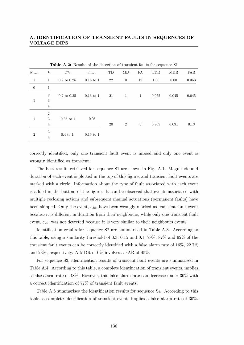
A. IDENTIFICATION OF TRANSIENT FAULTS IN SEQUENCES OFVOLTAGE DIPS
Table A.2: Results of the detection of transient faults for sequence S1
Nmax k Th tmax TD MD FA TDR MDR FAR
1 1 0.2 to 0.25 0.16 to 1 22 0 12 1.00 0.00 0.353
0 1
0.2 to 0.25 0.16 to 1 21 1 1 0.955 0.045 0.045
1
2
3
4
1
2
0.35 to 1 0.06
20 2 3 0.909 0.091 0.13
3 0.06
4
23
0.4 to 1 0.16 to 14
correctly identified, only one transient fault event is missed and only one event is
wrongly identified as transient.
The best results retrieved for sequence S1 are shown in Fig. A.1. Magnitude and
duration of each event is plotted in the top of this figure, and transient fault events are
marked with a circle. Information about the type of fault associated with each event
is added in the bottom of the figure. It can be observed that events associated with
multiple reclosing actions and subsequent manual actuations (permanent faults) have
been skipped. Only the event, e38, have been wrongly marked as transient fault event
because it is different in duration from their neighbours, while only one transient fault
event, e26, was not detected because it is very similar to their neighbours events.
Identification results for sequence S2 are summarised in Table A.3. According to
this table, using a similarity threshold of 0.3, 0.15 and 0.1, 79%, 87% and 92% of the
transient fault events can be correctly identified with a false alarm rate of 16%, 22.7%
and 23%, respectively. A MDR of 0% involves a FAR of 45%.
For sequence S3, identification results of transient fault events are summarised in
Table A.4. According to this table, a complete identification of transient events, implies
a false alarm rate of 48%. However, this false alarm rate can decrease under 30% with
a correct identification of 77% of transient fault events.
Table A.5 summarises the identification results for sequence S4. According to this
table, a complete identification of transient events implies a false alarm rate of 30%.
136

A.1 Experimental results
Figure A.1: Transient fault events in the sequence S1.
Table A.3: Results of the detection of transient faults for sequence S2
Nmax k Th tmax TD MD FA TDR MDR FAR
0 1 to 20
0 to 1 39 0 33 1.000 0.000 0.4581 1 to 4
21 0 to 1
2 to 4 0
1 4 0.1 0.26 to 0.71 36 3 11 0.923 0.077 0.234
1 4 0.15 0.26 to 0.71 34 5 10 0.872 0.128 0.227
2 4 0.3 0.41 to 0.71 31 8 6 0.795 0.205 0.162
However, this false alarm rate can decrease under 12% with a correct identification over
84% of transient fault events.
Finally, Table A.6 summarises the identification results for sequence S5. The ma-
jority of events in this sequence are due to permanent faults. According to this table,
14 of 18 transient fault events (78%) can be correctly identified but this implies that
17 events are are wrongly identified (FAR=0.55) as transient. These false alarm rate
(FAR) can be reduced under 20% with a TDR over 50%.
For all sequences the best identification results are obtained using a similarity
threshold between 0.2 to 0.35. The high values of TDR in S1 to S4 show that most
137

A. IDENTIFICATION OF TRANSIENT FAULTS IN SEQUENCES OFVOLTAGE DIPS
Table A.4: Results of the detection of transient faults for sequence S3
Nmax k Th tmax TD MD FA TDR MDR FAR
2 2 0.05 0.11 79 0 73 1 0 0.480
2 4 0.05 0.11 78 1 59 0.987 0.013 0.431
1 4 0.05 0.11 74 5 48 0.937 0.063 0.393
1 3 0.1 0.11 71 8 39 0.899 0.101 0.355
1 4 0.1 0.11 70 9 36 0.89 0.11 0.34
1 2 0.25 0.11 61 18 24 0.77 0.23 0.28
1 3 0.25 0.0658 21 24 0.73 0.27 0.29
2 3 0.3 0.16 to 0.46
1 3 0.25 0.11 57 22 21 0.72 0.28 0.27
Table A.5: Results of the detection of transient faults for sequence S4
Nmax k Th tmax TD MD FA TDR MDR FAR
2
4
0.20.06
59 0 26 1 0 0.306
1 0.15 56 3 21 0.949 0.051 0.273
2
0.2
0.31 to 0.46
55 4 16 0.932 0.068 0.225
0.3 53 6 9 0.898 0.102 0.145
0.35 52 7 7 0.881 0.119 0.119
3 to 4 0.4 50 9 2 0.847 0.153 0.038
Table A.6: Results of the detection of transient faults for sequence S5
Nmax k Th tmax TD MD FA TDR MDR FAR
1 2 to 4 0 0.06 to 1 18 0 77 1.00 0.00 0.81
2 2 0.35 0.61 to 1 16 2 38 0.89 0.11 0.70
0
1 to 4 0.3 to 0.35 0.01 14 4 17 0.78 0.22 0.55
2 0.05 0.76 to 110 8 12 0.556 0.444 0.545
4 0.05 0.36 to 0.56
10.3 0.46 to 1
9 9 2 0.50 0.50 0.180.35 0.46 to 0.56
of the transient faults are identified. The identification strategy fails (MD) especially
when similar events appear in a short period of time (for example when several tran-
sient faults occur during storms). On the other hand, small values of FAR (for example
in S1, S2 and S4) show that identification strategy does discriminate well between the
138

A.1 Experimental results
events associated with transient and permanent faults. False alarms can occur, espe-
cially when the events of a permanent fault do not have similarities in their attributes.
This occurs, for example, when fault impedance values change during the fault as in
the case of tree contacts.
139


![Discovering Spatial Weighted Frequent Itemsets in … · 2020. 4. 1. · applications of WFIM include market-basket analytics [5], spectral signature analytics in astronomical databases](https://static.fdocuments.in/doc/165x107/603e3a13d2627b4a7243b247/discovering-spatial-weighted-frequent-itemsets-in-2020-4-1-applications-of.jpg)