![CoalitionalBargaininginNetworksusers.eecs.northwestern.edu/~thanh/paper/bargaining.pdf · 2011. 11. 3. · in bargaining. This generalizes the insight of Binmore et al. [1989] that](https://static.fdocuments.in/doc/165x107/60ce5ba35d30f509ba59b3e5/coalitionalbarga-thanhpaperbargainingpdf-2011-11-3-in-bargaining-this.jpg)
Discovering Diverse Mechanisms of Migration: The...
64
Discovering Diverse Mechanisms of Migration: The Mexico-U.S. Stream from 1970 to 2000 * Filiz Garip Department of Sociology Harvard University [email protected] [DRAFT – PLEASE DO NOT CITE OR QUOTE WITHOUT PERMISSION] * Direct all correspondence to Filiz Garip, Department of Sociology, Harvard University, 33 Kirkland St., Cambridge, MA 02138 ([email protected]). This research was funded by grants from the Clark and Milton Funds at Harvard University and a Junior Faculty Synergy Semester Grant from the Weatherhead Center for International Affairs. Patricia Martín-Sánchez provided excellent research assistantship. I am grateful to Lisa Berkman, George Borjas, Paul DiMaggio, Burak Eskici, Corina Graif, Rubén Hernández-León, Kenneth Hill, Jennifer Hochschild, Sandy Jencks, Gary King, Helen Marrow, Mert Sabuncu, Edward Schumacher- Matos, Mary Waters, Chris Winship and Yu Xie for helpful advice. Participants in the Migration and Immigrant Incorporation Workshop at Harvard University and the Migration Seminar at Harvard Center for Population and Development Studies have also provided useful feedback.
Transcript of Discovering Diverse Mechanisms of Migration: The...
Discovering Diverse Mechanisms of Migration:
The Mexico-U.S. Stream from 1970 to 2000*
Filiz Garip
Department of Sociology
Harvard University
[DRAFT – PLEASE DO NOT CITE OR QUOTE WITHOUT PERMISSION]
* Direct all correspondence to Filiz Garip, Department of Sociology, Harvard University, 33 Kirkland St., Cambridge, MA 02138 ([email protected]). This research was funded by grants from the Clark and Milton Funds at Harvard University and a Junior Faculty Synergy Semester Grant from the Weatherhead Center for International Affairs. Patricia Martín-Sánchez provided excellent research assistantship. I am grateful to Lisa Berkman, George Borjas, Paul DiMaggio, Burak Eskici, Corina Graif, Rubén Hernández-León, Kenneth Hill, Jennifer Hochschild, Sandy Jencks, Gary King, Helen Marrow, Mert Sabuncu, Edward Schumacher-Matos, Mary Waters, Chris Winship and Yu Xie for helpful advice. Participants in the Migration and Immigrant Incorporation Workshop at Harvard University and the Migration Seminar at Harvard Center for Population and Development Studies have also provided useful feedback.

1
Abstract Migrants to the United States are a diverse population. This diversity, captured in various
migration theories, is overlooked in empirical applications that describe a typical narrative for an
average migrant. Using the Mexican Migration Project data from about 17,000 first-time
migrants between 1970 and 2000, this study employs cluster analysis to identify four types of
migrants with distinct configurations of characteristics. Each migrant type corresponds to a
specific theoretical account, and becomes prevalent in a specific period, depending on the
economic, social and political conditions. Strikingly, each migrant type also becomes prevalent
around the period in which its corresponding theory is developed.
2
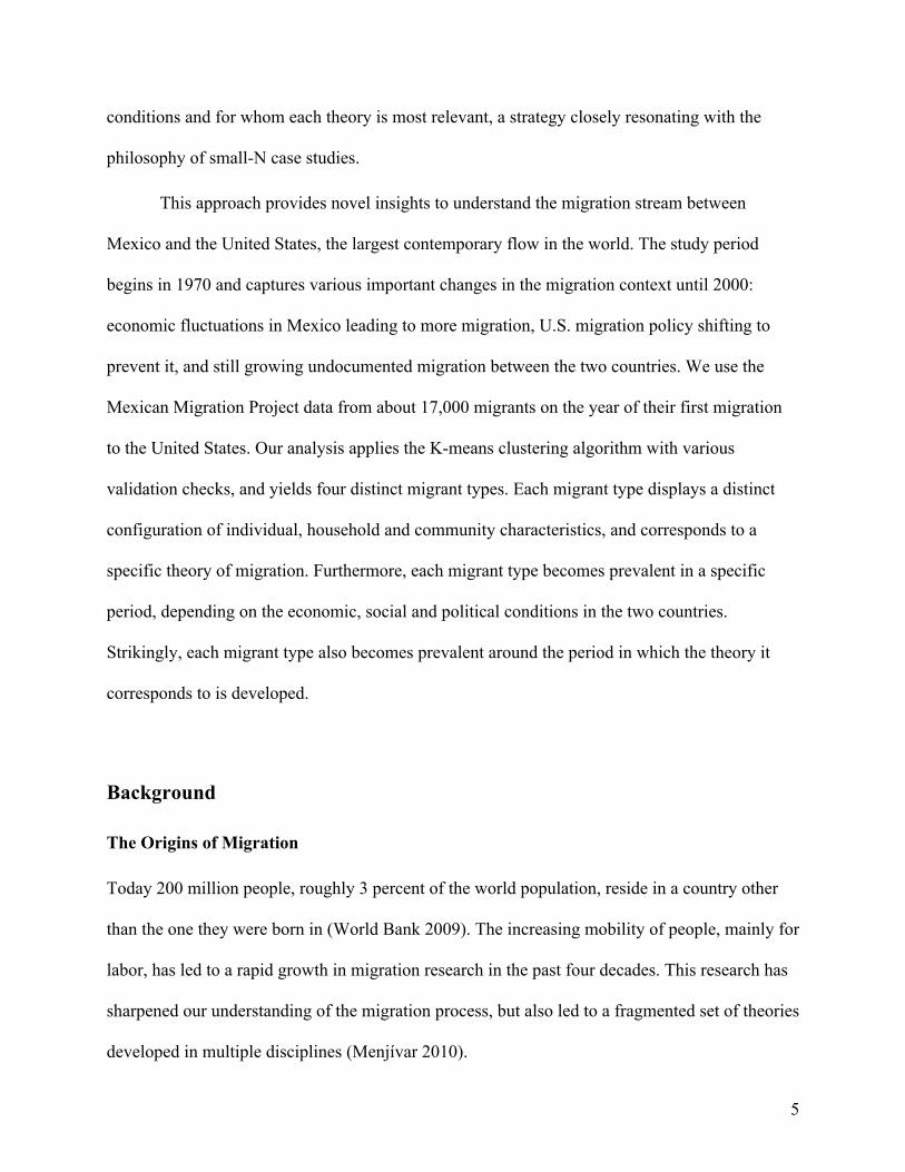
“Underneath its apparent uniformity, contemporary immigration features a bewildering variety of origins, return patterns, and modes of adaptation to American society. Never before has the United States received immigrants from so many countries, from such different social and economic backgrounds, and for so many reasons.” (Portes and Rumbaut 2006: 13)
There are diverse mechanisms that lead individuals to migrate. These mechanisms are captured
in various migration theories developed in multiple disciplines. In neo-classical economics,
higher wages in destination propel the migration of individuals who expect to earn more there
(Harris and Todaro 1970). In new economics of migration, the uncertainty in the origin economy
leads to migration from households that face risks to domestic earnings (Stark and Bloom 1985).
In cumulative causation theory, the growing web of social ties between origin and destination
fosters the migration of individuals who are connected to prior migrants (Massey 1990a).
In a seminal series of publications, Massey et al. (1993, 1994, 1998) argued that the
various causal configurations, implied by different theories, are not mutually exclusive. Income-
maximizing migrants can co-exist alongside migrants who seek to diversify risks, or those who
join family or friends in destination. Massey and Espinosa (1997) provided the first empirical
application of this argument in the Mexico-U.S. setting. Associating each theory to a set of
independent variables, the authors used regression analysis to compare which variables, and
theories, best predict who migrates. This empirical approach, although commendable in
combining various theories, did not fully reflect Massey et al.’s (1993) vision, as it treated
theories as competing, rather than complementary accounts of migration. The approach also did
not consider the conditional nature of theories, that is, the fact that each theory applies to a
specific group of individuals under specific conditions.
Indeed, in recent work, Massey and Taylor (2004: 383) critiqued their earlier work
(Massey et al. 1998) for not being able to “state with any precision which theories were most

3
important empirically in accounting for variations in the number, rate, and characteristics of
immigrants over time and whether and why different theories may prove more or less efficacious
in accounting for immigration patterns in different times and places,” and identified the major
challenge for migration research to be “test[ing] various theoretical explanations
comparatively…to determine which ones prevail under what circumstances and why.”
This study considers the challenge of characterizing the causal heterogeneity of
migration, thus takes on a major methodological problem in social science: identifying the
different mechanisms that work for different groups of individuals. Quantitative social inquiry
often focuses on (and generalizes from) an average case rather than studying the variability
across cases (Duncan 1982; Xie 2007) in an effort to emulate the natural sciences (Lieberson and
Lynn 2002). In recent years, however, new methods, such as multi-level, latent class or growth
curve models, have allowed researchers to study the variability in outcomes across different
contexts, groups or trajectories (Raudenbush and Bryk 1986; D’Unger et al. 1998; Muthén and
Muthén 2000).
Migration research has closely followed these developments. Studies have used split
samples, interaction terms or hierarchical models to show the different factors influencing
migration for men and women, among different ethnic groups, or in different contexts and time
periods (e.g., Kanaiaupuni 2000; Marcelli and Cornelius 2001; Massey, Goldring, and Durand
1994). But these studies all relied on a few fixed categories, such as gender or community, to
characterize the heterogeneity in migration, an approach that can be considered restrictive, even
essentialist (Somers 1994).
In this study, rather than dissecting or modeling data based on a few selected attributes,
we seek to discover the configurations of various attributes that characterize different migrant

4
types. This approach is inspired by Ragin and Abbott’s work in sociology. Ragin (1987) argued
that there may be multiple causal bundles that lead to the same social or historical outcome, and
these bundles may include various conditions that come together. To discover these causal
bundles, he developed Boolean algebra and fuzzy set methods (Ragin 2000). Abbot (2001)
similarly defined causes as specific configurations or sequences of events, and applied sequence
analysis, a method originally developed for classifying DNA patterns, to social data (Abbott and
Hrycak 1990).
Similar to Ragin and Abbot, we argue that different configurations of causal factors may
lead individuals to the same outcome - to migrate from Mexico to the United States. To discover
these configurations, we employ cluster analysis, an inductive and data-driven method for
locating groups of cases with similar attributes. This method allows us to identify distinct types
among migrants, thus characterize variation across cases, rather than focusing on an average
case. Hence, instead of asking “What factors determine who migrates?” we can now ask “Are
there different types of migrants in different contexts? Are these types captured in different
theories?”
Identifying configurations that characterize ‘ideal’ types has a long tradition in sociology
(Weber [1922] 1978). But, today, this tradition survives mostly in qualitative work. By using
cluster analysis to discover different migrant types, in this study, we appropriate a quantitative
method for a distinctly qualitative approach to social science. We then relate each migrant type
to a theoretical narrative, and offer an alternative way of linking evidence to theory, where
different narratives provide complementary, rather than competing, accounts of migration.
Finally, we juxtapose the temporal distribution of each migrant type against the major trends in
the economic and political context of Mexico-U.S. migration, and identify when, under what
5
conditions and for whom each theory is most relevant, a strategy closely resonating with the
philosophy of small-N case studies.
This approach provides novel insights to understand the migration stream between
Mexico and the United States, the largest contemporary flow in the world. The study period
begins in 1970 and captures various important changes in the migration context until 2000:
economic fluctuations in Mexico leading to more migration, U.S. migration policy shifting to
prevent it, and still growing undocumented migration between the two countries. We use the
Mexican Migration Project data from about 17,000 migrants on the year of their first migration
to the United States. Our analysis applies the K-means clustering algorithm with various
validation checks, and yields four distinct migrant types. Each migrant type displays a distinct
configuration of individual, household and community characteristics, and corresponds to a
specific theory of migration. Furthermore, each migrant type becomes prevalent in a specific
period, depending on the economic, social and political conditions in the two countries.
Strikingly, each migrant type also becomes prevalent around the period in which the theory it
corresponds to is developed.
Background
The Origins of Migration
Today 200 million people, roughly 3 percent of the world population, reside in a country other
than the one they were born in (World Bank 2009). The increasing mobility of people, mainly for
labor, has led to a rapid growth in migration research in the past four decades. This research has
sharpened our understanding of the migration process, but also led to a fragmented set of theories
developed in multiple disciplines (Menjívar 2010).

6
In neoclassical economics, labor migration is viewed as a product of wage and
employment differentials between regions (Harris and Todaro 1970; Sjaastad 1962). Individuals
from a low-wage origin seek to maximize their income by migrating to a high-wage destination
(Todaro 1969, 1977). The most likely migrants are individuals whose education and occupation
permit higher earnings in destination compared to the origin. These predictions have received
substantial empirical support. At the aggregate level, for example, researchers related Mexico-
U.S. migration rates to wage and employment figures in both countries (Bean et al. 1990; Frisbie
1975; Jenkins 1977; White et al. 1990). At the individual level, researchers showed that the
expected earnings in destination determined whether an individual migrates from Mexico
(Massey and Espinosa 1997; Taylor 1987), El Salvador (Funkhouser 1992), and Paraguay
(Parrado and Cerrutti 2003).
The new economics perspective views labor migration as a household act to tackle the
economic uncertainty in developing countries (Stark and Bloom 1985; Stark, Taylor, and
Yitzhaki 1986). Given insufficient markets for insurance, households send migrants as a risk
diversification strategy, where earnings in destination provide a hedge against shocks to
domestic income (Stark 1984; Stark and Levhari 1982). As a result, migrants typically originate
from households with substantial economic resources, a pattern observed in various settings
including Mexico (Massey et al. 1987), Dominican Republic (Grasmuck and Pessar 1991), and
the Philippines (Root and De Jong 1991). An alternative formulation of this theory considers
credit market failures in developing economies. In that case, households send migrants to
overcome capital constraints and to decrease their relative deprivation in the origin community
(Stark and Taylor 1989, 1991; Stark and Yitzhaki 1988). This formulation is the culmination of
earlier findings from case studies, which established migration as a strategy for supporting local

7
farm or business activities (Cornelius 1978; Roberts 1982; Wiest 1973), as well as recent results,
which showed that migrants’ earnings are often invested in the origin community (Durand et al.
1996; Lindstrom and Lauster 2001; Massey and Parrado 1994).
The neoclassical and new economics perspectives both focus on the economic conditions
that initiate labor migration. Cumulative causation theory shifts this focus to the social structure
that sustains it (Massey 1990a, 1990b). In this theory, past migration develops a growing web of
social ties between origin and destination regions. These ties increase the likelihood of future
movement by lowering the costs and increasing the benefits of migrating (Massey and García-
España 1987). The most likely migrants are individuals who have family or community ties to
prior migrants in destination. Strong evidence confirms this expectation in Mexico (Davis and
Winters 2001; Massey and Espinosa 1997; Massey and Zenteno 1999; Winters et al. 2001) and
Thailand (Curran et al. 2005; Garip 2008).1
There are two other theories that make predictions about aggregate migration flows, but
not about the specific characteristics of migrants, hence are not elaborated in this study.
Segmented labor markets theory attributes migration to the labor demand inherent in
industrialized economies (Piore 1979). Migrants fill the unskilled jobs that are undesirable to the
native workers due to low wages and status. In world systems theory, migration stems from the
1 Most studies have focused on the social ties to migrants as the principal mechanism of
cumulative causation. But, research has also identified other factors, such as the regional
distribution of human capital, the organization of agriculture or culture, that might be affected by
– and eventually affect – migration in a cumulative fashion (Massey et al. 1993). These factors
are difficult to assess reliably with the survey data at hand, and thus, are not discussed at length
here.

8
expansion of capitalist economies into developing countries (Wallerstein 1974). Migrants seek
livelihoods abroad as a response to the economic disruptions in their own countries and by
capitalizing on their increasing cultural connections to developed regions due to globalization
(Castells 1989; Sassen 1988,1991).
A Gap between Theory and Evidence
This study focuses on three theories that predict different types of migrants mobilized for
different reasons. Neoclassical economics anticipates income-maximizing migrants who expect
to earn higher wages in destination. New economics predicts risk-diversifying migrants who seek
to complement earnings at risk in origin. Cumulative causation describes network migrants who
follow family or friends in destination.
Each theory depicts a unique facet of the migration process, and combined together, they
provide a more complete picture. Considering these complementarities, Massey et al. (1993,
1994, 1998) took on a massive effort to integrate various theories of international migration.
These theories, the authors argued, carry distinct implications that need to be integrated in a
common analytic framework and evaluated empirically.
Massey and Espinosa (1997), in their comprehensive analysis of the Mexico-U.S. case,
provided the first empirical application. The authors first identified variables that captured the
predictions of various theories. The inflation rate in Mexico, for example, measured the level of
economic uncertainty, a catalyst for migration in new economics theory. The prevalence of
migration in origin community signified the density of connections to prior migrants, an
important factor leading to migration according to cumulative causation theory.
9
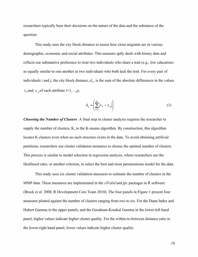
Using a regression model, and 41 such variables, the authors then evaluated which
variables better predict who migrates in 25 Mexican communities over 25 years. The variables
corresponding to the new economics and cumulative causation theories obtained substantively
meaningful and statistically significant coefficients. These theories, the authors argued, received
strong empirical support. The variables capturing neoclassical, segmented markets and world
systems perspectives had less conclusive coefficients, leading to weak support for those theories.
This empirical approach, based on regression analysis, creates a gap between theory and
evidence on migration. First, the approach juxtaposes theories against one another as competing
explanations of migration, not fully reflecting Massey et al.’s (1993) vision for these theories as
complementary accounts. Second, the approach produces average results that are presumed to
generalize to all individuals and across time. These results imply that migration theories,
conditional statements in reality, apply universally within the scope conditions of the study.
In recent years, migration scholars have made strides in addressing this issue of
population heterogeneity, that is, the fact that different mechanisms may work for specific
groups of cases. Gender scholars, for example, have shown the different reasons underlying the
migration of men and women (Cerrutti and Massey 2001; Curran and Rivero-Fuentes 2003;
Donato 1993; Hagan 1998; Hondagneu-Sotelo 1994; Kanaiaupuni 2000; Pessar 1999). Students
of assimilation have demonstrated different patterns of integration to the host society among
migrants from different ethnic groups (Alba and Nee 1997; Portes and Rumbaut 1996; Portes and
Zhou 1993). Others have studied the varying causes of migration over time or across
communities (Durand et al. 2001; Fussell and Massey 2004; Lindstrom and Lauster 2001;
Marcelli and Cornelius 2001; Massey et al. 1994).

10
This study builds on these efforts, but proposes a novel approach to characterize the
causal heterogeneity in migration. Rather than dissecting data based on a few selected attributes,
this approach employs cluster analysis to discover the distinct configurations of causal factors
that characterize different migrant types.
Migration from Mexico to the United States
Major Milestones Since 1942
This study focuses on the migration from Mexico to the United States between 1970 and 2000.
This flow, the largest in the world today gained steam with the Bracero program, which recruited
4.6 million Mexican workers to the United States for short-term farm labor from 1942 through
1964 (Cornelius 1978). The end of the Bracero program marked a shift in the U.S. immigration
policy. The changes to the Immigration and Nationality Act in 1965 and 1976 severely limited
the number of visas available to Mexicans. This condition, combined with the economic
downturn in Mexico brought on by two peso devaluations in 1976 and 1982, set off an influx of
undocumented migrants to the United States. From 1965 to 1986, about 5.7 million Mexican
migrants entered the country, 80 percent of whom were undocumented (Massey et al. 2003).
This period of mostly unhindered, undocumented migration ended with the Immigration
Reform and Control Act (IRCA) in 1986, which increased border enforcement and imposed
sanctions on employers hiring undocumented migrants. The legislation also granted amnesty to
2.3 million undocumented Mexican migrants (U.S. INS 1990). As an unintended consequence,
the amnesty created incentives for the relatives of the newly legalized Mexicans to also migrate
(Massey and Espinosa 1997). Undocumented migration to the United States continued as a result
through the 1980s, considered the ‘lost decade’ for Mexico’s economy (Sheahan 1991).

11
In 1994, two important events, the peso devaluation in Mexico and the North American
Free Trade Agreement (NAFTA) between Mexico, United States and Canada, contributed to
increasing migration flows to the United States. The former led to the worst economic crisis in
Mexico in decades, and the latter displaced rural farmers through deregulation in agriculture. As
a result, from 1994 to 1998, U.S. border apprehensions rose from 1.1 to 1.7 million (Martin
2003). By 2000, the Mexican-born persons in the United States had reached 8.4 million, of
whom 3.9 million were estimated to be undocumented (Bean et al. 2001).
Study Data
The majority of quantitative results on Mexico-U.S. migration are based on data from two
surveys: the Mexican National Survey of Population Dynamics (ENADID) and the Mexican
Migration Project (MMP).2 The former is a representative national sample, but contains
information on only labor migrants. The latter is from specific Mexican communities, but covers
all migrants, including those who have moved to the United States to join family members.
The inclusion of all migrants, not just labor-force participants, makes the MMP data more
advantageous to study the diversity of the Mexico-U.S. stream. These data are not strictly
representative of the Mexican population. Yet, prior work found that the MMP data yield an
accurate profile of the U.S. migrants in Mexico, and this profile is largely consistent with that
observed in the ENADID data (Durand et al. 2001; Zenteno and Massey 1998).
The MMP data come from 124 communities located in major migrant-sending areas in 21
Mexican states. Each community was surveyed once between 1987 and 2008, during December
2 Detailed information on the MMP is available at: http://mmp.opr.princeton.edu/.

12
and January, when the U.S. migrants are mostly likely to visit their families in Mexico. In each
community, individuals (or informants for absent individuals) from about 200 randomly selected
households were asked to provide demographic and economic information and to state the timing
of their first and last trip to the United States. Household heads were additionally asked to report
the trips in between. These data were supplemented with information from a non-random sample
of migrants identified with snowball sampling in the United States (about 10% of the sample).
Because more detailed information is available for household heads, most studies of the
MMP have restricted attention to this sub-population. To provide a more representative portrait
of migrants, this study considers all household members. The analysis seeks to identify the
diversity in the attributes of migrants on their first trip to the United States. Subsequent trips are
not considered as they are recorded only for household heads, and also to avoid a complication
that has haunted prior work on migration. This complication arises from the fact that many
attributes related to migration behavior are also changed by it. Over successive trips, migrants
gradually gain more experience, establish stronger ties to destination, and become wealthier.
Their attributes change, not as a result of the changing selectivity of the stream, but due to the
changes caused by prior migration trips. Focusing on first-time migrants allows us to observe
migrants’ attributes independently from this reciprocal relationship.
A concern with the MMP data is the retrospective nature of the information on migrants.
Let's take a household surveyed in 1990, where the daughter has migrated to the United States
for the first time in 1980. Her attributes, like age and education, were recorded in 1990, but could
be projected linearly to 1980. The economic status of her household could be reconstructed using
the data on the timing of asset purchases. The characteristics of her community could be traced
back using the retrospective community history. All these plausible steps rely on one crucial

13
assumption: that the daughter in question was living in the same household and community in
1980. While this assumption is viable for most cases, the study cannot account for the cases for
which it is not.
Methods
Cluster Analysis vs. Regression Analysis
Cluster analysis is a method for discovering groups with similar attributes in data. This method is
widely used in fields as diverse as biology, physics and computer science to produce effective
descriptions of typically large and complex data sets. Yet, in the social sciences, the method has
been overshadowed by the overwhelming popularity of regression analysis.
Regression analysis estimates parameters that characterize a relationship between an
outcome and several attributes. These parameters capture causal effects if the researcher can
credibly account for the unobserved heterogeneity in data. The causal effects, if expected
constant over time, may lead to reliable outcome predictions. Cluster analysis produces a very
different output. Rather than search for associations with an outcome, the method discovers
groups in data based on the variability in several attributes. The results, although purely
descriptive in essence, may show useful associations to outcomes of interest. For example,
different groups of migrants from Mexico may display different settlement and assimilation
patterns in the United States.
The two methods also assume different data structures. Regression methods envision a
uniform distribution of cases over the attribute space. Yet, in most social data the attributes are
correlated and the cases cluster around a few distinct configurations (Abbott 2001; Ragin 1987).

14
Regression methods can take into account these configurations by introducing interactions
between attributes. But the number of possible interactions increases exponentially with the
number of attributes and renders the model quickly unmanageable. Cluster analysis is a more
efficient method for identifying the observed configurations of attributes.
Clustering and regression methods present different approaches to learning from data.
The usefulness of either approach depends on the questions of interest, as well as the structure of
data. This study seeks to discover distinct types of migrants based on various attributes in the
MMP data. Qualitative studies suggest the presence of distinct groups among Mexico-U.S.
migrants (Portes and Rumbaut 2006), and quantitative analysis shows significant interactions
among attributes in relation to migration behavior (Curran and Rivero-Fuentes 2003). Both the
question of interest and the suspected structure of data point to cluster analysis as the method of
choice. (Other related methods include latent class and growth curve models. The former focus
on the variability in outcomes across unknown latent groups, the latter identify the variability
across trajectories. Neither is appropriate for our purpose, which is to group cases based on
configurations of causal factors (not outcomes), while keeping the outcome constant.)
Steps in Cluster Analysis
Choosing the Relevant Attributes The first step in cluster analysis is selecting the attributes for
partitioning the data. This process, similar to variable selection in regression analysis, involves
either examining the data or relying on theories to identify salient attributes. This study exploits
the vast empirical work on the MMP data, and uses several attributes that have been shown to
shape migration behavior (e.g., in Massey and Espinosa 1997).

15
The attributes, listed in Table 1, include individuals’ demographic characteristics
(whether they are household heads and/or male, years of education and occupation), household
wealth (properties, land and businesses owned), prior migration experience (whether they
migrated in Mexico, number of U.S. migrants and residents in household, and proportion of
individuals who have ever migrated in their community) and community characteristics
(proportion working in agriculture, proportion self-employed, proportion earning less than the
minimum wage and whether the community is in a metropolitan area).
[TABLE 1 ABOUT HERE]
The average values for these attributes differ significantly (p<0.05, two-tailed t-test) for
migrants and non-migrants. Migrants are individuals who have migrated at least once and non-
migrants are those who have never migrated. For the sake of comparison, both groups are
observed on the survey year in each community. (In subsequent cluster analysis, migrants are
observed on the year of their first U.S. trip.) Compared to non-migrants, migrants are more likely
to be household heads and male, to have higher levels of education, and to work in agriculture,
manufacturing or service occupations, rather than being unemployed. They live in wealthier
households with ties to U.S. migrants, and in poor and rural communities that contain a high
proportion of self-employed individuals and agricultural workers.
Similar to the evidence in prior work, the significant differences between migrants and
non-migrants observed here establish the relevance of the selected attributes for migration. Also
relevant for migration, but not included in cluster analysis, are indicators that capture important
economic or policy events, like the soaring Mexican inflation or interest rates in the 1980s or the

16
passage of IRCA in 1986. These events introduce external shocks to the migration system, and
typically shift the magnitude or composition of the migrant stream. Hence, they provide a perfect
opportunity to evaluate the migrant clusters, which, if substantively valid, should display a
temporal pattern reflecting these shifts. We explore this connection in later analyses.
The selected attributes in this study are measured on different scales. About half are
binary (e.g., gender, occupation), a few are counts (e.g., number of properties or years of
education), and the rest are continuous. Clustering methods are typically sensitive to scaling of
attributes, which determines the importance assigned to a particular attribute. To avoid an
arbitrary weighting of attributes, we dichotomize each non-binary attribute, such that the values
above the median are converted to 1 and those below it to 0.
This strategy standardizes the range of attributes, and has shown superior performance in
prior studies compared to other scaling methods that standardize the variance of attributes
(Milligan and Cooper 1988). Similar to past work, we find that the attributes standardized to the
same scale (but not the same variance) lead to the most well-separated and substantively
meaningful clustering solution in the MMP data (comparisons available upon request).3
3 In classical statistical estimation, converting continuous variables to binary attributes would
lead to a severe information loss. In cluster analysis, this approach is not only acceptable, but
used often to de-noise high variance variables (Legendre and Legendre 1983). More generally,
because the goal in statistical estimation is to estimate or confirm a given quantity (e.g., a
parameter), tuning data or methods to produce a result would lead to bias. By contrast, the goal
in cluster analysis is to create categories that reveal new information, therefore tuning data or
methods until we learn something useful is perfectly reasonable (Grimmer and King
forthcoming).

17
Choosing an Algorithm Clustering algorithms use a set of attributes to divide the data into a
given number of groups (or “clusters”) so that the cases in a group are as much alike as possible.
The output is typically a cluster membership for each case and a centroid for each cluster that
represents the “mean” (or average) of the cases in that cluster. This study employs the popular K-
means method, a classical clustering algorithm that iterates between computing K cluster
centroids by minimizing the within cluster variance and updating cluster memberships (Hastie,
Tibshirani, and Friedman 2009).
The K-means method makes no assumptions about the data structure and thus has been
generically applied to a diverse set of problems. Alternative methods typically assume a
hierarchical clustering structure or rely on a probabilistic model of the data. The former
(hierarchical) approach is useful if such a structure is substantively expected (e.g., evolutionary
trees in biology), which is not the case in this study. The latter (model-based) approach is
advantageous if the data conform to a probabilistic model, and has proven useful in low-
dimensional data sets. Yet, in our experience, the available software implementations of the
model-based approach have poor performance with large and high-dimensional data sets like the
MMP. For substantive and practical reasons, this study uses the K-means algorithm implemented
in Matlab(R) software (Matlab 2010, version 7.6). This algorithm, in addition to being generic
and fast, is in fact equivalent to the model-based approach for certain probabilistic models of the
data.
Choosing a Similarity Measure Any clustering algorithm relies on a measure of similarity, or
dissimilarity, to assess how ‘close’ cases are to one another in the attribute space. In fact,
choosing this measure is far more consequential for discovering the clustering structure in data
than specifying the algorithm itself (Hastie et al. 2009). Although there are no generic guidelines,
18
researchers typically base their decisions on the nature of the data and the substance of the
question.
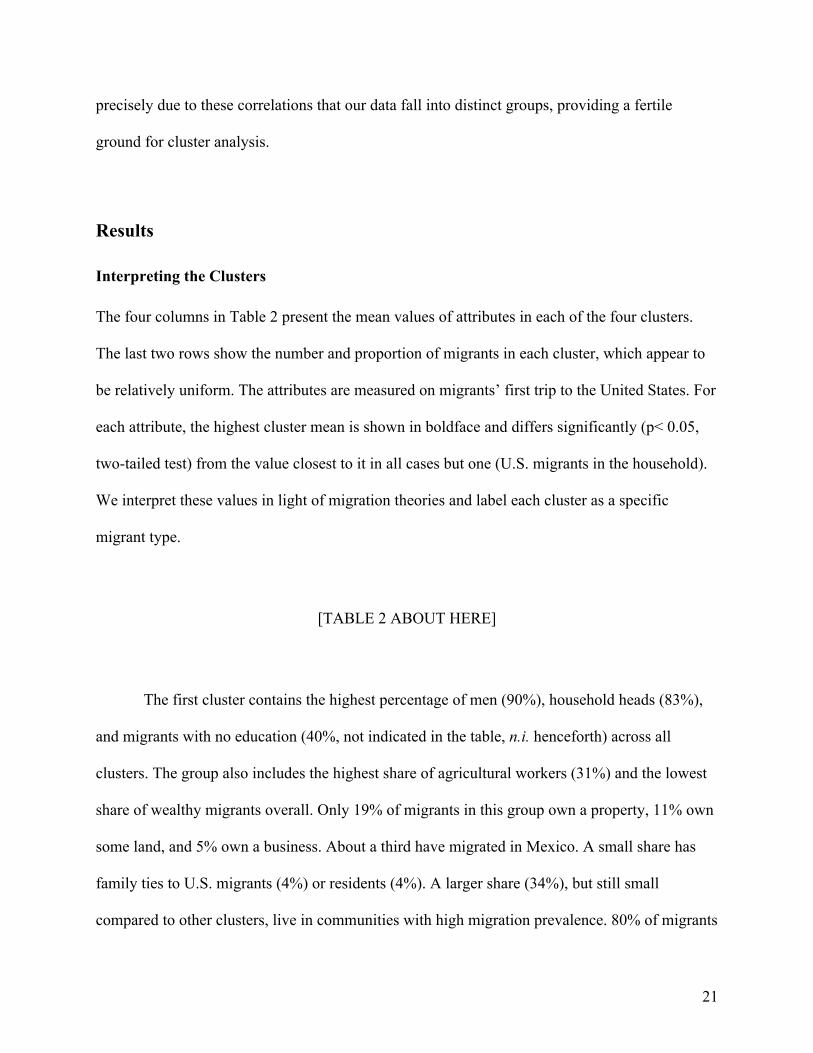
This study uses the city block distance to assess how close migrants are in various
demographic, economic and social attributes. This measure aptly deals with binary data and
reflects our substantive preference to treat two individuals who share a trait (e.g., low education)
as equally similar to one another as two individuals who both lack the trait. For every pair of
individuals i and j, the city block distance,
€
dij , is the sum of the absolute differences in the values
€
xiland
€
x jlof each attribute l=1,…,p,
€
dij = xil − x jll=1
p
∑⎛
⎝ ⎜
⎞
⎠ ⎟ (1)
Choosing the Number of Clusters A final step in cluster analysis requires the researcher to
supply the number of clusters, K, to the K-means algorithm. By construction, this algorithm
locates K clusters even when no such structure exists in the data. To avoid obtaining artificial
partitions, researchers use cluster validation measures to choose the optimal number of clusters.
This process is similar to model selection in regression analysis, where researchers use the
likelihood ratio, or another criterion, to select the best and most parsimonious model for the data.
This study uses six cluster validation measures to estimate the number of clusters in the
MMP data. These measures are implemented in the clValid and fpc packages in R software
(Brock et al. 2008; R Development Core Team 2010). The four panels in Figure 1 present four
measures plotted against the number of clusters ranging from two to six. For the Dunn Index and
Hubert Gamma in the upper panels, and the Goodman-Kruskal Gamma in the lower-left hand
panel, higher values indicate higher cluster quality. For the within-to-between distance ratio in
the lower-right hand panel, lower values indicate higher cluster quality.

19
[FIGURE 1 ABOUT HERE]
The two measures in the upper panels obtain their highest value for the 4-cluster solution.
The two measures in the lower panels reach optimal value for the 6-cluster solution, but the 4-
cluster solution is not too far off. In fact, for both measures, the 4-cluster solution corresponds to
an ‘elbow’, where the index value increases (or decreases) steeply through the 3- and 4-cluster
solutions, and only gradually thereafter.
Two additional measures, plotted against the number of clusters in Figure 2, capture the
‘stability’ of clusters to changes in the attribute space. Specifically, the average distance in the
left-hand panel, and the figure of merit in the right-hand panel, both evaluate whether the
clustering solution remains stable if attributes are removed one at a time. For both measures,
lower values indicate more stable clustering solutions. The 6-cluster solution yields the best
score in both cases, but the 4-cluster solution is also a close contender, being located at a point
where the slope of the curve changes dramatically.
[FIGURE 2 ABOUT HERE]
Based on these results, and a preference for parsimony, we choose the 4-cluster solution,
which is optimum for two measures and reasonable for the remaining four. This broad agreement
across various measures is actually rare in clustering applications and increases our confidence in
the validity of the results.

20
Assessing the Validity of Results Another useful way to assess the clustering results is to draw a
cluster heat map. Imagine each individual is represented by a vertical column of rectangles,
where each rectangle corresponds to an attribute. A gray rectangle denotes the presence of an
attribute, and a white one shows its absence. If we stack the columns for all individuals side by
side, while keeping the individuals in the same cluster together, we end up with a heat map, an
ingenious display of the entire data matrix (17 attributes x 17,049 individuals) along with the
cluster structure. Figure 3 shows the heat map for the MMP data generated by the heatplus
package in R. The rows show the attributes that are ordered so that the correlated attributes are
close to one another. The columns represent the migrant individuals. The vertical black lines
separate the four clusters.
[FIGURE 3 ABOUT HERE]
Each cluster contains migrants on their first trip to the United States, but with visibly
distinct characteristics. Migrants in cluster 1 are mostly male household heads; those in cluster 2
typically own many assets. Both groups live in poor rural communities. Migrants in cluster 3 are
mostly females and live in households or communities with former U.S. migrants. Those in
cluster 4 are relatively educated and live in urban communities.
Several attributes in the heat map are highly correlated with one another. Communities
with a high number of poor individuals also have high levels of self or agricultural employment.
Households with former U.S. migrants are typically located in communities with high levels of
migration. Individuals with a high level of education are likely to be in urban communities. It is
21
precisely due to these correlations that our data fall into distinct groups, providing a fertile
ground for cluster analysis.
Results
Interpreting the Clusters
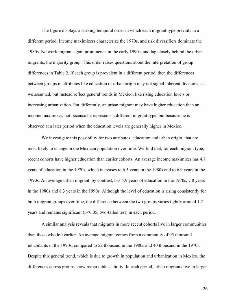
The four columns in Table 2 present the mean values of attributes in each of the four clusters.
The last two rows show the number and proportion of migrants in each cluster, which appear to
be relatively uniform. The attributes are measured on migrants’ first trip to the United States. For
each attribute, the highest cluster mean is shown in boldface and differs significantly (p< 0.05,
two-tailed test) from the value closest to it in all cases but one (U.S. migrants in the household).
We interpret these values in light of migration theories and label each cluster as a specific
migrant type.
[TABLE 2 ABOUT HERE]
The first cluster contains the highest percentage of men (90%), household heads (83%),
and migrants with no education (40%, not indicated in the table, n.i. henceforth) across all
clusters. The group also includes the highest share of agricultural workers (31%) and the lowest
share of wealthy migrants overall. Only 19% of migrants in this group own a property, 11% own
some land, and 5% own a business. About a third have migrated in Mexico. A small share has
family ties to U.S. migrants (4%) or residents (4%). A larger share (34%), but still small
compared to other clusters, live in communities with high migration prevalence. 80% of migrants

22
in this group live in rural communities with high agricultural employment, and an equal share
live in communities where a high proportion of individuals earn less than the minimum wage.
A characteristic (or an ideal-type) migrant in this cluster is a male household head who
has no education and, hence, no access to lucrative jobs in the local labor market. He lacks
income-generating assets, like land or a business, and lives in a poor rural community with
limited opportunities. Given his meager economic prospects at home, we posit that this person
migrates primarily to increase his income, and acts in line with a prediction of the neoclassical
economics. To reflect this correspondence, which we will support with circumstantial evidence
in subsequent analysis, we label this migrant, and the group he represents, as an ‘income
maximizer.’ The average income maximizer lacks the social ties to facilitate an international
move, and hence, he may migrate in Mexico first to raise the funds, or acquire the experience,
necessary for a U.S. trip.
The second cluster consists of the wealthiest migrants in the sample. 76% of these
migrants own a property, 38% own some land, and 16% own a business. Most of them have
family ties to prior U.S. migrants (80%) and live in communities with high migration prevalence
(60%). The majority are men (73%) and adult children (91%, n.i.), not heads, in the household.
40% (n.i.) of these migrants have primary education only, and about a third have some (24%) or
complete (9%) secondary education. 85% live in communities with high self employment, and a
commensurate proportion (83%) come from communities where a high proportion of individuals
earn less than the minimum wage.
A representative migrant in the second cluster is the son of the household head with only
primary education. He lives in a poor community, where the assets of his household, a property
and either a piece of land or a business, place him in the middle or upper wealth category. Given

23
his substantial economic endowments, we posit that this person migrates to diversify the risks to
those endowments in the volatile economic climate of Mexico. While the migrant, labeled a ‘risk
diversifier’ in line with the new economics theory, secures earnings in the United States, the
other members of his household, typically the head, manage the subsistence in Mexico. A risk
diversifier is expected to migrate temporarily at times of high economic uncertainty. This
expected pattern, which will be demonstrated in subsequent analysis, is probably facilitated by
the migrant’s ties to prior U.S. migrants in the family or community.
The third cluster is distinct in including mostly female migrants (62%) who are well-
connected to other migrants. 81% have family ties to U.S. migrants, 17% are connected to U.S.
residents, and 79% live in communities with high migration prevalence. Most of these migrants
are the daughter (38%, n.i.) or wife (21%, n.i.) of the household head, have primary education
only (38%, n.i.), and are unemployed (47%, n.i.). Few of them own any assets. About one in
three owns a property, one in five owns some land, and only one in ten owns a business.
Compared to the first two clusters, a lower share of them (15%) live in poor communities, but a
higher share (34%) are located in metropolitan areas.
A typical migrant in this group is the daughter of the household head who is unemployed.
At least one member of her household, probably her father or husband, is a current or prior U.S.
migrant. Given that she is not economically active, but connected to other migrants, we posit that
this person migrates to join her family members in destination and label her as a ‘network
migrant.’ Network migrants, those that follow social ties rather than economic incentives, are a
crucial component of cumulative causation theory, which predicts migration flows that are
progressively independent of the economic conditions that initiate them. We expect, and later

24
show, that network migrants become especially prevalent when family reunification policies are
in place in the United States.
The fourth cluster contains the highest percentage of educated migrants, who mostly
work in manufacturing (39%) and overwhelmingly live in urban metropolitan areas (81%). Most
of them are male (80%) and twice as likely to be the adult children (60%) rather than the heads
(31%) in their households. About one-third of these migrants have started, and about one-fifth
have finished secondary education. 67% of migrants in this cluster own a property, and 14% own
a business, the second highest share across all clusters. About a third of these migrants have
family ties to U.S. migrants, and also a third live in communities with high migration prevalence.
Only a small share of them live in communities with high agriculture (12%), or self employment
(10%), or in communities with a high share of low-wage earners (13%).
The representative migrant in this cluster is the son of the household head who has some
secondary education and lives in an urban community. Given his education and place of
residence, this migrant has access to more and better job opportunities than a typical migrant in
the other clusters. He owns a property, which provides him with economic security, but lacks
risky assets like land or business. He does not have any prior migrants in his family, and does not
live in a traditionally migrant-sending community. Based on this configuration, which is not
anticipated in any individual-level migration theory, we call this person an ‘urban migrant’ to
underline one of his most distinguishing and surprising characteristics.
In the remainder of the paper, we first evaluate the temporal patterns in the prevalence of
the four migrant types. We then consider the important economic and policy trends in the study
period in order to, first, justify the labels we have attached to the migrant types, and second, to
expose the contextual prerequisites for the emergence or dominance of those types.

25
Exploring Temporal Patterns
We identified the four migrant types based on migrants’ own, household and community
characteristics on their first trip to the United States. In this process, we included migrants
observed at different time points into a single cluster analysis and deliberately excluded
indicators for economic or policy trends that capture the Mexico-U.S. migration context. Despite
the exclusion of these trends, we still obtained results that show a strong temporal pattern.
[FIGURE 4 ABOUT HERE]
The four panels in Figure 4 show the percentage of migrants in each migrant type over
time. (We focus on percentages rather than total numbers to account for the varying sample sizes
over time.) Income maximizers, shown in the upper-left panel, comprise the majority (40%) of
migrants in the early 1970s, but decline consistently in proportion over time, and become the
minority (10%) in the 1990s. Risk diversifiers, shown in the upper-right panel, increase in
relative size through the 1970s and reach their highest level in the mid-1980s. Accounting for
almost half of all migrants then, this group shrinks relative to other groups through the 1990s,
and contains about only one-fifth of migrants in 2000. Network migrants, displayed in the lower-
left panel, show constant presence through the 1970s and 1980s, including about 15% of all
migrants. In the early 1990s, this group doubles in proportion and becomes a close second to the
majority of urban migrants. Although accounting for about a fifth of migrants in earlier years,
urban migrants increase to majority status in the early 1990s and make up about half of all
migrants in 2000.
26
The figure displays a striking temporal order in which each migrant type prevails in a
different period. Income maximizers characterize the 1970s, and risk diversifiers dominate the
1980s. Network migrants gain prominence in the early 1990s, and lag closely behind the urban
migrants, the majority group. This order raises questions about the interpretation of group
differences in Table 2. If each group is prevalent in a different period, then the differences
between groups in attributes like education or urban origin may not signal inherent divisions, as
we assumed, but instead reflect general trends in Mexico, like rising education levels or
increasing urbanization. Put differently, an urban migrant may have higher education than an
income maximizer, not because he represents a different migrant type, but because he is
observed at a later period when the education levels are generally higher in Mexico.
We investigate this possibility for two attributes, education and urban origin, that are
most likely to change in the Mexican population over time. We find that, for each migrant type,
recent cohorts have higher education than earlier cohorts. An average income maximizer has 4.7
years of education in the 1970s, which increases to 6.5 years in the 1980s and to 6.9 years in the
1990s. An average urban migrant, by contrast, has 5.9 years of education in the 1970s, 7.8 years
in the 1980s and 8.3 years in the 1990s. Although the level of education is rising consistently for
both migrant groups over time, the difference between the two groups varies tightly around 1.2
years and remains significant (p<0.05, two-tailed test) in each period.
A similar analysis reveals that migrants in more recent cohorts live in larger communities
than those who left earlier. An average migrant comes from a community of 95 thousand
inhabitants in the 1990s, compared to 52 thousand in the 1980s and 40 thousand in the 1970s.
Despite this general trend, which is due to growth in population and urbanization in Mexico, the
differences across groups show remarkable stability. In each period, urban migrants live in larger

27
communities than network migrants, who in turn live in larger communities than income
maximizers or risk diversifiers. Hence, while each migrant group displays the trends in the
general population, it still retains its distinguishing character vis-à-vis the other groups. (These
results are confirmed with regression analysis in a subsequent section.)
In the following section, we identify the contextual conditions that lead different migrants
groups to assume the majority in different periods, and hence suggest potential sources of the
temporal variation in migrant profiles.
Bringing in the Context
From 1970 to 2000, a number of economic and policy trends characterized the Mexico-U.S.
migration context. We discuss these trends chronologically below, and consider their connection
to the prevalence of different migrant types in our data. In Figure 5, we juxtapose four of these
trends against the prevalence paths for the four migrant types and detect consistent patterns of
co-variation that we describe in detail below.
Starting in the 1960s, Mexico experienced a prolonged decline in agricultural
productivity (Heath 1988; Martin 2003). This decline led to a shortage of job opportunities
(Roberts et al. 1999) and the worsening of living standards for low-income families in rural
regions (Reyes-Heroles 1983). Through the 1970s, the reductions in arable land and declining
prices of agricultural products swept the country to a deep agricultural crisis (Papail and Arroyo
2004). The increasing mechanization of agriculture in this period contributed to further
displacement of farm workers, most of whom migrated to internal or international destinations
(Arroyo 1989; Durand and Massey 1992; Yates 1981). The workers that migrated to the United

28
States filled farm jobs, which, following the Bracero program, had come to be defined as
immigrant jobs and socially unacceptable to the U.S. citizens (Massey et al. 2003; Piore 1979).
In our data, the majority of migrants in the 1970s are poor and uneducated agricultural
workers from rural communities. As the above description suggests, this group, labeled the
income maximizers, is particularly strained by the economic conditions in Mexico at the time. In
neoclassical economics theory, income maximizers are expected to migrate from a low-wage
origin to a high-wage destination to increase their earnings. This proposition implies that the
share of income maximizers in our sample should respond to changes in Mexican or U.S. wages.
[FIGURE 5 ABOUT HERE]
The upper-left panel of Figure 5 displays the percentage of income maximizers alongside
the average hourly U.S. wages over time. The values for the former series are shown in the left-
hand-side y-axis, and the values for the latter (converted to U.S.$ in year 2000) are shown in the
right-hand-side one. The two trend lines follow a similar path, and in fact are correlated at a
remarkable +0.89. Income maximizers attain their largest share, comprising 40% of the sample,
in 1970 when the U.S. wages are high, around 15$ per hour. The share of income maximizers
recedes to 30% of in 1980, when the U.S. wages have declined to 13.5$ per hour, and eventually
drops to 10% in 1990 when the U.S. wages obtain their lowest value of 12.5$ per hour. A similar
pattern ensues if we juxtapose the percentage of income maximizers against the U.S.-to-Mexico
ratio of wages (not shown). The two trend lines closely follow one another and correlate at
+0.64.

29
The close affinity between the rate of income maximizers and the U.S. wages not only
confirms the label we have assigned to this group, but also suggests that neoclassical economics
predictions hold in the Mexico-U.S. context for a specific group of individuals and under specific
economic conditions. This observation reaffirms our initial claim that migration theories are
conditional statements, and should be treated as such in empirical applications.
Along with the decline in agriculture, a number of conditions in the Mexican economy
changed in the late 1970s. In 1976, after two decades of stability, the Mexican peso was
devalued 45 percent in terms of the dollar. In the early 1980s, oil prices plummeted globally and
caused a sharp decline in Mexico’s revenues from oil exports. This decline, coinciding with two
peso devaluations in 1982, led to a significant drop in wages, and sharp increase in inflation and
interest rates (Meza 2006). These conditions hit the Mexican middle class particularly hard
(Escobar and Roberts 1991). First, the 1982 crisis caused a shift in Mexico’s development
model, and led to the state’s withdrawal from the agriculture sector and reduction of agricultural
subsidies (Alba and Potter 1986). As a result, middle-income rural families who owned small
agricultural units faced serious setbacks. Middle-income urban families, similarly, experienced
steeper wage declines than lower income families. In the city of Oaxaca, for example, families in
the top 40 percent of the income strata lost 59 percent of their income from 1977 to 1987, while
families in the bottom 60 percent lost only 14 percent (Selby 1989).
In our data, the majority of migrants in the 1980s originate from relatively wealthy
households in rural communities. These migrants, called the risk diversifiers, experience the
pronounced effect of the economic downturn and move to the United States to diversify the risks
to their subsistence. If these migrants are indeed diversifying risks, as we assumed, then the

30
timing of their move to the United States should correspond to periods of economic uncertainty
in Mexico, captured with indicators like inflation or interest rates.
The upper-right panel of Figure 5 juxtaposes the trends in the percentage of risk
diversifiers and the Mexican inflation rate. The two trend lines closely follow one another and
are strongly correlated (+0.71). Risk diversifiers attain their largest share, making up about half
of the sample, in 1985 when the Mexican inflation rate is at its highest value of 60%. As the
inflation rate drops to 10% in 1990, the share of risk diversifiers plunges to 25%. The strong
correlation between the share of risk diversifiers and the Mexican inflation rate suggests that the
predictions of the new economics theory hold particularly for this migrant group.
In addition to signaling the start of the economic recession in Mexico, the early 1980s
marked a period of political backlash against undocumented migration in the United States
which culminated in the passage of the Immigration Reform and Control Act (IRCA) in 1986
(Massey et al. 2003). IRCA, on the one hand, increased border enforcement and sanctions on
employers hiring undocumented migrants. On the other hand, it legalized 2.3 million Mexican
migrants in the United States. While the employer sanctions discouraged migration of men for
work (Bean et al. 1990), the legalizations increased migration by women and dependent children
for family reunification (Hondagneu-Sotelo 1994).
In our sample, network migrants, mostly women joining their families in the United
States, although present throughout the study period, proliferate in the years following IRCA.
These migrants, mobilized by social ties rather than economic pressures as predicted by
cumulative causation theory, become the second largest group in 1990, comprising about 30% of
all migrants, a share they maintain through the decade.

31
This pattern is observed in the lower-left panel of Figure 5, which shows side by side the
percentage of network migrants and the ratio of available visas to Mexican migrants. The two
lines both spike in the same period immediately following IRCA. Although the ratio of visas
drops after 1990, the network migrants retain their level due to higher incentives for the relatives
of the newly-legalized Mexicans to migrate as well, albeit without documents. The correlation
between the two lines is modest (+0.28) because of the pent-up demand that led to a response
that is highly skewed to the first years of the policy change, and because the ratio of visas is only
related to network migrants with documents, not to those who are undocumented.
The passage of IRCA in 1986, ironically, coincided with Mexico’s admission into
Generalized Agreement on Tariffs and Trade (GATT), which accelerated the trade flows
between Mexico and the United States at an unprecedented rate. The implementation of the
North American Free Trade Agreement (NAFTA) in 1994 further promoted the economic
integration between the two countries. The maquiladora program for example, instituted in 1965
in the border Mexican states to provide cheap labor to U.S. firms, expanded from 600 plants
employing 120,000 workers in 1980 to 4000 plants employing 1.3 million workers in 2000
(Durand et al. 2001). This expansion attracted internal migrants to the border states in Mexico
through the 1990s. Some of these internal migrants, especially indigenous Mixtecs and
Oaxacans, continued on to become international migrants to the United States (Zabin et al.
1993).
The Mexican economy, which appeared solid at the signing of NAFTA, experienced a
severe economic crisis in December 1994. Following a peso devaluation, the country defaulted
on its foreign debt, and within a year, saw its GDP shrink by 6% and its employment rate double
(Meza 2006). Around the same time, the United States was in the midst of the longest sustained

32
period of job growth in its history. The economic differentials between the two countries once
again ensured the continued flow of migrants. Different than prior years, migrants in the post-
NAFTA and post-crisis era included many educated professionals who were admitted for short-
term labor. From 1994 to 1997, the number of Mexicans admitted for temporary work (under the
H visa program) tripled and reached 37,000 persons per year (Durand et al. 2001).
In our sample, the majority of migrants in the 1990s are relatively educated, work in
manufacturing and live in urban areas. Labeled as the urban stream, the specific configuration of
this group is not anticipated in any individual-level theory of migration. A number studies,
however, have noted the increasing prevalence of migrants from urban areas in the Mexico-U.S.
stream in the late 1980s and 1990s (Roberts and Hamilton 2005; Flores, Hernández-León and
Massey 2004; Hamilton and Villarreal forthcoming), attributing this pattern to economic crises
(Cornelius 1991), increasing urbanization (Durand, Massey and Zenteno 2001), and
macroeconomic transformations prompted by foreign investments (Lozano 2001). In the most
comprehensive study to date, Hernández-León (2008) showed that the increasing numbers of
migrants from metropolitan areas can be understood within the context of the economic
restructuring in Mexico brought on by the shift in the country’s development model and the
implementation of NAFTA. These changes demolished the safety nets for skilled working-class
individuals and devalued their skill sets by transforming the industrial composition, thus
prompting them to resort to international migration as a coping strategy.
In a related line of thought, the rise of the urban stream can be explained by the
globalization arguments, which predict increasing migration flows with growing economic,
cultural and ideological linkages between countries (Sassen 1988, 1991). The educated
individuals in urban areas, the typical migrants making up the urban stream in our data, may be

33
the first to respond to these linkages. If that is the case, the proportion of the urban stream should
increase with increasing economic ties between Mexico and the United States, captured, for
instance, by the trade flows. Such a link would also validate Hernández-León’s hypothesis, as
the periods of increasing economic ties to the U.S. (e.g., due to GATT and NAFTA) overlap with
the periods of economic restructuring in Mexico.
The lower right-hand panel of Figure 5 compares the trends in the percentage of urban
migrants and the logarithm of the Mexico-U.S. trade, and provides some preliminary evidence to
this link in the MMP data. The two series, correlated at +0.77, show little movement until 1986,
when both begin to move rapidly upward. Urban migrants become the largest group in 1990 and
continually increase thereafter, mirroring the rapid uptake in the Mexico-U.S. trade. Although
this pattern suggests the plausibility of the globalization and economic restructuring hypotheses,
both of which are related to the world systems theory, more work is necessary to connect these
ideas to the specific migrant configuration we observe in the data.
The descriptive results in Figure 5 are corroborated by an OLS regression of annual
percentage of each migrant type in the overall population on all macro-economic indicators (U.S.
wages, Mexican inflation rate, visa availability and Mexico-U.S. trade). In each case, the
selected macro-economic indicator for a given group (e.g., U.S. wages for income maximizers)
has the highest effect on that group compared to the other groups, and also compared to the other
indicators for that group (which typically remain insignificant). The R2 values range from 0.22 to
0.71. (Results are available upon request.)

34
Linking Empirical Patterns to Emergence of Theories
The temporal patterns suggest that each migrant type, corresponding to a distinct theoretical
narrative, gains prevalence under specific economic, social and political conditions. Income
maximizers, representing the neoclassical narrative, are most prominent in the 1970s when the
U.S. wages are at their highest. Risk diversifiers, personifying the new economic theory, gain
majority in the 1980s when the Mexican inflation rate is at its peak. Network migrants,
symbolizing the cumulative causation theory, obtain their highest proportion in 1990s when visa
availability is at its highest. (We do not include urban migrants in the following analysis as the
specific configuration of this group is not predicted by any theoretical perspective, although its
temporal patterning seems to correspond to general trends brought on by globalization (Sassen
1988) and Mexican economic restructuring (Hernández-León 2008).)
[FIGURE 6 ABOUT HERE]
Revealing a striking pattern, the temporal order of the prevalence of the three migrant
types coincides with the temporal order of the emergence of theories on which these migrant
types are based. The three panels in Figure 6 show the proportion of income maximizers, risk
diversifiers and network migrants, respectively. The vertical lines in each panel indicate the
timing of the three most-cited articles in three theoretical perspectives: neoclassical economics,
new economics of migration and cumulative causation. 4
4 Citation data is obtained from the Social Science Citation Index (accessed in December 2009).

35
Following two initial articles by Sjaastad (1962) and Todaro (1969), Harris and Todaro
wrote the most-cited article of the neoclassical perspective in 1970 (shown in boldface in the
figure), when the income maximizers dominated the Mexico-U.S. migrant stream. Similarly,
Stark and Levhari (1982), Stark and Bloom (1985) and Stark, Taylor and Yitzaki (1986)
published the first articles launching the new economics of labor migration around the time risk
diversifiers became the majority among migrants in the MMP sample. Finally, Massey
announced the cumulative causation theory in 1990 with two simultaneous publications, closely
following his earlier work with García-España in 1987, when network migrants proliferated in
the Mexico-U.S. flows.
This overlap suggests that different migration theories depict the dominant empirical
trends in the world’s largest international migration flow around the period in which they were
developed, although they may not have been developed specifically for that purpose. In fact, the
neoclassical model of migration can be seen as an application of Mincer’s (1958) human capital
model prominent in economics at the time. Similarly, the new economics model is an extension
of the risk diversification paradigm popularized in finance by Markovitz (1959) and Sharpe
(1964). The cumulative causation theory follows from earlier work that linked social networks to
chain migration (MacDonald and MacDonald 1964). But, because these theories capture the
empirical trends of their time, even if incidentally, they are likely to be cited more than other
work.
From Descriptive Results to Testable Hypotheses
The results so far yield a useful typology of migrants with a meaningful temporal pattern that is
correlated with the trends in the economic, social and political context of Mexico-U.S. migration,
36
as well as the temporal ordering of the prominent migration theories. Since these analyses only
characterize the variation in migrants, below we raise and address three concerns that potentially
challenge our interpretations.
[TABLE 3 ABOUT HERE]
First, the characteristics that differentiate among migrant types may not be important for
differentiating between migrants and non-migrants. Put differently, these characteristics may not
have an independent effect on migration, or their effect may not vary across migrant groups as
we would expect. To investigate this point, Table 3 presents five logistic regression models of
first U.S. migration. The first model is run on a pooled sample of migrants and non-migrants
while the remaining four are run on samples containing a specific migrant group and non-
migrants. Individuals are observed annually from age 15 through the year of their first migration
(migrants) or the year of the survey (non-migrants). The models include the individual,
household and community characteristics used in the cluster analysis as well as the contextual
indicators presented in Figure 5, and correct for the multiple observations at the individual level.
(Indicators for the levels of agriculture and self-employment and the proportion earning less than
minimum wage in the community are excluded due to their high correlation (>0.70) with the
indicator for metropolitan location.)
The signs of the coefficient estimates for each migrant type are consistent with the earlier
descriptions of these types. Individuals are more likely to become an income-maximizing
migrant, for example, if they are the household head and male and if they have no education, no
properties or businesses. By contrast, individuals are more likely to become a risk-diversifying

37
migrant if they are not the household head and if they own land and properties. The estimates for
the macroeconomic indicators also present the expected patterns: the coefficient for the hourly
U.S. wages obtains its highest value for income maximizers, while the coefficient for inflation
rate is largest for risk diversifiers. Similarly, the availability of visas has its highest effect on
network migrants whereas Mexico-U.S. trade influences mostly urban migrants. Thus, the same
set of socio-demographic and economic variables has different effects on the migration
propensities in each group. Crucially, these differential effects remain hidden in the pooled
model. The counter effects of land on risk diversifiers versus urban migrants, for example, offset
one another in the pooled model, yielding an insignificant coefficient. Similarly, the differential
effects of gender or education for each group disappear in the pooled model, where the
coefficients simply reflect average effects based on the relative group sizes. These results show
that the characteristics we used for identifying different migrant types have significant effects on
migration behavior. The fact that these effects vary across groups suggests that there are diverse
mechanisms shaping the migration behavior of each group, which are bound to be obscured in
conventional pooled analyses.
To further confirm this last point, we need to address a second concern. Because each
migrant type dominates in a specific time period, the differences we observe among migrant
groups may be capturing the shifts in the population composition over time, rather than the shifts
in the mechanisms underlying migration. For example, the differences in the education levels of
urban migrants and income maximizers may be attributed to the increasing education levels in
the Mexican population, and not to an increasing importance of education for U.S. migration as
we posit. The results in Table 3 partly address this concern. The different coefficient estimates of
education for income maximizers and urban migrants suggest that these two groups do not just

38
come from different pools, but they are selected differently from these pools. (The results are
similar if we introduce year fixed-effects to control for the temporal change in migration, thus
sacrificing the identification of the macroeconomic indicators.)
To better capture the trends in population composition, we also run logistic regressions of
first U.S. migration in the pooled sample using data from sliding 3-year windows. Figure 7
shows the trends in the coefficient estimates of four key characteristics. The distribution of these
characteristics in the migrant population is likely to change over time due to the larger trends in
Mexico. For example, migrants are more likely to include women, and consequently less
household heads, in later periods due to the increasing participation of women in the labor
market. Similarly, migrants are more likely to be educated, and less likely to work in agriculture,
in later years due to the increasing levels of education and urbanization. But, because non-
migrants also experience similar changes, the shifts in the population characteristics alone should
not modify the effects of these characteristics on migration behavior over time. The results in
Figure 7 show that the effects of being a household head, male, having secondary education and
working in an agricultural occupation all change considerably over time. The effect of being
male on migration, for example, is highest in the 1970-1972 and 1982-1984 periods, but declines
from 1985 to 1991 and increases thereafter. Similarly, the effect of secondary education on
migration is negative or insignificant (depicted with white circles) prior to 1985, but increases
sharply to positive values thereafter. These patterns suggest a changing selectivity of migrants
that is independent from the changing characteristics of the population and support our
interpretation that the differences we observe among migrant groups reflect shifts in the
mechanisms and incentives underlying migration, not just shifts in population composition.

39
[FIGURE 7 ABOUT HERE]
A third concern about the results is the extent of their usefulness beyond characterizing
the heterogeneity in the sample on which they are based. Can we, for example, use the migrant
types to develop testable hypotheses? Can we then discover meaningful associations between
these types and post-migration outcomes? To answer these questions, we consider five outcomes
that characterize migrants’ experiences in the United States: (i) total number of U.S. trips, (ii)
undocumented entry, (iii) receiving residency or citizenship, (iv) being unemployed, and (v)
wages. We hypothesize that migrants will differ significantly in these outcomes based on their
cluster membership.
Given their short-term economic goals, and the lower level of border enforcement at the
time they predominantly migrate, income maximizers and risk diversifiers will make a higher
number of total U.S. trips compared to network or urban migrants. For the same reasons, these
two groups will also be more likely to cross the border without documents. Due to their
eligibility to take advantage of family reunification policies, network migrants will have a higher
likelihood of receiving U.S. residency or citizenship compared to the other three groups. This
group, however, will also be more likely to be unemployed as it comprises mostly of women and
children. Finally, urban migrants will command the highest wages of the four migrant groups
given their high levels of education and experience in manufacturing occupations.
[TABLE 4 ABOUT HERE]
40
Table 4 presents results from five models to test these hypotheses. The first and last
columns show coefficients from OLS models of the (i) logarithm of total number of U.S. trips
and (ii) logarithm of U.S. wages during first trip (in 2000 US$). The second, third and fourth
columns show odds ratios from logit models of whether the individual (i) was undocumented on
the first U.S. trip, (ii) received residency or citizenship after the first trip, and (iii) was
unemployed during the first trip. All models include year dummies. The models in the first and
third columns also include an indicator for the time elapsed from the first trip to the survey year
to control for differences among individuals in the opportunities for making U.S. trips or
obtaining legal status.
The results support all our hypotheses. Network and urban migrants make 73 (e-0.31) and
76 percent (e-0.27) percent less trips in total compared to income maximizers (model 1). These
two groups are also about 70 percent less likely to enter the U.S. without documents (model 2).
Network migrants are almost 10 times more likely to obtain legal status compared to income
maximizers (model 3), but about 7 times more likely to be unemployed during the first trip
(model 4). Finally, urban migrants earn about 10 percent more than income maximizers, their
closest follower in terms of wages.
The results show that the four migrant types differ not only in their characteristics, and
the incentives underlying their migration, but also in their experiences in the United States. The
proposed typology thus provides unique insights for extending the reach of existing theories and
for designing policies that target the discovered migrant groups to encourage certain post-
migration outcomes.

41
Conclusion
Sociology is a discipline with no dominant paradigm. Most questions can be approached from a
variety of theoretical perspectives. But in empirical applications, this diversity often gets lost. To
use prevailing quantitative methods, like regression analysis, researchers frame their questions
around average differences, for example, between persons who display a behavior and those who
do not, and reduce theories to competing sets of independent variables. If the corresponding
variables capture statistically significant differences between groups, a theory is accepted;
otherwise it is rejected. This strategy, inevitably, leads to either-or theoretical stances, rather than
an emphasis on the complementarity of varying theories.
This study proposes an alternative strategy to capture the theoretical diversity in
sociology. Instead of focusing on differences between groups who do and do not exhibit a
particular behavior, the proposed strategy calls attention to variability within a group of
individuals who display the same behavior or outcome. Are there different paths that brought
them there? Are these paths captured by different theories?
The empirical approach involves cluster analysis, a method commonly used in data-
intensive fields like biology, physics and computer science to identify subsets of cases with
similar characteristics. In this novel application to social sciences, cluster analysis discovers
distinct groups among individuals who share a behavior of interest, that is, migration. Each
group is identified by a specific configuration of characteristics and the experience of each
appears consistent with a specific theoretical account.
This approach provides a new perspective to understand the migrant stream between
Mexico and the United States. This stream, the largest in the world today, continuously increased
in the past decades leading to a migrant population of 8.4 million by 2000 (Bean et al., 2001).

42
During this period, the economic, social and political conditions in the two countries changed
drastically. These changes also shaped the character of the migrant stream, leading to a Mexican
population that is diverse in backgrounds and objectives in the United States. This diversity,
captured in a number of theories developed in economics and sociology, is overlooked in
quantitative applications that focus on describing a typical narrative for an average migrant.
Applying cluster analysis to the Mexican Migration Project (MMP) data, from about
17,000 first-time migrants over a 30-year period from 1970 to 2000, this study identified four
distinct types of migrants based on individual, household and origin community characteristics.
These types corresponded to specific theoretical accounts and gained prevalence at specific time
periods depending on the economic, social and political conditions in both countries.
Earlier migrants consisted mainly of male household heads from rural areas with little
education and few assets, who sought to increase their earnings by moving to the United States.
Labeled as income-maximizers, these migrants embodied the predictions of neoclassical
economics theory. They remained the dominant migrant type when the U.S. wages were at their
highest value in early 1970s, and slowly declined in number as the wages declined in real value.
In early 1980s, another migrant type, which we call risk-diversifiers, dominated the
Mexico-U.S. stream. These migrants came from households with substantial assets, but were not
household heads, and lived in communities where the majority of households were self-
employed. As predicted by the new economics of migration theory, they migrated to the United
States to secure earnings that insure against risks to household assets. These migrants reached
high numbers when the Mexican inflation rate, a proxy for economic uncertainty, soared from
the early to late 1980s. As the inflation rate returned back to normal in 1990s, risk-diversifiers
also declined in numbers.

43
From the mid-1980s to early 1990s, network migrants became the majority among all
first-time Mexicans migrants to the United States. These migrants, mostly women with family or
community ties to prior U.S. migrants, exemplified a prediction of cumulative causation theory:
past migration creates social ties to destination, which facilitate more migration. Network
migrants remained constant in proportion, making up about one-fifth of all migrants, until the
mid-1980s. In 1986, the Immigration and Reform Act (IRCA) legalized 2.3 million
undocumented migrants and increased the number of visas available to Mexicans. As a result,
network migrants doubled in proportion, and remained at that level until 2000.
Starting in the mid-1990s, a new migrant type quickly gained prevalence. These
migrants, which we call the urban stream, were highly educated, worked mostly in
manufacturing and lived in metropolitan areas. Constituting the majority of migrants in the
1990s, the urban stream was not predicted by any individual-level theory. Yet, a general trend of
increasing economic connectivity to the United States, and a resulting economic restructuring in
Mexico, may explain the rise of this group in our data. Given that the urban stream increased in
proportion following the increased trade between Mexico and the United States after GATT and
NAFTA, which also implied major structural changes in the Mexican economy, these hypotheses
remain plausible, but need to be evaluated in future work.
Revealing a striking pattern, each migrant type became dominant around the time in
which its corresponding theory was developed. Income-maximizing migrants prevailed in 1970s
when Harris and Todaro (1970) published the defining article of the neoclassical economics
perspective on migration. Risk-diversifiers become the majority in mid 1980s when Stark and
Bloom (1985) published the most influential article on the new economics of labor migration.
Network migrants gained prevalence in the early 1990s when Massey (1990a) developed the

44
cumulative causation theory of migration. This unanticipated finding suggests a relationship
between empirical patterns and the scientific ideas that try to capture them, and begs further
study by the sociologists of knowledge.
The empirical patterns identified in this study showed the heterogeneity in the migration
process across individuals and over time periods. The patterns suggested that different causal
regimes may govern specific groups of individuals or specific periods. These causal regimes
were scrutinized with regression analysis on sub-samples that included each migrant group and
non-migrants. The results showed that a different set of factors mobilized each group, a variation
that remained obscure in conventional regression analysis run on pooled samples. The results
thus suggested cluster analysis as a potential solution to the sample-splitting or change-point
problem in statistical analysis, concerned with identifying sub-samples for which the regression
estimates are stable. A final set of analyses demonstrated that migrant groups do not only vary in
the reasons that mobilize them, but also in their experiences in the United States, a finding that
confirmed the potential of the proposed typology for yielding testable hypotheses and extending
existing theories.
Cluster analysis provided us with a strategy to combine various theoretical perspectives
and to embrace the diversity of migrants. By searching for groups of individuals who shared the
same behavior but differed on configurations of characteristics, cluster analysis revealed the
various mechanisms that apply to each group. This approach, although quantitative in method, is
qualitative and historical in spirit. It is in solidarity with the case-oriented approach proposed by
Ragin (1987), which seeks to identify ‘constellations, configurations and conjunctures’ that
define and distinguish each case. The approach is also similar to a ‘colligation’ process, which
involves piecing together various factors to explain a case, imported from history to sociology by

45
Abbott (2001). The goal, similar to these authors’, is to close the gap between theory and
empirical evidence, and between qualitative and quantitative methods in the social sciences.
46
References
Abbott, Andrew. 2001. Time Matters: On Theory and Method. Chicago: University of Chicago Press.
Abbott, Andrew and Alexandra Hrycak. 1990. “Measuring Resemblance in Sequence Data: An Optimal Matching Analysis of Musicians’ Careers.” American Journal of Sociology 96: 144-185.
Alba, Richard and Victor Nee. 1997. “Rethinking Assimilation Theory for a New Era of Immigration.” International Migration Review 31: 826-874.
Alba, Francisco and Joseph Potter. 1986. “Population and Development in Mexico since 1940: An Interpretation.” Population and Development Review 12(1): 47-75.
Arroyo, Jesus. 1989. El abondono rural. Guadalajara, Mexico: Editorial Universidad de Guadalajara.
Bean, Frank, Rodolfo Corona, Rodolfo Tuiran, Karen Woodrow-Lafield, and Jennifer van Hook. 2001. “Circular, Invisible, and Ambiguous Migrants: Components of Difference in Estimates of the Number of Unauthorized Mexican Migrants in the United States." Demography 38: 411-422.
Bean, Frank, Thomas Espenshade, Michael White, and Robert Dymowski. 1990. “Post-IRCA Changes in the Volume and Composition of Undocumented Migration to the United States: An Assessment Based on Apprehensions Data.” In Undocumented Migration to the United States: IRCA and the Experience of the 1980s, edited by Frank Bean, Barry Edmonston, and Jeffrey Passel, pp. 111-158. Washington D.C.: The Urban Institute Press.
Brock, Guy, Vasyl Pihur, Susmita Datta, and Somnath Datta. 2008. “clValid: An R Package for Cluster Validation.” Journal of Statistical Software 25: 1-22.
Castells, Manuel. 1989. The Informational City: Information Technology, Economic Restructuring and the Urban-Regional Process. Oxford, UK: Blackwell Publishers.
Cerrutti, Marcela and Douglas Massey. 2001. “On the Auspices of Female Migration From Mexico to the United States.” Demography 38(2):187-200.
Cornelius, Wayne. 1978. Mexican Migration to the United States: Causes, Consequences, and U.S. Responses. Cambridge, MA: Center for International Studies, Massachusetts Institute of Technology.
Cornelius, Wayne. 1991. “Los migrantes de las crisis: The Changing Profile of Mexican Immigration to the United States.” In Social Responses to Mexico’s Economic Crisis of the 1980s, edited by Mercedes González de la Rocha and Augustín Escobar Latapí, pp. 155-193. San Diego: Center for U.S.-Mexican Studies, University of California, San Diego.
Curran, Sara, Filiz Garip, Chang Chung, and Kanchana Tangchonlatip. 2005. “Gendered Migrant Social Capital: Evidence from Thailand.” Social Forces 84: 225-255.
Curran, Sara and Estela Rivero-Fuentes. 2003. “Engendering Migrant Networks: The Case of Mexican Migration.” Demography 40: 289-307.
Davis, Brenda and Paul Winters. 2001. “Gender, Networks and Mexico-U.S. Migration.”
47
Journal of Development Studies 38: 1-26. Donato, Katherine. 1993. “Current Trends and Patterns of Female Migration: Evidence from
Mexico.” International Migration Review 27: 748-771. D’Unger, Amy, Kenneth Land, Patricia McCall, and Daniel Nagin. 1998. “How Many Latent
Classes of Delinquent/Criminal Careers? Results from Mixed Poisson Regression Analyses.” American Journal of Sociology 103: 1593-1630.
Durand, Jorge and Douglas Massey. 1992. “Mexican Migration to the United States: A Critical Review.” Latin American Research Review 27: 3-42.
Durand, Jorge, Douglas Massey, and Rene Zenteno. 2001. “Mexican Immigration to the United States: Continuities and Changes.” Latin American Research Review 36: 107-127.
Durand, Jorge, Emilio Parrado, and Douglas Massey. 1996. “Migradollars and Development: A Reconsideration of the Mexican Case.” International Migration Review 30: 423-444.
Escobar, Augustin and Bryan Roberts. 1991. “Urban Stratification, the Middle Classes, and Economic Change in Mexico.” In Social Responses to Mexico’s Economic Crisis of the 1980s, edited by Mercedes Gonzalez de la Rocha and Agustin Escobar, pp. 91-113. San Diego, CA: Center for US-Mexican Studies.
Everitt, Brian, Sabine Landau, and Morven Leese. 2001. Cluster Analysis. Arnold. Flores, Nadia, Rubén Hernández-León and Douglas Massey. 2004. “Social capital and
Emigration from Rural and Urban Communities.” In Crossing the Border: Research from the Mexican Migration Project, edited by Jorge Durand and Douglas Massey, pp. 184-200. New York: Russell Sage Foundation.
Frisbie, Parker. 1975. “Illegal Migration from Mexico to the United States: A Longitudinal Analysis.” International Migration Review 9: 3-13.
Funkhouser, Edward. 1992. “Mass Emigration, Remittances and Economic Adjustment: The Case of El Salvador in the 1980s.” In Immigration and the Work Force: Economic Consequences for the United States and Source Areas, edited by George Borjas and Richard Freeman, pp. 135-177. Chicago: University of Chicago Press.
Fussell, Elizabeth and Douglas Massey. 2004. “The Limits to Cumulative Causation: International Migration from Mexican Urban Areas.” Demography 41(1): 151-171.
Garip, Filiz. 2008. “Social Capital and Migration: How Do Similar Resources Lead to Divergent Outcomes?” Demography 45: 591-617.
Goodman, Leo A. 1974. “Exploratory Latent Structure Analysis Using Both Identifiable and Unidentifiable Models.” Biometrika 61: 215-231.
Grasmuck, Sherri and Patricia Pessar. 1991. Between Two Islands: Dominican International Migration. Berkeley: University of California Press.
Grimmer, Justin and Gary King. Forthcoming. “General Purpose Computer-Assisted Clustering and Conceptualization.” PNAS.
Hagan, Jacqueline. 1998. “Social Networks, Gender, and Immigrant Incorporation: Resources and Constraints.” American Sociological Review 63(1): 55-67.

48
Hamilton, Erin and Andrés Villarreal. Forthcoming. “The Geography of Mexico-U.S. Migration: Rural and Urban Differences and Spatial Dependence in the Rate of Emigration.” Social Forces.
Harris, John and Michael Todaro. 1970. “Migration, Unemployment and Development: A Two-Sector Analysis.” American Economic Review 60: 126-142.
Hastie, Trevor, Robert Tibshirani, and Jerome Friedman. 2009. The Elements of Statistical Learning: Data Mining, Inference, and Prediction. Springer, second edition.
Heath, John. 1988. “An Overview of the Mexican Agricultural Crisis.” In The Mexican Economy, edited by George Philip, pp. 129{163. London, UK: Routledge.
Hernández-León, Rubén. 2008. Metropolitan Migrants: The Migration of Urban Mexicans to the United States. Berkeley, CA: University of California Press.
Hondagneu-Sotelo, Pierrette. 1994. Gendered Transitions: Mexican Experiences of Immigration. University of California Press.
Jenkins, Craig. 1977. “Push/Pull in Recent Mexican Migration to the US.” International Migration Review 11: 178-189.
Kanaiaupuni, Shawn Malia. 2000. “Reframing the Migration Question: An Analysis of Men, Women, and Gender in Mexico.” Social Forces 78: 1311-1347.
Lazarsfeld, Paul and Neil Henry. 1968. Latent Structure Analysis. Boston, MA: Houghton Mifflin.
Legendre, Pierre and Louis Legendre. 1983. Numerical Ecology. Amsterdam: Elsevier. Lieberson, Stanley and Freda Lynn. 2002. “Barking Up the Wrong Branch: Scientific
Alternatives to the Current Model of Sociological Science.” Annual Review of Sociology 28: 1-19.
Lindstrom, David and Nathaniel Lauster. 2001. “Local Economic Opportunity and the Competing Risks of Internal and U.S. migration in Zacatecas, Mexico.” International Migration Review 35: 1232-1256.
Lozano Ascencio, Fernando. 2001. “Nuevos orígenes de la migración Mexicana a los Estados Unidos: Migrantes urbanos versus migrantes rurales.” Scripta Nova: Revista Electrónica de Geografía y Ciencas Sociales, www.ub.es/geocrit/sn-94-14.htm, accessed August 15, 2011.
MacDonald, John and Leatrice MacDonald. 1964. “Chain Migration, Ethnic Neighborhood Formation and Social Networks.” The Millbank Memorial Fund Quarterly 42(1): 82-97.
Marcelli, Enrico and Wayne Cornelius. 2001. “The Changing Profile of Mexican Migrants to the United States: New Evidence from California and Mexico.” Latin American Research Review 36: 105-131.
Markowitz, Harry. 1959. Portfolio Selection: Efficient Diversification of Investments. New Haven, CT: Yale University Press.
Martin, Philip. 2003. “Economic Integration and Migration.” Discussion Paper No. 2003/35, World Institute for Development Economics Research.
Massey, Douglas. 1990a. “Social Structure, Household Strategies, and the Cumulative Causation

49
of Migration.” Population Index 56: 3-26. Massey, Douglas. 1990b. “The Social and Economic Origins of Migration.” Annals of the
American Academy of Political and Social Science 510: 60-72.
Massey, Douglas, Rafael Alarcon, Jorge Durand, and Humberto Gonzalez. 1987. Return to Aztlan: The Social Process of International Migration from Western Mexico. Berkeley and Los Angeles: University of California Press.
Massey, Douglas, Joaquin Arango, Graeme Hugo, Ali Kouaouci, Adela Pellegrino, and Edward Taylor. 1993. “Theories of International Migration: A Review and Appraisal.” Population and Development Review 19: 431-466.
Massey, Douglas, Joaquin Arango, Graeme Hugo, Ali Kouaouci, Adela Pellegrino, and Edward Taylor. 1994. “An Evaluation of International Migration Theory: The North American Case.” Population and Development Review 20: 699-751.
Massey, Douglas, Joaquin Arango, Graeme Hugo, Ali Kouaouci, Adela Pellegrino, and Edward Taylor. 1998. Worlds in Motion: Understanding International Migration at the End of the Millenium. UK: Oxford University Press.
Massey, Douglas, Jorge Durand, and Nolan Malone. 2003. Beyond Smoke and Mirrors: Mexican Immigration in an Era of Economic Integration. New York: Russell Sage Foundation Publications.
Massey, Douglas and Kristin Espinosa. 1997. “What's Driving Mexico-U.S. Migration? A Theoretical, Empirical, and Policy Analysis.” American Journal of Sociology 102: 939-999.
Massey, Douglas and Felipe García-España. 1987. “The Social Process of International Migration.” Science 237: 733-738.
Massey, Douglas, Luin Goldring, and Jorge Durand. 1994. “Continuities in Transnational Migration: An Analysis of Nineteen Mexican Communities.” American Journal of Sociology 99: 1492-1533.
Massey, Douglas and Emilio Parrado. 1994. “Migradollars: The Remittances and Savings of Mexican Migrants to the USA.” Population Research and Policy Review13: 3-30.
Massey, Douglas and Edward Taylor. 2004. “Back to the Future: Immigration Research, Immigration Policy, and Globalization in the Twenty-First Century.” Pp. 373-88 in International Migration: Prospects and Policies in a Global Market. Oxford: Oxford University Press.
Massey, Douglas and Rene Zenteno. 1999. “The Dynamics of Mass Migration.” Proceedings of the National Academy of Sciences 96: 5328-5335.
Matlab. 2010. “Matlab 2010a: The Language of Technical Computing.” The Mathworks. Menjívar, Cecilia. 2010. “Immigrants, Immigration, and Sociology: Reflecting on the State of
the Discipline.” Sociological Inquiry 80(1): 3-27. Meza, L. González. 2006. “Transformaciones económicas en México y migración a Estados
Unidos.” In Migración México-Estados Unidos: implicaciones y retos para ambos paises, edited by A. E. Latapí, E. Z. Herrera, J. A. Alejandre and G. V. Igartúa, pp. 173-193. México, D. F., Ediciones Casa Juan Pablos.

50
Milligan, Glenn and Martha Cooper. 1988. “A Study of Standardization of Variables in Cluster Analysis.” Journal of Classification 5: 181-204.
Mincer, Jacob. 1958. “Investment in Human Capital and Personal Income Distribution.” Journal of Political Economy 46(4): 281-302.
Muthén, Bengt and Linda Muthén. 2000. “Integrating Person-Centered and Variable-Centered Analyses: Growth Mixture Modeling with Latent Trajectory Classes.” Alcoholism: Clinical and Experimental Research 24: 882-891.
Papail, Jean and Jesús Arroyo Alejandre. 2004. Los dólares de la migración. Guadalajara; Paris; Los Angeles: Universidad de Guadalajara; Institut de recherche pour le développement; Profmex; Casa Juan Pablos
Parrado, Emilio and Marcela Cerrutti. 2003. “Labor Migration between Developing Countries: The Case of Paraguay and Argentina.” International Migration Review 37: 101-132.
Pessar, Patricia. 1999. “Engendering Migration Studies: The Case of New Immigrants in the United States.” American Behavioral Scientist 42: 577-600.
Piore, Michael. 1979. Birds of Passage. Cambridge, UK: Cambridge University Press. Portes, Alejandro and Ruben G. Rumbaut. 2006. Immigrant America: A Portrait. Berkeley and
Los Angeles: University of California Press. Portes, Alejandro and Min Zhou. 1993. “The New Second Generation: Segmented Assimilation
and Its Variants.” Annals of the American Academy of Political and Social Science 530: 74-96.
R Development Core Team. 2010. “R: A Language and Environment for Statistical Computing.” ISBN 3-900051-07-0, URL http://www.R-project.org.
Ragin, Charles. 1987. The Comparative Method: Moving Beyond Qualitative and Quantitative Strategies. Berkeley and Los Angeles, CA: University of California Press.
Ragin, Charles. 2000. Fuzzy-set Social Science. Chicago: University of Chicago Press. Raudenbush, Stephen and Anthony Bryk. 1986. “A Hierarchical Model for Studying School
Effects.” Sociology of Education 59: 1-17. Reyes-Heroles, Jesus. 1983. Politica macroeconomica y nienestar en Mexico. Mexico: Fondo de
Cultura Economica. Roberts, Bryan, Reanne Frank, and Fernando Lozano-Ascencio. 1999. “Transnational Migrant
Communities and Mexican Migration to the U.S.” Ethnic and Racial Studies 22: 238-266. Roberts, Bryan and Erin Hamilton. 2007. “La nueva geografía de emigración: Zonas emergentes
de atracción y expulsión, continuidad y cambio.” In El país transnacional: Migración Mexicana y cambio social a través de la frontera, edited by Marina Ariza and Alejandro Portes. Mexico City: The Institute for Social Studies of the National Autonomous University of Mexico (UNAM).
Roberts, Kenneth. 1982. “Agrarian Structure and Labor Migration in Rural Mexico.” Population and Development Review 8: 299-322.
Root, Brenda and Gordon De Jong. 1991. “Family Migration in a Developing Country.”
51
Population Studies 45: 221-233. Sassen, Saskia. 1988. The Mobility of Labor and Capital. Cambridge, UK: Cambridge
University Press. Sassen, Saskia. 1991. The Global City: New York, London, Tokyo. Princeton, NJ: Princeton
University Press. Selby, Henry. 1989. “The Effects of the Crisis in Mexico: The Case of Oaxaca.” Texas Papers on
Mexico, no.89-05, Mexican Center, University of Texas at Austin.
Sharpe, William. 1964. “Capital Asset Prices: A Theory of Market Equilibrium under Conditions of Risk.” The Journal of Finance 19(3): 425-442.
Sheahan, John. 1991. Conflict and Change in Mexican Economic Strategy: Implications for Mexico and Latin America. La Jolla: University of California at San Diego, Center for U.S.-Mexican Studies.
Sjaastad, Larry. 1962. “The Costs and Returns of Human Migration.” Journal of Political Economy 70S: 80-93.
Somers, Margaret. 1994. “The Narrative Constitution of Identity: A Relational and Network Approach.” Theory and Society 23(5): 605-649.
Stark, Oded. 1984. “Migration Decision Making: A Review Article.” Journal of Development Economics 14: 251-259.
Stark, Oded and David Bloom. 1985. “The New Economics of Labor Migration.” American Economic Review 75: 173-178.
Stark, Oded and David Levhari. 1982. “On Migration and Risk in LDCs.” Economic Development and Cultural Change 31: 191-196.
Stark, Oded and Edward Taylor. 1989. “Relative Deprivation and International Migration.” Demography 26: 1-14.
Stark, Oded and Edward Taylor. 1991. “Migration Incentives, Migration Types: The Role of Relative Deprivation.” The Economic Journal 101: 1163-1178.
Stark, Oded, Edward Taylor and Shlomo Yitzhaki. 1986. "Remittances and Inequality." The Economic Journal 96: 722-740.
Stark, Oded and Shlomo Yitzhaki. 1988. “Labor Migration as a Response to Relative Deprivation.” Journal of Population Economics 1: 57-70.
Taylor, Edward. 1986. “Differential Migration, Networks, Information and Risk.” Research in Human Capital and Development 4: 147-171.
Taylor, Edward. 1987. “Undocumented Mexico-U.S. Migration and the Returns to Households in Rural Mexico.” American Journal of Agricultural Economics 69: 626-638.
Todaro, Michael. 1969. “A Model of Labor Migration and Urban Unemployment in Less-developed Countries.” American Economic Review 59: 138-148.
Todaro, Michael. 1977. Economic Development in the Third World. New York: Longman. U.S. INS. 1990. 1989 Statistical Yearbook of the Immigration and Naturalization Service.

52
Washington, D.C.: U.S. Government Printing Office. Wallerstein, Immanuel. 1974. The Modern World System, Capitalist Agriculture and the Origins
of the European World Economy in the Sixteenth Century. New York: Academic Press. Weber, Max. [1922] 1978. Economy and Society: An Outline of Interpretive Sociology.
Berkeley, CA: University of California Press. White, Michael, Frank Bean, and Thomas Espenshade. 1990. “The US 1986 Immigration
Reform and Control Act and Undocumented Migration to the United States.” Population Research and Policy Review 9: 93-116.
Wiest, Raymond. 1973. “Wage-Labor Migration and the Household in a Mexican Town.” Journal of Anthropological Research 29: 180-209.
Winters, Paul, Alain De Janvry, and Elizabeth Sadoulet. 2001. “Family and Community Networks in Mexico-U.S. Migration.” Journal of Human Resources 36: 159-184.
World Bank. 2009. World Development Report. Published November 6, 2008, http://go.worldbank.org/K2CBHVB7H0.
Xie, Yu. 2007. “Otis Dudley Duncan’s Legacy: The Demographic Approach to Quantitative Reasoning in Social Science.” Research in Social Stratification and Mobility 25: 141-156.
Yates, Lamartine. 1981. Mexico’s Agricultural Dilemma. Tucson, AZ: University of Arizona Press.
Zabin, Carol, Michael Kearney, David Runsten, and Anna Garcia. 1993. “A New Cycle of Poverty: Mixtec Migrants in California Agriculture.” Davis, CA: The California Institute for Rural Studies.

i
Tables
Variable Migrants Non-migrantsDemographic characteristics
Household head 0.28 0.12Male 0.72 0.45Years of education 6.86 5.97Agricultural occupation 0.20 0.07Manufacturing occupation 0.31 0.10Service occupation 0.22 0.12Unemployed 0.19 0.64
Household wealthNumber of rooms in properties 4.21 3.61Log of land value (in US$ in 2000) 3.12 2.15Number of businesses 0.41 0.37
Migration experienceMigrated in Mexico? 0.22 0.17Number of U.S. legal residents in household 0.48 0.13Number of U.S. migrants (non-residents) in household 1.81 0.72Proportion ever migrated in community 0.19 0.13
Community characteristicsProportion in agriculture in community 0.28 0.24Proportion self-employed in community 0.32 0.30Proportion earning less than min. wage in community 0.38 0.34Community in metropolitan area 0.41 0.50
N (persons) 17,049 107,838a
Table 1. Sample Characteristics for Migrants and Non-migrants in 124 Mexican Communitiesa
Migrants are individuals who have migrated at least once prior to survey year. Non-migrants are individuals who have never migrated. Means for migrants and non-migrants differ significantly (p<0.05, two-tailed test) for all variables.

ii
Variable Income Maximizers
Risk Diversifiers
Network Migrants
Urban Migrants
Demographic characteristicsHousehold head 0.83 0.02 0.07 0.32Male 0.90 0.73 0.38 0.80Some secondary education 0.17 0.24 0.24 0.30Complete secondary education 0.08 0.09 0.12 0.17Agricultural occupation 0.31 0.24 0.11 0.13Manufacturing occupation 0.31 0.29 0.23 0.39
Household wealthOwn properties 0.19 0.76 0.33 0.67Own land 0.11 0.38 0.20 0.12Own business 0.05 0.16 0.11 0.14
Migration experienceMigrated in Mexico? 0.33 0.12 0.14 0.18Any U.S. legal residents in household 0.04 0.14 0.17 0.09Any U.S. migrants (non-residents) in household 0.04 0.80 0.81 0.33Community with high migration prevalence 0.34 0.60 0.79 0.29
Community characteristicsCommunity with high agriculture employment 0.82 0.74 0.27 0.12Community with high self employment 0.69 0.85 0.27 0.10Community with high no. of low earners 0.79 0.83 0.15 0.13Community in metropolitan area 0.26 0.20 0.34 0.81
N (persons) 3,522 5,569 3,271 4,687(% of total number of migrants) 21 33 19 27
a The highest mean value for each variable is shown in boldface, and differs significantly from the value closest to it (p<0.05, two-tailed test) in all cases but one (any U.S. migrants in household).
Table 2. Migrant Characteristics by Cluster Membership in 124 Mexican Communities a

iii
!"#$%&'()*+,+)'&'+-"&*.-*+./%" 01213 44 01215 44 01213 44 01216 44 01216 447$8.")$9:,)"': 126; 44 <21= 44 0;26= 44 0123; 44 1235 44>'9" 12?5 44 @2@@ 44 @2@3 44 012<@ 44 @2;; 44A&*#'&B,":8+'-*$C 1215 44 0121< 121? 12@D 44 12@; 4E$#",."+$C:'&B,":8+'-*$C 1215 44 012@6 4 121< 12@5 44 12;@ 44F$#(9"-",."+$C:'&B,":8+'-*$C 0121= 44 012D3 44 012<5 44 12@1 12@@/%&*+89-8&'9,$++8('-*$C 123? 44 1233 44 1253 44 12?? 44 126; 44>'C8G'+-8&*C%,$++8('-*$C 125= 44 12?= 44 @21; 44 12=5 44 12=? 44E"&H*+",$&,$-)"&,$++8('-*$C 1266 44 1236 44 123= 44 12D< 44 12D6 44
7$8.")$9:,I"'9-)J8#K"&,$G,&$$#.,*C,(&$("&-*". 0121; 44 012;1 44 121D 44 012@< 44 121< 44L$%'&*-)#,$G,H'98",$G,9'C:,MNEO,*C,;111P 1211@ 01211? 121< 44 01211< 0121D 44QIC,K8.*C".. 012@6 44 0126@ 44 121@ 012@< 4 012@5 44
>*%&'-*$C,"R("&*"C+">*%&'-":,*C,>"R*+$S 12;; 44 12DD 44 126@ 4 12@3 012@5 44J8#K"&,$G,N2E2,9"%'9,&".*:"C-.,*C,)$8.")$9:, 12;? 44 12@; 12;5 44 12;= 44 12;@ 44J8#K"&,$G,N2E2,#*%&'C-.,MC$C0&".*:"C-.P,*C,)), 126; 44 12?3 44 12D3 44 12D3 44 1261 44F$##8C*-B,I*-),)*%),#*%&'-*$C,(&"H'9"C+" 126= 44 1236 44 12;= 44 @2?; 44 126@ 44
F$##8C*-B,+)'&'+-"&*.-*+.F$##8C*-B,*C,#"-&$($9*-'C,'&"' 01261 44 062<? 44 062;1 44 0123@ 44 1233 44
>'+&$"+$C$#*+,*C:*+'-$&.7$8&9B,N2E2,I'%".,MNEO,*C,;111P 12@3 44 12;3 44 1211 12@; 4 12@? 44TCG9'-*$C,&'-",U1V@W 012@@ 4 12;< 4 12<@ 44 012=6 44 012<D 44/H'*9'K*9*-B,$G,H*.'.,U1V@W 12<3 0@2;? 4 0125= 4 @23; 44 @21@ 44L$%,$G,-$-'9,>"R*+$0N2E2,-&':",MNEO,*C,;111P 12;3 44 12@D 4 012@5 44 12<= 44 12DD 44
TC-"&+"(- 0=256 44 0@;2D6 44 0<25D 44 0@;2@D 44 0@<25? 44
J,M("&.$C0B"'&.P4(X1216Y,44(X121@,M-I$0-'*9":,-".-.P2,Z".89-.,'&",9$%*-,+$"GG*+*"C-.2,E-'C:'&:,"&&$&.,'&",+$&&"+-":,G$&,+98.-"&*C%,'-,-)",*C:*H*:8'9,9"H"92,[)",.'#(9",G$&,"'+),#$:"9,*C+98:".,C$C0#*%&'C-.,M*C:*H*:8'9.,I)$,)'H",C"H"&,#*%&'-":P,'C:,-)",#*%&'C-,%&$8(,.("+*G*":,*C,-)",+$98#C,)"':*C%2,[)",&"G"&"C+",%&$8(,G$&,":8+'-*$C,*.,*C:*H*:8'9.,I*-),C$,":8+'-*$CY,-)",&"G"&"C+",%&$8(,G$&,$++8('-*$C,*.,*C:*H*:8'9.,I)$,'&",8C"#(9$B":2,TC:*+'-$&.,G$&,-)",9"H"9.,$G,'%&*+89-8&",'C:,."9G,"#(9$B#"C-,'C:,-)",(&$($&-*$C,"'&C*C%,9"..,-)'C,#*C*#8#,I'%",*C,-)",+$##8C*-B,'&","R+98:":,:8",-$,-)"*&,)*%),+$&&"9'-*$C,M\12?P,I*-),-)",*C:*+'-$&,G$&,#"-&$($9*-'C,9$+'-*$C2,
!"#$%&'(&)*+,-"+%*&./0-&"&102,*+,3&4%2/%**,05&607%$&0.&8,/*+&9(:(&6,2/"+,05&#;&<$=*+%/&6%-#%/*>,?
]B,F98.-"&,>"#K"&.)*(/99,
>*%&'C-.TC+$#",
>'R*#*^"&.Z*._,
!*H"&.*G*"&.J"-I$&_,>*%&'C-.
N&K'C,>*%&'C-.
@V<3@V565 @V;66V;D< @V;3=V;D6 @V;63VD6D @V;3=V56?

iv
Cluster membershipIncome maximizer (reference)Risk diversifier -0.15 ** 0.56 ** 7.50 ** 2.41 ** -0.06 *Network migrant -0.31 ** 0.36 ** 10.37 ** 7.90 ** -0.01Urban migrant -0.27 ** 0.32 ** 5.74 ** 2.17 ** 0.10 **
Years b/w survey and first US trip 0.002 - 1.21 ** - -Year dummies yes yes yes yes yes
N (persons) 15,969 15,895 16,025 16,026 5,381Adjusted or pseudo R2 0.15 0.03 0.18 0.08 0.09*p<0.05; **p<0.01 (two-tailed tests). Results in columns (1) and (5) are OLS coefficients; those in columns (2)-(4) are odds ratios.
Table 4. Estimates from OLS and Logistic Regression Models of Various Outcomes During or After First U.S. Migration
(1) (2) (3) (4) (5)
Log of total number of US trips
Without documents during first
US trip
Received US residency or citizenship
after first trip
Unemployed during first
US trip
Log of wages during first US trip (in 2000 US$)

v
Figures

vi

vii
Cluster 1 Cluster 2 Cluster 3 Cluster 4
Community w. high self-employ. Community w. high no. poor Community w. high agri-employ
Male
US migrants in hh Community w. high migration
Owns properties
Manuf. occup.
Some sec. educ.
Hh head
Urban community
Owns business
Sec. educ.
US residents in hh
Migrated in Mexico
Owns land
Agri. occup.
Figure 3. Heat Map of Migrant Attributes by Cluster Membership
Note: The heatmap color codes attributes (rows) of all migrants (columns). Gray indicates the presence of the attribute, and white indicates its absence. The vertical black lines separate the four clusters identified with cluster analysis.
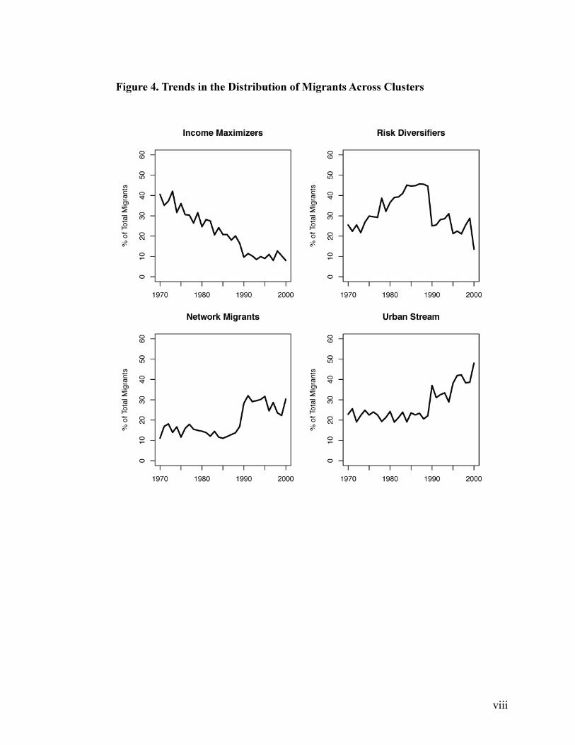
viii

ix

x

xi
!"!#
!"$#
!"%#
!"&#
!"'#
("!#
("$#
)*+,-#.*/00,./,1-#
2/34#
!"#$%&"'()!%*()
!"%#
!"5#
!"&#
!"6#
!"'#
!"7#
("!#
("(#
)*+,-#.*/00,./,1-#
2/34#
+*'%)
8!"%#
8!"$#
!"!#
!"$#
!"%#
!"&#
)*+,-#.*/00,./,1-#
2/34#
,"-%),%."/(*01)2(#.*34"/)
!"!#
!"$#
!"%#
!"&#
!"'#
("!#
("$#
)*+,-#.*/00,./,1-#
2/34#
5604.#'3#0*')7..#8*34"/)
946#0%):;)<0%/($)4/)3&%)="%>>4.4%/3)2$34-*3%$)">)9"#0)?/(4.*3"0$)4/)3&%)@""'%(),*-8'%)
9*-/:#;<,-/#.,4.=/>#,1?,.3-/#-<3-#-</#.*/00,.,/1-#,>#1*-#>,+1,0,.31-#@AB!"!5C#,1#-</#-,D/#,1-/4E3="#