Disclination Loops, Hedgehogs, and All That

Gareth P. Alexander,1, 2 Bryan Gin-ge Chen,1 Elisabetta A. Matsumoto,1, 3 and Randall D. Kamien1, ∗1Department of Physics & Astronomy, University of Pennsylvania, 209 South 33rd Street, Philadelphia PA 19104,U.S.A.2Centre for Complexity Science, Zeeman Building, University of Warwick, Coventry, CV4 7AL, U.K.3Princeton Center for Theoretical Science, Princeton University, Princeton, NJ 08544, U.S.A.

(Dated: July 7, 2011)

The homotopy theory of topological defects is a powerful tool for organizing and unifying manyideas across a broad range of physical systems. Recently, experimental progress has been madein controlling and measuring colloidal inclusions in liquid crystalline phases. The topologicalstructure of these systems is quite rich but, at the same time, subtle. Motivated by experimentand the power of topological reasoning, we review and expound upon the classification of defects inuniaxial nematic liquid crystals. Particular attention is paid to the ambiguities that arise in thesesystems, which have no counterpart in the much-storied XY model or the Heisenberg ferromagnet.

Contents

I. Introduction 1

II. Circular loops around defects: the fundamentalgroup 2A. Two-dimensional Director: RP1 2B. Making Precise Measurements 4C. Three-dimensional Director: RP2 5

III. Hedgehogs 8

IV. Disclination loops 11A. Measuring with Spheres 11B. Measuring with Tori 13

V. Biaxial nematics and the odd hedgehog 15

VI. Conclusion 17

Acknowledgments 18

References 18

I. INTRODUCTION

First identified through the beautiful textures of theirdefects, liquid crystalline materials may very well bethe ideal proving grounds for exploring notions of bro-ken symmetries, associated Goldstone modes, phenom-ena akin to the Higgs mechanism, and, of course, topo-logical defects. Indeed, the subjects of topological de-fects and liquid crystals are so intertwined that it is dif-ficult to see how a thorough understanding of one couldbe garnered without knowledge of the other. Moreover,it has proven fruitful to treat the defects as fundamen-tal excitations; solitons in the sine-Gordon model canbe treated as interacting fermions (Coleman, 1975), vor-tices in the XY model drive the Kosterlitz-Thouless phasetransition (Kosterlitz and Thouless, 1973), controlling

∗Electronic address: kamien@physics.upenn.edu

flux lines is essential for maintaining superconductivity(Nelson, 1988), and the theory of magnetic monopolesallows them to be viewed as point particles (Coleman,1988). In all of these cases, the fluctuations and configu-rations of the smooth background field around the defectscan be replaced with an effective interaction between thedefects. Thus the elasticity and statistical mechanics ofthese systems can be recast in terms of a discrete setof topological charges. Because of these successes andphysicist’s deeply-ingrained love for Gauss’s law and theconnection between flux and charge, we naturally at-tempt to interpret more complex systems in the sameterms. Unfortunately, these two cases are exceptions –in this colloquium we will emphasize this important pointand attempt to clarify if, when, and how it is appropriateto view defects as point charges.

Nematics are a prototypical liquid crystalline material– though a sample will flow like a liquid, owing to thelack of positional order, the rod-shaped, typically organicor aromatic ring molecules are locally aligned, leadingto orientational order, with widely-applied optical conse-quences. Defects in a nematic liquid crystal, as in anyordered medium, are places where the order changes dis-continuously and is thus ill-defined. They occur in theform of isolated points and lines, either system spanningwith endpoints on the boundaries of the sample or closedup into loops. We will use as our example the three-dimensional uniaxial nematic, a system that turns outnot to be as simple as it might seem. Not only is it, insome sense, the simplest counterexample to the “defectsas charges” approach, but it is also now extremely rele-vant from the experimental point of view as it has beendemonstrated that defects can be manipulated in nematiccells with great precision and variety allowing complexlinks and knots to be tied (Kamien, 2011; Tkalec, et al.,2011). Though the history or path dependence of thedefect motion at once spoils the program of reducing theconfiguration space to discrete data, it simultaneouslyintroduces a new set of topological degrees of freedomin the three-dimensional nematic. The path-dependenceimposes a non-Abelian structure to the classification of

arX

iv:1

107.

1169

v1 [

cond

-mat

.sof

t] 6

Jul

201

1

2

states. In other liquid crystalline systems, line defects inthe biaxial nematic are anticipated to entangle topolog-ically (Poenaru and Toulouse, 1977) and the interactionbetween disclinations and dislocations in smectics sufferssimilar path dependence (Chen, et al., 2009; Poenaru andToulouse, 1977). Certain non-Abelian quantum systemshave been proposed as a route to topological codes andcomputation (Kitaev, 2003; Nayak, et al., 2008).

Although they arise naturally during phase transitions,defects can also be induced deliberately by local exci-tation with a laser (Smalyukh, et al., 2009) or throughboundary conditions as with colloidal inclusions wherethe anchoring of molecules at the colloid surface inducesthe presence of defects in the surrounding liquid crys-tal. This is an especially rich technique allowing for thegeneration of a wide range of defects and for studyingthe interactions between them. For instance, the defectaccompanying a colloid may take the form of an isolatedpoint (Poulin, et al., 1997) or of a disclination loop encir-cling the particle in a ‘Saturn ring’ configuration (Teren-tjev, 1995), while two or more colloids in close proximitycan form a variety of ‘entangled’ structures where a singledisclination loop wraps around both of them (Guzman, etal., 2003; Ravnik, et al., 2007; Ravnik and Zumer, 2009).These last situations realize the interaction between lineand point defects that is a central aspect of this collo-quium.

In Section II we begin our tale by reviewing the classi-fication of topological defects by looking at point defectsin two-dimensional nematics, and line defects in three-dimensional nematics. In Section III we continue to pointdefects in three-dimensional nematics. With all the char-acters introduced, we proceed to discuss our main point:that there are only two types of unlinked disclinationloops. What we present is built on the classic reviewby Mermin on topological defects (Mermin, 1979) anda definitive result by Janich (Janich, 1987) which findsthe topological classes of uniaxial nematic textures on S3,the three-dimensional sphere, (equivalently, three dimen-sional space with fixed boundary conditions at infinity),with point and line defects. We will also discuss the bi-axial nematic phase and show that it affords additionalphysical insight into the analysis of uniaxial defects.

II. CIRCULAR LOOPS AROUND DEFECTS: THEFUNDAMENTAL GROUP

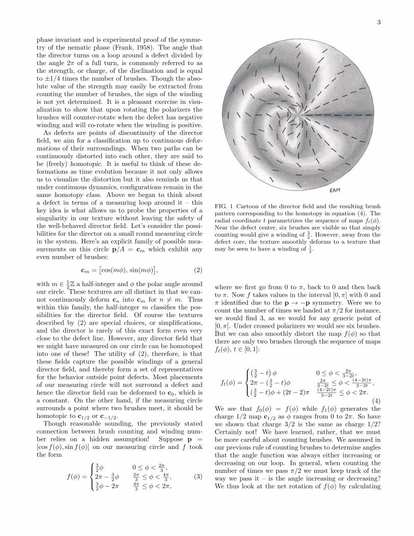
A common and distinctive experimental procedure forimaging the orientational order is to place the samplebetween crossed polarizers, yielding in nematic materialsthe characteristic Schlieren texture from which they de-rived their name. In FIG. 1 our eyes are drawn to thedark brushes and tend to follow them towards their inter-sections. The brushes typically meet at points in twos orfours; larger numbers are possible but they too are mul-tiples of two. The dark brushes correspond to regionswhere the orientation is parallel to either of the mutually

perpendicular polarizer or analyzer directions and thepoints at which they meet are disclination defects. Whydefect? Because there the orientation is ill-defined, as thebrushes would tell us to assign two or more different ori-entations to that point. We can fix this by removing thedefect point by poking a hole in the material. Physically,of course, we don’t have a hole in our sample, just a placewhere we don’t know the order. The problem is fixed byletting the magnitude of the order vanish at the origin.Then no hole is needed, but there is a point where thereis no longer nematic order and the core is in the isotropicphase. To the reader acquainted with defects in super-fluids and superconductors, this should sound familiar:in the center of an Abrikosov vortex in a superconductor(Abrikosov, 1957) the superconducting order parametervanishes and there is normal metal – a hole in the super-conductor (Chaikin and Lubensky, 1995). In all thesecases we can detect the existence of a defect without anydetailed knowledge of the disordered core: Topologicaldefects are characterized by the boundary conditions atthe interface between the higher symmetry state and thelower symmetry state. In the Schlieren texture, theseboundary conditions may be read off from the pattern ofbrushes.

In this section we introduce the basic concepts in thestudy of topological defects in this simplest case and con-nect the observation of brushes to the presence of defects.We will cover what defects are, the use of measuring sur-faces to probe them, and finally how to combine them.We begin by recalling that the continuum description ofuniaxial nematics is based upon the assignment of a lo-cal ‘average molecular orientation’ to every point in thesample, called the director field. This average orientationis that of a rod-like object, rather than an arrow, so thatthe nematic director is properly a line field, rather thana vector field. Moreover, it is only the orientation of thedirector that is important, not its magnitude, so that wemay take the director to be a unit vector n, subject tothe condition that n and −n are identified.

A. Two-dimensional Director: RP1

First we consider nematic samples in which the direc-tor always lies in the xy-plane, a prototypical thin cellsituation. Equivalently, we consider the projection of athree-dimensional director onto the xy-plane:

p = A(x, y)[cos (θ(x, y)) , sin (θ(x, y))

], (1)

where A(x, y) is the nonvanishing magnitude of the pro-jection and θ(x, y) is the angle it makes with the x-axis.Just as n and −n are identified, so too are p and −p or,equivalently, θ(x, y) and θ(x, y)+π. Because the polarizerand analyzer directions are π/2 apart, each dark brusharound a defect point tells us about a π/2 rotation ofthe director. The number of brushes counts the windingof the director field. The fact that we have defects withtwo brushes directly tells us that rotations by π leave the

3

phase invariant and is experimental proof of the symme-try of the nematic phase (Frank, 1958). The angle thatthe director turns on a loop around a defect divided bythe angle 2π of a full turn, is commonly referred to asthe strength, or charge, of the disclination and is equalto ±1/4 times the number of brushes. Though the abso-lute value of the strength may easily be extracted fromcounting the number of brushes, the sign of the windingis not yet determined. It is a pleasant exercise in visu-alization to show that upon rotating the polarizers thebrushes will counter-rotate when the defect has negativewinding and will co-rotate when the winding is positive.

As defects are points of discontinuity of the directorfield, we aim for a classification up to continuous defor-mations of their surroundings. When two paths can becontinuously distorted into each other, they are said tobe (freely) homotopic. It is useful to think of these de-formations as time evolution because it not only allowsus to visualize the distortion but it also reminds us thatunder continuous dynamics, configurations remain in thesame homotopy class. Above we began to think abouta defect in terms of a measuring loop around it – thiskey idea is what allows us to probe the properties of asingularity in our texture without leaving the safety ofthe well-behaved director field. Let’s consider the possi-bilities for the director on a small round measuring circlein the system. Here’s an explicit family of possible mea-surements on this circle p/A = cm which exhibit anyeven number of brushes:

cm =[cos(mφ), sin(mφ)

], (2)

with m ∈ 12Z a half-integer and φ the polar angle around

our circle. These textures are all distinct in that we can-not continuously deform cn into cm for n 6= m. Thuswithin this family, the half-integer m classifies the pos-sibilities for the director field. Of course the texturesdescribed by (2) are special choices, or simplifications,and the director is rarely of this exact form even veryclose to the defect line. However, any director field thatwe might have measured on our circle can be homotopedinto one of these! The utility of (2), therefore, is thatthese fields capture the possible windings of a generaldirector field, and thereby form a set of representativesfor the behavior outside point defects. Most placementsof our measuring circle will not surround a defect andhence the director field can be deformed to c0, which isa constant. On the other hand, if the measuring circlesurrounds a point where two brushes meet, it should behomotopic to c1/2 or c−1/2.

Though reasonable sounding, the previously statedconnection between brush counting and winding num-ber relies on a hidden assumption! Suppose p =[cos f(φ), sin f(φ)] on our measuring circle and f tookthe form

f(φ) =

32φ 0 ≤ φ < 2π

3 ,

2π − 32φ

2π3 ≤ φ <

4π3 ,

32φ− 2π 4π

3 ≤ φ < 2π,

(3)

FIG. 1 Cartoon of the director field and the resulting brushpattern corresponding to the homotopy in equation (4). Theradial coordinate t parametrizes the sequence of maps ft(φ).Near the defect center, six brushes are visible so that simplycounting would give a winding of 3

2. However, away from the

defect core, the texture smoothly deforms to a texture thatmay be seen to have a winding of 1

2.

where we first go from 0 to π, back to 0 and then backto π. Now f takes values in the interval [0, π] with 0 andπ identified due to the p → −p symmetry. Were we tocount the number of times we landed at π/2 for instance,we would find 3, as we would for any generic point of[0, π]. Under crossed polarizers we would see six brushes.But we can also smoothly distort the map f(φ) so thatthere are only two brushes through the sequence of mapsft(φ), t ∈ [0, 1]:

ft(φ) =

(32 − t

)φ 0 ≤ φ < 2π

3−2t ,

2π − ( 32 − t)φ

2π3−2t ≤ φ <

(4−2t)π3−2t ,

( 32 − t)φ+ (2t− 2)π (4−2t)π

3−2t ≤ φ < 2π.

(4)We see that f0(φ) = f(φ) while f1(φ) generates thecharge 1/2 map c1/2 as φ ranges from 0 to 2π. So havewe shown that charge 3/2 is the same as charge 1/2?Certainly not! We have learned, rather, that we mustbe more careful about counting brushes. We assumed inour previous rule of counting brushes to determine anglesthat the angle function was always either increasing ordecreasing on our loop. In general, when counting thenumber of times we pass π/2 we must keep track of theway we pass it – is the angle increasing or decreasing?We thus look at the net rotation of f(φ) by calculating

4

the winding number via the following integral

w =1

2π

∫ 2π

0

dφdftdφ

=1

2, (5)

for all t. In general, the winding number is precisely thecharge of the defect. In actual liquid crystal systems,energetics strongly disfavors extra brushes because thesewould correspond to regions of large splay or bend ina nematic. Thus, the naıve counting of brushes worksoutside of exceptional circumstances. Though we haveframed the discussion above in terms of a particular mea-suring circle, the classification by winding numbers holdsfor any measuring loop disjoint from the defects – justlet φ be any coordinate which goes from 0 to 2π as wetraverse the loop once. In particular, the texture on anyloop in the sample which lassos just one of the defectsis homotopic to any other; this can also be seen by thefact that the number of brushes meeting at the defect isconserved. Similarly, the number of brushes meeting at apoint in a Schlieren texture remains unchanged in time asthe texture evolves except when two defects combine andannihilate each other. The winding number m is a keyexample of an essential idea in topology: turning geomet-ric information into counting. By doing so we get robustmeasures since, in particular, integers (or half-integers),being discretely valued, cannot change continuously.

B. Making Precise Measurements

Let’s start putting our above classification into abroader context. We have mentioned several differenttopological spaces which we should keep straight. First,we are dealing with uniaxial nematic textures, so there isa space associated with the possible ground states of thedirector field, the ground state manifold (GSM)1. Here,the angle of the director Υ lives in the interval [0, π] with0 and π identified. This space is known as the real pro-jective line, RP1. Like any interval of the real line withendpoints identified, it has the topology of a circle. Next,we have the space M making up the sample volume. Forour Schlieren textures, M may be taken to be a suitableregion of the plane. Inside M there is a subspace, the setof defects Σ where the order is not defined. In the last sec-tion, Σ was the set of disclination points. We obviouslyhave the director field, an RP1-valued field on M awayfrom the defect set, n : M \ Σ→ GSM. In general, it is

1 Recall that the ground states of a nematic are just uniform tex-tures with the director pointing in some direction, so that ina general texture the local orientation can always be identifiedwith one of these ground states. Thus the changing orientationof the director in a general texture may be thought of as motionon the ground state manifold. There is not an accepted termfor this space in the literature, where it has also been called themanifold of internal states and the order parameter space.

daunting to contemplate the texture on the entire sam-ple especially if there are many defects. We also wouldlike to understand to what extent n may be understoodas arising from its behavior near the defect set – mightthere be a way to cut M \Σ into more manageable piecesaround its defects, classify those, and then glue themback together? These considerations motivate the intro-duction of auxiliary spaces: measuring surfaces of fixedtopology contained in the sample. We study the behaviorof the director field on these as we vary their placementrelative to the defect set or as we vary n. Indeed, allthe topological “charges” in this paper are defined withrespect to a choice of measuring surface. Saying that adefect carries a charge is really shorthand for saying thata small measuring surface which surrounds only that de-fect measures such a charge. If such a measuring surfaceis not present, then the “charge of a defect” is ill-defined.Of course, these ambiguities are nothing new and havebeen discussed before (Mermin, 1979). However, withthe interest in nematics and cholesterics with embeddedcolloids (Copar and Zumer, 2011; Lintuvuori et al., 2010;Musevic, et al., 2006), these mathematical subtleties areno longer just about precision or axiomatic rigor – theyare absolutely necessary for the proper interpretation ofdata. Above we measured the director on loops (whichare topologically circles, denoted by S1) and observedthat the winding number m was constant during defor-mations of the loop or the texture as long as no defectspass through the loop, which essentially solved our clas-sification problem for single defects in Schlieren textures.In more mathematical jargon, we saw that the set of mapsfrom S1 to RP1 up to homotopy (denoted [S1,RP1]) wasequivalent to the set of half-integers 1

2Z.

How can we go from single defects back to the full tex-ture? Let’s draw a picture of a two dimensional planewith punctures at the defects and small measuring loopsabout each puncture. Given the winding numbers at theloops, do we know the classification of the full texture?This picture is actually no different from one we mightdraw for the following situation: Consider a hypotheticalSchlieren texture that contains several nearby strength±1/2 defects. If we take a measurement around a circuitthat surrounds all the defects, what do we get? Beforewe say anything more about the local-to-global question,let us try to find an answer to this natural question: howcan the theory capture the intuitive notion that defectscan combine or split? We almost have it: we know thatmeasuring circuits around defects are in correspondencewith half-integers, and it happens to be true that any twohalf-integers can be added or subtracted. There is just atiny gap between question and answer now. For one, weneed to define a way to go from two measuring circuitsto one. The natural way to add loops is to concatenatethem by forming a longer loop by running over the firstand then running over the other. But in order to do this,the loops have to start and end at the same point in sam-ple or they cannot be connected. By the same token, thetwo textures traced out on the loops must start and end

5

at the same point in RP1! Given two arbitrary measur-ing loops, there’s no reason for the textures on them toagree at some point. On the other hand, our figure showsthat we can draw a big circle surrounding any pair. Isthere a way to go from two circles to one without havingto make arbitrary choices in the region between the cir-cles? Yes! Since we are interested only in properties thatare preserved under continuous deformations, we can de-form the texture around one defect so that the value inRP1 agrees at the common base point in the sample. Tovisualize this, consider a small disc around the defect.The homotopy proceeds radially outward by deformingthe original texture at the center of the disc to the newtexture at its outer edge.

This solution is inspired by the following geometricalfact: the space between a set of non-intersecting circles inthe plane can be continuously deformed to a set of circlesjoined at a single point, called a wedge sum, or bouquetof circles. Once we have the texture on the bouquet, theconcatenation of the loops is well-defined, and we thushave a definition of addition in our system. In the casehere, we may form addition by measuring around the loopwhich hugs the “outside” of the bouquet. By restrictingto sets of loops which pass through the same base point,our set of equivalence classes of maps from S1 to the GSMis enriched with the additional algebraic structure of agroup. Note that based homotopy is absolutely necessaryhere – continuous distortions of paths that preserve thebase point.

A quick aside on group theory is in order. Recall thata group requires a way of adding its elements: we justsaw that this is the concatenation of loops. In terms ofbrush counting, or the winding number, we need not beconcerned with the details of the rate at which we tra-verse the GSM, or whether we pass a brush in the firstor last half of the trip. We need only concern ourselveswith the order in which we put the two paths together.This addition of classes of paths defines the group addi-tion which may not be commutative but happens to bein this particular case. A group requires an identity: ina uniform nematic texture the map from a loop in thesample to the GSM is always constant, so this providesthe identity under the group addition. Finally, each maphas an inverse: because we can go around the GSM inthe opposite direction by backtracking our precise path,we also have an inverse. Together these properties ensurethat we have a group, known as the fundamental group,π1(GSM) – the set of based maps from a measuring cir-cuit S1 in the sample to the GSM which are equivalent upto based homotopy. And as the reader probably has al-ready guessed, this group for the case where GSM = RP1

is precisely the (half-)integers. A loop that goes aroundonly one defect in our hypothetical texture will intersecttwo brushes, giving a winding of ±1/2. A larger loopencircling both will yield a count of four if the defectshave the same sign, or zero if they have opposite signs.See Mermin’s review (Mermin, 1979) for a more detailedand precise discussion of these properties.

Though the choice of the base point is arbitrary, itsconstancy is essential and leads to many of the interest-ing phenomena we will discuss. The need for a base pointis precisely why standard time zones were developed fortrains. It is just a matter of having a single clock at onelocation (i.e. one measuring circuit) to determine theelapsed time at that spot. Two clocks can be used tomeasure elapsed time as long as they are synchronized –that is why we must have a base point. How are generalmaps from S1 to the GSM related to π1(GSM)? In thecase of Schlieren textures, we can relax: [S1,RP1] is sim-ply the underlying set of π1(RP1). Even here, however,we must remember that if we want a topological chargefor loops around defects that satisfies addition, we betterpin our loops on a base point!

Let’s conclude this section by sketching how what wehave done tells us how to go from local measurementsaround defects to the full texture. The problem of clas-sifying the defects on the full texture if we fix a basepoint is equivalent to that of classifying the texture onany bouquet of circles to which it may be retracted2. Foreach circle in the bouquet, we can choose any element ofπ1(RP1), so the classification for a bouquet of k circlesis by a k-tuple of half-integers. In this case it turns outthat this is also the answer if we allow the texture at thebase point to vary. The complication, as we will see inthe following, is that there can be more than one way totie together the measuring circuits. When π1(GSM) isnon-Abelian this freedom of choice leads to an ambiguityin measuring the “charge” of a defect. This is a majorpoint of this review and also emphasizes a possibly obvi-ous point: the Abelian or non-Abelian nature of defectsonly comes into play when there is more than one defect.Making measurements correctly is, as always, the key tounderstanding the physical system.

C. Three-dimensional Director: RP2

In our two-dimensional example, we insisted that thedirector never point perpendicular to the plane and itwas then possible to describe the texture in terms ofidealized configurations where the director was entirelyplanar. This situation is often an accurate descriptionof thin samples where the bounding surfaces are treatedto promote planar alignment. However, in bulk samples,the nematic director can point along any of the directionsin three dimensions with important implications for thetopology.

The defects described in this subsection still may becaptured by a measuring circle in the sample – in athree-dimensional nematic, these are line defects. By

2 It can be proved that “deformation retractions” of the sampleonto a smaller space don’t change the properties which can beprobed with the tools of homotopy (Hatcher, 2002).

6

considering a two-dimensional cross-section of a three-dimensional nematic, we can discuss measuring circlesaround line defects as circles surrounding points in theplane, as in the previous subsection. Thus the sum of themeasuring circles about two line defects corresponds tothe process of merging two parallel defect segments intoone. It is not hard to see that the constructions explainedin the last subsection have direct analogues for line de-fects probed this way, and we leave elaboration on mostof them to the reader. In later sections, we will probeline defects with other measuring surfaces.

The GSM here is a sphere with antipodal points iden-tified (as n and −n are identified in a line field). In thisinstance, the geometry is simple and we are able to seein our mind’s eye the topology of the GSM. In more gen-eral situations, it is useful to have something more sys-tematic: indeed, without a systematic approach we cannever be sure that our intuition is not fooling us. Thegeneral framework of the Landau theory of phase tran-sitions that exploits symmetries and symmetry breakingnot only provides well-known, systematic tools to ourproblem, but also emphasizes the essential aspect of topo-logical defects – a higher symmetry phase surrounded bya lower symmetry phase.

Recall that any rotation in three dimensions is an ele-ment of SO(3), and one set of coordinates on this spaceconsists of the three Euler angles. Write the rotation ma-trices as Rαβγ = NαMβNγ where the matrices Mβ andNγ are

Mβ =

cosβ 0 sinβ0 1 0

− sinβ 0 cosβ

,Nγ =

cos γ sin γ 0− sin γ cos γ 0

0 0 1

,(6)

and α, γ ∈ [0, 2π) and β ∈ [0, π]. Away from the de-fect, the director is a rotation of some fiducial direction,say z, so at each point ~x in space there are three an-gles α(~x), β(~x), and γ(~x), and n = Rαβγ z. The uniax-ial nematic state has two symmetries. First, because itis uniaxial, rotations around n leave the system invari-ant (a phase made of cylinders) and so we must identifyRαβγ with Rαβγ′ so that a rotation around the origi-nal z-axis does not change the state. Since we may aswell set γ′ = 0, we first see that we can parameterize alldirectors by only two angles and we only need considerthe subspace of SO(3) represented by Tαβ = Rαβ0. Thegroup of rotations around a single axis is called SO(2)and this subspace made by Tαβ is called SO(3)/SO(2)– elements of SO(3) which are identified with each otherby SO(2) rotations. Observe that this is a sphere, thespace of configurations of a unit vector, appropriate fora spin in a Heisenberg magnet, and α and β run overthe standard azimuthal and polar angles on the sphere,respectively. In a nematic, n and −n are further iden-tified; they are related by a rotation by π around anyaxis perpendicular to the director n. Again, we can pre-rotate the z direction by π using the diagonal matrixP = diag[1,−1,−1], an element of SO(3) with P2 = 1.

The two element group made of 1 and P is called Z2.The nematic symmetry forces us to identify the two ele-ments Tαβ and TαβP = Tα+π,π−β . The resulting spaceis SO(3)/H, where H is the group of nematic symme-tries (the isotropy subgroup) which includes both SO(2)and Z2. Again, the notation SO(3)/H indicates that weidentify two elements of SO(3), R and R′, if they differby any element of the group made of H = {Nα,PNα}for all α. Note that PNαP = N−α and so the productof two elements of H, Pm1Nα1 and Pm2Nα2 is

Pm1Nα1Pm2Nα2

= Pm1+m2Nα2+(−1)m2α1. (7)

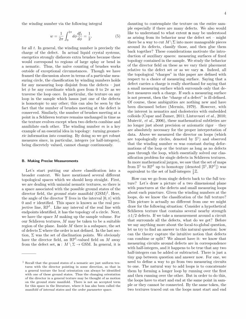
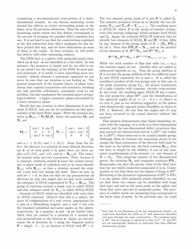
While the total number of flips just adds (m1 + m2),the rotation angles do not – whether they are added orsubtracted depends on m2. Thus the group addition inH is not just the group addition of the two different partsZ2 and SO(2) separately for m and α. H is called thesemidirect product of the two groups and, in this case, isthe point symmetry group D∞, the proper symmetriesof a right cylinder with constant, circular cross-section.In any event, the resulting space SO(3)/H has a name,the real projective plane RP2, and the identification ofthe spherical angles (θ, φ) ↔ (π − θ, φ + π) allows usto view it, just as our intuition suggested, as the spherewith diametrically opposed points identified, as shown inFIG. 2. However, the way that the angles add (7) maynot have occurred to the casual observer without thisanalysis3.

This analysis demonstrates that based measuring cir-cuits with the topology of a circle in a three-dimensionalnematic and the one-dimensional defect structures theymay encircle are characterized not by π1(RP1) but ratherby π1(RP2), which turns out to be a much smaller group.Although when we traverse our measuring circuit in thesample the final orientation of the director field must bethe same as the initial one, the final rotation Rαβγ doesnot have to simply be the identity; it can be any sym-metry transformation of the nematic, i.e. any element ofH = D∞. This subgroup consists of two disconnectedpieces, the rotations Nα and composite rotations PNα.Homotopies can alter the precise value of the final rota-tion but not which connected component it is in. Conse-quently we see that there are two classes of loops in RP2.Returning to the geometric representation of RP2 in FIG.2 as the sphere with antipodal points identified, we cansee that these two classes can be identified with loopsthat start and end at the same point on the sphere andthose that start and end at antipodal points. The pres-ence of a defect inside our measuring loop corresponds tothe latter class of paths. In the previous case, we could

3 Note that in our discussion of the two dimensional nematic, wecould have described the GSM as S1 with diameters identifiedand gone through the same construction. The resulting spaceis RP1, but its topology is identical to that of S1. S2 and RP2

are not topologically identical; in particular they have differentfundamental groups.

7

(a)

(b)

FIG. 2 The GSM for the three-dimensional nematic is the realprojective plane RP2. Any measurement around a closed loopin the sample can be mapped to a path in RP2 which belongsto one of two homotopy classes; trivial (a) and nontrivial (b).In other words, π1(RP2) = Z2.

simply count the number of brushes to determine thatπ1(RP1) = 1

2Z, the half-integers. In the case of a truethree-dimensional director we see that the group is actu-ally simpler: π1(RP2) = Z2 since any closed path on RP2

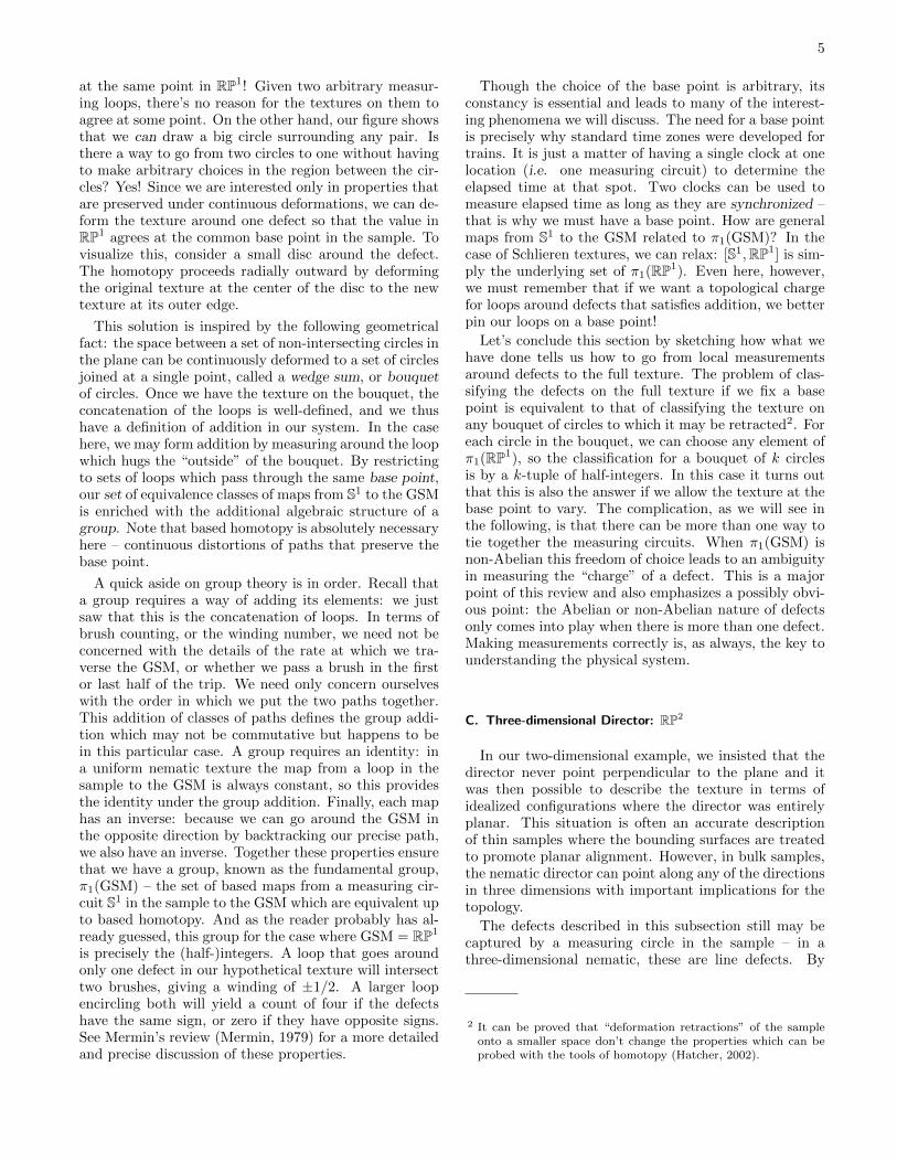
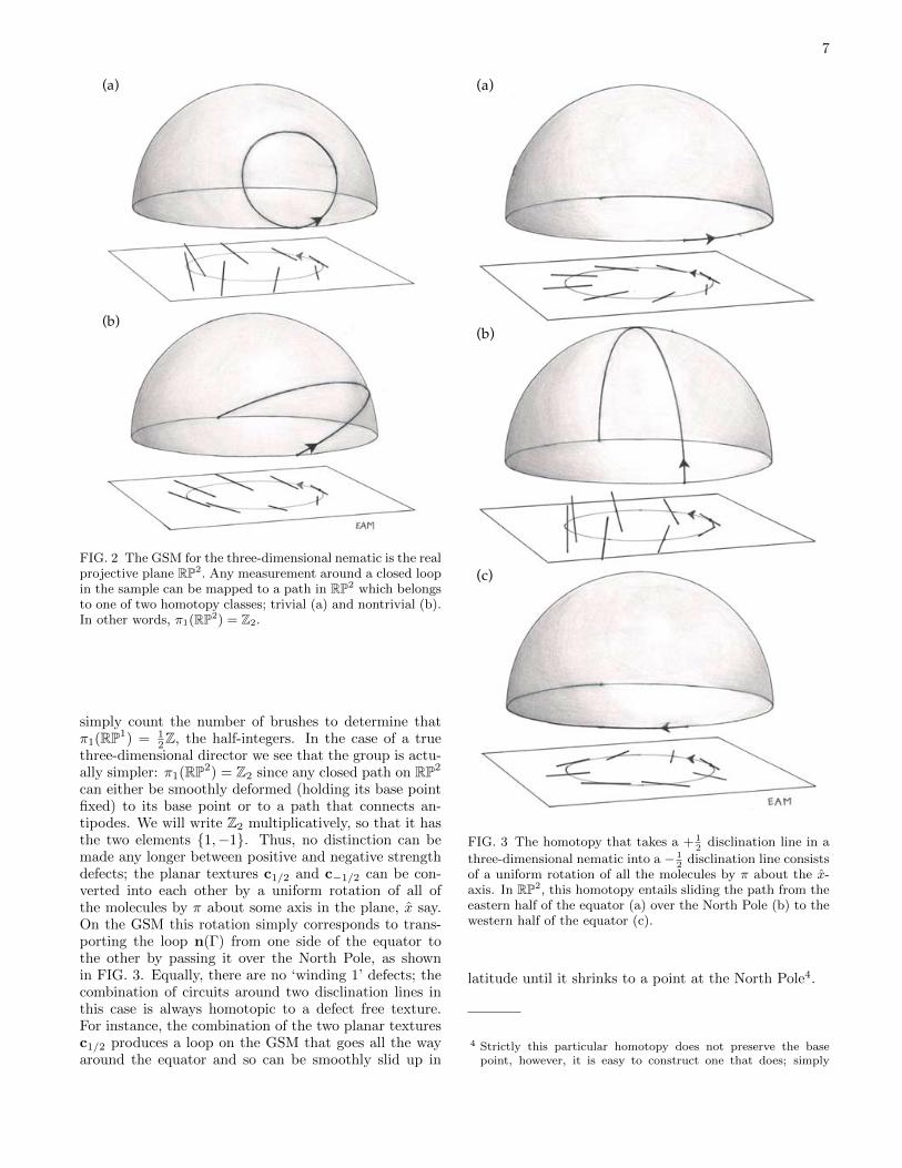
can either be smoothly deformed (holding its base pointfixed) to its base point or to a path that connects an-tipodes. We will write Z2 multiplicatively, so that it hasthe two elements {1,−1}. Thus, no distinction can bemade any longer between positive and negative strengthdefects; the planar textures c1/2 and c−1/2 can be con-verted into each other by a uniform rotation of all ofthe molecules by π about some axis in the plane, x say.On the GSM this rotation simply corresponds to trans-porting the loop n(Γ) from one side of the equator tothe other by passing it over the North Pole, as shownin FIG. 3. Equally, there are no ‘winding 1’ defects; thecombination of circuits around two disclination lines inthis case is always homotopic to a defect free texture.For instance, the combination of the two planar texturesc1/2 produces a loop on the GSM that goes all the wayaround the equator and so can be smoothly slid up in

(a)

(b)

(c)

FIG. 3 The homotopy that takes a + 12

disclination line in a

three-dimensional nematic into a − 12

disclination line consistsof a uniform rotation of all the molecules by π about the x-axis. In RP2, this homotopy entails sliding the path from theeastern half of the equator (a) over the North Pole (b) to thewestern half of the equator (c).

latitude until it shrinks to a point at the North Pole4.

4 Strictly this particular homotopy does not preserve the basepoint, however, it is easy to construct one that does; simply

8

The above homotopy from a loop covering the equa-tor to a constant loop at the North Pole is actually ob-served in cylindrical capillaries treated to give perpen-dicular anchoring at the surface. The molecules rotateout of the plane so as to align along the cylinder axis inthe interior – the so called ‘escape in the third dimen-sion’ (Cladis and Kleman, 1972; Meyer, 1973; Williamsand Bouligand, 1974). Of course, this escape can proceedin two directions: up or down. If, as typically happens,the molecules escape up in one section of the capillaryand down in another then there will be a mismatch inbetween. This gives rise to a different type of defect:point defects in three dimensions, known colloquially inthe field as hedgehogs (Polyakov, 1974).

III. HEDGEHOGS

Now that we have been introduced to the line defect,it behooves us to meet its partner, the hedgehog. Manyfeatures of the description of line defects carry over tothe point-like hedgehogs. In this paragraph, we out-line what is to come in this section by sketching a few“3-dimensional versions” of the pictures described previ-ously. First, a measuring loop can link with a defect line,but a loop cannot link with a point. Just as we need aGaussian sphere to measure a point charge in electrostat-ics, we measure the topological charge of a point defecton a measuring sphere (denoted S2) in our sample. Thuswhat we seek to classify are the set of maps without basepoint [S2,RP2] and the second homotopy group π2(RP2).With that knowledge in hand, we can consider a pieceof the sample with multiple point defects by imagininga three-dimensional ball with measuring spheres aroundpunctures at the hedgehogs. This space retracts to abouquet of spheres, and the “sum” of the textures onthe measuring spheres in the bouquet is taken to be thetexture on a sphere which shrink-wraps the entire thing.Just as for line defects, this picture relates defect additionand a local-to-global construction.

Let us first study the group structure on π2(GSM),consisting of homotopy classes of based maps from thesphere to the GSM. Here again, we fix a base point onboth the sphere (which corresponds to the base pointin our sample) and the GSM to define a group addi-tion property. To be precise, consider the standard lati-tude and longitude coordinates on the globe. We choosethe North Pole for the standard point on the sphere andsome convenient point, say Υ0, in the GSM. To com-bine elements we imagine the following sequence of ho-motopies, depicted in FIG. 4. Consider first a single ele-

hold that point of the loop fixed on the equator, slide the restover the North Pole and shrink it into the base point. In thiscase too, [S1,RP2] has the same elements as π1(RP2). In general[S1,GSM] is equal to the underlying set of the group π1(GSM)whenever the latter is Abelian.

ment g1 ∈ π2(GSM). We can smoothly deform the mapby combing out a neighborhood of the North Pole intoa polar cap which maps entirely to Υ0. We can keepsmoothly deforming the whole map into a smaller andsmaller patch of the sphere, until we have a small islandsurrounded by an ocean of points all mapping to Υ0.The texture arising on the island from a standard +1hedgehog is a skyrmion (Muhlbauer et al., 2009; Roßler,Bogdanov, and Pfleiderer, 2006) and the director rotatesfrom Υ0 at the coast all the way to the antipodal di-rection Υ0 in the interior, covering every orientation inbetween. This new map is homotopic to the original mapwhich corresponded to g1 and so, from the point of viewof π2(GSM), the new map is the same element g1 – re-member, the rate at which we traverse the GSM is not im-portant, only the places visited. We can make the samesmooth maneuver on a second element g2 ∈ π2(GSM),making a second island in the same ocean. To combinethe two elements, we simply put island one (g1) and is-land two (g2) in the same ocean without overlapping theislands. This works because the boundaries of these is-lands are all mapped to Υ0. We can now deform this newmap smoothly as we see fit, filling the ocean back up withland. In doing so we have combined the two elements.Since we can move the islands around before filling in theocean, there is no way to order the group addition andso π2(GSM) and it follows that π2 is necessarily Abelian.As in the case of π1, the identity element is again theequivalence class of the uniform texture that maps thewhole sphere to Υ0.

Finally, the inverse of any element can be found bydeforming the original map into an island and then flip-ping the island over on the sphere. Why does this givean inverse? We can connect each point on the Westernhemisphere to its reflection through the plane includingthe prime meridian in the Eastern hemisphere. We canchoose the value of the map on each of these lines in-side the two sphere to take the value at the endpoints– identical by construction. It follows that we can fillthe region inside the sphere with a smooth texture andthere can be no defects inside. Thus the island and itsmirror add to zero, shown in FIG. 5. Alternatively, wecan take the map f(θ, φ) 7→ GSM and create the inverseg(θ, φ) = f(θ,−φ).

Let’s relate the group structure of π2(GSM) to the ad-dition of defects in terms of measuring surfaces: imagine(as in FIG. 4) that we measure two different regions, eachwith a sphere. As for loops, in order to add the spheremeasurements, they must be in a bouquet configuration.We can achieve this by attaching a tubelike tether to eachsphere ending at our base point. Beware! The chargesassigned to hedgehogs (actually, assigned to measuringspheres) will depend on the choice of tethers, particu-larly if there are disclinations in the system. The sumof the textures on these spheres is equivalent to the tex-ture on a large sphere which has been deformed so thatit snugly wraps around all of the original spheres. Weencourage readers to relate this to the earlier picture of

9

(a) (b)

(c) (d)

(e)

FIG. 4 How do you combine two hedgehog charges (a)? The key lies in based homotopy theory. First, we comb the textureon the measuring surface so that the defect is confined to a small island within an ocean of uniform director field, which weidentify as the base point (b). In order to compare the relative charges of two hedgehogs, their respective measuring surfacesmust originate from the same base point, forming the bouquet of spheres described in the text (c). A new measuring surface,a sphere which has been shrink-wrapped around the bouquet of spheres, now contains both islands (d) and may be deformedinto a single sphere containing the sum of both hedgehogs (e).

islands on a single sphere – each sphere in the bouquetbecomes an island, and the base point of the bouquet isblown up to form the ocean. If no disclination lines arepresent, i.e. π1(GSM) = {1}, then the tethers can al-ways be unentangled since you “can’t lasso a basketball”(Coleman, 1988).

Though we have a definition and interpretation ofπ2(RP2), we haven’t computed it yet. In order to doso, we generalize the idea of counting brushes in the two-dimensional nematic. Each brush is a place where thedirector points in one of two directions – parallel to thepolarizer or analyzer – and the charge is one quarter thenumber of brushes. Because of the cross-polarizers, weare forced to count both the polarizer and analyzer direc-tions. However, were we given an explicit map we could,instead, just count the number of times the map fromS1 went to any single element of RP1 (with sign, as in

Eq. (5)), an integer known as the degree of the map.Then the charge of the defect would be half the degree.We could try to do the same thing for maps from S2 toRP2, but the ambiguity of n and −n makes this prob-lematic5. Each point of RP2 can be identified with twoantipodal points on S2: we can start at the base point Υ0

and choose one of the two equivalent points on S2. Givena choice, we can do this for all points in a small neigh-borhood consistently so that we locally generate a newsmooth map to S2. The only hitch might be that whentaking a long path around RP2 we may find that we are

5 The reader may worry that the same problem plagues us forπ1(RP1). It does not: RP1 is orientable where RP2 is not, whichis the real issue here.

10

FIG. 5 The inverse of an element consists of taking the mirrorimage of its island and placing this new island on the sphere.The sum of these two elements must add so that the spherecontains no defects. In the interior of the sphere, the textureis constant along chords connecting identical points on theoriginal island and its mirror. Because no defects are intro-duced, the entire texture on the sphere may now be smoothlydeformed to the base point.

hung up on a non-contractible path in the GSM when wereturn to the same point6. However, this is impossiblewith maps from S2. Fortunately, maps from S2 to anyspace X have a special property owing to the topologyof the sphere. Consider a closed loop Γ on S2 and theloop it produces on X and watch how the latter changesas we smoothly deform Γ. Because Γ can be shrunk toa point on S2, its image on X can also be shrunk to apoint and to one value in X. For the case of RP2 this isvery convenient: the image of any loop Γ on S2 must behomotopic to the identity map on RP2, so we never gethung up. Once again, we cannot lasso a basketball andso we can always “lift” the map from RP2 to S2 globallyand turn it into a map from S2 to S2. Therefore, afterfixing the lift of Υ0 (for definitiveness, we’ll take it tolie in the Northern hemisphere), π2(RP2) is the same asπ2(S2), which we can calculate.

Each map gives us a unit vector n(θ, φ) at each point ofthe measuring sphere. Like the winding number, there isan integral that measures the number of times our map

6 This is the distinction between the identity and −1 in π1(RP2):when paths in RP2 are lifted to paths in S2, paths in the equiv-alence class of the identity are closed, and paths in the class −1are not.

wraps around the sphere, also known as the degree orhedgehog charge

d =1

4π

∫S2dθdφn · [∂θn× ∂φn] . (8)

Remarkably, it is an integer: the integrand is just the Ja-cobian of the map from S2 to S2 and so it counts the areaswept out on the target sphere. Dividing by 4π simplygives us the number of times we visit each point on thetarget. Moreover, because we do not take the absolutevalue of the Jacobian, we measure positive and negativearea and thus will properly count the analog of increasingand decreasing as needed in (5) for the winding number.See, for instance, (Kamien, 2002) for the derivation ofthis Jacobian and its connection to Gaussian curvature.Therefore, we see that maps from S2 to S2 are classifiedby a degree and that this degree can be any integer, pos-itive or negative. Thus π2(RP2) = π2(S2) = Z and thereare an infinite number of topologically distinct point de-fects in nematic liquid crystals. Representatives of eachhomotopy class are given by the maps

nd(θ, φ) =[sin(θ) cos(dφ), sin(θ) sin(dφ), cos(θ)

], (9)

which exhibit a d-fold winding on the equator and maybe thought of like the textures cm of equation (2) asproviding an idealized description of the director fieldnear a hedgehog.

There remains just one point to straighten out: thequestion of the choice of lift. This will also tell us aboutthe difference between the free homotopy classes [S2,RP2]and the second homotopy group π2(RP2). Suppose wehad instead chosen to lift the base point Υ0 into theSouthern hemisphere of S2. What would be different?We would still be able to identify each element of π2(RP2)with one in π2(S2) and define a degree d through the for-mula (8). However, when we would have used the vectorn(θ, φ) to specify our texture we would now use −n(θ, φ).Since equation (8) is odd in n the degree we now mea-sure would be −d instead of d. This is not to say that thetextures labelled by d and−d are the same; the identifica-tion we made between π2(RP2) and π2(S2) is one-to-one,it’s just that there are two identifications that we canmake, differing in whether we lift the base point to theNorthern or Southern hemisphere, and these are not thesame7. So long as we make our choice of lift consistently,hedgehogs with charge d and −d are distinct, but it is upto us which sign we associate to which hedgehog8.

7 The reader might be concerned that the same ambiguity arisesfor π1(RP1). However the two choices of lift from RP1 to S1 differby a π rotation, i.e., to replacing ft(φ) with ft(φ)+π in equation(5), which does not change the winding number w. In this caseboth lifts yield the same identification of π1(RP1) with π1(S1).

8 The prevailing convention in the literature is to consider thepurely radial texture, equation (9) with d = 1, to have posi-tive charge, the choice of lift being that the director field points

11

However, under free homotopy maps from the sphereto RP2 labeled by d and −d do become equivalent – takethe texture of (9) and rotate uniformly by π around they-axis, then take n to −n to change d to −d. It fol-lows that [S2,RP2] is the set of nonnegative integers,which is not the set of elements in π2(RP2)! Thus evenwith the same spherical measuring surface, the classifi-cation of hedgehog defects can be different depending onhow we make the lift from RP2 and S2. As long as wedon’t try to extend the local measurements to a globaltexture, the “local-to-global problem”, we need not becareful. However, if we specify free homotopy classes onspheres about defects and then attempt to fill the remain-ing space, we run into ambiguities – trouble! Were we toprobe each hedgehog individually by calculating the de-gree on a small sphere around it, we could only measureits charge up to a sign and we are assigning it to one ofthe maps [S2,RP2]. The ease with which we do this ex-tracts a penalty – we can no longer add defects since wehave lost the group structure of π2(RP2) without the useof a base point. There is no free lunch, regrettably. Forinstance, a pair of spheres with |d| = 1 on both mightinduce either |d| =0 or 2 – we can’t know the relativesigns unless we have a common reference coming from afixed base point.

To understand the global structure it is especially il-lustrative to view the sample as a bouquet of spheresattached at a single point, the base point of the sam-ple, that maps to the base point of the GSM. If we havek point defects then the texture becomes a map froma bouquet of k spheres to RP2. Were we to measurethe “charge” on each sphere using the base points, wewould end up with a k-tuple of elements of π2(RP2)labelled by their degree, (d1, d2, . . . , dk). There is al-ways a global ambiguity when we lift to S2 since theGSM base point can be taken to lie in either the north-ern or southern hemisphere. If we now choose to con-sider the free homotopy classes of samples with k defects,we identify (d1, d2, . . . , dk) with (−d1,−d2, . . . ,−dk), not(±d1,±d2, . . . ,±dk) In other words, it is possible to gofrom a based measurement of a single defect to a basedmeasurement of a collection of defects to an unbased mea-surement of many defects. It is not, however, possible tomake an unbased measurement of many defects from un-based measurements of single defects. This is the crux ofthe local-to-global problem and is why local informationis not always enough to understand the topology of thewhole texture.

outwards. The base point on the measuring sphere would be theNorth Pole and the base point in RP2 is the vertical direction,which is then chosen to lift to the North Pole in S2.

IV. DISCLINATION LOOPS

We have now described disclination lines and hedge-hogs separately, but in any typical texture both will bepresent simultaneously and we are forced to think abouthow they interact with each other. When we discusseddefect lines previously, we merely generalized point de-fects into a third direction and classified them by mea-suring circuits which ensnare the defect lines. However,these measurements could not determine whether or notthe disclination itself is a loop or a knot, or linked withother disclinations. Indeed, a great part of the appeal ofcolloidal systems is precisely that they provide a naturalsetting for illustrating the topological interplay betweendisclinations and hedgehogs and enable the braiding andtangling of the disclination lines (Tkalec, et al., 2011). Ifthe colloid is treated to promote radial anchoring of themolecules at its surface then it will appear like a unitstrength hedgehog and this topological charge will haveto be compensated by a companion defect in the liquidcrystal so as to satisfy the global boundary conditions.Another way of saying this is that the homotopy class ofthe texture on a measuring sphere which surrounds justthe colloid differs from the one on a much larger measur-ing sphere on which, say, the texture is determined by theglobal boundary conditions. This implies the existenceof another defect set. One way of achieving this balanceis to place an opposite strength point defect close to thecolloid so that together they form a dipole pair (Poulin,et al., 1997). Multiple dipolar colloids interact with eachother elastically through the distortions they produce inthe liquid crystal and can as a consequence assemble intochains or two-dimensional colloidal crystals (Musevic, etal., 2006; Skarabot, et al., 2007).

A separate possibility is to have the charge of thecolloid compensated by a disclination loop, encirclingthe particle in a ‘Saturn ring’ configuration (Terentjev,1995). These too interact elastically and aggregate toform chains and crystals (Skarabot, et al., 2008). How-ever, they also allow for a variety of intriguing entan-gled structures where a single disclination loop wrapsaround two or more colloids, balancing their collectivecharge (Guzman, et al., 2003; Ravnik, et al., 2007; Ravnikand Zumer, 2009). This naturally begs the question ofhow to describe the topological properties of such discli-nation loops, which may be probed both as line and pointdefects. Although this makes sense from the perspectiveof conserving total charge, hedgehog charge, it turns out,is not a homotopy invariant of a the full measuring sur-face of a disclination loop – a torus.

A. Measuring with Spheres

Consider a based measuring sphere in our samplewhich doesn’t surround any defect. The nematic texturecan be deformed so that the sphere has one island with a+1 charge and a mirror island with charge -1. As shown

12

(a)

(c) (d)

(b)

FIG. 6 A sphere with a plus and minus island has zero net hedgehog charge (a). The two islands can be separated to createa plus (S+) and minus (S−) pair (b). As the minus hedgehog is carried around a disclination line its orientation reverses asthe texture on the tether between the two dumbbells connects antipodal points of RP2 and the natural final measuring circuit(S′−) records the opposite hedgehog charge (c). If the two hedgehogs are now recombined and the tether is ignored their totalcharge will be ±2! (d)

13

in FIG. 6, we can imagine distorting the sphere into adumbbell shape with one island on each end. As we pinchoff the tether connecting the two ends, each island comesto reside on its own sphere, S+ and S−, surrounding aplus and minus hedgehog, respectively, which we real-ize were necessarily created during the process. Supposethat elsewhere in the sample there is a 1/2 disclinationline. What happens if we drag the -1 hedgehog aroundthat disclination? More precisely, we keep the texturefixed on S+ so that the degree integral is unchanged butbegin deforming S− so that it wraps once around thedisclination line and returns to its original position, leav-ing a tail tethered around the disclination line. Now, themost natural sphere around the -1 hedgehog is one thatdoesn’t have the tether, S′−, and is the one which wewould likely use to measure the charge locally. What’sthe relation between the textures on S− and S′−? It canbe difficult to visualize this operation, which involves ahomotopy of a three-dimensional line field, but if we re-turn to the original undeformed texture, the texture onS′− is in fact equivalent to the one on S− except thatwe then have attached a loop to it which goes aroundthe disclination line the “opposite direction” to the basepoint. Roughly speaking S− and S′− clasp the hedgehogfrom different sides of the line defect. Let us call this setof operations maneuver X. Such a tether picks up the πrotation of the disclination and we are forced to changen to −n on most of the sphere, in particular over theisland, when we lift the texture on S′− from RP2 to S2.Thus when we calculate the degree on S′− via integration,d will go to −d! We have reversed the degree of the mapon the sphere around the hedgehog by “moving it arounda disclination.” Note that we had to carefully comparetwo distinct measuring spheres around the hedgehog inquestion in order to make sense of this. We started withtotal charge 0 around the two hedgehogs and ended withtotal charge ±2 because we changed the measuring sur-faces – just as the total charge in a Gaussian measuringbox cannot change, neither can the charge in fixed mea-suring circuit.

We may also interpret maneuver X from the point ofview of “islands on the globe.” Imagine a disclinationloop that approaches the globe. We may poke an islandon the sphere through this loop, and while performingthis process the loop leaves an image in the shape of anatoll in the Υ0-ocean. Though the value in RP2 can bethe same inside and outside the atoll, when we lift to S2we must change the sign of n when we cross the atoll,as this is equivalent to wrapping around the disclinationloop. If the atoll is only surrounding a region of openocean, this is not a problem – we can shrink it to a pointand effectively make the whole region of “wrong” oceanof Υ0 disappear. But given an island carrying a non-trivial hedgehog charge, when we lift to S2 we will beforced to match the island’s coastline to a lagoon of Υ0.No problem, just lift the island to −n instead of n. Isthere a singularity of the texture on the atoll? No! Forconcreteness take Υ0 to be the North Pole and so Υ0 is

the South Pole. Topologically, the atoll is an annulus.The inner ring of the annulus points South and the outerring points North. It is no problem to have the direc-tor smoothly rotate along the radius of the annulus fromSouth to North. This texture will not contribute to thedegree. By stretching the measuring surface this becomesprecisely the picture in FIG. 6 where the atoll becomesthe tube-like tether. Again, note that this action of π1on π2 preserved the island’s class in the set of unbasedmaps [S2,RP2], but not in π2(RP2).

B. Measuring with Tori

FIG. 7 The measuring surface T2 has two cycles, either ofwhich may contain nontrivial winding. For the unlinkeddisclination loop shown the winding is non-trivial around themeridian and trivial around the equator.

Hedgehog charge is a homotopy invariant of a sphere,the natural measuring surface for a point defect. Butthe natural measuring surface for a disclination loop isnot a sphere but a torus, T2, a thin tube sheathing thesingular line. The classification of disclination loops cantherefore be based on the homotopy invariants of the tex-ture on this torus, that is on maps from T2 to RP2. Thereare multiple measures of these maps, two correspondingto elements of π1(RP2) measured on the cycles of thetorus and a more refined quantity, a global defect in-dex (Bechluft-Sachs and Hien, 1999; Janich, 1987; Nakan-ishi, Hayashi, and Mori, 1988) which captures some as-pect of hedgehog charge. A torus surrounding a simple,circular disclination loop, shown in FIG. 7.a, has twocycles: a meridional loop that goes around the disclina-tion line which always measures the non-trivial elementof π1(RP2) and the loop that follows the contour of thedisclination line along the longitude of the torus records

14

another element of π1(RP2)9. If this is also non-trivialthen it means that our disclination loop itself goes aroundanother defect – linked loops! – while if it is the trivialelement then our disclination loop is either isolated, orlinked an even number of times. For now let us assumethat this element is trivial and that our disclination loopis unlinked.

What is the homotopy classification of this subset oftextures on a torus? One naıve guess would be that wewould have an additional choice of integer n, which wemight get by repeatedly merging hedgehogs into the linedefect, in a way analogous to our way of merging twohedgehogs together (via a bouquet construction). How-ever, we can show that adding two hedgehogs to ourdisclination is the same as not adding any by using ma-neuver X, as in FIG. 8. Let us have a texture on the toruscalled f ; we will now show that f ′ arising from addingtwo +1 islands to the torus by merging in a sphere thatcarries +2 hedgehog charge is homotopic to f . Move oneof the +1 islands on f ′ on a loop around the meridian.As we pull the island around a circle of longitude it accu-mulates a concentric series of borders around the islandwhich rotate the coastline by π. As before this is theaction of −1 ∈ π1(RP2) on +1 ∈ π2(RP2). This islandis now homotopic to −1 ∈ π2(RP2), as we argued before.Now we have a ±1 pair of islands on the torus whichwe may cancel against each other just as we could for apair of such islands on a sphere. This results in a textureon the torus which is homotopic to the one we startedwith. From another point of view, performing maneu-ver X does not require any discontinuous changes on thetorus – the hedgehog moves through the handle with-out piercing the measuring surface. As a result, we cansmoothly transform the texture on T2 while changing thehedgehog charge of the surrounding space by ±2. Hence,we can classify tori surrounding disclination loops as ei-ther carrying even or odd hedgehog charge. The readermight ask how we can be sure that there are no movesthat can change this charge by ±1, an issue that we willexplain in the next section.

In what follows we will state some interesting resultsthat fill out most of the rest of the story about discli-nation loops. The complete classification of textures ontori labels textures with one of the four pairs (a, b) wherea, b = ±1 are the homotopy classes on the meridian andlongitude cycles, respectively. For the three cases wherea and b are not both +1, it turns out there are twosubclasses of textures within those that are labeled with(a, b), which correspond to even and odd numbers of +1islands on the torus, just as for the case (−1,+1) we ex-plained above. When a and b are both +1, there are aninfinite number of classes – without a disclination loop

9 The reader may worry about which longitudinal path to follow ifthe disclination loop has a more complicated shape or is knotted.A canonical choice is provided by any path that has zero linkingnumber with the defect loop itself (Janich, 1987).

(a)

(b)

(c)

FIG. 8 Two +1 islands on a torus surrounding a disclinationloop, representing the addition of two hedgehogs (a). Movingone of the islands around the meridian of the torus reverses itsorientation, turning it into a charge −1 island (b). If the twoislands are then merged they carry zero net charge, illustrat-ing the homotopy between disclination loops with hedgehogcharge n and n± 2 (c).

15

in the torus, we cannot cancel out pairs of islands any-more10. We therefore can add a subscript either in {e, o}or Z to this ordered pair to complete the classification.

This peculiar set of homotopy classes has some in-teresting additional structure: we may do much morewith tori than just merge them with spheres, as we didabove. We present below simply one example, which cor-responds to merging two disclination loops (i.e. tori witha = −1) “side-to-side”(Bechluft-Sachs and Hien, 1999;Janich, 1987). Unfortunately, a precise explication ofthe other group which emerges when we merge two un-linked tori (i.e. with b = 1) “top-to-bottom” (Nakanishi,Hayashi, and Mori, 1988) is just barely outside the scopeof this paper. Given two tori with textures such thata = −1 on both, we cut them along a meridional circle,resulting in two cylinders and then reglue them so thatwe have a single torus. This results in a Z4 group struc-ture on the homotopy classes of such textures on a torus,where the mapping is [0] = (−1, 1)e, [1] = (−1,−1)o,[2] = (−1, 1)o, and [3] = (−1,−1)e, where we write Z4

additively so that [m]+[n] = [m+n mod 4]. It’s naturalfor (−1, 1)e to be the identity element; it is both unlinkedand may contain no hedgehogs, which makes adding it abit like adding a “constant” segment of disclination line.

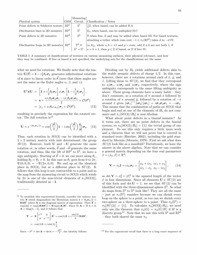
We summarize these and the results of the last threesections in Table IV.B.

V. BIAXIAL NEMATICS AND THE ODD HEDGEHOG

In the last section, we argued that by a smooth de-formation, a map from T2 to RP2 could absorb hedgehogcharge in pairs so that the hedgehog charge could only beeven or odd. Here, we probe this further and use the in-sight provided by decorating the uniaxial textures with asmall amount of biaxial order. This biaxial point of viewboth highlights the underlying topology of the uniaxialphase and clarifies the way in which the even and oddclasses of uniaxial disclination loops are distinct.

Recall in our discussion of the nematic we discovered,via some matrix algebra, that the ground state manifoldwas RP2. This was appropriate for a uniaxial nematic,which had rotational symmetry around its long axis – therotational symmetry responsible for the SO(2) factor inH. A biaxial nematic has a lower symmetry, that of abrick or rectangular cuboid with three unequal lengths.Not just a mathematical construct, biaxial liquid crys-talline phases have been known for many decades. In thepast few years, discovery of thermotropic biaxial phaseshas renewed interest in their defect structures. Moreover,

10 Free and based homotopy classes have the same classificationfor the first three classes where a, b are not both trivial, sincemultiplying by −1 doesn’t change evenness or oddness of thehedgehog charge on the islands. For the (+1,+1) case, the basedclassification is all integers, and the free classification is onlynonnegative integers, just as for textures on a sphere.

chirality and biaxiality are intimately connected (Har-ris, Kamien, and Lubensky, 1999; Priest and Lubensky,1974), and studies of blue phases (Dupuis, Marenduzzo,and Yeomans, 2005; Grebel, Hornreich, and Shtrikman,1983; Wright and Mermin, 1989) often utilize a biaxialdescription.

Returning to the notation and discussion in SectionII.C, we start with the biaxial molecule with long axisalong z and a second axis along x (the third axis is alongy and all three are distinguishable – “triaxial nematic”might be more apt). The symmetry of the brick involvesonly three discrete rotations of π around each of x, y,and z. Ignoring those symmetries for the moment, wesee that the original rotation matrices Rαβγ representan arbitrary rotation of the brick. With the symmetries,we must now identify γ with γ ± π, so that the isotropysubgroup Hb becomes

Hb = {1,P,Nπ,PNπ} , (10)

where the addition of elements (multiplication of the ma-trices) is as before. Note that PNπ = Mπ, so that a ro-tation around z of π followed by a similar rotation aboutx yields a π rotation around y. For all three of these ele-ments, we are never sure whether these rotations are by πor −π. Of course, the reader might think that these leadto the same group elements, which they do. However,a loop in SO(3) that starts at 0 rotation and ends at a2π rotation is not contractible and leads to a non-trivialelement of π1[SO(3)/Hb]. This fact, one might recall, isoften demonstrated in a class on quantum mechanics bysomeone who takes off their belt or holds a filled coffeecup with one hand and performs an elegant gyration oftheir arm11. It is why spinors must change sign underrotations by 2π and why the spin and statistics of par-ticles are interrelated. Now that we have introduced thenotion of a lift when discussing the hedgehog charge, itis simplest to demonstrate this fact with yet another lift.

The Pauli matrices:

σ1 =

[0 1

1 0

], σ2 =

[0 −ii 0

], σ3 =

[1 0

0 −1

], (11)

satisfy σiσj = iεijkσk + δij1 as follows from their com-mutators and anti-commutators. This can be used toform a simple way to parameterize rotations in three-dimensions. Write any vector ~x = [x1, x2, x3] as thematrix x = xkσk where we employ the summationconvention over repeated indices. Then x2 = |~x|21 isthe unit matrix times the squared length of the vec-tor. Moreover, if U is any 2 × 2 unitary matrix, thenif we define the similar matrix x′ = U†xU, we find that

(x′)2

= U†|~x|21U = x2 so under a unitary transforma-tion the magnitude of the matrix is unchanged, precisely

11 Some readers may have even been subjected to “spinor span-ners.”

16

MeasuringPhysical system GSM Circuit Classification / Notes

Point defects in Schlieren texture RP1 S1 12Z, when based, can be added II.A

Disclination lines in 3D nematics RP2 S1 Z2, when based, can be multiplied II.C

Point defects in 3D nematics RP2 S2 N when free, Z and may be added when based III. For based textures,

attaching a tether which runs over −1 ∈ π1(RP2) takes d to −d IV.

Disclination loops in 3D nematics RP2 T2 ∼= (a, b)p, where a, b = ±1 and p = even, odd if a, b are not both 1, if

S1 × S1 a = b = 1, then p ∈ Z if based, or N if free IV.

TABLE I A summary of classifications of textures on various measuring surfaces, their physical relevance, and howthey may be combined. If free or based is not specified, the underlying sets for the classifications are the same.

what we need for rotations. We finally note that the ma-

trix U(~θ) = 1− i 12θkσk generates infinitesimal rotations

of x since to linear order in ~θ (note that these angles arenot the same as the Euler angles α, β, and γ):

U†xU =

[1 + i

1

2θkσk

]xiσi

[1− i1

2θjσj

],

= x +ixiθkσkσi − ixiθkσiσk

2+O(θ2)

= [xj + xiθkεikj ]σj +O(θ2), (12)

resulting in precisely the expression for the rotated vec-tor. The full rotation is12

U = e−iθkσk/2 = cos

(|~θ|2

)1− i sin

(|~θ|2

)θk

|~θ|σk. (13)

Thus, each rotation in SO(3) can be identified with a2 × 2 unitary matrix with unit determinant, the groupSU(2). However, both U and −U generate the same

rotation or, in other words, ~θ and −~θ generate the samerotation, and thus, like the lift of RP2 to S2, we have a

sign ambiguity. Starting at ~θ = 0, we can move along θ1,holding θ2 = θ3 = 0. In this case as θ1 goes from 0 to 2π,U(0, 0, 0) = −U(2π, 0, 0). We end up at the identicalplace in SO(3), but at a different place in SU(2). Itfollows that this loop is not contractible to a point and sothe map from the measuring circuit to SO(3) which windsby 2π is one of the non-trivial elements of π1[SO(3)],traditionally denoted as −1.

12 To establish this exponential formula, consider the unitary ma-trix S which diagonalizes the Hermitian matrix t = θkσk/2 =SΛS† where Λ is the diagonal matrix of eigenvalues. Then T =exp{it} = exp{iSΛS†} = S exp{iΛ}S†. Since Tr Λ = Tr t = 0,Λ = diag[λ,−λ], and it follows that

T = S

[eiλ 0

0 e−iλ

]S† = cos(λ)1 + i

sin(λ)

λSΛS†,

= cos(λ)1 + i sin(λ)t

λ.

Since −λ2 = det Λ = det t = − |~θ|24

, the identity follows.

Dividing out by Hb yields additional defects akin tothe stable nematic defects of charge 1/2. In this case,however, there are π rotations around each of x, y, andz. Lifting those to SU(2), we find that they correspondto ±iσ1, ±iσ2 and ±iσ3, respectively, where the signambiguity corresponds to the same lifting ambiguity asabove. These group elements have a nasty habit – theydon’t commute, so a rotation of π around x followed bya rotation of π around y, followed by a rotation of −πaround x gives [iσ1]

−1[iσ2] [iσ1] = iσ1σ2σ1 = −iσ2.

This means that the combination of paths on SO(3) thatbegin and end at one of the elements of Hb do not com-mute and π1[SO(3)/Hb] is non-Abelian.

What about point defects in a biaxial nematic? Asit turns out, there are no point defects in the biaxialsystem, so π2[SO(3)/Hb] = {1} the trivial group of oneelement. To see this only requires a little more workand a theorem that we will not prove but is covered instandard texts (Hatcher, 2002), including the gold stan-dard by Mermin (Mermin, 1979). First we ask what doesSU(2) look like as a manifold? Fortuitously, we have theanswer in the above algebra. Note that we can considera general matrix depending on the four real parametersx = (x0, ~x) ∈ R4:

V = x01 + ixkσk =

[x0 + ix3 ix1 + x2ix1 − x2 x0 − ix3

], (14)

so detV = x20 + |~x|2 is the squared length of the vectorx in four dimensions. Since all elements U ∈ SU(2) areof this form and detU = 1, we see that SU(2) can beidentified with the three-dimensional sphere S3. So whatdo maps from S2 to S3 look like? They are all the same– just as π1(S2) vanishes because we can shrink everyloop on the sphere to a point, so too can we shrink everytwo-sphere on a three-sphere to a point. Thus π2(S3) =π2[SU(2)] = {1}. To calculate π2[SO[3]/Hb], we needonly use the theorem that π2(G) = π2(G/H) if H is adiscrete group13. Note that we saw this with S2 and RP2

– they both shared the same π2.

13 For the cognoscenti recall that there is a long exact sequence of

17

FIG. 9 Schematic of biaxial order on a colloid with radialanchoring conditions for the long axis. The two shorter axesundergo a 2π rotation at the North and South Poles and theparticle is threaded by a −1 disclination so that a Saturn ringdefect accompanying the colloid is linked with this biaxialdisclination.

Precisely because the biaxial nematic does not supportpoint defects, it serves to illuminate our previous discus-sion of disclination loops and their relation to hedgehogs.To see what we have gained it suffices to consider the sim-plest example: a disclination loop surrounding a singlecolloid in a Saturn ring configuration, illustrated in FIG.9. As usual the meridional cycle of a torus sheathing thedisclination records the non-trivial element of π1(RP2)and here, since the disclination is not linked with an-other, the longitudinal cycle records the trivial element.However, this cycle is still interesting. Note, in particu-lar, that the director field on the inside of the torus (thepart closest to the colloid) undergoes a 2π rotation as wetraverse this longitudinal cycle. Thus, if we were to deco-rate the uniaxial texture with a perpendicular short axisto produce a biaxial nematic we would find that this cy-cle corresponded to a non-contractible loop in SO(3)/Hb,recording the element −1 of π1(SO(3)/Hb). The Saturnring was linked with another disclination after all! An allbut invisible one only revealed by adding a small amountof biaxiality. This additional biaxial defect is not present

homotopy groups

. . .→ π2(H)→ π2(G)→ π2(G/H)→ π1(H)→ . . .

and if H is discrete then π2(H) = π1(H) = {1}, from which itfollows that π2(G) = π2(G/H).

for all defect loops: it is associated, as anticipated at theend of the last section, with a disclination loop that car-ries odd hedgehog charge, of which the Saturn ring is thesimplest example.

It is useful to explore this connection a little further.Suppose we remove the colloid, leaving behind just thedisclination loop and the texture on the torus surround-ing it. Could we fill things back in differently, say withoutthe hedgehog? Note that the configuration on the insideof the torus is just the same as on a cylindrical capillarywith perpendicular anchoring. Thus to avoid a singular-ity the director will have to escape in the third dimension,just as it does in a capillary. However, if we have biaxialorder then the singularity cannot be avoided; althoughthe long axis is well defined along the capillary axis thetwo shorter axes are not and we have a −1 disclination14.Let us assume that the texture is uniform at large dis-tances so that this defect too closes up to form a loop.Technically, we are considering textures with defects onS3, the usual three-dimensional Euclidean space with apoint at infinity added. The biaxial −1 disclination canalso be surrounded by a torus, whose meridian records a2π winding and longitude records the π winding of ouroriginal 1/2 loop with which it is linked. Now by escapingin the third dimension the long axis can be made regularon any local section of the −1 defect, but this cannotbe extended globally since the long axis is required toundergo a π rotation along any path encircling the 1/2disclination. This π rotation reverses the orientation ofthe director and converts an initial escape ‘up’ into anescape ‘down’ so that there must be a mismatch some-where. Just as in the cylindrical capillary this mismatchmarks the location of a point defect in the uniaxial ne-matic – the odd hedgehog.

VI. CONCLUSION

In the hope of avoiding to provide only a poor imita-tion of the many excellent reviews of the homotopy the-ory of defects already available, e.g. (Kurik and Lavren-tovich, 1988; Mermin, 1979; Michel, 1980; Trebin, 1982),we have focused our discussion on a single physical sys-tem, nematic liquid crystal colloids, rather than providea general survey and have eschewed, as far as possible,all of the formalities of algebraic topology.

A recurring issue is the necessity of a base point to in-duce the group structure on the set of homotopy classes.From a physical perspective the base point is really afiction, a convenience introduced for its useful compu-tational attributes rather than because it conveys anydeep significance. As mentioned in Section II the choiceof base point for this purpose is entirely arbitrary so that

14 This transferral of winding from one axis to a perpendicular oneis the celebrated Mermin-Ho relation (Mermin and Ho, 1976).

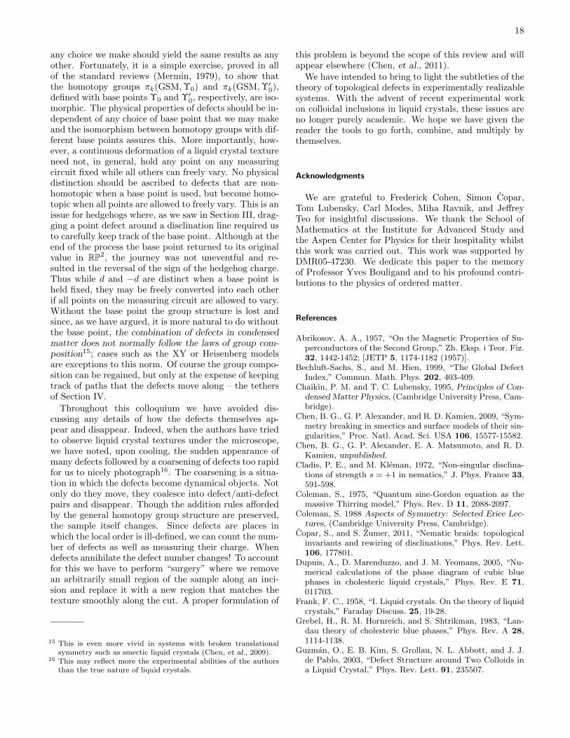
18

any choice we make should yield the same results as anyother. Fortunately, it is a simple exercise, proved in allof the standard reviews (Mermin, 1979), to show thatthe homotopy groups πk(GSM,Υ0) and πk(GSM,Υ′0),defined with base points Υ0 and Υ′0, respectively, are iso-morphic. The physical properties of defects should be in-dependent of any choice of base point that we may makeand the isomorphism between homotopy groups with dif-ferent base points assures this. More importantly, how-ever, a continuous deformation of a liquid crystal textureneed not, in general, hold any point on any measuringcircuit fixed while all others can freely vary. No physicaldistinction should be ascribed to defects that are non-homotopic when a base point is used, but become homo-topic when all points are allowed to freely vary. This is anissue for hedgehogs where, as we saw in Section III, drag-ging a point defect around a disclination line required usto carefully keep track of the base point. Although at theend of the process the base point returned to its originalvalue in RP2, the journey was not uneventful and re-sulted in the reversal of the sign of the hedgehog charge.Thus while d and −d are distinct when a base point isheld fixed, they may be freely converted into each otherif all points on the measuring circuit are allowed to vary.Without the base point the group structure is lost andsince, as we have argued, it is more natural to do withoutthe base point, the combination of defects in condensedmatter does not normally follow the laws of group com-position15; cases such as the XY or Heisenberg modelsare exceptions to this norm. Of course the group compo-sition can be regained, but only at the expense of keepingtrack of paths that the defects move along – the tethersof Section IV.

Throughout this colloquium we have avoided dis-cussing any details of how the defects themselves ap-pear and disappear. Indeed, when the authors have triedto observe liquid crystal textures under the microscope,we have noted, upon cooling, the sudden appearance ofmany defects followed by a coarsening of defects too rapidfor us to nicely photograph16. The coarsening is a situa-tion in which the defects become dynamical objects. Notonly do they move, they coalesce into defect/anti-defectpairs and disappear. Though the addition rules affordedby the general homotopy group structure are preserved,the sample itself changes. Since defects are places inwhich the local order is ill-defined, we can count the num-ber of defects as well as measuring their charge. Whendefects annihilate the defect number changes! To accountfor this we have to perform “surgery” where we removean arbitrarily small region of the sample along an inci-sion and replace it with a new region that matches thetexture smoothly along the cut. A proper formulation of

15 This is even more vivid in systems with broken translationalsymmetry such as smectic liquid crystals (Chen, et al., 2009).

16 This may reflect more the experimental abilities of the authorsthan the true nature of liquid crystals.

this problem is beyond the scope of this review and willappear elsewhere (Chen, et al., 2011).

We have intended to bring to light the subtleties of thetheory of topological defects in experimentally realizablesystems. With the advent of recent experimental workon colloidal inclusions in liquid crystals, these issues areno longer purely academic. We hope we have given thereader the tools to go forth, combine, and multiply bythemselves.

Acknowledgments

We are grateful to Frederick Cohen, Simon Copar,Tom Lubensky, Carl Modes, Miha Ravnik, and JeffreyTeo for insightful discussions. We thank the School ofMathematics at the Institute for Advanced Study andthe Aspen Center for Physics for their hospitality whilstthis work was carried out. This work was supported byDMR05-47230. We dedicate this paper to the memoryof Professor Yves Bouligand and to his profound contri-butions to the physics of ordered matter.

References

Abrikosov, A. A., 1957, “On the Magnetic Properties of Su-perconductors of the Second Group,” Zh. Eksp. i Teor. Fiz.32, 1442-1452; [JETP 5, 1174-1182 (1957)].

Bechluft-Sachs, S., and M. Hien, 1999, “The Global DefectIndex,” Commun. Math. Phys. 202, 403-409.

Chaikin, P. M. and T. C. Lubensky, 1995, Principles of Con-densed Matter Physics, (Cambridge University Press, Cam-bridge).

Chen, B. G., G. P. Alexander, and R. D. Kamien, 2009, “Sym-metry breaking in smectics and surface models of their sin-gularities,” Proc. Natl. Acad. Sci. USA 106, 15577-15582.

Chen, B. G., G. P. Alexander, E. A. Matsumoto, and R. D.Kamien, unpublished.

Cladis, P. E., and M. Kleman, 1972, “Non-singular disclina-tions of strength s = +1 in nematics,” J. Phys. France 33,591-598.

Coleman, S., 1975, “Quantum sine-Gordon equation as themassive Thirring model,” Phys. Rev. D 11, 2088-2097.

Coleman, S. 1988 Aspects of Symmetry: Selected Erice Lec-tures, (Cambridge University Press, Cambridge).

Copar, S., and S. Zumer, 2011, “Nematic braids: topologicalinvariants and rewiring of disclinations,” Phys. Rev. Lett.106, 177801.

Dupuis, A., D. Marenduzzo, and J. M. Yeomans, 2005, “Nu-merical calculations of the phase diagram of cubic bluephases in cholesteric liquid crystals,” Phys. Rev. E 71,011703.

Frank, F. C., 1958, “I. Liquid crystals. On the theory of liquidcrystals,” Faraday Discuss. 25, 19-28.

Grebel, H., R. M. Hornreich, and S. Shtrikman, 1983, “Lan-dau theory of cholesteric blue phases,” Phys. Rev. A 28,1114-1138.

Guzman, O., E. B. Kim, S. Grollau, N. L. Abbott, and J. J.de Pablo, 2003, “Defect Structure around Two Colloids ina Liquid Crystal,” Phys. Rev. Lett. 91, 235507.

19

Harris, A. B., R. D. Kamien, and T. C. Lubensky, 1999,“Molecular chirality and chiral parameters,” Rev. Mod.Phys. 71, 1745-1757.

Hatcher, A., 2002, Algebraic Topology, Cambridge UniversityPress, Cambridge.

Janich, K., 1987, “Topological properties of ordinary nematicsin 3-space,” Acta Appl. Math. 8, 65-74.

Kamien, R. D., 2002, “The geometry of soft materials: Aprimer,” Rev. Mod. Phys. 74, 953-971.

Kamien, R. D., 2011, “Knot your simple defect lines,” Science333, 46-47.

Kitaev, A. Yu., 2003, “Fault-tolerant quantum computationby anyons,” Ann. Phys. 303, 2-30.

Kosterlitz, J. M., and D. J. Thouless, 1973, “Ordering,metastability and phase transitions in two-dimensional sys-tems,” J. Phys. C: Solid State Phys., 6, 1181-1203.

Kurik, M. V., and O. D. Lavrentovich, 1988, “Defects in liq-uid crystals: homotopy theory and experimental studies,”Phys. Usp. 31, 196-224.

Lintuvuori, J. S., D. Marenduzzo, K. Stratford, and M. E.Cates, 2010, “Colloids in liquid crystals: a lattice Boltz-mann study,” J. Mater. Chem. 20, 10547-10552.

Mermin, N. D., 1979, “The topological theory of defects inordered media,” Rev. Mod. Phys. 51, 591-648.

Mermin, N. D, and T. L. Ho, 1976, “Circulation and angularmomentum in the A phase of superfluid Helium-3,” Phys.Rev. Lett. 36, 594-597; 36, 832(E).

Meyer, R. B., 1973, “On the existence of even indexed discli-nations in nematic liquid crystals,” Phil. Mag. 27, 405-424.

Michel, L., 1980, “Symmetry defects and broken symmetry.Configurations hidden symmetry,” Rev. Mod. Phys. 52,617-651.

Muhlbauer, S., B. Binz, F. Jonitez, C. Pfleiderer, A. Rosch,A. Neubauer, R. Georgii, and P. Boni, 2009, “SkyrmionLattice in a Chiral Magnet,” Science 323, 915-919.

Musevic, I., M. Skarabot, U. Tkalec, M. Ravnik, and S.Zumer, 2006, “Two-dimensional nematic colloidal crystalsself-assembled by topological defects,” Science 313, 954-958.

Nakanishi, H., K. Hayashi, and H. Mori, 1988, “Topologicalclassification of unknotted ring defects,” Commun. Math.Phys. 117, 203-213.

Nayak, C., S. H. Simon, A. Stern, M. Freedman, and S. DasSarma, 2008, “Non-Abelian anyons and topological quan-tum computation,” Rev. Mod. Phys. 80, 1083-1159.

Nelson, D. R., 1988, “Vortex Entanglement in High-Tc Super-

conductors,” Phys. Rev. Lett. 60, 1973-1976.Poenaru, V., and G. Toulouse, 1977, “The crossing of defects

in ordered media and the topology of 3-manifolds,” J. Phys.France 38, 887-895.

Polyakov, A. M., 1974, “Particle spectrum in quantum fieldtheory,” ZhETF Pis. Red. 20, 430-433; [JETP 20, 194-195(1974)].

Poulin, P., H. Stark, T. C. Lubensky, and D. A. Weitz, 1997,“Novel Colloidal Interactions in Anisotropic Fluids,” Sci-ence 275, 1770-1773.

Priest, R. G. and T. C. Lubensky, 1974, “Biaxial model ofcholesteric liquid crystals,” Phys. Rev. A 9 893-898.

Ravnik, M., M. Skarabot, S. Zumer, U. Tkalec, I. Poberaj,D. Babic, N. Osterman, and I. Musevic, 2007, “EntangledNematic Colloidal Dimers and Wires,” Phys. Rev. Lett. 99,247801.

Ravnik, M., and S. Zumer, 2009, “Nematic colloids entangledby topological defects,” Soft Matter 5, 269-274.

Roßler, U. K., A. N. Bogdanov, and C. Pfleiderer, 2006,“Spontaneous skyrmion ground states in magnetic metals,”Nature 442, 797-801.

Skarabot, M., M. Ravnik, S. Zumer, U. Tkalec, I. Poberaj,D. Babic, N. Osterman, and I. Musevic, 2007, “Two-dimensional dipolar nematic colloidal crystals,” Phys. Rev.E 76, 051406.

Skarabot, M., M. Ravnik, S. Zumer, U. Tkalec, I. Poberaj, D.Babic, N. Osterman, and I. Musevic, 2008, “Interactions ofquadrupolar nematic colloids,” Phys. Rev. E 77, 031705.

Smalyukh, I. I., Y. Lansac, N. A. Clark, and R. P. Trivedi,2009, “Three-dimensional structure and multistable opti-cal switching of triple-twisted particle-like excitations inanisotropic fluids,” Nat. Mater. 9, 1-7.

Terentjev, E. M., 1995, “Disclination loops, standing aloneand around solid particles, in nematic liquid crystals,”Phys. Rev. E 51, 1330-1337.

Tkalec, U., M. Ravnik, S. Copar, S. Zumer, and I. Musevic,2011, “Reconfigurable knots and links in chiral nematic col-loids,” Science 333, 62-65.

Trebin, H. R., 1982, “The topology of non-uniform media incondensed matter physics,” Adv. Phys. 31, 195-254.

Williams, C., and Y. Bouligand, 1974, “Fils et disinclinaisonsdans un nematique en tube capillaire,” J. Phys. France 35,589-593.

Wright, D. C. and N. D. Mermin, 1989, “Crystalline liquids:the blue phases,” Rev. Mod. Phys. 61, 385-432.