DisC Diversity: Result Diversification based onDissimilarity and Coverage ∗

Marina DrosouComputer Science DepartmentUniversity of Ioannina, Greece

mdrosou@cs.uoi.gr

Evaggelia PitouraComputer Science DepartmentUniversity of Ioannina, Greece

pitoura@cs.uoi.gr

ABSTRACTRecently, result diversification has attracted a lot of atten-tion as a means to improve the quality of results retrieved byuser queries. In this paper, we propose a new, intuitive defi-nition of diversity called DisC diversity. A DisC diverse sub-set of a query result contains objects such that each objectin the result is represented by a similar object in the diversesubset and the objects in the diverse subset are dissimilarto each other. We show that locating a minimum DisC di-verse subset is an NP-hard problem and provide heuristicsfor its approximation. We also propose adapting DisC di-verse subsets to a different degree of diversification. We callthis operation zooming. We present efficient implementa-tions of our algorithms based on the M-tree, a spatial indexstructure, and experimentally evaluate their performance.

1. INTRODUCTIONResult diversification has attracted considerable attention

as a means of enhancing the quality of query results pre-sented to users (e.g.,[26, 32]). Consider, for example, a userwho wants to buy a camera and submits a related query. Adiverse result, i.e., a result containing various brands andmodels with different pixel counts and other technical char-acteristics is intuitively more informative than a homoge-neous result containing only cameras with similar features.

There have been various definitions of diversity [10], basedon (i) content (or similarity), i.e., objects that are dissim-ilar to each other (e.g., [32]), (ii) novelty, i.e., objects thatcontain new information when compared to what was pre-viously presented (e.g., [9]) and (iii) semantic coverage, i.e.,objects that belong to different categories or topics (e.g.,[3]). Most previous approaches rely on assigning a diversityscore to each object and then selecting either the k objectswith the highest score for a given k (e.g., [4, 14]) or theobjects with score larger than some threshold (e.g., [29]).

In this paper, we address diversity through a differentperspective. Let P be the set of objects in a query result.We consider two objects p1 and p2 in P to be similar, if

∗This paper has been granted the Reproducible Label by theVLDB 2013 reproducibility committee. More informationconcerning our evaluation system and experimental resultscan be found at http://www.dbxr.org.

Permission to make digital or hard copies of all or part of this work forpersonal or classroom use is granted without fee provided that copies arenot made or distributed for profit or commercial advantage and that copiesbear this notice and the full citation on the first page. To copy otherwise, torepublish, to post on servers or to redistribute to lists, requires prior specificpermission and/or a fee. Articles from this volume were invited to presenttheir results at The 39th International Conference on Very Large Data Bases,August 26th - 30th 2013, Riva del Garda, Trento, Italy.Proceedings of the VLDB Endowment, Vol. 6, No. 1Copyright 2012 VLDB Endowment 2150-8097/12/11...$ 10.00.

dist(p1, p2) ≤ r for some distance function dist and realnumber r, where r is a tuning parameter that we call radius.Given P, we select a representative subset S ⊆ P to bepresented to the user such that: (i) all objects in P aresimilar with at least one object in S and (ii) no two objectsin S are similar with each other. The first condition ensuresthat all objects in P are represented, or covered, by at leastone object in the selected subset. The second conditionensures that the selected objects of P are dissimilar. Wecall the set S r-Dissimilar and Covering subset or r-DisCdiverse subset.

In contrary to previous approaches to diversification, weaim at computing subsets of objects that contain objectsthat are both dissimilar with each other and cover the wholeresult set. Furthermore, instead of specifying a requiredsize k of the diverse set or a threshold, our tuning pa-rameter r explicitly expresses the degree of diversificationand determines the size of the diverse set. Increasing r re-sults in smaller, more diverse subsets, while decreasing rresults in larger, less diverse subsets. We call these oper-ations, zooming-out and zooming-in respectively. One canalso zoom-in or zoom-out locally to a specific object in thepresented result.

As an example, consider searching for cities in Greece.Figure 1 shows the results of this query diversified based ongeographical location for an initial radius (a), after zooming-in (b), zooming-out (c) and local zooming-in a specific city(d). As another example of local zooming in the case ofcategorical attributes, consider looking for cameras, wherediversity refers to cameras with different features. Figure 2depicts an initial most diverse result and the result of localzooming-in one individual camera in this result.

We formalize the problem of locating minimum DisC di-verse subsets as an independent dominating set problem ongraphs [17]. We provide a suite of heuristics for computingsmall DisC diverse subsets. We also consider the problem ofadjusting the radius r. We explore the relation among DisCdiverse subsets of different radii and provide algorithms forincrementally adapting a DisC diverse subset to a new ra-dius. We provide theoretical upper bounds for the size ofthe diverse subsets produced by our algorithms for com-puting DisC diverse subsets as well as for their zoomingcounterparts. Since the crux of the efficiency of the pro-posed algorithms is locating neighbors, we take advantageof spatial data structures. In particular, we propose efficientalgorithms based on the M-tree [30].

We compare the quality of our approach to other diver-sification methods both analytically and qualitatively. Wealso evaluate our various heuristics using both real and syn-thetic datasets. Our performance results show that the ba-sic heuristic for computing dissimilar and covering subsetsworks faster than its greedy variation but produces largersets. Relaxing the dissimilarity condition, although in the-ory could result in smaller sets, in our experiments does not

13

(a) Initial set. (b) Zooming-in.

(c) Zooming-out. (d) Local zooming-in.

Figure 1: Zooming. Selected objects are shown inbold. Circles denote the radius r around the se-lected objects.

reduce the size of the result considerably. Our incrementalalgorithms for zooming in or out from r to a different radiusr′, when compared to computing a DisC diverse subset forr′ from scratch, produce sets of similar sizes and closer towhat the user intuitively expects, while imposing a smallercomputational cost. Finally, we draw various conclusionsfor the M-tree implementation of these algorithms.

Most often diversification is modeled as a bi-criteria prob-lem with the dual goal of maximizing both the diversity andthe relevance of the selected results. In this paper, we focussolely on diversity. Since we “cover” the whole dataset, eachuser may “zoom-in” to the area of the results that seemsmost relevant to her individual needs. Of course, many otherapproaches to integrating relevance with DisC diversity arepossible; we discuss some of them in Section 8.

In a nutshell, in this paper, we make the following contri-butions:

– we propose a new, intuitive definition of diversity, calledDisC diversity and compare it with other models,

– we show that locating minimum DisC diverse subsetsis an NP-hard problem and provide efficient heuristicsalong with approximation bounds,

– we introduce adaptive diversification through zooming-in and zooming-out and present algorithms for theirincremental computation as well as corresponding the-oretical bounds,

– we provide M-tree tailored algorithms and experimen-tally evaluate their performance.

The rest of the paper is structured as follows. Section 2introduces DisC diversity and heuristics for computing smalldiverse subsets, Section 3 introduces adaptive diversificationand Section 4 compares our approach with other diversifi-cation methods. In Section 5, we employ the M-tree forthe efficient implementation of our algorithms, while in Sec-tion 6, we present experimental results. Finally, Section 7presents related work and Section 8 concludes the paper.

2. DISC DIVERSITYIn this section, we first provide a formal definition of DisC

diversity. We then show that locating a minimum DisCdiverse set of objects is an NP-hard problem and presentheuristics for locating approximate solutions.

Brand Model Megapixels Zoom Interface Battery Storage

Epson PhotoPC 750Z 1.2 3.0 serial NiMH internal, CompactFlash

Ricoh RDC-5300 2.2 3.0 serial, USB AA internal, SmartMedia

Sony Mavica DSC-D700 1.4 5.0 None lithium MemoryStick

Pentax Optio 33WR 3.1 2.8 USB AA, lithium MultiMediaCard, SecureDigital

Toshiba PDR-M11 1.2 no USB AA SmartMedia

FujiFilm MX-1700 1.3 3.2 serial lithium SmartMedia

FujiFilm FinePix S20 Pro 6.0 6.0 USB, FireWire AA xD-PictureCard

Nikon Coolpix 600 0.8 no serial NiCd CompactFlash

Canon IXUS 330 1.9 3.0 USB lithium CompactFlash

Brand Model Megapixels Zoom Interface Battery Storage

Canon S30 IS 14.0 35.0 USB lithium SecureDigital, SecureDigital HC

Canon A520 3.9 4.0 USB AA MultiMediaCard, SecureDigital

Canon A400 3.1 2.2 USB AA SecureDigital

Canon ELPH Sd10 3.9 no USB lithium SecureDigital

Canon A200 1.9 no USB AA CompactFlash

Canon S30 3.0 3.0 USB lithium CompactFlash

Figure 2: Zooming in a specific camera.

2.1 Definition of DisC DiversityLet P be a set of objects returned as the result of a user

query. We want to select a representative subset S of theseobjects such that each object from P is represented by asimilar object in S and the objects selected to be includedin S are dissimilar to each other.

We define similarity between two objects using a distancemetric dist. For a real number r, r ≥ 0, we use Nr(pi) todenote the set of neighbors (or neighborhood) of an objectpi ∈ P, i.e., the objects lying at distance at most r from pi:

Nr(pi) = {pj | pi 6= pj ∧ dist(pi, pj) ≤ r}We use N+

r (pi) to denote the set Nr(pi) ∪ {pi}, i.e., theneighborhood of pi including pi itself. Objects in the neigh-borhood of pi are considered similar to pi, while objectsoutside its neighborhood are considered dissimilar to pi. Wedefine an r-DisC diverse subset as follows:

Definition 1. (r-DisC Diverse Subset) Let P be aset of objects and r, r ≥ 0, a real number. A subset S ⊆ Pis an r-Dissimilar-and-Covering diverse subset, or r-DisCdiverse subset, of P, if the following two conditions hold:(i) (coverage condition) ∀pi ∈ P, ∃pj ∈ N+

r (pi), such thatpj ∈ S and (ii) (dissimilarity condition) ∀ pi, pj ∈ S withpi 6= pj, it holds that dist(pi, pj) > r.

The first condition ensures that all objects in P are rep-resented by at least one similar object in S and the secondcondition that the objects in S are dissimilar to each other.We call each object pi ∈ S an r-DisC diverse object and rthe radius of S. When the value of r is clear from context,we simply refer to r-DisC diverse objects as diverse objects.Given P, we would like to select the smallest number ofdiverse objects.

Definition 2. (The Minimum r-DisC Diverse Subset

Problem) Given a set P of objects and a radius r, find anr-DisC diverse subset S∗ of P, such that, for every r-DisCdiverse subset S of P, it holds that |S∗| ≤ |S|.

In general, there may be more than one minimum r-DisCdiverse subsets of P (see Figure 3(a) for an example).

2.2 Graph Representation and NP-hardnessLet us consider the following graph representation of a set

P of objects. Let GP,r = (V , E) be an undirected graphsuch that there is a vertex vi ∈ V for each object pi ∈ P andan edge (vi, vj) ∈ E, if and only if, dist(pi, pj) ≤ r for thecorresponding objects pi, pj , pi 6= pj . An example is shownin Figure 3(b).

Let us recall a couple of graph-related definitions. A dom-inating set D for a graph G is a subset of vertices of G suchthat every vertex of G not in D is joined to at least onevertex of D by some edge. An independent set I for a graph

14

p

pp p

p

p

p

(a)

v1

v3

v2

v4

v6

v5

v7

(b)

Figure 3: (a) Minimum r-DisC diverse subsetsfor the depicted objects: {p

1, p

4, p

7}, {p

2, p

4, p

7},

{p3, p

5, p

6}, {p

3, p

5, p

7} and (b) their graph represen-

tation.

G is a set of vertices of G such that for every two vertices inI, there is no edge connecting them. It is easy to see thata dominating set of GP,r satisfies the covering conditions ofDefinition 1, whereas an independent set of GP,r satisfiesthe dissimilarity conditions of Definition 1. Thus:

Observation 1. Solving the Minimum r-DisC Diverse

Subset Problem for a set P is equivalent to finding a Min-

imum Independent Dominating Set of the correspondinggraph GP,r.

The Minimum Independent Dominating Set Problem

has been proven to be NP-hard [15]. The problem remainsNP-hard even for special kinds of graphs, such as for unitdisk graphs [8]. Unit disk graphs are graphs whose verticescan be put in one to one correspondence with equisized cir-cles in a plane such that two vertices are joined by an edge,if and only if, the corresponding circles intersect. GP,r is aunit disk graph for Euclidean distances.

In the following, we use the terms dominance and cover-age, as well as, independence and dissimilarity interchange-ably. In particular, two objects pi and pj are independent, ifdist(pi, pj) > r. We also say that an object covers all objectsin its neighborhood. We next present some useful propertiesthat relate the coverage (i.e., dominance) and dissimilarity(i.e., independence) conditions. A maximal independent setis an independent set such that adding any other vertex tothe set forces the set to contain an edge, that is, it is an in-dependent set that is not a subset of any other independentset. It is known that:

Lemma 1. An independent set of a graph is maximal, ifand only if, it is dominating.

From Lemma 1, we conclude that:Observation 2. A minimum maximal independent set is

also a minimum independent dominating set.However,

Observation 3. A minimum dominating set is not nec-essarily independent.

For example, in Figure 4, the minimum dominating set ofthe depicted objects is of size 2, while the minimum inde-pendent dominating set is of size 3.

2.3 Computing DisC Diverse ObjectsWe consider first a baseline algorithm for computing a

DisC diverse subset S of P. For presentation convenience,let us call black the objects of P that are in S, grey theobjects covered by S and white the objects that are neitherblack nor grey. Initially, S is empty and all objects are white.The algorithm proceeds as follows: until there are no morewhite objects, it selects an arbitrary white object pi, colorspi black and colors all objects in Nr(pi) grey. We call thisalgorithm Basic-DisC.

The produced set S is clearly an independent set, sinceonce an object enters S, all its neighbors become grey andthus are withdrawn from consideration. It is also a maxi-mal independent set, since at the end there are only grey

v v

v

v v

v

(a)

v v

v

v v

v

(b)

Figure 4: (a) Minimum dominating set ({v2, v5})and (b) a minimum independent dominating set({v2, v4, v6}) for the depicted graph.

objects left, thus adding any of them to S would violate theindependence of S. From Lemma 1, the set S produced byBasic-DisC is an r-DisC diverse subset. S is not necessarilya minimum r-DisC diverse subset. However, its size is re-lated to the size of any minimum r-DisC diverse subset S∗

as follows:

Theorem 1. Let B be the maximum number of indepen-dent neighbors of any object in P. Any r-DisC diverse subsetS of P is at most B times larger than any minimum r-DisCdiverse subset S∗.

Proof. Since S is an independent set, any object in S∗

can cover at most B objects in S and thus |S| ≤ B|S∗|.The value of B depends on the distance metric used and

also on the dimensionality d of the data space. For manydistance metrics B is a constant. Next, we show how Bis bounded for specific combinations of the distance metricdist and data dimensionality d.

Lemma 2. If dist is the Euclidean distance and d = 2,each object pi in P has at most 5 neighbors that are inde-pendent from each other.

Proof. Let p1, p2 be two independent neighbors of pi.Then, it must hold that ∠p1pip2 is larger than π

3. Other-

wise, dist(p1, p2) ≤ max{dist(pi, p1), dist(pi, p2)} ≤ r whichcontradicts the independence of p1 and p2. Therefore, pi canhave at most (2π/π

3) − 1 = 5 independent neighbors.

Lemma 3. If dist is the Manhattan distance and d = 2,each object pi in P has at most 7 neighbors that are inde-pendent from each other.

Proof. The proof can be found in the Appendix.

Also, for d = 3 and the Euclidean distance, it can beshown that each object pi in P has at most 24 neighborsthat are independent from each other. This can be shownusing packing techniques and properties of solid angles [11].

We now consider the following intuitive greedy variationof Basic-DisC, that we call Greedy-DisC. Instead of select-ing white objects arbitrarily at each step, we select the whiteobject with the largest number of white neighbors, that is,the white object that covers the largest number of uncov-ered objects. Greedy-DisC is shown in Algorithm 1, whereNW

r (pi) is the set of the white neighbors of object pi.While the size of the r-DisC diverse subset S produced

by Greedy-DisC is expected to be smaller than that of thesubset produced by Basic-DisC, the fact that we considerfor inclusion in S only white, i.e., independent, objects maystill not reduce the size of S as much as expected. FromObservation 3, it is possible that an independent coveringset is larger than a covering set that also includes dependentobjects. For example, consider the nodes (or equivalentlythe corresponding objects) in Figure 4. Assume that objectv2 is inserted in S first, resulting in objects v1, v3 and v5

becoming grey. Then, we need two more objects, namely, v4

and v6, for covering all objects. However, if we consider forinclusion grey objects as well, then v5 can join S, resultingin a smaller covering set.

15

Algorithm 1 Greedy-DisC

Input: A set of objects P and a radius r.Output: An r-DisC diverse subset S of P.

1: S ← ∅2: for all pi ∈ P do3: color pi white4: end for5: while there exist white objects do

6: select the white object pi with the largest∣

∣NWr (pi)

∣

∣

7: S = S ∪ {pi}8: color pi black9: for all pj ∈ NW

r (pi) do

10: color pj grey11: end for12: end while13: return S

Motivated by this observation, we also define r-C diversesubsets that satisfy only the coverage condition of Defini-tion 1 and modify Greedy-DisC accordingly to compute r-Cdiverse sets. The only change required is that in line 6 ofAlgorithm 1, we select both white and grey objects. Thisallows us to select at each step the object that covers thelargest possible number of uncovered objects, even if thisobject is grey. We call this variation Greedy-C. In the caseof Greedy-C, we prove the following bound for the size ofthe produced r-C diverse subset S:

Theorem 2. Let ∆ be the maximum number of neigh-bors of any object in P. The r-C diverse subset producedby Greedy-C is at most ln ∆ times larger than the minimumr-DisC diverse subset S∗.

Proof. The proof can be found in the Appendix.

3. ADAPTIVE DIVERSIFICATIONThe radius r determines the desired degree of diversifica-

tion. A large radius corresponds to fewer and less similar toeach other representative objects, whereas a small radius re-sults in more and less dissimilar representative objects. Onone extreme, a radius equal to the largest distance betweenany two objects results in a single object being selected andon the other extreme, a zero radius results in all objects ofP being selected. We consider an interactive mode of op-eration where, after being presented with an initial set ofresults for some r, a user can see either more or less resultsby correspondingly decreasing or increasing r.

Specifically, given a set of objects P and an r-DisC diversesubset Sr of P, we want to compute an r′-DisC diverse

subset Sr′

of P. There are two cases: (i) r′ < r and (ii) r′ >r which we call zooming-in and zooming-out respectively.These operations are global in the sense that the radius r ismodified similarly for all objects in P. We may also modifythe radius for a specific area of the data set. Consider, forexample, a user that receives an r-DisC diverse subset Sr

of the results and finds some specific object pi ∈ Sr moreor less interesting. Then, the user can zoom-in or zoom-out by specifying a radius r′, r′ < r or r′ > r, respectively,centered in pi. We call these operations local zooming-in andlocal zooming-out respectively.

To study the size relationship between Sr and Sr′

, wedefine the set NI

r1,r2(pi), r2 ≥ r1, as the set of objects at

distance at most r2 from pi which are at distance at leastr1 from each other, i.e., objects in Nr2

(pi)\Nr1(pi) that are

independent from each other considering the radius r1. Thefollowing lemma bounds the size of NI

r1,r2(pi) for specific

distance metrics and dimensionality.

Lemma 4. Let r1, r2 be two radii with r2 ≥ r1. Then, ford = 2:

p1

r

r׳p4

p5

p3

p2

(a)

p1p2

rr׳

p3

p5

p4

(b)

Figure 5: Zooming (a) in and (b) out. Solid anddashed circles correspond to radius r

′ and r respec-tively.

(i) if dist is the Euclidean distance:∣

∣

∣NI

r1,r2(pi)

∣

∣

∣≤ 9

⌈

logβ(r2/r1)⌉

, where β =1 +

√5

2

(ii) if dist is the Manhattan distance:∣

∣

∣NI

r1,r2(pi)

∣

∣

∣≤ 4

γ∑

i=1

(2i + 1), where γ =

⌈

r2 − r1

r1

⌉

Proof. The proof can be found in the Appendix.

Since we want to support an incremental mode of opera-

tion, the set Sr′

should be as close as possible to the already

seen result Sr. Ideally, Sr′ ⊇ Sr, for r′ < r and Sr′ ⊆ Sr,

for r′ > r. We would also like the size of Sr′

to be as close aspossible to the size of the minimum r′-DisC diverse subset.

If we consider only the coverage condition, that is, onlyr-C diverse subsets, then an r-C diverse subset of P is alsoan r′-C diverse subset of P, for any r′ ≥ r. This holdsbecause Nr(pi) ⊆ Nr′(pi) for any r′ ≥ r. However, a similarproperty does not hold for the dissimilarity condition. Ingeneral, a maximal independent diverse subset Sr of P forr is not necessarily a maximal independent diverse subset ofP, neither for r′ > r nor for r′ < r. To see this, note thatfor r′ > r, Sr may not be independent, whereas for r′ < r,Sr may no longer be maximal. Thus, from Lemma 1, wereach the following conclusion:

Observation 4. In general, there is no monotonic prop-erty among the r-DisC diverse and the r′-DisC diverse sub-sets of a set of objects P, for r 6= r′.

For zooming-in, i.e., for r′ < r, we can construct r′-DisCdiverse sets that are supersets of Sr by adding objects toSr to make it maximal. For zooming-out, i.e., for r′ >r, in general, there may be no subset of Sr that is r′-DisCdiverse. Take for example the objects of Figure 5(b) with Sr

= {p1, p2, p3}. No subset of Sr is an r′-DisC diverse subsetfor this set of objects. Next, we detail the zooming-in andzooming-out operations.

3.1 Incremental Zooming-inLet us first consider the case of zooming with a smaller

radius, i.e., r′ < r. Here, we aim at producing a small

independent covering solution Sr′

, such that, Sr′ ⊇ Sr. Forthis reason, we keep the objects of Sr in the new r′-DisC

diverse subset Sr′

and proceed as follows.Consider an object of Sr, for example p1 in Figure 5(a).

Objects at distance at most r′ from p1 are still covered by

p1 and cannot enter Sr′

. Objects at distance greater than r′

and at most r may be uncovered and join Sr′

. Each of these

objects can enter Sr′

as long as it is not covered by someother object of Sr that lays outside the former neighborhood

of p1. For example, in Figure 5(a), p4 and p5 may enter Sr′

16

Algorithm 2 Greedy-Zoom-In

Input: A set of objects P, an initial radius r, a solution Sr anda new radius r′ < r.

Output: An r′-DisC diverse subset of P.

1: Sr′

← Sr

2: for all pi ∈ Sr do3: color objects in {Nr(pi)\Nr′ (pi)} white4: end for5: while there exist white objects do

6: select the white object pi with the largest∣

∣NWr (pi)

∣

∣

7: color pi black

8: Sr′

= Sr′

∪ {pi}9: for all pj ∈ NW

r (pi) do

10: color pj grey11: end for12: end while

13: return Sr′

while p3 can not, since, even with the smaller radius r′, p3

is covered by p2.To produce an r′-DisC diverse subset based on an r-DisC

diverse subset, we consider such objects in turn. This turncan be either arbitrary (Basic-Zoom-In algorithm) or pro-ceed in a greedy way, where at each turn the object thatcovers the largest number of uncovered objects is selected(Greedy-Zoom- In, Algorithm 2).

Lemma 5. For the set Sr′

generated by the Basic-Zoom-Inand Greedy-Zoom-In algorithms, it holds that:

(i) Sr ⊆ Sr′

and

(ii) |Sr′ | ≤ NIr′,r(pi)|Sr|

Proof. Condition (i) trivially holds from step 1 of thealgorithm. Condition (ii) holds since for each object in Sr

there are at most NIr′,r(pi) independent objects at distance

greater than r′ from each other that can enter Sr′

.

In practice, objects selected to enter Sr′

, such as p4 and p5

in Figure 5(a), are likely to cover other objects left uncoveredby the same or similar objects in Sr. Therefore, the size

difference between Sr and Sr′

is expected to be smaller thanthis theoretical upper bound.

3.2 Incremental Zooming-outNext, we consider zooming with a larger radius, i.e., r′ >

r. In this case, the user is interested in seeing less andmore dissimilar objects, ideally a subset of the already seen

results for r, that is, Sr′ ⊆ Sr. However, in this case, asdiscussed, in contrast to zooming-in, it may not be possible

to construct a diverse subset Sr′

that is a subset of Sr.Thus, we focus on the following sets of objects: (i) Sr\Sr′

and (ii) Sr′\Sr. The first set consists of the objects thatbelong to the previous diverse subset but are removed fromthe new one, while the second set consists of the new ob-

jects added to Sr′

. To illustrate, let us consider the objectsof Figure 5(b) and that p1, p2, p3 ∈ Sr. Since the radiusbecomes larger, p1 now covers all objects at distance at mostr′ from it. This may include a number of objects that alsobelonged to Sr, such as p2. These objects have to be re-moved from the solution, since they are no longer dissimilarto p1. However, removing such an object, say p2 in our ex-ample, can potentially leave uncovered a number of objectsthat were previously covered by p2 (these objects lie in theshaded area of Figure 5(b)). In our example, requiring p1 to

remain in Sr′

means than p5 should be now added to Sr′

.To produce an r′-DisC diverse subset based on an r-DisC

diverse subset, we proceed in two passes. In the first pass,

Algorithm 3 Greedy-Zoom-Out(a)

Input: A set of objects P, an initial radius r, a solution Sr anda new radius r′ > r.

Output: An r′-DisC diverse subset of P.

1: Sr′

← ∅2: color all black objects red3: color all grey objects white4: while there exist red objects do

5: select the red object pi with the largest |NRr′ (pi)|

6: color pi black

7: Sr′

= Sr′

∪ {pi}8: for all pj ∈ Nr′ (pi) do

9: color pj grey10: end for11: end while12: while there exist white objects do

13: select the white object pi with the larger |NWr′ (pi)|

14: color pi black

15: Sr′

= Sr′

∪ {pi}16: for all pj ∈ NW

r′ (pi) do

17: color pj grey18: end for19: end while

20: return Sr′

we examine all objects of Sr in some order and remove theirdiverse neighbors that are now covered by them. At the sec-

ond pass, objects from any uncovered areas are added to Sr′

.Again, we have an arbitrary and a greedy variation, denotedBasic-Zoom-Out and Greedy-Zoom-Out respectively. Algo-rithm 3 shows the greedy variation; the first pass (lines 4-11)

considers Sr\Sr′

, while the second pass (lines 12-19) con-

siders Sr′\Sr. Initially, we color all previously black objectsred. All other objects are colored white. We consider threevariations for the first pass of the greedy algorithm: selectingthe red objects with (a) the largest number of red neighbors,(b) the smallest number of red neighbors and (c) the largestnumber of white neighbors. Variations (a) and (c) aim atminimizing the objects to be added in the second pass, that

is, Sr′\Sr, while variation (b) aims at maximizing Sr ∩ Sr′

.Algorithm 3 depicts variation (a), where NR

r′ (pi) denotes theset of red neighbors of object pi.

Lemma 6. For the solution Sr′

generated by the Basic-Zoom-Out and Greedy-Zoom-Out algorithms, it holds that:

(i) There are at most NIr,r′(pi) objects in Sr\Sr′

.

(ii) For each object of Sr not included in Sr′

, at most B−1

objects are added to Sr′

.Proof. Condition (i) is a direct consequence of the def-

inition of NIr,r′(pi). Concerning condition (ii), recall that

each removed object pi has at most B independent neigh-bors for r′. Since pi is covered by some neighbor, there areat most B−1 other independent objects that can potentially

enter Sr′

.

As before, objects left uncovered by objects such as p2

in Figure 5(b) may already be covered by other objects inthe new solution (consider p4 in our example which is nowcovered by p3). However, when trying to adapt a DisC di-verse subset to a larger radius, i.e., maintain some commonobjects between the two subsets, there is no theoretical guar-antee that the size of the new solution will be reduced.

4. COMPARISON WITH OTHER MODELSThe most widely used diversification models are MaxMin

and MaxSum that aim at selecting a subset S of P so as

17

GMIS

(a) r-DisC.

MSUM

(b) MaxSum.

MMIN

(c) MaxMin.

KMED

(d) k-medoids.

GDS

(e) r-C.

Figure 6: Solutions by the various diversification methods for a clustered dataset. Selected objects are shownin bold. Circles denote the radius r of the selected objects.

the minimum or the average pairwise distance of the selectedobjects is maximized (e.g. [16, 27, 6]). More formally, anoptimal MaxMin (resp., MaxSum) subset of P is a subsetwith the maximum fMin = minpi,pj∈S

pi 6=pj

dist(pi, pj) (resp., fSum

=∑

pi,pj∈Spi 6=pj

dist(pi, pj)) over all subsets of the same size.

Let us first compare analytically the quality of an r-DisCsolution to the optimal values of these metrics.

Lemma 7. Let P be a set of objects, S be an r-DisC di-verse subset of P and λ be the fMin distance between objectsof S. Let S∗ be an optimal MaxMin subset of P for k =|S| and λ∗ be the fMin distance of S∗. Then, λ∗ ≤ 3 λ.

Proof. Each object in S∗ is covered by (at least) oneobject in S. There are two cases, either (i) all objects p∗

1, p∗2

∈ S∗, p∗1 6= p∗

2, are covered by different objects is S, or (ii)there are at least two objects in S∗, p∗

1, p∗2, p∗

1 6= p∗2 that are

both covered by the same object p in S. Case (i): Let p1 andp2 be two objects in S such that dist(p1, p2) = λ and p∗

1 andp∗2 respectively be the objects in S∗ that each covers. Then,

by applying the triangle inequality twice, we get: dist(p∗1, p

∗2)

≤ dist(p∗1, p1) + dist(p1, p

∗2) ≤ dist(p∗

1, p1) + dist(p1, p2) +dist(p2, p

∗2). By coverage, we get: dist(p∗

1, p∗2) ≤ r + λ + r

≤ 3 λ, thus λ∗ ≤ 3 λ. Case (b): Let p∗1 and p∗

2 be two objectsin S∗ that are covered by the same object p in S. Then, bycoverage and the triangle inequality, we get dist(p∗

1, p∗2) ≤

dist(p∗1, p) + dist(p, p∗

2) ≤ 2 r, thus λ∗ ≤ 2 λ.

Lemma 8. Let P be a set of objects, S be an r-DisC di-verse subset of P and σ be the fSum distance between objectsof S. Let S∗ be an optimal MaxSum subset of P for k =|S| and σ∗ be the fSum distance of S∗. Then, σ∗ ≤ 3 σ.

Proof. We consider the same two cases for the objectsin S covering the objects in S∗ as in the proof of Lemma 7.Case (i): Let p∗

1 and p∗2 be two objects in S∗ and p1 and p2

be the objects in S that cover them respectively. Then, byapplying the triangle inequality twice, we get: dist(p∗

1, p∗2)

≤ dist(p∗1, p1) + dist(p1, p

∗2) ≤ dist(p∗

1, p1) + dist(p1, p2)+ dist(p2, p

∗2). By coverage, we get: dist(p∗

1, p∗2) ≤ 2 r +

dist(p1, p2) (1). Case (ii): Let p∗1 and p∗

2 be two objectsin S∗ that are covered by the same object p in S. Then,by coverage and the triangle inequality, we get: dist(p∗

1, p∗2)

≤ dist(p∗1, p) + dist(p, p∗

2) ≤ 2 r (2). From (1) and (2),we get:

∑

p∗

i,p∗

j∈S∗,p∗

i6=p∗

jdist(p∗

i , p∗j ) ≤ ∑

pi,pj∈S,pi 6=pj2r

+ dist(pi, pj). From independence, ∀ pi, pj ∈ S, pi 6= pj ,dist(pi, pj) > r. Thus, σ∗ ≤ 3 σ.

Next, we present qualitative results of applying MaxMin

and MaxSum to a 2-dimensional “Clustered” dataset (Fig-ure 6). To implement MaxMin and MaxSum, we usedgreedy heuristics which have been shown to achieve good so-lutions [10]. In addition to MaxMin and MaxSum, we alsoshow results for r-C diversity (i.e., covering but not neces-sarily independent subsets for the given r) and k-medoids, a

widespread clustering algorithm that seeks to minimize 1|P|

∑

pi∈P dist(pi, c(pi)), where c(pi) is the closest object of

pi in the selected subset, since the located medoids can beviewed as a representative subset of the dataset. To allowfor a comparison, we first run Greedy-DisC for a given r andthen use as k the size of the produced diverse subset. In thisexample, k = 15 for r = 0.7.

MaxSum diversification and k-medoids fail to cover all ar-eas of the dataset; MaxSum tends to focus on the outskirtsof the dataset, whereas k-medoids clustering reports onlycentral points, ignoring outliers. MaxMin performs betterin this aspect. However, since MaxMin seeks to retrieveobjects that are as far apart as possible, it fails to retrieveobjects from dense areas; see, for example, the center ar-eas of the clusters in Figure 6. DisC gives priority to suchareas and, thus, such areas are better represented in the so-lution. Note also that MaxSum and k-medoids may selectnear duplicates, as opposed to DisC and MaxMin. We alsoexperimented with variations of MaxSum proposed in [27]but the results did not differ substantially from the onesin Figure 6(b). For r-C diversity, the resulting selected setis one object smaller, however, the selected objects are lesswidely spread than in DisC. Finally, note that, we are notinterested in retrieving as representatives subsets that fol-low the same distribution as the input dataset, as in the caseof sampling, since such subsets will tend to ignore outliers.Instead, we want to cover the whole dataset and provide acomplete view of all its objects, including distant ones.

5. IMPLEMENTATIONSince a central operation in computing DisC diverse sub-

sets is locating neighbors, we introduce algorithms that ex-ploit a spatial index structure, namely, the M-tree [30]. AnM-tree is a balanced tree index that can handle large vol-umes of dynamic data of any dimensionality in general met-ric spaces. In particular, an M-tree partitions space aroundsome of the indexed objects, called pivots, by forming abounding ball region of some covering radius around them.Let c be the maximum node capacity of the tree. Internalnodes have at most c entries, each containing a pivot objectpv, the covering radius rv around pv, the distance of pv fromits parent pivot and a pointer to the subtree tv. All objectsin the subtree tv rooted at pv are within distance at mostequal to the covering radius rv from pv. Leaf nodes have en-tries containing the indexed objects and their distance fromtheir parent pivot.

The construction of an M-tree is influenced by the split-ting policy that determines how nodes are split when theyexceed their maximum capacity c. Splitting policies indicate(i) which two of the c + 1 available pivots will be promotedto the parent node to index the two new nodes (promotepolicy) and (ii) how the rest of the pivots will be assigned tothe two new nodes (partition policy). These policies affectthe overlap among nodes. For computing diverse subsets:

(i) We link together all leaf nodes. This allows us to visitall objects in a single left-to-right traversal of the leaf

18

nodes and exploit some degree of locality in coveringthe objects.

(ii) To compute the neighbors Nr(pi) of an object pi atradius r, we perform a range query centered around pi

with distance r, denoted Q(pi, r).(iii) We build trees using splitting policies that minimize

overlap. In most cases, the policy that resulted in thelowest overlap was (a) promoting as new pivots thepivot pi of the overflowed node and the object pj withthe maximum distance from pi and (b) partitioningthe objects by assigning each object to the node whosepivot has the closest distance with the object. We callthis policy “MinOverlap”.

5.1 Computing Diverse SubsetsBasic-DisC. The Basic-DisC algorithm selects white ob-jects in random order. In the M-tree implementation ofBasic- DisC, we consider objects in the order they appearin the leaves of the M-tree, thus taking advantage of locality.Upon encountering a white object pi in a leaf, the algorithmcolors it black and executes a range query Q(pi, r) to retrieveand color grey its neighbors. Since the neighbors of an in-dexed object are expected to reside in nearby leaf nodes,such range queries are in general efficient. We can visualizethe progress of Basic-DisC as gradually coloring all objectsin the leaf nodes from left-to-right until all objects becomeeither grey or black.

Greedy-DisC. The Greedy-DisC algorithm selects at eachiteration the white object with the largest white neighbor-hood (line 6 of Algorithm 1). To efficiently implement thisselection, we maintain a sorted list, L, of all white objectsordered by the size of their white neighborhood. To initializeL, note that, at first, for all objects pi, NW

r (pi) = Nr(pi).We compute the neighborhood size of each object incremen-tally as we build the M-tree. We found that computing thesize of neighborhoods while building the tree (instead of per-forming one range query per object after building the tree)reduces node accesses up to 45%.

Considering the maintenance of L, each time an object pi

is selected and colored black, its neighbors at distance r arecolored grey. Thus, we need to update the size of the whiteneighborhoods of all affected objects. We consider two vari-ations. The first variation, termed Grey-Greedy-DisC, exe-cutes, for each newly colored grey neighbor pj of pi, a rangequery Q(pj , r) to locate its neighbors and reduce by onethe size of their white neighborhood. The second variation,termed White-Greedy-DisC, executes one range query for allremaining white objects within distance less than or equalto 2r from pi. These are the only white objects whose whiteneighborhood may have changed. Since the cost of maintain-ing the exact size of the white neighborhoods may be large,we also consider “lazy” variations. Lazy-Grey-Greedy-DisCinvolves grey neighbors at some distance smaller than r,while Lazy-White-Greedy-DisC involves white objects atsome distance smaller than 2r.

Pruning. We make the following observation that allowsus to prune subtrees while executing range queries. Objectsthat are already grey do not need to be colored grey againwhen some other of their neighbors is colored black.

Pruning Rule: A leaf node that contains no white objectsis colored grey. When all its children become grey, an inter-nal node is colored grey. While executing range queries, anytop-down search of the tree does not need to follow subtreesrooted at grey nodes.

As the algorithms progresses, more and more nodes be-come grey, and thus, the cost of range queries reduces overtime. For example, we can visualize the progress of theBasic-DisC (Pruned) algorithm as gradually coloring alltree nodes grey in a post-order manner.

Table 1: Input parameters.Parameter Default value Range

M-tree node capacity 50 25 - 100

M-tree splitting policy MinOverlap various

Dataset cardinality 10000 579 - 50000

Dataset dimensionality 2 2 - 10

Dataset distribution normal uniform, normal

Distance metric Euclidean Euclidean, Hamming

Greedy-C. The Greedy-C algorithm considers at each it-eration both grey and white objects. A sorted structure Lhas to be maintained as well, which now includes both whiteand grey objects and is substantially larger. Furthermore,the pruning rule is no longer useful, since grey objects andnodes need to be accessed again for updating the size of theirwhite neighborhood.

5.2 Adapting the RadiusFor zooming-in, given an r-DisC diverse subset Sr of P,

we would like to compute an r′-DisC diverse subset Sr′

of P,

r′ < r, such that, Sr′ ⊇ Sr. A naive implementation wouldrequire as a first step locating the objects in NI

r′,r(pi) (line3 of Algorithm 2) by invoking two range queries for each pi

(with radius r and r′ respectively). Then, a diverse subsetof the objects in NI

r′,r(pi) is computed either in a basic orin a greedy manner. However, during the construction ofSr, objects in the corresponding M-tree have already beencolored black or grey. We use this information based on thefollowing rule.

Zooming Rule: Black objects of Sr maintain their color

in Sr′

. Grey objects maintain their color as long as thereexists a black object at distance at most r′ from them.

Therefore, only grey nodes with no black neighbors at

distance r′ may turn black and enter Sr′

. To be able toapply this rule, we augment the leaf nodes of the M-treewith the distance of each indexed object to its closest blackneighbor.

The Basic-Zoom-In algorithm requires one pass of theleaf nodes. Each time a grey object pi is encountered, wecheck whether it is still covered, i.e., whether its distancefrom its closest black neighbor is smaller or equal to r′. Ifnot, pi is colored black and a range query Q(pi, r

′) is ex-ecuted to locate and color grey the objects for which pi isnow their closest black neighbor. At the end of the pass, the

black objects of the leaves form Sr′

. The Greedy-Zoom-Inalgorithm involves the maintenance of a sorted structure Lof all white objects. To build this structure, the leaf nodesare traversed, grey objects that are now found to be uncov-ered are colored white and inserted into L. Then, the whiteneighborhoods of objects in L are computed and L is sortedaccordingly.

Zooming-out and local zooming algorithms are implementedsimilarly.

6. EXPERIMENTAL EVALUATIONIn this section, we evaluate the performance of our al-

gorithms using both synthetic and real datasets. Our syn-thetic datasets consist of multidimensional objects, wherevalues at each dimension are in [0, 1]. Objects are eitheruniformly distributed in space (“Uniform”) or form (hyper)spherical clusters of different sizes (“Clustered”). We alsoemploy two real datasets. The first one (“Cities”) is a col-lection of 2-dimensional points representing geographic in-formation about 5922 cities and villages in Greece [2]. Wenormalized the values of this dataset in [0, 1]. The secondreal dataset (“Cameras”) consists of 7 characteristics for 579digital cameras from [1], such as brand and storage type.

19

Table 2: Algorithms.Algorithm Abbreviation Description

Basic-DisC B-DisC Selects objects in order of appearance in the leaf level of the M-tree.

Greedy-DiSc G-DisC Selects at each iteration the white object p with the largest white neighborhood.

–Grey-Greedy-DisC Gr-G-DisC One range query per grey node at distance r from p.

—-Lazy-Grey-Greedy-DisC L-Gr-G-DisC One range query per grey node at distance r/2 from p–White-Greedy-DisC Wh-G-DisC One range query per white node at distance 2r from p.

—-Lazy-White-Greedy-DisC L-Wh-G-DisC One range query per white node at distance 3r/2 from p.

Greedy-C G-C Selects at each iteration the non-black object p with the largest white neighborhood.

Table 3: Solution size.(a) Uniform (2D - 10000 objects).

r

0.01 0.02 0.03 0.04 0.05 0.06 0.07

B-DisC 3839 1360 676 411 269 192 145G-DisC 3260 1120 561 352 239 176 130L-Gr-G-DisC 3384 1254 630 378 253 184 137L-Wh-G-DisC 3293 1152 589 352 240 170 130G-C 3427 1104 541 338 230 170 126

(b) Clustered (2D - 10000 objects).

r

0.01 0.02 0.03 0.04 0.05 0.06 0.07

B-DisC 1018 370 193 121 80 61 48G-DisC 892 326 162 102 69 52 43L-Gr-G-DisC 980 394 218 133 87 64 49L-Wh-G-DisC 906 313 168 104 70 52 41G-C 895 322 166 102 71 50 43

(c) Cities.

r · 10−2

0.10 0.25 0.50 0.75 1.00 1.25 1.50

B-DisC 2534 743 269 144 96 68 50G-DisC 2088 569 209 123 76 54 41L-Gr-G-DisC 2166 638 239 124 90 62 51L-Wh-G-DisC 2106 587 221 115 79 56 42G-C 2188 571 205 117 79 52 41

(d) Cameras.

r

1 2 3 4 5 6

B-DisC 461 237 103 34 9 4G-DisC 461 212 78 28 9 2L-Gr-G-DisC 461 216 80 31 9 2L-Wh-G-DisC 461 212 81 28 9 2G-C 461 218 74 25 6 2

We use the Euclidean distance for the synthetic datasetsand “Cities”, while for “Cameras”, whose attributes are cat-egorical, we use dist(pi, pj) =

∑

i δi(pi, pj), where δi(pi, pj)

is equal to 1, if pi and pj differ in the ith dimension and 0otherwise, i.e., the Hamming distance. Note that the choiceof an appropriate distance metric is an important but or-thogonal to our approach issue.

Table 1 summarizes the values of the input parametersused in our experiments and Table 2 summarizes the algo-rithms employed.

Solution Size. We first compare our various algorithmsin terms of the size of the computed diverse subset (Ta-ble 3). We consider Basic-DisC, Greedy-DisC (note that,both Grey- Greedy-DisC and White-Greedy-DisC producethe same solution) and Greedy-C. We also tested “lazy” vari-ations of the greedy algorithm, namely Lazy-Grey-Greedy-DisC with distance r/2 and Lazy-White-Greedy-DisC withdistance 3r/2. Grey-Greedy-DisC locates a smaller DisCdiverse subset than Basic-DisC in all cases. The lazy vari-ations also perform better than Basic-DisC and compara-ble with Grey-Greedy-DisC. Lazy-White-Grey-DisC seemsto approximate better the actual size of the white neigh-borhoods than Lazy-Grey-Greedy- DisC and in most casesproduces smaller subsets. Greedy-C produces subsets withsize similar with those produced by Grey-Greedy-DisC. Thismeans that raising the independence assumption does not

lead to substantially smaller diverse subsets in our datasets.Finally, note that the diverse subsets produced by all algo-rithms for the “Clustered” dataset are smaller than for the“Uniform” one, since objects are generally more similar toeach other.

Computational Cost. Next, we evaluate the computa-tional cost of our algorithms, measured in terms of tree nodeaccesses. Figure 7 reports this cost, as well as, the costsavings when the pruning rule of Section 5 is employed forBasic-DisC and Greedy-DisC (as previously detailed, thispruning cannot be applied to Greedy-C). Greedy-DisC hashigher cost than Basic-DisC. The additional computationalcost becomes more significant as the radius increases. Thereason for this is that Greedy-DisC performs significantlymore range queries. As the radius increases, objects havemore neighbors and, thus, more M-tree nodes need to beaccessed in order to retrieve them, color them and updatethe size of the neighborhoods of their neighbors. On thecontrary, the cost of Basic-DisC is reduced when the ra-dius increases, since it does not need to update the size ofany neighborhood. For larger radii, more objects are col-ored grey by each selected (black) object and, therefore,less range queries are performed. Both algorithms benefitfrom pruning (up to 50% for small radii). We also exper-imented with employing bottom-up rather than top-downrange queries. At most cases, the benefit in node accesseswas less than 5%.

Figure 8 compares Grey-Greedy-DisC with White-Greedy-DisC and their corresponding “lazy” variations. We see thatWhite-Greedy-DisC performs better than Grey-Greedy-DisCfor the clustered dataset as r increases. This is because inthis case, grey objects share many common white neighborswhich are accessed multiple times by Grey-Greedy-DisC forupdating their white neighborhood size and only once byWhite-Greedy-DisC. The lazy variations reduce the compu-tational cost further.

In the rest of this section, unless otherwise noted, we usethe (Grey-)Greedy-DisC (Pruned) heuristic.

Impact of Dataset Cardinality and Dimensionality.For this experiment, we employ the “Clustered” dataset andvary its cardinality from 5000 to 15000 objects and its di-mensionality from 2 to 10 dimensions. Figure 9 shows thecorresponding solution size and computational cost as com-puted by the Greedy-DisC heuristic. We observe that thesolution size is more sensitive to changes in cardinality whenthe radius is small. The reason for this is that for largeradii, a selected object covers a large area in space. There-fore, even when the cardinality increases and there are manyavailable objects to choose from, these objects are quicklycovered by the selected ones. In Figure 9(b), the increasein the computational cost is due to the increase of rangequeries required to maintain correct information about thesize of the white neighborhoods.

Increasing the dimensionality of the dataset causes moreobjects to be selected as diverse as shown in Figure 9(c).This is due to the “curse of dimensionality” effect, sincespace becomes sparser at higher dimensions. The compu-tational cost may however vary as dimensionality increases,since it is influenced by the cost of computing the neighbor-hood size of the objects that are colored grey.

20

0.01 0.02 0.03 0.04 0.05 0.06 0.070

2

4

6

8

10

12

14x 10

5

radius

M−

tree

nod

e ac

cess

es

Uniform (2D − 10000 objects)

B−DisCB−DisC (Pruned)Gr−G−DisCGr−G−DisC (Pruned)Wh−G−DisCWh−G−DisC (Pruned)G−C

(a) Uniform.

0.01 0.02 0.03 0.04 0.05 0.06 0.070

2

4

6

8

10

12x 10

5

radius

M−

tree

nod

e ac

cess

es

Clustered (2D − 10000 objects)

B−DisCB−DisC (Pruned)Gr−G−DisCGr−G−DisC (Pruned)Wh−G−DisCWh−G−DisC (Pruned)G−C

(b) Clustered.

1 2.5 5 7.5 10 12.5 15

x 10−3

0

0.5

1

1.5

2

2.5x 10

5

radius

M−

tree

nod

e ac

cess

es

Cities

B−DisCB−DisC (Pruned)Gr−G−DisCGr−G−DisC (Pruned)Wh−G−DisCWh−G−DisC (Pruned)G−C

(c) Cities.

1 2 3 4 5 60

2

4

6

8

10

12x 10

4

radius

M−

tree

nod

e ac

cess

es

Cameras

B−DisCB−DisC (Pruned)Gr−G−DisCGr−G−DisC (Pruned)Wh−G−DisCWh−G−DisC (Pruned)G−C

(d) Cameras.

Figure 7: Node accesses for Basic-DisC, Greedy-DisC and Greedy-C with and without pruning.

0.01 0.02 0.03 0.04 0.05 0.06 0.070

2

4

6

8

10

12

14x 10

5

radius

M−

tree

nod

e ac

cess

es

Uniform (2D − 10000 objects)

B−DisC (Pruned)G−Gr−DisC (Pruned)Wh−G−DisC (Pruned)L−Gr−G−DisC (Pruned)L−Wh−G−DisC (Pruned)

(a) Uniform.

0.01 0.02 0.03 0.04 0.05 0.06 0.070

1

2

3

4

5

6

7

8x 10

5

radius

M−

tree

nod

e ac

cess

esClustered (2D − 10000 objects)

B−DisC (Pruned)G−Gr−DisC (Pruned)Wh−G−DisC (Pruned)L−Gr−G−DisC (Pruned)L−Wh−G−DisC (Pruned)

(b) Clustered.

1 2.5 5 7.5 10 12.5 15

x 10−3

0

5

10

15x 10

4

radius

M−

tree

nod

e ac

cess

es

Cities

B−DisC (Pruned)G−Gr−DisC (Pruned)Wh−G−DisC (Pruned)L−Gr−G−DisC (Pruned)L−Wh−G−DisC (Pruned)

(c) Cities.

1 2 3 4 5 60

2

4

6

8

10

12x 10

4

radius

M−

tree

nod

e ac

cess

es

Cameras

B−DisC (Pruned)G−Gr−DisC (Pruned)Wh−G−DisC (Pruned)L−Gr−G−DisC (Pruned)L−Wh−G−DisC (Pruned)

(d) Cameras.

Figure 8: Node accesses for Basic-DisC and all variations of Greedy-DisC with pruning.

5000 10000 150000

500

1000

1500Clustered (2D)

Dataset size

Dis

C d

iver

se s

ubse

t siz

e

r = 0.01r = 0.02r = 0.03r = 0.04r = 0.05r = 0.06r = 0.07

(a) Solution size.

5000 10000 150000

0.5

1

1.5

2

2.5

3x 10

6 Clustered (2D)

Dataset size

M−

Tre

e no

de a

cces

ses

r = 0.01r = 0.02r = 0.03r = 0.04r = 0.05r = 0.06r = 0.07

(b) Node accesses.

2 4 6 8 100

2000

4000

6000

8000

10000Clustered (10000 objects)

Number of dimensions

Dis

C d

iver

se s

ubse

t siz

e

r = 0.01r = 0.02r = 0.03r = 0.04r = 0.05r = 0.06r = 0.07

(c) Solution size.

2 4 6 8 102

4

6

8

10

12

14x 10

5 Clustered (10000 objects)

Number of dimensions

M−

Tre

e m

ode

acce

sses

r = 0.01r = 0.02r = 0.03r = 0.04r = 0.05r = 0.06r = 0.07

(d) Node accesses.

Figure 9: Varying (a)-(b) cardinality and (c)-(d) dimensionality.

Impact of M-tree Characteristics. Next, we evaluatehow the characteristics of the employed M-trees affect thecomputational cost of computed DisC diverse subsets. Notethat, different tree characteristics do not have an impact onwhich objects are selected as diverse.

Different degree of overlap among the nodes of an M-treemay affect its efficiency for executing range queries. Toquantify such overlap, we employ the fat-factor [25] of atree T defined as:

f(T ) =Z − nh

n· 1

m − h

where Z denotes the total number of node accesses requiredto answer point queries for all objects stored in the tree, nthe number of these objects, h the height of the tree andm the number of nodes in the tree. Ideally, the tree wouldrequire accessing one node per level for each point querywhich yields a fat-factor of zero. The worst tree would visitall nodes for every point query and its fat-factor would beequal to one.

We created various M-trees using different splitting poli-cies which result in different fat-factors. We present resultsfor four different policies. The lowest fat-factor was ac-quired by employing the “MinOverlap” policy. Selecting asnew pivots the two objects with the greatest distance fromeach other resulted in increased fat-factor. Even higher fat-factors were observed when assigning an equal number ofobjects to each new node (instead of assigning each objectto the node with the closest pivot) and, finally, selecting

the new pivots randomly produced trees with the highestfat-factor among all policies.

Figure 10 reports our results for our uniform and clustered2-dimensional datasets with cardinality equal to 10000. Forthe uniform dataset, we see that a high fat-factor leads tomore node accesses being performed for the same solution.This is not the case for the clustered dataset, where objectsare gathered in dense areas and thus increasing the fat-factordoes not have the same impact as in the uniform case, due topruning and locality. As the radius of the computed subsetbecomes very large, the solution size becomes very small,since a single object covers almost the entire dataset, this iswhy all lines of Figure 10 begin to converge for r > 0.5.

We also experimented with varying the capacity of thenodes of the M-tree. Trees with smaller capacity requiremore node accesses since more nodes need to be recoveredto locate the same objects; when doubling the node capacity,the computational cost was reduced by almost 45%.

Zooming. In the following, we evaluate the performanceof our zooming algorithms. We begin with the zooming-in heuristics. To do this, we first generate solutions withGreedy-DisC for a specific radius r and then adapt these so-lutions for radius r′. We use Greedy-DisC because it givesthe smallest sized solutions. We compare the results to thesolutions generated from scratch by Greedy-DisC for thenew radius. The comparison is made in terms of solutionsize, computational cost and also the relation of the pro-duced solutions as measured by the Jaccard distance. Given

21

0.1 0.3 0.5 0.7 0.90.5

1

1.5

2

2.5

3

3.5x 10

6 Uniform (2D − 10000 objects)

radius

M−

tree

nod

e ac

cess

es

f = 0.150f = 0.613f = 0.332f = 0.765

(a) Uniform.

0.1 0.3 0.5 0.7 0.90.6

0.8

1

1.2

1.4

1.6

1.8

2x 10

6 Clustered (2D − 10000 objects)

radius

M−

tree

nod

e ac

cess

es

f = 0.550f = 0.182f = 0.090f = 0.276

(b) Clustered.Figure 10: Varying M-tree fat-factor.

0.010.020.030.040.050.060

200

400

600

800

1000

1200Clustered (2D − 10000 objects)

radius

Dis

C d

iver

se s

ubse

t siz

e

Greedy−DisCBasic−Zoom−InGreedy−Zoom−In

(a) Clustered.

0.0010.00250.0050.00750.010

500

1000

1500

2000

2500Cities

radius

Dis

C d

iver

se s

ubse

t siz

e

Greedy−DisCBasic−Zoom−InGreedy−Zoom−In

(b) Cities.

Figure 11: Solution size for zooming-in.

two sets S1, S2, their Jaccard distance is defined as:

Jaccard(S1, S2) = 1 − |S1 ∩ S2||S1 ∪ S2|

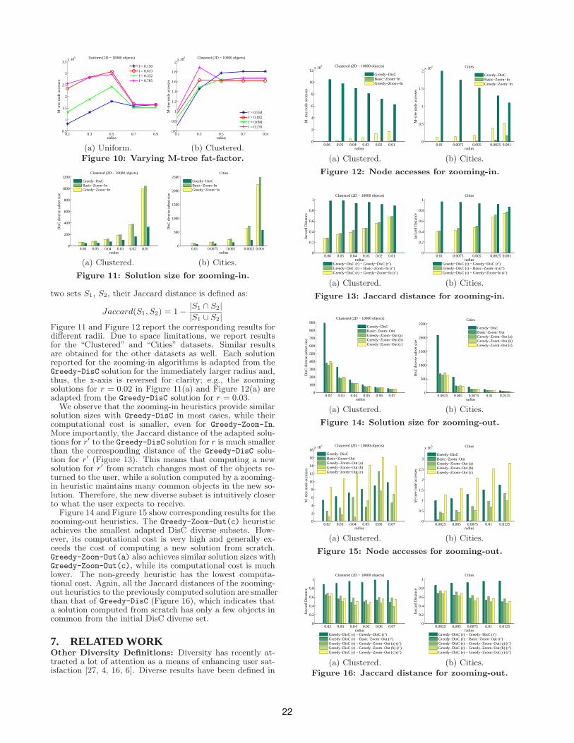
Figure 11 and Figure 12 report the corresponding results fordifferent radii. Due to space limitations, we report resultsfor the “Clustered” and “Cities” datasets. Similar resultsare obtained for the other datasets as well. Each solutionreported for the zooming-in algorithms is adapted from theGreedy-DisC solution for the immediately larger radius and,thus, the x-axis is reversed for clarity; e.g., the zoomingsolutions for r = 0.02 in Figure 11(a) and Figure 12(a) areadapted from the Greedy-DisC solution for r = 0.03.

We observe that the zooming-in heuristics provide similarsolution sizes with Greedy-DisC in most cases, while theircomputational cost is smaller, even for Greedy-Zoom-In.More importantly, the Jaccard distance of the adapted solu-tions for r′ to the Greedy-DisC solution for r is much smallerthan the corresponding distance of the Greedy-DisC solu-tion for r′ (Figure 13). This means that computing a newsolution for r′ from scratch changes most of the objects re-turned to the user, while a solution computed by a zooming-in heuristic maintains many common objects in the new so-lution. Therefore, the new diverse subset is intuitively closerto what the user expects to receive.

Figure 14 and Figure 15 show corresponding results for thezooming-out heuristics. The Greedy-Zoom-Out(c) heuristicachieves the smallest adapted DisC diverse subsets. How-ever, its computational cost is very high and generally ex-ceeds the cost of computing a new solution from scratch.Greedy-Zoom-Out(a) also achieves similar solution sizes withGreedy-Zoom-Out(c), while its computational cost is muchlower. The non-greedy heuristic has the lowest computa-tional cost. Again, all the Jaccard distances of the zooming-out heuristics to the previously computed solution are smallerthan that of Greedy-DisC (Figure 16), which indicates thata solution computed from scratch has only a few objects incommon from the initial DisC diverse set.

7. RELATED WORKOther Diversity Definitions: Diversity has recently at-tracted a lot of attention as a means of enhancing user sat-isfaction [27, 4, 16, 6]. Diverse results have been defined in

0.010.020.030.040.050.060

2

4

6

8

10

12x 10

5 Clustered (2D − 10000 objects)

radius

M−

tree

nod

e ac

cess

es

Greedy−DisCBasic−Zoom−InGreedy−Zoom−In

(a) Clustered.

0.0010.00250.0050.00750.010

0.5

1

1.5

2x 10

5 Cities

radius

M−

tree

nod

e ac

cess

es

Greedy−DisCBasic−Zoom−InGreedy−Zoom−In

(b) Cities.

Figure 12: Node accesses for zooming-in.

0.010.020.030.040.050.060

0.2

0.4

0.6

0.8

1Clustered (2D − 10000 objects)

radius

Jacc

ard

Dis

tanc

e

Greedy−DisC (r) − Greedy−DisC (r’)Greedy−DisC (r) − Basic−Zoom−In (r’)Greedy−DisC (r) − Greedy−Zoom−In (r’)

(a) Clustered.

0.0010.00250.0050.00750.010

0.2

0.4

0.6

0.8

1Cities

radius

Jacc

ard

Dis

tanc

e

Greedy−DisC (r) − Greedy−DisC (r’)Greedy−DisC (r) − Basic−Zoom−In (r’)Greedy−DisC (r) − Greedy−Zoom−In (r’)

(b) Cities.

Figure 13: Jaccard distance for zooming-in.

0.02 0.03 0.04 0.05 0.06 0.070

100

200

300

400

500

600

700

800

900Clustered (2D − 10000 objects)

radius

Dis

C d

iver

se s

ubse

t siz

e

Greedy−DisCBasic−Zoom−OutGreedy−Zoom−Out (a)Greedy−Zoom−Out (b)Greedy−Zoom−Out (c)

(a) Clustered.

0.0025 0.005 0.0075 0.01 0.01250

500

1000

1500

2000

2500Cities

radius

Dis

C d

iver

se s

ubse

t siz

e

Greedy−DisCBasic−Zoom−OutGreedy−Zoom−Out (a)Greedy−Zoom−Out (b)Greedy−Zoom−Out (c)

(b) Cities.

Figure 14: Solution size for zooming-out.

0.02 0.03 0.04 0.05 0.06 0.070

2

4

6

8

10

12

14

16

18x 10

5 Clustered (2D − 10000 objects)

radius

M−

tree

nod

e ac

cess

es

Greedy−DisCBasic−Zoom−OutGreedy−Zoom−Out (a)Greedy−Zoom−Out (b)Greedy−Zoom−Out (c)

(a) Clustered.

0.0025 0.005 0.0075 0.01 0.01250

0.5

1

1.5

2

2.5

3

x 105 Cities

radius

M−

tree

nod

e ac

cess

es

Greedy−DisCBasic−Zoom−OutGreedy−Zoom−Out (a)Greedy−Zoom−Out (b)Greedy−Zoom−Out (c)

(b) Cities.

Figure 15: Node accesses for zooming-out.

0.02 0.03 0.04 0.05 0.06 0.070

0.2

0.4

0.6

0.8

1Clustered (2D − 10000 objects)

radius

Jacc

ard

Dis

tanc

e

Greedy−DisC (r) − Greedy−DisC (r’)Greedy−DisC (r) − Basic−Zoom−Out (r’)Greedy−DisC (r) − Greedy−Zoom−Out (a) (r’)Greedy−DisC (r) − Greedy−Zoom−Out (b) (r’)Greedy−DisC (r) − Greedy−Zoom−Out (c) (r’)

(a) Clustered.

0.0025 0.005 0.0075 0.01 0.01250

0.2

0.4

0.6

0.8

1Cities

radius

Jacc

ard

Dis

tanc

e

Greedy−DisC (r) − Greedy−DisC (r’)Greedy−DisC (r) − Basic−Zoom−Out (r’)Greedy−DisC (r) − Greedy−Zoom−Out (a) (r’)Greedy−DisC (r) − Greedy−Zoom−Out (b) (r’)Greedy−DisC (r) − Greedy−Zoom−Out (c) (r’)

(b) Cities.Figure 16: Jaccard distance for zooming-out.

22

various ways [10], namely in terms of content (or similarity),novelty and semantic coverage. Similarity definitions (e.g.,[31]) interpret diversity as an instance of the p-dispersionproblem [13] whose objective is to choose p out of n givenpoints, so that the minimum distance between any pair ofchosen points is maximized. Our approach differs in thatthe size of the diverse subset is not an input parameter.Most current novelty and semantic coverage approaches todiversification (e.g., [9, 3, 29, 14]) rely on associating a di-versity score with each object in the result and then eitherselecting the top-k highest ranked objects or those objectswhose score is above some threshold. Such diversity scoresare hard to interpret, since they do not depend solely onthe object. Instead, the score of each object is relative towhich objects precede it in the rank. Our approach is fun-damentally different in that we treat the result as a wholeand select DisC diverse subsets of it that fully cover it.

Another related work is that of [18] that extends near-est neighbor search to select k neighbors that are not onlyspatially close to the query object but also differ on a set ofpredefined attributes above a specific threshold. Our work isdifferent since our goal is not to locate the nearest and mostdiverse neighbors of a single object but rather to locate anindependent and covering subset of the whole dataset.

On a related issue, selecting k representative skyline ob-jects is considered in [22]. Representative objects are se-lected so that the distance between a non-selected skylineobject from its nearest selected object is minimized. Finally,another related method for selecting representative results,besides diversity-based ones, is k-medoids, since medoidscan be viewed as representative objects (e.g., [19]). However,medoids may not cover all the available space. Medoids wereextended in [5] to include some sense of relevance (prioritymedoids).

The problem of diversifying continuous data has been re-cently considered in [12, 21, 20] using a number of variationsof the MaxMin and MaxSum diversification models.

Results from Graph Theory: The properties of inde-pendent and dominating (or covering) subsets have beenextensively studied. A number of different variations ex-ist. Among these, the Minimum Independent Dominat-

ing Set Problem (which is equivalent to the r-DisC diverseproblem) has been shown to have some of the strongest neg-ative approximation results: in the general case, it cannotbe approximated in polynomial time within a factor of n1−ǫ

for any ǫ > 0 unless P = NP [17]. However, some approxi-mation results have been found for special graph cases, suchas bounded degree graphs [7]. In our work, rather than pro-viding polynomial approximation bounds for DisC diversity,we focus on the efficient computation of non-minimum butsmall DisC diverse subsets. There is a substantial amountof related work in the field of wireless networks research,since a Minimum Connected Dominating Set of wirelessnodes can be used as a backbone for the entire network [24].Allowing the dominating set to be connected has an impacton the complexity of the problem and allows different algo-rithms to be designed.

8. SUMMARY AND FUTURE WORKIn this paper, we proposed a novel, intuitive definition of

diversity as the problem of selecting a minimum represen-tative subset S of a result P, such that each object in P isrepresented by a similar object in S and that the objectsincluded in S are not similar to each other. Similarity ismodeled by a radius r around each object. We call suchsubsets r-DisC diverse subsets of P. We introduced adap-tive diversification through decreasing r, termed zooming-in,and increasing r, called zooming-out. Since locating min-imum r-DisC diverse subsets is an NP-hard problem, we

introduced heuristics for computing approximate solutions,including incremental ones for zooming, and provided corre-sponding theoretical bounds. We also presented an efficientimplementation based on spatial indexing.

There are many directions for future work. We are cur-rently looking into two different ways of integrating rel-evance with DisC diversity. The first approach is by a“weighted” variation of the DisC subset problem, where eachobject has an associated weight based on its relevance. Nowthe goal is to select a DisC subset having the maximum sumof weights. The other approach is to allow multiple radii,so that relevant objects get a smaller radius than the ra-dius of less relevant ones. Other potential future directionsinclude implementations using different data structures anddesigning algorithms for the online version of the problem.

AcknowledgmentsM. Drosou was supported by the ESF and Greek nationalfunds through the NSRF - Research Funding Program: “Her-aclitus II”. E. Pitoura was supported by the project “Inter-Social” financed by the European Territorial CooperationOperational Program “Greece - Italy” 2007-2013, co-fundedby the ERDF and national funds of Greece and Italy.

9. REFERENCES[1] Acme digital cameras database. http://acme.com/digicams.[2] Greek cities dataset. http://www.rtreeportal.org.[3] R. Agrawal, S. Gollapudi, A. Halverson, and S. Ieong.

Diversifying search results. In WSDM, 2009.[4] A. Angel and N. Koudas. Efficient diversity-aware search.

In SIGMOD, 2011.[5] R. Boim, T. Milo, and S. Novgorodov. Diversification and

refinement in collaborative filtering recommender. InCIKM, 2011.

[6] A. Borodin, H. C. Lee, and Y. Ye. Max-sum diversifcation,monotone submodular functions and dynamic updates. InPODS, 2012.

[7] M. Chlebık and J. Chlebıkova. Approximation hardness ofdominating set problems in bounded degree graphs. Inf.Comput., 206(11), 2008.

[8] B. N. Clark, C. J. Colbourn, and D. S. Johnson. Unit diskgraphs. Discrete Mathematics, 86(1-3), 1990.

[9] C. L. A. Clarke, M. Kolla, G. V. Cormack, O. Vechtomova,A. Ashkan, S. Buttcher, and I. MacKinnon. Novelty anddiversity in information retrieval evaluation. In SIGIR,2008.

[10] M. Drosou and E. Pitoura. Search result diversification.SIGMOD Record, 39(1), 2010.

[11] M. Drosou and E. Pitoura. DisC diversity:Result diversification based on dissimilarity and coverage,Technical Report. University of Ioannina, 2012.

[12] M. Drosou and E. Pitoura. Dynamic diversification ofcontinuous data. In EDBT, 2012.

[13] E. Erkut, Y. Ulkusal, and O. Yenicerioglu. A comparison ofp-dispersion heuristics. Computers & OR, 21(10), 1994.

[14] P. Fraternali, D. Martinenghi, and M. Tagliasacchi. Top-kbounded diversification. In SIGMOD, 2012.

[15] M. R. Garey and D. S. Johnson. Computers andIntractability: A Guide to the Theory of NP-Completeness.W. H. Freeman, 1979.

[16] S. Gollapudi and A. Sharma. An axiomatic approach forresult diversification. In WWW, 2009.

[17] M. M. Halldorsson. Approximating the minimum maximalindependence number. Inf. Process. Lett., 46(4), 1993.

[18] A. Jain, P. Sarda, and J. R. Haritsa. Providing diversity ink-nearest neighbor query results. In PAKDD, 2004.

[19] B. Liu and H. V. Jagadish. Using trees to depict a forest.PVLDB, 2(1), 2009.

[20] E. Minack, W. Siberski, and W. Nejdl. Incrementaldiversification for very large sets: a streaming-basedapproach. In SIGIR, 2011.

[21] D. Panigrahi, A. D. Sarma, G. Aggarwal, and A. Tomkins.Online selection of diverse results. In WSDM, 2012.

[22] Y. Tao, L. Ding, X. Lin, and J. Pei. Distance-basedrepresentative skyline. In ICDE, pages 892–903, 2009.

23

p

p1

p2

a

b

c x

y

z

r

(a)

p1 p2

p3

p

b

ca

d

A

a

r1

r2

(b)

pv5

v4

a

br1

r2

v1

v2

v3

A

(c)

Figure 17: Independent neighbors.

[23] M. T. Thai, F. Wang, D. Liu, S. Zhu, and D.-Z. Du.Connected dominating sets in wireless networks withdifferent transmission ranges. IEEE Trans. Mob. Comput.,6(7), 2007.

[24] M. T. Thai, N. Zhang, R. Tiwari, and X. Xu. Onapproximation algorithms of k-connected m-dominatingsets in disk graphs. Theor. Comput. Sci., 385(1-3), 2007.

[25] C. J. Traina, A. J. M. Traina, C. Faloutsos, and B. Seeger.Fast indexing and visualization of metric data sets usingslim-trees. IEEE Trans. Knowl. Data Eng., 14(2), 2002.

[26] E. Vee, U. Srivastava, J. Shanmugasundaram, P. Bhat, andS. Amer-Yahia. Efficient computation of diverse queryresults. In ICDE, 2008.

[27] M. R. Vieira, H. L. Razente, M. C. N. Barioni,M. Hadjieleftheriou, D. Srivastava, C. Traina, and V. J.Tsotras. On query result diversification. In ICDE, 2011.

[28] K. Xing, W. Cheng, E. K. Park, and S. Rotenstreich.Distributed connected dominating set construction ingeometric k-disk graphs. In ICDCS, 2008.

[29] C. Yu, L. V. S. Lakshmanan, and S. Amer-Yahia. It takesvariety to make a world: diversification in recommendersystems. In EDBT, 2009.

[30] P. Zezula, G. Amato, V. Dohnal, and M. Batko. SimilaritySearch - The Metric Space Approach. Springer, 2006.

[31] M. Zhang and N. Hurley. Avoiding monotony: improvingthe diversity of recommendation lists. In RecSys, 2008.

[32] C.-N. Ziegler, S. M. McNee, J. A. Konstan, and G. Lausen.Improving recommendation lists through topicdiversification. In WWW, 2005.

AppendixProof of Lemma 3: Let p1, p2 be two independent neigh-bors of p. Then, it must hold that ∠p1pp2 (in the Euclideanspace) is larger than π

4. We will prove this using contra-

diction. p1, p2 are neighbors of p so they must reside inthe shaded area of Figure 17(a). Without loss of generality,assume that one of them, say p1, is aligned to the vertical

axis. Assume that ∠p1pp2 ≤ π4. Then cos(∠p1pip2) ≥

√2

2.

It holds that b ≤ r and c ≤ r, thus, using the cosine law weget that a2 ≤ r2(2 −

√2) (1). The Manhattan distance of

p1,p2 is equal to x+ y =√

a2 + 2xy (2). Also, the following

hold: x =√

b2 − z2, y = c − z and z = b cos(∠p1pip2) ≥b√

22

. Substituting z and c in the first two equations, we get

x ≤ b√2

and y ≤ r − b√

22

. From (1),(2) we now get that

x + y ≤ r, which contradicts the independence of p1 and p2.Therefore, p can have at most (2π/π

4) − 1 = 7 independent

neighbors.

Proof of Theorem 2: We consider that inserting a node uinto S has cost 1. We distribute this cost equally among allcovered nodes, i.e., after being labeled grey, nodes are notcharged anymore. Assume an optimal minimum dominatingset S∗. The graph G can be decomposed into a number ofstar-shaped subgraphs, each of which has one node from S∗

at its center. The cost of an optimal minimum dominatingset is exactly 1 for each star-shaped subgraph. We showthat for a non-optimal set S, the cost for each star-shapedsubgraph is at most ln∆, where ∆ is the maximum degreeof the graph. Consider a star-shaped subgraph of S∗ with u

at its center and let NWr (u) be the number of white nodes

in it. If a node in the star is labeled grey by Greedy-C,these nodes are charged some cost. By the greedy conditionof the algorithm, this cost can be at most 1/|NW

r (u)| pernewly covered node. Otherwise, the algorithm would ratherhave chosen u for the dominating set because u would coverat least |NW

r (u)| nodes. In the worst case, no two nodesin the star of u are covered at the same iteration. In thiscase, the first node that is labeled grey is charged at most1/(δ(u)+1), the second node is charged at most 1/δ(u) andso on, where δ(u) is the degree of u. Therefore, the totalcost of a star is at most:

1

δ(u) + 1+

1

δ(u)+. . .+

1

2+1 = H(δ(u)+1) ≤ H(∆+1) ≈ ln ∆

where H(i) is the ith harmonic number. Since a minimumdominating set is equal or smaller than a minimum indepen-dent dominating set, the theorem holds.

Proof of Lemma 4(i): For the proof, we use a techniquefor partitioning the annulus between r1 and r2 similar tothe one in [23] and [28]. Let r1 be the radius of an objectp (Figure 17(b)) and α a real number with 0 < α < π

3.

We draw circles around the object p with radii (2cosα)xp ,(2cosα)xp+1, (2cosα)xp+2, . . . , (2cosα)yp−1, (2cosα)yp , suchthat (2cosα)xp ≤ r1 and (2cosα)xp+1 > r2 and (2cosα)yp−1 <

r2 and (2cosα)yp ≥ r2. It holds that xp =⌊

ln r1

ln(2 cos α)

⌋

and

yp =⌈

ln r2

ln(2 cos α)

⌉

. In this way, the area around p is parti-

tioned into yp − xp annuluses plus the r1-disk around p.Consider an annulus A. Let p1 and p2 be two neighbors

of p in A with dist(p1, p2) > r1. Then, it must hold that∠p1pp2 > α. To see this, we draw two segments from pcrossing the inner and outer circles of A at a, b and c, dsuch that p1 resides in pb and ∠bpd = α, as shown in thefigure. Due to the construction of the circles, it holds that|pb||pc| = |pd|

|pa| = 2 cos α. From the cosine law for p△ad, we get

that |ad| = |pa| and, therefore, it holds that |cb| = |ad| =|pa| = |pc|. Therefore, for any object p3 in the area abcd ofA, it holds that |pp3| > |bp3| which means that all objects inthat area are neighbors of p1, i.e., at distance less or equalto r1. For this reason, p2 must reside outside this area whichmeans that ∠p1pp2 > α. Based on this, we see that thereexist at most 2π

α− 1 independent (for r1) nodes in A.

The same holds for all annuluses. Therefore, we have atmost (yp−xp)

(

2πα

− 1)

independent nodes in the annuluses.For 0 < α < π

3, this has a minimum when α is close to π

5and

that minimum value is 9⌈

ln(r2/r1)ln(2 cos(π/5))

⌉

= 9⌈

logβ(r2/r1)⌉

,

where β = 1+√

52

.

Proof of Lemma 4(ii): Let r1 be the radius of an object p.We draw Manhattan circles around the object p with radiir1, 2r1, . . . until the radius r2 is reached. In this way, the

area around p is partitioned into γ =⌈

r2−r1

r1

⌉

Manhattan

annuluses plus the r1-Manhattan-disk around p.Consider an annulus A. The objects shown in Figure 17(c)

cover the whole annulus and their Manhattan pairwise dis-tances are all greater or equal to r1. Assume that the annu-lus spans among distance ir1 and (i+1)r1 from p, where i is

an integer with i > 1. Then, |ab| =√

2 (ir1 + r1/2)2. Also,

for two objects p1, p2 it holds that |p1p2| =√

2 (r1/2)2.

Therefore, at one quadrant of the annulus there are |ab||p1p2|

= 2i + 1 independent neighbors which means that there are4(2i + 1) independent neighbors in A. Therefore, there arein total

∑γi=1 4(2i+1) independent (for r1) neighbors of p.

24