DISADVANTAGES OF STATISTICAL COMPARISON …bioma.ijs.si/proceedings/2016/07 - Disadvantages of...

DISADVANTAGES OF STATISTICALCOMPARISON OF STOCHASTICOPTIMIZATION ALGORITHMS

Tome EftimovComputer Systems Department, Jozef Stefan Institute, Ljubljana, Slovenia

Jozef Stefan International Postgraduate School, Ljubljana, Slovenia

[email protected]

Peter KorosecComputer Systems Department, Jozef Stefan Institute, Ljubljana, Slovenia

[email protected]

Barbara Korousic SeljakComputer Systems Department, Jozef Stefan Institute, Ljubljana, Slovenia

Jozef Stefan International Postgraduate School, Ljubljana, Slovenia

[email protected]

Abstract In this paper a short overview and a case study in a statistical compari-son of stochastic optimization algorithms are presented. The algorithmsare part of the Black-Box Optimization Benchmarking 2015 competi-tion that was held at the 5th GECCO Workshop for Real-ParameterOptimization. The question about the difference between parametricand non-parametric tests for single-problem analysis and for multiple-problem analysis is addressed in this paper. The main contributions arethe disadvantages that can appear by using multiple-problem analysis,in the case when the data of some algorithms includes outliers.

Keywords: Comparative study, Non-parametric tests, Parametric tests, Statisticalmethods, Stochastic optimization algorithms.

1. Introduction

Over the last years, many machine learning and stochastic optimiza-tion algorithms have been developed. For each new algorithm, according

105

106 BIOINSPIRED OPTIMIZATION METHODS AND THEIR APPLICATIONS

to its performance, we need to decide whether it is better than the com-pared algorithms used on the same problem.

One of the most common ways to compare algorithms used on thesame problem is to use statistical tests as comparison techniques of theirperformance [4, 5, 6, 9, 10]. The common thing of the comparativestudies, independently of the research area (machine learning, stochasticoptimization or some other research areas), is that they are based on theidea of hypothesis testing [18].

The hypothesis testing, also called significance testing, is a method ofstatistical inference that could be used for testing a hypothesis about pa-rameter in a population, using data measured in a data sample, or aboutthe relationship between two or more populations, using data measuredin data samples. The method starts by defining two hypotheses, the nullhypothesis H0 and the alternative hypothesis HA. The null hypothesisis a statement that there is no difference or no effect and the alternativehypothesis is a statement that directly contradicts the null hypothesisby indicating the presence of a difference or an effect. This step in thehypothesis testing is very important, because mis-stating the hypothe-ses will disrupt the rest of the process. The second step is to select anappropriate test statistic T , which is a mathematical formula that al-lows researchers to determine the likelihood of obtaining the outcomesif the null hypothesis is true. Then, the level of significance α, alsocalled significance level, which is the probability threshold below whichthe null hypothesis will be rejected, needs to be selected. The last stepof the hypothesis testing is to make a decision either to reject the nullhypothesis in favor of the alternative or not to reject it. The last stepcan be done with two different approaches. In the standard approach,the possible values of the test statistic for which the null hypothesis isrejected, also called the critical region, are calculated using the distribu-tion of the test statistic and the probability of the critical region that isthe level of significance α. Then the observed value of the test statisticTobs is calculated according to the observations from the data sample. Ifthe observed value of the test statistic is in the critical region, the nullhypothesis is rejected, and if not, it fails to reject the null hypothesis.In the alternative approach, instead of defining the critical region, a p-value that is the probability of obtaining the sample outcome, given thenull hypothesis is true, is calculated. The null hypothesis is rejected, ifthe p-value is less than the selected significance level (the most commonvalues for it are 0.05 and 0.01), and if not, it fails to reject the nullhypothesis.

In this paper we follow the recommendations given in some papers[4, 5, 6, 9, 10] in order to perform correct statistical comparison of

Disadvantages of Statistical Comparison of Stochastic Optimization . . . 107

the behavior of some of the stochastic optimization algorithms overoptimization problems presented of the Black-Box Benchmarking 2015(BBOB 2015) competition helded at the 5th GECCO Workshop onReal-Parameter Optimization organized at the Genetic and Evolution-ary Computation Conference (GECCO 2015) [1].

This paper can be seen as a tutorial and a case study on the use ofstatistical tests for comparison of stochastic optimization algorithms. InSection 2 we give a review and important comments with regard to thestandard statistical tests, the parametric tests, and the non-parametrictests. Section 3 presents the empirical study carried out on the resultsfrom the workshop in different scenarios, using pairwise comparison forsingle-problem analysis, pairwise comparison for multiple-problem anal-ysis, multiple comparisons for single-problem analysis, and multiple com-parisons for multiple-problem analysis. In Section 4 we conclude thepaper by discussing the disadvantages of the standard statistical teststhat are used for statistical comparisons of the behavior of stochasticoptimization algorithms.

2. Parametric Versus Non-parametric StatisticalTests

In order to distinguish what to use for your data, between the para-metric and the non-parametric test, the first step is to check the assump-tions of the parametric tests, also called required conditions for the safeuse of parametric tests. So the first step is to use the methods for check-ing the validity of these required conditions. If the data does not satisfythe required conditions for the safe use of parametric tests, then the testscould lead to incorrect conclusions, and it is better to use the analogousnon-parametric test. In general, a non-parametric test is less restrictivethan a parametric one, but it is less powerful than a parametric one,when the required conditions for the safe use of the parametric test aretrue [10].

2.1 Required Conditions for the Safe Use ofParametric Tests

The assumptions or the required conditions for the safe use of para-metric tests are the independence, the normality, and the homoscedas-ticity of the variances of the data.

Two events, A and B are independent, if the fact that A occurs doesnot affect the probability of B occurring. When we compare the behaviorof the stochastic optimization algorithms, they are usually independent.


The assumption of normality is just a hypothesis that a random vari-able of interest, or in our case the data from the data sample, is dis-tributed according to the normal or Gaussian distribution with mean µand standard deviation σ. In order to check the validity of this con-dition, the recommended statistical tests are Kolmogorov-Smirnov [19],Shapiro-Wilk [23], and D’Agostino-Pearson [3]. The validity of this con-dition can be also checked by using graphical representation of the datausing histograms and qunatile-quantile plots (Q-Q plots) [7].

The homoscedasticity indicates the hypothesis of equality of variances,and the Levene’s test is used to check the validity of this condition [13].Using this test we can see whether or not a given number of sampleshave equal variances or not.

2.2 An Overview of Some Standard Statistical Tests

In Table 1 we give an overview of the most commonly used statisticaltests that can be used for statistical comparison between two or multiplealgorithms. We do not go into details for each of them, because theyare standard statistical tests [18]. Which of them is chosen dependson the type of analysis we want to perform, either single-problem ormultiple-problem analysis.

Table 1: An overview of parametric and non-parametric tests

Two Algorithms Multiple Algorithms

Parametric tests Paired T-Test Repeated-Measures ANOVA

Non-parametric testsWilcoxon Signed-Rank Test,

The Sign TestFriedman Test,

Iman-Davenport Test

The single-problem analysis is the scenario when the data comes frommultiple runs of the stochastic optimization algorithms on one problem,one function. This scenario is common in stochastic optimization al-gorithms, since they are of stochastic nature, meaning we do not haveany guaranty that the result will be optimal for every run. Moreover,typically even the path leading to the final solution is often different. Soto test the quality of the algorithm, it is not enough to performed justone run, but many of them from which we can draw some conclusions.

The second scenario or the multiple-problem analysis is the scenariowhen several stochastic optimization algorithms are compared on multi-ple problems, multiple functions. In this case, in most papers the authorsuse the averaged results for each function to compose a sample of resultsfor each algorithm.


3. Case Study: Black-Box OptimizationBenchmarking 2015

In order to go through the recommendations of how to perform sta-tistical comparisons of stochastic optimization algorithms and to see thepossible problems that appear, the results from the Black-Box Bench-marking 2015 [1] are used. The Black-Box Benchmarking 2015 is acompetition that provides single-objective functions for benchmarking.In addition, it enables analyses of the performance of the competingalgorithms, and makes it understandable what are the advantages anddisadvantages for each algorithm.

From the competition the algorithms BSif, BSifeg, BSrr, and Srr areused for statistical comparisons. The capital letters, S or BS, denoteSTEP or Brent-STEP method, respectively. The lowercase letters de-note the dimension selection strategy: “rr” for round-robin, “if” for theEWMA estimate of the improvement frequency, and “ifeg” for “if” com-bined with ε-greedy strategy [21]. For each of them the results for 24different noiseless test functions in 5 dimensionality (2, 3, 5, 10, and20) are selected. At the end, the statistical comparison is performedby comparing the algorithms on 22 different noiseless functions becausesome of them do not provide data for two functions of the benchmarkwhen the dimension is 20.

The test functions are from 5 groups: separable functions, functionswith low or moderate conditioning, function with hight conditioning andunimodal, multi-modal functions with adequate global structure, andmulti-modal functions with week global structure. More details aboutthem can be found in [15].

We have done the statistical comparisons in “R programming lan-guage”, by using the “lawstat” package [11] for the Levene’s Test, the“stats” package [22] for the Kolmogorov-Smirnov Test, the Paired-T Test[16], the Shapiro-Wilk Test, and the Wilcoxon Signed-Rank Test [17], andthe “scmap” package [2] for the Iman-Davenport Test [6], the FriedmanTest [6], and the Friedman Algined-Rank Test [6].

3.1 Pairwise and Multiple Comparisons forSingle-Problem Analysis

In this section pairwise comparison for single-problem analysis is pre-sented together with comments for multiple comparisons for single-problemanalysis. The BSif and BSifeg algorithms are the two algorithms usedfor pairwise comparison. The pairwise comparisons between these twoalgorithms for single-problem analysis are performed on 22 benchmarkfunctions when the dimension is 10.


At the beginning of each statistical comparison, the required condi-tions for the safe use of the parametric tests are checked.

In case of the single-problem analysis the multiple runs of the algo-rithm on the same function are independent.

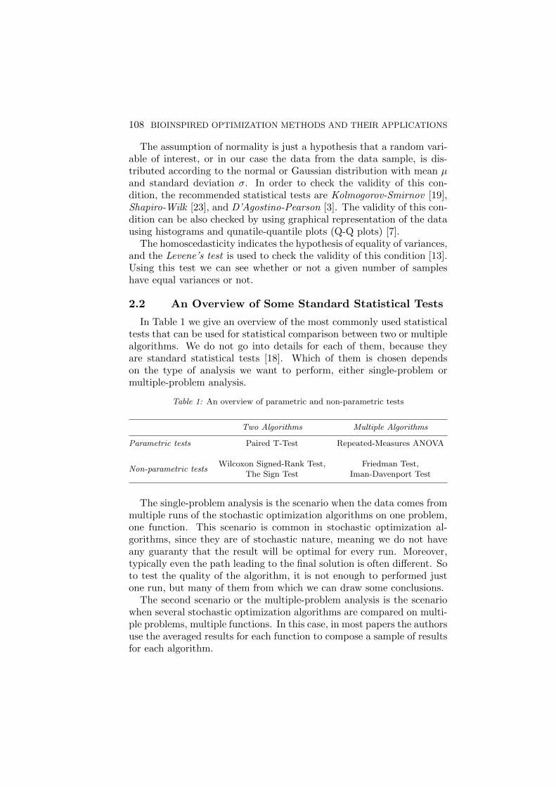
To check for normality, the Shapiro-Wilk Test and graphical represen-tations by representing the data using histograms and quantile-quantileplots are used. The p-values from the Shapiro-Wilk Test are presentedin the Table 2, and when the p-value is smaller than the significancelevel (we used 0.05), then the null hypothesis is rejected, and we assumethe data is not normally distributed.

Table 2: Test of normality using Shapiro-Wilk Test

f1 f2 f3 f4 f5 f6 f7 f8

p-value BSif - (.61) ∗(.00) (.70) ∗(.01) ∗(.02) ∗(.01) (.05)p-value BSifeg - ∗(.03) ∗(.00) (.47) ∗(.01) ∗(.00) (.28) ∗(.00)

f9 f10 f11 f12 f13 f14 f15 f16

p-value BSif∗(.00) ∗(.00) (.49) (.23) ∗(.01) ∗(.00) ∗(.02) (.05)

p-value BSifeg∗(.00) ∗(.01) (.28) ∗(.00) ∗(.00) ∗(.00) ∗(.02) (.24)

f17 f18 f19 f20 f21 f22

p-value BSif (.21) ∗(.04) (.16) ∗(.01) ∗(.00) ∗(.00)p-value BSifeg (.24) (.13) (.07) (.10) ∗(.00) ∗(.00)

∗ indicates that the normality condition is not satisfied.

From the same table we can see that there are 6 cases in which thedata from both algorithms comes from normal distribution (f1, f4, f11,f16, f17, f19), 6 cases in which the data only from one of the algorithmscomes from normal distribution (f2, f7, f8, f12, f18, f20), and 10 casesin which the data from both algorithms is not normally distributed (f3,f5, f6, f9, f10, f13,f14, f15, f21, f22).

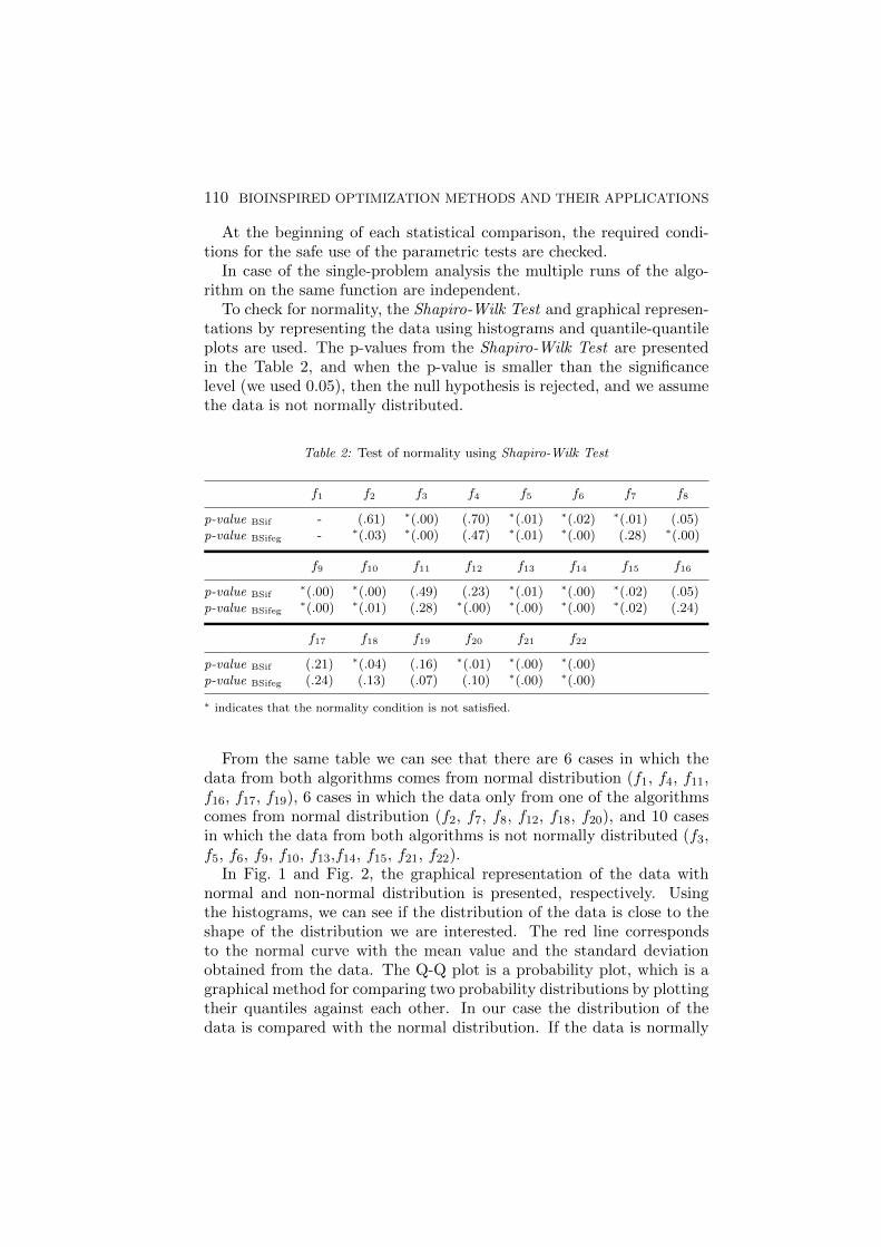
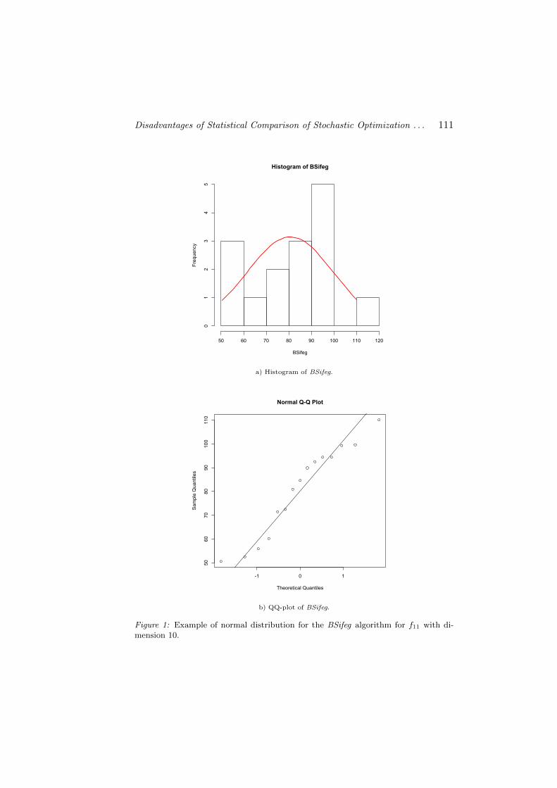
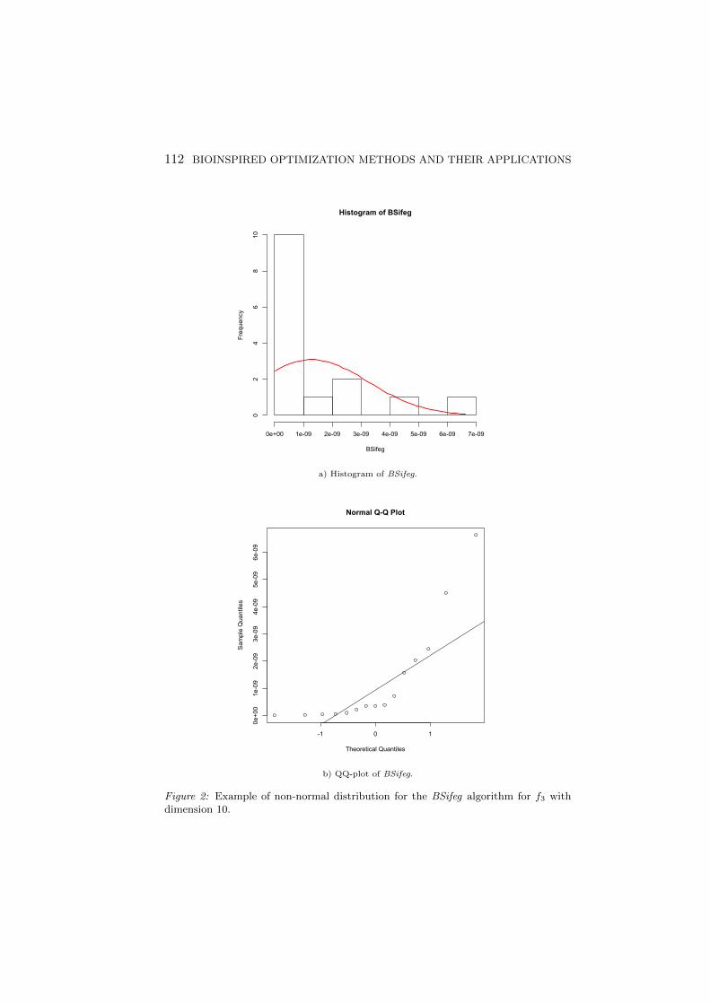
In Fig. 1 and Fig. 2, the graphical representation of the data withnormal and non-normal distribution is presented, respectively. Usingthe histograms, we can see if the distribution of the data is close to theshape of the distribution we are interested. The red line correspondsto the normal curve with the mean value and the standard deviationobtained from the data. The Q-Q plot is a probability plot, which is agraphical method for comparing two probability distributions by plottingtheir quantiles against each other. In our case the distribution of thedata is compared with the normal distribution. If the data is normally


Histogram of BSifeg

BSifeg

Frequency

50 60 70 80 90 100 110 120

01

23

45

a) Histogram of BSifeg.

-1 0 1

5060

7080

90100

110

Normal Q-Q Plot

Theoretical Quantiles

Sam

ple

Qua

ntile

s

b) QQ-plot of BSifeg.

Figure 1: Example of normal distribution for the BSifeg algorithm for f11 with di-mension 10.


Histogram of BSifeg

BSifeg

Frequency

0e+00 1e-09 2e-09 3e-09 4e-09 5e-09 6e-09 7e-09

02

46

810

a) Histogram of BSifeg.

-1 0 1

0e+00

1e-09

2e-09

3e-09

4e-09

5e-09

6e-09

Normal Q-Q Plot

Theoretical Quantiles

Sam

ple

Qua

ntile

s

b) QQ-plot of BSifeg.

Figure 2: Example of non-normal distribution for the BSifeg algorithm for f3 withdimension 10.


distributed, the data points in the Q-Q normal plot can be approximatedwith a straight diagonal line.

The next step of the analysis is to check the homoscedasticity. InTable 3 the p-values from the Levene’s Test for checking homoscedastic-ity, based on means, are presented. When the p-value obtained by thistest is smaller than the significance level (we used 0.05), then the nullhypothesis is rejected, and this indicates the existence of a violation ofthe hypothesis of equality of variances.

Table 3: Test of homoscedasticity using the Levene’s Test

f1 f2 f3 f4 f5 f6 f7 f8 f9

p-value - (.08) (.98) (.99) 1 (.05) (.57) (.07) ∗(.01)

f10 f11 f12 f13 f14 f15 f16 f17 f18

p-value (.97) (.37) ∗(.00) ∗(.00) ∗(.04) (.26) (.27) (.85) (.29)

f19 f20 f21 f22

p-value (.77) (.94) (.41) (.66)

∗ indicates that the homoscedasticity condition is not satisfied.

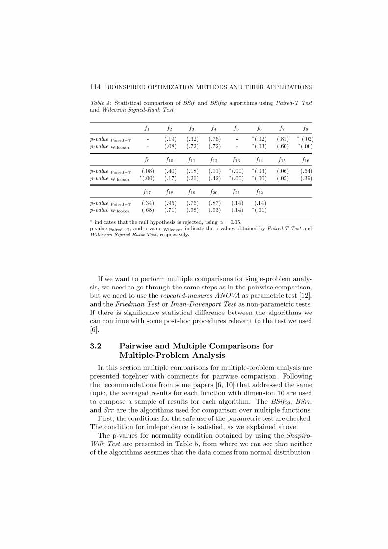
After checking the required conditions for the safe use of the para-metric tests, the pairwise comparison of these two algorithms on eachfunction separately is performed using the Paired-T Test as parametrictest and the Wilcoxon Signed-Rank Test as non-parametric test. The p-values obtained by these two tests for the pairwise comparison of the twoalgorithms are presented in Table 4, where the p-value smaller than thesignificance level of 0.05, indicates that there is a significant statisticaldifference between the performance of the two algorithms.

From the Table 4 we can see that for functions f9 and f22 we obtaineddifferent results according to the Paired-T Test and the Wilcoxon Signed-Rank Test. In order to select the true result, first we need to check theresults for the validity of the required conditions for the safe use of para-metric tests. If we look at Table 2, we can see that for these two functionsthe normality condition is not satisfied, so we can not use the parametrictests because they could lead to incorrect conclusions, and we need toconsider the result obtained by the Wilcoxon Signed-Rank Test. Usingthis test in the case of both functions the null hypothesis is rejected usinga significance level of 0.05, so there is a significant statistical differencebetween the performance of the two algorithms, BSif and BSifeg, overfunctions, f9 and f22.


Table 4: Statistical comparison of BSif and BSifeg algorithms using Paired-T Testand Wilcoxon Signed-Rank Test

f1 f2 f3 f4 f5 f6 f7 f8

p-value Paired−T - (.19) (.32) (.76) - ∗(.02) (.81) ∗ (.02)p-value Wilcoxon - (.08) (.72) (.72) - ∗(.03) (.60) ∗(.00)

f9 f10 f11 f12 f13 f14 f15 f16

p-value Paired−T (.08) (.40) (.18) (.11) ∗(.00) ∗(.03) (.06) (.64)p-value Wilcoxon

∗(.00) (.17) (.26) (.42) ∗(.00) ∗(.00) (.05) (.39)

f17 f18 f19 f20 f21 f22

p-value Paired−T (.34) (.95) (.76) (.87) (.14) (.14)p-value Wilcoxon (.68) (.71) (.98) (.93) (.14) ∗(.01)

∗ indicates that the null hypothesis is rejected, using α = 0.05.p-value Paired−T, and p-value Wilcoxon indicate the p-values obtained by Paired-T Test andWilcoxon Signed-Rank Test, respectively.

If we want to perform multiple comparisons for single-problem analy-sis, we need to go through the same steps as in the pairwise comparison,but we need to use the repeated-masures ANOVA as parametric test [12],and the Friedman Test or Iman-Davenport Test as non-parametric tests.If there is significance statistical difference between the algorithms wecan continue with some post-hoc procedures relevant to the test we used[6].

3.2 Pairwise and Multiple Comparisons forMultiple-Problem Analysis

In this section multiple comparisons for multiple-problem analysis arepresented togehter with comments for pairwise comparison. Followingthe recommendations from some papers [6, 10] that addressed the sametopic, the averaged results for each function with dimension 10 are usedto compose a sample of results for each algorithm. The BSifeg, BSrr,and Srr are the algorithms used for comparison over multiple functions.

First, the conditions for the safe use of the parametric test are checked.The condition for independence is satisfied, as we explained above.

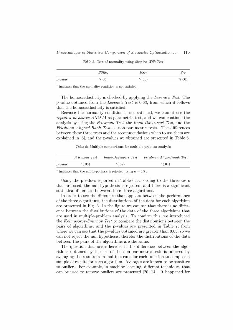
The p-values for normality condition obtained by using the Shapiro-Wilk Test are presented in Table 5, from where we can see that neitherof the algorithms assumes that the data comes from normal distribution.


Table 5: Test of normality using Shapiro-Wilk Test

BSifeg BSrr Srr

p-value ∗(.00) ∗(.00) ∗(.00)

∗ indicates that the normality condition is not satisfied.

The homoscedasticity is checked by applying the Levene’s Test. Thep-value obtained from the Levene’s Test is 0.63, from which it followsthat the homoscedasticity is satisfied.

Because the normality condition is not satisfied, we cannot use therepeated-measures ANOVA as parametric test, and we can continue theanalysis by using the Friedman Test, the Iman-Davenport Test, and theFriedman Aligned-Rank Test as non-parametric tests. The differencesbetween these three tests and the recommendations when to use them areexplained in [6], and the p-values we obtained are presented in Table 6.

Table 6: Multiple comparisons for multiple-problem analysis

Friedman Test Iman-Davenport Test Friedman Aligned-rank Test

p-value ∗(.03) ∗(.02) ∗(.04)

∗ indicates that the null hypothesis is rejected, using α = 0.5 .

Using the p-values reported in Table 6, according to the three teststhat are used, the null hypothesis is rejected, and there is a significantstatistical difference between these three algorithms.

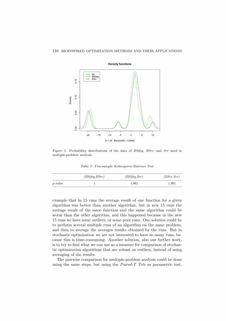
In order to see the difference that appears between the performanceof the three algorithms, the distributions of the data for each algorithmare presented in Fig. 3. In the figure we can see that there is no differ-ence between the distributions of the data of the three algorithms thatare used in multiple-problem analysis. To confirm this, we introducedthe Kolmogorov-Smirnov Test to compare the distributions between thepairs of algorithms, and the p-values are presented in Table 7, fromwhere we can see that the p-values obtained are greater than 0.05, so wecan not reject the null hypothesis, therefor the distributions of the databetween the pairs of the algorithms are the same.

The question that arises here is, if this difference between the algo-rithms obtained by the use of the non-parametric tests is inforced byaveraging the results from multiple runs for each function to compose asample of results for each algorithm. Averages are known to be sensitiveto outliers. For example, in machine learning, different techniques thatcan be used to remove outliers are presented [20, 14]. It happened for


-20 -15 -10 -5 0 5 10

0.00

0.05

0.10

0.15

Density functions

N = 20 Bandwidth = 0.8948

Density

SrrBSifegBSrr

Figure 3: Probability distributions of the data of BSifeg, BSrr, and Srr used inmultiple-problem analysis.

Table 7: Two-sample Kolmogorov-Smirnov Test

(BSifeg,BSrr) (BSifeg,Srr) (BSrr,Srr)

p-value 1 (.86) (.99)

example that in 15 runs the average result of one function for a givenalgorithm was better than another algorithm, but in new 15 runs theaverage result of the same function and the same algorithm could beworse than the other algorithm, and this happened because in the new15 runs we have some outliers, or some poor runs. One solution could beto perform several multiple runs of an algorithm on the same problem,and then to average the averages results obtained by the runs. But instochastic optimization we are not interested to have so many runs, be-cause this is time-consuming. Another solution, also our further work,is to try to find what we can use as a measure for comparison of stochas-tic optimization algorithms that are robust on outliers, instead of usingaveraging of the results.

The pairwise comparison for multiple-problem analysis could be doneusing the same steps, but using the Paired-T Tets as parametric test,


and the Wicoxon Signed-Rank Test or the The Sign Test [8] as non-parametric tests.

4. Conclusion

In this paper a tutorial and a case study of statistical comparison be-tween the behaviour of stochastic optimization algorithms are presented.

The main conclusion of the paper are the disadvantages that can ap-pear in the multiple-problem analysis following the recommendations ofother tutorials that address this topic. These disadvantages can happenby averaging the results from multiple runs for each function to composea sample of results for each algorithm, in the case when the data includesoutliers. In general, the outliers can be skipped using some techniques,but they need to be used with great care. But for multiple-problemanalysis skipping outliers is really a question because only the resultsfor certain problems would be changed and not for other problems. Allthis leads to a need of some new measures that will be robust to outliersand can be used to compose a sample for each algorithm over multipleproblems, and after that to continue the analysis by using some standardstatistical tests.

References

[1] Black-box benchmarking 2015. http://coco.gforge.inria.fr/doku.php?id=

bbob-2015, accessed: 2016-02-01.

[2] B. Calvo and G. Santafe. scmamp: Statistical comparison of multiple algorithmsin multiple problems. The R Journal, 2015.

[3] R. B. D’agostino, A. Belanger, and R. B. D’Agostino Jr. A suggestion for us-ing powerful and informative tests of normality. The American Statistician,44(4):316–321, 1990.

[4] J. Demsar. Statistical comparisons of classifiers over multiple data sets. TheJournal of Machine Learning Research, 7:1–30, 2006.

[5] J. Derrac, S. Garcıa, S. Hui, P. N. Suganthan, and F. Herrera. Analyzing con-vergence performance of evolutionary algorithms: a statistical approach. Infor-mation Sciences, 289:41–58, 2014.

[6] J. Derrac, S. Garcıa, D. Molina, and F. Herrera. A practical tutorial on the use ofnonparametric statistical tests as a methodology for comparing evolutionary andswarm intelligence algorithms. Swarm and Evolutionary Computation, 1(1):3–18, 2011.

[7] J. Devore. Probability and Statistics for Engineering and the Sciences. CengageLearning, 2015.

[8] W. J. Dixon and A. M. Mood. The statistical sign test. Journal of the AmericanStatistical Association, 41(236):557–566, 1946.

[9] S. Garcıa, A. Fernandez, J. Luengo, and F. Herrera. Advanced nonparametrictests for multiple comparisons in the design of experiments in computational


intelligence and data mining: Experimental analysis of power. Information Sci-ences, 180(10):2044–2064, 2010.

[10] S. Garcıa, D. Molina, M. Lozano, and F. Herrera. A study on the use of non-parametric tests for analyzing the evolutionary algorithms behaviour: a casestudy on the CEC2005 special session on real parameter optimization. Journalof Heuristics, 15(6):617–644, 2009.

[11] J. L. Gastwirth, Y. R. Gel, W. L. Wallace Hui, V. Lyubchich, W. Miao,and K. Noguchi. lawstat: Tools for Biostatistics, Public Policy, and Law,2015, r package version 3.0. [Online]. Available: https://CRAN.R-project.org/package=lawstat.

[12] E. R. Girden. ANOVA: Repeated measures. Sage, 1992.

[13] G. V. Glass. Testing homogeneity of variances. American Educational ResearchJournal, 3(3):187–190, 1966.

[14] J. Han, M. Kamber, and J. Pei. Data mining: concepts and techniques. Elsevier,2011.

[15] N. Hansen, A. Auger, S. Finck, and R. Ros. Real-parameter black-box opti-mization benchmarking 2010: Experimental setup. Research Report RR-7215,INRIA, 2010.

[16] H. Hsu and P. A. Lachenbruch. Paired t test. In Wiley Encyclopedia of ClinicalTrials, 2008.

[17] F. Lam and M. Longnecker. A modified wilcoxon rank sum test for paired data.Biometrika, 70(2):510–513, 1983.

[18] E. L. Lehmann, J. P. Romano, and G. Casella. Testing statistical hypotheses.Wiley, New York, 1986.

[19] H. W. Lilliefors. On the kolmogorov-smirnov test for normality with mean andvariance unknown. Journal of the American Statistical Association, 62(318):399–402, 1967.

[20] M. Nikolova. A variational approach to remove outliers and impulse noise. Jour-nal of Mathematical Imaging and Vision, 20(1-2):99–120, 2004.

[21] P. Posık and P. Baudis. Dimension selection in axis-parallel brent-step methodfor black-box optimization of separable continuous functions. Proceedings of theCompanion Publication of the 2015 on Genetic and Evolutionary ComputationConference, pages 1151–1158, 2015.

[22] R Core Team. R: A Language and Environment for Statistical Computing. RFoundation for Statistical Computing, Vienna, Austria, 2015. [Online]. Avail-able: https://www.R-project.org/.

[23] S. S. Shapiro and R. Francia. An approximate analysis of variance test for nor-mality. Journal of the American Statistical Association, 67(337):215–216, 1972.

DISADVANTAGES OF STATISTICAL COMPARISON …bioma.ijs.si/proceedings/2016/07 - Disadvantages of...

Documents

Transcript of DISADVANTAGES OF STATISTICAL COMPARISON …bioma.ijs.si/proceedings/2016/07 - Disadvantages of...