Directional leakage and parameter driftoodgeroo.ucsd.edu/~bob/docs/P79_Morten_IJACSP_draft.pdf ·...

Directional leakage and parameter drift

M. Hovd∗1 and R. R. Bitmead2

1 Engineering Cybernetics Department,Norwegian University of Technology and Science,

Trondheim, Norway.2 Department of Mechanical and Aerospace Engineering,

University of California San Diego,La Jolla, California, USA

SUMMARY

A new method for eliminating parameter drift in parameter estimation problems is proposed. Existing

methods for eliminating parameter drift work either on a limited time horizon, restricts the parameter

estimates to a range that has to be determined a priori, or introduces bias in the parameter estimates

which will degrade steady state performance. The idea of the new method is to apply leakage only

in the directions in parameter space in which the exciting signal is not informative. This avoids the

problem of parameter bias associated with conventional leakage.

key words: Parameter estimation; parameter drift; leakage

1. INTRODUCTION

The problem of parameter drift instability in adaptive systems appears to be pointed out first

by Egardt [1]. Following Egardt, a number of publications deal with classification of different

mechanisms for adaptive control performance problems. Ioannou and Kokotovic [2] identify

different instability mechanisms, and possible ways to amend the resulting poor performance.

∗Correspondence to: Engineering Cybernetics Department, NTNU, N-7491 Trondheim, Norway.This is a modified version of a paper presented at the IFAC Conference DYCOPS 7, Boston, MA, July 2004

Received January 25, 2005

Revised May 30, 2005

2 M. HOVD AND R. R. BITMEAD

Within this set of questions, the present work deals with disturbance-driven parameter drift,

not necessarily in a feedback situation. Other causes for instability include parasitic unmodelled

dynamics, failure of Strictly Positive Real conditions of error systems [3], and unbounded

gains. This latter cause is related to parameter drift, as it occurs when parameters drift to an

uncontrollable model.

There is a substantial literature on parameter drift and avoidance of bursting. Anderson [4]

provide clear analysis of causes for bursting in the absence of persistent excitation, backed by

simple illustrative examples. Common modifications are the use of a deadzone in the parameter

update [1], or the use of leakage [5]. With a deadzone, the parameter updates are stopped as

long as the model follows the observed system behaviour with reasonable accuracy. This will

reduce the parameter drift, which can only occur when the parameter update is active, but

will also reduce the accuracy with which the observed system behaviour can be approximated

by the model.

With leakage, on the other hand, one adds an extra term in the parameter update law

which drives the parameters towards a particular choice of reference values. Sufficiently strong

leakage can eliminate parameter drift, but will bias the parameter values, toward the chosen

reference values. A good portion of luck is required for the reference values for the parameters

to accurately describe the observed input-output behaviour of the system, and hence leakage

typically degrades steady state performance. Sethares et al. [6] study bursting and leakage in

adaptive echo cancellation in telephone lines.

In this work, the properties of the exciting signal and the structure of the model is used

such that the leakage is applied only in the directions in parameter space in which the input-

output data is not informative. Hence, steady state performance is not degraded by the applied

leakage.

The most thorough paper which links strongly to our work in framework and analysis is

Sethares et al. [7]. Here the proposition of excitation subspaces is brooked and analyzed,

Int. J. Adapt. Control Signal Process. 20; :–

Prepared using acsauth.cls

DIRECTIONAL LEAKAGE AND PARAMETER DRIFT 3

with division into excited, unexcited, diminishing-excitation and otherwise-excited orthogonal

subspaces based on the properties of the regressor vectors in a stationary context. The

parameter drift is the unbounded excursion of the parameter error without attendant excursion

of the prediction error. This is driven by an additive disturbance process, which might itself be

decaying to zero. The division into subspaces is analyzed (applicable at least in a stationary

signal environment) and the effect of leakage is studied. Indeed, the prospect of directional

leakage is first countenanced here, without being followed through.

A key tool for the analysis of the stability or otherwise of the adaptive system is averaging,

this tool is used here in much the same way as by Bitmead and Johnson [8]. Another important

tool is bifurcation analysis, which appears to have been most formally applied to bursting in

adaptive feedback in Rey et al. [9].

In the light of these earlier results, our contribution is to formulate directional leakage for

gradient and least-squares algorithms and to explore the consequences of applying a threshold

to the minimal acceptable excitation for preservation of parameter update. The results are

most easily interpreted as building on those of [7] but obviate the need to treat diminishing

excitation or otherwise-excited subspace. An example from adaptive control is evaluated to

illustrated the power of the technique. What we do not consider (other than by example) is

the dependence of excitation subspaces on feedback and the corresponding time-variation, nor

do we treat failure of SPR conditions and parasitics. These would require much more powerful

nonlinear tools, which are difficult to wield.

1.1. Preliminaries

This section defines notation and states some established results on parameter estimation.

Much of the material in this section is extracted from [10], where a more comprehensive

treatment of parameter estimation and adaptive control can be found. We consider the

estimation of model parameters for linear, time-invariant plants. The plant model is expressed




as an nth-order difference equation given by

yk+n + an−1yk+n−1 + · · ·+ a0yk = bn−1un−1 + bn−2un−2 + · · ·+ b0u (1)

Obviously, this corresponds to the discrete transfer function representation

y(z) =bn−1z

n−1 + bn−2zn−2 + · · ·+ b0

zn + an−1zn−1 + zn−2zn−2 + · · ·+ a0u(z) = g(z)u(z) (2)

The unknown parameters are lumped in a parameter vector

θ = [b0, b1, · · · , bn−1, a0, a1, · · · , an−1]T (3)

and all input-output signals are collected in the signal vector

φk−1 = [uk−n, uk−n+1, · · · , uk−1,−yk−n,−yk−n+1, · · · ,−yk−1]T (4)

Thus,(1) can be compactly expressed as

yk = φTk−1θ (5)

In a practical situation, measurements will be corrupted by noise. Therefore it is

commonplace to filter both yk and φk−1 in the equation above with a common low pass

filter. However, in order to keep the presentation simple, we will ignore such filtering in most

of the analysis to follow.

Let θ denote an estimate of the parameter vector θ, and θ = θ− θ denote the corresponding

parameter error vector. The observed model error is denoted e, and is given by

ek = yk − φTk−1θk−1 = θT

k−1φk−1 (6)

1.2. The gradient method

We choose an instantaneous optimization criterion of the form

J(θk) =12(yk − φT

k−1θk)2 +c

2(θk − θk−1)T (θk − θk−1) (7)




Differentiating with respect to θk we obtain(

dJ

dθk

)= −(yk − φT

k−1θk)φk−1 + c(θk − θk−1)

= −ekφk−1 + φTk−1(θk − θk−1)φk−1 + c(θk − θk−1) (8)

Setting the gradient to zero, and noting that (cI + φk−1φTk−1)

−1φk−1 = 1c+φT

k−1φk−1φk−1, we

obtain the standard equation error parameter estimation algorithm

θk = θk−1 +1

c + φTk−1φk−1

φk−1

(yk − φT

k−1θk−1

)(9)

We have from (5) that (9) in the absence of measurement noise may be expressed as

θk = θk−1 +1

c + φTk−1φk−1

φk−1φTk−1θk−1 (10)

The matrix φφT is clearly singular (of rank 1) at any one time instant. Equation (10),

on the other hand, contains 2n integrators. It might therefore appear as if there is only one

integrator (or linear combination of integrators) that is stabilized by feedback, and that the

remaining integrators are left to integrate the noise in the measurement signal. However, if

the systematic variation in φ is such that the sum of φφT over any time interval [k, k + t] is

positive definite, there is actually negative feedback around all the integrators in (10). This

results in an asymptotically stable parameter estimation, with the estimated parameters in

the absence of measurement noise converging to the true values at steady state.

The requirement that the sum of φφT should be positive definite is the familiar persistent

excitation requirement. The problem of parameter drift and the bursting that results from it

arise when the persistent excitation requirement is not met.

1.3. Least squares parameter estimation algorithm

The least squares parameter estimation algorithm with exponential data weighting results from

recursively minimizing the optimization criterion

JL(θk) =12

k∑t=1

βk−t(yt − φTt−1θk)2 +

12βk(θk − θ0)Π−1

0 (θk − θ0) (11)




starting from a given initial parameter guess θ0 and a positive definite Π0. Here β (0 < β ≤ 1)

is known as the exponential forgetting factor, and is normally chosen to be slightly less than

1. It is shown in, e.g., [11] that minimizing (11) results in the recursive scheme

θk = θk−1 +Πk−2φk−1

β + φTk−1Πk−2φk−1

[yk − φT

k−1θk−1

](12)

Πk−1 =1β

[Πk−2 −

Πk−2φk−1φTk−1Πk−2


](13)

Choosing β = 1 results in no forgetting of old data. As a result, Πk will approach zero,

and the parameter estimation will essentially turn itself off. A consequence will be that the

parameter estimation will be unable to track even slow parameter variations. To avoid this

problem, one may choose β slightly smaller than 1. Whereas this makes the tracking of slow

parameter variations possible, it also gives room for parameter drift in cases where the exciting

signal is not sufficiently rich. It is well know that an excitation signal containing m sinusoids

is sufficiently rich of order 2m, i.e., will allow accurate estimation of 2m parameters (or 2m

linear combinations of parameters).

2. DIRECTIONAL LEAKAGE

In this section we will propose a method for performing parameter updates in the subspace of

parameter space for which the I/O data is informative, while preventing parameter drift by

implementing leakage in the orthogonal subspace. To this end, we address the development

of directional leakage ideas with periodic signal vector sequences, before moving on to more

general signals in an obvious fashion. We will first consider the gradient method for parameter

estimation, and thereafter consider the least squares method. For both parameter estimation

methods, stability is analyzed using averaging, in a manner similar to that of [8].




2.1. Directional leakage with the gradient method

After selection of a basis for the informative subspace, and collecting the basis vectors in a

matrix Υ, this is achieved simply by modifying the parameter update equation (9) as follows

θk = θk−1 + P1

c + φTk−1φk−1

φk−1φTk−1

(θ − θk−1

)+ rP⊥

(θref − θk−1

)(14)

where 0 < r < 1, P = Υ(ΥT Υ)−1ΥT is a projection matrix and P⊥ = I − P its orthogonal

complement (and P⊥ is itself a projection matrix).

We can decompose the dynamics of the parameter estimation described by (14) into

directions driven by input-output data and directions driven by the leakage, by premultiplying

both sides of (14) by P and P⊥, respectively.

P θk = P

(I − 1

c + φTk−1φk−1

φk−1φTk−1

)θk−1 + P

1c + φT

k−1φk−1θ

= PHk−1θk−1 + PGk−1θ (15)

P⊥θk = P⊥(1− r)θk−1 + rP⊥θref (16)

The dynamics in the directions described by (16) are trivially asymptotically stable, and have

a steady state described by P⊥(θref − θ∞) = 0. The dynamics described by (15) require more

careful analysis.

Assuming that φk−1φTk−1 is in the range of P , and that P is of rank 2m (where m < n),

PHk−1 has 2(n −m) eigenvalues at the origin (the singular directions of P ), one eigenvalue

inside the unit disk, and the remaining eigenvalues at +1. One therefore has to study the

evolution of the parameters over several timesteps to conclude about stability. Considering an

entire oscillation period for the input signal, i.e. s = τ/T timesteps, one obtains

P θk+s =k+s−1∏

i=k

PHiθk +k+s−1∑

i=k

(k+s−1∏

l=i+1

PHl

)PGiθ (17)

where the matrices Hi and Gi are defined by (15). The system signals are repeated every s

timesteps, and therefore the stability of the parameter estimation will depend on∏k+s−1

i=k PHi.




To simplify notation, denote 1c+φT

i−1φi−1by εi and φi−1φ

Ti−1 by Xi. For sufficiently large c, we

have εi ≈ ε << 1∀i. Tedious, but straightforward calculation† then results ink+s−1∏

i=k

Hi = P − P (εkXk + εk+1Xk+1 + · · ·+ εk+s−1Xk+s−1)P + O(ε2s(s− 1)

2) (18)

Provided ε s(s−1)2 << 1, the linear term in (18) will dominate. Thus, the parameter estimation

will be asymptotically stable provided the rank of P (Xk + Xk+1 + · · ·+ Xk+s−1)P equals the

rank of P . Thus, we have to determine which basis to use as the columns of Υ, to ensure that

this rank condition holds. Classical results on sufficient richness of signals provide us with the

dimension of the informative subspace, i.e., the number of columns in Υ. A straightforward

approach is to sum φT φ over some window of past data with window length of some multiple

of s timesteps. The singular vectors corresponding to the 2m largest singular values of the

resulting matrix can then be chosen as the range space of P . In the ideal case (in the absence

of noise) this would lead to a time invariant projection matrix P once the effects of initial

conditions have died out.

The concept of excited and unexcited subspaces for periodic signals may be further quantified

by replacing the earlier rank condition by a sufficient positivity test and thereby defining the

projection P . For not necessarily periodic signal vector sequences, this modification may be

refined to deliver a time-varying projection onto the subspace sufficiently excited over a specific

time window of fixed length. This projection plus directional leakage would ensure the uniform

(i.e. exponential) stability of the homogeneous part of the error system. This will be illustrated

in an adaptive control example.

Example 1. The idea of using directional leakage is illustrated using a simple example with

g(z) = bz+a . The input is a unit step signal (corresponding to ω = 0 ⇒ z = 1), and is thus

sufficiently rich to estimate only one parameter. It is well known that in this situation only

the steady state gain, g(1) = b1+a can be estimated. The true parameters in this example are

†We will require the technical assumption PXk = XkP , which will be fulfilled by our subsequent choice of P .




0 0.2 0.4 0.6 0.8 1 1.2 1.4 1.6 1.8 2−1

−0.5

0

0.5

1

1.5

2

a

b

Parameter estimates

Parameters givingcorrect steady stategain

Figure 1. Results for example 1 when using no leakage.

given by a = 0.7, b = 0.7. The estimation is simulated in Simulink, and the measurement is

corrupted with white noise with power 0.1. The estimation is simulated both with no leakage,

and with directional leakage. Initial parameter estimates are a = 2, b = 6 in both simulations.

In the simulations, both input and output are low pass filtered through identical low pass

filters f(z) = 1z+0.8 .

The results without leakage are shown in Fig. 1. The estimation quickly converges to

parameter values giving the correct steady state gain (the straight line in the figure), and

then starts to drift while staying close to the correct steady state gain.

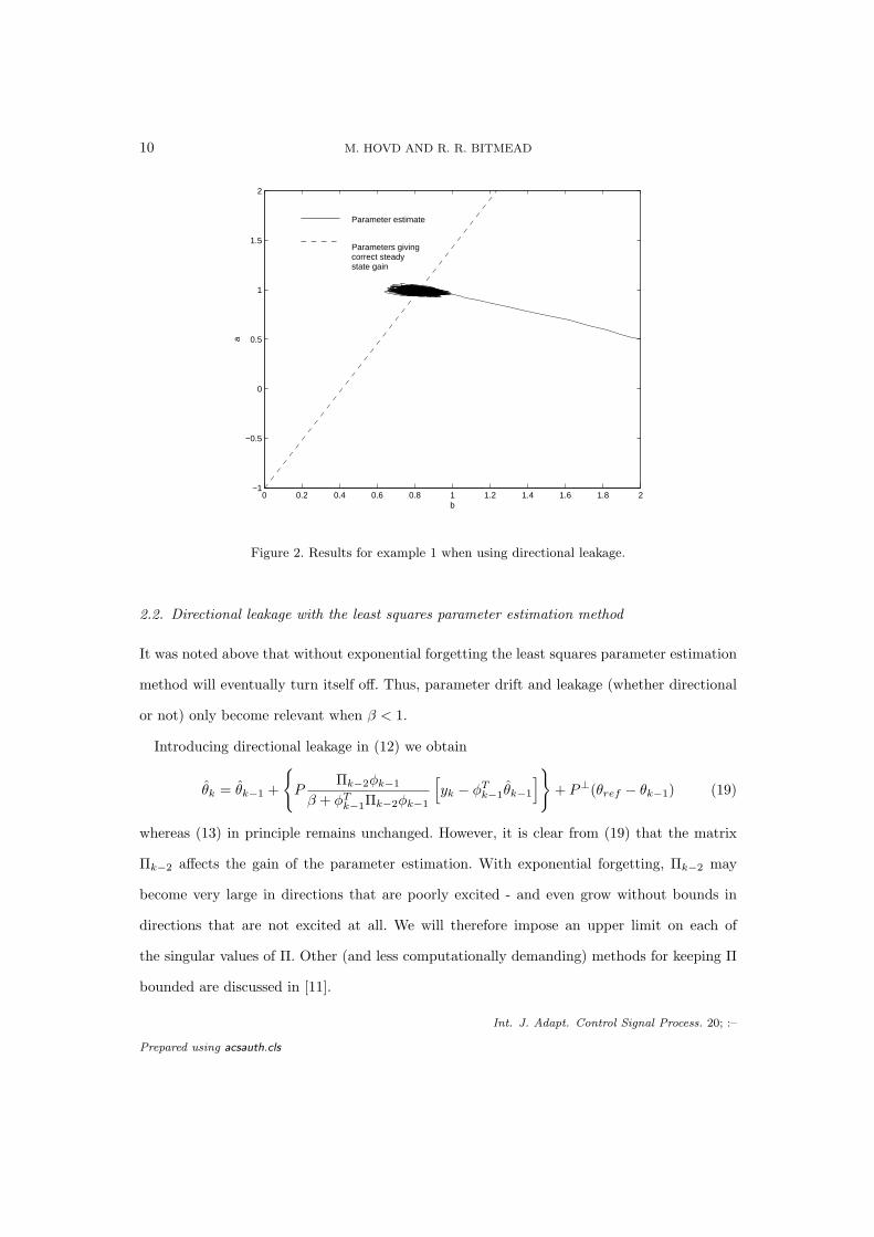
The results obtained when using directional leakage are shown in Fig. 2. The reference values

θref are chosen equal to the initial parameters. The parameter estimates converge to a point

on the line indicating the correct steady state gain, and no significant parameter drift can be

found.




0 0.2 0.4 0.6 0.8 1 1.2 1.4 1.6 1.8 2−1

−0.5

0

0.5

1

1.5

2

a

b

Parameter estimate

Parameters givingcorrect steady state gain

Figure 2. Results for example 1 when using directional leakage.

2.2. Directional leakage with the least squares parameter estimation method

It was noted above that without exponential forgetting the least squares parameter estimation

method will eventually turn itself off. Thus, parameter drift and leakage (whether directional

or not) only become relevant when β < 1.

Introducing directional leakage in (12) we obtain

θk = θk−1 +

{P

Πk−2φk−1


[yk − φT

k−1θk−1

]}+ P⊥(θref − θk−1) (19)

whereas (13) in principle remains unchanged. However, it is clear from (19) that the matrix

Πk−2 affects the gain of the parameter estimation. With exponential forgetting, Πk−2 may

become very large in directions that are poorly excited - and even grow without bounds in

directions that are not excited at all. We will therefore impose an upper limit on each of

the singular values of Π. Other (and less computationally demanding) methods for keeping Π

bounded are discussed in [11].




Proceeding with the analysis for the exponentially weighted least squares, we arrive

at an equation mirroring (17) above. However, we here get that Hi = I −1

β+φTk−1Πk−2φk−1

Πk−2φk−1φTk−1. In evaluating

∏k+s−1i=k PHi, we then face the problem that

in general Πk+m and φk+nφTk+n do not commute. We are therefore unable to arrive at an

equally simple expression as in (18). Instead, we obtain

k+s−1∏

i=k

Hi = P − P (εkΠkXk + εk+1Πk+1Xk+1 + · · ·+ εk+s−1Πk+s−1Xk+s−1)

+ O

((εΠ)2

s(s− 1)2

)(20)

where here εi = 1β+φT

i−1Πi−2φi−1whereas Xi = φi−1φ

Ti−1 as before. The symbols ε and Π

represent average values of εi and Πi, respectively. We find that for sufficiently small Π, the

linear term in (20) will dominate, here ε may well be close to 1. A sufficiently small Π is

obtained by choosing a forgetting factor β close to 1, and effectively constraining growth of

Π in directions that are insufficiently excited. It should be noted that in the directions in the

input-output data that are poorly but persistently excited, Π may grow large unless β is very

close to 1 or the singular values of Π are properly constrained. Still, we can conclude from (20)

that given a sufficiently small Π, the parameter estimation will remain asymptotically stable

provided rank(P ) = rank(P (εkΠkXk +εk+1Πk+1Xk+1 + · · ·+εk+s−1Πk+s−1Xk+s−1) Since Πi

is positive definite for all i, this rank condition is essentially equivalent to the rank condition

found for the gradient method.

Example 2. The use of directional leakage will next be illustrated used on a problem in

adaptive control. The plant is given by

g(z) =2z − 1.8

z3 − 2.78z2 + 2.5715z − 0.79135(21)

The control objective is to track the reference signal

r(t) = sin(2πt

360) + sin(

2πt

45) (22)




Thus, we have five unknown parameters, whereas the reference signal would only be sufficiently

rich to identify four parameters. There is also an additive measurement noise, modelled as a

normally distributed, zero mean random variable with standard deviation 0.04. The control

design is accomplished using adaptive pole placement, using a discrete version of the method

described in [10]. A sampling interval of 1 is used, and all poles of the closed loop characteristic

polynomial are placed at z = 0.7. For the parameter estimation, state variable filters for both

inputs and outputs equal to f(z) = 1(z−0.8)3 are used. The estimation is done with the least

squares method with a forgetting factor β = 0.998. The singular values of Π are constrained to

be no larger than 1e− 4. The initial parameter estimates correspond to the transfer function.

g(z, θ) =2(z − 0.91)

(z − 0.99)(z − 0.93)(z − 0.86)(23)

Although these initial parameter values would appear to be quite good, initial control

performance is appalling. The performance quickly improves, and good performance is obtained

after a short initial transient. Luckily, this paper addresses long term rather than initial

behavior, and parameter estimation rather than control. Similar control performance is

obtained for the simulated time period both without leakage and with directional leakage.

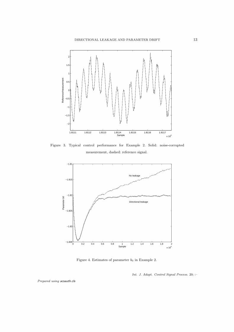
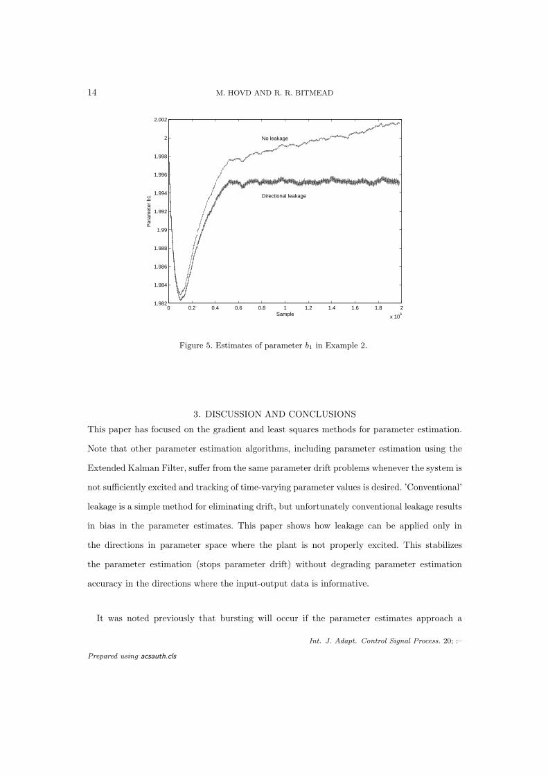
Figure 3 may represent the typical control performance for both cases. The results (Figs. 4

- 8) show that the parameter estimates drift when no leakage is applied. When directional

leakage is applied, the noise does affect the parameter estimates, but no parameter drift can

be seen. The effect of the noise that is seen in the parameter estimates appear have no effect

on the control performance. However, the effect of noise may be reduced by reducing the

maximum singular value bound for the covariance matrix, and/or using a larger forgetting

factor. The forgetting factor of β = 0.998 corresponds to a time constant for forgetting of

500 samples. This may appear to be somewhat too fast when the signal to be tracked has a

sinusoid of period 360.




1.8111 1.8112 1.8113 1.8114 1.8115 1.8116 1.8117

x 106

−2

−1.5

−1

−0.5

0

0.5

1

1.5

2

Sample

Ref

eren

ce/m

easu

rem

ent

Figure 3. Typical control performance for Example 2. Solid: noise-corrupted

measurement, dashed: reference signal.

0 0.2 0.4 0.6 0.8 1 1.2 1.4 1.6 1.8 2

x 106

−1.835

−1.83

−1.825

−1.82

−1.815

−1.81

Sample

Par

amet

er b

0

No leakage

Directional leakage

Figure 4. Estimates of parameter b0 in Example 2.




0 0.2 0.4 0.6 0.8 1 1.2 1.4 1.6 1.8 2

x 106

1.982

1.984

1.986

1.988

1.99

1.992

1.994

1.996

1.998

2

2.002

Par

amet

er b

1

Sample

No leakage

Directional leakage

Figure 5. Estimates of parameter b1 in Example 2.

3. DISCUSSION AND CONCLUSIONS

This paper has focused on the gradient and least squares methods for parameter estimation.

Note that other parameter estimation algorithms, including parameter estimation using the

Extended Kalman Filter, suffer from the same parameter drift problems whenever the system is

not sufficiently excited and tracking of time-varying parameter values is desired. ’Conventional’

leakage is a simple method for eliminating drift, but unfortunately conventional leakage results

in bias in the parameter estimates. This paper shows how leakage can be applied only in

the directions in parameter space where the plant is not properly excited. This stabilizes

the parameter estimation (stops parameter drift) without degrading parameter estimation

accuracy in the directions where the input-output data is informative.

It was noted previously that bursting will occur if the parameter estimates approach a




0 0.2 0.4 0.6 0.8 1 1.2 1.4 1.6 1.8 2

x 106

−0.796

−0.794

−0.792

−0.79

−0.788

−0.786

−0.784

−0.782

Sample

Par

amet

er a

0

No leakage

Directional leakage

Figure 6. Estimates of parameter a0 in Example 2.

hypersurface in parameter space where the model is uncontrollable. Although directional

leakage, when properly tuned, makes the parameter estimation asymptotically stable, that

does not rule out the possibility that during the initial transient the parameters may encounter

such an uncontrollable hypersurface. For problems where this is a serious concern, directional

leakage may easily be combined with so-called parameter projection [10], which constrains the

parameter estimates to stay within an a priori defined region of the parameter space where

the true model is assumed to lie, and which is also assumed to be free of uncontrollable

hypersurfaces.

Thus, despite the advantages of directional leakage noted above, it does not totally eliminate

the problem of bursting. Note, however, that such bursting during initial transients may also

occur when the exciting signals are persistently exciting, if the initial parameter estimates are

ill-chosen. Therefore, any failure to prevent bursting during transient conditions should not be




0 0.2 0.4 0.6 0.8 1 1.2 1.4 1.6 1.8 2

x 106

2.552

2.554

2.556

2.558

2.56

2.562

2.564

2.566

2.568

2.57

2.572

Par

amet

er a

1

Sample

Directional leakage

No leakage


0 0.2 0.4 0.6 0.8 1 1.2 1.4 1.6 1.8 2

x 106

−2.786

−2.784

−2.782

−2.78

−2.778

−2.776

−2.774

−2.772

−2.77

−2.768

Sample

Par

amet

er a

2

No leakage

Directional leakage





considered a shortcoming of (directional) leakage - it is simply not the problem it is intended

to prevent.

The use of a dead-zone (see, e.g., [1]) in the parameter estimation is a common way of

reducing parameter drift. The dead-zone reduces parameter drift by stopping the parameter

update when model predictions are close to the physical measurement. Directional leakage, on

the other hand, does not stop parameter estimation when the model output is close to the

measurement. Since leakage is applied only in the directions in parameter space where the

signals are not informative, the asymptotic model accuracy is not affected. Directional leakage

should therefore be an attractive alternative to the use of dead-zones.

Acknowledgement

The first author got the idea for this paper while attending Miroslav Krstic’s Adaptive Control

class during a sabbatical at UCSD, and wishes to thank prof. Krstic for his inspiring teaching.

REFERENCES

1. B. Egardt. Stability of Adaptive Controllers, volume 20 of Lecture Notes in Control and Information

Sciences. Springer-Verlag, Berlin, Germany, 1979.

2. P. A. Ioannou and P. V. Kokotovic. Instability analysis and improvement of robustness of adaptive control.

Automatica, 20:583–594, 1984.

3. D. A. Lawrence, W. A. Sethares, and W. Ren. Parameter drift instability in disturbance-free adaptive

systems. IEEE Transactions on Automatic Control, 838:584–587, 1993.

4. B. D. O. Anderson. Adaptive systems, lack of persistency of excitation, and bursting phenomena.

Automatica, 21:247–257, 1985.

5. P. A. Ioannou and P. V. Kokotovic. Adaptive Systems with Reduced Models, volume 47 of Lecture Notes

in Control and Information Sciences. Springer-Verlag, Berlin, Germany, 1983.

6. W. A. Sethares, C. R. Johnson, and C. E. Rohrs. Bursting in adaptive hybrids. IEEE Transactions on

Communications, 37:791–799, 1989.

7. W. A. Sethares, D. A. Lawrence, C. R. Johnson, and R. R. Bitmead. Parameter drift in lms adaptive

filters. IEEE Transactions on Acoustics, Speech, and Signal Processing, 34:868–879, 1986.




8. R. R. Bitmead and C. R. Johnson. Discrete Averaging Principles and Robust Adaptive Identification,

volume 25 of Advances in Control and Dynamic Systems, pages 237–271. Academic Press, New York,

1987.

9. G. J. Rey, R. R. Bitmead, and C. R. Johnson. The dynamics of bursting in simple adaptive feedback

systems with leakage. IEEE Transactions on Circuits and Systems, 38:476–488, 1991.

10. P. A. Ioannou and J. Sun. Robust Adaptive Control. Prentice-Hall, Upper Saddle River, New Jersey,

USA, 1996.

11. C. G. Goodwin and K. S. Sin. Adaptive Filtering Prediction and Control. Prentice-Hall, Englewood

Cliffs, New Jersey, USA, 1984.

Int. J. Adapt. Control Signal Process. 20; :–Prepared using acsauth.cls

Directional leakage and parameter driftoodgeroo.ucsd.edu/~bob/docs/P79_Morten_IJACSP_draft.pdf ·...

Documents

Transcript of Directional leakage and parameter driftoodgeroo.ucsd.edu/~bob/docs/P79_Morten_IJACSP_draft.pdf ·...