Directional analysis of 3D tubular structures via

isotropic well-localized atoms

David Jimeneza, Demetrio Labateb, Manos Papadakis

aDepartment of Mathematics, University of Costa Rica, Costa RicabDepartment of Mathematics, University of Houston, Houston, TX, 772014-3308, USA

Abstract

Accurate segmentation of 3D vessel-like structures is a major challenge inmedical imaging. In this paper, we introduce a novel approach for the de-tection of 3D tubular structures that is particularly suited to capture the ge-ometry of vessel-like networks, such as dendritic trees and vascular systems.Even though our approach relies on a system of isotropic multiscale analyzingatoms, we prove that their interaction via convolution with a tubular struc-ture is equivalent to a set of directional atoms at various scales, automaticallyoriented along any possible direction and with cylindrical symmetry. Thisresult sets the theoretical groundwork for the design of efficient discrete al-gorithms aiming at extracting the geometry of vessel-like structures in 3Dmedical images.

Keywords: Directional representations, isotropic filters, tubular structures,Laplacian filters, steerable filters2012 MSC: 42C40

1. Introduction

This paper presents a new method for the detection and geometric char-acterization of tubular structures in 3D images. This study is motivated bythe problem of segmenting and reconstructing the morphological propertiesof vessel-like structures in medical images, such as vascular networks in thelungs or the liver, dendritic arbors and axons in brain tissues and neuronalcultures.

Email addresses: david.jimenezlopez@ucr.ac.cr (David Jimenez ),dlabate@math.uh.edu (Demetrio Labate), mpapadak@math.uh.edu (Manos Papadakis)

Preprint submitted to Elsevier November 18, 2014

Processing these types of images presents several challenges, due to thecomplex 3D topology and the significant variations in size, orientation andintensity contrast of the vessel-like structures that need to be detected inimages. Due to large variations in size of objects of interest, a number ofideas based on multiscale analysis have been proposed for the analysis andthe preprocessing of such data. Koller at al. [16], in particular, introduceda multiscale filter based on the eigenvectors of the Hessian matrix of theimage, to detect highly elongated objects. Following this work, other suc-cessful studies have focused on the eigenvalues of the Hessian matrix to detecttubular structures (cf. [17] and references therein).

During the last decade, the emergence of more sophisticated multiscalemethods has further expanded the range of tools available for the analysisof geometric features of multidimensional data. Among these methods thereare several ‘directional’ representations where the analyzing functions aredefined not only across several scales but also at several orientations, suchas beamlets [6], ridgelets [3], curvelets [4] and shearlets [8, 21]. Thanks to acombination of multiscale analysis and directional sensitivity, these methodscan provide highly sparse representations of images with edges [4, 8, 19].Indeed, directional multiscale transforms derived from these representationscan be especially effective at capturing the geometry of multidimensionalsingularities through their asymptotic decay at fine scales [5, 18]. Theseproperties can be very useful in the analysis of biomedical images containinghighly elongated structures as illustrated by recent applications to fluorescentimages of brain tissue and neuronal cultures [20, 23, 24].

Remarkably, in this paper we show that it is to possible capture the geo-metric characteristics of a 3D tubular structure, regardless of its spatial ori-entation, using rather conventional multiscale 3D isotropic Laplacian filters.As we prove in this paper, when applied to tubular structures these filtersact as two-dimensional Laplacians at the direction of the gradient of the in-tensity level of the image. In other words, the interaction via convolution ofa set of isotropic multiscale atoms with a tubular structure is equivalent tothe action of a set of directional multiscale 3D atoms, aligning themselves tothe tubular structure and with cylindrical symmetry. Hence, the convolutionof these atoms produce rotationally covariant outputs obeying very simplecovariance rules (cf. Theorem 1 in Sec. 2), although the analyzing atomsof the underlying representation are not intrinsically steerable, in the sensethat there is no external mechanism to steer them. They act as self-steerableatoms when they interact with tubular structures.

2

This finding is quite reminiscent of Marr’s claim that low-level vision isbased on the detection of intensity changes of luminosity modeled by fil-tering an image with an isotropic Laplacian operator windowed by a two-dimensional isotropic Gaussian [22, p. 54]. Such models are supported byneurophysiological findings according to which the retinal photoreceptors arespatially organized ([7], Ch. 1, also see [22], pp. 64–65, and [25]) so that:

(a) “They provide high or low spatial and temporal resolution images ofevery scene depending on the prevailing conditions of observation; thetemporal resolution equips the eyes with the perception of motion andthe capability of detecting sudden stimulus onsets, while the spatialresolution primarily contributes to object recognition ([7], Ch. 1);

(b) edges (boundaries where the luminosity abruptly changes) are observedregardless of their orientation or topology.”

By no means we claim that our collection of isotropic atoms yields a direc-tional representation in the sense of a ‘true’ directional multiscale systems,where the analyzing atoms range over a set of prescribed orientations. Infact, the directional sensitivity of our isotropic atoms only arises in the pres-ence of tubular structures and we consider these atoms as analyzing elementsonly (they cannot be used for synthesis). Another difference is that ‘true’directional multiscale transforms are able to detect location and orientationof edge singularities through their asymptotic decay at fine scales, while ourapproach does not detect edges (see also the related discussion in the lastsection) neither can it identify the local orientation of the tubular structure,but it is effective at capturing the geometry of tubular structures at a specificrange of scales.

With respect to directional multiscale representations, isotropic multi-scale filters have lower redundancy, leading to discrete implementations withlower computational cost. This can be a significant advantage especially forthe processing of 3D data.

2. Directional filtering of tubular structures using isotropic atoms

We begin by introducing a generic class of tubular structures in R3 thatcan be used to model dendritic branches of neurons, blood vessels and similarbiological structures.

3

2.1. Modeling tubular structures

To define such tubular structures, we start by considering the tubularsegments defined as tensor products of the form:

fl,L,r(x, y, z) = gl,L(x)gr(y, z), x, y, z,∈ R, r > 0, (1)

where gl,L is even, non-increasing on the positive half axis and satisfies

gl,L(x) = 1 if 0 ≤ x ≤ lgl,L(x) > 0 if l < x < Lgl,L(x) = 0 if L ≤ x;

the second factor satisfies gr(y, z) ≥ 0 and gr(y, z) = 0 when y2 + z2 ≥ r2.In (1), the term gl,L controls the length of the structure, which extends

along the x-axis, while the second factor controls the decay of the imageintensity values in a cross-section. In the following, we will assume thatthe first and second-order derivatives of gl,L and of gr are both absolutelyintegrable, so gl,L and g′l,L and g′r are both absolutely continuous. In orderto allow more flexibility in the shape of “tubular” cross sections, we make nospecial symmetry assumptions on the term gr.

Clearly, the tubular segments given by (1) can be translated via the actionof translation operators Txk , xk ∈ R3, defined by Txkf(x) = f(x − xk)and re-oriented by means of rotations Rk ∈ SO(3). For any such a 3Drotation matrix Rk, we define the rotation operator Rk by Rkf(x, y, z) =f(Rk(x, y, z)). Therefore, we define a tubular structure I as finite sum of theform

I =K∑k=1

ak TxkRkflk,Lk,rk , (2)

where the terms flk,Lk,rk are tubular segments and the quantities ak arestrictly positive constants controlling the image intensity in each tubularsegment.

This model of tubular structures is adequate, in particular, to modeldendritic branches in neurons where the centerline can be approximated bya polygonal curve. In our model, the intensity value along the centerline ofany component TxkRkflk,Lk,rk is constant. Even though in typical fluorescentimages of neurons the fluorescent signal intensity is not constant, it is rea-sonable to assume that the intensity value does not vary too rapidly so thatwe can assume it to be constant along the centerline of a tubular segment, ifthis is sufficiently short.

4

2.2. Analysis of tubular segments

We start by examining the action of a simple family of isotropic trans-formations on the tubular segments TxkRkflk,Lk,rk , for generic xk ∈ R3,Rk ∈ SO(3).

Let φ ∈ L2(R3) be a radial function such that all its derivatives up secondorder are absolutely integrable and such that ξ 7→ ||ξ||2φ(ξ) is also absolutelyintegrable and bounded. Let h be defined by

h(ξ) := ||ξ||2φ(ξ), ξ ∈ R3. (3)

Using a change of variables and the radiality of h, we observe that

(TxkRkflk,Lk,rk ∗ h)(x) =

∫R3

flk,Lk,rk (Rk(x− xk)− s)h(RTk s)ds

= flk,Lk,rk ∗ h (Rk(x− xk)) . (4)

Clearly, the same equality is also valid with φ instead of h:

(TxiRkflk,Lk,rk ∗ φ)(x) = flk,Lk,rk ∗ φ (Rk(x− xk)) . (5)

The continuity of flk,Lk,rk and the integrability of h imply that

flk,Lk,rk ∗ h (Rk(x− xk)) =

∫R3

flk,Lk,rk(ξ) φ(ξ) ||ξ||2e2πiξ·(Rk(x−xk))dξ

= ∆(flk,Lk,rk ∗ φ) (Rk(x− xk)) .

Therefore, we conclude that

(TxkRkflk,Lk,rk ∗ h)(x)

= ∆(flk,Lk,rk ∗ φ) (Rk(x− xk))

=∂2

∂x2(flk,Lk,rk ∗ φ)(x0) +

(∂2

∂y2+

∂2

∂z2

)(flk,Lk,rk ∗ φ)(x0), (6)

where x0 = Rk(x − xk). Equation (6) shows that the 3D Laplacian ofthe filtered output of the tubular segment has two components: the axialand the cross-sectional 2D Laplacian. In Theorem 1 we prove that, if xis sufficiently far from the endpoints of the tubular segment, the first termin (6) is negligible whereas the second term is practically equal to the 3DLaplacian. This shows that the action of the isotropic filters on the tubular

5

structure is essentially equivalent to the action of cylindrically symmetricdirectional filters. We also remark that, in the derivation of (6), we did notassume any symmetry in the cross-sections of the tubular structure fl,L,r. Weuse the term ‘tubular’ for such structures without necessarily implying anytype of symmetry (e.g., radial symmetry) in the cross section.

Before stating our main theorem, we need some preparation.We pick an accuracy threshold ε > 0 and we assume that x0 is sufficiently

away from both ends of the support of the tubular segment flk,Lk,rk . Thisimplies that the support of φ is relatively smaller than the support of thetubular segment, so that |x0 · e1|+r0 < l. Therefore, with no loss of generalitywe can shift the axial center of the tubular segment from the origin to anotherpoint on the x-axis so that x0 = (0, y0,1, z0,1). Now, the integrability of

ξ 7→ ||ξ||2φ(ξ) and the Riemann-Lebesgue lemma imply that there existsr0 > 0 such that |Dαφ(y)| < min{ε/2L, ε}, if ||y|| ≥ r0 and |α| ≤ 2.

On the other hand, the integrability of the partial derivatives of φ up tosecond order allows us to select r0 so that

∫|x|>r0 |D

αφ| < ε for all |α| ≤ 2.

These two observations are summarized in the following lemma.

Lemma 1. Let ε > 0 and φ ∈ L1(R3) be a radial function such that ξ 7→||ξ||2φ(ξ) is absolutely integrable and Dαφ ∈ L1(R3) for all |α| ≤ 2. Thenthere exists r0 > 0 such that:

1. |Dαφ(y)| < min{ε/2L, ε} if ||y|| ≥ r0 and |α| ≤ 2;

2.∫|x|>r0 |D

αφ| < ε.

In other words, we can choose a filter φ with sufficient smoothness andspatial localization. In practical situations, like the numerical exampleswhich will be considered further below, we don’t use a single filter φ buta set of filters ranging over different scales, from fine to coarse, provided thatwe maintain the requirement |x0 · e1| + r0 < l. Filters with bigger r0 aresuitable for thicker and longer tubular segments while filters with smaller r0are fit for short and thin tubular segments. This heuristic statement will beformalized in Proposition 1.

We are now ready to state the main result of this work establishing thatthe isotropic filters φ and h act as directional filters when they are appliedto a tubular segment.

In the following, we use the convention e1 = (1, 0, 0), e2 = (0, 1, 0) ande3 = (0, 0, 1) and we denote by x(x0), y(x0) and z(x0) the various coordinatesof the vector x0 = R(x− xk).

6

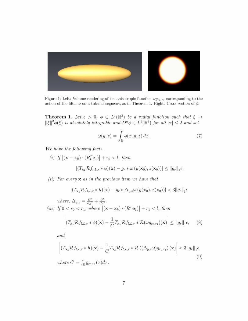
Figure 1: Left: Volume rendering of the anisotropic function ωgr0,r1 corresponding to theaction of the filter φ on a tubular segment, as in Theorem 1. Right: Cross-section of φ.

Theorem 1. Let ε > 0, φ ∈ L1(R3) be a radial function such that ξ 7→||ξ||2φ(ξ) is absolutely integrable and Dαφ ∈ L1(R3) for all |α| ≤ 2 and set

ω(y, z) =

∫Rφ(x, y, z) dx. (7)

We have the following facts.

(i) If∣∣(x− xk) · (RT

k e1)∣∣+ r0 < l, then

|(TxkRfl,L,r ∗ φ)(x)− gr ∗ ω (y(x0), z(x0))| ≤ ||gr||1ε.

(ii) For every x as in the previous item we have that

|(TxkRfl,L,r ∗ h)(x)− gr ∗∆y,zω (y(x0), z(x0))| < 3||gr||1ε

where, ∆y,z = ∂2

∂y2+ ∂2

∂z2.

(iii) If 0 < r0 < r1, where∣∣(x− xk) · (RTe1)

∣∣+ r1 < l, then∣∣∣∣(TxkRfl,L,r ∗ φ)(x)− 1

CTxkRfl,L,r ∗ R(ωgr0,r1)(x)

∣∣∣∣ ≤ ||gr||1ε, (8)

and∣∣∣∣(TxkRfl,L,r ∗ h)(x)− 1

CTxkRfl,L,r ∗ R ((∆y,zω)gr0,r1) (x)

∣∣∣∣ < 3||gr||1ε,

(9)where C =

∫R gr0,r1(x)dx.

7

Before presenting the proof of Theorem 1, we will make some remarks tohighlight the significance of the theorem.

Part (ii) of the theorem states that filtering the tubular segment usingthe 3D Isotropic Laplacian filter h is equivalent to applying the 2D Laplacianon the cross-section of the tubular structure TxiRfl,L,r. Part (iii) statesthat filtering using the 3D isotropic filters φ and h is equivalent to applyingdirectional filters that automatically align themselves with the axis of thetubular structure (see Fig. 2.2). The orientation of the tubular segment isdetermined by the rotation Rk which orients its main axis along the directionRTk e1. According to (iii), the main axis of the directional filters Rk(ωgr0,r1)

and Rk ((∆y,zω)gr0,r1) is also parallel to RTk e1. This is why we claim that

filtering with the radial filters φ and h is equivalent to filtering with thedirectional filters 1

CRk(ωgr0,r1) and 1

CRk ((∆y,zω)gr0,r1), respectively, which

are automatically aligned with the tubular structure locally at the pointx. The former of the two filters acts as a directional lowpass, bandpassor highpass filter depending on the frequency selectivity of φ. The latterfilter acts as a 2D Laplacian on a plane perpendicular to the direction of thetubular structure as (ii) shows.

Note that the outcome of the filtering process of the tubular segmentusing φ and h depends only on the relative position of the point x with re-spect to the cross-section of the tubular containing x and on the propertiesof this cross-section. The similarity of the action of the filters φ and h totruly directional filters is due solely to the geometry of the tubular segment,as one can verify by the proof of Theorem 1 below. Thus, our result es-tablishes that a seemingly directionally insensitive system of atoms acts asa directional filter in certain conditions and is able to detect the geometriccontent associated with highly anisotropic objects. This ability to detectthe geometry of elongated features is somewhat reminiscent of the propertiesof directional multiscale transform such the continuous shearlet transform,which was recently applied to detect the geometry of singularities of functionsand distributions of several variables [9, 10]. However, there is an importantdifference here: the shearlet result for the detection of singularities is validonly asymptotically, when the scale variable tends to zero, whereas the re-sult we derive here is valid over a range of scale associated with the spatialdimensions of the objects of interest.

In Section 3, we will briefly discuss the implications of these theoreticalobservations for the segmentation of tubular structures in biomedical images.

8

2.3. Proof of Theorem 1

We can now prove Theorem 1.(i) Without loss of generality, we can take x0 = (0, y0,1, z0,1). A direct

calculation gives that

fl,L,r ∗ φ(x0) =

∫R

∫Rgr(y, z)

(∫Rgl,L(x)φ(−x, y0,1 − y, z0,1 − z)dx

)dydz.

Using (7) it follows that

fl,L,r ∗ φ(x0)− gr ∗ ω(y0,1, z0,1)

=

∫R2

gr(y, z)(

∫Rgl,L(x)φ(−x, y0,1 − y, z0,1 − z)dx− ω(y0,1 − y, z0,1 − z))dydz.

We can split the above integral by integrating over two complementary radialregions:∫

Rgl,L(x)φ(−x, y0,1 − y, z0,1 − z)dx =

∫|x|≤r0

(. . . ) +

∫|x|>r0

(. . . ).

Consequently, using the fact that gl,L(x) = 1 for all |x| ≤ r0, we have

fl,L,r ∗ φ(x0)− gr ∗ ω(y0,1, z0,1)

=

∫R

∫Rgr(y, z)

[∫|x|>r0

[gl,L(x)− 1]φ(−x, y0,1 − y, z0,1 − z)dx

]dydz.

Observing that 0 ≤ gl,L(x) ≤ 1 for all x and∫|x|>r0 |φ| < ε (Lemma 1), we

conclude that

|fl,L,r ∗ φ(x0)− gr ∗ ω(y0,1, z0,1)| ≤ ||gr||1ε.

This inequality combined with (5) proves part (i).(ii) We begin by showing that the first term of the sum in the right-hand

side of (6) is less than 2ε:

∂2

∂x2(gl,Lgr ∗ φ)(x0)

=

(gr

∂2gl,L∂x2

)∗ φ(x0)

=

∫R

∫Rgr(y, z)

(∫R

∂2gl,L∂x2

(x)φ(−x, y0,1 − y, z0,1 − z)dx

)dydz (10)

9

and again we write∫R

∂2gl,L∂x2

(x)φ(−x, y0,1 − y, z0,1 − z)dx =

∫|x|≤r0

(. . . ) +

∫|x|>r0

(. . . ).

The first of the two terms in the integral above vanishes because gl,L(x) = 1for all |x| < l. To estimate the second term we apply twice integration byparts using gl,L(±L) = g′l,L(±r0) = g′l,L(±L) = 0 and gl,L(±r0) = 1:∫

|x|>r0

∂2gl,L∂x2

(x)φ(−x, y0,1 − y, z0,1 − z)dx

=

∫|x|>r0

∂2φ

∂x2(−x, y0,1 − y, z0,1 − z)gl,L(x)dx+

∂φ

∂x(r0, y0,1 − y, z0,1 − z).

Thus we have that:∣∣∣∣∫|x|>r0

∂2gl,L∂x2

(x)φ(−x, y0,1 − y, z0,1 − z)dx

∣∣∣∣ < 2ε.

Using eqs. (6) and (10) we conclude that:

|(TxkRkfl,L,r ∗ h)(x)−∆y,z(fl,L,r ∗ φ)(x0)| < 2||gr||1ε . (11)

Since Dαφ ∈ L1(R3) for all |α| ≤ 2, we have that

∆y,z(fl,L,r ∗ φ)(x0) = fl,L,r ∗ (∆y,zφ)(x0) (12)

and, hence,∫R

∆y,zφ(−x, y0,1 − y, z0,1 − z)dx = ∆y,zω(y0,1 − y, z0,1 − z),

for all y, z ∈ R. It follows that∫R

∆y,zφ(−x, y0,1 − y, z0,1 − z)gl,L(x)dx−∆y,zω(y0,1 − y, z0,1 − z)

=

∫|x|>r0

[gl,L(x)− 1]∆y,zφ(−x, y0,1 − y, z0,1 − z) dx.

Now, arguing as in the proof of part (i) and using eq. (12), we obtain that

|fl,L,r ∗ (∆y,zφ)(x0)− gr ∗ (∆y,zω)(y0,1, z0,1)| ≤ ||gr||1ε .

10

Combining the previous inequality with (11), we complete the proof of part (ii).(iii) Using again the change of variables leading to eq. (4) we have that

TxkRkfl,L,r ∗ Rk(ωgr0,r1)(x) = fl,L,r ∗ (ωgr0,r1)(x0).

Now, let x(x0) be the x-coordinate of x0. Then:

fl,L,r ∗ (ωgr0,r1)(x0) = gr ∗ ω(y0,1, z0,1)

∫Rgl,L (x(x0)− x) gr0,r1(x)dx(13)

= Cgr ∗ ω(y0,1, z0,1),

since gl,L (x(x0)− x) = 1 for all |x| < r1, due to the observations that∣∣(x− xk) · (RTk e1)

∣∣ + r1 < l. Combining eq. (13) and part (i) we deriveeq. (8). Eq. (9) can be derived with similar arguments. This completes theproof of Theorem 1. �

2.4. Other results

The following observation is useful to determine the filter h so that itcan accurately capture the change in the sign of ∆y,zgr. Here we provide aformal statement on the dependence of the choice of r0 on r. Recall, thatthe latter is a metric indicative of the thickness of the tubular structure.Failure to choose the filter φ with the appropriate bandwidth r0 will resultin aliasing errors that will compromise the detection of the surface of thetubular structure.

Proposition 1. Assume that the hypotheses of Theorem 1 hold true and

suppose that∣∣∣1− φ(ξ)

∣∣∣ < ε for a.e. ||ξ|| < ρ, where ρ is determined by∫||(ξ2,ξ3)||>ρ

gr(ξ2, ξ3)(ξ22 + ξ23)dξ2dξ3 <

ε

1 + ||φ||1. (14)

Then, for every xi and rotation Rk, we have that

|(TxiRkfl,L,r ∗ h)(x)−∆y,zgr (y(x0), z(x0))| ≤ (3||gr||1 + 1)ε

for every x that is sufficiently far from the endpoints of the tubular structureTxiRkfl,L,r, in the sense that

∣∣(x− xi) · (RTk e1)

∣∣+ r0 < l.

11

Proof: A direct computation shows that

|(TxiRkfl,L,r ∗ h)(x)−∆y,zgr (y(x0), z(x0))|

= |(TxiRkfl,L,r ∗ h)(x)− gr ∗∆y,zω (y(x0), z(x0))

−∆y,zgr (y(x0), z(x0)) + gr ∗∆y,zω (y(x0), z(x0)) |

≤ |(TxiRkfl,L,r ∗ h)(x)− gr ∗∆y,zω (y(x0), z(x0))|

+|gr ∗∆y,zω (y(x0), z(x0))−∆y,zgr (y(x0), z(x0))|.

By part (ii) of Theorem1 we know that the first term of the sum above doesnot exceed 3||gr||1ε. Next, we will show that the second term in the sum isbounded above by 3ε. By computing the Fourier transform of second term,we get

(gr ∗∆y,zω−∆y,zgr)∧(ξ2, ξ3) = gr(ξ2, ξ3)(ξ

22 + ξ23)ω(ξ2, ξ3)− gr(ξ2, ξ3)(ξ22 + ξ23).

(15)We have that:∫

R2

∣∣gr(ξ2, ξ3)(ξ22 + ξ23)ω(ξ2, ξ3)− gr(ξ2, ξ3)(ξ22 + ξ23)∣∣ dξ2 dξ3

=

∫R2

gr(ξ2, ξ3)(ξ22 + ξ23)|ω(ξ2, ξ3)− 1| dξ2 dξ3

≤∫||(ξ2,ξ3)||≤ρ

gr(ξ2, ξ3)(ξ22 + ξ23)|ω(ξ2, ξ3)− 1| dξ2 dξ3

+

∫||(ξ2,ξ3)||≥ρ

gr(ξ2, ξ3)(ξ22 + ξ23)(|ω(ξ2, ξ3)|+ 1) dξ2 dξ3.

Now, using the assumption that∣∣∣1− φ(ξ)

∣∣∣ < ε for a.e. ||ξ|| < ρ, (14), (15)

and the fact ω(ξ2, ξ3) = φ(0, ξ2, ξ3) for a.e. (ξ2, ξ3), we conclude that

|(TxiRkfl,L,r ∗ h)(x)−∆y,zgr (y(x0), z(x0))| ≤ (3||gr||1 + 1)ε (16)

This completes the proof of Proposition 1. �

An example of a filter φ satisfying the assumptions of Proposition 1 isgiven by

φ(ξ) = Pn(Cn,σ‖ξ‖2

)e−Cn,σ‖ξ‖

2

,

12

where Pn is the Taylor polynomial of degree n associated with the exponentialfunction ex, the constant Cn,σ is

Cn,σ =2n+ 1

2(Kσ)2,

and σ is a parameter associated with a notion of scale. This filter belongs tothe class of Hermite Distributed Approximating Functions that were origi-nally proposed by Hoffman et. al. in [13]. The choice of the constant Cn,σplaces the inflection point of the radial profile of φ firmly at radius Kσ fromthe origin, regardless of the value of n. As n increases to ∞ (cf. [1, Remark3.4]), the width of the radial profile of the transition band of φ is propor-tional to 1

n. This transition band also contains the inflection point of the

radial profile of φ, for every n. Moreover, as n grows, the values of φ tendto 1 at every point in the ball centered at the origin with radius Kσ ([1, Th.3.7]). In a nutshell, φ asymptotically behaves like an isotropic ideal low passfilter.

So far our analysis was focused on a single segment TxiRkfl,L,r of thetubular structure I given by (2). The proposed filters φ and h can be appliedto the entire tubular structure I. Recall that, in Theorem 1, we assumedthat the point x is close only to a single tubular segment of I. Due tothe spatial localization of the filters φ and h, each tubular segment can beprocessed independently of the others. This observation leads to the followingcorollary.

Corollary 1. Under the assumptions of Theorem 1, we have that

|(I ∗ φ)(x)− gr ∗ ω (y(x0), z(x0))| = O(ε) ,

and|(I ∗ h)(x)− gr ∗∆y,zω (y(x0), z(x0))| = O(ε) ,

where x0 = Rk(x − xi) and where the index i, the cross-section gr and therotation Rk correspond to the most proximal segment TxiRkfl,L,r of I to x.Consequently, we have that

|(I ∗ h)(x)−∆y,zgr (y(x0), z(x0))| = O(ε).

13

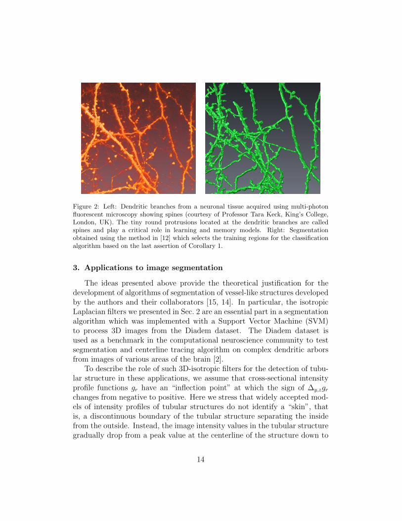
Figure 2: Left: Dendritic branches from a neuronal tissue acquired using multi-photonfluorescent microscopy showing spines (courtesy of Professor Tara Keck, King’s College,London, UK). The tiny round protrusions located at the dendritic branches are calledspines and play a critical role in learning and memory models. Right: Segmentationobtained using the method in [12] which selects the training regions for the classificationalgorithm based on the last assertion of Corollary 1.

3. Applications to image segmentation

The ideas presented above provide the theoretical justification for thedevelopment of algorithms of segmentation of vessel-like structures developedby the authors and their collaborators [15, 14]. In particular, the isotropicLaplacian filters we presented in Sec. 2 are an essential part in a segmentationalgorithm which was implemented with a Support Vector Machine (SVM)to process 3D images from the Diadem dataset. The Diadem dataset isused as a benchmark in the computational neuroscience community to testsegmentation and centerline tracing algorithm on complex dendritic arborsfrom images of various areas of the brain [2].

To describe the role of such 3D-isotropic filters for the detection of tubu-lar structure in these applications, we assume that cross-sectional intensityprofile functions gr have an “inflection point” at which the sign of ∆y,zgrchanges from negative to positive. Here we stress that widely accepted mod-els of intensity profiles of tubular structures do not identify a “skin”, thatis, a discontinuous boundary of the tubular structure separating the insidefrom the outside. Instead, the image intensity values in the tubular structuregradually drop from a peak value at the centerline of the structure down to

14

the range of background values. This principle is reflected in the adoptedmodel of cross-sectional intensity values in and out of the tubular structure,formally presented by gr in Sec. 2. Hence, we postulate that the ‘boundary’ ofthe tubular structure is located at some intermediate radial distance from thecenterline of the structure, preferably at the radial distance of this “inflectionsurface” from the centerline. Then, based on the theoretical predictions ofCorollary 1, we expect I ∗ h to have positive sign right outside the bound-ary of the tubular structure, because I ∗ h is practically equal to ∆y,zgr, the2D-Laplacian on the cross-section of I containing x. Further away from thisboundary, the error of the approximation of the values of ∆y,zgr predictedby Proposition 1 and the response of the application of h to its other prox-imal segments force the sign of I ∗ h to vary. According to these remarks,the problem of segmenting a tubular structure from the background is notposed as an edge detection problem in 3D. Rather, the successful extractionof the geometric features of the tubular structures can be achieved using aset of Laplacian isotropic filters with varying bandwidths, as Proposition 1suggests.

The justification of the adopted model of tubular structure is verifiedindirectly by the high accuracy of our segmentations and centerline trac-ing reported in [15, 14, 11, 12] where the performance of this approach iscompared with state-of-the-art methods from the literature. For example,the application of our centerline tracing algorithm in [14] to volumes fromthe Diadem set yields Miss-Extra-Score (MES) = 0.93 as compared with thestate-of-the-art algorithm of Xie et al. [26] that yields MES = 0.86 (MESis a standard performance metric, where higher values indicate better per-formance, cf. [14]). One of the advantages of our theoretical formalizationis to enable the automatization of the selection process for the training sub-sets of the SVM-classifier used in the segmentation algorithm. We illustratean example of application of this algorithm in Fig. 2, showing the segmen-tation of a complex dendritic network from a brain tissue acquired usingtwo-photon fluorescent microscopy. These images are acquired in vivo andare very challenging to segment due to the high level of noise produced dur-ing data acquisition. Note that the flexibility permitted by our modellingof tubular structures in Sec. 2 enables us to derive an algorithmic approachwhich is effective not only for the detection of the main dendritic branches,but also for the detection of their fine-scale details. As the figure shows,the segmentation algorithm is able to capture also the dendritic spines, tinyprotrusions emerging from dendritic branches which play a very significant

15

role in many cognitive and pharmacological models of the brain.Acknowledgment: This work was supported in part by NSF-DMS

1320910, 0915242, 1008900, 1005799 and by NHARP-003652-0136-2009. Wethank Prof. T. Keck of King’s College, London, UK, for providing the dataof Fig. 2 and P. Hernandez-Herrera for sharing his segmentation algorithmfrom [12]. We also thank Prof. I.A. Kakadiaris of the University of Houstonand Prof. F. Laezza of the University of Texas Medical Branch in Galvestonfor helpful discussions on neuroscience imaging.

References

[1] Bodmann, B., Hoffman, D., Kouri, D., Papadakis, M., 2007. Hermitedistributed approximating functionals as almost-ideal low-pass filters.Sampling Theory in Image and Signal Processing 7, 15–38.

[2] Brown, K., Barrionuevo, G., Canty, A., Paola, V., Hirsch, J., Jefferis,G., Lu, J., Snippe, M., Sugihara, I., Ascoli, G., 2011. The DIADEM datasets: representative light microscopy images of neuronal morphology toadvance automation of digital reconstructions. Neuroinformatics 9 (2-3),143–157.

[3] Candes, E., Donoho, David L., 1999. Ridgelets: a key to higher-dimensional intermittency? Philosophical Transactions of the Royal So-ciety A: Mathematical, Physical and Engineering Sciences 357 (1760),2495–2509.

[4] Candes, E. J., Donoho, D. L., 2004. New tight frames of curvelets and op-timal representations of objects with piecewise C2 singularities. Comm.Pure Appl. Math. 57 (2), 219–266.

[5] Candes, E. J., Donoho, D. L., 2005. Continuous curvelet transform: I.resolution of the wavefront set. Appl. Comp. Harm. Analysis 19, 162–197.

[6] Donoho, D., Huo, X., 2002. Beamlets and multiscale image analysis. In:Barth, T. J., Chan, T., Haimes, R. (Eds.), Multiscale and Multiresolu-tion Methods. Vol. 20 of Lecture Notes in Computational Science andEngineering. Springer Berlin Heidelberg, pp. 149–196.

16

[7] Farah, M., 2000. The cognitive neuroscience of vision. Blackwell Pub-lishers, Malden, MA.

[8] Guo, K., Labate, D., 2007. Optimally sparse multidimensional represen-tation using shearlets. SIAM J. Math. Analysis 39 (1), 298–318.

[9] Guo, K., Labate, D., 2009. Characterization and analysis of edges usingthe continuous shearlet transform. SIAM J. Imaging Sciences 2 (3), 959–986.

[10] Guo, K., Labate, D., 2012. Characterization of piecewise smooth sur-faces using the 3D continuous shearlet transform. J. Fourier Anal. Appl.18, 488–516.

[11] Hernandez-Herrera, P., Papadakis, M., Kakadiaris, I., 2014. Multi-scalesegmentation of neurons based on one-class classification, under review.

[12] Hernandez-Herrera, P., Papadakis, M., Kakadiaris, I., Apr 28 - May2 2014. Segmentation of neurons based on one-class classification. In:Proc. IEEE International Symposium in Biomedical Imaging. Beijing,China.

[13] Hoffman, D. K., Nayar, N., Sharafeddin, O. A., Kouri, D. J., 1991.Analytic banded approximation for the discretized free propagator. J.Phys. Chem. 95, 8299–8305.

[14] Jimenez, D., Labate, D., Kakadiaris, I., Papadakis, M., 2014. Improvedautomatic centerline tracing for dendritic and axonal structures, Neu-roinformatics. in press.

[15] Jimenez, D., Papadakis, M., Labate, D., Kakadiaris, I., April 8-11 2013.Improved automatic centerline tracing for dendritic structures. In: Proc.International Symposium on Biomedical Imaging: From Nano to Macro.San Francisco, CA, pp. 1050–1053.

[16] Koller, T., Gerig, G., Szekely, G., Dettwiler, D., Jun 1995. Multiscale de-tection of curvilinear structures in 2-d and 3-d image data. In: ComputerVision, 1995. Proceedings., Fifth International Conference on ComputerVision. pp. 864–869.

17

[17] Krissian, K., Malandain, G., Ayache, N., Vaillant, R., Trousset, Y.,2000. Model based detection of tubular structures in 3d images. Com-puter Vision and Image Understanding 80 (2), 130–171.

[18] Kutyniok, G., Labate, D., 2009. Resolution of the wavefront set usingcontinuous shearlets. Trans. Amer. Math. Soc. 361, 2719–2754.

[19] Kutyniok, G., Lim, W.-Q., 2011. Compactly supported shearlets areoptimally sparse. Journal of Approximation Theory 163 (11), 1564–1589.

[20] Labate, D., Laezza, F., Ozcan, B., Negi, P., Papadakis, M., 2014. Effi-cient processing of fluorescence images using directional multiscale rep-resentations. Math. Model. Nat. Phenom. 9 (5), 177–193.

[21] Labate, D., Lim, W., Kutyniok, G., Weiss, G., January 2005. Sparsemultidimensional representation using shearlets. In: Unser, M. (Ed.),Proc. Wavelets XI. Vol. 5914 of SPIE Proceedings. pp. 247–255.

[22] Marr, D., 1982. Vision, A computational investigation into the humanrepresentation and processing of visual information. W.H. Freeman andCo., New York, NY.

[23] Ozcan, B., Jimenez, D., Hernandez-Herrera, P., Labate, D., Kakadi-aris, I., Papadakis, M., September 2013. Directional and non-directionalsparse representations for the characterization of morphological proper-ties of neurons in fluorescent microscopy images. In: Proc. SPIE Pro-ceedings, Wavelets and Sparsity XV. Vol. 8858. San Diego.

[24] Sundermann, F., Lotter, S., Lim, W.-Q., Golovyashkina, N., Brandt,R., Kutyniok, G., 2014. Shearlet analysis of confocal laser-scanningmicroscopy images to extract morphological features of neurons. In:Bakota, L., Brandt, R. (Eds.), Laser Scanning Microscopy and Quan-titative Image Analysis of Neuronal Tissue. Vol. 87 of Neuromethods.Springer New York, pp. 293–303.

[25] Wandell, B., 1995. Foundations of vision. Sinauer Associates, Inc., Sun-derland, Massachusetts.

[26] Xie, X., Zheng, W.-S., Lai, J., Yuen, P., Suen, C., July 2011. Normaliza-tion of face illumination based on large-and small-scale features. IEEETransactions on Image Processing 20 (7), 1807–1821.

18