Direction Dependent Learning Approach for Radial Basis...

Direction Dependent Learning Approach for RadialBasis Function Networks

Puneet Singla, Kamesh Subbarao and John L. Junkins

Abstract

Direction dependent scaling, shaping and rotation of Gaussian basis functions are introduced for maximal trendsensing with minimal parameter representations for input output approximation. It is shown that shaping and rotationof the radial basis functions helps in reducing the total number of function units required to approximate any giveninput-output data, while improving accuracy. Several alternate formulations that enforce minimal parameterizationof the most general Radial Basis Functions are presented. A novel “directed graph” based algorithm is introducedto facilitate intelligent direction based learning and adaptation of the parameters appearing in the Radial BasisFunction Network. Further, a parameter estimation algorithm is incorporated to establish starting estimates for themodel parameters using multiple windows of the input-output data. The efficacy of direction dependent shapingand rotation in function approximation is evaluated by modifying the Minimal Resource Allocating Network andconsidering different test examples. The examples are drawn from recent literature to benchmark the new algorithmversus existing methods.

Index Terms

Radial Basis Functions, RBFN Learning, Approximation Methods, Nonlinear Estimation

Puneet Singla is a Graduate Assistant Research in Dept. of Aerospace Engineering at Texas A&M University, College Station, TX-77843,[email protected].

Kamesh Subbarao is an Assistant Professor in Dept. of Mechanical and Aerospace Engineering at University of Texas, Arlington, TX,[email protected].

John L. Junkins is a Distinguished Professor and holds George Eppright Chair, in Dept.of Aerospace Engineering at Texas A&M University,College Station, TX-77843, [email protected].

1

Direction Dependent Learning Approach for RadialBasis Function Networks

I. I NTRODUCTION

Radial Basis Function Networks (RBFN) are two-layer neural networks that approximate an unknown nonlinear

function underlying given input-output data, as the weighted sum of a set of radial basis functions:

f(x) =h∑

i=1

wiφi(‖x− µi‖) = wTΦ(‖x− µ‖) (1)

where,x ∈ Rn is an input vector,Φ is a vector ofh radial basis functions withµi ∈ Rn as the center ofith radial

basis function andw is a vector ofh linear weights or amplitudes. The two layers in an RBFN perform different

tasks. The hidden layer with the radial basis function performs a non-linear transformation of the input space into

a high dimensional hidden space whereas the outer layer of weights performs the linear regression of the function

parameterized by this hidden space to achieve the desired approximation. According to Cover and Kolmogorov’s

theorems [1], [2], Multilayered Neural Networks (MLNN) and RBFN can serve as “Universal Approximators” but

offer no guarantee on “accuracy in practice” for a reasonable dimensionality. While MLNN performs a global and

distributed approximation at the expense of high parametric dimensionality, RBFN gives a global approximation

but with locally dominant basis functions.

In recent literature [3]–[6], various choices for radial basis functions are discussed. The Gaussian function is most

widely used because, among other reasons, the different parameters appearing in its description live in the space of

inputs and has physical and heuristic interpretations that allow good starting estimates to be locally approximated.

The use of Gaussian functions to approximate given input-output data is based upon the following nice characteristic

of the Dirac-Delta function:

δ(f) =

∞∫

−∞δ0(x)f(x)dx = f(0) (2)

In other words, we can think of the above as “f ∗ δ → f ”, where “∗” denotes the convolution operator. Strictly

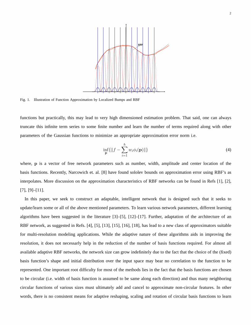
speakingδ(x) is not a function but is a distribution [7]. Further, according to following Lemma such “localized

bumps” can be well-approximated by Gaussian functions (illustrated in Fig. I.):

Lemma 1. Let φ(x) = 1√2π

e−x2

2 andφ(σ)(x) = 1σφ(x

σ ). If Cb(R) denotes the set of continuous, bounded functions

overR), then

∀f ∈ Cb(R), limσ→0

φ(σ) ∗ f(x) = δ(f) (3)

So, theoretically, we can approximate any bounded continuous function with an infinite series of Gaussian

2

��

Fig. 1. Illustration of Function Approximation by Localized Bumps and RBF

functions but practically, this may lead to very high dimensioned estimation problem. That said, one can always

truncate this infinite term series to some finite number and learn the number of terms required along with other

parameters of the Gaussian functions to minimize an appropriate approximation error norm i.e.

infp{‖f −

h∑

i=1

wiφi(p)‖} (4)

where,p is a vector of free network parameters such as number, width, amplitude and center location of the

basis functions. Recently, Narcowich et. al. [8] have found sololev bounds on approximation error using RBF’s as

interpolates. More discussion on the approximation characteristics of RBF networks can be found in Refs [1], [2],

[7], [9]–[11].

In this paper, we seek to construct an adaptable, intelligent network that is designed such that it seeks to

update/learn some or all of the above mentioned parameters. To learn various network parameters, different learning

algorithms have been suggested in the literature [3]–[5], [12]–[17]. Further, adaptation of the architecture of an

RBF network, as suggested in Refs. [4], [5], [13], [15], [16], [18], has lead to a new class of approximators suitable

for multi-resolution modeling applications. While the adaptive nature of these algorithms aids in improving the

resolution, it does not necessarly help in the reduction of the number of basis functions required. For almost all

available adaptive RBF networks, the network size can grow indefinitely due to the fact that the choice of the (fixed)

basis function’s shape and initial distribution over the input space may bear no correlation to the function to be

represented. One important root difficulty for most of the methods lies in the fact that the basis functions are chosen

to be circular (i.e. width of basis function is assumed to be same along each direction) and thus many neighboring

circular functions of various sizes must ultimately add and cancel to approximate non-circular features. In other

words, there is no consistent means for adaptive reshaping, scaling and rotation of circular basis functions to learn

3

from current and past data points. The high degree of redundancy and lack of adaptive reshaping and scaling of

RBF’s are felt to be serious disadvantages of many algorithms and provides the motivation for this paper.

The objectives of this paper are threefold. First, means for reshaping and rotation of Gaussian function are

introduced to learn the local shape and orientation of given data set. The orientation of each radial basis function

is modeled through a rotation parameter vector which, for the two and three dimensional cases can be shown to

be equal to the tangent of the half angle of the principal rotation vector [19]. The shape is captured by solving

independently for the principal axis scale factors. We mention that qualitatively, considering a sharp ridge or canyon

feature in an input-output map, we can expect the principal axes of the local basis functions to approximately align

with the ridge. Secondly, an “Intelligent” adaptation scheme is proposed that learns the optimal shape and orientation

of the basis functions, along with tuning of the centers and widths to enlarge the scope of a single basis function

to approximate as much of the data possible. Thirdly, we modify existing learning algorithms to incorporate the

concept of rotation and re-shaping of the basis functions to enhance their performance. This objective is achieved

by modifying a conventional Modified Resource Allocating Network (MRAN) [4] learning algorithm.

The rest of the paper is structured as follows: In the next section, the notion of rotation and shape optimization

of a Gaussian function in the general case is introduced to alleviate some of the difficulties discussed above. Next,

a novel learning algorithm is presented to learn the rotation parameters along with the parameters that characterize

a regular RBFN. A modification to the MRAN algorithm is suggested to incorporate rotation of the Gaussian

basis functions and finally, the results from various numerical studies are presented to illustrate the efficacy of the

algorithm presented in this paper.

II. D IRECTION DEPENDENTAPPROACH

In this section, we introduce the concept of rotation of generally non-circular radial basis functions that is

motivated through developments in rigid body rotational kinematics [19]. The development is novel because we

believe this represents the first application of the rotation ideas to the function approximation problem. We seek

the optimal center location as well as rotation and shape for the Gaussian basis functions to expand coverage and

approximately capture non-circular local behavior, thereby reducing the total number of basis functions required

for learning.

We propose adoption of the following most generaln-dimensional Gaussian function:

Φi(x, µi, σi, qi) = exp{−12(x− µi)TR−1

i (x− µi)} (5)

Where,R ∈ Rn×n is a fully populatedsymmetric positive definite matrix instead of a diagonal one as in the case of

the conventional Gaussian function representation used in various existing learning algorithms. The assumption of a

4

diagonalR matrix is valid if the variation of output withxj is uncoupled toxk i.e. if different components of input

vector are independent. In this case, the generalized Gaussian function reduces to the product ofn independent

Gaussian functions. However, if the parameters are not independent, there are terms in the resulting output that

depend on off-diagonal terms of the matrix,R. So it becomes useful to learn the off-diagonal terms of the matrix

R for more accurate results (the local basis functions size, shape and orientation can be tailored adaptively to

approximate the local behavior).

Now, using spectral decomposition the matrixR−1 can be written as a product of orthogonal matrices and a

diagonal matrix:

R−1i = CT (qi)S(σi)C(qi) (6)

WhereS is a diagonal matrix containing the eigenvalues,σikof the matrixRi which dictates the spread of the

Gaussian functionΦi andC(qi) is ann × n orthogonal rotation matrix consisting of eigenvectors ofR−1. Now,

it is easy to see that contour plots corresponding to a constant value of a generalized Gaussian function,Φi are

hyperellipsoids inx-space, given by following equation:

(x− µi)TR−1i (x− µi) = c2 (a constant) (7)

Further, substituting for Eq. (6) in Eq. (7), we get an equation for an another hyperellipsoid in a rotated coordinate

system,y = C(x− µ).

[C(qi)(x− µi)]T S(σi) [C(qi)(x− µi)] = yTS(σi)y = c2 (a constant) (8)

From Eq. (8), we conclude that the orthogonal matrix,C represents the rotation of the basis function,Φi. Since the

eigenvectors of the matrixR point in the direction of extreme principal axes of the data set, it naturally follows

that learning the rotation matrix,C is helpful in maximal local trend sensing. ThoughC(qi) is an n × n square

matrix, we require onlyn(n−1)2 parameters to describe it’s most general variation due to the orthogonality constraint

(CTC = I). So, in addition to the parameters that characterize a regular RBFN, we now have to account for the

additional parameters characterizing the orthogonal rotation matrix making a total of(n+2)(n+1)2 parameters for a

minimal parameter description of the most general Gaussian function for ann input single output system. We will

find that the apparent increase in the number of parameters is not usually a cause for concern because the total

number of generalized Gaussian functions required for the representation typically reduces greatly, thereby bringing

down the total number of parameters along with them. also, we will see that the increased accuracy of convergence

provides a powerful argument for this approach. For each RBFN, we require the following parameters:

1) n parameters for the centers of the Gaussian functions i.e.µ.

5

2) n parameters for the spread (shape) of the Gaussian functions i.e.σ.

3) n(n−1)2 parameters for rotation of the principal axis of the Gaussian functions.

4) Weightwi corresponding to the output.

To enforce the positive definiteness and symmetric constraint of matrixR, we propose following three different

parameterizations for the covariance matrix,R.

1) To enforce the orthogonality constraint of the rotation matrix,C, the following result in matrix theory that

is widely used in rotational kinematics namely, the Cayley Transformation [19] is proposed:

Cayley Transformation. If C ∈ Rn×n is any proper orthogonal matrix andQ ∈ Rn×n is a skew-symmetric

matrix then the following transformations hold:

a) Forward Transformations

i) C = (I−Q)(I + Q)−1

ii) C = (I + Q)−1(I−Q)

b) Inverse Transformations

i) Q = (I−C)(I + C)−1

ii) Q = (I + C)−1(I−C)

As any arbitrary proper orthogonal matrixC (or skew-symmetric matrixQ) can be substituted into the above

written transformations, the Cayley Transformations can be used to parameterize the entireO(n) rotational

group by skew symmetric matrices. The forward transformation is always well behaved, however the inverse

transformation encounters a difficulty only near the180◦ rotation wheredet (I + C) → 0. Thus Q is a

unique function ofC except at180◦ rotation andC is always a unique function ofQ. Thus as per the Cayley

transformation, we can parameterize the orthogonal matrixC(qi) in Eq. (6) as:

C(qi) = (I + Qi)−1(I−Qi) (9)

where,qi is a vector of n(n−1)2 distinct elements of a skew symmetric matrixQi i.e. Qi = −QT

i . Note

qi → 0 for C = I and−∞ ≤ qi ≤ ∞ whereqi → ±∞ corresponds to a360◦ rotation about any axis.

Although using the Cayley transformation, the orthogonality constraint on the matrixC can be implicitly

guaranteed, one still needs to check for the positive definiteness ofR by requiringσi > 0.

2) We also introduce the following alternate minimal parameter representation of positive definite matrices that

is motivated by the definition of a correlation matrix normally encountered in the theory of statistics.

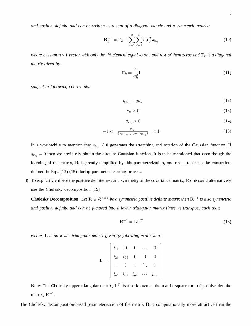
Additive Decomposition. Let R ∈ Rn×n be a symmetric positive definite matrix thenR−1 is also symmetric

6

and positive definite and can be written as a sum of a diagonal matrix and a symmetric matrix:

R−1k = Γk +

n∑

i=1

n∑

j=1

eieTj qkij

(10)

whereei is ann×1 vector with only theith element equal to one and rest of them zeros andΓk is a diagonal

matrix given by:

Γk =1σ2

k

I (11)

subject to following constraints:

qkij= qkji

(12)

σk > 0 (13)

qkii> 0 (14)

−1 <qkij

(σk+qkii)(σk+qkjj

) < 1 (15)

It is worthwhile to mention thatqkij6= 0 generates the stretching and rotation of the Gaussian function. If

qkij= 0 then we obviously obtain the circular Gaussian function. It is to be mentioned that even though the

learning of the matrix,R is greatly simplified by this parameterization, one needs to check the constraints

defined in Eqs. (12)-(15) during parameter learning process.

3) To explicitly enforce the positive definiteness and symmetry of the covariance matrix,R one could alternatively

use the Cholesky decomposition [19]

Cholesky Decomposition.LetR ∈ Rn×n be a symmetric positive definite matrix thenR−1 is also symmetric

and positive definite and can be factored into a lower triangular matrix times its transpose such that:

R−1 = LLT (16)

where,L is an lower triangular matrix given by following expression:

L =

l11 0 0 · · · 0

l21 l22 0 0 0...

......

......

ln1 ln2 ln3 · · · lnn

Note: The Cholesky upper triangular matrix,LT , is also known as the matrix square root of positive definite

matrix, R−1.

The Cholesky decomposition-based parameterization of the matrixR is computationally more attractive than the

7

other two parameterizations because the symmetric and positive definiteness properties ofR−1 are explicitly

enforced in this case to get rid of any kind of constraints. However, to our knowledge, the use of any of the

three above parameterizations for aiding parameter updating in radial basis function approximation applications

is an innovation introduced in this paper. We have experimented with all three approaches and studies to date

favor the Cholesky decomposition mainly because of the programming convenience. Preliminary studies indicate a

significant reduction in the number of basis functions required to accurately model unknown functional behavior

of the actual input output data. In the subsequent sections, we report a novel learning algorithm and a modified

version of the MRAN algorithm to learn this extended set of parameters, we also report the results of application

to five benchmark problems and comparison with existing algorithms.

III. D IRECTED CONNECTIVITY GRAPH

A common main feature of the proposed learning algorithms is a judicious starting choice for the location of the

RBFs via a Directed Connectivity Graph (DCG) approach which allows a priori adaptive sizing of the network for

off-line learning and zeroth order network pruning. Besides this, direction dependent scaling and rotation of basis

functions are initialized for maximal local trend sensing with minimal parameter representations and adaptation of

the network parameters is implemented to account for on-line tuning.

The first step towards obtaining a zeroth order off-line model is the judicious choice of a set of basis functions

and their center locations, followed by proper initialization of the parameters. This exercise is the focus of this

section.

To choose the locations for the RBF centers, we make use of following Lemma that essentially states that “the

center of a Gaussian function is an extremum point”.

Lemma 2. Let Φ(x) : Rn → R represents a Gaussian function i.e.Φ(x) = exp(− (x− µ)T R−1 (x− µ)

)then

x = µ is the only extremum point ofΦ(x) i.e. dΦdx |x=µ = 0. Further, x = µ is the global maximum ofΦ

Thus, from the above-mentioned Lemma, all the interior extremum points of the given surface data should

naturally be the first choice for location of Gaussian functions with theR matrix determined to first order by the

covariance of the data confined in a judicious local mask around a particular extremum point. Therefore, the first step

of the learning algorithm for an RBFN should beto find the extremum points of a given input-output map. It should

be noticed that as the functional expression for the input-output map is unknown, to find the extremum points from

discrete surface data, we need to check the necessary condition that first derivative of the unknown input-output

map should be zero at each and every data point. We mention that the process of checking this condition at every

data point is very tedious and computationally expensive. Hence, we list the following Lemma 3 that provides an

efficient way to find the extremum points of the given input-output map.

8

Lemma 3. Let X be a paracompact space withU = {Uα}α∈A as an open covering andf : X → R be a

continuous function. IfS denotes the set of all extremum points off then there exists a refinement,V = {Vβ}β∈B,

of the open coveringU , such thatS ⊆ W, whereW is the set of the maxima and minima off in open setsVα.

Proof. The proof of this lemma follows from the fact that the input spaceX is a paracompact space as it allow us

to refine any open coverU = {Uα}α∈A of X . Let U = {Uα}α∈A be the open cover of the input spaceX . Further,

assume thatxmaxαandxminα

define the maximum and minimum values off in each open setUα respectively and

W is the set of all such points i.e.card(W) = 2card(A). Now, we know that the set of all local maximum and

minimum points of any function is the same as the setS, of extremum points of that function. Further, w.l.o.g. we

can assume that the set,W, of all local maxima and minima of the function in each open set,Uα, is a subset of

S because if it is not, then we can refine the open coverU further until this is true.

According to the above Lemma 3, for mesh sizes less than a particular value, the setS, of the extremum points

of the unknown input-output mapf , should be subset of the setW, consisting of the relative maxima and minima

of the data points in each grid element. Now, the setS, can be extracted from setW by checking the necessary

condition that first derivative off should be zero at extremum points. This way one need only approximate the

first derivative of the unknown map at2M points, whereM , is the total number of elements in which data has

been divided. It should be noticed thatM is generally much smaller than the total number of data points available

to approximate the unknown input-output map.

Further, to choose the centers from the setS, we construct directed graphsM andN of all the relative maxima

sorted in descending order and all the relative minima sorted in ascending order respectively. We then choose the

points inM andN as candidates for Gaussian function centers with the extreme function value as the corresponding

starting weight of the Gaussian functions. The centers at the points inM andN are introduced recursively until

some convergence criteria is satisfied. The initial value of each local covariance matrixR is computed from

statistical covariance of the data in a local mask around the chosen center. Now, using all the input data, we

adapt the parameters of the chosen Gaussian functions and check the error residuals for the estimation error. If

the error residuals do not satisfy a predefined bound, we choose the next set of points in the directed graphsMandN as center locations for additional Gaussian RBFs and repeat the whole process. The network only grows

in dimensionality when error residuals can not be made sufficiently small, and thus the increased dimensionality

grows incrementally with the introduction of a judiciously shaped and located basis function. The initial location

parameters are simply the starting estimates for the learning algorithm; we show below that the combination of

introducing basis functions sequentially and estimating their shape and location from local data to be highly effective.

9

A. Estimation Algorithm

The heart of any learning algorithm for RBFN is an estimation algorithm to adapt initially defined network

parameters so that approximation errors are reduced to smaller than some specified tolerance. Broadly speaking,

none of the nonlinear optimization algorithms available guarantee the global optimum will be achieved. Estimation

algorithms based on the least squares criteria are the most widely used methods for estimation of the constant

parameter vector from a set of redundant observations. According to the least square criteria, the optimum parameter

value is obtained by minimizing the sum of squares of the vertical offsets (“Residuals”) between the observed and

computed approximations. In general, for nonlinear problems, successive corrections are made based upon local

Taylor series approximations. Further, any estimation algorithm generally falls into the category of Batch Estimator

or Sequential Estimator, depending upon the way in which observation data is processed. A batch estimator processes

the “batch” of data taken from a fixed time-span to estimate the optimum parameter vector while a sequential

estimator is based upon a recursive algorithm, which updates the parameter vector in a recursive manner after

receipt of each observation. Due to their recursive nature, the sequential estimators are preferred for real time

estimation problems, however, batch estimators are usually preferable for offline learning.

To adapt the various parameters of the RBFN as defined in the previous section, we use an extended Kalman

filter [20] for on-line learning while the Levenberg-Marquardt [21], [22] batch estimator is used for off-line learning.

Kalman filtering is a modern (1960) development in the field of estimation [23], [24] though it has its roots as

far back as in Gauss’ work in the1800’s. In the present study, the algebraic version of the Kalman filter is used,

since our model does not involve differential equations. On other hand, Levenberg-Marquardt estimator, being the

combination ofmethod of steepest descentandmethod of differential correction, is a powerful batch estimator tool

in the field of nonlinear least squares [23]. We mention that both the algorithms are very attractive for the problem

at hand and details of both the algorithms can be found in Ref. [23]. Further, for some problems, the Kalman filter

can be used to update the off-line a priori learned network parameters in real time whenever new measurements

are available. The implementation equations for the extended Kalman filter or “Kalman-Schmidt filter” are given in

Table I. To learn the different parameters of the RBFN using any estimation algorithm, the sensitivity (Jacobian)

matrixH needs be computed. The various partial derivatives required to synthesize the sensitivity matrix are outlined

in subsequent subsections for all three parameterizations described in section II:

Cayley Transformation

In this case, the sensitivity matrix,H, can be defined as follows:

H =∂f(x, µ, σ,q)

∂Θ(17)

10

TABLE I

KALMAN -SCHMIDT FILTER

Measurement Model

y = h(xk) + νk

with

E(νk) = 0

E(νlνTk ) = Rkδ(l − k)

Update

Kk = P−k HTk (HkP−k HT

k + Rk)−1

x+k = x−k + Kk(y − Hkx

−k )

P+k = (I − KkH)P−k

where

Hk =∂h(xk)

∂x|x=x−

k

where,f(x, µ,σ,q) =∑N

i=1 wiΦi(µi, σi, qi) andΘ is a N × (n+1)(n+2)2 vector given by:

Θ ={

w1 µ1 σ1 q1 · · · wN µN σN qN

}(18)

Here,q is a n(n−1)2 vector used to parameterize the rank deficient skew-symmetric matrixQ in Eq. (9).

Qij = 0, i = j (19)

= qk i < j

where,k = ‖i− j‖ if i = 1 andk = ‖i− j‖+ ‖i− 1− n‖ for i > 1. Notice that the lower triangular part ofQ

can be formed using the skew-symmetry property ofQ. The partial derivatives required for the computation of the

sensitivity matrix,H are computed using Eqs. (5), (6) and (9), as follows:

∂f

∂wk= φk (20)

∂f

∂µk

=[wkφkR−1

k (x− µk)]T

(21)

∂f

∂σki

= wkφky2

i

σ3ki

,yi = Ck(x− µk), i = 1 . . . n (22)

∂f

∂qkl

= −wk

2φk

[(x− µk)

T ∂CTk

∂qkl

SkCk(x− µk) + (x− µk)TCT

k Sk∂Ck

∂qkl

(x− µk)]

,

l = 1 . . . n(n− 1)/2 (23)

11

Further, the partial∂CTk

∂qkl

in Eq. (23) can be computed by substituting forC from Eq. (9):

∂Ck

∂qkl

=∂

∂qkl

(I + Qk)−1 (I−Qk) + (I + Qk)

−1 ∂

∂qkl

(I−Qk) (24)

Making use of the fact that(I + Q)−1 (I + Q) = I, we get:

∂

∂qkl

(I + Qk)−1 = − (I + Qk)

−1 ∂Qk

∂qkl

(I + Qk)−1 (25)

substitution of Eq. (25) in Eq. (24) gives:

∂Ck

∂qkl

= − (I + Qk)−1 ∂Qk

∂qkl

(I + Qk)−1 (I−Qk)− (I + Qk)

−1 ∂Qk

∂qkl

(26)

Now, Eqs. (20)-(23) constitute the sensitivity matrixH for the Extended Kalman Filter. We mention that although

Eq. (6) provides a minimal parameterization of the matrixR, we need to make sure that the scaling parameters

denoted byσi are always greater than zero. So in case of any violation of this constraint, we need to invoke

the parameter projection method to project inadmissible parameters into the set they belong to, thereby ensuring

that the matrixR remains symmetric and positive definite at all times. Further, based on our experience with

this parameterization, it is highly nonlinear in nature and sometimes causes problems with the convergence of the

estimation algorithm. We found that this difficulty is alleviated by considering the two alternate representations,

discussed earlier. We summarize the sensitivity matrices for these alternate parameterizations in the next subsections.

Additive Decomposition of the “Covariance” Matrix,R

Using the additive decomposition for theRi matrix in Eq. (5) the different partial derivatives required for

synthesizing the sensitivity matrixH can be computed by defining the following parameter vectorΘ

Θ ={

w1 µ1 σ1 q1 · · · wN µN σN qN

}(27)

The required partials are then given as follows:

∂f

∂wk= φk (28)

∂f

∂µk

=[wkφkP−1

k (x− µk)]T

(29)

∂f

∂σki

= wkφk(xi − µki

)2

σ3ki

, i = 1 . . . n (30)

∂f

∂qkl

= −wkφk(xi − µki)T (xj − µkj

), l = 1 . . . n(n + 1)\2, i, j = 1 . . . n. (31)

Thus, Eqs. (28)-(31) constitute the sensitivity matrixH. It is to be mentioned that even though the synthesis of

the sensitivity matrix is greatly simplified, one needs to check the constraint satisfaction defined in Eqs. (12)-(15)

12

at every update. In case these constraints are violated, we once again invoke the parameter projection method to

project the parameters normal to the constraint surface to nearest point on the set they belong to, thereby ensuring

that the covariance matrix remains symmetric and positive definite at all times.

Cholesky Decomposition of “Covariance” Matrix,R

Like in previous two cases, once again the sensitivity matrix,H, can be computed by defining the parameter

vector,Θ, as:

Θ ={

w1 µ1 l1 · · · wn µn ln}

(32)

where,li is the vector of elements parameterizing the lower triangular matrix,L.

Carrying out the algebra the required partials can be computed as:

∂f

∂wk= φk (33)

∂f

∂µk=

[wkφkR−1

k (x− µk)]T

(34)

∂f

∂lkl

= −wk

2φk

[(x− µk)T

(∂Lk

∂lkl

LTk + Lk

∂LTk

∂lkl

)(x− µk)

],

l = 1 . . . n(n− 1)\2 (35)

Further,Lk can be written as:

Lk =n∑

i=1

n∑

j=i

eiejLkij(36)

Therefore,∂Lk

∂lkl

can be computed as:

∂Lk

∂lkl

=n∑

i=1

n∑

j=i

eiej (37)

Thus, Eqs. (33)-(35) constitute the sensitivity matrixH. It is to be mentioned that unlike the Cayley transformation

and the Additive decomposition, Cholesky decomposition guarantees the symmetry and positive definiteness of

matrix, R, without any additional constraints and so is more attractive for learning the matrix,R.

It should be noted that although these partial derivatives are computed to synthesize the sensitivity matrix for

the extended Kalman filter they are required in any case, even if a different parameter estimation algorithm is used

(the computation of these sensitivity partials is inevitable).

Finally, the various steps for implementing the Directed Connectivity Graph Learning Algorithm are summarized

as follows:

Step 1 Find the interior extremum points i.e. global maximum and minimum of the given input-output data.

Step 2 Grid the given input space,X ∈ Rn using hypercubes of lengthl.

13

Step 3 Find the relative maximum and minimum of given input-output data on the grid points in the region

covered by each hypercube.

Step 4 Make a directed graph of all maximum and minimum points sorted in descending and ascending order

respectively. Denote the directed graph of maximum points and minimum points byM andN .

Step 5 Choose first point from graphsM andN , denoted byxM and xN repectively, as candidates for

Gaussian center and respective function values as the initial weight estimate of those Gaussian functions

because at center the Gaussian function response is1.

Step 6 Evaluate initial covariance matrix estimate,R, using the observations in a local mask around points

xM andxN .

Step 7 Parameterize the covariance matrix,R, using one of the parameterizations defined in section II.

Step 8 Use the Extended Kalman filter (Table I) or the Levenberg-Marquardt algorithm to refine the parameters

of the network using the given input-output data.

Step 9 On each iteration, use parameter projection to enforce parametric constraints, if any, depending upon

the covariance matrix decomposition.

Step 10 Check the estimation error residuals. If they do not satisfy the prescribed accuracy tolerance then

choose the next point in the directed graphsM andN as the Gaussian center and restart at step5.

Grid generation in step2 is computationally costly, unless careful attention is paid to efficiency. To grid the

input spaceX ∈ Rn, in a computationally efficient way, we designate a unique cell number to each input point

in N th decimal system, depending upon its coordinates inRn. Here,N = max{N1, N2, · · · , Nn} andNi denotes

the number of cells required alongith direction. The pseudo-code for the grid generation is given below:

Psuedo-Code For Grid Generation.

for ct = 1 : n

xlower(ct) = min(inputdata(:, ct))

xupper(ct) = max(inputdata(:, ct))

end

deltax=(xupper-xlower)/N

for ct = 1 : Npoints

cellnum(ct) = ceil((inputdata(ct, :)− xlower)./deltax)

cellIndex(ct) = getindex(cellnum(ct))

end

The relative maxima and minima in each cell are calculated by using all the data points with the same cell

14

number. Though this process of finding the centers and evaluating the local covariance followed by the function

evaluation with adaptation and learning seems computationally extensive, it helps in reducing the total number of

Gaussian functions and therefore keeps the “curse of dimensionality” in check. Further, the rotation parameters and

shape optimization of the Gaussian functions enables us to approximate the local function behavior with improved

accuracy. Since we use the Kalman filter to refine the parameters of the RBF network, the selection of starting

estimates for the centers can be made off-line with some training data and the same algorithm can be invoked online

to adapt the parameters of the off-line network. Obviously, we can choose to constrain any subset of the network

parameters, if necessary, to reduce dimensionality. Any new Gaussian centers can be added to the existing network

depending upon the statistical information of the approximation errors. Additional localization and reduction in the

computational burden can be achieved by exploiting the local dominance near a given point on only a small subset

of RBFN parameters.

IV. M ODIFIED M INIMAL RESOURCEALLOCATING ALGORITHM (MMRAN)

In this section, we will illustrate how the rotation parameters can be incorporated in the existing RBF learning

algorithms by modifying the popular Minimal Resource Allocating Network (MRAN). To show the effectiveness

of this modification, we include the rotation parameters also as adaptable parameters while keeping the same center

selection and pruning strategy as in the conventional MRAN. For sake of completion, we give a brief introduction

to MRAN and the reader should refer to Ref. [4] for more details (note that, MRAN is an improvement of the

Resource Allocating Network (RAN) of Platt [16]). It adopts the basic idea of adaptively growing the number

of radial basis functions and augments it with a pruning strategy to eliminate little-needed radial basis functions

(those with weights smaller than some tolerance) with the goal of finding a minimal RBF network. RAN allocates

new units as well as adjusts the network parameters to reflect the complexity of function being approximated.

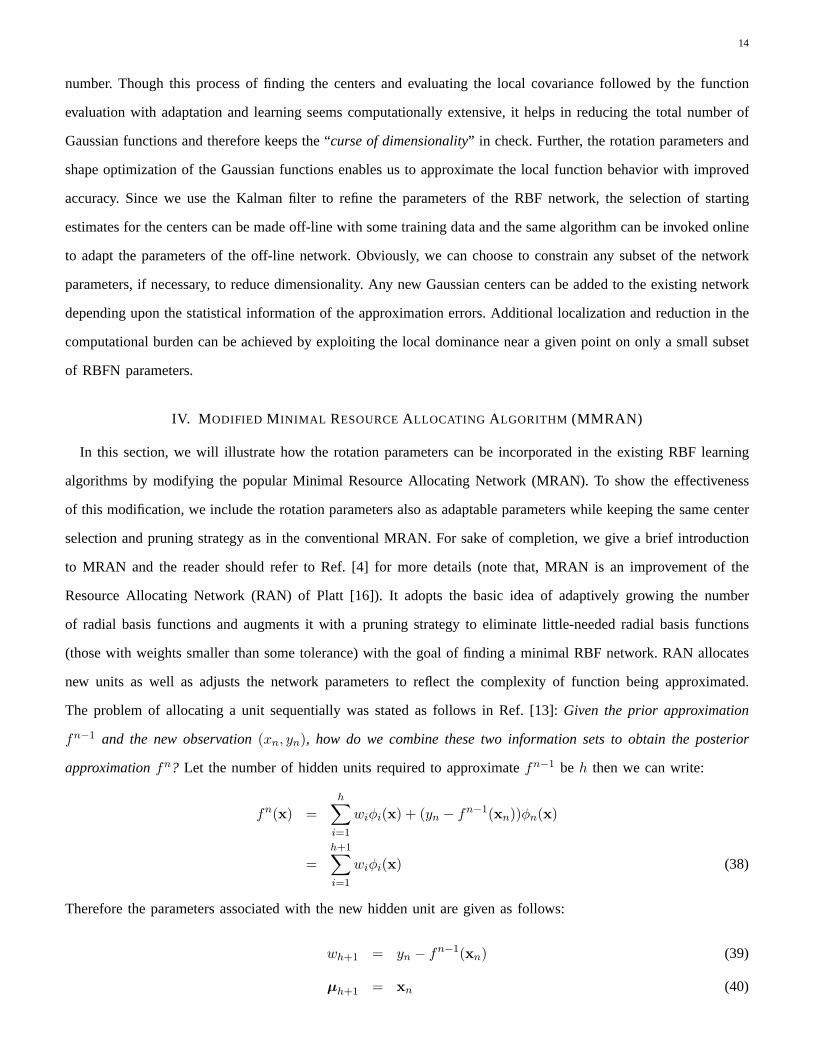
The problem of allocating a unit sequentially was stated as follows in Ref. [13]:Given the prior approximation

fn−1 and the new observation(xn, yn), how do we combine these two information sets to obtain the posterior

approximationfn? Let the number of hidden units required to approximatefn−1 be h then we can write:

fn(x) =h∑

i=1

wiφi(x) + (yn − fn−1(xn))φn(x)

=h+1∑

i=1

wiφi(x) (38)

Therefore the parameters associated with the new hidden unit are given as follows:

wh+1 = yn − fn−1(xn) (39)

µh+1 = xn (40)

15

σh+1 = σn (41)

Heuristically, the estimated width of new Gaussian function,σn, will be proportional to the shortest distance between

xn and the existing centers i.e.

σn = κ‖xn − µnearest‖ (42)

κ should be chosen judiciously to account for the amount of overlap between different Gaussian functions.

The main difficulty with this kind of approach is that we may go on adding new hidden units that contribute

little to the final estimate. Therefore, a new hidden unit is added to existing network only if it satisfies following

criteria [16]:

‖xi − µnearest‖ > ε (43)

‖ei‖ = ‖yi − f(xi)‖ > emin (44)

ermsi =

√√√√i∑

j=i−(Nw−1)

‖ej‖2

Nw> ermin

(45)

Eq. (43) ensures that a new node is added if it is sufficiently far from all the existing nodes. Eq. (44) decides

whether existing nodes meet the error specification or not. Eq. (45) takes care of noise in the observations by

checking the sum squared error for pastNw observations.ε, emin anderminare different thresholds which should

be chosen appropriately.

If the above-mentioned criteria are not met then the following network parameters are updated using the gradient

descent approach or extended Kalman filter as suggested by Sundararajan [4].

Θ ={

w1 µT1 σ1 · · · wh µT

h σh

}(46)

It should be noted that like most other available RBFN learning algorithms MRAN also assumes the Gaussian

functions to be circular in nature. To eliminate this assumption in the present study, we augment the parameter

vector with a rotation parameter vector,q and different spread parameters,σikas described in section II.

Θ ={

w1 µT1 σ1 q · · · wh µT

h σh q}

(47)

Whenever a new node or Gaussian function is added to the MMRAN network, the corresponding rotation parameters

are first set to zero and the spread parameters along different directions are assumed to be equal i.e. initially, the

Gaussian functions are assumed to be circular.

The last step of the MRAN algorithm is the pruning strategy as proposed in Ref. [4]. The basic idea of the

pruning strategy is to prune those nodes that contribute less than a predetermined number,δ, for Sw consecutive

16

observations. Finally, the modified MRAN algorithm (MMRAN) can be summarized as follow:

Step 1 Compute the RBF network output using following equation:

y =h∑

i=1

wiΦi(x,Θ) (48)

Φi(x,Θ) = exp(−1

2(x− µi)TR−1(x− µi)

)(49)

Step 2 Compute different error criteria as defined in Eqs. (43)-(44).

Step 3 If all the error criteria hold then create a new RBF center with different network parameters assigned

according to following Eqs.:

wh+1 = ei (50)

µh+1 = xi (51)

σh+1k= κ‖xi − µnearest‖, ∀k = 1, 2, · · · , n (52)

q = 0 (53)

Step 4 If criteria for adding a new node to network are not met then update different parameters of the network

using EKF as described in section III-A.

Step 5 Remove those nodes of the RBF network that contribute little to the output of the network for a certain

number of consecutive observations.

V. NUMERICAL SIMULATIONS AND RESULTS

The advantages of rotation and re-shaping the Gaussian basis functions are evaluated by implementing the DCG

and modified MRAN algorithm using a variety of test examples in the areas of function approximation, chaotic

time series prediction and dynamical system identification problems. Most of the test case examples are either taken

from the open literature or from the recently set up data modeling benchmark group [25] by IEEE Neural Network

Council. In this section, we provide a comprehensive comparison of DCG and modified MRAN algorithm with

various other conventional learning algorithms. At same time, these results also, demonstrate that the inclusion of

rotation and re-shaping parameters significantly enhances the performance of the MRAN algorithm, for all five test

problems.

17

02

46

810

0

5

100

2

4

6

8

10

12

x1

x2

f(x,

y)

(a) True Surface Plot

0 2 4 6 8 100

1

2

3

4

5

6

7

8

9

10

x1

x 2

(b) True Contour Plots

Fig. 2. True Surface and Contour Plots For Test Example1

A. Test Example1: Function Approximation

The first Test Example for the function approximation is constructed by using the following analytic surface

function [26].

f(x1, x2) =10

(x2 − x21)2 + (1− x1)2 + 1

+5

(x2 − 8)2 + (5− x1)2 + 1+

5(x2 − 8)2 + (8− x1)2 + 1

(54)

Figures 2(a) and 2(b) show the true surface and contour plots of the above functional expression respectively.

According to our experience, this particular function has many important features including the sharp ridge that

is very difficult to learn accurately with existing function approximation algorithms with a reasonable number of

nodes. To approximate the function given by Eq. (54), a training data set is generated by taking10, 000 uniform

random sampling in the interval[0-10]× [0-10] in theX1-X2 space while test data consists of5, 000 other uniform

samples of the interval[0-10]× [0-10].

To show the effectiveness of the rotation of Gaussian basis functions, we first use the standard MRAN algorithm

without rotation parameters, as discussed in Ref. [4]. Since the performance of MRAN algorithm depends upon the

choice of various tuning parameters, several simulations were performed for various values of the tuning parameters

before selecting the tuning parameters (given in Table II) which gives us the smallest approximation error. Figs.

4(a) and 4(b) show the approximation error for the training data set and the evolution of the number of centers

with number of data points. From these figures, it is clear that approximation errors are quite high even for the

training data set an even though the number of Gaussian functions settled down to70 approximately after3000

data points. Further, Figs. 4(c) and 4(d) show the approximated test surface and contours plots respectively, whereas

Figs 4(e) and 4(f) show the percentage error surface and error contour plots corresponding to test data respectively.

From these figures, it is apparent that approximation errors are pretty large (≈ 15%) along the knife edge of the

sharp ridge line while they are< 1% in other regions. Actually, this is also the reason for the high value of the

18

standard deviation of the approximation error for MRAN in Table III, the errors along the sharp ridge dominate

the statistics. The failure of MRAN type learning algorithms in this case can be attributed directly to theinability

of the prescribed circular Gaussian basis functionto approximate the sharp ridge efficiently.

TABLE II

VARIOUS TUNING PARAMETERS FORMRAN AND MODIFIED MRAN A LGORITHMS

Algorithm εmax εmin γ emin erminκ p0 q0 R Nw Sw δ

Std. MRAN 3 1 0.66 2× 10−3 15× 10−3 0.45 10−1 10−3 10−5 200 500 5× 10−3

Modified MRAN 3 1.65 0.66 2× 10−3 15× 10−3 0.45 10−1 10−3 10−5 200 500 5× 10−3

Further, to show the effectiveness of the shape and rotation parameters, we modify the MRAN algorithm, as

discussed in section IV, by simply including the shape and rotation parameters also as adaptable while keeping

the same center selection and pruning strategy. The modified MRAN algorithm is trained and tested with the same

training data set that we used for the original algorithm. In this case too, a judicious selection of various tuning

parameter is made by performing a few different preliminary simulations and selecting final tuning parameters

(given in Table II) which give us a near-minimum approximation error. Figs. 5(a) and 5(b) show the approximation

error for the training data set and the evolution of number of centers with the number of data points.From these

figures, it is clear that by learning the rotation parameters, the approximation errors for the training data set is

reduced by an almost order of magnitude whereas the number of Gaussian functions is reduced to half. It should

be noted, however, that∼ 50% reduction in number of Gaussian functions corresponds to only a17% reduction in

the number of network parameters to be learned. Figs. 5(c) and 5(d) show the approximated surface and contours

plots respectively whereas Figs 5(e) and 5(f) show the percentage error surface and error contour plots respectively.

As suspected, the approximation errors are significantly reduced (≈ 5%) along the knife edge of the sharp ridge

line while they are still< 1% in other regions. From Table III, it is apparent that the mean and standard deviation

of the approximation errors are also reduced very significantly.

Finally, the DCG algorithm, proposed in section III, is used to approximate the analytical function given by Eq.

(54). As mentioned in section III, we first divide the whole input region into a total of16 square regions (4 × 4

cells); this decision was our first trial, better results might be obtained by tuning. Then we generated a directed

connectivity graph of the local maxima and minima in each sub-region that finally lead to locating and shaping

the24 radial basis functions that, after parameter optimization gave approximation errors less than5%. This whole

procedure is illustrated in Fig. 3. The DCG algorithm is also trained and tested with the same data set that we use

19

(a) Step1: Locate Interior Extremum Points

��

��

(b) Step2: Locate extremum points along the boundary ofinput Space

��

��

��

��

��

��

(c) Step3: Divide the input space into smaller sub-regionsand locate local extremum points in each sub-region

��

��

��

��

��

��

��

��

(d) Step 4: Make a directed connectivity graph (open) oflocal maxima and minima and use local masks to computecovariance

Fig. 3. Illustration of Center Selection in DCG Network

for the MRAN algorithm training and testing. Figs. 6(a) and 6(b) show the estimated surface and contour plots

respectively for the test data. From these figures, it is clear that we are able to learn the analytical function given

in Eq. (54) very well. In Fig. 6(b) the circular (◦) and asterisk (∗) marks denote the initial and final positions

(after learning process is over) of the Gaussian centers. As expected, initially the center locations cover the global

and local extremum points of the surface and finally some of those centers, shape and rotation parameters move a

significantly. The optimum location, shape, and orientation of those functions along the sharp ridge are critical to

learn the surface accurately with a small number of basis functins. Figs. 6(c) and 6(d) show the error surface and

error contour plots for the DCG approximated function. From Fig. 6(c), it is clear that approximation errors are

less than5% whereas from Fig. 6(d) it is clear that even though we have approximated the sharp surface very well,

the largest approximation errors are still confined to the vicinity of the ridge. Clearly, we can continue introducing

local functions along the ridge until the residual errors are declared small enough. Already, however, advantages

relative to competing methods are quite evident.

20

TABLE III

COMPARATIVE RESULTS FORTEST EXAMPLE 1

Algorithm Mean Error Std. Deviation (σ) Max. Error Number of Network Parameters

Std. MRAN 32× 10−4 0.1811 2.0542 280

Modified MRAN 6.02× 10−4 0.0603 0.7380 232

DCG 5.14× 10−4 0.0515 0.5475 144

For comparison sake, the mean approximation error, standard deviation of approximation error and total number

of network parameters learned are listed in Table III for MRAN (with and without rotation parameters) and DCG

algorithms. From these numbers, it is very clear that the mean approximation error and standard deviation decreases

by factors from three to five if we include the rotation and shape parameters. Further, this reduction is also

accompanied by a considerable decrease in number of learned parameters required to define the RBFN network

in each case. It should be mentioned that the improvement in performance of the modified MRAN algorithm over

the standard MRAN can be attributed directly to theinclusion of shape and rotation parameters, because the other

parameter selections and learning criteria for the modified MRAN algorithm are held the same as for the original

MRAN algorithm. Although, there is not much difference between the modified MRAN and DCG algorithm results,

in terms of accuracy, in the case of the DCG algorithm, a total of only144 network parameters are required to be

learned as compared to232 in case of the modified MRAN. This33% decrease in number of network parameters to

be learned in the case of the DCG can be attributed to thejudicious selection of centers, using the graph of maxima

and minima, and the avoidance of local convergence to sub-optimal value of the parameters. It is anticipated that

persistent optimization and pruning of the modified MRAN may lead to results comparable to the DCG results. In

essence DCG provides more nearly the global optimal location, shape and orientation parameters for the Gaussian

basis functions to start the modified MRAN algorithm.

B. Test Example2: 3 Input- 1 Output Continuous Function Approximation

In this section, the effectiveness of the shape and rotation parameters is shown by comparing the modified MRAN

and DCG algorithms withDependence Identification(DI) algorithm [27]. The DI algorithm bears resemblance to

the boolean network construction algorithms and it transforms the network training problem into a set of quadratic

optimization problems that are solved by number of linear equations. The particular test example considered here is

21

0 2000 4000 6000 8000 10000−2

−1.5

−1

−0.5

0

0.5

1

1.5

2

Number of Data Points

App

roxi

mat

ion

Err

or

(a) Training Data Set Error Plot

0 2000 4000 6000 8000 100000

10

20

30

40

50

60

70

80


Num

ber

of C

ente

rs

(b) Number of RBFs vs Number of Data Points

0

2

4

6

8

10

0

2

4

6

8

100

1

2

3

4

5

6

7

8

9

10

xy

z

(c) Estimated Surface Plot

x

y

0 2 4 6 8 100

2

4

6

8

10

(d) Estimated Contour Plots

0

5

10

0

5

10−20

−10

0

10

20

xy

App

roxi

mat

ion

Err

or (

%)

(e) Approximation Error Surface (%) Plot

x

y

0 2 4 6 8 100

2

4

6

8

10

(f) Approximation Error Contour Plots

Fig. 4. MRAN Approximation Results For Test Example1

borrowed from Ref. [27] and involves the approximation of a highly nonlinear function given by following equation:

y =110

(ex1 + x2x3 cos(x1x2) + x1x3) (55)

Here,x1 ∈ [0, 1] andx2, x3 ∈ [−2, 2]. We mention that in Ref. [4], Sundarajan et. al. compared MRAN algorithm

with DI algorithm. Like in Ref. [4], [27], the input vector for MMRAN and DCG isx ={

x1 x2 x3

}T

and

the training data set for network learning is generated by taking2000 uniformly distributed random values of the

input vector and calculating the associated value ofy according to Eq. (55). The different tuning parameters for

the MMRAN algorithm are given in Table IV. Fig. 7(a) shows the growth of the modified MRAN network. In

22

0 2000 4000 6000 8000 10000−0.6

−0.4

−0.2

0

0.2

0.4

0.6

0.8


App

roxi

mat

ion

Err

or

(a) Training Data Set Error Plot

0 2000 4000 6000 8000 100000

5

10

15

20

25

30

35

40


Num

ber

of C

ente

rs

(b) Number of RBFs vs Number of Data Points

0

5

10

0

5

100

5

10

xy

z

(c) Estimated Surface Plot

x

y0 2 4 6 8 10

0

2

4

6

8

10

(d) Estimated Contour Plots

0

5

10

0

5

10−5

0

5

10

xy

App

roxi

mat

ion

Err

or (

%)

(e) Approximation Error Surface (%) Plot

x1

x 2

0 2 4 6 8 100

2

4

6

8

10

(f) Approximation Error Contour Plots

Fig. 5. Modified MRAN Approximation Results For Test Example1

case of the DCG network, the whole input space is divided into2× 2× 2 grid so giving us a freedom to choose

the connectivity graph of16 centers. However, finally we settled down to a total4 basis functions to have mean

training data set errors of the order of10−3. Further, Fig. 7 shows the result of testing the modified MRAN and

DCG network with the input vectorx set to following three parameterized functions oft as described in Ref. [4],

23

02

46

810

02

46

810

0

2

4

6

8

10

xy

(a) Estimated Surface Plot

0 2 4 6 8 100

1

2

3

4

5

6

7

8

9

10

x1

x 2

(b) Estimated Contour Plots

02

46

810

0

2

4

6

8

10−6

−4

−2

0

2

4

6

xy

(c) Approximation Error Surface (%) Plot

x0 1 2 3 4 5 6 7 8 9 10

0

1

2

3

4

5

6

7

8

9

10

(d) Approximation Error Contour Plots

Fig. 6. DCG Simulation Results For Test Example1

TABLE IV

VARIOUS TUNING PARAMETERS FORMODIFIED MRAN A LGORITHM FOR TEST EXAMPLE 2


Modified MRAN 3 0.3 0.97 2× 10−3 12× 10−2 0.70 1 10−1 0 100 2000 1× 10−4

[27].

Test Case1

x1(t) = t

x2(t) = 1.61

x3(t) =

8t− 2 0 ≤ t < 12

−8t + 6 12 ≤ t < 1

(56)

24

Test Case2

x1(t) = t

x2(t) =

8t− 2 0 ≤ t < 12

−8t + 6 12 ≤ t < 1

x3(t) = step(t)− 2step(t− 0.25) + 2step(t− 0.5)− · · ·

(57)

Test Case3

x1(t) = t

x2(t) = step(t)− 2step(t− 0.25) + 2step(t− 0.5)− · · ·x3(t) = 2 sin(4πt)

(58)

(59)

As in Ref. [4], [27], in all 3 test casest takes on100 evenly spaced values in the[0, 1] interval. In Table V,

comparison results are shown in terms of percentage squared error for each test case and network parameters. The

performance numbers for MRAN and DI algorithms are taken from Ref. [4]. From this Table and Fig. 7, it is clear

that modified MRAN and DCG achieve smaller approximation error with a small number of network parameters.

Once again, the effectiveness of the shape and rotation parameters is clear from the performance difference between

standard MRAN and modified MRAN algorithm, although the advantage is not as dramatic advantage as the first

example.

TABLE V

COMPARATIVE RESULTS FOR3-INPUT, 1-OUTPUT NONLINEAR FUNCTION CASE

Algorithm NetworkArchitecture

Squared PercentageError for all TestingSets

Number of Net-work Parameters

Modified MRAN 3-4-1 0.0265 40

DCG 3-4-1 0.0237 40

Std. MRAN 3-9-1 0.0274 45

DI 4-280-1 0.0295 1400

25

0 200 400 600 800 1000 1200 1400 1600 1800 20000

0.5

1

1.5

2

2.5

3

3.5

4

4.5

5


Num

ber

of C

ente

rs

(a) Network Growth for Modified MRAN Al-gorithm

0 0.1 0.2 0.3 0.4 0.5 0.6 0.7 0.8 0.9 1−0.3

−0.2

−0.1

0

0.1

0.2

0.3

0.4

0.5

t

Net

wor

k O

utpu

t

True Test DataModified MRANdata3

(b) Test Case 1

0 0.1 0.2 0.3 0.4 0.5 0.6 0.7 0.8 0.9 1−0.1

−0.05

0

0.05

0.1

0.15

0.2

0.25

0.3

0.35

0.4

t

Net

wor

k O

utpu

t

True Test DataModified MRANDCG

(c) Test Case2

0 0.1 0.2 0.3 0.4 0.5 0.6 0.7 0.8 0.9 10.1

0.15

0.2

0.25

0.3

0.35

0.4

0.45

0.5

t

Net

wor

k O

utpu

t

True Test DataModified MRANDCG

(d) Test Case3

Fig. 7. Simulation Results For Test Example2

C. Test Example3: Dynamical System Identification

In this section, a nonlinear system identification problem is considered to test the effectiveness of the shape and

rotation parameters. The nonlinear dynamical system is described by the following equation and is borrowed from

Ref. [4], [28]

yn+1 =1.5yn

1 + y2n

+ 0.3 cos yn + 1.2un (60)

The particular system considered, here, was originally proposed by Tan et. al. in Ref. [28]. In Ref. [28], a recursive

RBF structure with fixed42 neurons and one width value(0.6391) is used to identify the discrete-time dynamical

system given by Eq. (60). Further, in Ref. [4] the standard MRAN algorithm is employed to predict the value of

y(n + 1) with 11 hidden units. It should be noticed that while the number of hidden units reduced by a factor of

three, but total number of parameters (44 in case of MRAN) to be learned have increased by2 as compared to

total number of parameters learned in Ref. [28].

Like in the previous test examples, to show the effectiveness of shape and rotation parameters, we first use the

modified MRAN algorithm to identify the particular discrete-time system. Like in Refs. [4], [28], the RBF network

is trained by taking200 uniformly distributed random samples of input signals,un, between−2 and2. The network

26

input vector,x, is assumed to consist ofyn−1, andun, i.e.

x ={

yn−1 un

}(61)

To test the learned RBF network, test data is generated by exciting the nonlinear system by a sequence of periodic

inputs [4], [28]:

u(n) =

sin(2πn/250) 0 < n ≤ 500

0.8 sin(2πn/250) + 0.2 sin(2πn/25) n > 500(62)

The different tuning parameters for modified MRAN algorithms are given in Table VI. Fig. 8(a) shows the plot of

actual system excitation, the RBF network output learned by modified MRAN algorithm with shape and rotation

parameters and the approximation error. Fig. 8(b) shows the plot of the evolution of RBF network with number of

data points. From, these plots, we can conclude that number of hidden units required to identify the discrete-time

system accurately reduces to7 from 11 if we introduce shape and rotation optimization of the Gaussian functions

in the standard MRAN algorithm. However, in terms of the total number of learning parameters there is a reduction

of 2 parameters when we include the shape and rotation parameters in the MRAN algorithm.

Finally, the Directed Connectivity Graph Learning Algorithm is used to learn the unknown nonlinear behavior

of the system described by Eq. (60). For approximation purposes, the input space is divided into2× 2 grid giving

us a freedom to choose maximum8 radial basis functions. However, the final network structure requires only6

neurons to have approximation errors less than5%. Figure 8(c) shows the plot of training data set approximation

error with 6 basis functions while Figure 8(d) shows the actual system excitation for test data, the RBF network

output learned by the DCG algorithm and the approximation error. From these plots, we can conclude that the

DCG algorithm is by far the most advantageous since it requires only6 Gaussian centers to learn the behavior of

the system accurately as compared to42 and11 Gaussian centers used in Refs. [28] and [4] respectively. In terms

of the total number of learning parameters, the DCG algorithm is also preferable. For DCG, we need to learn only

6 × 6 = 36 parameters as compared to42 and 44 parameters for MMRAN and MRAN respectively. This result,

once again reiterates our observation that the better performance of DCG and MMRAN algorithm can be attributed

to the adaptive shape and rotation learning of the Gaussian functions as well as thejudicious choice of initial

centers (in case of DCG). It is obvious we achieve(i) more accurate convergence(ii) fewer basis functions, and

(iii) fewer network parameters, and, we have a systematic method for obtaining the starting estimates.

27

TABLE VI



Modified MRAN 3 1 0.6 0.04 0.4 0.50 1 0 10−2 25 200 10−4

0 100 200 300 400 500 600 700 800 900 1000−3

−2

−1

0

1

2

3


Desired Output

Modified MRAN

Output Error

(a) Test Data Approximation Result for modi-fied MRAN Algorithm

0 20 40 60 80 100 120 140 160 180 2000

1

2

3

4

5

6

7

Number of Data PointsN

umbe

r of

Cen

ters

(b) Number of Centers vs Data Points

0 20 40 60 80 100 120 140 160 180 200−2.5

−2

−1.5

−1

−0.5

0

0.5

1

1.5

2

2.5


App

roxi

mat

ion

Err

or

(c) Training Set Approximation Error for DCGAlgorithm

0 100 200 300 400 500 600 700 800 900 1000−3

−2

−1

0

1

2

3


Desired Output

DCG Output

Output Error

(d) Test Data Approximation Result for DCGAlgorithm


D. Test Example4: Chaotic Time Series Prediction Problem

The effectiveness of shape and rotation parameters has also been tested with the chaotic time series generated

by Mackey-Glass time delay differential equation [29]:

ds(t)dt

= −βs(t) + αs(t− τ)

1 + s10(t− τ)(63)

This equation is extensively studied in Refs. [4], [16], [30], [31] for its chaotic behavior and is listed as one of the

benchmark problems at IEEE Neural Network Council web-site [25]. Like in previous studies [4], [16], [30], [31],

28

the various parameters were set toα = 0.2, β = 0.1, τ = 17 ands(0) = 1.2. Further, to generate the training and

testing data set, the time series Eq. (63) is integrated by using the fourth-order Runge-Kutta method to find the

numerical solution. This data set can be found in the file mgdata.dat belonging to the FUZZY LOGIC TOOLBOX

OF MATLAB 7 and at IEEE Neural Network Council web-site.

Once again, to study the effectiveness of introducing shape and rotation parameters only, we used modified

MRAN algorithm and DCG algorithm to perform a short-term prediction of this chaotic time series. We predict the

value ofs(t+6) from the current values(t) and the past valuess(t− 6), s(t− 12) ands(t− 18). Like in previous

studies [4], [16], [30], [31], the first500 data-set values are used for network training while the remaining500

values are used for testing purposes. The different tuning parameters for the modified MRAN algorithm are given

in Table VII. For the DCG approximation purposes, the input space is divided into2 × 2 × 2 × 2 grid giving us

freedom to choose a maximum of32 radial basis functions. However, the final network structure required only4

neurons that result in approximation errors less than5%. We mention that due to the availability of small number

of training data set examples, we used the Levenberg-Marquardt [23] algorithm to optimize the DCG network.

Fig. 9(a) shows the MMRAN network growth with the number of training data set examples while Figs. 9(b)

and 9(c) show the plots for approximated test data and approximation test data error respectively. From these plots,

we can conclude that the MMRAN algorithm requires only6 Gaussian centers to learn the behavior of the system

accurately as compared to29 and 81 Gaussian centers used in Refs. [4] and [16] respectively. In terms of the

total number of learning parameters too, the MMRAN algorithm is preferable as compared to MRAN and RAN.

For MMRAN algorithm, we need to learn only6 × 15 = 90 parameters as compared to174 parameters required

for MRAN algorithm. In case of DCG, the number of Gaussian centers required was reduced further down to

only 4 while the total number of learned parameters reduced to60 as compared to90 in case of the MMRAN

algorithm and174 for the standard MRAN algorithm. In Ref. [31], TableIX compares the various algorithms

presented in the literature in terms of their root mean squared error (RMSE) for this particular problem. Here, in

Table VIII, we present comparison results for MMRAN, DCG and many other algorithms. The direct comparison of

MRAN and MMRAN results reveals the fact that inclusion of the shape and rotation parameters greatly enhance the

approximation accuracy while significantly reducing the number of parameters required to define the RBF network

for a particular algorithm. It should be also noted that both the DCG and MMRAN algorithm performed very well

as compared to all other algorithms for this particular example, in terms of both smallness of the RMS error and

the number of free network parameters.

29

TABLE VII



Modified MRAN 2 0.5 0.66 10−5 10−4 0.27 1 0 10−1 100 1000 10−4

0 50 100 150 200 250 300 350 400 450 5000

1

2

3

4

5

6


Num

ber

of C

ente

rs

(a) Number of Centers vs Data Points

0 50 100 150 200 250 300 350 400 450 5000.4

0.5

0.6

0.7

0.8

0.9

1

1.1

1.2

1.3

1.4


Tes

t Dat

a

TrueMMRANDCG

(b) Test Data Approximation Result

0 50 100 150 200 250 300 350 400 450 5000

0.005

0.01

0.015

0.02

0.025

0.03

0.035

0.04

0.045


App

roxi

mat

ion

Err

or

MMRANDCG

(c) Test Data Approximation Error

Fig. 9. Simulation Results For Test Example4.

E. Test Example5: Benchmark Against On-line Structural Adaptive Hybrid Learning (ONSAHL) Algorithm

In this section, we present a comparison of MMRAN and DCG algorithms with ONSAHL learning algorithm on a

nonlinear system identification problem from Ref. [15]. The ONSAHL algorithm uses a Direct Linear Feedthrough

Radial Basis Function (DLF-RBF) network and an error sensitive cluster algorithm to determine automatically

the number of RBF neurons, and to adapt their center positions, their widths and the output layer weights. This

algorithm, however, does not include shape and rotation parameters. The nonlinear dynamical system is described

by following difference equation and is borrowed from Ref. [15].

y(n) =2940

sin(

16u(n− 1) + 8y(n− 1)3 + 4u(n− 1)2 + 4y(n− 1)2

)+

210

(u(n− 1) + y(n− 1)) + ε(n) (64)

30

TABLE VIII

COMPARATIVE RESULTS FORMACKEY-GLASS CHAOTIC TIME SERIESPREDICTION PROBLEM


RMS Error Number of Net-work Parameters

MRAN 4-29-1 0.035 174


DCG 4-4-1 0.004 60

Genetic Algorithm + Fuzzy Logic [31] 9× 9× 9× 9 0.0379 6633

Pomares2000 [32] 3× 3× 3× 3 0.0058 101

Pomares2003 [31] 4-14-1 0.0045 84

Pomares2003 [31] 4-20-1 0.0029 120

TABLE IX



Modified MRAN 2 0.9 0.99 10−2 10−2 0.7 1 0 1 500 5000 10−4

Like in Ref. [15] ε(n) denotes a Gaussian white noise sequence with zero mean and a variance of0.0093. A random

signal uniformly distributed in the interval[−1, 1] is used foru(n) in the system. The network input vectorx is

assumed to consist ofy(n− 1) andu(n− 1) while network output vector consists ofy(n). Eq. (64) is simulated

with zero initial conditions to generate data for10, 000 integer time steps. Out of these10, 000 data points, the

first 5000 are used for training purpose while the remianing5000 points are used for testing purpose. Figure 10(a)

shows the plot of true test data.

In this case, various MRAN tuning parameters are given in Table IX. For DCG approximation purposes, the input

space is divided into2× 2 grid giving us a freedom to choose maximum8 radial basis functions. However, final

network structure consists of only6 neurons to have approximation errors less than5%. For comparison purposes,

31

we also use the same error criteria as defined in Ref. [15].

Id(n) =150

49∑

j=0

|y(n− j)− y(n− j)| (65)

Fig. 10(b) shows the plot of MMRAN network growth with the number of training data points while Figs. 10(c)

and 10(d) shows the plot of absolute approximation error and incrementalId(n) respectively. In Ref. [4], standard

MRAN algorithm is employed for system identification purposes using11 neurons while the ONSAHL algorithm

is employed using23 neurons. From the results presented in Ref. [4], it is clear that MRAN uses a smaller number

of neurons as compared to the ONSAHL algorithm to accurately represent the given dynamical system. From Fig.

10(b), it is clear that number of neurons required to identify the discrete-time system accurately further reduces

to 7 from 11 if shape and rotation of gaussian function is incorporated in MRAN algorithm. However, in terms

of the total number of learning parameters there is a reduction of only2 parameters if we include the shape and

rotation parameters in the MRAN algorithm. From these plots, we can also conclude that the DCG algorithm

requires only6 Gaussian centers to learn the behavior of the system accurately as compared to23 and11 Gaussian

centers used in Refs. [15] and [4] respectively. In terms of the total number of learning parameters too, the DCG

algorithm is preferable. For DCG, we need to learn only36 parameters as compared to42 and44 parameters for

MMRAN and MRAN respectively. Finally, Table X summarizes the comparison results in terms of approximation

error and number of free network parameters. These results, once again reiterates our observation and support the

conclusion that the better performance of DCG and MMRAN algorithm can be attributed to the inclusion of shape

and rotation optimization of Gaussian functions as well as the optimization of their centers and spreads. These

dramatic advantages, taken with the previous four problems results provide compelling evidence for the merits

of the shape and rotation optimization of the Gaussian basis functions as well as a directed connectivity graph

algorithm to initialize estimates for these parameters.

CONCLUDING REMARKS

A direction dependent RBFN learning algorithm has been developed to obtain a minimal RBF network. New

approaches are introduced and tested on variety of examples from a variety of disciplines such as continuous

function approximation, dynamic system modeling and system identification, nonlinear signal processing and time

series prediction. In all of these diverse test problems, the proposed two algorithms are found to produce more

compact RBF networks with the same or smaller errors as compared to many existing methods. The results are of

direct utility in addressing the “curse of dimensionality” and frequent redundancy of neural network approximation.

The results presented in this paper serve to illustrate the usefulness of shape and rotation optimization of the Gaussian

basis functions as well as a directed connectivity graph algorithm to initialize estimates for these parameters. The

32

0 500 1000 1500 2000 2500 3000 3500 4000 4500 5000−1

−0.8

−0.6

−0.4

−0.2

0

0.2

0.4

0.6

0.8

1


Tes

t Dat

a

(a) True Test Data

0 500 1000 1500 2000 2500 3000 3500 4000 4500 50000

1

2

3

4

5

6

7


Num

ber

of C

ente

rs

(b) Number of Centers vs Data Points

0 500 1000 1500 2000 2500 3000 3500 4000 4500 50000

0.02

0.04

0.06

0.08

0.1

0.12

0.14

0.16

0.18

0.2


App

roxi

mat

ion

Err

or

MMRANDCG

(c) Absolute Test Data Set Approximation Er-ror

0 500 1000 1500 2000 2500 3000 3500 4000 4500 500010

−5

10−4

10−3

10−2

10−1

100

101


I d

MMRANDCG

(d) IncrementalId(n)


TABLE X

COMPARATIVE RESULTS FORTEST EXAMPLE 5


MeanId(n) Number of Net-work Parameters


DCG 2-6-1 0.0209 36

Std. MRAN 2-11-1 0.0489 44

ONSAHL 2-23-1 0.0539 115

33

shape and rotation optimization of the Gaussian functions not only helps us in approximating the complex surfaces

better but also helps in greatly reducing the numbers of hidden units. We believe that the concept of shape and

rotation optimization can be incorporated into many existing learning algorithms to very significantly enhance

their performance without much difficulty. This fact was illustrated by our modification of a conventional MRAN

learning algorithm. However, much research is required to extend and optimize the methodology for general multi-

resolution approximations in high dimensional spaces. Finally, we mention that proving the minimality of RBF

network (using any learning algorithm for that matter) is an open problem in the field of approximation theory and

the word “minimal” in the paper only signifies that, we have sought a minimum parameter representation and no

more compact network, apparently exists in the literature for the test problems considered in this paper. Finally, we

fully appreciate the truth that results from any test are difficult to extrapolate, however, testing the new algorithm

on five benchmark problems and providing comparisons to the most obvious competing algorithms does provide

compelling evidence and a basis for optimism.

REFERENCES

[1] S. Haykin,Neural Networks: A Comprehensive Foundation. Prentice Hall, 1998.

[2] R. O. Duda, P. E. Hart, and D. G. Stork,Pattern Classification. John Wiley & Sons, Inc., 2001.

[3] K. Tao, “A closer look at the radial basis function networks,” inConference record of 27th Asilomar Conference on signals, system

and computers. Pacific Grove, CA, USA, pp. 401–405.

[4] N. Sundararajan, P. Saratchandran, L. Y. Wei, Y. W. Lu, and Y. Lu,Radial Basis Function Neural Networks With Sequential Learning:

MRAN and Its Applications. World Scientific Pub Co, December, 1999.

[5] M. Musavi, W. Ahmed, K. Chan, K. Faris, and D. Hummels, “On training of radial basis function classifiers,”Neural Networks, vol. 5,

pp. 595–603, 1992.

[6] M. Powell, Algorithms for Approximation. Oxford: Clarendon Press, 1987, ch. Radial Basis Function for Multivariate Interpolation:

A Review, pp. 143–168.

[7] J. J. Benedetto,Harmonic Analysis and Applications. CRC Press Inc., 1996.

[8] F. J. Narcowich, “Recent developments in error estimates for scattered-data interpolation via radial basis functions,”Numer. Algorithms,

vol. 39, pp. 307–315, 2005.

[9] F. J. Narcowich, J. D. Ward, and H. Wendland, “Sololev bounds on functions with scattered zeros, with applications to radial basis

function surface fitting,”Math. Comp., vol. 74, pp. 743–763, 2005.

[10] ——, “Refined error estimates for radial basis function interpolation,”Constr. Approx., vol. 19, pp. 541–564, 2003.

[11] J. Park and I. W. Sandberg, “Universal approximation using radial basis function networks,”Neural Computation, vol. 3, pp. 246–257,

1991.

[12] S.Chen, C. Cowman, and P. Grant, “Othogonal least squares learning algorithm for radial basis function networks,”IEEE Transaction

on Neural Networks, vol. 2, pp. 302–309, 1991.

[13] V. Kadirkamanathan and M. Niranjan, “A function estimation approach to sequential learning with neural network,”Neural Computation,

vol. 5, pp. 954–975, 1993.

[14] J. Moody and C. Darken, “Fast learning in network of locally-tuned processing units,”Neural Computation, vol. 1, pp. 281–294, 1989.

34

[15] T. F. Junge and H. Unbehauen, “On-line identification of nonlinear time variant systems using structurally adaptive radial basis function

networks,”Proceedings of the American Control Conference, Albuquerque, NM, pp. 1037–1041, 1997.

[16] J. Platt, “A resource allocating network for function interpolation,”Neural Computation, vol. 3, pp. 213–225, Nov. 1991.

[17] T. Poggio and F. Girosi, “Networks for approximation and learning,”Proceedings of the IEEE, vol. 78, pp. 1481–1497, 1990.

[18] S. Lee and R. Kil, “A gaussian potential function network with hierarchically self-organizing learning,”Neural Networks, vol. 4, pp.

207–224, 1991.

[19] J. L. Junkins and Y. Kim,Introduction to Dynamics and Control of Flexible Structures. American Institute of Aeronautics and

Astronautics, 1993.

[20] R. E. Kalman, “A new approach to linear filtering and prediction problems,”Transactions of the ASME–Journal of Basic Engineering,

vol. 82, no. Series D, pp. 35–45, 1960.

[21] K. Levenberg, “A method for the solution of certain nonlinear problems in least squares,”Quaterly of Applied Mathematics, vol. 2, pp.

164–168, 1944.

[22] D. W. Marquardt, “An algorithm for least-squares estimation of nonlinear parameters,”Journal of the Society for Industrial and Applied

Mathematics, vol. 11, no. 2, pp. 431–441, 1963.

[23] J. L. Crassidis and J. L. Junkins,An Introduction To Optimal Estimation Of Dynamical Systems. CRC Press, March 2004, text Book

In Press.

[24] P. Singla, “A new attitude determination approach using split field of view star camera,” inMasters Thesis report. Aerospace

Engineering, Texas A&M University, College Station, TX, USA, 2002.

[25] I. N. N. C. S. Committee, “Working group on data modeling benchmarks,” http://neural.cs.nthu.edu.tw/jang/benchmark/#SugY93.

[26] J. L. Junkins and J. R. Jancaitis, “Smooth irregular curves,” inPhotogrammetric Engineering, June 1972, pp. 565–573.

[27] J. O. Moody and P. J. Antsaklis, “The dependence identification neural network construction algorithm,”IEEE Transaction on Neural

Networks, vol. 7, pp. 3–15, January 1996.

[28] S. Tan, J. Hao, and J. Vandewalle, “Identification of nonlinear discrete-time multivariable dynamical system by rbf neural networks,”

in IEEE International Conference on Neural Networks, Orlando, FL, 1994, pp. 3250–3255.

[29] M. C. Mackey and L. Glass, “Oscillation and chaos in physiological control systems,”Science, vol. 197, no. 4300, pp. 287–289, 1977.

[30] B. A. Whitehead and T. D. Choate, “Cooperative-competitive genetic evolution of radial basis function centers and widths for time

series prediction,”IEEE Transactions on Neural Networks, vol. 7, no. 4, pp. 869–880, July 1996.

[31] J. Gonzlez, I. Rojas, J. Ortega, H. Pomares, F. J. Fernndez, and A. F. Daz, “Multiobjective evolutionary optimization of the size, shape,

and position parameters of radial basis function networks for function approximation,”IEEE Transactions on Neural Networks, vol. 14,

no. 6, pp. 1478–1495, November 2003.

[32] I. Rojas, H. Pomares, J. Gonzlez, E. Ros, M. Sallmeron, J. Ortega, and A. Prieto, “A new radial basis function networks structure:

Application to time series prediction,”Proc. IEEE-INNS-ENNS, vol. IV, pp. 449–454, July 2000.

Direction Dependent Learning Approach for Radial Basis...

Documents

Transcript of Direction Dependent Learning Approach for Radial Basis...