Directed connected operators: Asymmetric hierarchies for ...

HAL Id: hal-00869727https://hal.archives-ouvertes.fr/hal-00869727v2

Submitted on 19 Nov 2014

HAL is a multi-disciplinary open accessarchive for the deposit and dissemination of sci-entific research documents, whether they are pub-lished or not. The documents may come fromteaching and research institutions in France orabroad, or from public or private research centers.

L’archive ouverte pluridisciplinaire HAL, estdestinée au dépôt et à la diffusion de documentsscientifiques de niveau recherche, publiés ou non,émanant des établissements d’enseignement et derecherche français ou étrangers, des laboratoirespublics ou privés.

Directed connected operators: Asymmetric hierarchiesfor image filtering and segmentation

Benjamin Perret, Jean Cousty, Olena Tankyevych, Hugues Talbot, NicolasPassat

To cite this version:Benjamin Perret, Jean Cousty, Olena Tankyevych, Hugues Talbot, Nicolas Passat. Directed con-nected operators: Asymmetric hierarchies for image filtering and segmentation. IEEE Transactionson Pattern Analysis and Machine Intelligence, Institute of Electrical and Electronics Engineers, 2015,37 (6), pp.1162-1176. �10.1109/TPAMI.2014.2366145�. �hal-00869727v2�

https://hal.archives-ouvertes.fr/hal-00869727v2

https://hal.archives-ouvertes.fr

B. PERRET et al.: DIRECTED CONNECTED OPERATORS 1

Directed connected operators: Asymmetrichierarchies for image filtering and segmentation

Benjamin Perret, Jean Cousty, Olena Tankyevych, Hugues Talbot, Member, IEEE, Nicolas Passat

✦

Abstract—Connected operators provide well-established solutions fordigital image processing, typically in conjunction with hierarchicalschemes. In graph-based frameworks, such operators basically rely onsymmetric adjacency relations between pixels. In this article, we intro-duce a notion of directed connected operators for hierarchical imageprocessing, by also considering non-symmetric adjacency relations. Theinduced image representation models are no longer partition hierar-chies (i.e., trees), but directed acyclic graphs that generalize standardmorphological tree structures such as component trees, binary partitiontrees or hierarchical watersheds. We describe how to efficiently buildand handle these richer data structures, and we illustrate the versatilityof the proposed framework in image filtering and image segmentation.

Index Terms—Mathematical morphology, connected operators, hierar-chical image representation, antiextensive filtering, segmentation.

1 INTRODUCTION

GRAPHS are an effective framework for image processingand analysis. They allow for the representation of various

adjacency relations (the edges) between pixels (the vertices).Valuation can appear both on the vertices in order to modelsome information (e.g. luminance) and on the edges as arelationship measure. Following the historical symmetricdef-inition of adjacency [1], [2], most methods rely on undirectedgraphs. Some recent works have aimed at extending thesebeyond the symmetry hypothesis in order to improve popularimage segmentation algorithms. These works have led todifferent algorithms based on the directed graph framework,and generally show better performances than their symmetriccounterpart. Such works include min-cuts [3], random-walkers[4], and shortest path forests [5]. Following these successfulattempts, we propose to explore how directed graphs canenrich and improve another family of graph operators: theconnected operators. A preliminary version of this work waspresented in [6].

1.1 Connected operators

Connected operators [7], [8], [9] are effective image process-ing tools set in the framework of mathematical morphology.

Benjamin Perret, Jean Cousty, and Hugues Talbot are with theESIEE-Paris and the Université Paris-Est Marne-la-Vallée, LIGM,Paris, France({b.perret,j.cousty,h.talbot}@esiee.fr).Olena Tankyevych is with the Université Paris-Est Créteil,LISSI, Paris, France([email protected]).Nicolas Passat is with the Université de Reims Champagne-Ardenne,CReSTIC, Reims, France ([email protected]).

(a) (b)

Fig. 1. (a) Neurite image; (b) directed connected filtering.

They have been successful in a wide spectrum of applications(see [10] [11, Ch. 7] for recent surveys). Connected operatorsfocus on the notion of connected components,i.e., maximalsets of vertices in which a path exists between any twovertices. Their principle is that the only allowed operation isthe deletion of connected components, thus ensuring that theycan neither create nor shift contours. The extension of thisapproach to grayscale images (vertex or edge weighted graphs)leads to the definition of several hierarchical representations:the component tree [12], the binary partition tree [13], or thetree of shapes [14]. Significant effort has been devoted toefficiently construct these hierarchies [12], [15], [16], [17] andto understand the relations that exist between them [18], [19].A general definition scheme for connected operator consistsoffour steps: (1) construct the image hierarchical representation;(2) compute attributes at each node of the representation; (3)select relevant nodes according to these attributes; and (4)produce a filtered image or a segmentation map. Connectedoperators have been used for filtering [12], segmentation [20],interactive segmentation [21], [22], retrieval [23], classifi-cation [24], and registration [25]. Applications range frombiomedical imaging [26], [27], to astronomy [28], [29], viaremote sensing [30], [31] and document analysis [32], [33].

Connected operators face two major issues: (1) makingstructures of interest appear in the hierarchical representation;

2 B. PERRET et al.: DIRECTED CONNECTED OPERATORS

a b c d

e f g

(a)

a b c d

e f g

(b)

a b c d

e f g

(c)

Fig. 2. Undirected and directed graphs (see text).

and (2) discriminating structures of interest in this hierarchy.The first issue has been investigated through the definitionof second-generation connections [34], [35], [36], [37], con-strained connectivity [38], and hyperconnections [33], [39].The second issue,i.e. selecting relevant nodes of the hierarchyis twofold: (1) defining attributes that provide a suitable featurespace able to characterize relevant nodes; and (2) definingrobust and accurate node selection processes. Although clas-sical shape attributes (area, elongation, various notionsofcomplexity, . . . ) are often considered, significant effort hasbeen extended to propose node selection processes. Thesehave evolved from simple global thresholding [9], [12], [20]to energy-minimization strategies [40], [41] and connectedfiltering in feature spaces [42].

These solutions are effective but are not perfect. We inves-tigate here how the reformulation of connected operators inthe context of directed graphs can offer improved practicalsolutions. Consider the toy example given in Fig. 2(a). Thegiven graph is connected and thus the only two possible resultsof a connected operator are either the empty graph or the graphitself. To achieve a finer result, for instance knowing that the“rectangle” on the left is onlyweaklyconnected (perhaps dueto noise or some topological considerations) to the “triangle”on the right, one possible solution is simply to remove theedge{b, c}: this corresponds to second generation connections(Fig. 2(b)). However, by proceeding in this way we lose theinformation about the initial proximity of the two structures.In the directed graph framework, a less radical solution is toremove an arc in only one direction. Then, if we consider thetwo strongly connected components, we can identify the twoparts as separate but still related (Fig. 2(c)). The direction ofthe remaining arc can also convey some useful information forfurther processing. An example of this principle is shown inFig. 1: here the different parts of the neurite are separatedusinga vesselness [43] prior classification and the directed arcsareconstructed so as to always point from least to most reliablestructure, as identified in the vesselness: from background,to vessels, to blobs. Filtering based on two attributes thatmeasure the relations (directional information) producestheresult shown in Fig. 1(b) (Sec. 6).

1.2 Contributions

In this article, we introduce the new notion ofdirected con-nected component(directed componentor D-component, forshort) which generalizes the notion of connected componenttodirected graphs (Sec. 2). Furthermore, we establish a bijectiontheorem (Th. 3) between the D-components and the stronglyconnected components. In particular, this allows us to relyonwell-established tools in graph theory.

We propose the notion ofdirected component hierarchywhich extends D-components to weighted graphs (Sec. 2).This structure is a directed acyclic graph, and thus generally isnot a tree. However, using a bijection proven in Th. 3, we showthat this structure indeed generalizes the standard connectedcomponent trees [12], [13].

In Sec. 4 we propose an efficient algorithm for buildingthese hierarchies. The algorithm has aO(ℓ.(n + m)) timecomplexity, wherem is the number of vertices,n is the numberof arcs, andℓ is the number of weight values.

Then, we present several strategies to select relevant nodesof a D-component hierarchy in order to handle the increasedcomplexity of this structure compared to standard componenttrees (Sec. 5). These strategies are designed to ensure theconsistency of the node selection process in terms of D-components.

Finally, we discuss the methodological and applicativerelevance of the D-component hierarchy (Sec. 6). Beyondits obvious relationship with standard symmetric connectedoperators, we also establish links with non-local paradigmsof image processing [44]. In this context, the usefulness ofD-component hierarchy is assessed in the challenging case ofretinal image segmentation, where it is compared both qualita-tively and quantitatively to non-local symmetric morphologicalapproaches as well as gold standard retinal approaches. Thisanalysis is completed by two other application examplesin image filtering and segmentation, in order to emphasisethe versatility of the proposed framework. In particular, weshow how prior information can be injected as a directionalinformation in the graphs and we give examples on how theparticular structure of the hierarchy can be used to define newkinds of node attributes.

2 DIRECTED CONNECTEDNESS

The first goal of this article is to extend connected operatorsfrom undirected to directed graphs (Sec. 2.1), via employingthe directed connectedness(or D-connectedness) paradigm,which we introduce in Sec. 2.2. Before investigating the differ-ences between D-connectedness and connectedness (defined inthe usual frameworks of undirected graphs or connections [45,Ch. 2] [34]), we first discuss the deep links that exist betweenD-connectedness and the notion of strong connectedness,usually considered on directed graphs (Secs. 2.3, 2.4).

2.1 Graphs

A directed graph(or simply, a graph) G is a pair (V,A),whereV is a nonempty finite set, andA is composed of pairsof elements ofV , i.e., A is a subset ofV × V . Each elementof V is called avertex, a point, or a node (ofG) and eachelement ofA is called anarc (of G). A subgraph ofG is agraphG⋆ = (V⋆,A⋆) such thatV⋆ is a subset ofV , andA⋆

is a subset ofA. If G is a graph, its vertex set is denoted byV (G) and its arc set byA(G).

The transpose of a graphG is the unique graph with thesame vertices asG, and such that for any of its arcs(x, y),the pair(y, x) is an arc ofG. We say thatG is symmetricifG is the same as its transpose. Thus,G is symmetric if for

ASYMMETRIC HIERARCHIES FOR IMAGE FILTERING AND SEGMENTATION 3

a

b

cd

e

f

g

h

i

(a)

Y1 Y2

Y3

Y4

Y5

Y6

(b)

Fig. 3. (a) A directed graph (the vertices and arcs arerepresented by circles and arrows, respectively) whoseD-components are X1 = {a, b, c, d, e}, X2 = {d, e}, X3 ={f}, X4 = {g, h, i}, X5 = {h, i} and X6 = {i}, andwhose S-components are Y1 = {a, b, c}, Y2 = {d, e}, Y3 ={f}, Y4 = {g}, Y5 = {h} and Y6 = {i}. (b) The DAG D(G)of the S-components of the graph is depicted in (a).

any of its arcs(x, y), the pair(y, x) is also an arc ofG. It iswell known that any symmetric graphG can be associated toa unique undirected graph, and conversely.

Let G be a graph, apath from a vertexx to a vertexy (in G)is a sequence(x0, . . . , xℓ) of vertices ofG such thatx0 = x,xℓ = y, and for anyi in {1, . . . , ℓ}, the pair(xi−1, xi) is anarc of G. We say thaty is a successor ofx (in G) and thatx is a predecessor ofy (in G) if there exists a path fromxto y. The singleton(x) is a (trivial) path and thereforex is asuccessor and a predecessor of itself.

2.2 Directed connected components

In order to take into account “directed subsets” of vertices(i.e., subsets containing some points that play the particularrole of “basepoints” or “roots”), we present the notion of adirected connected component(or D-component).

Definition 1: Let G be a graph and letx be a vertex ofG.The directed connected component of basepointx is the set,denoted byDCCG(x), of all the successors ofx in G. This setDCCG(x) is also called aD-component ofG, and we denoteby DCCG the set of all the D-components ofG.

For instance, in the graphG depicted in Fig. 3(a), theverticesg, h and i are the three successors ofg. Thus, theD-componentDCCG(g) is the set{g, h, i}. Observe also thata vertex is a basepoint of a D-component if it is a predecessorof all the vertices in this D-component. For instance, the set{a, b, c, d, e} is a D-component andb is a predecessor of all thevertices in this D-component. Therefore, the set{a, b, c, d, e}is the D-component of basepointb. Note that this set is alsothe D-component of basepointsa andc.

In contrast to connected components, the set of all D-components of a graph is not necessarily a partition of its ver-tex set. Indeed a vertex may belong to several D-components.For instance (see Fig. 4(a)), let us consider two verticesa andb such thatb is a successor ofa but a is not a successor ofb.Then, the pointb is in the D-component of basepointa and inthe D-component of basepointb. These two D-componentsare distinct sincea belongs to the former one but not tothe later. However, these components are linked by inclusion:DCCG(b) ⊆ DCCG(a). More generally, some D-componentsmay intersect without being included in one another. Indeed,let us consider an additional vertexc (see Fig. 4(b)) such thatc is a predecessor ofb but not a predecessor ofa, while c

a b

(a)

ab

c

(b)

ab

c

(c)

Fig. 4. Some elementary graphs.

is neither a successor ofa nor b. Then, the D-componentsDCCG(a) andDCCG(c) both containb but are not includedin each other sincea is in DCCG(a) but not inDCCG(c) andc is in DCCG(c) but not inDCCG(a). However, similarly tothe case of connected components, if a vertexx is in a D-componentX, then the whole D-component of basepointx isincluded inX. In other words, the underlying binary relation“is a successor of” is in general not an equivalence relationbutis always reflexive and transitive. We also note that in generalthe D-components of a graph and of its transpose are not thesame. For instance the graphs depicted in Figs. 4(b) and (c)are the transpose of each other and the D-components of thefirst are{c, b}, {a, b}, and{b} whereas the D-components ofthe second are{b, a, c}, {c}, and{a}.

2.3 Strongly connected componentsThe notion of a strongly connected component is fundamentalin graph theory [46, pp. 552–557].

A subsetX of the vertex set of a graphG is stronglyconnected (forG) if any two verticesx andy of X are suc-cessors of each other,i.e., x ∈ DCCG(y) andy ∈ DCCG(x).A strongly connected component(or S-component) of G is asubsetX of vertices ofG that is strongly connected and thatis maximal for this property,i.e., any subset ofV (G) whichis also a proper superset ofX is not strongly connected. Wedenote bySCCG the set of all S-components ofG.

This set SCCG of all S-components of a graphG –contrarily to the setDCCG of all D-components – is a partitionof the vertex set ofG, i.e., the union ofSCCG is V (G) and theintersection of any two distinct S-components ofG is empty.In fact, the relation “is in the same S-component as” is anequivalence relation. Thus, for any vertexx of G, there isa unique S-component, denoted bySCCG(x), that containsx. For instance, the S-components of the graph depicted inFig. 3(a) are{a, b, c}, {d, e}, {f}, {g}, {h} and{i}.

2.4 Links between D- and S-componentsGiven two verticesx andy of a graphG belonging to the sameS-component, any successor ofx is a successor ofy and viceversa. Therefore, the D-components of basepointsx andy arethe same. Conversely, if the D-components of basepointsxandy are the same, thenx is a successor ofy and vice versa,i.e., x andy are inDCCG(y) and inDCCG(x), respectively.In other wordsx andy are in the same S-component. Hence,S-components and D-components are equivalent according tothe following property.

Property 2:Let G be a graph. Two verticesx andy of G arein the same S-component ofG if and only if the D-componentof basepointx is equal to the D-component of basepointy

DCCG(x) = DCCG(y) ⇐⇒ SCCG(x) = SCCG(y) (1)


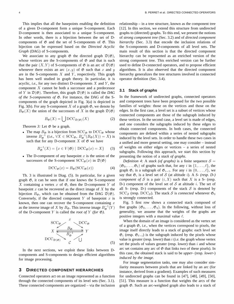
This implies that all the basepoints enabling the definitionof a given D-component form a unique S-component. EachD-component is then associated to a unique S-component.In other words, there is a bijection between the set of D-components ofG and the set of S-components ofG. Thisbijection can be expressed based on theDirected AcyclicGraph (DAG) of S-components.

We associate to any graphG the directed graphD(G),whose vertices are the S-components ofG and that is suchthat the pair(X,Y ) of S-components ofG is an arc ofD(G)whenever there exists an arc(x, y) of G such thatx and yare in the S-componentsX and Y , respectively. This graphhas been well studied in graph theory. In particular, it isacyclic, i.e., for any two distinct D-componentsX andY , thecomponentX cannot be both a successor and a predecessorof Y in D(G). Therefore, this graphD(G) is called theDAGof the S-components ofG. For instance, the DAG of the S-components of the graph depicted in Fig. 3(a) is depicted inFig. 3(b). For any S-componentX of a graphG, we denote byBG(X) the union of the successors ofX in the graphD(G)

BG(X) =⋃

DCCD(G)(X) (2)

Theorem 3:Let G be a graph.

• The mapBG is a bijection fromSCCG to DCCG whoseinverseB−1

G(i.e., ∀X ∈ SCCG, B−1

G(BG(X)) = X) is

such that for any D-componentX of G we have

B−1G

(X) = {x ∈ V (G) | DCCG(x) = X} (3)

• The D-component of any basepointx is the union of thesuccessors of the S-componentSCCG(x) in D(G)

DCCG(x) = BG(SCCG(x)) (4)

Th. 3 is illustrated in Diag. (5). In particular, for a givengraphG, it can be seen that if one knows the S-componentX containing a vertexx of G, then the D-componentY ofbasepointx can be recovered as the direct image ofX by thebijection BG, which can be obtained from the DAGD(G).Conversely, if the directed componentY of basepointx isknown, then one can recover the S-component containingxas the inverse image ofX by BG. This inverse imageB−1

G(Y )

of the D-componentY is called theroot of Y (for G).

x

C

X Y

................................................................................... ............

DCCG

................................................................................... ............

DCCD(G)

.......................................................................................................................................................................................................

.

............................................................................................................................................................................................

............

B−1G

.......................................................................................................................................................................................................

.

............................................................................................................................................................................................

............

BG

...............................................................................................

SCCG

...............................................................................................

⋃

(5)

In the next sections, we exploit these links between D-components and S-components to design efficient algorithmsfor image processing.

3 DIRECTED COMPONENT HIERARCHIES

Connected operators act on an image represented as a functionthrough the connected components of its level sets (Sec. 3.1).These connected components are organized – via the inclusion

relationship – in a tree structure, known as the component tree[12]. In this section, we extend this structure from undirectedgraphs to (directed) graphs. To this end, we present the notionsof strong component tree(Sec. 3.2) and ofdirected componenthierarchy (Sec. 3.3) that encode the inclusion relations ofthe S-components and D-components of all level sets. Themain result of this section is that the directed componenthierarchy can be represented as an enriched version of thestrong component tree. This enriched version can be furtherused to define D-connected operators, and to propose efficientalgorithms. It is also observed that the directed componenthierarchy generalizes the tree structures involved in connectedoperator definition (Sec. 3.4).

3.1 Stack of graphs

In the framework of undirected graphs, connected operatorsand component trees have been proposed for the two possiblefamilies of weights: those on the vertices and those on theedges. In the first case, a level set is a subset of vertices whoseconnected components are those of the subgraph induced bythese vertices. In the second case, a level set is made of edges,and one considers the subgraphs induced by these edges toobtain connected components. In both cases, the connectedcomponents are defined within a series of nested subgraphsinduced by the level sets. In order to handle these two cases ina unified and more general setting, one may consider – insteadof weights on either edges or vertices – a series of nestedsubgraphs. Following this approach, we start this section bypresenting the notion of astack of graphs.

Definition 4: A stack (of graphs)is a finite sequenceS =(G0, . . . ,Gℓ) of graphs such that, for anyi in {1, . . . , ℓ}, thegraphGi is a subgraph ofGi−1. For anyi in {0, . . . , ℓ}, wesay thatGi is a level set ofS (at altitudei). A S- (resp. D-)component ofS is a pair (i,X) such thatX is a S- (resp.D-) component of the level set ofS at altitudei. The set ofall S- (resp. D-) components of the stackS is denoted bySCCS (resp.DCCS ). The stackS is connectedwheneverG0

is strongly connected.Fig. 5 first row shows a connected stack composed of

five graphs(G0, . . . ,G4). In the following, without loss ofgenerality, we assume that the weights of the graphs arepositive integers with a maximal valueℓ.

When the domain of an image is considered as the vertex setof a graphG, i.e., when the vertices correspond to pixels, theimage itself directly leads to a stack of graphs: each level setGi (resp.Gℓ−i) is the subgraph induced by the pixels whosevalue is greater (resp. lower) thani (i.e. the graph whose vertexset the pixels of values greater (resp. lower) thani and whosearc set contains any arc ofG that links two of these pixels). Inthis case, the obtained stack is said to beupper-(resp.lower-)induced by the image.

For image segmentation tasks, one may also consider sim-ilarity measures between pixels that are linked by an arc (forinstance, derived from a gradient). Examples of such measuresfor undirected graphs can be found in [47], [48], [49], [50],[51]. This measure is a function that weights the arcs of thegraphG. Such an arc-weighted graph also leads to a stack of


Fig. 6. (a) The S-component tree associated to thestack S of Fig. 5, first row. (b) The DAGs shown fromtop to bottom row are the DAGs of S-components ofthe graphs G0, . . . ,G4 of Fig. 5, first row. (c) The D-component hierarchy of the stack S of Fig. 5, second row.This hierarchy is the S-component tree (a) enriched bythe relation provided by the DAGs of S-components of alllevel sets of S (b). The red arrows are the extra links thatare deduced by transitivity.

graphs: each level setGi (resp.Gℓ−i) is the subgraph inducedby the arcs of weight greater (resp. lower) thani (i.e., the graphwhose arc set contains any arc of weight greater (resp. lower)than i and whose vertex set contains any pixel ofG linkedby one of these arcs). Such a stack is said to beupper- (resp.lower-) induced by the similarity measure. For segmentationmethods based on hierarchies of partitions [13], [38], one maywant to ensure that all levels in the graph stack remain apartition of the domain by preserving all pixels as verticesofevery level set. This can ease further segmentation methodstoproduce partitions as shown in [18]. A stack obtained by thisprocess is said to becompleted.

Important notation. In the remaining part of this section,S = {G0, . . . ,Gℓ} denotes a connected stack.

3.2 Strong component tree

Let X be a S-component ofGi, for i in {1, . . . , ℓ}. SinceGi

is a subgraph ofGi−1, X is strongly connected inGi−1. Asthe S-components of a graph partition its vertex set, the S-componentX of Gi is included in a unique S-component ofGi−1. This unique S-component ofGi−1 that includesX isdenoted byPARi−1(X) and is called the(i− 1)-parent ofX(in S). We also say that the S-component(i−1,PARi−1(X))of S is the parent of the S-component(i,X). The set of allS-components ofS equipped with the parent relation is a treecalled thestrong component(or S-component) tree ofS.

Following the usual terminology on trees, given two S-components(i,X) and (j, Y ) of the stackS, we say that(j, Y ) is an ancestor of(i,X) and that(i,X) is a descen-dant of (j, Y ) if there exists a sequence(C0, . . . , Cn) of S-components ofS such thatC0 = (i,X), Cn = (j, Y ), andCk

is the parent ofCk−1 for any k ∈ {1, . . . , n}. For instance,Fig. 6(a) shows the S-component tree of the stack of Fig. 5.

3.3 Directed component hierarchy

Since distinct D-components of the same graph can be linkedby inclusion (see Sec. 2.2), it can be seen that for a given

i in {1, . . . , ℓ}, a D-component ofGi can be included inseveral D-components ofGi−1. Therefore, contrarily to thecase of S-components, the inclusion relations between D-components of successive level sets cannot be directly usedfororganizing the D-components in a tree structure. Fortunately,as we will see later in this section, the D-components can bearranged as a DAG that is sufficient to recover the inclusionrelationship between any two D-components. Furthermore, dueto the bijection between S-components and D-components (seeTh. 3), this DAG corresponds to an enriched version of theS-component tree. This structure leads to efficient methods,that are described in Secs. 4, 5, for designing D-connectedoperators. The next theorem is the key result for establishingthe properties of this fundamental DAG.

Theorem 5:Let X andY be two D-components ofGi andGi−1, respectively, withi in {1, . . . , ℓ}. The D-componentXis a subset of the D-componentY if and only if the (i − 1)-parent of the root ofX is a successor of the root ofY in theDAG of S-components ofGi

X ⊆ Y ⇐⇒ PARi−1(B−1Gi

(X)) ∈ DCCD(Gi−1)(B−1Gi−1

(Y ))(6)

More generally, a D-componentX of Gi is a subset of a D-componentY of Gj (with i ≥ j) if and only if the intersectionbetween the ancestors of the root ofX and the successors ofthe root of Y in D(Gj) is nonempty. In other words, theset of DAGs of the S-components of all level sets, paired tothe parent relation allows us to test the inclusion of any D-components belonging to the stackS.

Definition 6: The D-component hierarchy ofS is the graphwhose nodes are the S-components ofS and such that thereis an arc from a S-component(j, Y ) of S to a S-component(i,X) of S if

• (j, Y ) is the parent of(i,X); or• j = i and (Y,X) is an arc of the DAGD(Gi) of S-

components ofGi.For instance, the D-components of the stack in Fig. 5 are

depicted in the second row of Fig. 5. The associated D-component hierarchy is depicted in Fig. 6(c).

As a corollary to Th. 5, there is an isomorphism betweenthe order induced by the D-component hierarchy of the stackS and the partial order on the D-components ofS such that(i,X) ⊑ (j, Y ) if i ≤ j and X ⊆ Y . In particular, the S-component(j, Y ) is the parent of(i,X) if and only ifBGj

(Y )is the minimal element (for the inclusion relation) amongall the D-components ofGj that include the D-componentBGi

(X). A direct consequence of this isomorphism is thatthe D-component hierarchy ofS is a DAG. In particular, twoS-components at the same level set cannot be linked by a cyclesince the DAG of S-components of a graph is acyclic. It canalso be seen that two S-components of two distinct level setscannot be linked by a cycle either since a S-component of agiven level set cannot be both an ancestor and a descendantof a S-component of another level set.

3.4 Generalization of tree structures

The framework presented in this section for handling thecomponents of a stack of graphs generalizes the handling of


(f) G0 (g) G1 (h) G2 (i) G3 (j) G4

Fig. 5. A stack S = (G0,G1,G2,G3,G4). First row: Each color represents a S-component. Second row: Each colorrepresents a D-component (vertices with more than one color belong to all the associated D-components).

connected components via component trees, in both edge- andvertex-weighted undirected graphs.

Indeed, it can be seen that if a graph is symmetric, then a setof vertices is a D-component if and only if it is a connectedcomponent in the associated undirected graph. Furthermore,such a set is a D-component if and only if it is a S-component.Hence, in the case of a stack whose level sets are all symmetricgraphs, the D-component hierarchy and the S-component treeare indeed the same. Moreover, if a stack is upper (resp. lower)induced by an image, then its D-component hierarchy is alsothe max- (resp. min-) tree of that image. If a stack is upper(resp. lower) induced by an arc similarity measure, then itsD-component hierarchy is the max- (resp. min-) tree of theassociated undirected edge-weighted graph. In this last case,if the stack is furthermore completed, then the D-componenttree is exactly the partition tree [18] (also known as thequasi flat zones hierarchy [38], [52], [53] orα-tree [54]) ofthe image. As shown in [18], completed stacks also allowus to retrieve the binary partition trees [13] and hierarchicalminimum spanning forests or watersheds [55] [11, Ch. 9] [56].

4 BUILDING D-COMPONENT HIERARCHIES

In this section, we describe how to build the D-component hi-erarchy of a stack of graphsS = {G0, . . . ,Gℓ} (Sec. 4.1), andwe discuss the computational cost of this process (Sec. 4.2).

4.1 Algorithm

For the sake of concision, we assume here that the stackS is constructed from a vertex-weighted graphG = (V,A)(see Sec. 3.1). We also assume that graphs are represented byadjacency lists: for each vertexx of V , we store the list ofverticesy of V adjacent tox (i.e., such that(x, y) is in A).This representation allows us to access to the list of verticesadjacent to a given vertex in constant time.

The overall construction procedure is described in Alg. 1.Its results consist of: a labeling of each level of the stackSinto S-components (Labeli), the adjacency lists of the DAGs

of S-components at each level of the stack (Suci), and theparent relation between the S-components of successive levelsof the stack (PARi).

For each leveli of the stack, the algorithm consists ofthree steps: (1) label the vertices ofGi into S-components; (2)construct the DAG of S-components ofGi, i.e., the adjacencylists representing the DAG; and (3) define the parent relationbetween these S-components and those at altitudei+ 1.

Step (1) is carried out by either the Tarjan [57] or Kosaraju-Sharir [58] algorithms, which both produce a labeling inS-components of the vertices of a directed graph in linearO(|V | + |A|) time. We assume that the labels are integersand that the labels at the different levels are all distinct (i.e.,Labeli ∩ Labelj = ∅ for i 6= j); so they can be used as arrayindices. For the sake of readability, we consider that the resultLabeli is at the same time the set of labels ofD(Gi), denotedby Labeli, and the map that associates a label, denoted byLabeli[x], to each vertexx of V (Gi).

Step (2) is performed by Alg. 2. It produces the adjacencylist of each vertex of the DAG of the S-components of the levelset ofG at altitudei. To this end, it successively scans eachS-component ofGi. For any scanned S-componentSCC[v]of label v, the adjacent vertices of all the vertices inSCC[v]are considered. If one of these adjacent vertices belongs toanother S-componentSCC[v′] of label v′ (i.e., if v′ 6= v, line11), and if SCC[v′] has not yet been reached fromSCC[v](i.e., if Flag[v′] 6= v, line 11), then the labelv′ is added tothe adjacency list ofv (line 12), andv′ is flagged as havingbeen reached fromv (line 13). The two outer loops visit eachvertex once, and for each vertex, its adjacency list is scanned.The algorithm can thus be run in linearO(|V |+ |A|) time.

Step (3) is performed by Alg. 3 which produces an arraysuch that, for every labelv of the S-component labeling atlevel i+ 1, the element of indexv in the array is the label ofthe S-component in the leveli that includes the S-componentv. The algorithm loops through each vertexx in V (Gi+1)of the previous leveli + 1, and finds the labelsLabeli+1[x]and Labeli[x] of its associated S-components at levelsi + 1


Algorithm 1: D-component hierarchy construction.Input: S = {G0, . . . ,Gℓ}, a stack of graphs.Output: Labeli, S-component labeling for eachi in {0, . . . , ℓ}.Output: Suci, array of adjacency lists for eachi in {0, . . . , ℓ}.Output: PARi, parent relation for eachi in {0, . . . , ℓ}.

1 for i from ℓ to 0 do2 Labeli ← S-component labeling(Gi)3 Suci ← adjacency lists(Gi, Labeli)4 if i 6= ℓ then5 PARi+1 ← parent relation(Gi+1, Labeli+1, Labeli)

Algorithm 2: Adjacency lists construction.Input: Gi, a graph.Input: Labeli, S-component labeling ofGi.Output: Suci, array of adjacency lists ofGi.

1 foreach v ∈ Labeli do2 Suci[v]← ∅3 SCC[v]← ∅4 Flag[v]← undefined

5 foreach x ∈ V (Gi) do6 SCC[Labeli[x]]← SCC[Labeli[x]] ∪ {x}

7 foreach v ∈ Labeli do8 foreach x ∈ SCC[v] do9 foreach (x, y) ∈ A(Gi) do

10 v′ ← Labeli[y]11 if v′ 6= v and Flag[v′] 6= v then12 Suci[v]← Suci[v] ∪ {Labeli[y]}13 Flag[y]← v

Algorithm 3: Parent relation definition.Input: Gi+1, a directed graph.Input: Labeli+1, a labeling of the S-components ofGi+1.Input: Labeli, a labeling of the S-components ofGi.Output: PARi+1, parent relation onLabeli+1 andLabeli.

1 foreach x ∈ V (Gi+1) do2 PAR[Labeli+1[x]]← Labeli[x]

and i. It then defines the labelLabeli[x] as the parent ofthe label Labeli+1[x]. In order to achieve a linearO(|V |)complexity, the labels have to be determined in constant timewhich is achieved by storing them for each vertex during theS-component labeling.

4.2 Complexity analysis

The time complexity of Alg. 1 isO(ℓ.(|V |+|A|)). In particularthe algorithm is efficient ifℓ is small, for instance in the caseof 8-bit images. As there are at most|V | levels (each vertexcan have a different weight), this complexity is bounded byO(|V |(|V | + |A|)). However, if we do not restrict ourselvesto vertex-weighted graphs, there are at most|V |+ |A| levels(each vertex and arc is added one after the other), so in theworst case, this leads to a complexity ofO((|V | + |A|)2).However, one can generally assume thatℓ ≪ |V |+ |A|.

The algorithm can be improved by observing that a S-component at leveli is strongly connected at leveli−1. Thus,we can use a more complex algorithm to build the subgraph

at level i. Instead of considering the graph induced by thevertices of weights higher thani, we can add to the DAGof S-components at leveli− 1, the vertices and the arcs thatappear at leveli. This requires the use of a union-find structureto dynamically manage the S-components. This generates anadditional cost leading to aO(α(|V |).(|V |+ |A|)2) worst casecomplexity, whereα is the extremely slowly growing inverseof the Ackermann function. Practically, we have verified thatthe improved algorithm is about six times faster than the basicone.

5 SELECTING NODES

Similarly to connected operators, D-connected operators con-sist of processing a hierarchical data structure, namely theD-component hierarchy. This processing requires selecting ordiscarding nodes according to criteria that are specificallydefined according to the considered application (Sec. 5.1).Theselected nodes can then be used,e.g., to obtain a segmentationor to filter an image. Some applications will be described inSec. 6. Since D-component hierarchies are not tree structures,D-connected operators are more difficult to develop thanclassically connected ones (Sec. 5.2). In particular, theyrequirespecific regularization strategies (Sec. 5.3).

5.1 Node selection criteria

A node selection criterionσ is a predicate associating aBoolean value to each node/component of a hierarchical datastructure. Given a componentC, we say that the criterionσholds true(resp.false) for C, or thatC satisfies(resp.violates)σ if σ(C) equals true (resp. false).

A classical criterionσA that discards small nodes, oftenassociated to noise, is defined by

σA(C) =

{

true if Area(C) > tfalse otherwise

(7)

where Area is a measure of the area of the component, forexample the number of vertices inC, while t is the areathreshold value.

Many other criteria have been proposed in the literature.Most are obtained by replacing Area by some other attributein Eq. (7). Proposed attributes focus on different aspects:(1)the shape of the component,e.g., the geometrical moments orthe compactness; (2) the gray level content of the component,e.g., the volume or the entropy; (3) the topology of thehierarchy,e.g., the number of children of the component; or(4) combination of the previous types of attributes,e.g., thedynamic or the Mumford-Shah energy. It is also possible toreplace a constant threshold by a more complex process inthe definition of the criterion,e.g., criteria based on energyminimization (Viterbi in [12]) or on shape-space filtering [42].

5.2 The case of D-connected operators

Thinking in terms of D-connected operators, one may desireto mark each D-component as selected or discarded. However– in contrast to the case of connected operators – we may fallinto situations such as the one depicted in Fig. 4(b), where two


A B C

(a) Hi

A B C

(b) Hi

A B C

(c) Hi

B C

(d) σ1

A B

(e) σ2

A C

(f) σ3

A

(g) σ1

C

(h) σ2

B

(i) σ3

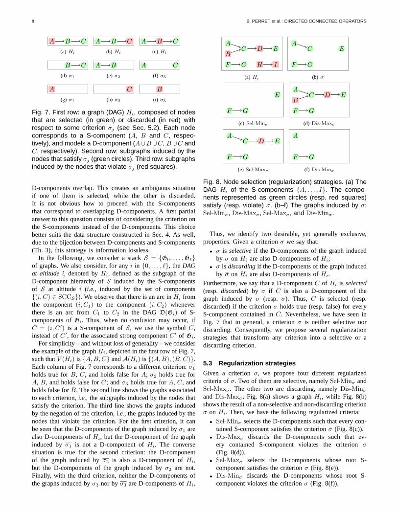
Fig. 7. First row: a graph (DAG) Hi, composed of nodesthat are selected (in green) or discarded (in red) withrespect to some criterion σj (see Sec. 5.2). Each nodecorresponds to a S-component (A, B and C, respec-tively), and models a D-component (A∪B∪C, B∪C andC, respectively). Second row: subgraphs induced by thenodes that satisfy σj (green circles). Third row: subgraphsinduced by the nodes that violate σj (red squares).

D-components overlap. This creates an ambiguous situationif one of them is selected, while the other is discarded.It is not obvious how to proceed with the S-componentsthat correspond to overlapping D-components. A first partialanswer to this question consists of considering the criterion onthe S-components instead of the D-components. This choicebetter suits the data structure constructed in Sec. 4. As well,due to the bijection between D-components and S-components(Th. 3), this strategy is information lossless.

In the following, we consider a stackS = {G0, . . . ,Gℓ}of graphs. We also consider, for anyi in {0, . . . , ℓ}, theDAGat altitude i, denoted byHi, defined as the subgraph of theD-component hierarchy ofS induced by the S-componentsof S at altitude i (i.e., induced by the set of components{(i, C) ∈ SCCS}). We observe that there is an arc inHi fromthe component(i, C1) to the component(i, C2) wheneverthere is an arc fromC1 to C2 in the DAG D(Gi) of S-components ofGi. Thus, when no confusion may occur, ifC = (i, C ′) is a S-component ofS, we use the symbolC,instead ofC ′, for the associated strong componentC ′ of Gi.

For simplicity – and without loss of generality – we considerthe example of the graphHi, depicted in the first row of Fig. 7,such thatV (Hi) is {A,B,C} andA(Hi) is {(A,B), (B,C)}.Each column of Fig. 7 corresponds to a different criterion:σ1

holds true forB, C, and holds false forA; σ2 holds true forA, B, and holds false forC; andσ3 holds true forA, C, andholds false forB. The second line shows the graphs associatedto each criterion,i.e., the subgraphs induced by the nodes thatsatisfy the criterion. The third line shows the graphs inducedby the negation of the criterion,i.e., the graphs induced by thenodes that violate the criterion. For the first criterion, itcanbe seen that the D-components of the graph induced byσ1 arealso D-components ofHi, but the D-component of the graphinduced byσ1 is not a D-component ofHi. The conversesituation is true for the second criterion: the D-componentof the graph induced byσ2 is also a D-component ofHi,but the D-components of the graph induced byσ2 are not.Finally, with the third criterion, neither the D-components ofthe graphs induced byσ3 nor byσ3 are D-components ofHi.

AC E

F G

BD

H I

(a) Hi

AC E

F G

(b) σ

E

F G

(c) Sel-Minσ

AC E

F G

BD

(d) Dis-Maxσ

AC E

F G

D

(e) Sel-Maxσ

A

F G

(f) Dis-Minσ

Fig. 8. Node selection (regularization) strategies. (a) TheDAG Hi of the S-components {A, . . . , I}. The compo-nents represented as green circles (resp. red squares)satisfy (resp. violate) σ. (b–f) The graphs induced by σ:Sel-Minσ, Dis-Maxσ, Sel-Maxσ, and Dis-Minσ.

Thus, we identify two desirable, yet generally exclusive,properties. Given a criterionσ we say that:

• σ is selectiveif the D-components of the graph inducedby σ on Hi are also D-components ofHi;

• σ is discardingif the D-components of the graph inducedby σ on Hi are also D-components ofHi.

Furthermore, we say that a D-componentC of Hi is selected(resp. discarded) by σ if C is also a D-component of thegraph induced byσ (resp. σ). Thus, C is selected (resp.discarded) if the criterionσ holds true (resp. false) for everyS-component contained inC. Nevertheless, we have seen inFig. 7 that in general, a criterionσ is neither selective nordiscarding. Consequently, we propose several regularizationstrategies that transform any criterion into a selective oradiscarding criterion.

5.3 Regularization strategies

Given a criterionσ, we propose four different regularizedcriteria ofσ. Two of them are selective, namelySel-Minσ andSel-Maxσ. The other two are discarding, namelyDis-MinσandDis-Maxσ. Fig. 8(a) shows a graphHi, while Fig. 8(b)shows the result of a non-selective and non-discarding criterionσ on Hi. Then, we have the following regularized criteria:

• Sel-Minσ selects the D-components such that every con-tained S-component satisfies the criterionσ (Fig. 8(c)).

• Dis-Maxσ discards the D-components such that ev-ery contained S-component violates the criterionσ(Fig. 8(d)).

• Sel-Maxσ selects the D-components whose root S-component satisfies the criterionσ (Fig. 8(e)).

• Dis-Minσ discards the D-components whose root S-component violates the criterionσ (Fig. 8(f)).


Thus, for any leveli of the hierarchy and for any componentC of the DAGHi at altitudei, we have

Sel-Minσ(C) =∧

C′∈DCCHi(C)

σ(C ′) (8)

Dis-Maxσ(C) =∨

C′∈DCCHi(C)

σ(C ′) (9)

Sel-Maxσ(C) =∨

C∈DCCHi(C′)

σ(C ′) (10)

Dis-Minσ(C) =∧

C∈DCCHi(C′)

σ(C ′) (11)

where∧

and∨

are the Boolean “and” and “or” operators.Property 7: Let σ be a criterion on the D-component

hierarchy of the stackS = {G0, . . . ,Gℓ}. The regularizedcriterion Sel-Maxσ (resp.Dis-Minσ) with respect toS is thesame as the regularized criterionDis-Maxσ (resp.Sel-Minσ)with respect to the transpose stack−S = {−G0, . . . ,−Gℓ},where−Gi is the transpose of the graphGi. More precisely,for any DAGHi at altitudei of S and for any componentCof Hi, we have:

∨

C∈DCCHi(C′)

σ(C ′) =∨

C′∈DCC−Hi(C)

σ(C ′) (12)

∧

C∈DCCHi(C′)

σ(C ′) =∧

C′∈DCC−Hi(C)

σ(C ′) (13)

Remark 8:The simplest criteria – that include in particularthe criterionσA – are those that areincreasing. We say thata criterion σ is increasing if, for any two S-componentsCand C ′ such that the D-component rooted inC is includedin the D-component rooted inC ′, σ(C) = true implies thatσ(C ′) = true. So, given an increasing criterionσ and a S-componentC, if σ holds true forC, we immediately know thatall the predecessors ofC also satisfyσ. Conversely, ifσ holdsfalse forC, we immediately know that all the successors ofCviolate σ, or, in other words, all the S-components containedin the D-component of rootC violate the criterion. Thus, anyincreasing criterionσ is discarding. In this case,σ is equal toDis-Minσ and toDis-Maxσ.

The previous discussions focused on node selection for asingle level of the hierarchy. Nevertheless, a similar challengeexists in order to ensure result consistency between the dif-ferent levels of the hierarchy,i.e., in order to avoid “holes”between two or more levels.

The previously defined regularization rules can also be usedon the S-component tree, by considering the ancestors (resp.descendants) instead of the the predecessors (resp. successors)These new – but similar – hierarchical criteria are denotedSel-Max-H, Sel-Min-H, Dis-Max-H, andDis-Min-H:

• Sel-Max-Hσ holds true for all the descendants of a nodethat satisfiesσ.

• Sel-Min-Hσ holds false for all the ancestors of a nodethat violatesσ.

• Dis-Min-Hσ holds false for the descendants of a nodethat violatesσ.

• Dis-Max-Hσ holds true for all the ancestors of a nodethat satisfiesσ.

In effect, theDis-Min-Hσ (resp.Dis-Max-Hσ) strategy is theanalogue of the usual min (resp. max) filtering rules of theclassical component trees [12].

Remark 9:Increasing criteria are consistent with the parent-child relation. Given a criterionσ and two S-componentsCandC ′ such thatC ′ is a descendant ofC (i.e., C ′ ⊆ C), theD-component rooted inC ′ is included in the D-componentrooted inC, and thusσ is increasing ifσ(C ′) = true impliesσ(C) = true (which is the usual definition of an increasingcriterion). Thus, for an increasing criterionσ, all the proposedregularization strategies ofσ yield the same result asσ due tothe tree structure of the S-components at the different levels(by opposition to the DAG of the S-components at a singlelevel).

6 EXPERIMENTS AND DISCUSSION

In this section we illustrate the relevance of the proposedD-component hierarchy framework. This relevance derivesfrom its compliance with efficient image processing paradigmsalready proposed in the literature. This is notably the caseof the non-local approaches, as discussed in Sec. 6.1, andshown by an experimental validation in the context of retinalimage analysis. The versatility of the D-component hierarchyframework is exemplified by proposing two applications inSec. 6.2: one in neurite image filtering and the other in cardiacimage segmentation.

6.1 D-component hierarchy and non-locality

Local approaches for image processing rely on the assumptionthat neighboring pixels are often strongly correlated. In thegraph-based formalism, this is generally interpreted by con-sidering standard – symmetric – adjacency relations onZ

2 orZ3, that model such spatial neighborhoods [59].In contrast, non-local approaches consider correspondence

between pixels that are closely related from a statistical –instead of spatial – point of view. In this framework, allpixels are adjacent to one another. Each adjacency link isweighted by a distance that models the similarity betweenpixels, or more typically between regions around them (apatch). This approach was popularized in [60] and [44] forimage segmentation and filtering and extended to segmenta-tion, reconstruction [61] and classification [62].

A common issue with this approach is its algorithmiccomplexity. In the graph-based formalism, non-locality impliesmapping a complete graph onto the processed image, leadingto prohibitive computational costs. Practically, the non-localapproach is approximated in a fashion similar tok-nearestneighbors, bya priori limiting potential pairing betweenpixels, for instance based on spatial distance. In so doing,the graph modeling the image becomes sparse, and it alsobecomes directed. Indeed, a pixelb can be within thek-nearestneighbors of a pixela while a is not within those ofb, forinstance due to window size restrictions [44]. In particular,involving non-local approaches in hierarchical frameworksnaturally leads to handling D-component hierarchies.

In previous works, these asymmetric, directed adjacenciesare not fully exploited, for instance in [60] where the graph


(a) Image 2 of DRIVE (b) Filter IHσRV(c) Segmentation

(d) Image 19 of DRIVE (e) Filter IHσRV(f) Segmentation

Fig. 9. Segmentation results on the DRIVE database. Oneach row, from left to right: pre-processed image, filteringresult, and evaluation of the segmentation.

is symmetrized. We propose to use this directed informationin the D-component framework to achieve improved results.

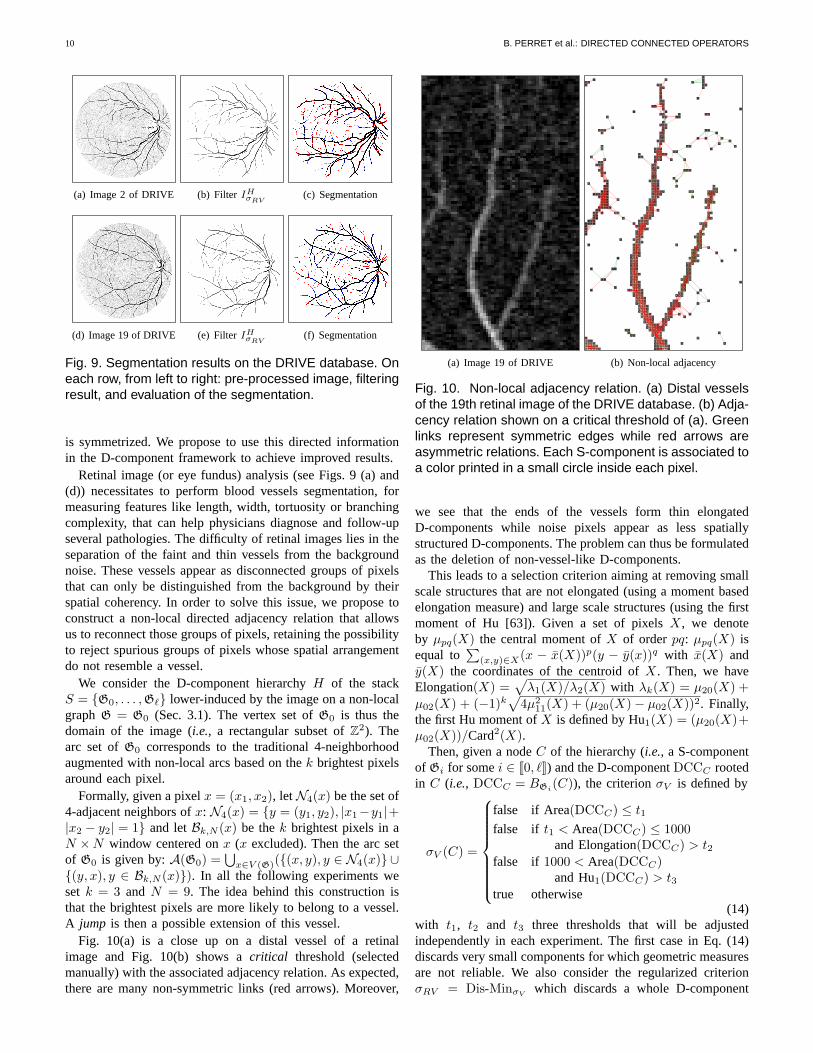
Retinal image (or eye fundus) analysis (see Figs. 9 (a) and(d)) necessitates to perform blood vessels segmentation, formeasuring features like length, width, tortuosity or branchingcomplexity, that can help physicians diagnose and follow-upseveral pathologies. The difficulty of retinal images lies in theseparation of the faint and thin vessels from the backgroundnoise. These vessels appear as disconnected groups of pixelsthat can only be distinguished from the background by theirspatial coherency. In order to solve this issue, we propose toconstruct a non-local directed adjacency relation that allowsus to reconnect those groups of pixels, retaining the possibilityto reject spurious groups of pixels whose spatial arrangementdo not resemble a vessel.

We consider the D-component hierarchyH of the stackS = {G0, . . . ,Gℓ} lower-induced by the image on a non-localgraphG = G0 (Sec. 3.1). The vertex set ofG0 is thus thedomain of the image (i.e., a rectangular subset ofZ2). Thearc set ofG0 corresponds to the traditional 4-neighborhoodaugmented with non-local arcs based on thek brightest pixelsaround each pixel.

Formally, given a pixelx = (x1, x2), letN4(x) be the set of4-adjacent neighbors ofx: N4(x) = {y = (y1, y2), |x1−y1|+|x2 − y2| = 1} and letBk,N (x) be thek brightest pixels in aN ×N window centered onx (x excluded). Then the arc setof G0 is given by:A(G0) =

⋃

x∈V (G)({(x, y), y ∈ N4(x)} ∪{(y, x), y ∈ Bk,N (x)}). In all the following experiments weset k = 3 andN = 9. The idea behind this construction isthat the brightest pixels are more likely to belong to a vessel.A jump is then a possible extension of this vessel.

Fig. 10(a) is a close up on a distal vessel of a retinalimage and Fig. 10(b) shows acritical threshold (selectedmanually) with the associated adjacency relation. As expected,there are many non-symmetric links (red arrows). Moreover,

(a) Image 19 of DRIVE (b) Non-local adjacency

Fig. 10. Non-local adjacency relation. (a) Distal vesselsof the 19th retinal image of the DRIVE database. (b) Adja-cency relation shown on a critical threshold of (a). Greenlinks represent symmetric edges while red arrows areasymmetric relations. Each S-component is associated toa color printed in a small circle inside each pixel.

we see that the ends of the vessels form thin elongatedD-components while noise pixels appear as less spatiallystructured D-components. The problem can thus be formulatedas the deletion of non-vessel-like D-components.

This leads to a selection criterion aiming at removing smallscale structures that are not elongated (using a moment basedelongation measure) and large scale structures (using the firstmoment of Hu [63]). Given a set of pixelsX, we denoteby µpq(X) the central moment ofX of orderpq: µpq(X) isequal to

∑

(x,y)∈X(x − x(X))p(y − y(x))q with x(X) andy(X) the coordinates of the centroid ofX. Then, we haveElongation(X) =

√

λ1(X)/λ2(X) with λk(X) = µ20(X) +

µ02(X) + (−1)k√

4µ211(X) + (µ20(X)− µ02(X))2. Finally,

the first Hu moment ofX is defined by Hu1(X) = (µ20(X)+µ02(X))/Card2(X).

Then, given a nodeC of the hierarchy (i.e., a S-componentof Gi for somei ∈ [[0, ℓ]]) and the D-componentDCCC rootedin C (i.e., DCCC = BGi

(C)), the criterionσV is defined by

σV (C) =

false if Area(DCCC) ≤ t1

false if t1 < Area(DCCC) ≤ 1000and Elongation(DCCC) > t2

false if 1000 < Area(DCCC)and Hu1(DCCC) > t3

true otherwise(14)

with t1, t2 and t3 three thresholds that will be adjustedindependently in each experiment. The first case in Eq. (14)discards very small components for which geometric measuresare not reliable. We also consider the regularized criterionσRV = Dis-MinσV

which discards a whole D-component


whenever its root S-component does not satisfyσV .The D-component hierarchy can be used to perform image

filtering, i.e., to obtain a new image based on the nodeselection procedure. This requires to define thereconstructionIHσ of the hierarchyH with respect to the criterionσ as afunction that maps each vertexv of G0 to the altitude of thesmallest node ofH that satisfiesσ and that containsv

IHσ (v) =max{i ∈ [[0, ℓ]] |

(i, C) ∈ V (H), v ∈ C, σ((i, C)) = true} (15)

Figs. 9 (b) and (e) show the results of retinal image filteringusing the criterionσRV . The resulting filtered image is quiteclean. A final segmentation is obtained by selecting every non-zero pixel from this filtered image.

The following results rely on the DRIVE (Digital Reti-nal Images for Vessel Extraction) database [64], which iscomposed of 20 test images. Each image of size 565×584pixels is encoded in 24 bits RGB and comes with 2 expertsegmentations and a mask of the eye fundus. The segmentationof an image is evaluated with 3 measures (pixels outside theeye fundus mask do not count): the true positive rate (TPR)(resp. true negative rate (TNR)) is the number of true positive(resp. negative) pixels divided by the total number of positive(resp. negative) pixels, and the accuracy is the sum of truepositive and negative pixels divided by the total number ofpixels. The score on the base is the mean of the image scoresplus the standard deviation of the accuracy (that measures thestability of the algorithm). In our experiments, we used onlythe green channel, which is pre-processed using a black top-hat (difference between a closing and the original image) witha disk structuring element of diameter 5 pixels. This operationflattens the background of the image and inverts its contrast.

Method TPR TNR Accuracy (σ)2nd expert 0.7761 0.9725 0.9473 (0.0048)RNL D-components (15,0.2,1) 0.7079 0.9790 0.9442 (0.0063)NL D-components (15,0.2,1) 0.7046 0.9790 0.9439 (0.0064)NL S-components (30,0.15,1.3) 0.7024 0.9789 0.9434 (0.0070)NL symmetric (Max) (15,0.2,1.3) 0.6528 0.9828 0.9404 (0.0083)NL symmetric (Min) (15,0.15,1.35) 0.6980 0.9786 0.9425 (0.0067)Xu [65] (local symmetric) 0.6924 0.9779 0.9413 (0.0078)Mendonça [66] 0.7344 0.9764 0.9452 (0.0062)Staal [64] 0.7193 0.9773 0.9442 (0.0065)

TABLE 1Result comparison on the DRIVE retinal image database.The methods of the first group are all connected filters.

The last two methods are the state of the art.

We have conducted a set of experiments (see Tab. 1) in orderto clearly identify the benefit of each aspect of the method.The evaluated methods are (the best found parameter values(t1, t2, t3) for the criteriaσV and σRV are given in Tab. 1after the method name):

1) RNL D-components: regularized criterionσRV on thenon-local asymmetric adjacency;

2) NL D-components: criterionσV on the non-local asym-metric adjacency;

3) NL S-components: same as above but where the criterionσV computes the features (area, elongation, Hu1) on theS-components instead of the D-components;

4) NL symmetric (Max): criterion σV on a non-local sym-metric adjacency where the edge(p, q) belongs to theadjacency if the edges(q, p) or (p, q) are in the asym-metric adjacency;

5) NL symmetric (Min): criterion σV on a non-local sym-metric adjacency where the edge(p, q) belongs to theadjacency if (p, q) and (q, p) are in the asymmetricadjacency;

6) Xu: connected attribute filter proposed in [65] on a localand symmetric graph with a complex morphologicalfiltering strategy;

Mendonça [66] and Staal [64] provide the state of the artmethods. It can be noted that, with Mendonça, the parametersof the method are adjusted independently for each image, theirmethodology differs thus from the classical one.

The results show that the proposed method 1) achievesthe same performances as Stall. In 2) when one removes theregularization strategy, the accuracy goes a bit down showingthat the notion of D-component is indeed a good model forvessels in this application. In 3) all the information aboutD-components is dropped: thus, the method relies only on theS-component tree. The accuracy is lower than in 1) and 2)which shows the interest of exploiting the adjacency relationamong the S-components (i.e., the DAG of S-components). In4) and 5) we measure the gain due to the asymmetric approach.For this, we construct two symmetric non-local adjacencyfollowing two classical strategies: min (only symmetric edgesare kept) and max (every edge is symmetrized). In both casesthe score is lower than in every other experiment. Whilethe max strategy leads to connecting a lot of noise to thevessels (with no mean to disconnect it), the min strategyis indeed quite close to a local approach as most non-localedges of the asymmetric adjacency are asymmetric. 6) is aconnected attribute filters (local symmetric adjacency) witha complex node selection strategy recently proposed in [65]which provides a reference score for classical connected filters.

All these experiments show the importance of each elementof the method – non-locality (1, 2, 3, 4, and 5), asymmetry andS-components (1, 2, and 3), D-component (1 and 2), regular-ization (1) – with a gradual improvement of the performanceswhen they are combined.

6.2 Other application examples

6.2.1 Neurite filteringThe proposed framework was also used to filter a sampleimage of a neuron with associated neurites (i.e., its axonand dendrites), grown in vitro (Fig. 1(a)). We rely on avesselness-like local object characterization [43], which en-ables us to classify pixels into tubes, blobs and background.We constructed an undirected pixel adjacency graph where apixel classified as a tube is linked to its 4-adjacent neighborsclassified as blobs but not the other way around. However,two 4-adjacent pixels of the same class are linked in bothdirections, while any background pixel is linked to all its 4-adjacent pixels. The vertices of this directed graph are thenweighted by the gray values of the corresponding pixels andthe associated D-component hierarchy is built. Relevant nodes


of the hierarchy are selected by a criterion using two heuristics:(1) a tube must have a (directed) connection with at least twoother structures; and (2) a tube is connected at its extremities:the length of the interval between a tube and the structuresit is connected to should be small. Similar criteria cannot bedesigned in the framework of component tree on undirectedgraphs, since in that framework a component cannot be con-nected to another (otherwise the two connected componentswould not be maximal connected sets). Then, from the selectedcomponents, a filtered image can be reconstructed (Fig. 1(b)).More details on this illustration are provided in an appendixsection, which can be found on-line as supplemental material.

6.2.2 Marker based segmentation

In this section, a D-component hierarchy is used in a markerbased image segmentation procedure. To this end, we builda directed arc-weighted graph from the image which is tobe segmented. Intuitively, this weighted graph correspondsto a directed gradient. Then, we construct the D-componenthierarchy associated to this graph and select D-componentsinorder to obtain a segmentation. The D-components are selectedusing user-provided markers of the object of interest and ofthe background. More precisely, a D-component is selectedwhenever it is rooted in a pixel marked as object and it doesnot contain any pixel marked as background. The resultingsegmentation is the union of the selected D-components.

Fig. 11 illustrates this procedure for the segmentation ofthe myocardium in a MRI of the heart. A weighted directed4-adjacency graph is obtained from a rough pre-classificationof the image pixels that produces a lot of false negativebackground pixels but tends to minimize the false positive (seeFig. 11(c)). This classification is obtained by excluding theextremal intensity values, which corresponds to blood and fatfor the brightest pixels and to lungs for the darkest. Then, theweight of an arc(x, y) between two 4-adjacent pixelsx andyis obtained as the absolute difference of intensity betweenxandy if y is not “pre-classified as background” or it is set toKtimes the absolute difference of intensity betweenx and yif y is pre-classified as background. Figs. 11(d) and (f) showthe results obtained whenK = 1 and K = 1.5. Note thatwhenK = 1 the weights of an arc(x, y) and of its symmetric(y, x) are always the same and correspond to the magnitudeof a simple intensity gradient. In this case, our method isthe same as [13], [67] for undirected graphs with symmetricedge-weights. However, whenK is greater than 1, the arcweights are not symmetric and the proposed weighting strategytends to facilitate the connection of the pixels pre-classified asbackground to the background marker. Fig. 11 clearly showsthis behavior and therefore illustrate the benefits of the directednon-symmetric method over its undirected symmetric variant.More details on this method, including a link with the notionofconnection value [68], [69] and the oriented IFT segmentationframework [5] can be found on-line as supplemental material.

7 CONCLUSION

We have introduced and investigated a notion of directed con-nectedness. This has led us to the proposal of new (directed)

connected operators, no longer based on partition hierarchiesorganized as trees, but on partition covers organized as DAGs.

From a theoretical viewpoint, we have provided a relevantway to generalize various tree-based connected operatorspreviously proposed in the literature. This may lead to abetter understanding of the common properties between theseoperators, and also helps to clarify some subtle differencesbetween those that lie in the framework of directed connectedoperators, and those that do not, such as hyperconnections.In this context, it is relevant to develop an axiomatizationofdirected connectedness such as was done in [70], in orderto compare it to the axiomatizations already proposed forconnections [45, Ch. 2] and hyperconnections [71].

From both the theoretical and algorithmic viewpoints, it mayalso be useful to compare the links that exist between theDAGs induced by directed connectedness, with other non-treestructures that have been recently introduced to extend theframework of connected operators, for instance in the case ofhypertrees [37] or component graphs [72], [73], that constitutean extension of component trees to multivalued images.

From a methodological viewpoint, we have shown that thecover hierarchies obtained when considering directed con-nectedness can be efficiently handled by taking advantageof the intrinsic links that exist between directed connectedand strongly connected components, the latter being organizedin trees. Based on these properties, the complexity of theinitial algorithm proposed in this article for building coverhierarchies, can be improved by using the recent incrementalalgorithm proposed in [74] for building the DAG of stronglyconnected components inO(N3/2) time complexity. More-over, beyond the standard attribute-based anti-extensivefiltersdeveloped in this article, other approaches initially devoted totree structures can be adapted to the case of directed connectedoperators, and in particular the optimal tree-cut segmentationparadigms initially proposed in [40], and further formalized inthe framework of connected operators [75].

From the applicative viewpoints, we have shown that thedirected connectedness framework is suitable for efficientlyhandling non-local image processing paradigms, in their –standard –k nearest neighbor version. The directed connect-edness framework is also quite versatile and then useful forvarious filtering and segmentation tasks. Applications will bemore extensively proposed in further works, in particular bycomparisons with similar approaches proposed in the litera-ture, for instance in [5].

Source code corresponding to this article is available at thefollowing url: http://www.esiee.fr/~perretb/dc-hierarchy.html.

ACKNOWLEDGMENT

This work was funded with FrenchAgence Nationale de laRecherchegrant agreements ANR-10-BLAN-0205 and ANR-12-MONU-0010.

REFERENCES

[1] A. Rosenfeld, “Connectivity in digital pictures,”J Assoc Comput Mach,vol. 17, pp. 146–160, 1970.

[2] ——, “Adjacency in digital pictures,”Inform Control, vol. 26, pp. 24–33,1974.

http://www.esiee.fr/~perretb/dc-hierarchy.html


(a) Original (b) O: myocardium (c) B: background (d) Symmetric result (e) S0: Over-segm. (f) Directed result

Fig. 11. Segmentation based on the D-component hierarchy. (b,c,e) The considered sets are superimposed in red tothe original image. (d,f) The internal border of the segmentation results are superimposed in red to the original image.

[3] Y. Boykov and G. Funka-Lea, “Graph cuts and efficient N-D imagesegmentation,”Int J Comput Vision, vol. 70, pp. 109–131, 2006.

[4] D. Singaraju, L. Grady, and R. Vidal, “Interactive image segmentationvia minimization of quadratic energies on directed graphs,” in CVPR,2008.

[5] P. A. V. Miranda and L. A. C. Mansilla, “Oriented image forestingtransform segmentation by seed competition,”IEEE T Image Process,vol. 23, pp. 389–398, 2014.

[6] O. Tankyevych, H. Talbot, and N. Passat, “Semi-connections and hier-archies,” inISMM, 2013, pp. 157–168.

[7] H. J. A. M. Heijmans, “Connected morphological operators for binaryimages,”Comput Vis Image Und, vol. 73, pp. 99–120, 1999.

[8] P. Salembier and J. Serra, “Flat zones filtering, connected operators, andfilters by reconstruction,”IEEE T Image Process, vol. 4, pp. 1153–1160,1995.

[9] E. J. Breen and R. Jones, “Attribute openings, thinnings, and granulome-tries,” Comput Vis Image Und, vol. 64, pp. 377–389, 1996.

[10] P. Salembier and M. H. F. Wilkinson, “Connected operators: A review ofregion-based morphological image processing techniques,”IEEE SignalProc Mag, vol. 26, pp. 136–157, 2009.

[11] L. Najman and H. Talbot, Eds.,Mathematical Morphology: From Theoryto Applications. ISTE/J. Wiley & Sons, 2010.

[12] P. Salembier, A. Oliveras, and L. Garrido, “Anti-extensive connectedoperators for image and sequence processing,”IEEE T Image Process,vol. 7, pp. 555–570, 1998.

[13] P. Salembier and L. Garrido, “Binary partition tree as anefficient repre-sentation for image processing, segmentation and informationretrieval,”IEEE T Image Process, vol. 9, pp. 561–576, 2000.

[14] P. Monasse and F. Guichard, “Scale-space from a level lines tree,”J VisCommun Image R, vol. 11, pp. 224–236, 2000.

[15] L. Najman and M. Couprie, “Building the component tree in quasi-lineartime,” IEEE T Image Process, vol. 15, pp. 3531–3539, 2006.

[16] T. Géraud, E. Carlinet, S. Crozet, and L. Najman, “A quasi-linearalgorithm to compute the tree of shapes of nD images,” inISMM, 2013,pp. 97–108.

[17] E. Carlinet and T. Géraud, “A comparison of many max-tree computationalgorithms,” in ISMM, 2013, pp. 73–84.

[18] J. Cousty, L. Najman, and B. Perret, “Constructive linksbetween somemorphological hierarchies on edge-weighted graphs,” inISMM, 2013,pp. 86–97.

[19] L. Najman, J. Cousty, and B. Perret, “Playing with Kruskal: Algorithmsfor morphological trees in edge-weighted graphs,” inISMM, 2013, pp.135–146.

[20] R. Jones, “Connected filtering and segmentation using component trees,”Comput Vis Image Und, vol. 75, pp. 215–228, 1999.

[21] M. A. Westenberg, J. B. T. M. Roerdink, and M. H. F. Wilkinson,“Volumetric attribute filtering and interactive visualization using themax-tree representation,”IEEE T Image Process, vol. 16, pp. 2943–2952, 2007.

[22] N. Passat, B. Naegel, F. Rousseau, M. Koob, and J.-L. Dietemann,“Interactive segmentation based on component-trees,”Pattern Recogn,vol. 44, pp. 2539–2554, 2011.

[23] L. Chen, M. W. Berry, and W. W. Hargrove, “Using dendronal signaturesfor feature extraction and retrieval,”Int J Imag Syst Tech, vol. 11, pp.243–253, 2000.

[24] E. R. Urbach, J. B. T. M. Roerdink, and M. H. F. Wilkinson,“Connectedshape-size pattern spectra for rotation and scale-invariant classificationof gray-scale images,”IEEE T Pattern Anal, vol. 29, pp. 272–285, 2007.

[25] J. Mattes, M. Richard, and J. Demongeot, “Tree representation for imagematching and object recognition,” inDGCI, 1999, pp. 392–405.

[26] M. H. F. Wilkinson and M. A. Westenberg, “Shape preserving filamentenhancement filtering,” inMICCAI, 2001, pp. 770–777.

[27] A. Dufour, O. Tankyevych, B. Naegel, H. Talbot, C. Ronse, J. Baruthio,P. Dokládal, and N. Passat, “Filtering and segmentation of 3Dangio-graphic data: Advances based on mathematical morphology,”Med ImageAnal, vol. 17, pp. 147–164, 2013.

[28] C. Berger, T. Géraud, R. Levillain, N. Widynski, A. Baillard, andE. Bertin, “Effective component tree computation with application topattern recognition in astronomical imaging,” inICIP, 2007, pp. 41–44.

[29] B. Perret, S. Lefèvre, C. Collet, and E. Slezak, “Connected componenttrees for multivariate image processing and applications in astronomy,”in ICPR, 2010, pp. 4089–4092.

[30] C. Kurtz, N. Passat, P. Gançarski, and A. Puissant, “Extraction of com-plex patterns from multiresolution remote sensing images: A hierarchicaltop-down methodology,”Pattern Recogn, vol. 45, pp. 685–706, 2012.

[31] A. Alonso-González, S. Valero, J. Chanussot, C. López-Martínez, andP. Salembier, “Processing multidimensional SAR and hyperspectralimages with binary partition tree,”P IEEE, vol. 101, pp. 723–747, 2013.

[32] B. Naegel and L. Wendling, “A document binarization method basedon connected operators,”Pattern Recogn Lett, vol. 31, pp. 1251–1259,2010.

[33] B. Perret, S. Lefèvre, C. Collet, and E. Slezak, “Hyperconnectionsand hierarchical representations for grayscale and multiband imageprocessing,”IEEE T Image Process, vol. 21, pp. 14–27, 2012.

[34] C. Ronse, “Set-theoretical algebraic approaches to connectivity in con-tinuous or digital spaces,”J Math Imaging Vis, vol. 8, pp. 41–58, 1998.

[35] J. Serra, “Connectivity on complete lattices,”J Math Imaging Vis, vol. 9,pp. 231–251, 1998.

[36] G. K. Ouzounis and M. H. F. Wilkinson, “Mask-based second-generationconnectivity and attribute filters,”IEEE T Pattern Anal, vol. 29, pp. 990–1004, 2007.

[37] N. Passat and B. Naegel, “Component-hypertrees for imagesegmenta-tion,” in ISMM, 2011, pp. 284–295.

[38] P. Soille, “Constrained connectivity for hierarchical image partitioningand simplification,”IEEE T Pattern Anal, vol. 30, pp. 1132–1145, 2008.

[39] G. K. Ouzounis and M. H. F. Wilkinson, “Hyperconnected attributefilters based onk-flat zones,”IEEE T Pattern Anal, vol. 33, pp. 224–239, 2011.

[40] L. Guigues, J.-P. Cocquerez, and H. Le Men, “Scale-setsimage analy-sis,” Int J Comput Vision, vol. 68, pp. 289–317, 2006.

[41] J. Serra, “Tutorial on connective morphology,”IEEE J Sel Top Signal,vol. 6, pp. 739–752, 2012.

[42] Y. Xu, T. Géraud, and L. Najman, “Morphological filteringin shapespaces: Applications using tree-based image representations,” in ICPR,2012, pp. 485–488.

[43] A. F. Frangi, W. J. Niessen, R. M. Hoogeveen, T. van Walsum, andM. A. Viergever, “Model-based quantitation of 3-D magnetic resonanceangiographic images,”IEEE T Med Imaging, vol. 18, pp. 946–956, 1999.

[44] A. Buades, B. Coll, and J. M. Morel, “A review of image denoisingalgorithms, with a new one,”Multiscale Mod Sim, vol. 4, pp. 490–530,2005.

[45] J. Serra, Ed.,Image Analysis and Mathematical Morphology, II: Theo-retical Advances. London: Academic Press, 1988.

[46] T. H. Cormen, C. E. Leiserson, R. L. Rivest, and C. Stein,Introductionto Algorithms, 2nd ed. MIT Press and McGraw-Hill, 2001.

[47] J. K. Udupa and S. Samarsekara, “Fuzzy connectedness andobject


definition: Theory, algorithms, and applications in image segmentation,”CVGIP-Graph Model Im, vol. 58, pp. 246–261, 1996.

[48] I. Bloch, H. Maître, and M. Anvar, “Fuzzy adjacency between imageobjects,” Int J Uncertain Fuzz, vol. 5, pp. 615–654, 1997.

[49] Y. Boykov, O. Veksler, and R. Zabih, “Fast approximate energy mini-mization via graph cuts,”IEEE T Pattern Anal, vol. 23, pp. 1222–1239,2001.

[50] A. X. Falcão, J. Stolfi, and R. A. Lotufo, “The image foresting transform:Theory, algorithm and applications,”IEEE T Pattern Anal, vol. 26, pp.19–29, 2004.

[51] J. Cousty, G. Bertrand, L. Najman, and M. Couprie, “Watershed cuts:Minimum spanning forests and the drop of water principle,”IEEE TPattern Anal, vol. 31, pp. 1362–1374, 2009.

[52] M. Nagao, T. Matsuyama, and Y. Ikeda, “Region extractionand shapeanalysis in aerial photographs,”Comput Vision Graph, vol. 10, pp. 195–223, 1979.

[53] F. Meyer and P. Maragos, “Morphological scale-space representationwith levelings,” in Scale-Space, 1999, pp. 187–198.

[54] G. Ouzounis and P. Soille, “Pattern spectra from partition pyramids andhierarchies,” inISMM, 2011, pp. 108–119.

[55] L. Najman and M. Schmitt, “Geodesic saliency of watershedcontoursand hierarchical segmentation,”IEEE T Pattern Anal, vol. 18, pp. 1163–1173, 1996.

[56] J. Cousty and L. Najman, “Incremental algorithm for hierarchicalminimum spanning forests and saliency of watershed cuts,” inISMM,2011, pp. 272–283.

[57] R. E. Tarjan, “Depth-first search and linear graph algorithms,” SIAM JComput, vol. 1, pp. 146–160, 1972.

[58] M. Sharir, “A strong-connectivity algorithm and its applications in dataflow analysis,”Comput Math Appl, vol. 7, pp. 67–72, 1981.

[59] T. Y. Kong and A. Rosenfeld, “Digital topology: Introduction andsurvey,” CVGIP-Graph Model Im, vol. 48, pp. 357–393, 1989.

[60] P. Felzenszwalb and D. Huttenlocher, “Efficient graph-based imagesegmentation,”Int J Comput Vision, vol. 59, pp. 167–181, 2004.

[61] F. Rousseau, “A non-local approach for image super-resolution usingintermodality priors,”Med Image Anal, vol. 14, pp. 594–605, 2010.

[62] B. Caldairou, N. Passat, P. Habas, C. Studholme, and F. Rousseau,“A non-local fuzzy segmentation method: Application to brainMRI,”Pattern Recogn, vol. 44, pp. 1916–1927, 2011.

[63] M.-K. Hu, “Visual pattern recognition by moment invariants,” IRE TInform Theory, vol. 8, pp. 179–187, 1962.

[64] J. Staal, M. D. Abramoff, M. Niemeijer, M. A. Viergever, and B. vanGinneken, “Ridge-based vessel segmentation in color images of theretina,” IEEE T Med Imaging, vol. 23, pp. 501–509, 2004.

[65] Y. Xu, T. Géraud, and L. Najman, “Two applications of shape-basedmorphology: Blood vessels segmentation and a generalizationof con-strained connectivity,” inISMM, 2013, pp. 390–401.

[66] A. M. Mendonça and A. Campilho, “Segmentation of retinal bloodvessels by combining the detection of centerlines and morphologicalreconstruction,”IEEE T Med Imaging, vol. 25, pp. 1200–1213, 2006.

[67] P. K. Saha and J. K. Udupa, “Relative fuzzy connectedness amongmultiple objects: Theory, algorithms, and applications in image segmen-tation,” Comput Vis Image Und, vol. 82, pp. 42–56, 2001.

[68] G. Bertrand, “On topological watersheds,”J Math Imaging Vis, vol. 22,pp. 217–230, 2005.

[69] J. Cousty, G. Bertrand, L. Najman, and M. Couprie, “Watershed cuts:Thinnings, shortest-path forests and topological watersheds,” IEEE TPattern Anal, vol. 32, pp. 925–939, 2010.

[70] C. Ronse, “Axiomatics for oriented connectivity,”Pattern Recogn Lett,in Press. [Online]. Available: DOI:10.1016/j.patrec.2014.03.020

[71] B. Perret, S. Lefèvre, and C. Collet, “Toward a new axiomatic for hyper-connections,” inISMM, 2011, pp. 85–95.

[72] N. Passat and B. Naegel, “Component-trees and multivalued images:Structural properties,”J Math Imaging Vis, vol. 49, pp. 37–50, 2014.

[73] B. Naegel and N. Passat, “Toward connected filtering based oncomponent-graphs,” inISMM, 2013, pp. 350–361.

[74] B. Haeupler, T. Kavitha, R. Mathew, S. Sen, and R. E. Tarjan, “In-cremental cycle detection, topological ordering, and strong componentmaintenance,”ACM T Algo, vol. 8, p. 3, 2012.

[75] B. R. Kiran and J. Serra, “Global-local optimizations byhierarchicalcuts and climbing energies,”Pattern Recogn, vol. 47, pp. 12–24, 2014.

Benjamin Perret received his M.Sc. in Com-puter Science in 2007, and his Ph.D. in ImageProcessing in 2010 from the Université de Stras-bourg (France). He currently holds a teacher-researcher position at ESIEE Paris, affiliatedwith the Laboratoire d’Informatique Gaspard-Monge, Université Paris-Est. His current re-search interests include image filtering and seg-mentation with applications in medical imaging,astronomical imaging and document imaging.

Jean Cousty received his Ingénieur’s degreefrom the École Supérieure d’Ingénieurs enÉlectrotechnique et Électronique (ESIEE Paris,France) in 2004 and the Ph.D. degree from theUniversité de Marne-la-Vallée (France) in 2007.After a one-year post-doctoral period in theASCLEPIOS research team at INRIA (Sophia-Antipolis, France), he is now teaching and do-ing research with the Informatics and TelecomDepartment, ESIEE Paris, and with the Labora-toire d’Informatique Gaspard Monge, Université

Paris-Est. His current research interests include image analysis anddiscrete mathematics.

Olena Tankyevych received her Master’s de-gree from Uppsala University (Sweden) in 2006and the Ph.D. degree from the Université deMarne-la-Vallée (France) in 2010. After a shortpost-doctoral period in Telecom ParisTech at theSignal and Image Processing department (Paris,France), she is now teaching and doing researchwith the Laboratory of Images, Signals and In-telligent Systems at Université Paris-Est Créteil.Her current research interests include medicalimage analysis and mathematical morphology.

Hugues Talbot received the engineering degreefrom École Centrale de Paris in 1989, the PhDfrom École des Mines de Paris in 1993 and theHabilitation from Université Paris Est in 2013.He was a principal research scientist at CSIRO,Sydney, between 1994 and 2004. He is now aprofessor at Université Paris-Est. He is the co-author of 6 books and over 140 articles in thearea of image processing, mathematical mor-phology, discrete geometry, combinatorial andcontinuous optimization.

Nicolas Passat obtained the MSc and PhDfrom Université Strasbourg 1 in 2002 and 2005,and Habilitation from Université de Strasbourg in2011. He was an assistant professor at Univer-sité de Strasbourg, France, between 2006 and2012. He is now a full professor at Université deReims Champagne-Ardenne, France. His scien-tific interests include mathematical morphology,discrete topology, medical imaging and remotesensing.

DOI: 10.1016/j.patrec.2014.03.020

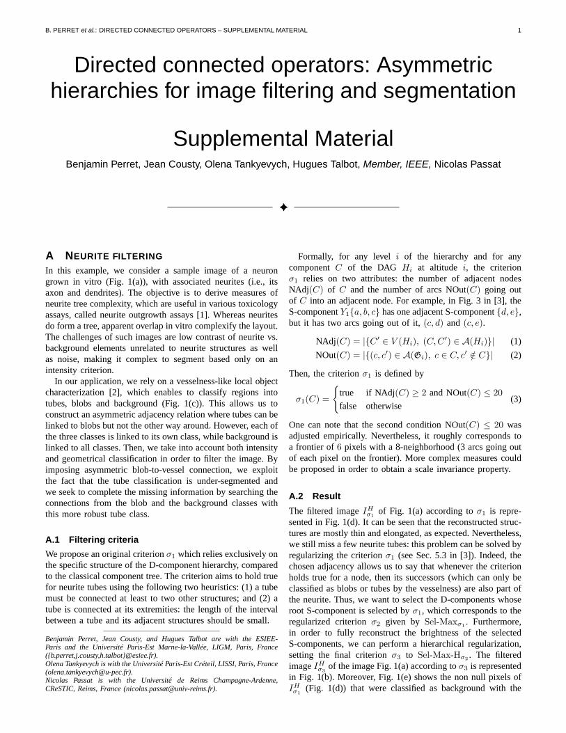
B. PERRET et al.: DIRECTED CONNECTED OPERATORS – SUPPLEMENTAL MATERIAL 1

Directed connected operators: Asymmetrichierarchies for image filtering and segmentation

Supplemental MaterialBenjamin Perret, Jean Cousty, Olena Tankyevych, Hugues Talbot, Member, IEEE, Nicolas Passat

✦

A NEURITE FILTERING

In this example, we consider a sample image of a neurongrown in vitro (Fig. 1(a)), with associated neurites (i.e., itsaxon and dendrites). The objective is to derive measures ofneurite tree complexity, which are useful in various toxicologyassays, called neurite outgrowth assays [1]. Whereas neuritesdo form a tree, apparent overlap in vitro complexify the layout.The challenges of such images are low contrast of neurite vs.background elements unrelated to neurite structures as wellas noise, making it complex to segment based only on anintensity criterion.

In our application, we rely on a vesselness-like local objectcharacterization [2], which enables to classify regions intotubes, blobs and background (Fig. 1(c)). This allows us toconstruct an asymmetric adjacency relation where tubes can belinked to blobs but not the other way around. However, each ofthe three classes is linked to its own class, while background islinked to all classes. Then, we take into account both intensityand geometrical classification in order to filter the image. Byimposing asymmetric blob-to-vessel connection, we exploitthe fact that the tube classification is under-segmented andwe seek to complete the missing information by searching theconnections from the blob and the background classes withthis more robust tube class.

A.1 Filtering criteria

We propose an original criterion σ1 which relies exclusively onthe specific structure of the D-component hierarchy, comparedto the classical component tree. The criterion aims to hold truefor neurite tubes using the following two heuristics: (1) a tubemust be connected at least to two other structures; and (2) atube is connected at its extremities: the length of the intervalbetween a tube and its adjacent structures should be small.

Benjamin Perret, Jean Cousty, and Hugues Talbot are with the ESIEE-Paris and the Université Paris-Est Marne-la-Vallée, LIGM, Paris, France({b.perret,j.cousty,h.talbot}@esiee.fr).Olena Tankyevych is with the Université Paris-Est Créteil, LISSI, Paris, France([email protected]).Nicolas Passat is with the Université de Reims Champagne-Ardenne,CReSTIC, Reims, France ([email protected]).

Formally, for any level i of the hierarchy and for anycomponent C of the DAG Hi at altitude i, the criterionσ1 relies on two attributes: the number of adjacent nodesNAdj(C) of C and the number of arcs NOut(C) going outof C into an adjacent node. For example, in Fig. 3 in [3], theS-component Y1{a, b, c} has one adjacent S-component {d, e},but it has two arcs going out of it, (c, d) and (c, e).

NAdj(C) = |{C ′ ∈ V (Hi), (C,C′) ∈ A(Hi)}| (1)

NOut(C) = |{(c, c′) ∈ A(Gi), c ∈ C, c′ /∈ C}| (2)

Then, the criterion σ1 is defined by

σ1(C) =

{

true if NAdj(C) ≥ 2 and NOut(C) ≤ 20

false otherwise(3)

One can note that the second condition NOut(C) ≤ 20 wasadjusted empirically. Nevertheless, it roughly corresponds toa frontier of 6 pixels with a 8-neighborhood (3 arcs going outof each pixel on the frontier). More complex measures couldbe proposed in order to obtain a scale invariance property.

A.2 Result

The filtered image IHσ1of Fig. 1(a) according to σ1 is repre-

sented in Fig. 1(d). It can be seen that the reconstructed struc-tures are mostly thin and elongated, as expected. Nevertheless,we still miss a few neurite tubes: this problem can be solved byregularizing the criterion σ1 (see Sec. 5.3 in [3]). Indeed, thechosen adjacency allows us to say that whenever the criterionholds true for a node, then its successors (which can only beclassified as blobs or tubes by the vesselness) are also part ofthe neurite. Thus, we want to select the D-components whoseroot S-component is selected by σ1, which corresponds to theregularized criterion σ2 given by Sel-Maxσ1

. Furthermore,in order to fully reconstruct the brightness of the selectedS-components, we can perform a hierarchical regularization,setting the final criterion σ3 to Sel-Max-Hσ2

. The filteredimage IHσ3

of the image Fig. 1(a) according to σ3 is representedin Fig. 1(b). Moreover, Fig. 1(e) shows the non null pixels ofIHσ1

(Fig. 1(d)) that were classified as background with the

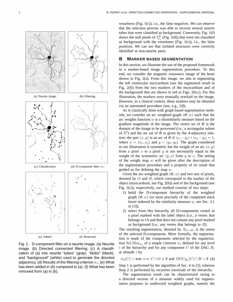
2 B. PERRET et al.: DIRECTED CONNECTED OPERATORS – SUPPLEMENTAL MATERIAL

(a) Neurite image. (b) Filtering.

(c) Classification. (d) D-component filter σ1.

(e) Added. (f) Removed.

Fig. 1. D-component filter on a neurite image. (a) Neuriteimage. (b) Directed connected filtering. (c) A classifi-cation of (a) into neurite “tubes” (gray), “blobs” (black),and “background” (white) used to generate the directedadjacency. (d) Results of the filtering criterion σ1. (e) Whathas been added in (b) compared to (a). (f) What has beenremoved from (a) in (b).

vesselness (Fig. 1(c)), i.e., the false negatives. We can observethat the selection process was able to recover several neuritetubes that were classified as background. Conversely, Fig. 1(f)shows the null pixels of IHσ1

(Fig. 1(d)) that were not classifiedas background with the vesselness (Fig. 1(c)), i.e., the falsepositives. We can see that isolated structures were correctlyidentified as non-neurite parts.

B MARKER BASED SEGMENTATION

In this section, we illustrate the use of the proposed frameworkin a marker-based image segmentation procedure. To thisend, we consider the magnetic resonance image of the heartshown in Fig. 2(a). From this image, we aim at segmentingthe left ventricular myocardium (see the segmented result inFig. 2(f)) from the two markers of the myocardium and ofthe background that are shown in red in Figs. 2(b,c). For thisillustration, the markers were manually overlaid on the image.However, in a clinical context, these markers may be obtainedvia an automated procedure (see, e.g., [4]).

As is classically done with graph based segmentation meth-ods, we consider an arc weighted graph (G, w) such that thearc weights function w is a dissimilarity measure based on thegradient magnitude of the image. The vertex set of G is thedomain of the image to be processed (i.e., a rectangular subsetof Z2) and the arc set of G is given by the 4-adjacency rela-tion: the pair (x, y) is an arc of G if |x1−y1|+ |x2−y2| = 1,where x = (x1, x2) and y = (y1, y2). The graph consideredin our illustration is symmetric but the weight of an arc (x, y)from a pixel x to a pixel y is not necessarily equal to theweight of the symmetric arc (y, x) from y to x. The settingof the weight map w will be given after the description ofthe segmentation procedure and a property of its result thatguided us for defining the map w.

Given the arc-weighted graph (G, w) and two sets of pixels,denoted by O and B, which correspond to the marker of theobject (myocardium, see Fig. 2(b)) and of the background (seeFig. 2(c)), respectively, our method consists of two steps:

1) build the D-component hierarchy of the weightedgraph (G, w) (or more precisely of the completed stacklower induced by the similarity measure w, see Sec. 3.1in [3]);

2) select from this hierarchy all D-components rooted ina pixel marked with the label object (i.e., a vertex thatbelongs to O) and that does not contain any pixel markedas background (i.e., any vertex that belongs to B).

The resulting segmentation, denoted by SO→B , is the unionof the selected D-components. More formally, the segmenta-tion is made of the components selected by the regulariza-tion Sel-Maxσ4

of a simple criterion σ4 defined for any leveli of the hierarchy and for any component C of the DAG Hi

at altitude i by

σ4(C) = true ⇐⇒ C ∩O �= ∅ and DCCHi(C)∩B = ∅ (4)

Step 1 is performed by the algorithm of Sec. 4 in [3], whereasStep 2 is performed by recursive traversals of the hierarchy.

The segmentation result can be characterized owing toa directed version of a measure widely used for segmen-tation purposes in undirected weighted graphs, namely the


(a) Original (b) O: myocardium (c) B: background (d) Symmetric result (e) S0: Over-seg (f) Directed result

Fig. 2. Segmentation based on the D-component hierarchy. (b,c,e) The considered sets are superimposed in red tothe original image. (d,f) The internal border of the segmentation results are superimposed in red to the original image.

connection value [5], [6] (also called degree of connectivity[7] or fuzzy connectedness [8] up to an inversion of w).If π = (x0, . . . , x�) is a path in G, the connection value Υw(π)of π is the maximum weight of the arcs of π

Υw(π) =

{

max{w(xi, xi−1), i ∈ [[1, �]]} if π non-trivial0 otherwise

(5)The (directed) connection value Υw(x, y) from a vertex x of Gto a vertex y is then defined as the minimum of the connectionvalues of the paths from x to y

Υw(x, y) = min{Υw(π), π is a path from x to y} (6)

Hence, by the very definition of a D-component hierarchy, itcan be shown that the segmentation result SO→B is the setof all vertices whose directed connection value from a vertexmarked as object is less than the one to a vertex marked asbackground, i.e., for any x ∈ V (G), we have

x ∈ SO→B ⇐⇒ mino∈O

{Υw(o, x)} < minb∈B

{Υw(x, b)} (7)

From the previous characterizations of the proposed seg-mentation method, we can say intuitively that the weightsof the arcs should be higher in the border of the object tobe segmented than inside and outside this object. In orderto produce such a map and, following the work of [9], theweight w(x, y) of the arc (x, y) is the product of a symmetricterm ∇(x, y) and a non necessarily symmetric term δ(x, y)

w(x, y) = ∇(x, y).δ(x, y) (8)

The first term ∇(x, y) plays the role of a gradient magni-tude. For our illustration, it is defined as the absolute differenceof intensity between the pixels x and y. If I denotes thegrayscale image to be segmented we have

∇(x, y) = |I(x)− I(y)| (9)

when no further knowledge on the objects to be segmentedexists, symmetric weights can be used. In this case the secondterm δ(x, y) is set to a constant value. For instance, the imageof Fig. 2(d) is obtained by the proposed method from themarkers O and B shown in Figs. 2(b,c) when a constant valueis used for the map δ.

However, when domain knowledge is available, the secondterm δ(x, y) can be used to ease the connection of a pixeleither to the background or to the foreground marker. FromEq. (7), we remark that if the weight of every arc (x, y)

ending at a vertex y is set to an infinite value (i.e., a maximalweight), then the vertex y does not belong to the segmentedobject SO→B . Indeed, in this case, the connection value fromany point o of the marker O to the vertex y is maximaland therefore, by Eq. (7), the vertex y does not belong tothe segmented object SO→B . On the other hand, when theweight of every arc starting at x is maximal (i.e., in the caseswhere the connection value from the object marker is notalso maximal), the point x generally belongs to the segmentedobject SO→B . These observations allow us to design a strategyto take into account some prior information in the arcs weightsin order to ease the connection of a given point either to thebackground marker or to object marker. Indeed, if we havegood confidence that a pixel x belongs to the object (but nothigh enough to put it in the object marker), we can increasethe weights of the arcs going out from x in order to harden itsconnection to the background. Conversely, if we are confidentthat a pixel x belongs to the background, we have to increasethe weights of the arcs ending in x.

Following this strategy, we set the term δ(x, y) in Eq. (8)based on a first classification of the image pixels that producesmany false positives but tends to minimize the false negatives.In other words, this classification tends to produce a superset,denoted by S0, of the expected segmentation result. In ourillustration, S0 is obtained by excluding the extremal intensityvalues, which correspond to blood and fat for the brightestpixels and to lungs for the darkest ones (see Fig. 2(e)). Hence,we are confident that the points that do not belong to S0 donot belong to the object that we seek to segment. Then, theterms {δ(x, y)} are set up in order to ease the connection of thepixels that do not belong to S0, to the background marker B.This is done by multiplying by a constant value the weight ofany arc (x, y) ending at a pixel classified as background

δ(x, y) =

{

1 if y /∈ S0

K otherwise(10)

where K > 1.The result of our method (with K = 1.5) for the my-

ocardium segmentation is presented in Fig. 2(f).

REFERENCES

[1] J. Bilsland, M. Rigby, L. Young, and S. Harper, “A rapid method forsemi-quantitative analysis of neurite outgrowth from chick DRG explantsusing image analysis,” J Neurosci Meth, vol. 92, pp. 75–85, 1999.

4 B. PERRET et al.: DIRECTED CONNECTED OPERATORS – SUPPLEMENTAL MATERIAL

[2] A. F. Frangi, W. J. Niessen, R. M. Hoogeveen, T. van Walsum, andM. A. Viergever, “Model-based quantitation of 3-D magnetic resonanceangiographic images,” IEEE T Med Imaging, vol. 18, pp. 946–956, 1999.

[3] B. Perret, J. Cousty, O. Tankyevych, H. Talbot, and N. Passat, “Di-rected connected operators: Asymmetric hierarchies for image filter-ing and segmentation,” IEEE T Pattern Anal, vol. 0. In Press. DOI:10.1109/TPAMI.2014.2366145, pp. 1–14, 2014.

[4] J. Cousty, L. Najman, M. Couprie, S. Clément-Guinaudeau, T. Goissen,and J. Garot, “Segmentation of 4D cardiac MRI: Automated method basedon spatio-temporal watershed cuts,” Image Vision Comput, vol. 28, pp.1229–1243, 2010.

[5] G. Bertrand, “On topological watersheds,” J Math Imaging Vis, vol. 22,pp. 217–230, 2005.

[6] J. Cousty, G. Bertrand, L. Najman, and M. Couprie, “Watershed cuts:Thinnings, shortest-path forests and topological watersheds,” IEEE TPattern Anal, vol. 32, pp. 925–939, 2010.

[7] A. Rosenfeld, “On connectivity properties of grayscale pictures,” PatternRecogn, vol. 16, pp. 47–50, 1983.

[8] J. K. Udupa and S. Samarsekara, “Fuzzy connectedness and objectdefinition: Theory, algorithms, and applications in image segmentation,”CVGIP-Graph Model Im, vol. 58, pp. 246–261, 1996.

[9] P. A. V. Miranda and L. A. C. Mansilla, “Oriented image forestingtransform segmentation by seed competition,” IEEE T Image Process,vol. 23, pp. 389–398, 2014.

Directed connected operators: Asymmetric hierarchies for ...

Documents

Transcript of Directed connected operators: Asymmetric hierarchies for ...