NASA Contractor Report 187537

!

ICASE Report No. 91-29

ICASEDIRECT SIMULATION OF COMPRESSIBLE

TURBULENCE IN A SHEAR FLOW

_-_ (NASA-CE-I_75R7) uIF_CT :gI[MULATIT_N UF

_--= CQMPRESSIT_LF TUP, BULFNCE IN _ SHFAR FLON

Fin31 Report:. (ICASF) 42 p CSCL 01A

NOl-ZO0_l

Unclas00072B0

S. Sarkar

G. Erlebacher

M. Y. Hussaini

Contract No. NAS1-18605

March 1991

Institute for Computer Applications in Science and Engineering

NASA Langley Research Center

Hampton, Virginia 23665-5225

Operated by the Universities Space Research Association

|i

ii

|ii

i!i!

m

fU/ /X.Nalinnml Ar, rona,jlicm and

Sl'_a_'e A(hninislralion

Lnngley Re._eArcfl Cenler

t-larnpton, Virginia 23665-5225

DIRECT SIMULATION OF COMPRESSIBLE TURBULENCE

IN A SHEAR FLOW a

S. Sarkar, G. Erlebacher, and M.Y. Hussaini

Institute for Computer Applications in Science and Engineering

NASA Langley Research Center

Hampton, VA 23665

ABSTRACT

The purpose of this study is to investigate compressibility effects on the turbulence in homo-

geneous shear flow. We find that the growth of the turbulent kinetic energy decreases with

increasing Mach number - a phenomenon which is similar to the reduction of turbulent ve-

locity intensities observed in experiments on supersonic free shear layers. An examination of

the turbulent energy budget shows that both the compressible dissipation and the pressure-

dilatation contribute to the decrease in the growth of kinetic energy. The pressure-dilatation

is predominantly negative in homogeneous shear flow, in contrast to its predominantly pos-

itive behavior in isotropic turbulence. The different signs of the pressure-dilatation are

explained by theoretical consideration of the equations for the pressure variance and density

variance. We obtained previously the following results for isotropic turbulence; first, the

normalized compressible dissipation is of O(M_), and second, there is approximate equipar-

tition between the kinetic and potential energies associated with the fluctuating compressible

mode. Both these results have now been substantiated in the case of homogeneous shear.

The dilatation field is significantly more skewed and intermittent than the vorticity field.

Strong compressions seem to be more likely than strong expansions.

1This research was supported by the National Aeronautics and Space Administration under NASA Con-tract No. NAS1-18605 while the authors were in residence at the Institute for Computer Applications in

Science and Engineering (ICASE), NASA Langley Research Center, Hampton, VA 23665.

1 Introduction

Homogeneous shear flow refers to the problem of spatially homogeneous turbulence sustained

by a parallel mean velocity field _ = (Sz2, O, O) with a constant shear rate S. Such a flow

is perhaps the simplest idealization of turbulent shear flow where there are no boundary

effects, and where the given mean flow is unaffected by the Reynolds stresses. Nevertheless,

the crucial mechanisms of sustenance of turbulent fluctuations by a mean velocity gradient,

and the energy cascade down to the small scales of motion are both present in this flow.

The homogeneous shear flow problem has been studied experimentally by Champagne,

Harris and Corrsin (1970), Harris, Graham and Corrsin (1977), and Tavoularis and Corrsin

(1981) among others. In these low-speed experiments the statistical properties of the flow

do not vary spatially in the transverse (x2, z3) plane but they evolve in the streamwise zl

direction. In theory, the streamwise inhomogeneity can be removed by writing the equations

of motion in a reference frame moving with the mean flow _. In the moving reference frame,

the one-point moments satisfy pure evolution equations in time clearly illustrating that ho-

mogeneous turbulence is fundamentally an initial value problem. Rogallo (1981) and Rogers

and Moin (1987) have investigated the incompressible homogeneous shear problem at great

depth through direct numerical simulations. These simulations, albeit at low turbulence

Reynolds numbers, have provided turbulence statistics which are in good agreement with

experiments performed at relatively higher Reynolds numbers. Furthermore, since the sim-

ulations provide global instantaneous fields, the turbulence can be studied in much greater

detail than in physical experiments.

Recently there has been a spurt of activity in the direct numerical simulation (DNS) of

three-dimensional compressible turbulence. Decaying isotropic turbulence has been studied

by Passot (1987), Erlebacher et al. (1990), Sarkar et al. (1989), and Lee, Lele and Moin

(1990). The simulations of Erlebacher et al. (1990) identified different transient regimes

including a regime with weak shocks, and also showed that a velocity field which is initially

solenoidal can develop a significant dilatational component at later times. Sarkar et al.

(1989) investigated the statistical moments associated with the compressible mode in their

simulations, and determined a quasi-equilibrium in these statistics for moderate turbulent

Mach numbers which was then used to model various dilatational correlations. Lee, Lele

and Moin (1990) studied eddy shocklets which developed in their simulations when the

initial turbulent Mach number was sufficiently high (Mr > 0.6). Kida and Orszag (1990)

primarily studied power spectra, and energy transfer mechanisms between the solenoidal and

dilatational components of the velocity in their simulations of forced isotropic turbulence.

Physical experiments have not been and perhaps cannot be performed for homogeneous

shear flows at flow speeds which are sufficiently high to introduce compressible effects on the

turbulence. However, direct numerical simulation of this problem could provide meaningful

data, especially since DN$ for the incompressible problem has been successful in giving

realistic flow fields. The compressible problem was considered by Feiereisen et al. (1982)

who performed relatively low resolution 643 simulations and concluded that compressibility

effects are small. Recently Blaisdell (1990) has also considered compressibIe shear flow.

We have performed both 963 and 1283 simulations which have allowed us to obtain some

interesting new results regarding the influence of compressibility on the turbulence. In

contrast to the results of Feiereisen et al., our simulations which start with incompressible

initial data develop significant rms levels of dilatational velocity and density. We find that

the growth rate of the kinetic energy decreases with increasing Mach number as well as

increasing rms density fluctuations and show that the compressible dissipation and pressure-

dilatation contribute to this effect. Apart from rms levels of the fluctuating variables, we

have also examined their probability density functions (pdf) and higher order moments. The

dilatational field has different skewness and flatness characteristics relative to the vorticity

field. In particular, the dilatational field has a significant negative skewness and is more

intermittent than the vorticity field.

2 Simulation Method

The compressible Navier-Stokes equations are written in a frame of reference moving with the

mean flow _1. This transformation, which was introduced by Rogallo (1981) for incompress-

2

ible homogeneous shear, removes the explicit dependence on _(x2) in the exact equations for

the fluctuating velocity, thus allowing the imposition of periodic boundary conditions in the

x2 direction. The relation between x_ and the lab frame xi is

3:1 = _1 -- S_X2 , X2 = X2 , X3 -_ 3:3

Here S denotes the constant shear rate u,,2. In the transformed frame z,*., the compressible

Navier-Stokes equations take the following form

a,p+ - = o (1)

(2)

! I

C_tp + Uj P,.i + "ypuj, j = Stu2'p, 1 + "yS_p_, 1

(3)

p= pRT (4)

where • = Tiju_,j is the dissipation function, ui _ the fluctuating velocity, p the instanta-

neous density, p the pressure, T the temperature, R the gas constant, and n the thermal

conductivity. The viscous stress is

2

where/_ is the molecular viscosity which is taken to be constant. All the derivatives in the

above system are evaluated with respect to the transformed coordinates x*.

Since Eqs. (1)-(4) do not have any explicit dependence on the spatial coordinates x_, and

because the homogeneous shear flow problem, by definition, does not have any boundary

effects, periodic boundary conditions are allowable on all the faces of the computational box.

Of course, in order to obtain realistic turbulence fields it is necessary that the length of the

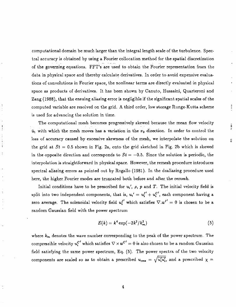
computational domain bemuch larger than the integral length scaleof the turbulence. Spec-

tral accuracyis obtained by usinga Fourier collocation method for the spatial discretization

of the governingequations. FFT's are usedto obtain the Fourier representationfrom the

data in physical spaceand thereby calculatederivatives. In order to avoid expensiveevalua-

tions of convolutions in Fourier space,the nonlinear terms are directly evaluatedin physical

spaceas products of derivatives. It has beenshownby Canuto, Hussaini, Quarteroni and

Zang(1988), that the ensuingaliasingerror is negligibleif the significant spatial scalesof the

computed variable are resolvedon the grid. A third order, low storageRunge-Kutta scheme

is usedfor advancingthe solution in time.

The computational meshbecomesprogressivelyskewedbecausethe mean flow velocity

fil with which the meshmoveshas a variation in the z2 direction. In order to control the

lossof accuracycausedby excessiveskewnessof the mesh, we interpolate the solution on

the grid at St = 0.5 shown in Fig. 2a, onto the grid sketched in Fig. 2b which is skewed

in the opposite direction and corresponds to St = -0.5. Since the solution is periodic, the

interpolation is straightforward in physical space. However, the remesh procedure introduces

spectral aliasing errors as pointed out by Rogallo (1981). In the dealiasing procedure used

here, the higher Fourier modes are truncated both before and after the remesh.

Initial conditions have to be prescribed for ui r, p, p and T. The initial velocity field is

It C tsplit into two independent components, that is, ui _ = u, + ui , each component having a

i Izero average. The solenoidal velocity field ul which satisfies V.u # = 0 is chosen to be a

random Gaussian field with the power spectrum

E(k) = k' exp(-2k2/k_) (5)

where k,_ denotes the wave number corresponding to the peak of the power spectrum. The

Ctcompressible velocity u i which satisfies V × u cl = 0 is also chosen to be a random Gaussian

field satisfying the same power spectrum, Eq. (5). The power spectra of the two velocity

components are scaled so as to obtain a prescribed u_ = , and a prescribed X =

4

Cu_/u=,, which is the compressible fraction of kinetic energy. The pressure pZ_ associated

with the incompressible velocity is evaluated from the Poisson equation

_2pl _ -- i I _ i I 11= --2pSu 2,1 --pu i,jU j,i (6)

It remains to specify the thermodynamic variables. The mean density p is chosen equal to

unity, and p is chosen so as to obtain a prescribed Mach number um_/_/-_'/_ characterizing

the turbulence. The fluctuating density p_ and compressible pressure pC_ are chosen as

random fields with the power spectrum Eq. (5) and prescribed p_ and vp_.,. The pressure

CIthen becomes p = _+ pI'+ p , the density is p = p+ p', and the temperature T is obtained

from the equation of state p = pRT.

3 Results

We have performed simulations for a variety of initial conditions and obtained turbulent fields

with Taylor microscale Reynolds numbers Re:_ up to 35 and turbulent Mach numbers Mt up

to 0.6. Note that Re_, = q)_/v where q = _ and k, = q� _, while Mt = q/-_ where

is the mean speed of sound. The computational domain is a cube with side 2_r. The results

discussed here were obtained with a uniform 963 mesh overlaying the computational domain.

The initial values of some of the important non-dimensional parameters associated with the

DNS cases ranged as follows: 3.6 < (SK/e)o < 7.2, 16 < Rea,o < 24, 0.2 < M_,0 < 0.4, and

0 < X < 0.15. We note that K denotes the turbulent kinetic energy and e the turbulent

dissipation rate.

In previous work by Erlebacher et al. (1990) on isotropic turbulence, it was found that for

a given initial Re_,, the initial choice of the non-dimensional quantities Mr, pr_/'_, T_n_/T,

p_.,/_ and X had a strong and lasting influence on the temporal evolution of the turbulence.

The different choices of initial conditions that lead to different regimes were classified by

Erlebacher et al. Even though the long time statistics in isotropic turbulence are, in general,

strongly dependent on the initial conditions, there is a quantity in isotropic turbulence which

has a large degreeof universality (in the absenceof shocks). This quantity is the partition

factor F defined by

which was shown by Sarkar et al.

F = .7_M_x/p_ (7)

(1989) to equal unity (to lowest order) in a low Mt

asymptotic analysis, and to approach unity from a variety of initial conditions in direct

simulations of isotropic turbulence with Mt up to 0.6. The physical interpretation of F ---* 1

is that there is a tendency towards equipartition between the kinetic energy and potential

energy of the compressible component of the turbulence.i:

In the case of initially isotropic turbulence subjected to homogeneous shear, for a given

initial energy spectrum, the solution of the incompressible equations depends on the ini-

tial conditions through the parameters (sK/e)o and Re_,,o. The compressible case depends

additionally on the initial levels of the thermodynamic fluctuations, dilatational velocity com-

ponent and turbulent Mach number. Apart from the influence of initial conditions, another

and perhaps more important feature is the influence of local compressibility and interactions

between the velocity and thermodynamic fields on the statistics at a given time. Equilibrium

scalings (if present) are also important to ascertain so as to improve the present capabilities

of modeling compressible turbulence. In order to address these issues, we present selected

results on second-order moments, pdf's (probability density functions), and hlgher-order

moments of both the velocity and thermodynamic fields.

3.1 Second-order moments

Evidence from physical and numerical experiments ( e.g., Tavoularis and Corrsin (1981) and

Rogallo (1981)) indicate that for incompressible homogeneous shear, both the turbulent

kinetic energy and the turbulent dissipation rate increase exponentially. Though our sim-

ulations are in accord with this picture of exponential growth, we note that Bernard and

Speziale (1990) have recently proposed an alternative picture where, after a substantially

long period of exponential growth, the turbulent energy eventually becomes bounded for

large St through a saturation induced by vortex stretching. In order to explore the effect

6

of initial levels of compressibility on the evolution of the turbulent statistics, we have per-

formed simulations based on two distinct types of initial conditions. The simulations of the

first type, whose results are shown in Figs. 3a-6a, start with incompressible data, that is,

pr_,0 = X0 = 0, but have different initial Mach numbers Mr,0. The second type of simula-

tions, whose results are shown in Fig. 3b-6b, start with different levels of initial rms density\

fluctuations rp,0 = (p_-,,/'_)o and compressible fraction of kinetic energy X0, but have the

same Mr,0 = 0.3. We note that all the cases of Figs. 3-6 have Rex,0 = 24 and (SK/E)o = 7.2.

The DNS results of Fig. 3a show that the level of the Favre-averaged kinetic energy K at

a given time decreases with increasing Mt,o in the simulations with the first type of initial

conditions, while Fig. 3b shows that the level of K also decreases with increasing X0 and rp,0

for the simulations with the second type of initial conditions. Thus an increase in compress-

ibility level, either due to increased Mach number or increased dilatational fraction of the

velocity field decreases the growth of turbulent kinetic energy in the case of homogeneous

shear flow. Fig. 4 shows that the development of the turbulent dissipation e has two phases.

In the first phase (S_ < 4) the higher compressibility cases have higher values of e probably

due to the buildup of the compressible dissipation e=. Later, in the second phase, the trend

reverses and the compressible cases have lower e relative to the incompressible case. Thus,

compressibility results in decreased growth of both e and K.

In order to explain the phenomenon of reduced growth rate of kinetic energy, we consider

the equation governing the kinetic energy of turbulence in homogeneous shear which is

d (-_K) = -Sp--u_'u'-'-"2'- "_e+ (8)

where _e is the turbulent dissipation rate and pld""7is the pressure-dilatation. The overbar

over a variable denotes a conventional Reynolds average, while the overtilde denotes a Favre

average. A single superscript ' represents fluctuations with respect to the Reynolds average,

while a double superscript " signifies fluctuations with respect to the Favre average. It was

shown in Sarkar et al. (1989) that the effect of compressibility on the dissipation rate can

7

be advantageously studied by using the decomposition

e = eo + ec (9)

-- J !where the solenoidal dissipation rate e, = uwiw i and the compressible dissipation rate e¢ =

(4/3)_-d '2. Here w_ denotes the fluctuating vorticity and d' denotes the fluctuating divergence

of velocity. We note that the correlations involving the fluctuating viscosity have been

neglected on the rhs of Eq. (9). Substituting Eq.(9) into Eq.(8) gives

d . .__.,--_(fig) = ,S-_wiu 2 - -_eo - "_ec + _ (10)

and the last two terms represent the explicit influence of the non-solenoidal nature of the

fluctuating velocity field in the kinetic energy budget. The DNS time histories for ec and

are presented in Figs. 5-6 respectively. The compressible dissipation e_ is always positive (as

expected) and when starting from a zero initial value as in Fig. 5a shows a monotonic increase

with time. The pressure-diiatati0n/-d' is highly oscillatory as seen in Fig. 6. Though p'd'

can be both positive or negative it tends to be predominantly negative. The tendency of

to be negative in homogeneous shear is clearly shown in Fig. 7 where the oscillations are

smoothed out by plotting values of _ obtained by averaging over successive time intervals.

Interestingly enough, on comparing Figs. 5a and 7a it seems that the time averaged values

of -p'd' and e_ are of the same order and exhibit similar trends of increase with St and Mr,0.

These DNS results along with the kinetic energy equation (10) show that both e_ and p'd"-'_

have a dissipative effect on the turbulent kinetic energy.

The predominantly negative values of _ in homogeneous shear is in contrast to the

predominantly positive values reported in Sarkar et al. (1989) for the case of decaying

isotropic turbulence. To understand this contrasting behavior of p'd' we write the exact

equation for the pressure variance which is applicable to both these flows

d--_-_-_p = -27_p'd'- (27- 1)p'p'd'- 2% + ep (11)

where ep is a term depending on mean viscosity and mean conductivity which is negligible

compared to ep. Here ep = (7- 1)Rgp-T,_T_ and can be called the pressure dissipation

term by virtue of being a sink on the rhs of Eq. (11). Comparing Eq. (10) and Eq. (11) it

is clear that p'd' acts to transfer energy between the kinetic energy of turbulence _K and

the potential energy of the turbulence pa/(27p ). In the case of homogeneous shear the rms

values of the velocity and pressure increase with time. Now, the third term on the rhs of

Eq. (11) is always negative and therefore a sink for the pressure variance. For small p'/p we

can neglect the second term on the rhs of Eq. (11) with respect to the first term. Therefore

for p,2 to increase with time, a source term is necessary which implies that p'd' be negative

in accord with the DNS results. We note that a similar analysis of the equations for p,2 and

T'---_-indicate that p'd"--7and T'd' also have to be predominantly negative in this flow.

In decaying isotropic turbulence pa has to decay with time; however, because ev is suffi-

cient to ensure decay of p,---Tthe sign of pT-d7cannot be determined from Eq. (11). Alternatively,

we consider the exact density variance equation which for homogeneous shear flow is

(12)

For small p'/p, the first term on the rhs of Eq. (11) dominates the second term. Therefore

for pa to decrease with time it is necessary that p'd--7 be predominantly positive. If we

assume that the thermodynamic fluctuations are approximately isentropic in this case (DNS

supports this assumption), it immediately follows that p'd--7 is also predominantly positive

in decaying isotropic turbulence. Thus, the role of p'd' as a mechanism for energy transfer

between the kinetic energy and potential energy dictates its differing signs in homogeneous

shear and unforced isotropic turbulence.

Fig. 8a shows the temporal evolution of Mt for different choices of the initial values for

Mt and Rex. For all the cases, the turbulent Mach number shows a monotonic increase

with time for the range of St spanned by the simulations. Two results of the analysis of

Sarkar et al. (1989) which were validated previously in isotropic turbulence are now checked

in homogeneous shear flow. These results are, first, the compressible dissipation obeys the

scaling Q/Co = aM_, and second, the partition factor F _- 1 (see Eq. (7) for the definition of

F) which implies a tendency toward equipartition between the kinetic and potential energies

9

of the fluctuating compressible mode. Fig. 9a shows that for a variety of DNS cases the

ratio ec/(e,M2t) approaches an equiIibrium value of approximately 0.5 for large enough St.

The same ratio is plotted as a function of local Mt in Fig. 9b. Thus Fig. 9 supports our

previously derived result on the dependence of the compressible dissipation on turbulent

Mach number. Zeman (1989) had proposed the scaling Ec/E, = 1 -- exp{[(Mt -- 0.1)/0.6] 2}

which is clearly in contradiction with the DNS results of Fig. 9. The partition factor F is

seen in Fig. 10a to approach and oscillate around an equilibrium value of approximately 0.95

indicating that equipartition in the energies associated with the compressible mode holds in

the case of homogeneous shear too. In Fig. 10b we show the behavior of FT = 72M2tx/pa

which is defined using the total pressure variance rather than the compressible pressure

variance appearing in the definition of F. The parameter FT also appears to reach values

independent of initial conditions, however this trend is less pronounced in FT relative to F.

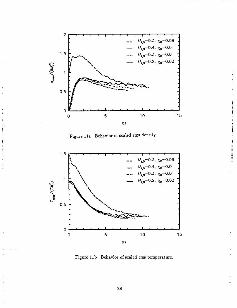
In Fig. 11 we show the time evolution of rms density and temperature fluctuations. It

appears that both the rms normalized density and temperature fluctuations eventually scale

as Mt 2. The rms pressure also scales as Mt 2. Erlebacher et al. (1990) decomposed the pressure

p into an incompressible component p_ and a compressible component pC. The behavior of

c and rp_, p,=, is shown in Fig. 12. The instantaneous incompressible pressure pt' satisfies

the Poisson equation Eq. (6). The compressible pressure pC' = p, _ pI' is the remaining

part of the pressure which arises from both density variations and non-zero divergence of the

velocity. Fig. 12 indicates that the rms of both components of the normafized pressure vary

like Mt 2. A simple order of magnitude analysis of Eq. (6) along with recognition of the fact

that SK/e = O(1) shows that p[=J_ = O(M2t). Thus it seems that in homogeneous shear

the conventionally accepted Mach number variation holds for I c andPr_,, Prm_ P_"

The evolution of pC' in the case where the initial data is incompressible can be understood

by considering the following equation for compressible pressure (see Erlebacher et al. (1990)

for details) where heat conduction and viscous effects have been neglected

I t C t C t C t C t I t C t" Ct i t it,,OtPc' + ui P ,i + ui P ,i + ui P ,i + '7(1 + p )ui,i --(Otp t' + ui P ,i) (13)

=

I0

C ISince pC' and u i are initially zero the growth ofp c_ is due to the forcing by the incompressible

pressure on the rhs of Eq. (13). This forcing causes p_/_ to become O(p_/_) = O(M'_) on

the convective time scale which explains the trend seen in the three lower curves of Fig. 12b.

c and cThe top curve of Fig. 12b, which corresponds to a case with initially non-zero Pr_ U_,,

also shows the same trend indicating that the forcing by the incompressible velocity field

(through pZ ) has a substantial influence in determining the level of pC_.

3.2 Probability density functions and higher order moments

The probability density function (pdf) gives a comprehensive description of a fluctuating

variable because it formally enables the calculation of all the statistical moments. Second-

order moments (discussed in the previous section) are probably the most important statistical

indicators of the turbulence because they characterize intensities and cross-correlations of the

fluctuating variables. Higher-order moments such as the skewness and flatness give additional

information on the statistical distribution of the variable, for example, a positive skewness

indicates a pdf which is skewed towards positive fluctuations from the mean, while a large

flatness indicates a large propensity for the occurrence of extreme values of the variable. The

skewness Sk(O) and flatness Fl(O) of a variable 0 are defined by

0, 3sk(0) =

(0,2)3/,0 '4

El(O) =(o,2)2

A quantity with a Gaussian pdf has Sk = 0 and Fl = 3. In this section, we present results on

pdf, skewness and flatness of some variables for a DNS case with significant compressibility

levels. The initial nondimensional parameters for this case are

Re_,=24 , SK/e=7.2 , Mr=0.4 , X--'O , pn._/-_=O , pV /_=0

The pdf f_, of the streamwise fluctuating velocity in Fig. 13a appears to be symmetric

around the origin. The skewness and flatness of u have insignificant deviations from Gaussian

11

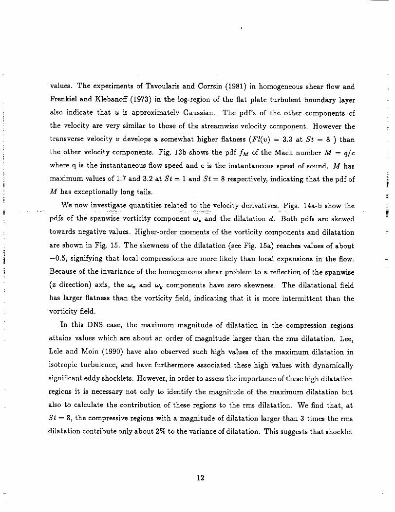
values. The experimentsof Tavoularisand Corrsin (1981) in homogeneousshearflow and

Frenkiel and Klebanoff (1973) in the log-regionof the flat plate turbulent boundary layer

also indicate that u is approximately Gaussian. The pdf's of the other components of

the velocity are very similar to those of the streamwise velocity component. However the

transverse velocity v develops a somewhat higher flatness (Fl(v) = 3.3 at St = 8 ) than

the other velocity components. Fig. 13b shows the pdf fM of the Mach number M = q/c

where q is the instantaneous flow speed and c is the instantaneous speed of sound. M has

maximum values of 1.7 and 3.2 at St = 1 and St = 8 respectively, indicating that the pdf of

M has exceptionally long tails.

We now investigate quantities related to the velocity derivatives. Figs. 14a-b show the

pdfs of the spanwise vorticity component wz and the dilatation d. Both pdfs are skewed

towards negative values. Higher-order moments of the vorticity components and dilatation

are shown in Fig. 15. The skewness of the dilatation (see Fig. 15a) reaches values of about

-0.5, signifying that local compressions are more likely than local expansions in the flow.

Because of the invariance of the homogeneous shear problem to a reflection of the spanwise

(z direction) axis, the wx and wv components have zero skewness. The dilatational field

has larger flatness than the vorticity field, indicating that it is more intermittent than the

vorticity field.

In this DNS case, the maximum magnitude of dilatation in the compression regions

attains values which are about an order of magnitude larger than the rms dilatation. Lee,

Lele and Moin (1990) have also observed such high values of the maximum dilatation in

isotropic turbulence, and have furthermore associated these high values with dynamically

significant eddy shocklets. However, in order to assess the importance of these high dilatation

regions it is necessary not only to identify the magnitude of the maximum dilatation but

also to calculate the contribution of these regions to the rms dilatation. We find that, at

S_ -= 8, the compressive regions with a magnitude of dilatation larger than 3 times the rms

dilatation contribute only about 2% to the variance of dilatation. This suggests that shocklet

12

dissipation is not the dominant contributory mechanismto the compressibledissipationfor

Mt < 0.5.

From Fig. 16a it appears that the imposition of shear does not alter the skewness and

flatness of the Mach number M appreciably from the isotropic turbulence values at S_ = 0.

The fact that M is bounded from below and not from above may be responsible for the

departure of skewness and flatness from Gaussian values. The instantaneous values of M

can become rather large ( the ratio Mm_x/Mt = 5.8 at S_ = 8), but the flatness level of 4

at S_ = 8 indicates that these large extrema have a relatively low probability of occurrence.

The long tall in the pdf of M (see Fig. 13b and the previous discussion of the figure) does not

seem to contribute significantly at the level of third and fourth moments. Fig. 16b shows that

the velocity field can be highly supersonic (M_x = 3.3 at St = 8). Though the percentage

of the volume occupied by supersonic fluctuations, denoted by ¢,uper in Fig. 16b, increases

with time, its maximum value is a modest 4.9% at St = 8.

4 Characteristics of the instantaneous flow

The previous sections have focused on the influence of compressibility on the statistical

attributes of homogeneous shear turbulence. We now present some preliminary results on

the spatial characteristics of the instantaneous turbulence from ongoing flow visualization.

Figs. 17-20 are results from the flow field at S_ = 9 for a case which has the following initial

nondimensional parameters

Re_=21 , SK/e=5.8 , Mr=0.3 , X=0.09 , p_.,_/'_=0.09 , pC /_=0.13

By St = 9 the initially isotropic turbulence develops into a realistic representation of ho-

mogeneous shear turbulence. The turbulence at St = 9 has Mt = 0.42, p_.,/-_ = 0.12 and

= 0.06, which implies a moderate level of compressibility, and has a Re_ = 32. One of

the important characteristics of the velocity field is the extent and topology of supersonic

regions. Fig. 17 shows a 3-D contour plot of regions with fluctuating Mach number M > 1.

These regions of supersonic fluctuations are small discrete regions scattered through the flow

13

domain, and are elongated in the streamwise direction. The volume occupied by the regions

with supersonic fluctuations is small. Fig. 18 shows the dilatation V.u' in a plane parallel

to the (xl, z2) plane. The regions in black are expansion regions with positive dilatation,

while the regions in grey and white are compression regions with negative dilatation. Both

the Compression reg_0ns and the expansion regions are very elongated in the streamwise zl

direction. The white portions in the dilatation plot of Fig. 18 correspond to compression

regions where the magnitude of dilatation is larger than the maximum positive dilatation.

The magnitude of dilatation in these white regions areupto 50% larger than the maximum

positive dilatation indicating that compressions are stronger than the expansions. As Fig. 18

shows, the white regions of strong compression are small and discrete elements which occupy

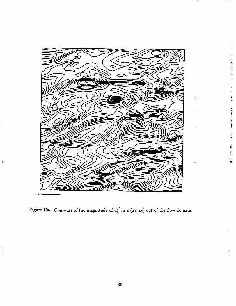
I Ia small portion of the plane. Figs. 19a and 19b are contour plots of the magnitude of u_ and

Ctui respectively in a plane parallel to the (zl, z2) plane. Regions with large gradients seem

C t ]-Ito be more prevalent in the u_ field relative to the u_ field. Figs. 20a and 20b show the

incompressible pressure pZ' and the compressible pressure pO' in the same plane considered' L

in Fig. 19. It is clear that the pZ' field has significant differences with respect to the pC' field.

The compressible pressure has higher gradients and more pronounced small scale features

than the incompressible pressure. Elongated and inclined structures are also visible in the

pO' field.

E

5 Conclusions

We have performed direct numerical simulations of homogeneous shear flow using a spectral

collocation technique and analyzed the data base in order to quantify compressibility effects

on the turbulence. An increase in the compressibility level (i.e. turbulent Mach number,

density fluctuations or rms dilatational velocity fluctuations) leads to a decrease in the

growth of turbulent kinetic energy. In the compressible case, the kinetic energy equation

has two additional terms, the compressible dissipation and the pressure-dilatation. Both

these terms have a dissipative contribution in shear flow, leading to the reduced growth of

the turbulent kinetic energy. The O(M_) variation of the compressible dissipation which

14

was obtained previously by an asymptotic theory and then verified in the DNS of isotropic

turbulence, has now been substantiated by the DNS of homogeneous shear turbulence. The

pressure-dilatation is a more difficult term to characterize, because it can be either positive

or negative and also because gradient transport arguments are clearly inapplicable. Our DNS

show that the pressure-dilatation is predominantly negative in the homogeneous shear case

in contrast to its predominantly positive character in decaying isotropic turbulence. Analysis

shows that, in the transport equation for the pressure variance, the pressure-dilatation has

to be a source in the case of homogeneous shear (where the turbulence grows) and a sink

in the case of decaying isotropic turbulence, thus accounting for the opposite signs of the

pressure-dilatation in the two flows. In the core region of inhomogeneous aerodynamic flows,

perhaps the pressure-dilatation is predominantly negative so as to transfer energy from the

velocity field to the pressure field.

It is well known that, for low-speed flows, the rms pressure normalized by the mean

pressure varies as O(M_). Our DNS results support this scaling of the rrns of pressure,

density and temperature fluctuations for compressible homogeneous shear flow. These DNS

results and our analysis suggest that such a scaling may be valid for those inhomogeneous

flows where the thermodynamic fluctuations arise due to high-speed effects and not due

to other factors such as external heating or cooling, and mixing of fluids with different

densities or temperatures. We have studied the probability density functions and higher-

order moments of the dilatation and the vorticity. The dilatation field has appreciable

negative skewness indicating a preponderance of compressions over expansions, and has a

larger flatness than the vorticity indicating that it is more intermittent than the vorticity.

The intermittent regions of negative dilatation were found to have only a small contribution

to the compressible dissipation for Mt < 0.5.

Acknowledgements

On the occasion of John Lurnley's 60th birthday, SS is pleased to thank John for teaching

him turbulence and motivating him to pursue research in the field of turbulence. The authors

15

wish to thank Tom Gatski and Charles Speziale for their comments on a preliminary draft

of this manuscript, and Tom Zang for helpful discussions.

16

References

Bernard, P.S., and Speziale, C. G. (1990) Bounded Energy States in Homogeneous

Turbulent Shear Flow - An Alternative View. ICASE Report No. 90-66, submitted to

Phys. Fluids A.

Blaisdell, G.A., Reynolds, W.C., Mansour, N.N., Zeman, O., and Aupoix, B. (1990)

Growth of Turbulent Kinetic Energy in Compressible Homogeneous Turbulent Shear

Flow. _3rd Annual Meeting of the APS/Division of Fluid Dynamics, Cornel] Univer-

sity, N.Y. ( November 1990).

Canuto, C., Hussaini, M.Y., Quarteroni, A., and Zang, T.A. (1988) Spectral Methods

in Fluid Dynamics. Springer-Verlag, Berlin.

Champagne, F.H., Harris, V.G., and Corrsin, S. (1970). Experiments on Nearly Ho-

mogeneous Turbulent Shear Flow. J. Fluid Mech., 41, 81.

Erlebacher, G., Hussaini, M.Y., Kreiss, H.O., and Sarkar, S. (1990) The Analysis and

Simulation of Compressible Turbulence. Theoret. Comput. Fluid Dynamics, 2, 73.

Feiereisen, W.J., Shirani, E., Ferziger, J.H., and Reynolds, W.C. (1982) Direct Simula-

tion of Homogeneous Turbulent Shear Flows on the Illiac IV Computer: Applications to

Compressible and Incompressible Modelling. In Turbulent Shear Flows 3, pp. 309-319.

Springer-Verlag, Berlin.

Frenkiel, F.N., and Klebanoff, P.S. (1973) Probability Distributions and Correlations

in a Turbulent Boundary Layer. Phys. Fluids, 16, 725.

Harris, V.G., Graham, J.A.H., and Corrsin, S. (1977). Further Experiments in Nearly

Homogeneous Turbulent Shear Flow. J. Fluid Mech., 81,657.

17

Kida, S. and Oszag, S.A. (1990). Energy and Spectral Dynamics in Forced Compress-

ible Turbulence. Submitted to J. Fluid Mech.

Lee, S., Lele, S.K., and Moin, P. (1990) Eddy-shocklets in Decaying Compressible

Turbulence. CTR Manuscript 117.

Passot, T. (1987). Simulations numeriques d'ecoulements compressibles homogenes en

regime turbulent : application aux nuages moieculaires. Ph. D. Thesis, University of

Paris.

Rogallo, R.S. (1981). Numerical Experiments in Homogeneous Turbulence. NASA TM

81315 .....

Rogers, M.M., and Moin, P. (1987). The Structure of the Vorticity Field in Homoge-

neous Turbulent Flows. J. Fluid Mech., 176, 33.

Sarkar, S., Erlebacher, G., Hussaini, M.Y., and Kreiss, H.O. (1989) The Analysis and

Modeling of Dilatational Terms in Compressible Turbulence. ICASE Report No. 89-7g,

J. Fluid Mech (in press).

Tavoularis, S., and Corrsin, S. (1981). Experiments in Nearly Homogeneous Turbulent

Shear Flow with a Uniform Mean Temperature Gradient. J. Fluid Mech., 104, 311.

18

X2

X1

Figure 1 Schematic of homogeneous shear flow.

X2 X2

X 1 b X'_a

Figure 2 Schematic of regrid procedure.

19

8

6

",: 4

Mr,o--O.4

2

.... Mr,o=0.2-- Mt,o=O

0 a_ I , I .... , I • I ,

2 4 6 80 10

St

Y.

6

5

4

0 15

" I • I / '

/

ee_ ,B@

/...:;'"/ .-';"

.... Xo=O. , Tp=O.09

__ Xo=O, rp=O

, I , I ,

5 10

St

Figure 3 Evolution of kinetic energy for various DNS cases.

2O

20

15

'_ 10

5

00 2 4 6 8 10

S_

14

oBoB°°o°

o o

s °

o ° •

__..°'2 s-

"'""_;°_"2"°""--- Xo=O- 15,.::.:: .".",_" "_'- .-_, Tp=0.1 1

.r_ .... xo=O.og, rFo.o9

_. Xo=O, rp=O

I I I I •

12

I0

8

6

4

0 5 10 15

St

Figure 4 Evolution of dissipation for various DNS cases.

21

1.5

0

=

2

1.5

o

0.5

0

0

Qg_

oo_l

m

' I

Mr,o=0.4

Mr,o=0.3

Mr,o=0.2

' I ' I ' I '

a °s °

oS

_o S

S._., S°S" ,'°

BS _ oB_ °B°

## : oeB

BS Bf o° _

e J ,n_ U _

BS B_ ° _

oS ooo _

jm oeo _

2 4 6 8 10

St

" I " I "

, \ b

i \

/',.. /

• • "°°..o o_o oo - XD _

...._ Xo=O, rp=o

, .-', ,0 5 10 15

St

Figure 5 Evolution of compressible dissipation for various DNS cases.

22

4 ' I " I '

0

-2

-4

-6

a

IIII

I

Mr,o=0.4

/_t,o=0.3

Mr,o=0.2

, I

5

, I ,

10

St

15

4

2

' I ' I '

b

o,., _,!]_ .

-=L .... _°=°'°_'T°'°o " W"__ Xo=O.,-.=o V

-40 5 10 15

St

Figure 6 Evolution of pressure-dilatation for various DNS cases

23

0.5 ' I ' I ' I ' I

1

f_

0.0

-0.5

-1.0

0.5

0.0

-0.5

-1.0

-1.5

\ .........

._. '.-..:_i.'\-- Mr,o=0.2 " _.

-%, i I , , ,l i I i,, I

2 4 6 8

St

• ! • ! ,

\' _ _ _-'"

.... xo=O.O9, ro=o.o9 \-- Xo=O, rp=O

, I j l

5 I0

St

i

110

=

i

15

Figure 7 Evolution of time-averaged pressure-dilatation for various DNS cases

24

0.6 I , , • I

[ ""0.5 _ "_S_'_ _'_ ._._"

I ..." ._.._.."" .-"

0.4 F_'-'_ _ _ _ o.° _o. _

0.3

0.2

0.1

0

oO_

O° o _OOO O0 °

a

! I |

0 5

_. Rx,o=16

-- Rx,o=24

.-. Rx,o=20

.... Rx,o=24

Rx,o=24

I i

10

St

15

0.6

0.5

0.4

0.3

0.2

0.1

' I " I

o- °-." oo: "o o o

b

0 , I0 5 15

._. Xo=0.15, to=0.11

.... Xo=O.09, rp=O.09

m xo=O, ,-p=oI

10

St

Figure 8 Evolution of turbulent Mach number for various DNS cases.

25

i

i

i

7.

i

=

la/

o

00,1

6

Figure 9

0.5 0,6

Behavior o{ scaled compressible dissipation.

26

1 .8 ' I ' I '

1.6 f a1.4

1 :l "" " ,,

0.8

0.6

0.4 I0.2

0 I i I , I ,

0 5 10 15

St

0.8

0.6 ¢"

0.4

0.2

' I ' I

,_wlo m -- _o

/'; b

I ;

I

0 5 10 15

St

Figure 10 Behavior of the partition parameters F and FT.

27

f

-- Mt, o=0.3, Xo=O.O9

.-. Mt,o=O.4, Xo=O.O

1.5 .... Mr,o=0.3 ' Xo=O.O

,,,""_ if'"--'- N- -- Mt.o=0.2, Xo=O.03

0.5

0 • ' I I _

0 5 10 15

S_

Figure lla Behavior of scaled rms density.

i __ Xo=O.09

.-. Mr.o=0.4, Xo=O.O

.... Mr,o=0.3, Xo=O.O

_ ,oo .xooo,1"\

0 5 10 15

St

Figure llb Behavior of scaled rms temperature.

28

2.0 •

v 1.0

i I ' I

-- Mt,o=0.3, Xo=O.09

.-. Mr,o=0.4, Xo=O.O

1.5 .... Mr,o=0.3, Xo=O.O

Mr,o=0.2, Xo=O.03

0.5 ,_.,.

0.0 , I i I ,

0 5 10 15

St

Figure 12a Behavior of scaled rms incompressible pressure.

2.0

1.5

' I

"_w %%

!

Re

.QIo

m

| I

Mt,o=O.5, Xo=O.09

Mr,o=0.4, Xo=O.O

Mt,o=O.3, Xo=O.O

Mr,0=0.2, X0=0.03

I ,m_ _ %e,,___% "1•_=k -: ""t /,."+%_- t

o.=I ,P/ I

0.0

0 5 10 15

St

Figure 12b Behavior of scaled rms compressible pressure.

29

!=

0.08

0.06

0.04

0.02

0.00-10

.... St=1.0m St=8.0

-5 o 5

U

10

Figure 13a Pdf of streamwise velocity.

0.10 =' _ ,-I

0.08 -

0.06 -

0.04 -

0.02

0.00 '0 1

| |

I

2

M

| i

.... St= 1.0St=8.0

| |

3 4

Figure 13b Pdf of Mach number.

3O

0.10

0.08

0.06

0.04

0.02

0.00

' I ' I " I ' I " ! ' I " i • I " I '

.... St= 1.0__ St=8.0

I i • J. L

-100 -80 -60 -40 -20 0 20 40 60 80 100

Figure 14a Pdf of spanwise vorticity component.

0.4

0.3

0.2

0.1

0.0-60

• 1 • ! ' I ' ! ' ! '

.... St=l .0__ S_=8.0

|

-4O -2O 0

d

| •

20 40 6O

Figure 14b Pdf of dilatation.

31

o6f t0.4 _z

(.,O z

0.2 d

0.0

-0.2

-0.4

-0.6

-0.8

0 2 4- 6 8 10

St

Figure 15a Skewness of vorticity components and dilatation.

(/1

t-

O

b-

10

8

4

• ! , I ' I ' !

_m

_ dr'lm_'_'_'_ '' '_ _.h_, -.o .... o..._...i_ _ f L

_y

_x

6.1 z

d

2 , I t ! t ! . I ,

0 2 4 6 8 10

St

Figure 15b Flatness of vorticity components and dilatation.

32

4

3

2

1

' I ' I ' I ...2 .......

0 , i0 2

....FL(M)

__ s (M)

Figure 16a

n I n I n

4 6 8

St

Skewness and flatness of Mach number.

Figure 16b

5

4

3

2

0

• I ' I ' I ' ._..m= _?'n_Lz

i

i i I i I , I ,

0 2 4 6 8

St

Maximum Mach number and volume fraction of supersonic fluctuations.

33

Figure 17 Perspective of supersonic regions in the flow.

34

Figure 18 Dilatation field in a (xl, _2) cut of the flow domain.

35

iz

Figure 19a Contours of the magnitude of u_' in a (Xl, _g2) cut of the flow domain.

36

C I

Figure 19b Contours of the magnitude of u_ in the plane shown in Fig. 19a.

37

Figure 20a Contours of pI' in the plane shown in Fig. 19a.

38

Figure 20b Contours of p cl in the plane shown in Fig. 19a.

39

N/iS6

1. Report NO.

NASA CR-1875 37

ICASE Report No. 91-29

4. Title and Subtitle

Report Documentation Page

2, Government Accession No.

DIRECT SIMULATION OF COMPRESSIBLE TURBULENCE IN A

SHEAR FLOW

7, Author(s)

3. Recipient's Catalog No.

5. Report Date

March 1991

6, Performing Organization Code

8. Performing Organization Report No.

91-29S. Sarkar

G. Erlebacher

M. Y. Hussaini

9. Performing Organization Name and Address

Institute for Computer Applications in Science

and Engineering

Mail Stop 132C, NASA Langley Research Center

Hampton, VA 23665-522512. Spon_ring Agency Name and Addre_

National Aeronautics and Space Administration

Langley Research Center

Hampton, VA 23665-5225

10. Work Unit No,

505-90-52-01

11, Contract or Grant No.

NASl-18605

13. Tyloe of Report and Period Covered

Contractor Report

14. Sponsoring Agency Code

15. Supplementaw Notes

Langley Technical Monitor:Michael F. Card

Submitted to Theoretical and Compu-

tational Fluid Dynamics.

Final Report16• Abstract

The purpose of this study is to investigate compressibility effects on

the turbulence in homogeneous shear flow. We find that the growth of the turbulent

kinetic energy decreases with increasing Mach number - a phenomenon which is similar

to the reduction of turbulent velocity intensities observed in experiments on super-

sonic free shear layers. An examination of the turbulent energy budget shows that

both the compressible dissipation and the pressure-dilatation contribute to the de-

crease in the growth of kinetic energy. The pressure-dilatatlon is predominantly

negative in homogeneous shear flow, in contrast to its predominantly positive behav-

ior in isotropic turbulence. The different signs of the pressure-dilatatlon are ex-

plained by theoretical consideration of the equations for the pressure variance and

density variance. We obtained previously the following results for Isotropic tur-

bulence; first, the normalized compressible dissipation is of O(M_), and second,

there is approximate equipartition between the kinetic and potential energies asso-

ciated with the fluctuating compressible mode. Both these results have now been sub-

stantiated in the case of homogeneous shear. The dilatation field is significantly

more skewed and intermittent than the vorticity field. Stong compressions seem to be

mo_e likely than s_ron_ exp_n_on_.17, Key Words(Suggest_ byAuthoHs)) 18. D_tributionStatemen!

02 - Aerodynamicsturbulence, compressible fluids, direct

numerical simulations

19. Securiw Cla_if (of this repot)

Unclassified

Unclassified - Unlimited

_. SecuriW Classif. (of this pagel 21 No+ of Da_s

Unclassified 41

NASA FORM I_ OCT 86

NASA-Langley, 199l

=