Direct Numerical Simulation of Pressure Fluctuations Induced by Supersonic Turbulent

Boundary Layers

PI: Lian Duan --- NSF PRAC 1640865- --- Missouri U. of S&T

1BlueWatersSymposium–2017Sunriver,OR,USA,May16-19,2017

Project Members: Chao Zhang, Junji Huang, Ryan Krattiger

2

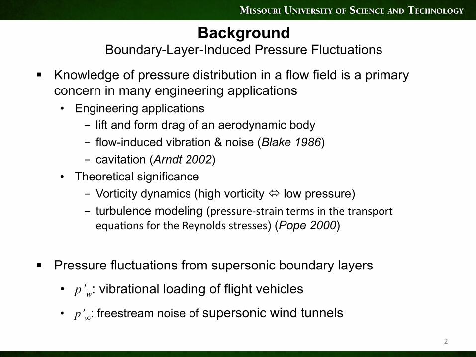
Background Boundary-Layer-Induced Pressure Fluctuations

§  Knowledge of pressure distribution in a flow field is a primary concern in many engineering applications •  Engineering applications

-  lift and form drag of an aerodynamic body -  flow-induced vibration & noise (Blake 1986) -  cavitation (Arndt 2002)

•  Theoretical significance -  Vorticity dynamics (high vorticity ó low pressure) -  turbulence modeling (pressure-straintermsinthetransportequaConsfortheReynoldsstresses) (Pope 2000)

§  Pressure fluctuations from supersonic boundary layers

•  p’w: vibrational loading of flight vehicles

•  p’∞: freestream noise of supersonic wind tunnels

3

Flow

LaminarTunnel-WallBoundaryLayer

UpstreamDisturbance

TurbulentTunnel-WallBoundaryLayerTransiCon

TestRhombusAcous*cRadia*on

ShadowgraphoftheradiatednoisefromaMach3.5tunnel-wall

turbulentboundarylayer(courtesyofNASA

Langley)

In a conventional tunnel (M∞ > 2.5), tunnel noise is dominated by acoustic radiation from turbulent boundary layers on tunnel side-walls (Laufer, 1964)

Background Application: Freestream noise in High-Speed Wind-Tunnel Facilities

Blanchard et al. 1997

4

Motivation Boundary-Layer-Induced Pressure Fluctuations

§  Limited understanding of global pressure field induced by high-speed turbulent boundary layers •  theory

– unable to predict detailed pressure spectrum •  experiment

– unable to measure instantaneous spatial pressure distribution – susceptible to measurement errors (Beresh 2011)

•  numerics –  largely limited to incompressible boundary layers –  freestream pressure fluctuations not studied

§  Direct Numerical Simulation (DNS) is used to investigate boundary-layer-induced pressure field •  statistical and spectral scaling of pressure •  large-scale pressure structures •  correlation between regions of extreme pressure and extreme vorticity •  acoustic radiation in the free stream

§  Develop a DNS database of high-speed turbulent boundary layers (Duan et al., JFM 2014, 2016)

•  across a broad range of freestream Mach number, wall-to-recovery temperature ratio, and Reynolds number

-  M∞ = 2.5 - 14 -  Tw/Tr = 0.18 - 1.0 -  Reτ ≈ 400 – 2000

•  with grids designed to adequately capture both the boundary layer and the near field of acoustic fluctuations radiated by the boundary layer

§  Conduct statistical and structural analysis of the global pressure field induced by the boundary layers (Zhang et al., JFM 2017)

5

turbulent boundary layer

Acoustic radiation

Focus of Current Project Boundary-Layer-Induced Pressure Fluctuations

§  World-class computing capabilities of Blue Waters required for DNS of turbulent boundary layers at high Reynolds numbers •  Extremely fine meshes required to fully resolve all turbulence scales •  Large domain sizes needed to locate very-large-scale coherent structures •  large number of time steps required for the study of low-frequency behavior of

the pressure spectrum

§  Production runs require up to ~10% of the total XE nodes of Blue Waters •  require up to 2,000 compute nodes •  belong to the capability class of petascale computing

6

Why Blue Waters? Boundary-Layer-Induced Pressure Fluctuations

Estimated computation size for DNS of a supersonic turbulent BL at Reτ= 2000 •  Total number of meshes: ~ 8.0 billion •  Single flow field data size: ~ 320 GB

Nx × Ny × Nz Lx/δi Ly/δi Lz/δi Δx+ Δy+ Δz+min

Δz+max

6700×800×1500 60.0 6.0 30.0 6.5 5.0 0.51 5.33

Outline

§  DNS methodology §  DNS code porting

•  Domain Decomposition Strategy •  Profiling & Parallel Performance •  Parallel Input/Output (IO)

§  Results of Domain Science •  Boundary-layer-induced pressure statistics & structures

•  Boundary-layer freestream radiation

§  Summary and future work

7

Background DNS for Compressible Turbulent Boundary Layers

§  Conflicting requirements for numerical schemes •  Shock capturing requires numerical dissipation •  Turbulence needs to reduce numerical dissipation

§  Starting a simulation from a laminar/random initial condition •  very costly •  hard to control final flow conditions

§  Require continuous inflow conditions •  Boundary layer is inhomogeneous in the streamwise direction

8

§  Hybrid WENO/Central Difference Method •  High-order non-dissipative central schemes for capturing broadband turbulence

(Pirozzoli, JCP, 2010)

•  Weighted Essentially Non-Ocillatory (WENO) adaptation for capturing shock waves (Jiang & Shu JCP 1996, Martin et al. JCP, 2006)

•  Rely on a shock sensor to distinguish shock waves from smooth turbulent regions

-  physical shock sensor based on vorticity and dilatation (Ducro, JCP, 2000)

-  numerical shock sensor based on WENO smoothness measurement and limiter (Taylor et al, JCP 2007)

DNS Methodology Numerical Methods

9

DNS Methodology Inflow turbulence generation

§  Recycling-rescaling (RR) based method (Xu & Martin Phys Fluids, 2004) •  based on recycling and rescaling turbulence structures within the DNS/LES domain •  an equilibrium region required to invoke scaling arguments

§  Digital-filtering (DF) based method (Touber & Sandham, Theor. Compt. Fluid Dyn. 2009) •  inflow mean flow and Reynolds-stress profiles required from RANS •  inflow profiles seeded

RRDF

(Huang&Duan,AIAA2016-3639) 10

Flow chart of the code

§  Programming language and model •  Fortran 2003 •  Parallel MPI-only •  I/O in parallel HDF5

DNS Methodology Software Structure

z xy

computaConaldomain

copiedpartofcomputaConaldomainghostcells

2D domain decomposition •  z pencil used •  z is the wall-normal direction

Static data decomposition and ghost cell update between four processors

DNS Methodology Domain Decomposition

13

DNS Methodology Software Profiling

XE Nodes: 250 nodes, 8000 cores Pencil size: 16x16x500 Computing time: 90% IO time: 3%

0%

20%

40%

60%

80%

100%

Totalcompute*mebreakdown(6400x320x500)

0%

20%

40%

60%

80%

100%

Totalcompute*mebreakdown(6400x1280x500)

XE Nodes: 1000 nodes, 32000 cores Pencil size: 16x16x500 Computing time: 76% IO time: 13%

14

DNS Methodology Parallel Performance

Strong Scaling (Total Time)

Weak Scaling (Total Time)

§  Software scales well up to 500 XE nodes (16,000 cores) §  Scalability deteriorate at 1,000 XE nodes (32,000 cores)

15

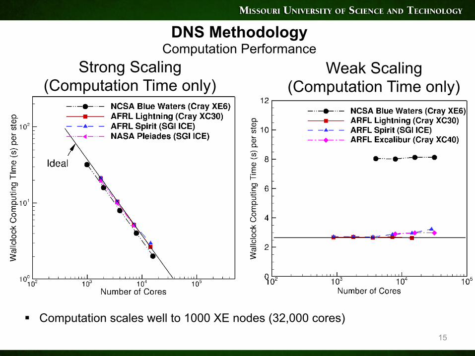
DNS Methodology Computation Performance

Strong Scaling (Computation Time only)

Weak Scaling (Computation Time only)

§  Computation scales well to 1000 XE nodes (32,000 cores)

16

DNS Methodology IO Performance

Parallel IO: parallel HDF5 Pencil size: 16x16x500 Data Size/core: 7.6 MB on each core Stripe count = 4

Weak Scaling (I/O Time only)

§  IO Scalability deteriorate at 1,000 XE nodes (32,000 cores)

17

Results of Domain Science Multivariate statistics and structure of global pressure field

induced by high-speed turbulent BLs

(a)Wall (b)zref/δ = 0.15

(c)zref/δ = 0.73 (d)Freestream

( ) ( ) 2/122/1

2 ),,,('),,,('

),,,('),,,('

),,,(

tzyyxxptzyxp

tzyyxxptzyxp

zzyxC

ref

ref

refpp

Δ+Δ+

Δ+Δ+

=ΔΔ

M∞ = 5.86, Tw/Tr = 0.25 Reτ = 450 (Zhang et al. JFM 2017)

Spatial Pressure Structure

Gray contours: density gradient Color contours: magnitude of vorticity

Freestream Acoustic Radiation M∞ = 5.86, Tw/Tr = 0.25, Reτ = 450 (Zhang et al. JFM 2017)

Spatial-Temporal Correlation of Pressure Structures

20

Space-time correlation Cpp(Δx, 0, 0, Δt)

9.3. CORRELATION COEFFICIENTS 259

Figure 9.16: Variation of the longitudinal space-time correlation with increasingtime delay τ . From Tennekes & Lumley.

Figure 9.17: Correlation measurements showing the decay of maximum correlationlevel with increasing time delay τ .

9.3.3 Space-time correlations

These correlations are taken at different positions and different instants, andthey can be useful for indicating the evolution of certain features, such as thecoherence length of an “average large-scale motion.” Figure 9.16 illustrateshow the space-time correlation changes with increasing time delay τ . Fig-ure 9.18 shows the connection with an “equivalent” space correlation usingTaylor’s hypothesis.

Another example is given in figure 9.18. Here two hot wires were used tomeasure the space-time correlation curves for the streamwise component ofthe velocity and a separation in the streamwise direction (that is, R11). Theindividual correlation curves are shown, as well as a curve drawn to connectthe maxima. This curve gives some measure of the rate at which the largescale motions change their character. Note that the curve decays much morequickly in a subsonic boundary layer than it does in the supersonic case.

Figure 9.19 shows some examples of space time correlations for the stream-

pressure structure at t = 0, x = 0

pressure structure at t = Δt, x = UcΔt

(i)  “frozen propagation” (Taylor’s hypothesis)

(ii) “non-frozen propagation” (Propagation + Evolution)

(correlation decays)

Cpp(Δx, 0, 0) with zero time delay

Cpp(Δx, 0, 0) with time delay Δt

UcΔt

Propagation of Pressure Structures M∞ = 5.86, Tw/Tr = 0.25, Reτ = 450 (Zhang et al. JFM 2017)

21

Uc ≡ −(∂p /∂t)(∂p /∂x)(∂p /∂x)2

Propagation speed defined by finding a value of Uc that minimizes the difference between the real time evolution of p(x, t) and a frozen wave p(x – Uct) (Del Alamo & Jimenez, JFM 2009)

•  Within most of the boundary layer, Uc ≈ <u> (similar to incompressible flow results by Kim & Hussain 1993)

•  In the free stream, Uc departs from Taylor’s hypothesis and is significantly lower than the local mean velocity <u>

Evolution of Pressure Structures M∞ = 5.86, Tw/Tr = 0.25, Reτ = 450 (Zhang et al. JFM 2017)

22

9.3. CORRELATION COEFFICIENTS 259

Figure 9.16: Variation of the longitudinal space-time correlation with increasingtime delay τ . From Tennekes & Lumley.

Figure 9.17: Correlation measurements showing the decay of maximum correlationlevel with increasing time delay τ .

9.3.3 Space-time correlations

These correlations are taken at different positions and different instants, andthey can be useful for indicating the evolution of certain features, such as thecoherence length of an “average large-scale motion.” Figure 9.16 illustrateshow the space-time correlation changes with increasing time delay τ . Fig-ure 9.18 shows the connection with an “equivalent” space correlation usingTaylor’s hypothesis.

Another example is given in figure 9.18. Here two hot wires were used tomeasure the space-time correlation curves for the streamwise component ofthe velocity and a separation in the streamwise direction (that is, R11). Theindividual correlation curves are shown, as well as a curve drawn to connectthe maxima. This curve gives some measure of the rate at which the largescale motions change their character. Note that the curve decays much morequickly in a subsonic boundary layer than it does in the supersonic case.

Figure 9.19 shows some examples of space time correlations for the stream-

Cpp(Δx, 0, 0, Δt)

Δt=0

Δx

Curve of maximum correlation (Cpp)max

(Cpp)max measures the rate of evolution and defines the Lagrangian decorrelation length of coherent pressure structures or wavepackets

23

Sources of Freestream Acoustic Radiation M∞ = 5.86, Tw/Tr = 0.25, Reτ = 450 (Zhang et al. JFM 2017)

Acoustic analogy (Phillips 1960)

Acoustic radiation due to supersonic turbulent boundary layer 187

medium for the left-hand side. Phillips (1960) extended Lighthill’s ideas to treat thenoise radiation problem for supersonic shear flows by accounting for convection withthe mean flow as described below. A more general formulation of the acoustic analogywas presented by Goldstein (2001).

To analyse the generation of sound in a parallel shear flow, Phillips (1960)rearranged the Navier–Stokes equations into a form that, after neglecting the diffusiveterms, can be represented as

⇢D2

Dt2� @

@xia2 @

@xi

�log

✓pp0

◆= �

@ui

@xj

@uj

@xi, (4.1)

where p0 is a convenient reference pressure, D/Dt is the substantial derivative basedon mean flow velocity, and � is the specific heat ratio.

The terms on the left-hand side of (4.1) are those of a wave equation in a mediummoving with the local mean velocity of the flow. It is evident that the effects ofconvection and variation of local speed of sound have been included on the left-handside, since both effects are an integral part of acoustic propagation in high-speed flows.The term on the right-hand side, which is quadratic in the total flow velocity, is theacoustic source term. By decomposing the total velocity into a mean plus a fluctuatingcomponent, the acoustic source term can be further represented as those that are bothlinear and quadratic in the fluctuating velocity components:

@ui

@xj

@uj

@xi= 2

@U@z

@w0

@x+ @u0

i

@xj

@u0j

@xi. (4.2)

The linear source term represents the generation of pressure fluctuations by theinteraction of turbulence with the mean shear (where only the dominant linear terminvolving the mean flow shear @U/@z is shown for brevity), while the nonlinear sourceterm represents the generation of pressure fluctuations by the interaction of turbulencewith itself. In the context of incompressible flows, the mean shear term is known asthe rapid source term, whereas the nonlinear self-interaction term involving turbulentfluctuations is known as the slow pressure source (Kim 1989). In the following, wewill investigate the origin of free-stream noise by investigating the characteristics ofthe acoustic source terms within the boundary layer.

Figure 17(a) plots the r.m.s. value of the acoustic source term as well as itslinear and nonlinear components as functions of z across the near-wall portion of theboundary layer. It is shown that the total source term peaks at z+ ⇡ 20, i.e. withinthe buffer-layer region of the turbulent boundary layer. The nonlinear source term isdominant over the linear source term throughout the boundary layer and constitutesalmost all of the total source. Further breakdown of the nonlinear term into its sixconstituent terms shows that (@v0/@z)(@w0/@y) has the largest r.m.s. value over mostof the boundary layer (figure 17b) and peaks at approximately z+ = 20. Since theturbulent structures at this height are dominated by near-wall streamwise structures,the latter structures may well play an important role in sound generation, at least atMach 2.5. A similar distribution of source terms as well as the dominance of thenonlinear components have been observed by Kim (1989) in the study of turbulentpressure fluctuations for incompressible channel flows (see figures 18–20).

We note that the solution to the acoustic analogy (4.1) is given by the convolutionof the source terms with the Green’s function of this equation, which may beviewed as the local efficiency of the conversion of hydrodynamic source terms into

Nonlinear source Linear source

Acoustic radiation due to supersonic turbulent boundary layer 187

medium for the left-hand side. Phillips (1960) extended Lighthill’s ideas to treat thenoise radiation problem for supersonic shear flows by accounting for convection withthe mean flow as described below. A more general formulation of the acoustic analogywas presented by Goldstein (2001).

To analyse the generation of sound in a parallel shear flow, Phillips (1960)rearranged the Navier–Stokes equations into a form that, after neglecting the diffusiveterms, can be represented as

⇢D2

Dt2� @

@xia2 @

@xi

�log

✓pp0

◆= �

@ui

@xj

@uj

@xi, (4.1)

where p0 is a convenient reference pressure, D/Dt is the substantial derivative basedon mean flow velocity, and � is the specific heat ratio.

The terms on the left-hand side of (4.1) are those of a wave equation in a mediummoving with the local mean velocity of the flow. It is evident that the effects ofconvection and variation of local speed of sound have been included on the left-handside, since both effects are an integral part of acoustic propagation in high-speed flows.The term on the right-hand side, which is quadratic in the total flow velocity, is theacoustic source term. By decomposing the total velocity into a mean plus a fluctuatingcomponent, the acoustic source term can be further represented as those that are bothlinear and quadratic in the fluctuating velocity components:

@ui

@xj

@uj

@xi= 2

@U@z

@w0

@x+ @u0

i

@xj

@u0j

@xi. (4.2)

The linear source term represents the generation of pressure fluctuations by theinteraction of turbulence with the mean shear (where only the dominant linear terminvolving the mean flow shear @U/@z is shown for brevity), while the nonlinear sourceterm represents the generation of pressure fluctuations by the interaction of turbulencewith itself. In the context of incompressible flows, the mean shear term is known asthe rapid source term, whereas the nonlinear self-interaction term involving turbulentfluctuations is known as the slow pressure source (Kim 1989). In the following, wewill investigate the origin of free-stream noise by investigating the characteristics ofthe acoustic source terms within the boundary layer.

Figure 17(a) plots the r.m.s. value of the acoustic source term as well as itslinear and nonlinear components as functions of z across the near-wall portion of theboundary layer. It is shown that the total source term peaks at z+ ⇡ 20, i.e. withinthe buffer-layer region of the turbulent boundary layer. The nonlinear source term isdominant over the linear source term throughout the boundary layer and constitutesalmost all of the total source. Further breakdown of the nonlinear term into its sixconstituent terms shows that (@v0/@z)(@w0/@y) has the largest r.m.s. value over mostof the boundary layer (figure 17b) and peaks at approximately z+ = 20. Since theturbulent structures at this height are dominated by near-wall streamwise structures,the latter structures may well play an important role in sound generation, at least atMach 2.5. A similar distribution of source terms as well as the dominance of thenonlinear components have been observed by Kim (1989) in the study of turbulentpressure fluctuations for incompressible channel flows (see figures 18–20).

We note that the solution to the acoustic analogy (4.1) is given by the convolutionof the source terms with the Green’s function of this equation, which may beviewed as the local efficiency of the conversion of hydrodynamic source terms into

Acoustic source term Wave Operator

•  Nonlinear source (NLS) dominates over linear source (LS) •  Total acoustic source term peaks in the buffer layer (z+

pk ≈ 20)

Summary §  Cutting-edge computational power of the Blue Waters is used to generate a DNS

database of high-speed turbulent boundary layers •  M∞ = 2.5 – 14 •  Tw/Tr = 0.18 - 1.0 •  Reτ ≈ 400 – 2000

§  DNS database is used to study the boundary-layer-induced global pressure field

•  pressure statistics and structures

•  freestream acoustic radiation

§  DNS code is being modernized on the Blue Waters to enable petascale simulations at higher Reynolds numbers

•  Software profiling

•  Parallel I/O

•  Hybrid MPI-OpenMP

24

Future Work

§  Conduct DNS of supersonic turbulent boundary layers at Reτ ≈ 2000 •  investigate statistical and spectral scaling of the global pressure field •  dependence of the induced pressure field on Reynolds number

§  DNS code modernization •  hybrid MPI-OpenMP parallel structure •  An additional dimension of domain decomposition

25

MPI-OpenMP Hybridization

Computational Domain

MPI ranks decomposeinto pencils (2D decomposition)

Pencil

Thread level pencils, here called windows

MPI rank

Thread

Current work

Acknowledgment

•  Dr. Meelan Choudhari at NASA Langley Research Center –  for collaboration

•  Funding Support –  AFOSR (Award No. FA9550-14-1-0170)

–  NASA (Cooperative Agreement No. NNL09AA00A)

•  Computing resources

–  NCSA through NSF PRAC (Award No. ACI-1640865)

–  DoD High Performance Computing Modernization Program

–  NASA Advanced Supercomputing Division

27

Publications •  J. Huang and L. Duan, “Turbulent Inflow Generation for Direct Simulations of Hypersonic

Turbulent Boundary Layers and Their Freestream Acoustic Radiation”, AIAA Paper 2016-3639, 46th AIAA Fluid Dynamics Conference, Washington, DC, June, 2016. http://arc.aiaa.org/doi/abs/10.2514/6.2016-3639

•  C. Zhang and L. Duan, “Multivariate Statistics Analysis of the Pressure Field Induced by High-Speed Turbulent Boundary Layers”, AIAA Paper 2016-3090, 46th AIAA Fluid Dynamics Conference, Washington, DC, June, 2016.http://arc.aiaa.org/doi/abs/10.2514/6.2016-3190

•  L. Duan, M. M. Choudhari and C. Zhang, “Pressure fluctuations induced by a hypersonic turbulent boundary layer”. Journal of Fluid Mechanics, 2016, 804, 578-607.

•  C. Zhang, L. Duan and M. M. Choudhari , “Effect of wall cooling on boundary-layer-induced pressure fluctuations at Mach 6”, Journal of Fluid Mechanics, in press, 2017.

Reference •  William K. Blake, Mechanics of Flow-Induced Sound and Vibration V2, 1986 •  Arndt, R. E. (2002). Cavitation in vortical flows. Annual Review of Fluid

Mechanics, 34(1), 143-175. •  S. B. Pope, Turbulent Flows, Cambridge University Press, Aug 10, 2000 •  Laufer, J. (1964). Some statistical properties of the pressure field radiated by a

turbulent boundary layer. The Physics of Fluids, 7(8), 1191-1197. •  Beresh, S. J., Henfling, J. F., Spillers, R. W., & Pruett, B. O. (2011). Fluctuating

wall pressures measured beneath a supersonic turbulent boundary layer. Physics of Fluids, 23(7), 075110.

•  Pirozzoli, S. (2010). Generalized conservative approximations of split convective derivative operators. Journal of Computational Physics, 229(19), 7180-7190.

•  Martín, M. P., Taylor, E. M., Wu, M., & Weirs, V. G. (2006). A bandwidth-optimized WENO scheme for the effective direct numerical simulation of compressible turbulence. Journal of Computational Physics, 220(1), 270-289.

•  Jiang, G. S., & Shu, C. W. (1996). Efficient implementation of weighted ENO schemes. Journal of computational physics, 126(1), 202-228.

29

•  Taylor, E. M., Wu, M., & Martín, M. P. (2007). Optimization of nonlinear error for weighted essentially non-oscillatory methods in direct numerical simulations of compressible turbulence. Journal of Computational Physics, 223(1), 384-397.

•  Ducros, F., Laporte, F., Souleres, T., Guinot, V., Moinat, P., & Caruelle, B. (2000). High-order fluxes for conservative skew-symmetric-like schemes in structured meshes: application to compressible flows. Journal of Computational Physics, 161(1), 114-139.

•  Xu, S., & Martin, M. P. (2004). Assessment of inflow boundary conditions for compressible turbulent boundary layers. Physics of Fluids, 16(7), 2623-2639.

•  Del Álamo, J. C., & Jiménez, J. (2009). Estimation of turbulent convection velocities and corrections to Taylor's approximation. Journal of Fluid Mechanics, 640, 5-26.

•  Kim, J., & Hussain, F. (1993). Propagation velocity of perturbations in turbulent channel flow. Physics of Fluids A: Fluid Dynamics, 5(3), 695-706.

•  Phillips, O. M. (1960). On the generation of sound by supersonic turbulent shear layers. Journal of Fluid Mechanics, 9(01), 1-28.

30

Questions?

31

Backup

32