Copyright ©1997, American Institute of Aeronautics and Astronautics, Inc.

AIAA Meeting Papers on Disc, January 1997A9715767, F49620-94-1-0019, F49620-95-1-0405, AIAA Paper 97-0755

Direct numerical simulation of hypersonic boundary-layer transition over bluntleading edges. I - A new numerical method and validation

Xiaolin ZhongCalifornia Univ., Los Angeles

AIAA, Aerospace Sciences Meeting & Exhibit, 35th, Reno, NV, Jan. 6-9, 1997

This paper presents and tests a new high-order upwind finite difference shock fitting method for the direct simulations ofhypersonic flows with strong bow shocks. There are three main aspects of the new method: a simple unsteady shock fittingformulation, new upwind high-order finite difference schemes for spatial discretization, and new third-order semi-implicitRunge-Kutta schemes for temporal discretization. The results of accuracy tests of the new fifth-order shock-fitting methodare presented for four test cases: 1D wave equation, 2D direct numerical simulation (DNS) of stability of supersonic Couetteflow, steady viscous hypersonic flow over a circular cylinder, and the DNS of receptivity to freestream acoustic disturbancesfor hypersonic boundary layers over a parabola. (Author)

Page 1

Direct Numerical Simulation of Hypersonic Boundary-Layer Transition Over BluntLeading Edges, Part I: A New Numerical Method and Validation

Xiaolin Zhong *University of California, Los Angeles, California 90095

Abstract

Direct numerical simulation (DNS) of the stabilityand transition of hypersonic boundary layers over bluntleading edges requires high-order accurate numericalmethods to resolve a wide range of time and lengthscales. In addition, numerical methods for such simu-lation need to resolve unsteady bow shock motion andshock/disturbance interaction accurately. This paperpresents and tests a new high-order upwind finite dif-ference shock fitting method for the direct simulationsof hypersonic flows with strong bow shocks. Thereare three main aspects of the new method: a simpleunsteady shock fitting formulation, new upwind high-order finite difference schemes for spatial discretiza-tion, and new third-order semi-implicit Runge-Kuttaschemes for temporal discretization. The results of ac-curacy tests of the new fifth-order shock-fitting methodare presented in this paper for four test cases: 1-Dwave equation, 2-D DNS of stability of supersonic Cou-ette flow, steady viscous hypersonic flow over a cir-cular cylinder, and finally, the DNS of receptivity tofreestream acoustic disturbances for hypersonic bound-ary layers over a parabola.

Introduction

The prediction of laminar-turbulent transition in hy-personic boundary layers is a critical part of the aero-dynamic design and control of advanced hypersonicvehicles '1>2'L Recently, direct numerical simulation hasbecome a powerful tool in the study of fundamentalflow physics of the stability and transition of boundarylayers f3'4^. The direct numerical simulation approachstudies the transitional boundary layers ̂ by numer-ically solving the time-dependent three-dimensionalNavier-Stokes equations for the temporally or spatiallyevolving instability waves. Such simulation requiresthat all relevant flow time and length scales are re-solved by the numerical solutions using highly accuratenumerical methods.

'Assistant Professor, Mechanical and Aerospace EngineeringDepartment, Member AIAA.

Copyright ©1997 by American Institute of Aeronautics and As-tronautics, Inc. All rights reserved.

Most DNS work on boundary layer transition arefor incompressible flows l5"14!. The DNS of compress-ible boundary layer transition has occurred only in thelast few years. Erlebacher et al. I15'16' studied the sec-ondary instability mechanism of compressible bound-ary layers over a flat plate by temporal and spatial di-rect numerical simulations. Thumm et al. t17-', Faselet al.[18], and Eibler et al.[19'201 performed spatialDNS of the oblique breakdown of transition in a su-personic boundary layer over a flat plate. Adams andKleiser P1'22! studied the subharmonic transition pro-cess of a flat-plate at a freestream Mach number of 4.5by temporal direct numerical simulation. This workwas extended to spatial DNS of a flat-plate boundarylayer of Mach 1.6 to 4.5 by Guo et al. ^3' in the sameresearch group. Pruett and Zang I-24-' conducted tem-poral DNS studies of laminar breakdown in high-speedaxisymmetric boundary layers over a hollow cylinderand a sharp cone. Pruett et al. I25"27) then performedspatial simulations for supersonic boundary layers overflat plates and sharp cones. These DNS studies of com-pressible boundary layers show that the DNS of high-speed boundary transition is feasible on existing com-puters using efficient and accurate numerical methods.So far, DNS studies of compressible boundary layershave been limited to perfect gas flows over simple flatbody surfaces without the presence of shock waves.

This paper is concerned with numerical methodsfor the DNS of stability and transition of hypersonicboundary layers behind blunt bodies (Fig. 1). For theDNS of such flows, it is difficult to apply the existingmethods due to the lack of efficient semi-implicit nu-merical methods for compressible viscous flows, pres-ence of shock waves, and the stiffness of the equationsin reacting hypersonic flows. This paper presents anew high-order (fifth and sixth order) upwind finitedifference shock fitting method for the direct simula-tion of hypersonic flows with a strong bow shock andwith stiff source terms. There are three main aspectsof the new method for hypersonic flow DNS: a newshock fitting formulation, new upwind high-order fi-nite difference schemes, and third-order semi-implicitRunge-Kutta schemes recently derived t28'.

First, a shock fitting formulation, which is verysimple for the high-order discretization in three-

dimensional shock fitting calculations with unsteadyshock motion, is presented in this paper. The use ofshock fitting method makes it possible to use high-order linear schemes for spatial discretization of theflow equations behind the bow shock. Hussaini, Ko-priva, Salas, and Zang '29' used the shock fitting spec-tral method to simulate shock/turbulent interaction.Recently, Cai '30^ used a shock fitting method to com-pute two-dimensional detonation waves. This paperpresents a simple formulation for shock fitting calcu-lation of three-dimensional unsteady hypersonic flows.The current formulation is simple because the pertur-bation relation across the shock is consistent with con-servative flux and its Jacobian used in the conservationequations. As a result, high-order schemes can be ap-plied to the shock fitting calculations easily.

Second, new upwind compact and explicit high-orderfinite difference schemes derived in a recent paper ̂are used in computing inviscid fluxes. Most finite dif-ference methods used in direct numerical simulationshave been central difference schemes I26-32-33] contain-ing only phase errors without any numerical dissipationerrors. However, high-order central schemes are of-ten not robust enough for convection dominated prob-lems. Extra filtering procedures, which are equivalentto adding numerical dissipation, are often required tocontrol the aliasing errors and to stabilize the com-putations. In addition, central difference schemes offourth order or higher are often unstable when they arecoupled with high-order boundary schemes using sim-ple one-sided finite difference approximations i26>34>35J.Boundary closure schemes, which are needed because ofwide grid stencils of high-order inner schemes, often de-termine the overall accuracy of the computations usinghigh-order inner schemes. For a global scheme of p-ihorder ' ', the boundary schemes have to be at least p-1-th order. Carpenter, Gottlieb, and Abarbanel [34'35]

showed that for a sixth-order inner central compactscheme, only a third-order boundary scheme can beused without introducing instability. The resulting sta-ble 3,4-6-4,3 compact scheme, which denotes a sixth-order inner scheme with third and fourth order bound-ary schemes at the first and second boundary pointsrespectively <-35\ is fourth order globally accurate eventhough the inner scheme is sixth-order accurate. Onthe other hand, Rai and Moin '•37^ showed that modernupwind schemes are very robust even when they aremade high-order accurate. Ref. [37] used a spatiallyfifth-order upwind-bias explicit finite difference schemefor solving the Navier-Stokes equations. The implicitnumerical dissipation in the upwind-bias schemes isenough to control the aliasing errors. In recent years,many other upwind high-order schemes have also beendeveloped I38"41! for the direct numerical simulation oftransitional and turbulent boundary layers or other

flows.

The upwind schemes presented in [31] use centralgrid stencils with built-in implicit numerical dissipa-tion, similar to the fifth-order explicit upwind schemeof Zingg et al. ̂ and the 4th-order compact upwindschemes of Adams and Shariff'41-'. The current up-wind schemes, which include both upwind compact andexplicit schemes, are more general and systematic inderivation and analysis. The orders of accuracy of thecurrent upwind schemes are one-order lower than themaximum orders the central stencils can achieve. Eachupwind scheme contains an adjustable coefficient in theleading dissipative truncation term. The free parame-ter is chosen so that the upwind schemes do not haveexcessive numerical dissipation in the simulations andthe inner schemes are stable when they are coupledwith high-order numerical boundary schemes. The dis-sipation errors of the schemes are set to be smaller orcomparable to the phase errors for well resolved lowwavenumber modes and to damp out unresolved higherwavenumber modes. For the stability of the high-orderinner schemes with boundary schemes, asymptotic sta-bility of the schemes is analyzed by computing theeigenvalue spectrums of spatial approximations withboundary schemes. It is found that the high-order up-wind schemes help to stabilize the overall schemes whenthey are coupled with high-order boundary closures.

Third, the time advancement of the governingequations with stiff viscous terms in the boundarylayer or thermo-chemical nonequilibrium source termsis solved by third-order semi-implicit Runge-Kuttaschemes I42'43!. The third-order semi-implicit Runge-Kutta schemes are able to compute stiff reactive flowequations with third-order temporal accuracy, andThey are unconditionally stable for the stiff terms whenthe non-stiff terms satisfy explicit stability conditionsfor the Runge-Kutta schemes.

Governing Equations

Though real gas effects become important as gastemperature increases ̂ for hypersonic flow behinda strong bow shock, perfect gas assumption is used inthis paper. The method can be extended to nonequi-librium real-gas flow if necessary. The governing equa-tions are the unsteady three-dimensional Navier-Stokesequations:

dt= (1)

where 77, £, r) as follows

U — {Pi P u l j PU2> PU3> e]

Fj = =

+ P)

= pRTp(cvT+£

dT

(2)

(3)

(4)

(5)(6)

(8)

l_dU_ dE' dF' dG'

dE'v , dF'v .

where

E'

F'

G'

F'v

G'v

l + rjnJ2 = lL (10)OT J

J

J

J+ Fy lt]y +

J

+ FylCy +

J

(11)

(12)

(13)

(14)

(15)

(16)

A shock fitting method is used to solve unsteadythree-dimensional viscous hypersonic flow over a wedgeshown in Figure 2. The general curvilinear three-dimensional coordinates (£, 77, f, T) are used along thebody fitted grid lines (Fig. 2). Shock fitting methodsare used to treat the bow shock as a computationalboundary. The transient movement of the shock andits interaction with disturbance waves are solved aspart of the solutions. Therefore, the grid surface of77 = constant is unsteady due to the shock movement,but the grid surfaces of £ = constant and £ = constantare fixed plane surfaces during the calculations. In par-ticular, the £ = constant surfaces are generated suchthat they are normal to the wall surface. Therefore,only the rj = constant grid lines change when the bowshock moves.

The transformation relations for the current grid sys-tems are

where J is the Jacobian of the coordinate transforma-tion, and £,, £„, &, r)x, riy, r)z, r)t, Cr, Cy, and £, arethe grid transformation metrics, which are computedas functions of the body shape, the grid-point distri-bution along the grid lines, the wall-normal distanceH(£>G>T) between the shock and the wall along the77 grid lines (see Fig. 2), and the time derivative HT.These metrics functions are functions of time throughH and HT.

The governing equations are discretized in the uni-form computational space. In the equations, the trans-formed inviscid fluxes E', F', and G' are standardflux terms with known eigenvalues and eigenvectors.The transport flux terms E'v, F^, and G'v contain first-order spatial derivatives of velocity and temperature.These derivatives in the Cartesian coordinates (x, y, z)are transformed into the computational coordinates(£i ^iC) using a chain rule for spatial discretization.

(9)

T=t t-T

A Simple Shock Fitting Formulation

The shock fitting method treats the bow shock as acomputational boundary at 77 = f?max as

where & = 0 and £t = 0 because the ^ and C grid linesare fixed when the shock boundary moves.

r)(x, y, z, t) = r;max = constant (17)

In the numerical simulations, the governing equation The flow variables behind the shock are determined by(1) are transformed into the computational domain (4, the Rankine-Hugoniot relation across the shock and a

characteristic compatibility equation from behind theshock. As shown in Fig. 2, the position and veloc-ity of the shock front are functions of H(£, £, T) andHT(£,£,T), which are solved as unknown variables us-ing high-order finite difference methods. A simple for-mulation for the governing equations for the shockmovement is derived in the section. The method issimilar to that used by Cai [30], but is simplier in ob-taining the shock equations by using the same metricsand flux Jacobian as those used in discretization of in-terior governing equations.

The normal vector of the shock front is

P, = Po\l +

es.iP,{

(7-

(itn, -

(25)

(26)

(27)(28)

where M«o is the normal component of the incomingMach number relative to the shock based on the speedof sound, u is the velocity vector, Ut is the tangentialvelocity vector, «„ is the normal velocity component.The definitions for these variables are

_ (18)

and the velocity of the shock front in the direction ofu is

rjt (19)

The flow variables across the shock are governed bythe Rankine-Hugonoit conditions:

E" — c"1s ~ C0 (20)

where the subscript s represents the variable immedi-ately behind the shock and subscript 0 represents thevariable on the free stream side of the shock surface.The flux F', which is the flux in the computationalspace along the 77 grids line, is given by Eq. (12) as

F' =

J

where

F = F3k

(21)

(22)

(23)

The Rankine-Hugoniot relations lead to jump condi-tions for flow variables behind the shock as functionsof Uo and the grid velocity vn, i.e.,

(24)P, = Po 1 +

COu • nu — wnn

(29)

(30)(31)

In order to compute the flow variable behind the shockusing the shock jump conditions above, the velocityof the shock front vn is needed. The shock normalvelocity is computed by a characteristic relation behindthe shock.

In order to solve the shock movement, a character-istic compatibility equation at the grid point imme-diately behind the shock is needed. It is found thatthe shock fitting computations and the shock geome-try transformation relations are greatly simplified if wederive the characteristic compatibility equation in theconservation-law form, which can de derived directlyfrom Eq. (1) in the direction along the rj coordinates.Specifically, the interior equation (1) in the compu-tational domain at the point immediately behind theshock front can be written as:

J dr+dF"drj

W_J

9E' dG'

8r, dr J (32)

where the equation is evaluated at point s behind theshock. In the equations, the Jacobian matrix, B'a —(dF'ldU)a, has the following eigenvalues:

J|Vf?|

(un - (un -vn)s,

Un -Vn -C)s, (33)

The corresponding left eigenvectors are

la, 12, • • - , IN-I, IN (34)

where N is the number of independent variables in theequations. Specifically, the left eigenvector IN is '45-'

N

where

c2

-(|cn« - f u)-(!«>» - f «)-(§«»» - f «0

£2

"^K = 7 — !

(35)

(36)

(37)

By definition, the left eigenvector behind the shock sat-isfies:

IN-5' = (38)

where the flux Jacobian

B' = aF7

817(44)

is the Jacobian of the 77 direction flux defined in theconservation equations (10), and

dr_

dr

dr dr dr

dr (46)

These time derivatives of the grid metrics can be de-rived by the same methods as those used in discretiza-tion of the interior equations.

Finally, the equation for the shock velocity can beobtained by multiplying both sides of Eq. (43) by INand using the relation of (38), i.e.,

The characteristic field approaching the shock frombehind corresponds to the eigenvalue of *-j^(wn — vn +c)a. The compatibility relation for this characteristicfield can be obtained by multiplying Eq. (32) by IN,

du fW dE1 dF' 8G'~ N ' V J d£ drj 9C

On the other hand, the shock jump condition (20)can be rewritten as

'] = (Fs-F0)-a+(US -U0)b = 0 (40)

where

-1dr !N • (U, - U0)]

(47)

where the term IN • ̂ - is computed using the char-acteristic relation (39), in which the spatial derivativesare discretized together with the discretization of theinterior points for the Eq. (10) using the same schemesat the interior algorithm applied to boundary behindthe shock. In the equation above, J£ and |̂ can beexpressed as function of H and HT as follows

p = di(€, C, H, Hr) + d2(e, C, H, HT) f. (48)fla

= d(t,C,H,Hr) (49)

a = .

* = (?).-

. (41)

(42)

Taking derivative of Eq. (40) with respective to r inthe computational space leads to

, 8U. dU0

(43)

The coefficients, di, d^, and vector g are functions ofgrid metrics.

Therefore, the equation for the shock accelerationcan be obtained from Eqs. (48) to (49) in the followingform:

dHTdr C,

O) -Q— (50)

dJL6r (51) dimensional linear wave equation:

The two equations above describe the shock normalvelocity and shock shape, and they can be integratedin time simultaneously with the interior flow variablesusing Runge-Kutta methods. After the values ofH andHT are determined, the flow variables behind the shockcan be computed by the jump conditions across theshock using Eqs. (24) to (28). The grids and metricsare modified according to the new values of H and Hr.

The current formulation is simple because the gov-erning equations for the shock movement are derivedusing conservative variable and flux Jacobian in Eq.(43) using the relation (38). The same discretizationof the interior governing equations is used to evaluateIN • ( ^ f ) s a^ grid points immediately behind the shock.In addition, all geometric definitions of the shock frontare the same as the grid metrics used in the interiorequation transformation, which are stored in the com-puter. In doing so, the current approach avoids compli-cation of using the non-conservation variables and lo-cally defined geometric parameters for the shock frontin deriving the time derivatives of the shock jump con-dition.

High-Order Upwind Schemes forSpatial Discretization

The governing equation (10) is discretized in thecomputational domain (£, r), C, T] using the methodof lines. Because there is no shock in the computa-tional domain, high-order finite difference methods areused for spatial discretization of the equations, wherethe inviscid and viscous flux terms are discretized us-ing different methods: central difference schemes forthe viscous flux terms and upwind schemes for the in-viscid flux terms.

In Ref. [31], a family of finite-difference upwindschemes of third, fifth, and seventh orders have beenderived for the direct numerical simulations of hyper-sonic boundary layers. Either compact or non-compact(explicit) schemes can be used. Each upwind schemeuses a central stencil with a free damping parametera, which is chosen such that the inner scheme is stablewhen it is coupled with high-order numerical bound-ary schemes and the dissipation errors are smaller orcomparable to phase errors. These high-order upwindschemes are used for the spatial discretization in theshock-fitting algorithm.

The upwind schemes are described using the one-

du du= 0 a<x<b (52)

where c > 0. The downwind algorithm for negative ccan be derived similarly.

The linear wave equation (52) is solved by themethod of lines, where the spatial derivative, du/dx,is first discretized in space while keeping the tempo-ral derivative hi the equations. The general finite-difference approximation for du/dx located at i-th gridpoint can be written as I32'41-*

Mo

k=-M+M0+l

= \ £ ai+kui+k (53)

where uniform grids with grid spacing of h are assumed,and u'i+k is the numerical approximation of du/dx lo-cated at (z'+&)-th grid point. On the right hand side ofthe equation, a total of N grid points are used for U{+kwith JVo points bias with respect to the based pointi. A similar grid combination of M and MO is usedfor u'i+k on the left hand side of the equation. In thispaper, a scheme using this grid combination is termedthe N-No-M-Mo scheme, which includes both compactand explicit schemes as its special cases. For example,the schemes are compact finite difference schemes whenM >2, and they are explicit finite difference schemeswhen M — I and MO = 0.

Ref. [31] considered a family of upwind compact andexplicit high-order finite difference methods using cen-tral grid stencils, i.e.,

N = 27VO + 1 (54)M = 2M0 + 1 (55)

The coefficients 0,-+* and 6,-+^ of the upwind schemesare determined such that the order of the schemes isone order lower than the maximum achievable order forthe central stencil, i.e, the orders of the upwind schemesare always odd integers of p = 2(No + MQ) — I . As aresult, there is a free parameter a in the coefficientsa,-+fc and 6,-+^. The free parameter is set to be thecoefficient of the leading truncation term which is a

derivative even order, i.e.,

Mo n

E »««»«4k=-M0 k=-No

(56)

160T" •40u,-+i + -ru,-+j (58)

Fifth-Order Upwind Explicit Schemes:

where p = 2(A^0 + Mo) — 1, and a is the free parameter.All schemes with nonzero a are p-th order accurate,and they are central schemes of (p+l)-th order whena = 0. The choice of a is not unique, and it has ef-fects mainly on the magnitudes of numerical dissipa-tion. The specific value of a for an upwind scheme ischosen to be large enough to stabilize the high-orderupwind inner scheme when it is coupled with stableboundary closure schemes, and to be small enough sothat the dissipation errors are comparable to the dis-persion errors of the inner scheme.

The detailed expressions of the upwind compact andexplicit upwind schemes of fifth and seventh orders aregiven below. Ref. [31] chose a set of "recommended"values of a based on the accuracy and stability analysis.Since compact schemes with large M involve costly so-lutions of linear equations in computing derivatives, weare mainly interested in three-point compact schemes(M = 3). The third-order compact and explicit up-winds schemes and the upwind seventh-order five-pointcompact schemes with a 5-2-5-2 stencil are given in [31].

Fifth-Order Upwind Compact Schemes:

"„• = —— ai+k ui+k*=-3

(59)

where

= ±45 + f c0-fa 6,- = 60

These 7-3-1-0 schemes are fifth-order upwind schemewhen a < 0, and they are sixth-order central schemewhen a = 0. The recommended value for a is a = —6,and the corresponding fifth-order upwind explicit innerscheme is

105

— ui+i - 6«i+2 + 2 (60)

where

(57) It is noted that the fifth-order upwind bias scheme ofRai and Moin ' 'is a special case of the current 5th-order upwind schemes corresponding to a = —12 andOi+3 = 0. The stencil of the scheme becomes upwind-bias (6-2-1-0). The recommended upwind schemeabove has less numerical dissipation because of smaller

Ui = 0 — 15a

_"~1 I s3, 5.

= 60= 20 -5a

Seventh-Order Upwind Compact Schemes:

These 5-2-3-1 schemes are fifth-order upwind compactschemes when a < 0, and they reduce to the sixth-order central compact scheme when a = 0. The rec-ommended value for a is a — — 1, which corresponds tothe following fifth-order upwind compact inner scheme:

(61)

where

1

— - -+•3-ia

= U-T §c_ 375

= f-|a= 60

65

a,-_2 = -3->&,-_! = a

These 7-3-3-1 schemes are seventh-order upwind com-pact schemes when a > 0, and they are eighth-ordercentral compact scheme when a ~ 0. The recom-mended value for a is a = 36, and the correspondingseventh-order upwind compact inner scheme is

T-4

Seventh-Order Upwind Explicit Schemes:

(62)

High-order finite difference schemes require addi-tional numerical boundary schemes at grid points nearthe boundaries of the computational domain. For ap-ih order interior scheme, the accuracy of boundaryschemes can be (p— l)-th order accurate without reduc-ing the global accuracy of the interior scheme. For ex-ample, for the fifth-order inner upwind compact schemegiven by Eq. (58), two boundary schemes are needed atgrid point at i = 0, 1, and i = N — 1, N. It is desirablethat the boundary schemes are at least fourth-order sothat overall schemes are fifth-order accurate. Both one-sided compact and explicit finite difference schemes canbe used as numerical boundary schemes. The expres-sions of the boundary schemes of up to sixth order canbe found in [31]. The orders of accuracies for stableoverall schemes when they are coupled with high-orderinterior schemes were analyzed in [31] and are summer-ized in Table 3, where the notation of 3,4-6-4,3 denotedby Carpenter et al. as a sixth-order inner scheme withthird and fourth order boundary schemes at the firstand second boundary points respectively ^35\

Discretization of Inviscid Flux Vectors

«• =

where

a 7(du*\ ,~ ~ (63)

For the inviscid flux vector in the governing equa-tion (10), the flux Jacobians contains both positive andnegative eigenvalues in general. In this paper, a simplelocal Lax-Friedrichs scheme is used to split the inviscidflux vectors into positive and negative wave fields. Forexamplcj the flux term B' in Eq. (10) can be split intotwo terms of pure positive and negative eigenvalues asfollows

a,-±2a,-±ia,

= ±12 t= ±48 - 2L

hi = 60

These 9-4-1-0 schemes are seventh-order upwind ex-plicit schemes when a > 0, and they are eighth-ordercentral explicit scheme when a = 0. The recommendedvalue for a is a = 36, and the corresponding seventh-order upwind explicit inner scheme is

160/i

15 27

13

15—

9

19yMj-3

tr 21+45ui+1 -

(64)

Ef:

where

(65)

*- • i'(66)

(67)

(68)

where A is chosen to be larger than the local maximumeigenvalues of E':

+ w'2 + c (69)

where

Numerical Boundary Schemes (70)

The parameter e is a small positive constant added forthe smoothness of the splitting. The flux E'+ and E'_contain only positive and negative eigenvalues respec-tively. Therefore, in the spatial discretization of Eq.(10), the flux derivatives are split into two terms

= -^2^, ai+k Ui+kk=-2

(£=2,3, • • - , # - 2 ) (74)

BE' _ dE'+~

dE'_(71)

where the first term on the right hand side is discretizedby an upwind high-order finite-difference method andthe second term is discretized by a downwind high-order finite-difference method.

Numerical diffusion is introduced in the Lax-Friedrichs schemes by the splitting of the flux vec-tor. The first-order upwind schemes using the Lax-Friedrichs schemes is very numerically diffusive. Onthe other hand, the inviscid fluxes can also be split ac-cording to their characteristic fields ^6\ which is lessdiffusive. But the characteristic splitting is computa-tionally more expansive and the numerical diffusions ofthe Lax-Friedrichs schemes become much smaller whenfourth or higher order upwind schemes are used for theflow field without shock waves.

Discretization of Transport Flux Vectors

For the compressible Navier-Stokes equations (10)in a conservation-law form, the second-order deriva-tives do not appear explicitly in the equations. Instead,they appear as first-order derivatives in the transportflux vectors in Eq. (4). For such equations, it is eas-ier to discretize the transport terms by applying cen-tral finite-difference operators for the first derivativetwice '•4?J. The approximation of the first-order deriva-tive for computing the viscous terms can be done usingstandard central compact or explicit schemes with one-sided difference approximation For example, the sixth-order central inner schemes (5-3-3-1) and the sixth-order compact boundary schemes are as follows:

15 , _ !_ /215YUjv ~ h \T*

(75)

(76)

where the coefficients for the inner schemes are givenby Eq. (57) with a = 0. The formulas can be writteninto matrix form

BU' = AU (77)

where U = («o> • • • , M/v)T- The derivative of the vis-cous flux in Eq. (10) can be discretized using the samefirst-order operator above. The second-order approx-imation is 6th-order accurate even though the orderat the boundary may be degenerated. Though suchdiscretization leads to a wider grid stencil than us-ing central compact schemes to second-order deriva-tive directly, the eigenvalue analysis shows that suchan approach using the sixth-order central schemes withboundary closures is stable when it is applied to theone-dimensional linear heat equation. Other similarcentral compact and explicit high-order schemes forsecond-order derivatives can be obtained easily.

Semi-Implicit Runge-Kutta Schemes forTemporal Discretization

60«'0 + 300*4 = (-197uo -

+300w2 - + 25«4 - (72)

-50«i 10«s - (73)

The spatial discretization of the governing equationsleads to a system of first-order ordinary differentialequations for the flow variables, and the accelerationsand speeds of the shock fronts. For reacting hypersonicflow simulations, the thermo-chemical source term Wis often stiff in temporal discretization. In Ref. [42,43],Zhong derived three kinds of high-order semi-implicitRunge-Kutta schemes for high-order temporal integra-tion of the governing equations. These schemes addi-tively split the governing equations into stiff and non-stiff terms in the form of

i-i u'i-i + bi u'f + bi+i u'i+i (78)

where u is the vector of discretized flow field variables,f is non-stiff terms resulted from spatial discretiza-tion of the flux terms which can be computed explic-itly, and g is stiff thermo-chemical source terms whichneed to be computed implicitly. The coefficients of thesemi-implicit schemes were derived such that they arehigh-order accurate with the simultaneous coupling be-tween the implicit and explicit terms. In addition, theschemes are unconditionally stable for the stiff termswhen a CFL condition is satisfied for the explicit terms.

Three versions of 3-stage third-order semi-implicitRunge-Kutta schemes have been derived to integrateEq. (78) by simultaneously treating f explicitly and gimplicitly. The three versions of the third-order accu-rate ASIRK time-stepping methods are:

ASIRK-3A Method:

ki =k2 =

= A{f(un

u,n+l _ u

+ a3k3)}

ASIRK-3B Method:

[I - ha! J(u")] ki = fc{f (u») + g(u»)}[I-/w2J(un)]k2 =

ASIRK-3C Method:

= A{f (u»

g(u"+c2iki)}[I — /ia3J(un + c3iki + C32k2)] ks =

g(u" + c31ki + c32k2)}

full implicit method A. However, for some stiff nonlin-ear problems, method A is necessary because it is morestable than the Rosenbrock semi-implicit Runge-Kuttamethod. These third-order Semi-Implicit Runge-Kuttamethods are used for time-accurate computations inthe direct simulation of transient hypersonic boundarylayers.

The parameters of the semi-implicit Runge-Kuttamethods were chosen based on both stability and accu-racy requirements with the simultaneous coupling be-tween the explicit and implicit terms. The optimalparameters were computationally searched by simulta-neously imposing the stability and accuracy conditionsdiscussed above. The coefficients obtained and ana-lyzed in Ref. [43] are

ASIRK-3A, ASIRK-3B, and ASIRK-3C:1 " ~ ~ " " ~ ~ ~ ~ " " 1 " """"""*

~ 8— 252 r-f-"32- §6

ASIRK-3A:01 = .485561 a2 = .951130 a3 = .189208c21 = .306727 c3i = .45 c32 = -.263111

ASIRK-3B:ai = 1.40316 a2 = .322295 as = .315342C2i = 1.56056 csi = | c32 = -.696345

ASIRK-3C:Q! = .797097 a2 = .591381 a3 = .134705c2i = 1.05893 c3i = | c32 = -.375939

where 01, a2, 03, c2i, and c32 are irrational numberswith six significant digits. The double-precision valuesof these parameters can be found in Ref. [43].

The first method uses diagonally implicit Runge-Kutta methods for stiff term g, which leads to a non-linear equation at every stage of the implicit calcula-tions if g is a nonlinear function of u. The secondand third methods use linearized implicit schemes forthe stiff term g. Methods B and C, which are similarto linearized implicit methods commonly used in com-puting reactive flows '•48% are more efficient than the

10

Numerical Results

A three-dimensional solver has been written by us-ing explicit high-order upwind schemes for the spa-tial discretization with a high-order shock fitting al-gorithm. The compact schemes will be implementedlater. The spatial discretization has the option of athird-order upwind scheme '31-', fifth-order upwind (60),and seventh-order upwind schemes (64). In the shockfitting algorithm, the derivatives of the shock shapeH£, H(, Hr£, and HT{ are needed in the shock fittingalgorithm. They are numerically evaluated using thestandard sixth-order compact central scheme shown inEqs. (72) to (76).

1. Linear Wave Equation (1-D)

The compact and explicit upwind schemes presentedin this paper are tested with numerical computationsof the 1-D linear wave equations given in Eq. (52). Theparameters of the calculations axe: a = 0 , 6 = l , c = l ,N + 1 uniform grid points, and the initial condition is

u(x, 0) = 0 < z < 1 (79)

Both periodic and non-periodic boundary conditionsare used to test the accuracy of schemes with and with-out boundary closures. In order to compare the spatialaccuracy of the schemes, the time marching scheme isa third-order Runge-Kutta scheme using a very smalltime step corresponding to a CFL number of 0.005.The grid refinement in time is used to ensure that thesolutions are independent of the temporal step sizesso that the temporal errors are much smaller than thespatial errors.

The sixth-order standard central compact schemewith stable 3,4-6-4,3 boundary closure and a fourth-order compact central 7-3-5-2 scheme of Lele ̂ forspectral-like resolution are also tested. The 7-3-5-2 op-timized scheme is fourth-order accurate but has smallerphase errors at large u. Though the order of the schemeis lower than the maximum achievable order for a givenstencil, the degree of freedom in deriving the coeffi-cients is used to minimize the phase errors in resolv-ing high wave-number modes. Compared with schemeswith maximum order accuracy, the optimized schemeshave lower accuracy for resolving modes of small u,but they have higher accuracy in resolving modes oflarger u>. It is expected that the optimized schemesresolve a range of length scales better than the maxi-mum order schemes. Similar approaches have also beenused in optimizing finite difference schemes for variousapplications I«,4i>«.BO]_

The formal orders of accuracy of the new schemesare tested by computing the wave equation with a fixedu = 2 and three sets of grids: N = 25,50,100. For aglobal p-th order scheme, the error should be reducedby a factor of 2P times when grid size is reduced byhalf. The results are shown in Table 2. The resultsin the table confirm the formal orders of accuracy ofthe schemes. The numerical stability also agrees withthe eigenvalue analysis. The results also show that theaccuracy of the boundary closure dominates the over-all accuracy of the schemes. For the 3,4-6-4,3 centralcompact scheme, the result is less accurate than theupwind 4,4-5-4,4 schemes because the central schemeis only third-order accurate. The table also shows thatthe accuracy of the upwind compact 7-3-3-1 schemesis substantially low when fifth-order compact bound-ary schemes are used. But the fifth-order accuracy ofthe 7-3-3-1 schemes is obtained when they are coupledwith fifth-order explicit boundary schemes. The rea-son seems to be that the compact boundary closuresare more unstable than the explicit boundary schemes.More studies are needed to resolve this issue.

2. Supersonic Couette Flow Stability (2-D)

Compressible Couette flow is a wall-bounded paral-lel shear flow which is a simple example of hypersonicshear flows. In Ref. [51], we have developed two com-puter codes using a fourth-order finite-difference globalmethod and a spectral global method to compute thelinear stability of the supersonic Couette flow, as wellas boundary layer flows. The accuracy of the LST anal-ysis is checked by comparing the results obtained fromthe two approaches.

Because the mean flow is a parallel flow, the lin-ear stability analysis based on the full Navier-Stokesequations does not involve the parallel approximationof a developing boundary layer. Therefore, we usethe compressible two-dimensional Couette flow to testthe numerical accuracy of the new high-order upwindschemes for solving the time-accurate Navier-Stokesequations. The shock fitting procedure is turned offbecause there is no shock. Both steady and unsteadytwo-dimensional computations are tested.

a. Steady Flow Solutions

We first used the 5th-order explicit upwind Navier-Stokes code to compute the steady solutions of the su-personic Couette flow. The results are compared with"exact" solutions obtained by a shooting method withseveral order of magnitudes smaller errors. The flowvariables are nondimensionlized by their correspondingvalues at the upper wall. The numerical simulation areconducted using several sets of uniform grids in order

11

Table 1: Numerical errors for computations of super-sonic Couette flow using high-order upwind schemes,(d = \\e\\, and e, = \\e\\,)

Third Order SchemeGrids

3161

Grids3161

a0.1250.125

a-1-1

6l x 10-7

64.07.25

Fifth Orderei x 10-''

6.450.238

ratio e

8.8Scheme

2 X 10~7

12.90.991

ratio 62 x 10~7

271.68

0.0417

ratio

13

ratio

40

to evaluate the accuracy of the algorithm. Many testcases with different Mach number and wall tempera-ture have been tested. The results shown in this paperare those for the following flow conditions: MOO = 2,the upper wall is an isothermal wall with dimension-less TOO = 1 while the lower wall is an adiabatic wall.The gas is assumed to perfect gas with 7 = 1.4 andPr = 0.72. The viscosity coefficient is calculated usingthe Sutherland's law,

p = .

where C is a taken to be 0.5.

(80)

Figure 3 shows the steady temperature profile ob-tained by using a fifth-order upwind scheme with 121uniform grid points. The numerical results agree wellwith the exact solutions. Figure 4 shows the samesteady temperature profile. The numerical solutionsare obtained using three sets of grids. The results showthat all three sets of grids resolve the steady flow fieldvery well. The quantitative numerical errors of the sim-ulations using the three grids are listed in Table 1. Thetable shows that the numerical errors for a fifth orderupwind scheme are of the order of 10~6 using 31 gridpoints and 0.4 x 10~7 using 61 grid points. The theoret-ical ratio of the errors between the coarse and the finegrids are 8 for a third-order scheme and 32 for a fifth-order scheme. The results in the table show that thenumerical algorithms are able to maintain such highorders of accuracy.

b. Unsteady Flow Solutions

We conduct numerical simulations for the temporalstability of the compressible Couette flow by simulat-ing the development of given initial disturbances in thetwo dimensional flowfield. The initial conditions are

the steady flow solutions plus disturbances given by aset of eigenfunctions obtained by linear stability analy-sis. For small initial disturbances, the growth or decayof the disturbances are given by the eigenvalue of theeigen-mode.

The subsequent unsteady flow field is solved bycomputing the unsteady Navier-Stokes equations us-ing the fifth-order upwind scheme. The same stretchedgrids are used in y direction as that used in the LSTcalculation ^51\ The computational domain in the sim-ulation is one period in length in the x direction. Pe-riodic boundary conditions are used in the x direction.The flow conditions are: MOO = 2 and /&«, = 1000.For this case, the initial disturbance wave has a di-mensionless wave number of a = 3, and the eigenvalueobtained from the temporal linear stability analysis is

u — <jjr + ui= 5.52034015848 -0.132786378788* (81)

where a negative ui means that the disturbances willdecay in time with a dimensionless frequency of wr.

Figure 5 shows the comparison of the DNS resultsand the LST prediction for the time history of pressureand temperature perturbations at a fixed point in the2-D supersonic Couette flow field. The computationuses a 40 x 100 grid. The corresponding time history forvelocity components is shown in Fig. 6. These figuresshow that the instantaneous perturbations of all flowvariables for the 2-D numerical simulations agree verywell with the linear stability analysis.

Figures 7 and 8 show the distribution of instanta-neous flow perturbations in the x and y direction atthe end of about six periods in time. Again the re-sults agree well between the DNS results and the LSTresults.

The results of the two-dimensional simulation of thesteady and unsteady flows for Couette flow stabilityshow that the current fifth-order upwind scheme ishigh-order accurate and is suitable for stability andtransition simulations.

3. Steady Hypersonic Flow Over a Cylinder

A test case of steady 2-D hypersonic flow over acylinder is considered because there are experimentalresults and accurate numerical solutions obtained by ashock-fitting spectral method t52^ available for compar-ison. The flow conditions are

= 5.73

12

fleoo = 2050Too = 39.6698.fi:Tw = 210.02tf7 = 1.4Pr = 0.77Cylinder Radius: r = 0.0061468m

The numerical results are obtained by using the newfifth-order shock fitting schemes. Figure 9 shows a setof 80 x 60 grids used in the simulations for the shockfitting calculations. The grids are stretched in both thestreamwise and the wall-normal direction. Figure 10compares the computed temperature contours for flowover a circular cylinder. The upper half contours arethe results obtained by the spectral method, taken from[52], and the lower half contours are current resultsusing a 80 x 60 grid. The two solutions agree very wellfor all the points in the flow field.

The pressure coefficients along cylinder surface com-puted by the high-order finite difference shock fittingmethods are compared with experimental results andspectral results '52-' in Fig. 11. The heat transfer ratesalong the surface are compared in Fig. 12. The solu-tions of the Navier-Stokes equations obtained by thecurrent fifth-order upwind scheme agree well with thespectral methods results. The slight differences be-tween the numerical results and the experiments, whichare consistent with other numerical results, may be dueto the differences in flow conditions between the exper-iments and the simulation.

The grid convergence of the results are tested by re-fining the grids used for the simulation. Figures 13 and14 compare the the surface pressure coefficients andheating rates along the surface for three sets of grids.The results show that the results are highly accuratefor relatively coarse grids.

4. Receptivity of A Hypersonic Boundary Layer

The last test case considered is the numerical simula-tion of the receptivity of a two-dimensional boundarylayer to weak freestream acoustic disturbance wavesfor hypersonic flow past a parabolic leading edge atzero angle of attack. The flow phenomena and the de-tailed descriptions of such flows are given in Ref. [53].The purpose of the test case is to evaluate the numer-ical accuracy of such simulations for given grid pointsby grid refinement studies. We test the accuracy ofthe steady and unsteady computations using the fifth-order explicit upwind shock fitting methods using a setof 160 x 120 grids.

In the simulation, the freestream disturbances are su-perimposed on the steady mean flow to investigate the

development of T-S waves in the boundary layer withthe effects of the bow shock interaction. The freestreamdisturbances are assumed to be weak monochromaticplanar acoustic waves with wave front normal to thecenter line of the body. The perturbations of flow vari-able introduced by the freestream acoustic wave beforereaching the bow shock can be written in the followingform:

P'P'

\u'\, \p'\, and \p'\ are perturbation ampli-tudes satisfying the following relations:

Kloo = e , It/loo = 0

where e is a small number representing the freestreamwave magnitude. The parameter k is the dimension-less freestream wave number which is related to thedimensionless circular frequency u by:

(83)

The corresponding dimensionless frequency F is de-fined as

(84)

The body surface is a parabola given by

(85)

where 6* a given constant and d* is taken as the ref-erence length. The body surface is assumed to be anon-slip wall with an isothermal wall temperature TJJ.

The specific flow conditions are:

Moo = 52£= 3434.62.989 #T* = 1000 .FT

t = 1.5 x 1C-3

p*00= 698.26 Pa7=1.4

R* = 286MNm/kgK Pr = 0.72b* = 40m-1 d* = Q.lmT* = 288 K T* = 110.33 KH* = 0.17894 x lQ-4kg/msNose Radius of Curvature = r* = 0.0125mReoo = p*U*d*/u* = 5025.12

13

b. Steady Flow Solutions

The steady flow solutions of the Navier-Stokes equa-tions for the viscous hypersonic flow over the parabolaare obtained by using the new fifth-order explicit un-steady computer code and advancing the solutions to asteady state without freestream perturbations. Figure15 shows steady flow solutions for a set of 160 x 120computational grid, pressure contours, and Mach num-ber contours.

The numerical resolution of the 160 x 120 grid is eval-uated by comparing their solutions with fine 320 x 240grid solutions. Figure 16 compares the steady solu-tion of the bow shock shape in x-y coordinates for twoset of grids. Figures 17 and 18 compare the pressureprofile behind the bow shock shape and the pressureon the body surface for the two set of grids. Figure19 shows the comparison for Mach number along thestagnation line. All these steady solutions show thatthe two sets of results agree with each other very well,and the steady solutions are well resolved by the grids.

b. Unsteady Flow Solutions

In this section, the generation of boundary-layer T-S and inviscid instability waves by freestream acousticdisturbances is considered for hypersonic flow over aparabolic leading edge with various freestream distur-bance wave numbers or frequencies. The dimensionlessfreestream wave numbers are k = 20, and the corre-sponding dimensionless frequency F x 10~6 is 4776.Figure 20 shows the contours for the instantaneoustemperature, pressure, and the velocity component iny direction in the unsteady simulation. The numericalsolutions are obtained by using the 160 x 120 grids.The instantaneous contours show the development offirst-mode instability waves in the boundary layer onthe surface.

Again, grid refinement is used to check the numericalresolution of the 160 x 120 grids for unsteady DNSsimulations by comparing with the results of the doublegrid case. The instantaneous solutions of the two testruns are compared on the body surface and behind thebow shock.

Figure 21 compares the distribution of instanta-neous entropy perturbations along the parabola sur-face. The distribution of instantaneous entropy per-turbations along the bow shock surface is plotted inFig. 22. The unsteady solutions of the two sets of gridsagree very well. Therefore the current grids for the newfifth-order upwind schemes resolve the instability wavewell. Figure 23 shows the numerical results of the in-stantaneous normal bow shock velocities vs. the shock

a; coordinates for the case of k = 15. Again the gridresolution for the instability waves is satisfactory.

In the unsteady simulations, the bow shock oscil-lates due to freestream disturbances and the reflec-tion of acoustic waves from the boundary layer to theshock. It is important that the numerical simulationresolves the unsteady shock motion accurately. Thecurrent high-order shock fitting method is found to beable to compute the unsteady flow fields and the un-steady shock motion very accurately. A simple wayto check the accuracy of the numerically computedunsteady shock/disturbances interaction is shown inFig. 24, which shows the time history of the instanta-neous pressure perturbation at the point immediatelybehind the bow shock at the center line for the caseof k = 40. In the initial moment of imposing thefreestream disturbances, there is no reflected wavesfrom the undisturbed steady boundary layer. Thefreestream disturbance wave transmission relation canbe predicted by linear theory such as that derived byMckenzie and Westphal ^54l At later time, the wavepattern changes because the disturbance waves enterthe boundary layer and generate reflected waves backto the shock. The figure shows very good agreementbetween DNS and linear predictions on the pressureperturbation due to freestream disturbances.

Figure 25 compares the time history of the instanta-neous pressure perturbation at the point immediatelybehind the bow shock at the center line for the twogrids. The results agree very well for the two cases.

Again, these results show that the current unsteadysimulations with fifth-order accurate shock fitting arehighly accurate for hypersonic boundary layer DNSstudies.

Conclusions

This paper has presented and tested a new high-order upwind finite difference shock fitting method forthe direct numerical simulations of hypersonic flowswith strong bow shocks. The results of accuracy testsof the new fifth-order shock-fitting method are pre-sented in this paper for four test cases: 1-D wave equa-tion, 2-D DNS of stability of supersonic Couette flow,steady viscous hypersonic flow over a circular cylinder,and finally, the DNS of receptivity to freestream acous-tic disturbances for hypersonic boundary layer over aparabola. The results show that the new schemes arevery accurate for steady and unsteady simulations ofhypersonic flows with a bow shock. Work is currentlyunderway to extend the methods for DNS of hypersonic

14

flows over three-dimensional non-axisymmetric bluntcones.

Acknowledgments

This research was supported by the Air Force Of-fice of Scientific Research under grant numbers F49620-94-1-0019 and F49620-95-1-0405 monitored by Dr. LenSakell.

References

[1] National Research Council (U.S.). Committee onHypersonic Technology for Military Application.Hypersonic Technology for Military Application.Technical Report, National Academy Press, Wash-ington, DC., 1989.

[2] Defense Science Board. Final Report of the Sec-ond Defense Science Board Task Force on the Na-tional Aero-Space Plane (NASP). AD-A274530,94-00052, November, 1992.

[3] L. Kleiser and T. A. Zang. Numerical Simulationof Transition in Wall-Bounded Shear Flows. Ann.Rev. Fluid Mech., Vol. 23, pp. 495-535, 1991.

[4] H. L. Reed. Direct Numerical Simulation of Tran-sition: the Spatial Approach. Progress in Transi-tion Modeling, AGARD-Report-793 1994.

[5] L. Klerser and E. Laurien. Numerical Investiga-tion of Interactive Transition Control. AIAA Pa-per 85-0566, 1985.

[6] Thomas A. Zang and M. Y. Hussaini. Numericalexperiments on subcritical transition mechanisms.AIAA Paper 81-1227, 1981.

[7] H. Fasel. Investigation of the Stability of Bound-ary Layers by a Finite Difference Model of theNavier-Stokes Equations. Journal of Fluid Me-chanics, Vol. 78, pp. 355-383, 1976.

[8] U. Rist and H. Fasel. Direct Numerical Simulationof Controlled Transition in Flat-Plate BoundaryLayer. Journal of Fluid Mechanics, Vol. 298, pp.211-248, 1995.

[9] M. M. Rai and P. Moin. Direct Numerical Simu-lation of Transition and Turbulence in a SpatiallyEvolving Boundary Layer. Journal of Computa-tional Physics, Vol. 109, pp. 169-192, 1993.

[10] G. Danabasoglu, S. Biringen, and C. L. Strett.Spatial Simulation of Boundary Layer Instability:Effects of Surface Roughness. AIAA Paper 93-0075, 1993.

[11] C. Liu and Z. Liu. Multigrid Methods and HighOrder Finite Difference for Flow in Transition.AIAA Paper 93-3354, July, 1993.

[12] H. Bestek, M. Kloker, and W. Muller. SpatialDirect Numerical Simulation of Boundary LayerTransition Under Adverse Pressure Gradient. Ap-plication of Direct and Large Eddy Simulationto Transition and Turbulence, AGARD-CP-551,1994.

[13] R. D. Joslin, C. L. Strett, and C.-L. Chang. Spa-tial Direct Numerical Simulation of Boundary-Layer Transition Mechanisms: Validation of PSETheory. Theoretical and Computational Fluid Dy-namics, Vol. 4, pp. 271-288, 1993.

[14] R. D. Joslin. Direct Numerical Simulationof Evolution and Control of 3-D Instability inAttachment-Line Boundary Layers. Journal ofFluid Mechanics, Vol. 291, pp. 369-392, 1995.

[15] G. Erlebacher and M. Y. Hussaini. Numerical ex-periments in supersonic boundary-layer stability.Physics of Fluids: A, 2:94-104, 1990.

[16] L. L. Ng and G. Erlebacher. Secondary instabil-ity in compressible boundary layers. Physics ofFluids: A, 4:710-717, 1992.

[17] A. Thumm, W. Wolz, and H. Fasel. Nu-merical Simulation of Spatially Growing Three-Dimensional Disturbance Waves in CompressibleBoundary Layers, in Laminar-Turbulent Tran-sition, IUTAM Symposium, Toulouse, France,1989, D. Arnal, R. Michel, Editors, Springer-Verlag Berlin, 1990.

[18] H. Fasel, A. Trumm, and H. Bestek. Direct numer-ical simulation of transition in supersonic bound-ary layer: Oblique breakdown. In Transitional andTurbulent Compressible Flows, ASME FED-Vol.151, 1993.

[19] W. Eibler and H. Bestek. Spatial Numerical Simu-lations for Nonlinear Transition Phenomena in Su-personic Boundary Layers. Transitional and Tur-bulent Compressible Flows, L. D. Krai and T. A.Zang, editors, pp. 69-76, FED-Vol. 151, ASME,1993.

[20] W. Eibler and H. Bestek. Spatial Numerical Sim-ulations of Linear and Weakly Nonlinear Instabil-ities in Supersonic Boundary Layers. Theoreticaland Computational Fluid Dynamics, Vol. 8, pp.219-235, 1996.

15

[21] N. A. Adams and L. Kleiser. Numerical simulationof transition in a compressible flat plate boundarylayer. In Transitional and Turbulent CompressibleFlows, ASME FED-Vol. 151, 1993.

[22] N. A. Adams. Subharmonic Transition to Tur-bulence in a Flat-Plate Boundary Layer at MachNumber 4.5. Journal of Fluid Mechanics, Vol. 317,pp. 301-335, 1996.

[23] Y. Guo, N. A. Adams, N. D. Sandham, andL. Kleiser. Numerical Simulation of SupersonicBoundary Layer Transition. Application of Directand Large Eddy Simulation to Transition and Tur-bulence, AGARD-CP-551, 1994.

[24] C. D. Pruett and T. A. Zang. Direct NumericalSimulation of Laminar Breakdown in High-SpeedAxisymmetric Boundary Layers. Theoretical andComputational Fluid Dynamics, Vol. 3, pp. 345-367, 1992.

[25] C. D. Pruett and C. L. Chang. A Comparisonof PSE and DNS for High-Speed Boundary-LayerFlows. Transitional and Turbulent CompressibleFlows, L. D. Krai and T. A. Zang, editors, pp.57-67, FED-Vol. 151, ASME, 1993.

[26] C. D. Pruett, T. A. Zang, C.-L. Chang, and M. H.Carpenter. Spatial Direct Numerical Simulationof High-Speed Boundary-Layer Flows, Part I: Al-gorithmic Considerations and Validation. Theo-retical and Computational Fluid Dynamics, Vol.7, pp. 49-76, 1995.

[27] C. D. Pruett. Spatial Direct Numerical Simula-tion of Transitioning High-Speed Flows. Transi-tional and Turbulent Compressible Flows, L. D.Krai, E. F. Spina, and C. Arakawa, editors, pp.63-70, FED-Vol. 224, ASME, 1995.

[28] X. Zhong. Additive Semi-Implicit Runge-KuttaSchemes for Computing High-Speed Nonequilib-rium Reactive Flows. Journal of ComputationalPhysics, Vol. 128, pp. 19-31, 1996.

[29] M. Y. Hussaini, D. A. Kopriva, M. D. Salas, andT. A. Zang. Spectral Methods for the Euler Equa-tions: Part II-Chebyshev Methods and Shock Fit-ting. AIAA Journal, Vol. 23, No. 1, pp. 234-240,1985.

[30] W. Cai. High-Order Hybrid Numerical Simu-lations of Two-Dimensional Detonation Waves.AIAA Journal, Vol. 33, No. 7, pp. 1248-1255,1995.

[31] X. Zhong. Upwind compact and explicit high-order finite difference schemes for direct numer-ical simulation of high-speed flows, submitted tothe Journal of Computational Physics, April 1996.

[32] S. K. Lele. Compact Finite Difference Schemeswith Spectral-like Resolution. Journal of Compu-tational Physics, Vol. 103, pp. 16-42, 1992.

[33] C. A. Kennedy and M. H. Carpenter. Several NewNumerical Methods for Compressible Shear-LayerSimulations. Applied Numerical Mathematics, Vol.14, pp. 397-433, 1994.

[34] M. H. Carpenter, D. Gotlieb, and S. Abarbanel.The Stability of Numerical Boundary Treat-ments for Compact High-Order Finite-DifferenceSchemes. Journal of Computational Physics, Vol.108, pp. 272-295, 1993.

[35] M. H. Carpenter, D. Gotlieb, and S. Abarbanel.Stable and Accurate Boundary Treatments forCompact, High-Order Finite-Difference Schemes.Applied Numerical mathematics, Vol. 12, pp. 55-87, 1983.

[36] B. Gustafsson. The Convergence Rate for Differ-ence Approximations to Mixed Initial BoundaryValue Problems. Mathematics of Computation,Vol. 29, No. 130, pp. 396-406, 1975.

[37] M. M. Rai and P. Moin. Direct Simulations ofTurbulent Flow Using Finite Difference Schemes.Journal of Computational Physics, Vol. 96, pp.15-53, 1991.

[38] A. I. Tolstykh. On a Class of Noncentered Com-pact Difference Schemes of Fifth Order, Based onPade Approximants. Soviet Math. DokL, Vol. 44,No. 1, pp. 69-74, 1991.

[39] I. Christie. Upwind Compact Finite DifferenceSchemes. Journal of Computational Physics, Vol.59, pp. 353-368, 1985.

[40] D. W. Zingg, H. Lomax, and H. Jurgens. High-Accuracy Finite-Difference Schemes for LinearWave Propagation. S1AM Journal of ScientificComput, Vol. 17, No. 2, pp. 328-346, 1995.

[41] N. A. Adams and K. Shariff. A High-Resolution Hybrid Compact-ENO Scheme forShock-Turbulence Interaction Problems. Cen-ter for Turbulence Research, Stanford University,California, Manuscript 155, March 1995.

[42] X. Zhong. New High-Order Semi-implicit Runge-Kutta Schemes for Computing Transient Nonequi-librium Hypersonic Flow. AIAA Paper 95-2007,1995.

[43] X. Zhong. Semi-Implicit Runge-Kutta Schemes forDirect Numerical Simulation of Transient High-Speed Reactive Flows. To appear in the Journalof Computational Physics, 1996.

16

[44] J. D. Anderson. Hypersonic and High TemperatureGas Dynamics. McGraw-Hill, 1989.

[45] Y. Liu and M. Vinkur. Nonequilibrium Flow Com-putations. I. An Analysis of Numerical Formula-tions of Conservation Laws. Journal of Computa-tional Physics, Vol. 83, pp. 373-397, 1989.

[46] C.-W. Shu and S. Osher. Efficient implementationof essentially non-oscillatory schemes II. Journalof Computational Physics, 83:32-78, 1989.

[47] B. Sjogreen. High Order Centered Differ-ence Methods for the Compressible Navier-StokesEquations. Journal of Computational Physics,Vol. 117, pp. 67-68,1995.

[48] R. J. Leveque and H. C. Yee. A study of numeri-cal methods for hyperbolic conservation laws withstiff source terms. J. of Computational Physics,86:187-210,1990.

[49] C. K. W. Tarn and J. C. Webb. Dispersion-Relation-Preserving Finite Difference Schemes forComputational Acoustics. Journal of Computa-tional Physics, Vol. 107, pp. 262-281, 1993.

[50] Z. Haras and S. Ta'asan. Finite DifferenceSchemes for Long-Time Integration. Journal ofComputational Physics, Vol. 114, pp. 265-279,1994.

[51] S. H. Hu and X. Zhong. Linear Stability of Com-pressible Couette Flow. AIAA paper 97-0482,1997.

[52] D. A. Kopriva. Spectral Solution of the ViscousBlunt Body Problem. AIAA Journal, 31, 7, 1993.

[53] X. Zhong. Direct Numerical Simulation of Hy-personic Boundary-Layer Transition Over BluntLeading Edges, Part II: Receptivity to Sound(Invited). AIAA paper 97-0756, 35th AIAAAerospace Sciences Meeting and Exhibit, January6-9, Reno, Nevada, 1997.

[54] J. F. Mckenzie and K. O. Westphal. Interactionof linear waves with oblique shock waves. ThePhysics of Fluids, ll(ll):2350-2362, November1968.

17

Table 2: Ll Errors of solving wave equation with non-periodic boundary conditions using schemeswith numerical boundary closures. The initial condition is w(a;,0) = sin(2?ra;). For each scheme,three sets of grids N are used in a fixed computational domain to compute the error ratios by gridrefinement.

Schemes NInner:

BC:Order:Inner:

BC:Order:Inner:

BC:Order:Inner:

BC:Order:Inner:

BC:Order:Inner:

BC:Order:Inner:

BC:Order:Inner:

BC:Order:Inner:

BC:Order:Inner:

BC:Order:Inner:

BC:Order:Inner:

BC:Order:

3-1-3-1 (Upwind, a = .25)3,3-3-3,3 explicit35-2-1-0 (Central, a = 0)3,3-3-3,3 explicit35-2-1-0 (Upwind, a = .25)3,3-3-3,3 explicit35-2-1-0 (Upwind-Bias Stencil, a = 2)3,3-3-3,3 explicit37-3-3-1 (Central, a = 0)3,4,4-6-4,4,3 compact47-3-5-2 (Central, Lele's Spectral-Like)4,4,4-4-4,4,4 compact45-2-3-1 (Central, a = 0)4,4-5-4,4 compact55-2-3-1 (Upwind, a = -1)4,4-5-4,4 compact57-3-1-0 (Upwind, a = -6)4,4,4-5-4,4,4 explicit57-3-3-1 (Upwind, a = 36)5,5,5-7-5,5,5 compact67-3-3-1 (Upwind, a = 36)5,5,5-7-5,5,5 explicit69-4-1-0 (Upwind, a = 36)5,5,5,5-7-5,5,5,5 explicit6

255010025501002550100255010025501002550100255010025501002550100255010025501002550100

Cl.519 (-3).230 (-4).192 (-5).363 (-3).727 (-4).453 (-5).520 (-3).339 (-4).374 (-5).190 (-2).273 (-3).375 (-4).972 (-3).350 (-4).246 (-5).646 (-4).103 (-4).327 (-6).635 (-4).560 (-5).163 (-6).112 (-3).351 (-5).110 (-6).124 (-3).400 (-5).128 (-6).334 (-4).208 (-5).159 (-5).403 (-4).636 (-6).996 (-8).472 (-4).649 (-6).102 (-7)

ei(N)/ei(N/2)

.226 (+2)

.120 (+2)

.500 (+1)

.160 (+2)

.153 (+2)

.908 (+1)

.697 (+1)

.728 (+1)

.277 (+2)

.142 (+2)

.629 (+1)

.314 (+2)

.113 (+2)

.343 (+2)

.319 (+2)

.319 (+2)

.310 (+2)

.312 (+2)

.160 (+2)

.131 (+1)

.633 (+2)

.639 (+2)

.728 (+2)

.638 (+2)

18

Table 3: Summary of upwind compact and explicit schemes with recommended values of a and theorder of stable boundary closure schemes.

Inner Scheme Truncation______Stable B.C.________Recommended a___3-1-3-1 %h3u\*} i J I j P J i y i5-2-3-1 f^s<4S) 4,4-5-4,4 or 5,5-5-5,5 -17-3-3-1_____gih7^_______5,5,5-7-5,5,5____________36_______5-2-1-0 %hzuf} 3,3-3-3,3 T/l7-3-1-0 f^5«,-6) 4,4,4-5-4,4,4 or 5,5,5-5-5,5,5 -69-4-1-0____Iffe7^______5,5,5,5-7-5,5,5,5___________36_______

19

Figure 1: A schematic of a generic hypersonic liftingvehicle with boundary-layer transition.

L(oo 0.4 0.6 0.8 1.0

Figure 3: Variation of steady base flow temperatureprofile for adiabatic lower wall with M&, = 2. The nu-merical solution is obtained using a fifth-order upwindscheme using 121 grid points.

Freestream Waves

bow shock 0.2 0.4 0.6 0.8 1.0

Figure 2: A schematic of 3-D shock fitted grids for thedirect numerical simulation of hypersonic boundary-layer receptivity to freestream disturbances over ablunt leading edge.

Figure 4: Variation of steady base flow temperatureprofile for adiabatic lower wall with M^ = 2. The nu-merical solutions are obtained using a fifth-order up-wind scheme with three sets of grids.

20

I

o- Orr 5-

oDO

Disturbance VariablesA 6 o o p p

S Sg<-+.

e.VIr•oaI

??9^dei-8-5'u

o

o3p)Q.3

E 7SD 7.26C 7

875B£US

Figure 10: Comparison of computed temperature con-tours for flow over a circular. The upper half contoursare taken from Kopriva (1993), and the lower half con-tours are current results using a 80 x 60 grid.

ExperimentKoppitvaZhong

0 10 20 30 40 50 60 70 80 90

Figure 12: Comparison of heat transfer coefficientsalong cylinder surface.

oO 40x30 Grtds

80x60 Grids160x120 OrHs

0 10 20 30 40 SO 60 70 80 M

6 (deg.)

Figure 13: Comparison of pressure coefficients alongcylinder surface. The results are obtained using threeset of grids.

KoprivaExperimentZhong

0 10 20 30 40 50 70 80 80

9 (Deg.)

40x30 Grids* 60 Grids

160x120 Grids

0 10 20 30 40 SO 70 80 90

6(deg.)

Figure 11: Comparison of pressure coefficients along Figure 14: Comparison of heat transfer coefficientscylinder surface. along cylinder surface. The results are obtained using

three set of grids.

22

Level p3226.666721.33331610.66675.333330

-1.0 -0.5 0.0

Level M6 2.55 2

1.510.50

-1.0 -0.5 0.0Figure 15: Steady flow solutions for computational grid (upper figure) where the bow shock shape is obtained asthe freestream grid line, pressure contours (middle figure), and Mach number contours (lower figure).

23

160x120 Gild320x240 Grid

-0.80 -0.60 •020

X

160x120 Grid320x240 Grid

-0.80 -0.60 -0.40 -020

Figure 16: Comparison of steady solution of the bow Figure 18: Comparison of steady solution of the pres-shock shape in x-y coordinates for two set of grids. sure profile along the body surface for two set of grids

160x120 Grid320x240 Grid 160x120 Glid

320x240 Grid

-1.07 -1.06 -1.05 -1.04 -1.03 -1.02 -1.01 -1.00

X

Figure 17: Comparison of steady solution of the pres-sure profile behind the bow shock shape for two set of Figure 19: Comparison of steady solution of the Machgrids number along the stagnation line for two set of grids.

24

Bow Shock

Forcing DisturbancesAfter Interacting with Shock

Acoustic Wave

Instability Waves

Level r

0.0210.010

-0.001-0.013-0.024-0.035

-1.0 -0.5 0.0

Level p'

0.2430.1290.016

-0.097-0.211-0.324

-1.0 -0.5

Level

654321

-1.0 -0.5 0.0

0.0020.0010.000-0.001-0.002-0.003

Figure 20: Instantaneous contours of perturbations of flow variables: temperature (upper figure), pressure (middlefigure), and velocity component in y direction (lower figure).

25

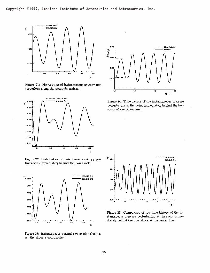
Figure 21: Distribution of instantaneous entropy per-turbations along the parabola surface.

i

Figure 22: Distribution of instantaneous entropy per-turbations immediately behind the bow shock.

Figure 24: Time history of the instantaneous pressureperturbation at the point immediately behind the bowshock at the center line.

160x120 Grid320x240 Grid

Figure 25: Comparison of the time history of the in-stantaneous pressure perturbation at the point imme-diately behind the bow shock at the center line.

Figure 23: Instantaneous normal bow shock velocitiesvs. the shock x coordinates.

26