DIRECT NUMERICAL SIMULATION OF A TRANSITIONAL JET IN CROSSFLOW WITH MIXING AND CHEMICAL REACTIONS

Jordan A. Denev Institute for Technical Chemistry und Polymer Chemistry,

University of Karlsruhe (TH) Kaiserstraße 12, D-76128 Karlsruhe

denev@ict.uni-karlsruhe.de

Jochen Fröhlich Institute for Fluid Mechanics, Technical University of Dresden,

George-Bähr Straße 3c, D-01062 Dresden, Germany jochen.froehlich@tu-dresden.de

Henning Bockhorn Institute for Technical Chemistry und Polymer Chemistry,

University of Karlsruhe (TH) Kaiserstraße 12, D-76128 Karlsruhe

bockhorn@ict.uni-karlsruhe.de

ABSTRACT The paper describes DNS of a jet in crossflow at

Re=650 and jet-to-crossflow velocity ratio R=3.3. Laminar boundary conditions are employed which makes the present flow configuration advantageous for benchmarking. Use is made of local grid refinement in the region of transition to turbulence. Comparison with Re=325 is carried out for some appropriate quantities. Nine passive scalars, reacting and non-reacting, are introduced. This allows to systematically study the influence of the Schmidt number and the Damköhler number with first order reactions. The presence of chemical reactions is a particular feature of the present study. Quantitative results for mean flow and turbulent quantities are provided and discussed. Also, the interaction between turbulence and scalar is quantified. Reference data are made available for later benchmarking.

INTRODUCTION The configuration of a jet issuing from a pipe into a

crossflow (JICF) appears frequently in chemical, pharmaceutical, environmental and combustion engineering, to name but a few application areas. The complex vortical structures of this flow and its good mixing capabilities make it a target of intense investigation for both experimental and numerical groups (Margason 1993). It is hence useful to consider such a situation as a benchmark configuration to assess statistical turbulence models as well as Large Eddy simulations (LES).

Earlier work of the present authors was concerned with turbulent inflow conditions of the jet (Fröhlich et al. 2004, Denev et al. 2005a, 2005b). In the present paper, the low-Reynolds number regime is considered with laminar pipe flow, where steady boundary conditions can be applied.

This is advantageous for two reasons: First, it removes the ambiguity of specifying in a benchmarking simulation the turbulent fluctuations at the inlet. Technical details in this respect may render comparisons of results from different groups difficult, as well as tracing deficiencies in a single computation back to a particular feature of the numerical method. Second, the transition of the jet from laminar to turbulent, now occurring inside the computational domain, provides a challenge for turbulence models (Denev et al. 2006).

Kelso et al. (1996) and Lim et al. (2001) performed experiments in the low-Reynolds number regime. They are however mainly concerned with flow visualization and analysis of coherent structures. Recent Direct Numerical Simulations (DNS) are reported by Muppidi and Mahesh (2005a, 2005b, 2006) for a case with velocity ratio R=u∞/wjet=5.7 and Reynolds number Rejet=wjetD/ν=5000, with “∞” indicating crossflow conditions and D the diameter of the pipe. This value of Rejet requires turbulent boundary conditions at some point upstream of the outlet of the jet. In the third of these references, a passive non-reactive scalar with Schmidt number Sc=1.49 was introduced with the jet.

The present work aims to supply a reference solution in a similar spirit which differs from the above simulations mainly in the following: (1) The Reynolds number is lower, such that the pipe flow is laminar. (2) Reacting and non-reacting passive scalars are introduced to provide reference data for mixing and chemical reactions. This feature is unique as there is no similar attempt in the literature the authors are aware of. The parameters have been selected such that the transition zone is short which is advantageous when used as benchmark to reduce the computational effort.

FLOW CONFIGURATION AND PARAMETERS

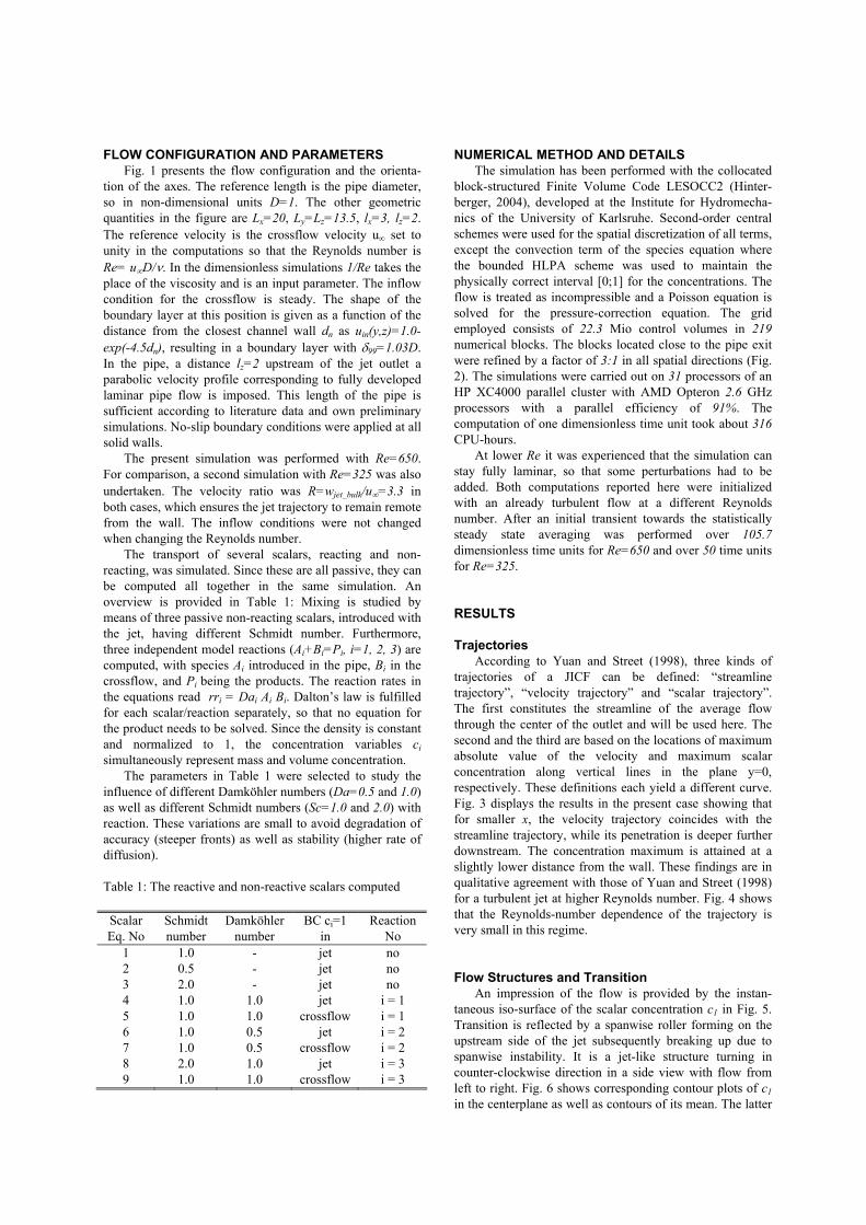
Fig. 1 presents the flow configuration and the orienta-tion of the axes. The reference length is the pipe diameter, so in non-dimensional units D=1. The other geometric quantities in the figure are Lx=20, Ly=Lz=13.5, lx=3, lz=2. The reference velocity is the crossflow velocity u∞ set to unity in the computations so that the Reynolds number is Re= u∞D/ν. In the dimensionless simulations 1/Re takes the place of the viscosity and is an input parameter. The inflow condition for the crossflow is steady. The shape of the boundary layer at this position is given as a function of the distance from the closest channel wall dn as uin(y,z)=1.0-exp(-4.5dn), resulting in a boundary layer with δ99=1.03D. In the pipe, a distance lz=2 upstream of the jet outlet a parabolic velocity profile corresponding to fully developed laminar pipe flow is imposed. This length of the pipe is sufficient according to literature data and own preliminary simulations. No-slip boundary conditions were applied at all solid walls.

The present simulation was performed with Re=650. For comparison, a second simulation with Re=325 was also undertaken. The velocity ratio was R=wjet_bulk/u∞=3.3 in both cases, which ensures the jet trajectory to remain remote from the wall. The inflow conditions were not changed when changing the Reynolds number.

The transport of several scalars, reacting and non-reacting, was simulated. Since these are all passive, they can be computed all together in the same simulation. An overview is provided in Table 1: Mixing is studied by means of three passive non-reacting scalars, introduced with the jet, having different Schmidt number. Furthermore, three independent model reactions (Ai+Bi=Pi, i=1, 2, 3) are computed, with species Ai introduced in the pipe, Bi in the crossflow, and Pi being the products. The reaction rates in the equations read rri = Dai Ai Bi. Dalton’s law is fulfilled for each scalar/reaction separately, so that no equation for the product needs to be solved. Since the density is constant and normalized to 1, the concentration variables ci simultaneously represent mass and volume concentration.

The parameters in Table 1 were selected to study the influence of different Damköhler numbers (Da=0.5 and 1.0) as well as different Schmidt numbers (Sc=1.0 and 2.0) with reaction. These variations are small to avoid degradation of accuracy (steeper fronts) as well as stability (higher rate of diffusion).

Table 1: The reactive and non-reactive scalars computed

Scalar Eq. No

Schmidt number

Damköhler number

BC ci=1 in

Reaction No

1 1.0 - jet no 2 0.5 - jet no 3 2.0 - jet no 4 1.0 1.0 jet i = 1 5 1.0 1.0 crossflow i = 1 6 1.0 0.5 jet i = 2 7 1.0 0.5 crossflow i = 2 8 2.0 1.0 jet i = 3 9 1.0 1.0 crossflow i = 3

NUMERICAL METHOD AND DETAILS

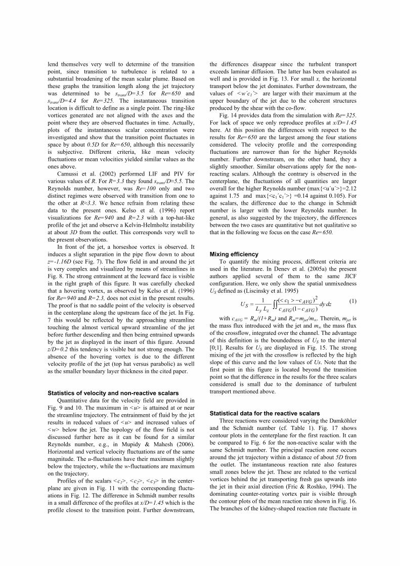
The simulation has been performed with the collocated block-structured Finite Volume Code LESOCC2 (Hinter-berger, 2004), developed at the Institute for Hydromecha-nics of the University of Karlsruhe. Second-order central schemes were used for the spatial discretization of all terms, except the convection term of the species equation where the bounded HLPA scheme was used to maintain the physically correct interval [0;1] for the concentrations. The flow is treated as incompressible and a Poisson equation is solved for the pressure-correction equation. The grid employed consists of 22.3 Mio control volumes in 219 numerical blocks. The blocks located close to the pipe exit were refined by a factor of 3:1 in all spatial directions (Fig. 2). The simulations were carried out on 31 processors of an HP XC4000 parallel cluster with AMD Opteron 2.6 GHz processors with a parallel efficiency of 91%. The computation of one dimensionless time unit took about 316 CPU-hours.

At lower Re it was experienced that the simulation can stay fully laminar, so that some perturbations had to be added. Both computations reported here were initialized with an already turbulent flow at a different Reynolds number. After an initial transient towards the statistically steady state averaging was performed over 105.7 dimensionless time units for Re=650 and over 50 time units for Re=325.

RESULTS

Trajectories

According to Yuan and Street (1998), three kinds of trajectories of a JICF can be defined: “streamline trajectory”, “velocity trajectory” and “scalar trajectory”. The first constitutes the streamline of the average flow through the center of the outlet and will be used here. The second and the third are based on the locations of maximum absolute value of the velocity and maximum scalar concentration along vertical lines in the plane y=0, respectively. These definitions each yield a different curve. Fig. 3 displays the results in the present case showing that for smaller x, the velocity trajectory coincides with the streamline trajectory, while its penetration is deeper further downstream. The concentration maximum is attained at a slightly lower distance from the wall. These findings are in qualitative agreement with those of Yuan and Street (1998) for a turbulent jet at higher Reynolds number. Fig. 4 shows that the Reynolds-number dependence of the trajectory is very small in this regime.

Flow Structures and Transition

An impression of the flow is provided by the instan-taneous iso-surface of the scalar concentration c1 in Fig. 5. Transition is reflected by a spanwise roller forming on the upstream side of the jet subsequently breaking up due to spanwise instability. It is a jet-like structure turning in counter-clockwise direction in a side view with flow from left to right. Fig. 6 shows corresponding contour plots of c1 in the centerplane as well as contours of its mean. The latter

lend themselves very well to determine of the transition point, since transition to turbulence is related to a substantial broadening of the mean scalar plume. Based on these graphs the transition length along the jet trajectory was determined to be strans/D=3.5 for Re=650 and strans/D=4.4 for Re=325. The instantaneous transition location is difficult to define as a single point. The ring-like vortices generated are not aligned with the axes and the point where they are observed fluctuates in time. Actually, plots of the instantaneous scalar concentration were investigated and show that the transition point fluctuates in space by about 0.5D for Re=650, although this necessarily is subjective. Different criteria, like mean velocity fluctuations or mean velocities yielded similar values as the ones above.

Camussi et al. (2002) performed LIF and PIV for various values of R. For R=3.3 they found strans/D≈5.5. The Reynolds number, however, was Re=100 only and two distinct regimes were observed with transition from one to the other at R≈3.3. We hence refrain from relating these data to the present ones. Kelso et al. (1996) report visualizations for Re=940 and R=2.3 with a top-hat-like profile of the jet and observe a Kelvin-Helmholtz instability at about 3D from the outlet. This corresponds very well to the present observations.

In front of the jet, a horseshoe vortex is observed. It induces a slight separation in the pipe flow down to about z=-1.16D (see Fig. 7). The flow field in and around the jet is very complex and visualized by means of streamlines in Fig. 8. The strong entrainment at the leeward face is visible in the right graph of this figure. It was carefully checked that a hovering vortex, as observed by Kelso et al. (1996) for Re=940 and R=2.3, does not exist in the present results. The proof is that no saddle point of the velocity is observed in the centerplane along the upstream face of the jet. In Fig. 7 this would be reflected by the approaching streamline touching the almost vertical upward streamline of the jet before further descending and then being entrained upwards by the jet as displayed in the insert of this figure. Around z/D=0.2 this tendency is visible but not strong enough. The absence of the hovering vortex is due to the different velocity profile of the jet (top hat versus parabolic) as well as the smaller boundary layer thickness in the cited paper.

Statistics of velocity and non-reactive scalars Quantitative data for the velocity field are provided in

Fig. 9 and 10. The maximum in <u> is attained at or near the streamline trajectory. The entrainment of fluid by the jet results in reduced values of <u> and increased values of <w> below the jet. The topology of the flow field is not discussed further here as it can be found for a similar Reynolds number, e.g., in Mupidy & Mahesh (2006). Horizontal and vertical velocity fluctuations are of the same magnitude. The u-fluctuations have their maximum slightly below the trajectory, while the w-fluctuations are maximum on the trajectory.

Profiles of the scalars <c1>, <c2>, <c3> in the center-plane are given in Fig. 11 with the corresponding fluctu-ations in Fig. 12. The difference in Schmidt number results in a small difference of the profiles at x/D=1.45 which is the profile closest to the transition point. Further downstream,

the differences disappear since the turbulent transport exceeds laminar diffusion. The latter has been evaluated as well and is provided in Fig. 13. For small x, the horizontal transport below the jet dominates. Further downstream, the values of <w´c1´> are larger with their maximum at the upper boundary of the jet due to the coherent structures produced by the shear with the co-flow.

Fig. 14 provides data from the simulation with Re=325. For lack of space we only reproduce profiles at x/D=1.45 here. At this position the differences with respect to the results for Re=650 are the largest among the four stations considered. The velocity profile and the corresponding fluctuations are narrower than for the higher Reynolds number. Further downstream, on the other hand, they a slightly smoother. Similar observations apply for the non-reacting scalars. Although the contrary is observed in the centerplane, the fluctuations of all quantities are larger overall for the higher Reynolds number (max{<u´u´>}=2.12 against 1.75 and max{<c1´c1´>} =0.14 against 0.105). For the scalars, the difference due to the change in Schmidt number is larger with the lower Reynolds number. In general, as also suggested by the trajectory, the differences between the two cases are quantitative but not qualitative so that in the following we focus on the case Re=650.

Mixing efficiency To quantify the mixing process, different criteria are

used in the literature. In Denev et al. (2005a) the present authors applied several of them to the same JICF configuration. Here, we only show the spatial unmixedness US defined as (Liscinsky et al. 1995)

∫∫ −−><

= dzdycc

ccLL

UAVGAVG

AVG

zyS )1(

)(1 21 (1)

with cAVG = Rm/(1+Rm) and Rm=mjet/m∞. Therein, mjet is the mass flux introduced with the jet and m∞ the mass flux of the crossflow, integrated over the channel. The advantage of this definition is the boundedness of US to the interval [0;1]. Results for US are displayed in Fig. 15. The strong mixing of the jet with the crossflow is reflected by the high slope of this curve and the low values of Us. Note that the first point in this figure is located beyond the transition point so that the difference in the results for the three scalars considered is small due to the dominance of turbulent transport mentioned above.

Statistical data for the reactive scalars Three reactions were considered varying the Damköhler

and the Schmidt number (cf. Table 1). Fig. 17 shows contour plots in the centerplane for the first reaction. It can be compared to Fig. 6 for the non-reactive scalar with the same Schmidt number. The principal reaction zone occurs around the jet trajectory within a distance of about 5D from the outlet. The instantaneous reaction rate also features small zones below the jet. These are related to the vertical vortices behind the jet transporting fresh gas upwards into the jet in their axial direction (Fric & Roshko, 1994). The dominating counter-rotating vortex pair is visible through the contour plots of the mean reaction rate shown in Fig. 16. The branches of the kidney-shaped reaction rate fluctuate in

time and generate the reaction zone below the jet in Fig. 17. The inward motion of the mean flow into the jet is also seen in the right graph of Fig. 8.

Fig. 18 reports the reaction rates quantitatively. It is seen that the third reaction proceeds as the first one, hence that lower diffusion of the jet scalar does not have a sizable impact. Fig. 19 shows the resulting mean concentrations for c4 and c5 and compares them to the non-reacting c1. The corresponding fluctuations are reported in Fig. 20.

CONCLUSIONS Direct Numerical Simulations have been reported for a

jet into a crossflow at Reynolds number 650 and 325. Several reactive and non-reactive passive scalars were intro-duced and analyzed. The setup provides reference data for the validation of turbulence models in the challenging situa-tion of transitional flow and also for reactive flow. Models of the latter are delicate because of the interaction between reaction rate and turbulence. The importance of turbulent transport is demonstrated by the similarity of the results when changing the Reynolds number in the present simulations.

Quantitative results for all processes were presented which, due to the limited space, were restricted to the centerplane here. All data are available as downloads from http://www.ict.uni-karlsruhe.de/index.pl/themen/dns/index.html. Currently, an experimental campaign is undertaken at the University of Karlsruhe to provide experimental data for a very similar configuration. AKNOWLEDGEMENTS

This research was funded by the German Research foundation through priority programme SPP-1141 "Mixing devices". Carlos Falconi helped with preparing figures.

REFERENCES

Camussi, R., Gui, G., and Stella, A., 2002, “Experimen-tal study of a jet in a crossflow at very low Reynolds num-ber”, J. Fluid Mech., vol. 454, pp. 113-144.

Denev, J.A., Fröhlich, J., and Bockhorn, H., 2005a, “Evaluation of mixing and chemical reactions within a jet in crossflow by means of LES”, Proc. of European Combustion Meeting, Belgium.

Denev, J.A., Fröhlich, J., and Bockhorn, H., 2005b, “Structure and mixing of a swirling transverse jet into a crossflow”, Procs. of 4th Int. Symp. on Turbulence and Shear Flow Phenomena, USA, vol. 3, pp. 1255-1260.

Denev, J.A., Fröhlich, J., and Bockhorn, H., 2006, “Di-rect numerical simulation of mixing and chemical reactions in a round jet into a crossflow”, High Performance Computing in Science and Engineering 06, Transactions of the HLRS Stuttgart, Nagel, W.E. et al. (eds.), Springer, pp. 237-251.

Fric, T.F., and Roshko, A., 1994, “Vortical structure in the wake of a transverse jet”, J. Fluid Mech., vol. 279, pp. 1-47.

Fröhlich, J., Denev, J.A., and Bockhorn, H., 2004, “Large eddy simulation of a jet in crossflow”, Proc. of 4th Eur. Congr. on Comput. Meth. Appl. Sci. Engi, ECCOMAS 2004, Finland.

Hinterberger, C., 2004, „Dreidimensionale und tiefenge-mittelte Large–Eddy–Simulation von Flachwasserströmun-gen”, PhD thesis, Inst. Hydromechanics, Univ. of Karlsruhe.

Kelso, R.M., Lim, T.T., and Perry, A.E., 1996, “An experimental study of round jets in cross-flow”, J. Fluid Mech., vol. 306, pp 111-144.

Lim T.T., New T.H., and Luo, S.C., 2001, “On the development of large-scale structures of a jet normal to a cross flow. Phys. Fluids, vol. 13 pp 770-775.

Liscinsky, D.S., True, B. and Holdeman, J.D., 1995, “Effects of Initial Conditions on a Single Jet in Crossflow”, 31st Joint Propulsion Conference and Exhibit, San Diego, California, July 10-12, AIAA Paper 1995-2998.

Margason, R.J. 1993. “50 years of Jet in Cross Flow Research” AGARD-CP 534, pp. 1.1-1.41.

Muppidi, S., and Mahesh, K., 2005a, “Study of trajectories of jets in crossflow using direct numerical simulations”, J. Fluid Mech., vol. 520, pp. 81-100.

Muppidi, S., and Mahesh, K., 2005b, “Velocity field of a round turbulent transverse jet”, Procs. 4th Int. Symp. on Turbulence and Shear Flow Phenomena, J.A.C. Humphrey, T.B. Gatski, J.K. Eaton, R. Friedrich, N. Kasagi, and M.A. Leschziner (Eds.), Williamsburg, vol. 2, pp. 829-833.

Muppidi, S., and Mahesh, K., 2006, “Passive scalar mixing in jets in crossflow”, 44th AIAA Aerospace Sciences Meeting and Exhibit, Reno, Nevada, Jan 9-12, AIAA Paper 2006-1098.

Yuan, L. L., and Street, R. L., 1998, “Trajectory and entrainment of a round jet in crossflow”, Phys. Fluids, vol. 10(9), pp. 2223-2335.

Fig. 1: Geometry of the computational domain.

Fig. 2: Locally refined grid near the jet exit.

Fig. 3: Streamline trajectory in the center plane for

Re=650 compared to the scalar-based and velocity-based trajectory.

Fig. 4: Trajectories for the two Reynolds numbers

considered.

Fig. 5: Instantaneous iso-surface c1=0.18.

Fig. 6: Transition point visualized by the scalar c1. Left: instantaneous values, right: mean value. Thin

white line inserted manually. Top: Re=650, bottom: Re=325.

Fig. 7: Zoom in the centerplane at the windward side

of the outlet showing the horseshoe vortex and the backflow in the pipe. The small right insert after Kelso et al. (1996) indicates how the hovering vortex (HV) would show up

together with a saddle point (SP).

Fig. 8: Streamlines of the mean flow field related to

the iso-surface <c1>=0.15 (left) and to an iso-surface of mean velocity magnitude equal to 1.65.

Fig. 9: Mean velocity <u> and <w> in the centerplane.

Fig. 10: Velocity fluctuations (RMS) in the centerplane.

Fig. 11: Mean scalar concentrations of the non-reacting

scalars in the centerplane.

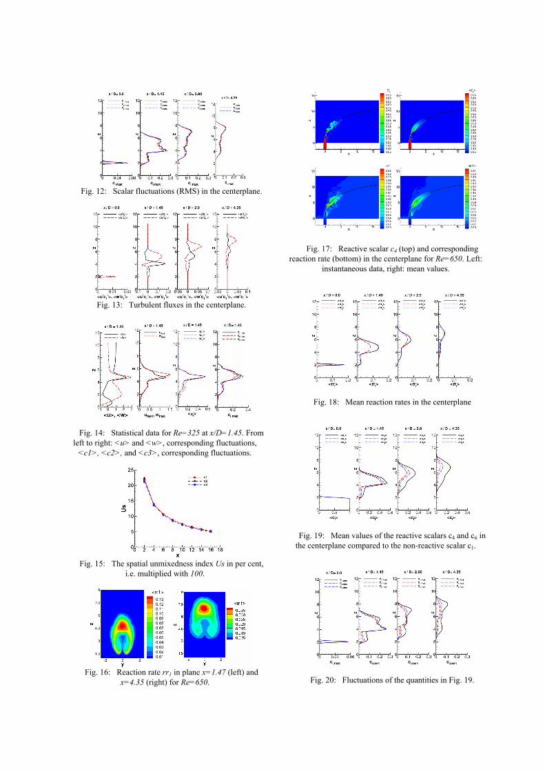
Fig. 12: Scalar fluctuations (RMS) in the centerplane.

Fig. 13: Turbulent fluxes in the centerplane.

Fig. 14: Statistical data for Re=325 at x/D=1.45. From left to right: <u> and <w>, corresponding fluctuations,

<c1>, <c2>, and <c3>, corresponding fluctuations.

Fig. 15: The spatial unmixedness index Us in per cent,

i.e. multiplied with 100.

Fig. 16: Reaction rate rr1 in plane x=1.47 (left) and

x=4.35 (right) for Re=650.

Fig. 17: Reactive scalar c4 (top) and corresponding reaction rate (bottom) in the centerplane for Re=650. Left:

instantaneous data, right: mean values.

Fig. 18: Mean reaction rates in the centerplane

Fig. 19: Mean values of the reactive scalars c4 and c6 in the centerplane compared to the non-reactive scalar c1.

Fig. 20: Fluctuations of the quantities in Fig. 19.