JOURNAL OF GUIDANCE, CONTROL, AND DYNAMICS

Vol. 23, No. 5, September–October 2000

Direct Method for Rapid Prototypingof Near-Optimal Aircraft Trajectories

Oleg A. Yakimenko¤

Aviation and Aeronautics Academy of Sciences, Moscow, 125190, Russia

A direct method for a real-time generation of near-optimal spatial trajectories of short-term maneuvers onboarda � ying vehicle with predetermined thrust history is introduced. The paper starts with a survey about the foundersof the direct methods of calculus of variations and their followers in � ight mechanics, both in Russia and inthe United States. It then describes a new direct method based on three cues: high-order polynomials from thevirtual arc as a reference function for aircraft’s coordinates, a preset history of one of the controls (thrust), and afew optimization parameters. The trajectory optimization problem is transformed into a nonlinear programmingproblem and then solved numerically using an appropriate algorithm in accelerated scale of time. A series ofexamples is presented. Calculated near-optimal trajectory is compared with real � ight data, and with the solutionobtainedbyPontryagin’s maximumprinciple.Fast convergenceof the numerical algorithm,which hasbeen alreadyimplemented and tested onboard a real aircraft, is illustrated.

Nomenclatureaik = polynomial coef� cientsg = acceleration due to gravityJ = cost functionj = quantity pertaining to the j th time nodem = aircraft massN = number of nodesn = polynomial ordern = relative revolutions of engine’s rotornx , nz = tangential and normal projections of load factor,

respectivelySh = penalty functionT , T = total thrust and relative thrust (fraction of maximum

thrust), respectivelyt = timet ¤T ( s ¤

T ) = thrust-off instant (arc)t ¤ ¤T ( s ¤ ¤

T ) = thrust-on instant (arc)V = airspeedxi = aircraft mass center coordinates in the Earth

north-east-downinertial frame, i = 1, 2, 3a = angle of attackc , v = � ightpath and azimuth angles, respectivelyD s , D t j = sampling periodd T = throttle position´, », ¼ = sets of restrictionson state variables, controls, and their

time derivativesk = virtual velocity along the virtual arcN = vector of optimization parameterss = virtual arcu = bank angle in wind frameX f = vector of “free” (not preset) terminal states and controls0 , 0 0 , 0 0 0 = arc derivatives¢ , ¢ ¢ , ¢ ¢ ¢ = time derivatives

¯ = relative parameter

I. Background

A CONCEPT of the onboard pilot’s support system (PSS; elec-troniccopilotor pilot associate) assumes the presenceof a sub-

Received 17 May 1999; revision received 18 January 2000; accepted forpublication 1 February 2000. Copyright c° 2000 by Oleg A. Yakimenko.Published by the American Institute of Aeronautics and Astronautics, Inc.,with permission.

¤ Corresponding Member of AAAS; currently National Research Coun-cil Senior Research Associate–Visiting Professor at the Naval PostgraduateSchool, Code AA/YK, 699 Dyer Road, Monterey, CA 93943; oayakime@nps.navy.mil. Senior Member AIAA.

system for pilot’s control actions during maneuvering support.1 Forsome standard maneuvers, this subsystem is built on the databasesof near-optimal trajectoriescalculated beforehand.2 These trajecto-ries banks (TBs) as banks of good initial guesses make it possibleto reconstruct the spatial near-optimalPSS-suggested trajectory forthe real tactical situation (in other words, to make a � nal onboardoptimization), and to visualize this trajectory for a pilot at head-up/head-down display (HUD/HDD). The main control mode, at therequest of pilots, must become “the director with sight” controlmode.3

Modern indirect methods of mathematical theory of optimalprocesses4 ¡ 6 reduce the problemof cost function (CF) optimizationto solutionof the two-point boundary-valueproblem. However, thisapproach is not always effective,especially in the task under consid-eration, and this approach is greatly complicated because we needto solve a given variational problem not in a small neighborhoodof some point (as is usually the case in the theory of differentialequations), but rather a solution in some � xed region. Moreover,it is well known that differential equations of variational problemscan be integrated easily only in exceptional cases, e.g., the two-point boundary value problem is very dif� cult to solve for all butthe simplest problems (only in a vertical or horizontal plane withsimpli� cation of state equations and with a rather simple CF).

Dif� culties inherent in this approachhave led to a search for vari-ational methods of a differentkind, known as direct methods,whichdo not entail the reduction of variational problems to problems in-volving differentialequations.According to Ewing7 the term directmethods was applied to the approach for the existence theory ini-tiated by Hilbert (as it was written by Bolza8 in the beginning ofthe century) and was developedby Tonelli,9 and others. The funda-mental idea of direct methods is to consider a variational problemas a limit problem of the extreme of a function of a � nite number ofvariables to be solved by usual methods. Because of their conver-gence robustness,direct methods give the safest approach for rapidprototyping of spatial trajectories for a � ying vehicle (FV).10

II. IntroductionThe main idea of the direct methods is to consider a function as a

� nite set of variables. This is fairly evident if it is assumed that theadmissible functioncan be representedby an in� nitive power series

y(x ) =1

k = 0

ak x k

or by a Fourier series

y(x) =a0

2+

1

k = 1

(ak coskx + bk sin kx )

865

866 YAKIMENKO

or by any series of the form

y(x ) =1

k = 0

ak } k (x )

where } k (x ) are given functions. Then a CF will be the functionof a set of unknown coef� cients, allowing us to reduce the task byconsidering a � nite series instead of in� nite.11

It was Euler12 who applied for � rst time, a method, which is nowcalled the directmethodof � nite differences(after Euler appliedit, itwasn’t in use for a long time, but in the last decades, beginningwithLusternik,Petrovskiyandothers, it hasbeenusedwidely).11 Anotherdirect method is a method by Ritz,13 which after the methods ofKrylov14 and Bogolubov, is of wide use in the theory of elasticity.14

The Ritz procedure requires a � eld problem to be set up as anintegral minimization.Thus it can be applied to problems for whicha variationalprinciple exists. There are, however, other methods ofdetermining the unknown coef� cients in the approximating func-tion that operate directly on the governing differential equation.This more simple but more universal procedure was introducedby Galerkin15 as a means of obtaining approximate solutions toboundary-value problems. When combined with the interpolationequations of the method of � nite elements, which is a variation ofthe Rayleigh–Ritz procedure, Galerkin’s method becomes a veryuseful procedure for solving both initial and boundary-valueprob-lems. Galerkin used a direct method for the solution of parabolicand elliptic partial differential equations.

The � nite element method was � rst conceived and used byaerospace engineers in the early 1950s. Because of the improve-ment of computers during the following years, this method becamemore popular for numerical simulation for a large range of physi-cal problems written in terms of partial differential equations, e.g.,stress analysis, structural and solid mechanics, heat transfer, � uidmechanics, and others. The method of Kantorovich16 applies to CFsthat depend on functions of several independent variables.

As mentioned in Ref. 11, the question of convergence of Euler,Ritz, and others’ approximations to the desired solution of a varia-tional problem, as well as the problem of estimationof the degreeofapproximation,is very complicated.The discussionof this matter isoutside the scopeof this paper;however, some proof of convergenceof Euler or Ritz approximationscan be found, for instance, in Refs.7, 16, 17. Nevertheless, at least, we can state that direct methodsyield approximation of the minima from above (or maxima frombelow). Therefore, we can regard them as rapid prototyping of op-timal solutions (or near-optimal solution). These methods, whichuse direct presetting of extremal trajectories and/or controls, give ahuge calculationadvantage and can provide a near-optimalsolutionwith any desired accuracy.

It was Taranenko,18 who developed and applied a method likeRitz–Galerkin to the problems of � ight mechanics with constraintson state variables and controls. Following the main idea of thedirect methods, Taranenko suggested de� ning the reference func-tions for both FVs Cartesian coordinates (xi , i = 1, 2, 3) and its air-speed (x4 ´ V ) as xi = xi0 + (xi f ¡ xi0)( s ¡ s 0 )/ ( s f ¡ s 0 ) + U i ( s )(i = 1, 2, 3, 4).18 Here s is an argument, and U i ( s ) are continu-ous, unequivocal,and differentiablefunctions satisfying to obviousboundary conditions U i ( s 0) = U i ( s f ) ´ 0. Taranenko proposed touse one of the following functions:

U 1i ( s ) =

n

k = 1

Ak sin k ps ¡ s 0

s f ¡ s 0

or

U 2i ( s ) =

n

k = 1

Ak ( s ¡ s 0 )k ( s ¡ s f )k

or U 3i ( s ) = ( s ¡ s 0 )m1 ( s ¡ s f )m2 , or their linear combination.How-

ever, in principle, there are no limitations, and one can use any con-venient functions for the particular task under consideration (seeexample in Ref. 19). Other state parameters and controls are thendetermined through the solution of the inverse problem of � ightdynamics. (The inverse problem means that we have to de� ne the

controls time histories that provide a desired reference trajectory,whereas a direct problem deals with calculation of FVs trajectoryat known initial state variablesand controls time histories, meaningthe Cauchy task.)

An explicit mean to increase � exibility is to increase a num-ber of elements n in a series U 1

t ( s ), U 2i ( s ), or to increase powers

m1 and m2 in U 3i ( s ). However, Taranenko proceeded with another

approach—he subdivided an interval [s 0; s f ] on several pieces andemployed low-order polynomials to describe a behavior of statevariables xi (i = 1, 2, 3, 4) along each of them [the parameters ofpieces’ collocation can then be considered as an additional opti-mization parameter (OP)]. The higher number n (or m1 and m2),and the higher the number of pieces in piecewise case, the closer anear-optimal solution is to the optimal one.11

The choice of an argument s also depends on a particular task.Generally speaking, one can use any continuousmonotonic param-eter: time, path, sometimes total mechanical energy, and others.However, it is obvious that in case of de� ning both FV’s coordi-nates and airspeed, as Taranenko did, we should use any abstractparameter; otherwise we will be unable to vary trajectory and speedhistory independently.Taranenko called s a virtual arc.18

Taranenko and Momdzhi20 and their followers � nally preferredthe sum of three cubic polynomials as reference functions:

xi ( s ) =3

k = 0

aik s k +5

k = 4

ai k( s ¡ s k ¡ 3,i )3 @ j ¡ 3,i

@ k ¡ 3,i =0 if s · s k ¡ 3,i

1 if s > s k ¡ 3,i, i = 1, 2, . . . , 4

where coef� cients ai k are automatically de� ned by preset bound-ary conditions at the origin and the end of the trajectory.Taranenkochose the cubic splines to be able to satisfy boundary conditionsimposed on state variables, their � rst and second derivatives (thirdderivative in this case is discontinuous). In the case of control’sconstraint violation, they switch on direct integration of the stateequations with the marginal value of this (violated) control. Sincethe 1960s, with the use of this method, a lot of optimization prob-lems have been solved for differentFV, includinghelicopters,strikeaircraft,civil aircraft,airspacevehicle,e.g., such problemsas climb-to-dash, orbit maneuvering, descent from the orbit, surface-basedtarget attack (SBTA) approach, curved landing approach (CLA).Blagodarniy21 used these functions to optimize a series of ma-neuvers with preset intermediate points. Akulov and Schisljonok22

added trigonometric functions U 1i ( s ) to be able to optimize helix-

type maneuvers.Neljubov23 used 5–7 order time-polynomials for Cartesian co-

ordinates only and implemented them as basic trajectories duringthe following tracking with real automatics. With the use of thisapproach, a number of practical optimization problems was alsosolved for different stages of � ight and for different FV.

However, the analysisof thesemethods shows that they cannotbeused directly to create and handleTBs for onboardon-lineoptimiza-tion. The method by Taranenkoand Momdzhi20 has relativelymanyOPs (in general, 10 of them) that cause insuf� cient performance inthe calculation of the optimal trajectory, even with a good initialguess. At the end of the trajectory, the third derivatives of the statevariables cannot be speci� ed; as a result, the obtained trajectory isoftendif� cult to trackin a manual (directorwith sight) controlmode.A trajectorypartiallypassingalong the normal load factor constraintis also hard to realize; in addition, this part of the trajectoryassumesdirect integration of state equations that not only slows down theiteration process, but also makes it impossible to have an analyticalpresentationof the entire trajectory.The approachof Neljubov23 as-sumes the trackingof the basic trajectoriesby means of automation.As a result, the obtained near-optimal trajectory is no longer ana-lytical at all, and may substantiallydiffer from the basic trajectory.Consequently, these basic trajectoriescannot be proposed to a pilotas the reference ones for their tracking.

Another branch of direct methods deal with discretization ofa continuous problem reducing the initial variational problem to

YAKIMENKO 867

the problem of optimization of parameters, de� ning state variablesand/or controls in this sampling point, which means without globalanalytical approximation of states’ (controls’) histories.

Hargraves and Paris,24 von Stryk and Bulirsch,25 Convay andcolleagues,26,27 Betts,28 Calise and Leung,29 Hull,30 and othersused the so-called collocation-based or direct transcription meth-ods, which are similar in many respects to Galerkin’s procedure.They reduce the initial problem by segmenting the time intervalinto the 5–20 pieces and representing the solution both for statevariables and controls by piecewise polynomials (constants). Thetens of unknown coef� cients are then determined by enforcingcon-tinuity at the nodes and by satisfying the differential equationsat some speci� ed points in each segment (along with Ritz’s andGalerkin’s methods, this is the third known way of obtaining un-known coef� cients). Seywald and Kumar31 ¡ 33 and others used theso-called differential inclusion approach. They eliminated controlsfrom the state equations by employing a description of the dynam-ical system in terms of its attainable set. The previously mentionedprocedure can permit the reduction of the size of the parameteroptimization problem.33,34 Smaller problems can then be solvedmore quickly. Lu35,36 used, for each piece, an approach similar toTaranenko’s method. Following Refs. 37 and 38, he called it theinverse dynamics approach. For optimization of planar trajectoryfor an aerospace vehicle at each of the 20 pieces he preset one ofthe state variables’ time history and one of the controls’ time his-tory by cubic splines, and then he solved the inverse task of � ightdynamics.

These approaches imply relatively dif� cult numerical calcula-tions with numerous OPs with the help of gradient methods, whichrequire a good initial guess. Their accuracy directly depends on thenumber of segments used in the approximation.Nevertheless, thesemethods are effectively used for off-line optimization of long-termplanar maneuversof aerospaceFVs, such as launch trajectories,or-bit rendezvous and transfer problems, and climb-to-dash. Actually,these methodswere developednamely for these applications,so thatthe small changesintroducedearly in the trajectorydo notpropagateto the end of the trajectory.

Although all of the cited direct approaches intuitively applyingthe same fundamental ideas havebeen successfullyused for off-linetrajectoriesoptimization,33 nobodyhas developedand implementedthe direct method for on-line (real-time) optimizationof short-termspatial trajectoriesfor a highmaneuverableaircraft.Becauseit is im-possible to use alreadydesignednumericalschemes for the problemat hand, the present paper deals with a new, in some sense, simpli-� ed method that provides rapid prototyping of near-optimal spatialtrajectoriesbeing presented analyticallyand completely de� ned byseveral OPs. Besides, for further improvement of convergence ro-bustness, it is possible and easy to implement an idea of TBs.2,4

This method combines a number of advantages over methodsby Taranenko and Momdzhi20 and Neljubov,23 and consequently aclose position to Lu’s approach.35 Though having less possibilitiesof varying the trajectory itself (with the goal of � nding an optimalone), this algorithm assures the following: the boundary conditionsare satis� ed a priori; an aircraft control is physical and realizable(smooth), meaning a pilot can easily perform it; the iterative pro-cess converges well, making it possible to proceed with on-lineoptimization; the near-optimal solution is close enough to the opti-mal one. These features allowed this method to be employed on anIBM486-type computer and to be � ight tested onboard of the � y-ing laboratory Antonov-72 in the Gromov’s State Flight-ResearchInstitute,Zhukovkiy,Russia, in the spring of 1997 in real time. Ref-erence CLA-type trajectorieshad been computed not slower than inone-two seconds, visualizedon the HUD in the view of the Tunnel-in-Sky image,2 and successfully tracked by pilots.

The present paper deals with the mathematical foundation of di-rect method for rapid prototyping (DMRP) and is organized as fol-lows. The trajectory optimization problem as well as the modelof an aircraft is described in Sec. III. Section IV introduces thecomputational algorithm, and Sec. V deals with simulation results.Section V also containsa comparisonof obtained solutionswith thePontryagin’s maximum principle (PMP) and � ight test data. Somenear-optimal solutions for different tasks are also discussed here.

Justi� cation of method convergence robustness and the implemen-tation of TB ideas are illustrated as well.

III. Problem De� nition and General RelationsA. Trajectory Optimization Problem

The most general statement of the optimal control problem, de-terminingFV trajectoryfrom the current point to a given point, maybe speci� ed as follows.

There is a set of admissible trajectories:

z(t ) = {z1(t ), z2(t ), . . . , zr (t )}T 2 S

S = { z(t ) 2 Z r ½ E r }, t 2 b t0 , t f c

satisfying:1) the system of ordinary differential equations:

Çzi = fi (t, z, u, c), i = 1, 2, . . . , r (1)

where u(t ) ={u1(t ), u2(t ), . . . , ul (t )}T , l < r , u 2 U l ½ E l is thevector of controls, and c = (c1 , c2, . . . , cp ), c 2 C p ½ E p is the vec-tor of FV technical characteristics;

2) initial conditions:

z(t0) ´ z0 2 S0, S0 z0 2 Z r ½ E r (2)

u(t0) ´ u0 2 R0, R0 = u0 2 U l ½ E l (3)

and � nal (terminal) conditions:

z(t f ) ´ z f 2 S f , S f z f 2 Z r ½ Er (4)

u(t f ) ´ u f 2 R f , R f = u f 2 U l ½ E l (5)

3) restrictions on the state space:

´(t, z) = {g 1(t, z), g 2(t, z), . . . , g w (t , z)}T ¸ 0 (6)

on controls:

»(t, z, u) = {n 1(t, z, u), n 2(t , z, u), . . . , n v (t, z, u)}T ¸ 0 (7)

and on their derivatives:

¼(t, u, Çu) = {p 1(t, u, Çu), p 2(t , u, Çu), . . . , p r (t, u, Çu)}T ¸ 0 (8)

The problemis to � nd an optimal trajectoryzopt(t ) that minimizessome CF J and an optimal control uopt(t ) corresponding to thistrajectory.

Although in the preceding de� nition of the problem a terminalpoint is considered as completely de� ned [see Eqs. (4) and (5)]; ingeneral, some state variables and/or controls at the � nal point maynot be preset. In this case, as all direct methods do, the set of these“free” variables X f is assumed as additional OPs. Moreover, for acombat aircraft, the CF can be represented not only as integratedfunction

J =t f

t0

f0(t, z, u) dt

(the simplest examples are maneuver time or fuel consumption),but also as the function of current coordinates and controls inthe terminal point or at some event-conditioned instant of timet ¤ ( q (t ¤ , z, u) = 0) J = F (z, u)j t ¤ , e.g., terminal load factor or bankangle at aiming point.

868 YAKIMENKO

B. Aircraft ModelAs a system (1), considerthe three-dimensionalpoint-massequa-

tions over a � at Earth with zero sideslip angle:

Çx1 = V cos c cos v , ÇV = g(nx ¡ sin c )

Çx2 = V cos c sin v , Çc = (g / V )(nz cos u ¡ cos c )

Çx3 = ¡ V sin c , Çv = (g / V cos c )nz sin u , Çm = ¡ Cs (9)

where

nx = [T (d T , n)Tmax(M , x3, c) cos( a + e T ) ¡ D( a , M , x3 , c)]/ mg(10)

nz = [T (d T , n)Tmax(M , x3 , c) sin( a + e T ) + L( a , M , x3 , c)]/ mg(11)

and

Çn =kT d T ¡ n

td (n)(12)

In Eqs. (9) Cs(M , x3, c) denotes a fuel � ow rate; in Eqs. (10) and(11) e T denotes a thrust vector incidence angle, terms L and D arethe aerodynamic lift and drag, and M denotes the Mach number.Terms kT and td in Eq. (12) correspond to engine characteristics(gain and delay).

Consider the vector z ={x1 , x2, x3, V , c , v }T as a vector of statevariables with corresponding Eqs. (5)-type constraints on altitude( ¡ x3) and speed (V ), and the vector u ={d T , nz( a ), u }T as a vectorof controls. The constraints on controls of the Eq. (7)-type are asfollows:

d T 2 [d T min; d T max] nz 2 [nz min; nz max(M , x3 )] j u j · u max

where a normal load-factor projection accounts for both aerody-namic (nCL

z ) and structural(nstrz ) constraints.The constraintson their

derivatives[Eq. (8)-type] take into account thrust built-upand trust-decay times [through Eq. (12)] and the characteristicsof an aircraftcontrol system (constraints on Çnz and Çu ).

The aircraft models used in this study were representatives ofstrike aircraft like A-10 “Thunderbolt” (Su-25 “Frogfoot”) andhigh-performance multirole � ghters like F-16 “Falcon” (Su-27“Flanker”). Their nonlinear aerodynamic characteristics were pre-sented by corresponding coef� cients de� ned by multidimensionaltabulated data. Propulsion performance was also given by two-dimensional tables from x3 and M for different n. Linear interpo-lation was used for look-up. The atmospheric density was assumedto be a power function of altitude (for x3 ¸ ¡ 11 km).

IV. Computational AlgorithmA. Reference Functions for Aircraft Coordinates

We take the reference functions for aircraft coordinates xi (i =1, 2, 3) as algebraic polynomials of degree n with the virtual arc sas an argument, thus making it possible to optimize independentlythe velocity history along the trajectory:

xi ( s ) =n

k = 0

ai k(max(1, k ¡ 2))!s k

k!

x 0i ( s ) =

n

k = 1

aik(max(1, k ¡ 2))!s k ¡ 1

(k ¡ 1)!

x 0 0i ( s ) =

n

k = 2

aik s k ¡ 2, x 0 0 0i ( s ) =

n

k = 3

(k ¡ 2)aik s k ¡ 3 (13)

The degree n of these polynomials is determined by the numberof boundaryconditionsto be met, so that all coef� cientsai k were de-termined algebraically,rather than varied.The higher the maximumdegree of time derivative of an aircraft coordinate at initial and ter-minal points, whose values (the derivatives) are known, the higherthe degree of the polynomial. The minimum degree of the polyno-mial is n = d0 + d f + 1, which is greater by one than the sum of the

maximum orders of the time derivativeof the aircraft coordinatesatthe initial and terminal points (d0 and d f , respectively).23

For example, if we consider the task without presetting the initialand terminalvaluesof secondtime derivativesof aircraftcoordinates(proportional to controls), which means d0 = d f = 1, the minimumpolynomials’ order is n = 3. Substituting the corresponding valuesof xi0, x 0

i0 (i = 1, 2, 3) for s = 0, and xi f , x 0i f (i = 1, 2, 3) for s = s f

into Eqs. (13) (where s f , the length of a virtual arc, is consideredas the � rst OP), we obtain a set of 12 linear algebraic equationsfor 12 unknown coef� cients ai k (i = 1, 2, 3, k = 0, 1, . . . , 3) beingresolved as

ai0 = xi0 , ai1 = x 0i0 , ai2 = ¡

2x 0i f + 4x 0

i0

s f

+ 6xi f ¡ xi0

s 2f

ai3 = 6x 0

i f + x 0i0

s 2f

¡ 12xi f ¡ xi0

s 3f

Of course, we can compound the reference functions as super-position of several cubic polynomials, as it is done in Refs. 18 and20, and then satisfy the boundary conditions for controls. Other-wise, we should employ the higher-orderpolynomials.For instance,� fth-order polynomials satisfy the boundary values for the aircraftcoordinates, their � rst and second time derivatives at both ends ofthe trajectory(d0 = d f = 2). Eighteen unknown coef� cients are thenbeing de� ned from Eqs. (13) in the same manner.

Usually, the � nal part of the trajectoryis of great importance froma precision point of view, meaning a pilot is supposed to followprescribed controls more accurately, e.g., at landing, rendezvouswith a fuel carrier, aiming. Therefore, it is essential that the � nalpart of the trajectories be more smooth, meaning that in practice itis better to exploit a case when d f = 3 with x 0 0 0

i f ´ 0 (i = 1, 2, 3).The only OP so far was a length of a virtual arc s f . However,

there is no problem to add some more OPs to make a reference tra-jectory more � exible. For instance,we can add one � ctive boundarycondition x 0 0 0

i0 (i = 1, 2, 3) to the case d0 = 2, d f = 3, and for n = 7obtain relations for 24 coef� cients aik (i = 1, 2, 3, k = 0, 1, . . . , 7):

ai0 = xi0 , ai1 = x 0i0, ai2 = x 0 0

i0, ai3 = x 0 0 0i0

ai4 = ¡2x 0 0 0

i f + 8x 0 0 0i0

s f

+30x 0 0

i f ¡ 60x 0 0i0

s 2f

¡180x 0

i f + 240x 0i0

s 3f

+ 420xi f ¡ xi0

s 4f

ai5 =10x 0 0 0

i f + 20x 0 0 0i0

s 2f

¡140x 0 0

i f ¡ 200x 0 0i0

s 3f

+780x 0

i f + 900x 0i0

s 4f

¡ 1680xi f ¡ xi0

s 5f

ai6 = ¡15x 0 0 0

i f + 20x 0 0 0i0

s 3f

+195x 0 0

i f ¡ 225x 0 0i0

s 4f

¡1020x 0

i f + 1080x 0i0

s 5f

+ 2100xi f ¡ xi0

s 6f

ai7 = 7x 0 0 0

i f + x 0 0 0i0

s 4f

¡ 84x 0 0

i f ¡ x 0 0i0

s 5f

+ 420x 0

i f + x 0i0

s 6f

¡ 840xi f ¡ xi0

s 7f

(14)

Now we can use these � ctive boundaryvalues as additionalOPs. (Inexamples shown in Sec. V, instead of varying all three componentsof the third derivative independently,we varied only its norm X 0 0 0

0 ,supposing that x 0 0 0

10 = X 0 0 00 sin v 0 , x 0 0 0

20 = X 0 0 00 cos v 0, and x 0 0 0

30 = 0.)

B. Speed HistoryBecause the reference trajectory is de� ned not in the time frame,

it does not explicitlydetermine a history of speed.This gives a greatadvantagebecause we can vary the velocity independentlyfrom the

YAKIMENKO 869

reference trajectory. In other words, an aircraft can � y along thesame trajectory with different speed histories.

In general, the dependence V ( s ) may be determined either bypresetting a separate reference function V ( s ), as in Taranenko’smethod,20 or by integrating the corresponding equation of set (9)with predetermined thrust history:

V 0 ( s ) = g(n x ¡ sin c )dt

d s=

g(nx ¡ sin c )k ( s )

(15)

where

k ( s ) =d s

dt(16)

is a virtual speed. It means that we can explicitlyemploy the resultsof synthesis of controls obtained with the help of indirect methods.We will further deal speci� cally with the last approach, assumingthat throttle vs time (arc) history is known qualitativelybeforehand.Without loss of generality, let us consider the algorithm as appliedto the problems with on/off thrust control.

A representativeexample of these problems is the time-optimumproblem, which means J ´ t f . From the optimal control theoryfor this type of problems, we know that if the Hamiltonian ofthe system is linear in any control, that is the case for a thrust,the optimum is the on/off control.6 In addition, the actual solu-tion of a relatively large class of two-point boundary-value prob-lems of � ight dynamics testify that in the optimization of tra-ditional short-term maneuvers, we obtain, as a rule, no morethan one or two switches. Hence, when solving an optimiza-tion problem, we can set two switching points: from d T max tod T min at the moment s ¤

T (t ¤T ), and back from d T min to d T max at the

moment s ¤ ¤T (t ¤ ¤

T )(0 · s ¤T < s ¤ ¤

T · s f ). Therefore, the search of thenear-optimal thrust’s control will be made among three admissi-ble thrust histories: d T max ¡ d T min ( s ¤

T > 0, s ¤ ¤T = s f ), d T min ¡ d T max

( s ¤T = 0, s ¤ ¤

T < s f ), and d T max ¡ d T min ¡ d T max( s ¤T > 0, s ¤ ¤

T < s f ).In this way, from an analytical solution of some other problems,

e.g., minimum fuel consumption problem (J » 1 ¡ m f m¡ 10 ), we

know that the optimal control for the relative thrust is keeping itconstant. In solving this class of problems, it is natural to take thisinitially unknown value of the relative thrust T ¤ as the second (nextto s f ) OP. Of course, for other types of CF we can try other reason-able thrust time histories.

C. Recalculation of the Boundary ValuesAccording to Eqs. (14), to calculate the coef� cients of the ref-

erence functions [Eqs. (13)], it is necessary to know the initialxi0 (i = 1, 2, 3) and terminal xi f (i = 1, 2, 3) aircraft coordinates,as well as the initial and terminal values of their � rst x 0

i0, x 0i f

(i = 1, 2, 3), and second x 0 0i0, x 0 0

i f (i = 1, 2, 3) derivatives with re-spect to the argument s . However, usually in practice we only havethe boundary values of state variables and controls, and so we needto recalculate boundary conditions.

First, note that the correspondingtime derivativesare determinedfrom kinematic equations of set (9)

Çx10, f = V0, f cos c 0, f cos v 0, f

Çx20, f = V0, f cos c 0, f sin v 0, f , Çx30, f = ¡ V0, f sin c 0, f

and

x10, f = ÇV0, f cos c 0, f cos v 0, f ¡ V0, f Çc 0, f sin c 0, f cos v 0, f

¡ V0, f Çv 0, f cos c 0, f sin v 0, f

u =

tan ¡ 1 V k v 0 cos c

V k c 0 + g cos cif V k c 0 ¸ ¡ g cos c

sign( v 0 cos c ) p ¡ tan ¡ 1 V k v 0 cos c

V k c 0 + g cos cif V k c 0 < ¡ g cos c

nz =1g

(V k c 0 + g cos c )2 + (V k v 0 cos c )2 (21)

x20, f = ÇV0, f cos c 0, f sin v 0, f ¡ V0, f Çc 0, f sin c 0, f sin v 0, f

+ V0, f Çv 0, f cos c 0, f cos v 0, f

x30, f = ¡ ÇV0, f sin c 0, f ¡ V0, f Çc 0, f cos c 0, f

where the values of derivatives ÇV , Çc , and Çv at the boundary pointsare determined with the help of dynamic equations of the set (9).

Let us turn now to the argument s . Using obvious relations,20

Çxi ( s ) =dxi

d s

d s

dt= x 0

i ( s ) k ( s )

xi ( s ) =d(x 0

i ( s ) k ( s ))

d s

d s

dt= x 0 0

i k 2 + Çxi k0 , i = 1, 2, 3

the � rst and the second derivative of aircraft coordinates with re-spect to this argument are de� ned with the help of the followingexpressions:

x 0i = k ¡ 1 Çxi , x 0 0

i = k ¡ 2[xi ¡ Çxi k0 ] i = 1, 2, 3 (17)

Correspondingvalues of k and k 0 at the boundary points are deter-mined as

k 0 = V0, k 00 = ÇV0V ¡ 1

0 , k f = V f , k 0f = ÇV f V ¡ 1

f(18)

D. Inverse Aircraft’s DynamicsDuring a numerical solution, the parameters of the reference tra-

jectory are calculated in N points equidistantly placed over thevirtual arc, so that D s = s f (N ¡ 1) ¡ 1. This sampling period cor-responds to the time intervals

D t j = 23i = 1(xi j ¡ xi j ¡ 1 )2

12

V j + V j ¡ 1, j = 1, 2, . . . , N ¡ 1 (19)

where according to Eq. (15)

V j = V j ¡ 1 +g(nx j ¡ 1 ¡ sin c j ¡ 1 )

k j ¡ 1

(20)

With these values of D s and D t j , the speed k [see Eq. (16)] iscalculated at each step according to k j = D s D t ¡ 1

j .The explicitlaws for aircraftcoordinates[Eqs. (13)], with account

of values V j [Eq. (20)], uniquely determine the aircraft attitude—angles c j and v j —and remaining controls u j and nz j .

Indeed, from kinematic equations of the set (9), with account ofEqs. (17), it follows that

c = ¡ sin ¡ 1 x 03

3i = 1

x 0 2i

12

v =

tan ¡ 1 x 02

x 01

if x 01 ¸ 0

sign x 02 p ¡ tan ¡ 1 x 0

2

x 01

if x 01 < 0

The required values of controls we get from dynamic equations

870 YAKIMENKO

where the correspondent time derivatives are determined as

c 0 = ¡x 0 0

3 x 0 21 + x 0 2

2 ¡ x 03(x 0

1x 0 01 + x 0

2x 0 02 )

3i = 1

x 0 2i

32 cos c

v 0 =x 0 0

2 x 01 ¡ x 0

2x 0 01

x 0 21

cos2 v

E. Minimization of Multivariable Scalar FunctionFinally, the calculation algorithm may be presented as follows.

With some arbitrary X f (if some terminal conditionsare not preset)according to Eqs. (17), we recompute boundary values. Then, alsousing some arbitrary value of the virtual arc length s f

(1 + 0.3 j v f ¡ v 0 j )3

i = 1

(xi f ¡ xi0)2

12

as an initial guess

and derivative X 0 0 00 (0 as initial guess), if appropriate, we calculate

the coef� cients of the reference polynomials (13) [with the helpof appropriate coef� cients’ set, e.g., Eq. (14)]. After this, takingarbitrary initial guesses of OPs, de� ning a thrust history (arc s ¤

Tand s ¤ ¤

T , if appropriate), we calculate all state variablesand controlsaccordingto Eqs. (13), and (19–21) over the interval s 2 [0; s f ] withthe step D s . Therefore, for each set of OPs

N = s f ^ s ¤T ; s ¤ ¤

T _ s ¤T ; X 0 0 0

0 _ (T ¤ ) _ (. . .) . . . ^ ( X f )

we calculatethe valueof a CF J ( N ) alongwith the valueof a penaltyfunction Sh( N )

Sh( N ) = k0 V f ¡ V presetf

2+

w

i = 1

ki max(0; ¡ g i min)2

+m

i = 1

ki + w max(0; ¡ n i min)2 +r

i = 1

ki + m + w max(0; ¡ p i min)2

12

where the values of g i min, n i min, and p i min [see Eqs. (6–8)] are de-� ned as the minimum ones over the entire trajectory. The weightcoef� cients ki , i = 0, 1, . . . , r + m + w are chosen heuristically toensure the speci� ed accuracy of matching the terminal value ofaircraft velocity and the accuracy of observing constraints.As a re-sult, we reduced the original problem to a nonlinear programmingproblem, meaning we obtained a problem of minimization for thescalar function of several (but not tens as in Refs. 24–36) variables:N opt = arg minSh( N ) = 0 J ( N ).

Because of erroneous gradient information36 (because of tabu-lated character of aerodynamic and thrust data, because of event-conditioned step-changing mass or aerodynamic con� guration),zero-order algorithms like the Hooke–Jeeves pattern direct-searchalgorithm39 or Nelder–Mead downhill simplex algorithm40 werepreferred to quadratic programming. (For more complicated taskswith a polymodal CF to � nd an area of global extremum attrac-tion, Strongin’s information-statistical method41 was employed.)Another and possibly the most important reason for the use of thesesimple algorithms is that, because we are going to implement themonboard of an aircraft, we need a probability of solution equal-ing to one,36 meaning an absolute reliability. Luckily, it turned outthat even these nongradient algorithms solved the problem veryef� ciently. In fact, to increase the convergencerobustness, these al-gorithms were modi� ed a little bit to search for an extreme of Jonly when Sh becomes less than speci� ed value e . Therefore, the� rst steps minimized only Sh de� ning the reasonable subspace ofthe OPs. Then a minimization of J itself with account of relationSh · e was performed. (Section V contains a graphical illustrationof this procedure.)

The number of major-loop iterations required by any of the men-tioned nongradient algorithms to converge the task was only near25–30 iterations with an arbitrary initial guess. With account ofsearching iterations, the total number of CF evaluations was an av-

erage of 100–120. The run time for the different types of processorsis discussed later, but in any case even for an IBM386-type proces-sor it took not more than 6% of trajectory duration itself. Probably,some further analysis of convergence robustness improvement infavor of using other algorithmsof nonlinearprogrammingwould behelpful; however, the mentioned � gures speak for themselves.

V. Simulation Results and DiscussionA. Validation of the Trajectories

To validate the DMRP’s near-optimal solutions, they were com-pared with the optimal trajectories, obtained by PMP, and the real� ight data. Some of these results are shown in Figs. 1 and 2.

Figure 1 shows the result of comparison between time-optimumsolutions obtained by PMP for the set (9) and DMRP (consideredbefore and suggested for implementation onboard computers). Allthree presented trajectories were calculated for the strike aircraft

Fig. 1 Comparison between the trajectories obtained by the PMP andproposed DMRP.

Fig. 2 Comparison between the real � ight data and DMRP’s solutionfor a particular SBTA-type maneuver.

YAKIMENKO 871

using the same model given by Eqs. (9–12). The initial and � nalstate variables were de� ned as

z0 = {2000 m, 8000 m, ¡ 1500 m, 222 m/s, 0 deg, ¡ 28.6 deg}T

z f = {3810 m, 2200 m, ¡ 956 m, 222 m/s, ¡ 11 deg, ¡ 150 deg}T

Initial and � nal controls were preset as u0 ={0.3, 1, 0 deg}T (level� ight) and nz f = cos c f , u f = 0 deg, respectively. The constraintsd T 2 [0.05; 1.0] and nstr

z max = 3 were imposed.Note that the solution, obtained by PMP employed to the sys-

tem (9), generates controls that cannot be implemented in actualcontrol practice. Boundary conditions for controls cannot be speci-� ed without incorporating them into the category of state variablesand introducing additional equations for them, which means with-out augmentation of system (9). Thus, the obtained values of thecontrols’ boundary conditions, as seen from Fig. 1, do not matchthe values of u0 and u f . The constraints (8) on the controls’ deriva-tives cannot be accounted for either. (Account of the constraints (5)imposed on the state variables is also of signi� cant complexity.)Consequently,the“equivalent”trajectoryin Fig. 1, employingsixth-order polynomials, was obtained with free (not � xed) values ofcontrols in the boundary points as with the help of PMP (in thiscase X f ={d T 0 , nz0 , u 0, nz f , u f }). It is obvious, that near-optimalapproximation closely matches PMP’s solution. The difference intime for this particular case is less than 0.5 s ( » 1.3%). Inability touse the maximum load factor for some period of time to decreasethe airspeed, as PMP does, is compensated by switching a thrustoff at the end of the trajectory: s ¤

T = 0.88 s f , s f = 6256 (real pathequals to 7334 m). Optimized boundary values of the normal loadfactor and bank angle are very close to those of PMP. It’s clearthat equalizing the higher derivatives of aircraft coordinates at theboundary points with PMP (by employing the higher-orderpolyno-mials) would result in more of a coincidence of near-optimal andoptimal solutions.

Figure 1 shows also another (recommended) trajectory that wascomputed by means of proposed DMRP with the use of seventh-order polynomials. This trajectory satis� es all of the constraints,given by Eqs. (6–8), including thrust-delay characteristics andboundary conditions on controls. Because of this reason this tra-jectory, speci� cally, can be suggested to a pilot for its tracking.

The result of comparison between the real � ight data for themultirole � ghter and correspondentDMRP’s solution for the sameboundary conditions and controls’ constraints (whenever it is pos-sible because not all of them were recorded in � ight test) is shownat Fig. 2. In real � ight, a pilot performed many unnecessary move-ments striving to satisfy predetermined � nal conditions. Post� ightoptimizationof this maneuverprovided7-sgain in time ( » 18%), notcomplicatingbut the reverse—simplifying the histories of controls.

B. Examples of Solutions of Particular ProblemsBy now within the frame of PSS paradigm with the help of pro-

posed DMRP tens of thousand trajectorieshave been calculatedandtested for different types of aircraft for such stages of � ight as take-off/climb, SBTA and CLA. Figures3–6 demonstratesome examplesof such trajectories,calculated for the multirole � ghter with the useof seventh-orderpolynomials.

Figure 3 illustrates the possibilityof applyingDMRP to calculateSBTA and CLA trajectories.This � gure shows an isometric projec-tion of two trajectories as well as the time histories of speed andcontrols. Boundary conditions were preset as

z0 = {0 m, 10,000 m, ¡ 200 m, 200 m/s, 0 deg, 15 deg}T

z f = {1774 m, 645 m, ¡ 687 m, 200 m/s, ¡ 20 deg, ¡ 160 deg}T

z0 = {0 m, 14,140 m, ¡ 5000 m, 200 m/s, 0 deg, ¡ 15 deg}T

z f = {71 m, 196 m, ¡ 7.3 m, 80 m/s, 0 deg, ¡ 160 deg}T

respectively.The initial controls representedlevel � ight conditions;at the end of the trajectorynz f = cos c f , u f = 0 deg. The constraintsd T 2 [0.05; 1.0] and nstr

z max = 3 (nstrz max = 1.5 for CLA) were imposed.

CLA trajectory, in this case, was calculated with the landing gearsand the wing’s landing mechanization on. (Other simulations in-

Fig. 3 Examples of a) near-optimal SBTA and b) near-optimal CLA.

Fig. 4 Illustration of reference polynomials � exibility.

volved an optimization of the instant of the aircraft’s con� gurationchange.)

Figures 4 and 5 demonstrate a � exibility of DMRP resultingfrom variation of the third derivative of the aircraft coordinatesin initial point. This variation provides acceleration of an opti-mization procedure and helps to avoid “wild” trajectories.Figure 4shows an example when the � nal states’ manifold is determinedby terminal speed V f = 222 m/s, by terminal range to the origin

872 YAKIMENKO

Fig. 5 Illustration of ability of DMRP to satisfy a constraint on loadfactor’s time derivative.

Fig. 6 Illustration of connected maneuvers calculation.

of the inertial frame R f = 2200 m and by � nal � ightpath anglec f = ¡ 30 deg, but the � nal azimuthangle is not preset (X f ={v f }).That means x1 f = R f cos c f cos v f , x2 f = R f cos c f sin v f , andx3 f = ¡ R f j sin c f j . Level � ight is taken as an initial state; at theend of the trajectorynz = cos c f and u f = 0 deg are applicable.Forthis particular case, it turned out that from the standpoint of time-optimum, thebest trajectoryis theonewith v f = ¡ 180 deg.Figure 5shows how a variation of X 0 0 0

0 satis� es a constraint on Çnz (only thevalue of this constraint differs for three presented trajectories).

Because DMRP takes into account the prescribedvalues of high-order derivativesat the boundary points, there is no problem to cal-culate (optimize) a seriesofmaneuversensuringa smooth changeofcontrols. Figure 6 gives an example of such SBTA trajectory com-poundedof two maneuversoptimizedone afteranother(the terminalstate of the � rst maneuverservesas an initial state for the second). Itshould be emphasized that this feature allows implementationof thesame approach for “dynamical” optimization,when the constraintson the state variablesor desired � nal conditionchanges in time. Thelattermeans that a trajectoryshouldbe recalculatedfrom the current(prognosis) condition every three to � ve seconds, as it takes placeduring a collision avoidance in free � ight or evasion-pursuing in adog� ght,42 for example.

C. Convergence RobustnessAs was mentioned earlier, DMRP has a very important advan-

tage from the standpoint of employing it in PSS—the rapidnessof two-point boundary-value problem solution even by means ofnongradient (zero-order) methods. In Refs. 20–36 it was alreadyshown that the direct methods based on nonlinearprogramming arethe most promising for accurateoff-line trajectoryoptimization,but

with the use of proposed DMRP we are able to talk even abouton-line optimization.

First, Fig. 7 gives some ideas about topography of optimizationspace ( ¯s ¤

T and ¯s ¤ ¤T denote the values divided by s f ). Each concrete

problem de� nes some subset of OPs K , restricted by a physicalsense of the problem and the corresponding constraints, ensuringinequality Sh · e (see example on Fig. 7a). It means that beingon this hypersurface provides a satisfaction of all constraints andterminal condition for an aircraft velocity. Note that for each s f

we have a series of pairs s ¤T ¡ s ¤ ¤

T , which means that we are ableto optimize a speed history (de� ned by s ¤

T and s ¤ ¤T ) independently

from the trajectory (de� ned by s f ). However, different points ofthis subset de� ne the different reasonablehistories of controls, andconsequently different trajectories with different J . Thus the task

a)

b)

Fig. 7 Optimization space topography: a) subspace K and b) CF com-puted on this subspace.

Fig. 8 Algorithm’s convergence characteristics for different type ofprocessors: a) t1CPU vs D ¿ and b) relative CPU time for complete opti-mization.

YAKIMENKO 873

is to optimize a CF within the frame of this subset, that is to � ndminN 2 K J . Figure 7b represents an example of CF (time of maneu-ver) surface in s f ¡ f coordinates. It is obvious that because weare on K , it is very simple to � nd an optimum of J . That is whyeven the employed modi� cation of any zero-order method is soef� cient.

Figure 8 demonstratesthe time-characteristicsof convergencero-bustness. To start with, Fig. 8a shows a time t1

CPU necessary for oneestimateof theCF (trajectorycalculation) for typical60-s maneuver.This time obviously depends on the sampling period D s (a num-ber of calculation nodes N ) as well as on processor type. (By theway, 40% of calculationtime takes a procedureof multiparametricalapproximation of aerodynamic characteristics and propulsion per-formance in the sampling points.) For an average speed of 222 m/s,this sampling period in D s corresponds to the averaged time stepas D tav » D s 222 ¡ 1 . It is clearly seen how the increase of the com-puters’ power decreases the required CPU time.

Because the optimizationof the trajectorywith an arbitraryinitialguess with the set of three OPs requires an average of hundred

Fig. 9 Illustration of a) an idea of TB and b) an ef� ciency of employinga good initial guess for convergence robustness.

Fig. 10 Illustration of DMRP’s sensitivity to the change of boundaryconditionsand constraints (required ÅtCPU to converge the task to a new extreme).

evaluationsof J , the data from Fig. 8a provide a direct estimate of atotal CPU time as well. Figure 8b shows an exampleof such estimatefor D s = 50 (D t » 0.25 s). As one can see, a relative computationaltime tCPU that is a ratio of tCPU and t f » 60 s is really small, andgives a real opportunity for on-line optimization.

Although there are no data to compare DMRP with other di-rect methods in use, we can refer to the following indirect esti-mates. Kumar and Seywald reported that the computation of the257-s planar minimal time-to-climb maneuver for dynamic sys-tem described by three state variables and two controls for N = 11with the help of sequential quadratic programming algorithms onSunSparcI+computer by means of the simplest collocation ap-proach (with 54 OPs) requires 360 s, by means of differential inclu-sions with implicit and explicitcontrol elimination (with 34 OPs)—180 s, and 55 s, respectively,33 i.e., tCPU is equal to 144%, 72%,and 22%, respectively.They also tell about 40 major-loop iterationsfrom the trivial initial guess to converge this task by this gradi-ent method. It means that a total number of CF computations (tocompute a Jacobian at each step) is over 100,000 for the collo-cation method and over 40,000 for the differential inclusions ap-proach. Considering his approach, which is similar to Taranenko’smethod,20 Lu reported that optimizationof approximately the sameplanar climb-to-dashmaneuver with the use of the best nongradientmethod of global minimum search with 31 OPs takes the order of30,000 calculationsof the CF.36 Approximately the same estimatesof the convergence robustness of these methods can also be foundin other papers. At the same time, to converge the optimizationproblem for the spatial (not planar) maneuver for the point-massmodel of an aircraft with three controls with satisfaction of bound-ary conditions both for state variables and controls for N » 100with the use of nongradient method, the proposed DMRP requiresthe same amount of major-loop iterations, but because of a smalleramountof OPs (in general,only threeof them) it usuallyneedsabout100 computations of the CF, so that tCPU for an IBM486 processor(which seems to be compatible to SunSparcI+computer) does notexceed 3%. Obviously, DMRP gains robustness because of the sizeof the optimizationproblem(CPU time requiredto solvea nonlinearprogramming problem increases with the number of OPs geometri-cally). Thus one of the obvious advantages of the proposed DMRPwith others is a small number of OP. Moreover, they have an explicitphysical sense.

To summarize, as shown, the proposed DMRP can be used foron-line onboard optimization of spatial short-term maneuvers forPSS. To account correctly for the required CPU time, we simplyshould use, as the initial point, the predicted on tCPU aircraft’s state.For example, for PentiumII-classprocessors it means no more thana 1-s prognosis.However, unfortunatelytoday’s onboardcomputers

874 YAKIMENKO

are much slower than Pentium-type ones. Should we wait until thelast one will be available onboard, or it is possible to employ theproposedDMRP right away? The answer is yes, we can use it on to-day’s aircraft, but we have to employ a known idea of initial guessesdatabase.

D. Employment of Trajectories DatabasesThe idea of convergence robustness improvement through the

database of initial guesses employment is fairly clear.4 If some kindof TB, containing the values of OPs for a certain number of nodetrajectories, would be available on the onboard computer, then wecould use it to obtain an initial guess of OPs for the current two-point boundary-valueproblem (see Fig. 9a). The developed DMRPallows creating these TBs due to two main reasons. First, the en-tire trajectory is de� ned only by a few parameters. Second, theseparameters have a clear physical sense, and they change smoothlywith a change of boundary conditions and constraints’ rigidity.

Figure 9b demonstrates an example of TB ef� ciency. Supposewe have two-node trajectories T1 and T2, de� ned by N 1 and N 2,and different from each other only by x20 . Then as an initial guessfor an arbitrary trajectory with x ¤

20 2 b x T120 ; xT2

20 c , we can use the vec-tor N ¤ = (1 ¡ q ) N opt

1 + q N opt2 , where q = (x ¤

20 ¡ x T120 )(xT2

20 ¡ x T120 ) ¡ 1.

As it turns out, a trajectory calculated with the use of N ¤ and atrajectory � nally optimized with the use of this initial guess prac-tically coincide, meaning that the interpolated vector N ¤ is fairlyclose to the optimized one N opt (this means that N ¤ is a good guessfor N opt).

In a general case, there is more then one input parameter, there-fore a multiparametrical(multientry) interpolationshould be used.3

The only question is what set of variables should be used as an entryparameter, and how many nodes for each of them should be estab-lished. Figure 10 gives some ideas how to � gure it out. It shows anestimate of tCPU required for an IBM486-typeprocessor to convergean optimization problem to the new optimal values changing themagnitude of some boundary conditions or constraints and usingthe old N opt as an initial guess. From this example, it becomes clearthat if we want to converge a task assuring tCPU ·1%, we need toestablish the nodes of TB for shown particular parameters (V0 , V f ,nstr

z max) corresponding to 10% of their change. Obviously, the morenodes for each entry parameter TB has, the better the convergencerobustness is. However, in general, there are too many entry param-eters: initial and � nal values of state variables, controls constraints,aircraft and its engine characteristics, and atmospheric conditions.Whether we need all of them as TB’s entries, and whether all ofthem should have the same number of nodes, is questionable.

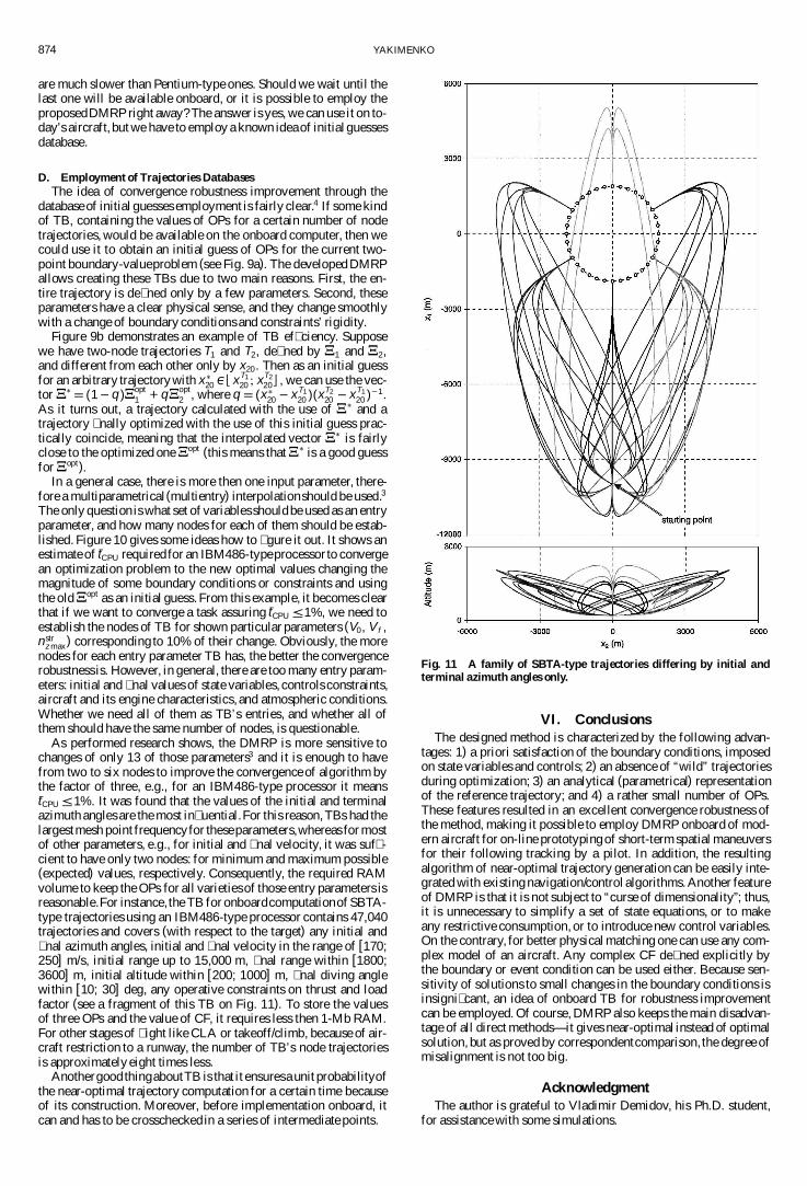
As performed research shows, the DMRP is more sensitive tochanges of only 13 of those parameters3 and it is enough to havefrom two to six nodes to improve the convergence of algorithm bythe factor of three, e.g., for an IBM486-type processor it meanstCPU ·1%. It was found that the values of the initial and terminalazimuth angles are the most in� uential.For this reason, TBs had thelargestmesh point frequencyfor theseparameters,whereas for mostof other parameters, e.g., for initial and � nal velocity, it was suf� -cient to have only two nodes: for minimum and maximum possible(expected) values, respectively. Consequently, the required RAMvolume to keep the OPs for all varietiesof those entry parameters isreasonable.For instance, the TB for onboardcomputationof SBTA-type trajectories using an IBM486-type processor contains 47,040trajectories and covers (with respect to the target) any initial and� nal azimuth angles, initial and � nal velocity in the range of [170;250] m/s, initial range up to 15,000 m, � nal range within [1800;3600] m, initial altitude within [200; 1000] m, � nal diving anglewithin [10; 30] deg, any operative constraints on thrust and loadfactor (see a fragment of this TB on Fig. 11). To store the valuesof three OPs and the value of CF, it requires less then 1-Mb RAM.For other stages of � ight like CLA or takeoff/climb, because of air-craft restriction to a runway, the number of TB’s node trajectoriesis approximately eight times less.

Anothergood thingaboutTB is that it ensuresa unit probabilityofthe near-optimal trajectory computation for a certain time becauseof its construction. Moreover, before implementation onboard, itcan and has to be crosschecked in a series of intermediate points.

Fig. 11 A family of SBTA-type trajectories differing by initial andterminal azimuth angles only.

VI. ConclusionsThe designed method is characterized by the following advan-

tages: 1) a priori satisfaction of the boundary conditions, imposedon state variables and controls; 2) an absence of “wild” trajectoriesduring optimization; 3) an analytical (parametrical) representationof the reference trajectory; and 4) a rather small number of OPs.These features resulted in an excellent convergence robustness ofthe method, making it possible to employ DMRP onboard of mod-ern aircraft for on-line prototyping of short-term spatial maneuversfor their following tracking by a pilot. In addition, the resultingalgorithm of near-optimal trajectory generation can be easily inte-grated with existing navigation/control algorithms. Another featureof DMRP is that it is not subject to “curse of dimensionality”; thus,it is unnecessary to simplify a set of state equations, or to makeany restrictive consumption, or to introduce new control variables.On the contrary, for better physical matching one can use any com-plex model of an aircraft. Any complex CF de� ned explicitly bythe boundary or event condition can be used either. Because sen-sitivity of solutions to small changes in the boundary conditions isinsigni� cant, an idea of onboard TB for robustness improvementcan be employed. Of course, DMRP also keeps the main disadvan-tage of all direct methods—it gives near-optimal instead of optimalsolution, but as proved by correspondentcomparison, the degree ofmisalignment is not too big.

AcknowledgmentThe author is grateful to Vladimir Demidov, his Ph.D. student,

for assistance with some simulations.

YAKIMENKO 875

References1Stein, K. J., “DARPA Stressing Development of Pilot’s Associate Sys-

tem; WrightLaboratoriesBroadensAdvanced TechnologiesInitiatives,” Avi-ation Week and Space Technologies, Vol. 122, No. 16, 1985, pp. 69–74,77–84.

2Yakimenko, O. A., “Shortcut-Time Spatial Trajectories Onboard Op-timization and Their Cognitive Head-Up Display Visualization for Pilot’sControl Actions During Maneuvering Support,” Proceedings of 17th IEEEInternational Congress on Instrumentation in Aerospace Simulation Facili-ties, Paci� c Grove, CA, 1997, pp. 246–256.

3Yakimenko, O. A., “Pilot Requirements to Universal Airborne Intelli-gent Pilot Decisions Support System,” Proceedings of the IEEE NationalAerospace and Electronics Conference, Dayton, OH, 1995, pp. 446–452.

4Bryson, A. E., and Ho, Y. C., Applied Optimal Control, Hemisphere,New York, 1975.

5Bellman, R., Dynamic Programming, Princeton Univ. Press, Princeton,NJ, 1957.

6Pontryagin,L. S., Boltjanskiy,V. G., Gamkrelidze, R. V., and Mishenko,E. F., The Mathematical Theory of Optimal Processes, Interscience Publish-ers, New York, 1962.

7Ewing, G. M., Calculus of Variations with Applications, W. W. Norton,New York, 1969.

8Bolza, O., Lectures on the CalculusofVariations, Univ. ofChicago Press,Chicago, 1904.

9Tonelli, L., Fondamenti di Calcolo delle Variazioni, Vols. 1 and 2,Zanichelli, Bologna, Italy, 1921 and 1923.

10Betts, J. T., “Survey of Numerical Methods for Trajectory Optimiza-tion,” Journal of Guidance, Control, and Dynamics, Vol. 21, No. 2, 1998,pp. 193–207.

11Elsgolts, L. E., Calculus of Variations, Pergamon Press, London, 1961.12Euler, L., Institutiones Calculi Integralis, Academy of Sciences, St.

Petersburg, Russia, 1768–1770.13Ritz, W., “Uber eine Neue Methode zur Losung Gewisser Variation-

sprobleme der Mathematischen Physik,” Journal fur Reine und AngewandteMathematik, No. 135, 1908, pp. 1–61.

14Krylov, N. M, “Les Methodes de Solution Approchee des Problemes dela Physique Mathematique,” Memorial des Sciences Mathematiques, fasci-cule 49, Gauntier-Villars et Cie., Paris, 1931.

15Galerkin, B. G., “Series Development for Some Cases of Elastic Equi-librium of the Rods and Plates,” Bulletin of Engineers and Technicians,Petrograd, Vol. 19, 1915, pp. 897–908 (in Russian).

16Kantorovich, L. V., and Krylov, V. I., Approximate Methods of HigherAnalysis, Interscience Publishers, Inc., New York, 1958.

17Mikhlin,S. G., Direct Methodsof MathematicalPhysics, Gostekhizdat,Moscow, 1950 (in Russian).

18Taranenko, V. T., Experience of Employment the Ritz’s, Poincare’s, andLyapunov’s Methodsfor Solving the Problems of FlightDynamics, Air ForceEngineering Academy Prof. N. Zhukovskiy Press, Moscow, 1968 (in Rus-sian).

19Staugler, A. J., Chart, D. A., and Melton, R. G., “Reversed-Series So-lution to the Universal Kepler Equation,” Journal of Guidance, Control, andDynamics, Vol. 20, No. 6, 1997, pp. 1276, 1277.

20Taranenko, V. T., and Momdzhi, V. G., Direct Variational Methodin Boundary Value Problems of Flight Dynamics, Mashinostroenie Press,Moscow, 1968 (in Russian).

21Blagodarniy,M. A., “Direct Method for N-point Boundary Value Prob-lems,” Zhukovskiy Air Force Engineering Academy Press—Flight DynamicsIssue (Air Force Engineering Academy Press), Moscow, 1989, pp. 3–17 (inRussian).

22Akulov, V. Yu., and Schisljonok, A. M., “Foundation of a New Di-rect Method for Trajectories Optimization,” Air Force Engineering AcademyPress, Moscow, 1991, pp. 1–11 (in Russian).

23Neljubov, A. I., “Mathematical Methods of Calculation of Combat,Takeoff/Climb, and Landing Approach Maneuvers for the Aircraft with2-D Thrust Vectoring. Flight Characteristics and Combat Maneuvering ofManned Vehicles,” Air Force Engineering Academy Press, Moscow, 1986(in Russian).

24Hargraves, C. R., and Paris, S. W., “Direct Trajectory Optimization Us-ing NonlinearProgrammingand Collocation,”JournalofGuidance,Control,and Dynamics, Vol. 10, No. 4, 1987, pp. 338–342.

25VonStryk,O., and Bulirsch, R., “Direct and IndirectMethodsforTrajec-tory Optimization,” Annals of Operations Research, Vol. 37, 1992, pp. 357–

373.26Enright, P. J., and Convay, B. A., “Discrete Approximations to Opti-

mal Trajectories Using Direct Transcription and Nonlinear Programming,”Journal of Guidance, Control, and Dynamics, Vol. 15, No. 5, 1992, pp. 994–

1002.27Herman, A. L., and Convay, B. A., “Direct Optimization Using Collo-

cation Based on High-Order Gauss-Lobatto Quadrature Rules,” Journal ofGuidance, Control, and Dynamics, Vol. 19, No. 3, 1996, pp. 592–599.

28Betts, J. T., “Path-Constrained Trajectory Optimization Using SparseSequential Quadratic Programming,” Journal of Guidance, Control, andDynamics, Vol. 16, No. 1, 1993, pp. 59–68.

29Calise, A. J., and Leung, M. S. K., “Hybrid Approach to Solution ofOptimal Control Problems,” Journal of Guidance, Control, and Dynamics,Vol. 17, No. 5, 1994, pp. 966–974.

30Hull, D. G., “Conversion of Optimal Control Problems into Parame-ter Optimization Problems,” Journal of Guidance, Control, and Dynamics,Vol. 20, No. 1, 1997, pp. 57–60.

31Seywald, H., “Trajectory Optimization Based on Differential Inclu-sions,” Journal of Guidance, Control, and Dynamics, Vol. 17, No. 3, 1994,pp. 480–487.

32Kumar, R., and Seywald, H., “Dense-Sparse Discretization for Opti-mization and Real-Time Guidance,” Journal of Guidance, Control, and Dy-namics, Vol. 19, No. 2, 1996, pp. 501–503.

33Kumar, R., and Seywald, H., “Should Controls Be Eliminated WhileSolving Optimal Control Problems via Direct Methods?” Journal of Guid-ance, Control, and Dynamics, Vol. 19, No. 2, 1996, pp. 418–423.

34Convay, B. A., and Larson, K. M., “Collocation Versus DifferentialInclusion in Direct Optimization,” Journal of Guidance, Control, and Dy-namics, Vol. 21, No. 5, 1998, pp. 780–785.

35Lu, P., “Inverse Dynamics Approach to Trajectory Optimization for anAerospace Plane,” Journal of Guidance, Control, and Dynamics, Vol. 16,No. 4, 1993, pp. 726–732.

36Lu, P., and Asif Khan, M., “Nonsmooth Trajectory Optimization: AnApproach Using Continuous Simulated Annealing,” Journal of Guidance,Control, and Dynamics, Vol. 17, No. 4, 1994, pp. 685–691.

37Sentoh,E., and Bryson,A. E., “Inverse and Optimal Control for DesiredOutputs,” Journalof Guidance,Control, andDynamics, Vol. 15, No. 3, 1992,pp. 687–691.

38Lane, S. H., and Stengel, R. F., “FlightControlDesign Using NonlinearInverse Dynamics,” Automatica, Vol. 24, No. 4, 1988, pp. 471–483.

39Hooke, R., and Jeeves, T. A., “ ‘Direct Search’ Solution of Numericaland Statistical Problems,” Journal of the Association for Computing Ma-chinery, Vol. 8, No. 2, 1961, pp. 212–229.

40Nelder, J. A., and Mead, R., “A Simplex Method for Function Mini-mization,” The Computer Journal, Vol. 8, No. 7, 1965, pp. 308–313.

41Strongin, R. G., and Markin, D. L., “Minimization of MultiextremalFunctionsUnderNonconvexConstraints,” Cybernetics, Vol. 22, No. 4, 1987,pp. 486–493.

42Dobrokhodov,V. N., and Yakimenko, O. A., “Synthesis of TrajectorialControl Algorithms at the Stage of Rendezvous of an Airplane with a Ma-neuveringObject,” JournalofComputerandSystems Sciences International,Vol. 38, No. 2, 1999, pp. 262–277.