Direct estimate for positive linear operators in polynomial weighted spaces
14
Journal of Approximation Theory 162 (2010) 1495–1508 www.elsevier.com/locate/jat Direct estimate for positive linear operators in polynomial weighted spaces Jorge Bustamante a , Jos´ e M. Quesada b,* , Lorena Morales de la Cruz a a Fac. Ciencias F´ ısico Matem´ aticas, B. Universidad Aut´ onoma de Puebla, Av. San Claudio y R´ ıo Verde, San Manuel, 62570 Puebla, Puebla, Mexico b Escuela Polit´ ecnica Superior, University of Ja´ en, 23071-Ja´ en, Spain Received 5 October 2009; accepted 1 April 2010 Available online 10 April 2010 Communicated by Zeev Ditzian Abstract We present direct theorems for some sequences of positive linear operators in weighted spaces. The results, given in terms of some Ditzian–Totik moduli of smoothness, include estimations in norms and Becker type estimations. c 2010 Elsevier Inc. All rights reserved. Keywords: Positive linear operators; Weighted approximation; Direct a theorems; Baskakov-type operators; Sz´ asz–Mirakyan-type operators 1. Introduction and notations For n ≥ 1 and f ∈ C [0, 1], the Bernstein operator B n is defined by B n ( f , x ) = n X k =0 n k x k (1 - x ) n-k f k n , x ∈[0, 1]. In [7], Ditzian proved that for α ∈[0, 1/2] and ϕ(x ) = (x (1 - x )) α there exists a constant C ϕ , such that, for f ∈ C [0, 1] and x ∈ (0, 1), * Corresponding author. E-mail address: [email protected] (J.M. Quesada). 0021-9045/$ - see front matter c 2010 Elsevier Inc. All rights reserved. doi:10.1016/j.jat.2010.04.001
-
Upload
jorge-bustamante -
Category
Documents
-
view
214 -
download
0
Transcript of Direct estimate for positive linear operators in polynomial weighted spaces

Journal of Approximation Theory 162 (2010) 1495–1508www.elsevier.com/locate/jat
Direct estimate for positive linear operators inpolynomial weighted spaces
Jorge Bustamantea, Jose M. Quesadab,∗, Lorena Morales de la Cruza
a Fac. Ciencias Fısico Matematicas, B. Universidad Autonoma de Puebla, Av. San Claudio y Rıo Verde, San Manuel,62570 Puebla, Puebla, Mexico
b Escuela Politecnica Superior, University of Jaen, 23071-Jaen, Spain
Received 5 October 2009; accepted 1 April 2010Available online 10 April 2010
Communicated by Zeev Ditzian
Abstract
We present direct theorems for some sequences of positive linear operators in weighted spaces. Theresults, given in terms of some Ditzian–Totik moduli of smoothness, include estimations in norms andBecker type estimations.c© 2010 Elsevier Inc. All rights reserved.
Keywords: Positive linear operators; Weighted approximation; Direct a theorems; Baskakov-type operators;Szasz–Mirakyan-type operators
1. Introduction and notations
For n ≥ 1 and f ∈ C[0, 1], the Bernstein operator Bn is defined by
Bn( f, x) =n∑
k=0
(n
k
)xk(1− x)n−k f
(k
n
), x ∈ [0, 1].
In [7], Ditzian proved that for α ∈ [0, 1/2] and ϕ(x) = (x(1 − x))α there exists a constantCϕ , such that, for f ∈ C[0, 1] and x ∈ (0, 1),
∗ Corresponding author.E-mail address: [email protected] (J.M. Quesada).
0021-9045/$ - see front matter c© 2010 Elsevier Inc. All rights reserved.doi:10.1016/j.jat.2010.04.001

1496 J. Bustamante et al. / Journal of Approximation Theory 162 (2010) 1495–1508
| f (x)− Bn( f, x)| ≤ Cϕω2ϕ
(f,
√x(1− x)√
nϕ(x)
), (1)
where
ω2ϕ( f, h) = sup
0≤s≤hsup
x∈I (ϕ,s)|∆2
sϕ(x) f (x)|, (2)
I (ϕ, s) = {x ∈ [0, 1] : 0 ≤ x − sϕ(x) < x + sϕ(x) ≤ 1} and ∆2u f (x) := f (x − u)− 2 f (x)+
f (x+u) is the usual symmetric difference of order 2 of the function f at x with step u. This resultunifies the classical estimate for α = 0 with the norm estimate for α = 1/2 (Ditzian–Totik, [8],p. 117). An extension was given by Felten in [9]. He proved the inequality
| f (x)− Bn( f, x)| ≤ Cω2φ
(f,
√x(1− x)√
nφ(x)
), (3)
where φ : [0, 1] → R is an admissible step-weight function of the Ditzian Totik modulus(see [8]) such that φ2 is a concave function.
In [10] Finta presents several condition for a sequence of positive linear operators Ln :
C[0, 1] → C[0, 1] in order to obtain a local direct approximation theorem similar to (3).In 1978 Becker [4] studied Baskakov and Szasz–Mirakyan operators in polynomial weighted
spaces. After that, several papers have appeared devoted to consider sequences of positive linearoperators in polynomial weighted spaces. As it was pointed out in [5], it is not clear what moduliof smoothness should be used to measure the rate of convergence on these spaces.
In order to present the main results of this paper we need some notation.Throughout the paper m ∈ N is fixed and we consider the weight
ρ(x) = ρm(x) = (1+ x)−m, x ∈ I = [0,∞). (4)
Moreover C(I )(Cb(I )) is the family of all (bounded) continuous functions defined on I .Since m will be fixed we omit the parameter m in the notations. The polynomial weighted
space associated to (4) is defined by
Cρ(I ) = { f ∈ C(I ) : ‖ f ‖ρ <∞}
where
‖ f ‖ρ = supx≥0
ρ(x)| f (x)|.
We remark that some authors use the weight ρ1(x) = (1+xm)−1. It is clear that the associatedweighted spaces are the same with equivalent norms.
For a ∈ N0, b > 0 and c ≥ 0 we denote
ϕ(x) =√(1+ ax)(bx + c).
For λ ∈ [0, 1], r = 1, 2 and f ∈ Cρ(I ), we consider the K -functional
Kr,ϕλ( f, t)ρ = inf {‖ f − g‖ρ + tr‖ϕλ r g(r)‖ρ, g ∈ W∞r,λ(ϕ)}, (5)
where W∞r,λ(ϕ) consists of all functions g ∈ Cρ[0,∞) such that g(r−1) is absolutely continuouson [0,∞) and ‖ϕλ r g(r)‖ρ <∞.
Here and below the norm ‖ϕλ r g(r)‖ρ is considered in L∞(0,∞).
J. Bustamante et al. / Journal of Approximation Theory 162 (2010) 1495–1508 1497
In Theorem 1 we will present some conditions, for a sequence of positive linear operators{Ln}, which guarantee that the error ρ(x)| f (x) − Ln( f, x)| can be estimated in terms of theK -functional (5). In particular we are looking for estimations similar to (3). That is
ρ(x)| f (x)− Ln( f, x)| ≤ C Kr,ϕλ( f,√αnϕ
1−λ(x))ρ, x ≥ 0, (6)
where we take r = 1 if each Ln reproduces constant functions and r = 2 if each Ln reproduceslinear functions.
In Theorem 2 we show that, if we have on hand a good representation for the functionsLn(tk, x), then the conditions of Theorem 1 hold.
Usually, when one tries to obtain an estimation like (1), a characterization of the modulusof smoothness in terms of an appropriated K -functional is needed. This means a system ofinequalities of the form
C1ω2ϕλ( f, t)ρ ≤ K2,ϕλ( f, t)ρ ≤ C2 ω
2ϕλ( f, t)ρ, (7)
where the modulus is defined in (8). Of course, in this paper we only need the second inequality.For weighted moduli of smoothness the main reference for such a characterization is themonograph of Ditzian and Totik, [8]. In [8] all the inequalities like (7) are proved for t ∈ (0, t0],where the number t0 < 1 depends on the weight ϕ. On the other hand, for an unbounded intervaland weight function like ϕ(x) =
√x(1+ a x), the argument of the K -functional in (6) is not
bounded (for λ 6= 1). We remark that some authors have used the result of Ditzian and Totik forall values of t , but we have not found any proof for such a characterization.
In the most important cases (λ = 0 (pointwise Becker-type estimate) and λ = 1 (estimate innorm)), we can use Theorems 1 and 2 to obtain estimates in terms of moduli of smoothness. Thiswill be accomplished in Theorem 3. In particular, for estimations in norm we use a weightedmodulus defined, for f ∈ Cρ(I ), by
ω2ϕ( f, t)ρ = sup
h∈(0,t]sup
x∈I (ϕ,h)|ρ(x)∆2
hϕ(x) f (x)| (8)
where I (ϕ, h) = {x > 0 : hϕ(x) ≤ x}. If we denote by Cρ,∞ the set of all continuousfunctions on [0,∞) such that ρ(x) f (x) has finite limit as x → ∞, then it can be proved thatlimt→0+ ω
2ϕλ( f, t)ρ = 0, whenever f ∈ Cρ,∞[0,∞). For pointwise estimates we provide results
in terms of the moduli of continuity analogous to the ones used by Becker in [4].In the last section we give several examples of applications of Theorems 1 and 2.
2. The main results
Proposition 1. For m ∈ N, set ρ(x) = (1+ x)−m . For a ∈ N0 and b, c real numbers with b > 0and c ≥ 0, set θ(x) = (1 + a x)(b x + c). Then, for all α, γ such that 1 + α > γ and m ≥ γ ,there exists a constant C = C(a, α, γ ) such that, for all x, t ∈ [0,∞),∣∣∣∣∫ t
x
|t − u|α
θ(u)γ ρ(u)du
∣∣∣∣ ≤ C|t − x |α+1
θ(x)γ
(1
ρ(x)+
1ρ(t)
). (9)
Proof. First we estimate the integral for the case a > 0. Taking into account that 1 + x ≤1+ ax ≤ a(1+ x), we obtain, for t ≤ x ,∣∣∣∣∫ t
x
|t − u|αdu
θ(u)γ ρ(u)
∣∣∣∣ = ∫ x
t
(u − t)α(1+ u)m
(bu + c)γ (1+ au)γdu ≤
∫ x
t
(u − t)α(1+ u)m−γ
(bu + c)γdu

1498 J. Bustamante et al. / Journal of Approximation Theory 162 (2010) 1495–1508
≤ (1+ x)m−γ∫ x
t
(u − t)α
(bu + c)γdu
=(x − t)1+α(1+ x)m
(1+ x)γ
∫ 1
0
ταdτ(c + bτ x + b(1− τ)t)γ
≤(x − t)1+α(1+ x)m
(1+ x)γ (bx + c)γ
∫ 1
0τα−γ dτ ≤
C(x − t)1+α
θ(x)γ ρ(x),
with C = aγ /(1+ α − γ ). Moreover, if x < t ,∣∣∣∣∫ t
x
|t − u|αdu
θ(u)γ ρ(u)
∣∣∣∣ = ∫ t
x
(t − u)α
θ(u)γ ρ(u)du ≤
1θ(x)γ ρ(t)
∫ t
x(t − u)du
=1
1+ α(t − x)1+α
θ(x)γ ρ(t)≤ C
(t − x)1+α
θ(x)λρ(t).
For a = 0 we obtain analogous inequalities with C = 1/(1+ α − λ). �
Theorem 1. Fix a positive integer m and set ρ(x) = (1 + x)−m . For a ∈ N0 and b, c realnumbers with b > 0 and c ≥ 0, set ϕ(x) =
√(1+ ax)(bx + c).
Let {Ln}, Ln : Cρ(I ) → C(I ), be a sequence of positive linear operators satisfying thefollowing conditions:
(i) Ln(e0) = e0.(ii) There exist a constant C1 and a sequence {αn} such that
Ln((t − x)2, x) ≤ C1 αn ϕ2(x).
(iii) There exists a constant C2 = C2(m) such that, for each n ∈ N,
Ln((1+ t)m, x) ≤ C2(1+ x)m, x ≥ 0.
(iv) There exists a constant C3 = C3(m) such that, for every n ∈ N,
ρ(x)Ln((t − x)2/ρ(t), x) ≤ C3 αn ϕ2(x), x ≥ 0.
Then, for λ ∈ [0, 1], there exists a constant C4 = C4(m, λ) such that for any f ∈ Cρ(I ),x ∈ I and n ∈ N, one has
ρ(x)| f (x)− Ln( f, x)| ≤ C4 K1,ϕλ( f,√αnϕ
1−λ(x))ρ, x ≥ 0. (10)
where K1,ϕλ( f, t)ρ is the K -functional defined in (5) with r = 1.If, in addition, Ln(e1) = e1, then there exists a constant C5 = C5(m, λ) such that
ρ(x)| f (x)− Ln( f, x)| ≤ C5 K2,ϕλ( f,√αnϕ
1−λ(x))ρ, x ≥ 0. (11)
where K2,ϕλ( f, t)ρ is the K -functional defined in (5) with r = 2.
Proof. Fix f ∈ Cρ(I ) and x ≥ 0. From condition (iii) one has
ρ(x)|Ln( f, x)| ≤ ‖ f ‖ρ ρ(x) Ln(1/ρ, x) ≤ C2‖ f ‖ρ .
Therefore
‖Ln( f )‖ρ ≤ C2‖ f ‖ρ . (12)

J. Bustamante et al. / Journal of Approximation Theory 162 (2010) 1495–1508 1499
For an arbitrary g ∈ W∞1,λ(ϕ), we use the representation
g(t) = g(x)+∫ t
xg′(u)du = g(x)+ M(g, t, x),
to obtain
ρ(x)|( f (x)− Ln( f, x))| ≤ (1+ C2)‖ f − g‖ρ + ρ(x)|g(x)− Ln(g, x)|
≤ (1+ C2)‖ f − g‖ρ + ρ(x)Ln (|M(g, t, x)|, x)
≤ (1+ C2)‖ f − g‖ρ + ρ(x)‖ϕλg′‖ρLn
(∣∣∣∣∫ t
x
du
ϕλ(u)ρ(u)
∣∣∣∣ , x
). (13)
From Proposition 1 with α = 0, γ = λ/2 and conditions (ii) and (iv), we obtain
ρ(x)Ln
(∣∣∣∣∫ t
x
du
ϕλ(u)ρ(u)
∣∣∣∣ , x
)≤ C
(1
ϕλ(x)Ln(|t − x |, x)+
ρ(x)
ϕλ(x)Ln(|t − x |/ρ(t), x)
)≤ C
(1
ϕλ(x)
√Ln((t − x)2, x)+
ρ(x)
ϕλ(x)
√Ln(1/ρ(t), x)Ln((t − x)2/ρ(t), x)
)≤ C
( √C1
ϕλ(x)
√αnϕ(x)+
ρ(x)
ϕλ(x)
√C2/ρ(x)
√C3αnϕ2(x)/ρ(x)
)= C√αnϕ
1−λ(x),
where C = C(√
C1 +√
C2 C3). Finally, (13) yields
ρ(x)| f (x)− Ln( f, x)| ≤ (1+ C2)‖ f − g‖ρ + C√αnϕ
1−λ(x)‖ϕλg′‖ρ .
Since g ∈ W∞1,λ(ϕ) is arbitrary, one has
ρ(x)| f (x)− Ln( f, x)| ≤ C4 K1,ϕλ
(f,√αnϕ
1−λ(x))ρ,
where C4 = max{(1+ C2), C
}.
Assume that, in addition, Ln(e1) = e1. For an arbitrary g ∈ W∞2,λ(ϕ), using the representation
g(t) = g(x)+ g′(x)(t − x)+∫ t
xg′′(u)(t − u)du = g(x)+ g′(x)(t − x)+ N (g, t, x)
and (12), we have
ρ(x)|( f (x)− Ln( f, x))| ≤ (1+ C2)‖ f − g‖ρ + ρ(x)|(g(x)− Ln(g, x))|
≤ (1+ C2)‖ f − g‖ρ + ρ(x)Ln (|N (g, t, x)|, x)
≤ (1+ C2)‖ f − g‖ρ + ρ(x)‖ϕ2λg′′‖ρLn
(∣∣∣∣∫ t
x
|t − u|
ϕ2λ(u)ρ(u)du
∣∣∣∣ , x
). (14)
From Proposition 1 with α = 1, γ = λ, b = 1, c = 0, and conditions (ii) and (iv), we obtain
ρ(x)Ln
(∣∣∣∣∫ t
x
|t − u|
ϕ2λ(u)ρ(u)
∣∣∣∣ du, x
)≤ C
(1
ϕ2λ(x)Ln((t − x)2, x)+
ρ(x)
ϕ2λ(x)Ln((t − x)2/ρ(t), x)
)≤ C αn ϕ
2(1−λ)(x),

1500 J. Bustamante et al. / Journal of Approximation Theory 162 (2010) 1495–1508
where C = C(C1 + C3). Finally, (14) yields
ρ(x)| f (x)− Ln( f, x)| ≤ (1+ C2)‖ f − g‖ρ + C αn ϕ2(1−λ)(x)‖ϕ2λg′′‖ρ .
Since g ∈ W∞2,λ(ϕ) is arbitrary, one has
ρ(x)| f (x)− Ln( f, x)| ≤ C5 K2,ϕλ
(f,√αn ϕ
(1−λ)(x))ρ,
where C5 = max{(1+ C2), C}. �
Remark 1. When αn → 0 (as n → ∞) and f ∈ Cρ,∞(I ), Theorem 1 provides an estimationfor the rate of convergence.
In some case conditions (i)–(iv) in Theorem 1 can be deduced from some identities associatedto the operators.
Theorem 2. Fix a positive integer m and set ρ(x) = (1+ x)−m . Let Lm(I ) be a linear subspaceof C(I ) containing the functions ek(t) = tk , 0 ≤ k ≤ m + 2 and {Ln}, Ln : Lm(I )→ C(I ), bea sequence of positive linear operators. Moreover, assume that for every k ∈ {0, 1, . . . ,m + 2}there exist real numbers {ak, j }
kj=0 with ak,k = 1 such that, for each n ∈ N, one has
Ln(tk, x) =
k∑j=0
ak, jx j
nk− j , x ≥ 0. (15)
Then, (10) holds with αn = 1/n and ϕ(x) =√
1+ x. Moreover, if ak,0 = 0 for 1 ≤ k ≤ m + 2,then (11) holds with αn = 1/n and ϕ(x) =
√x.
Proof. We will prove that conditions (i)–(iv) in Theorem 1 hold.From (15) with k = 0 we obtain L(e0) = e0 and then (i) holds.Let us denote Cm = max{|ak, j | : 0 ≤ j ≤ k ≤ m + 2}. From the representation (15) we
obtain
Ln((1+ t)m, x) =m∑
k=0
(m
k
)Ln(t
k, x) = 1+m∑
k=1
(m
k
) k∑j=0
ak, jx j
nk− j
≤ 1+ Cm
m∑j=0
x jm∑
k= j
(m
k
)≤ 1+ 2mCm(1+ x)m ≤ C2(1+ x)m,
where C2 = 1+ 2mCm , and (iii) holds.Using again (15), for 0 ≤ k ≤ m, we have
Ln((t − x)2tk, x) = Ln(tk+2, x)− 2x Ln(t
k+1, x)+ x2Ln(tk, x)
=ak+2,0
nk+2 +ak+2,1 − 2ak+1,0
nk+1 x +k+2∑j=2
ak+2, j − 2ak+1, j−1 + ak, j−2
nk+2− jx j
=ak+2,0
nk+2 +ak+2,1 − 2ak+1,0
nk+1 x +k+1∑j=2
ak+2, j − 2ak+1, j−1 + ak, j−2
nk+2− jx j ,
where in the case k = 0 the last term is omitted. From this we obtain
Ln((t − x)2tk, x) ≤ 4Cm1+ x
n(1+ x)k (16)

J. Bustamante et al. / Journal of Approximation Theory 162 (2010) 1495–1508 1501
and in the case ak,0 = 0 (k > 0)
Ln((t − x)2tk, x) ≤ 4Cmx
n(1+ x)k . (17)
Then, from (16) we conclude that
Ln((t − x)2(1+ t)m, x) =m∑
k=0
(m
k
)Ln((t − x)2tk, x) ≤ C3
1+ x
n(1+ x)m,
where C3 = 2m+2Cm , and then (iv) holds with αn = 1/n and ϕ(x) =√
1+ x .Analogously, in the case ak,0 = 0, from (17) we have
Ln((t − x)2(1+ t)m, x) ≤ C3x
n(1+ x)m,
and (iv) holds with αn = 1/n and ϕ(x) =√
x .Notice that, particularizing (16) and (17) for k = 0, we deduce that (ii) also holds with
αn = 1/n and ϕ(x) =√
1+ x , in the general case, and with αn = 1/n and ϕ(x) =√
x , in thecase a1,0 = a2,0 = 0.
Finally, from (15) it is immediate that if a1,0 = 0, then Ln(t, x) = x . �
Let us present some results in terms of moduli of smoothness. Following [4], for f ∈ Cρ(I )and h > 0 we set
ω2( f, t)ρ = sup0<h≤t
supx≥0
ρ(x) | f (x + 2h)− 2 f (x + h)+ f (x) | . (18)
Theorem 3. Assume that the conditions of Theorem 1 hold with ϕ(x) =√
x(1+ ax) andLn(e1) = e1. Then
(i) There exists a constant C such that, for any f ∈ Cρ(I ) and n ∈ N such that αn ≤
1/(2√
2+ a),
‖ f − Ln( f )‖ρ ≤ Cω2ϕ( f,√αn)ρ, (19)
where ω2ϕ( f, t)ρ is the modulus in (8), with λ = 1.
(ii) There exists a constant C such that, for any f ∈ Cρ(I ) and n ∈ N,
ρ(x)| f (x)− Ln( f, x)| ≤ Cω2 ( f,√αnϕ(x)
)ρ, x ≥ 0 (20)
where ω2( f, t)ρ is the modulus defined in (18).
Proof. (i) The result is derived from (11) (with λ = 1), if we are able to verify (7). From [8]we know that (7) holds for t ∈ (0, t0], where t0 is chosen as follows (see [8], p. 16–17). Fix anumber A such that ϕ(x) ≤ A
√x , for 0 ≤ x ≤ 1/2 and, for any t > 0, set t∗ = (2At)2. Then,
t0 is taken in such a way that, for 0 < h ≤ t < t0 and x > t∗, one has
x
2≤ x − hϕ(x). (21)
Thus, we can take A =√
1+ a/2 and t∗ = 2(2+ a)t2. Since (21) is equivalent to
4h2
1− 4ah2 ≤ x

1502 J. Bustamante et al. / Journal of Approximation Theory 162 (2010) 1495–1508
(assuming 4ah2 < 1), one needs
4t2
1− 4at2 ≤ x, for t∗ < x .
But the inequality
4t2
1− 4at2 ≤ t∗
is just equivalent to
t2≤
14(2+ a)
.
Thus we can chose t0 = 1/(2√
2+ a ).(ii) In this case the result is also derived from (11) (with λ = 0), since from equation (21)
in [4] we know that, for any h > 0,
K2,ϕ0( f, h2)ρ ≤ 10ω2( f, h)ρ . �
A similar result holds in the case when the operators reproduce only constant functions. Weomit the proof.
Theorem 4. Assume that the conditions of Theorem 1 hold with ϕ(x) =√
x(1+ ax) (withoutassuming Ln(e1) = e1). Then
(i) There exists a constant C such that, for any f ∈ Cρ(I ) and n ∈ N such that αn ≤
1/(2√
2+ a),
‖ f − Ln( f )‖ρ ≤ Cω1ϕ( f,√αn)ρ, (22)
where
ω1ϕ( f, t)ρ = sup
h∈(0,t]sup
2x≥hϕ(x)
∣∣∣∣ρ(x)( f
(x +
h
2ϕ(x)
)− f
(x −
h
2ϕ(x)
))∣∣∣∣(ii) There exists a constant C such that, for any f ∈ Cρ(I ) and n ∈ N,
ρ(x)| f (x)− Ln( f, x)| ≤ Cω1 ( f,√αnϕ(x)
)ρ, x ≥ 0. (23)
where
ω1( f, t)ρ = sup0<h≤t
supx≥0
ρ(x)| f (x + h)− f (x)|.
3. Applications
As a first example, let us consider a sequence of Baskakov-type operators.
Theorem 5. Fix a positive integer m and set ρ(x) = (1 + x)−m . Moreover, fix a ∈ N and setφn,a(x) = (1 + ax)−n/a . Let {Ln,a}, Ln,a : Cρ(I ) → C(I ), be the sequence of positive linearoperators defined by
Ln,a( f, x) =∞∑
k=1
f
(k
n
)(−1)k
φ(k)n,a(x)xk
k!, x ≥ 0. (24)
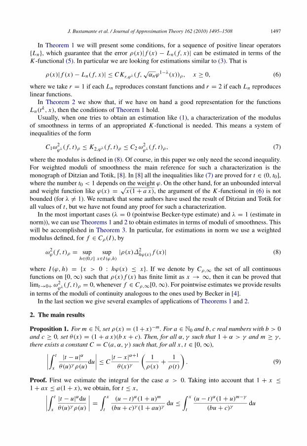
J. Bustamante et al. / Journal of Approximation Theory 162 (2010) 1495–1508 1503
Then, there exists a constant C such that, for any f ∈ Cρ(I ), x ∈ I and n ∈ N, one has
ρ(x)| f (x)− Ln,a( f, x)| ≤ Cω2
(f,
√x(1+ ax)
n
)ρ
, (25)
where ω2( f, t)ρ is the modulus defined in (8) with λ = 0.Moreover, for n ≥ 2
√2+ a, one has
‖ f − Ln,a( f )‖ρ ≤ Cω2ϕ( f, 1/
√n)ρ,
where ϕ(x) =√
x(1+ ax).
Proof. These operators satisfy conditions (i) and (ii) in Theorem 1 with αn = 1/n andϕ(x) =
√x(1+ ax). Moreover, Ln(e1) = e1. That the sequence {Ln,a} satisfy conditions (iii)
and (iv) in Theorem 1 can be proved as in [4], where the case a = 1 was considered.The result also follows from Theorem 2, because the equality (15) with ak,0 = 0 can be proved
by using the ideas in Lemma 3 of [4]. �
As a second example let us consider the following sequence of Szasz–Mirakyan typeoperators.
Theorem 6. Fix c ∈ R (c ≥ 0), a positive integer m, λ ∈ [0, 1] and set ρ(x) = (1+ x)−m . Let{Sn,c}, Sn,c : Cρ(I )→ C(I ), be the sequence of positive linear operators defined by
Sn,c( f, x) = e−(n+c)x∞∑
k=0
(n + c)k xk
k!f
(k
n + c
), x ≥ 0.
Then there exists a constant C such that, for any f ∈ Cρ(I ), x ∈ I and n ∈ N one has
ρ(x)| f (x)− Sn,c( f, x)| ≤ Cω2( f,√
x/(n + c))ρ, (26)
where ω2( f, t)ρ is the modulus defined in (8) with λ = 0.Moreover, for n ≥ 3, one has
‖ f − Sn,c( f )‖ρ ≤ Cω2ϕ( f, 1/
√n + c)ρ,
where ϕ(x) =√
x and ω2ϕ( f, t)ρ is the modulus defined in (8) with λ = 1.
Proof. In this case (i) and (ii) in Theorem 1 hold with ϕ(x) =√
x and αn = 1/(n+c). Moreover,Ln(e1) = e1. That the other conditions are satisfied can be proved with an argument similar tothe one given for the Baskakov type operators presented above. �
Remark 2. For each n ∈ N, the operator Sn,0 (c = 0) is just the so called Szasz–Mirakyanoperator. For these operators Becker [4] proved the inequality (26). Also Becker obtained asimilar estimation as in (25) for the Baskakov operators.
As a third example let us consider the Phillips operators.
Theorem 7. Fix a positive integer m, λ ∈ [0, 1] and set ρ(x) = (1 + x)−m . Let {Pn},Pn : Cρ(I )→ C(I ), be the sequence of positive linear operators defined by
Pn( f, x) = e−nx f (0)+ n∞∑
k=1
sn,k(x)∫∞
0sn,k−1(t) f (t)dt,

1504 J. Bustamante et al. / Journal of Approximation Theory 162 (2010) 1495–1508
where
sn,k(x) = e−nk (nx)k
k!.
There exists a constant C such that, for any f ∈ Cρ(I ), x ∈ I and n ∈ N one has
ρ(x)| f (x)− Pn( f, x)| ≤ Cω2( f,√
2x/n)ρ,
where ω2( f, t)ρ is the modulus defined in (8) with λ = 0.Moreover, for n ≥ 6, one has
‖ f − Pn( f )‖ρ ≤ Cω2ϕ( f,
√2/n)ρ,
where ϕ(x) =√
x and ω2ϕ( f, t)ρ is the modulus defined in (8) with λ = 1.
Proof. We will verify all the conditions in Theorem 2. A direct calculus shows that
Pn( f, 0) = 0, Pn(1, x) = 1, Pn(t, x) = x and Pn((t − x)2, x) =2x
n.
Let the numbers {ar, j } j∈Z be defined as follows: ar, j = 0 if j > r or j ≤ 0, a1,1 = 1, a2,1 = 2,a2,2 = 1 and
ar+1, j = (r + j)ar, j + ar, j−1, for 1 ≤ j ≤ r + 1.
We will prove by induction on r that, for n, r ∈ N one has
Pn(tr , x) =
r∑j=1
ar, jx j
nr− j .
Since Pn(t, x) = x , the assertion holds for r = 1.Taking into account that xs′n,k(x) = (k − nx)sn,k(x), for r ≥ 1, one has
x P ′n(tr , x) = nx
∞∑k=1
s′n,k(x)∫∞
0sn,k−1(t)t
r dt = n∞∑
k=1
(k − nx)sn,k(x)∫∞
0sn,k−1(t)t
r dt
= n∞∑
k=1
sn,k(x)∫∞
0(k − 1− nt + n(t − x)+ 1)sn,k−1(t)t
r dt
= n∞∑
k=1
sn,k(x)∫∞
0s′n,k−1(t)t
r+1dt + n2∞∑
k=1
sn,k(x)∫∞
0sn,k−1(t)t
r+1dt
+ n(1− nx)∞∑
k=1
sn,k(x)∫∞
0sn,k−1(t)t
r dt
= −n(r + 1)∞∑
k=1
sn,k(x)∫∞
0sn,k−1(t)t
r dt + n Pn(tr+1, x)+ (1− nx)Pn(t
r , x).
Therefore
Pn(tr+1, x) =
x
nP ′n(t
r , x)+r + nx
nPn(t
r , x). (27)

J. Bustamante et al. / Journal of Approximation Theory 162 (2010) 1495–1508 1505
Now, assume that the assertion is true for some r ≥ 1. Then from (27) we obtain
Pn(tr+1, x) =
x
n
r∑j=1
ar, jj x j−1
nr− j +r + nx
n
r∑j=1
ar, jx j
nr− j
=
r+1∑j=1
( j + r)ar, jx j
nr+1− j+
r+1∑j=1
ar, j−1x j
nr+1− j(ar,r+1 = ar,0 = 0)
=
r+1∑j=1
ar+1, jx j
nr+1− j. �
As another example, we consider some operators studied by Abel and Ivan in [2]. Let E bethe class of all functions of exponential type on [0,∞). That is, f ∈ E if there are constants Kand A such that, | f (x)| ≤ K eAx , x ≥ 0.
For d > 0 fixed, set
Sn,d( f, x) =∞∑
k=0
pn,k,d(x) f
(k
n
), (28)
where
pn,k,d(x) =
(d
1+ d
)ndx (ndx + k − 1k
)(1+ d)−k,
(ndx − 1
0
)= 1
and (ndx + k − 1
k
)=(ndx)(ndx + 1) · · · (ndx + k − 1)
k!.
Notice that, if | f (x)| ≤ K eAx and n > A/ log(1+d), then the series given in (28) converges.Thus, for n > 1/ log(1 + d), the operator (28) is well defined for every function f withpolynomial growth.
In the special case d = 1 we obtain the operators
Ln( f, x) = 2−nx∞∑
k=0
(nx + k − 1
k
)2−k f
(k
n
)introduced by Lupas [13]. In [3], Agratini investigated the convergence of these Lupas operators,but only for compact subset of [0,∞). We remark that Abel and Ivan [2] also provided estimateof the rate of convergence (in terms of the first usual modulus of continuity), when operators Sn,dare applied to bounded function.
Theorem 8. Fix d > 0, a positive integer m, λ ∈ [0, 1] and set ρ(x) = (1 + x)−m . Let{Sn,d}, Sn,d : Cρ(I ) → C(I ), be the sequence of positive linear operators defined by (28) forn > 1/ log(1 + d). Then, there exists a constant C such that, for any f ∈ Cρ(I ), x ∈ I andn ∈ N (n > 1/ log(1+ d)) one has
ρ(x)| f (x)− Sn,d( f, x)| ≤ Cω2(
f,√
x(1+ d)/(nd))ρ,
where ω2( f, t)ρ is the modulus defined in (8) with λ = 0.

1506 J. Bustamante et al. / Journal of Approximation Theory 162 (2010) 1495–1508
Moreover, for n ≥ max{8, 1/ log(1+ d)}, one has
‖ f − Sn,d( f )‖ρ ≤ Cω2ϕ( f,
√(1+ d)/(n + d))ρ,
where ϕ(x) =√
x and ω2ϕ( f, t)ρ is the modulus defined in (8) with λ = 1.
Proof. We will derive the result from Theorem 2. It was proved in [2] that
Sn,d(1, x) = 1, Sn,d(t, x) = x and Sn,d(t2, x) = x2
+1+ d
ndx .
Thus conditions (i) and (ii) in Theorem 2 holds with αn = (1+ d)/(nd) and ϕ(x) =√
x . Thus,to finish the proof we only need to verify that the representation (15) holds.
For a function g, 2q times differentiable at x , set
aq(g, d, x) =2q∑
s=q
g(s)(x)
s!x s−q
q∑j=0
(−d) j−q T (s, q, j)
where the numbers T (s, q, j) are defined by
T (s, q, j) =s∑
r=q(−1)s−r
( s
r
)Sr−q
r− j σr− jr (0 ≤ j ≤ q ≤ s),
and the quantities Sij and σ i
j denote the Stirling numbers of the first and second kind, respectively.
That is Sij and σ i
j are defined by the equations
x j=
j∑i=0
Sij x i , x j
=
j∑i=0
σ ij x i ( j = 0, 1, 2, . . .)
where x i= x(x − 1) · · · (x − i + 1) (x0
= 1) is the falling factorial.From Remark 3.1 in [2] we know that
Sn,d(tr , x) = xr
+
∞∑k=1
ak(tr , d, x)n−k .
Since (xr )(k) = 0, for k > r , we get (with g(t) = tr ),
Sn,d(tr , x) = xr
+
r∑k=1
ak(tr , d, x)n−k
= xr+
r∑k=1
n−k2k∑
s=k
g(s)(x)
s!x s−k
k∑j=0
(−d) j−k T (s, k, j)
= xr+
r∑k=1
xr−kn−k2k∑
s=k
k∑j=0
(−d) j−k T (s, k, j)
= xr+
r−1∑k=0
xk
nr−k
2(r−k)∑s=r−k
r−k∑j=0
(−d) j+k−r T (s, r − k, j).
Therefore, we have proved the representation (15), for the operators Sn,d . �

J. Bustamante et al. / Journal of Approximation Theory 162 (2010) 1495–1508 1507
As a final example let us consider a sequence of operators which do not preserve linearfunctions. For an analytic function g(x) =
∑∞
k=0 ak xk (g(1) 6= 0) consider the polynomials{pk} defined by
g(u)eux=
∞∑k=0
pk(x)uk .
Jakimovski and Leviatan [12] considered operators Pn : E A(I )→ C(I ), given by
Pn( f, x) =e−nx
g(1)
∞∑k=0
pk(nx) f
(k
n
),
where
E A(I ) ={
f : I → R : | f (x)| ≤ βeAx , x ≥ 0}.
In [14] Wood verified that these {Pn} are a sequence of positive linear operators if and onlyak/g(1) ≥ 0, for k = 0, 1, 2, . . .. Moreover, Pn is positive and preserves linear functions if andonly if it agrees with the Szasz–Mirakyan operator. If f ∈ C(I ) ∩ E A(I ), then limn Pn( f, x) =f (x), and the convergence is uniform on compact subsets. A. Ciupa [6] studied the rate ofconvergence for the case of uniformly continuous and bounded functions. Following Abel andIvan [1], for γ ≥ 0 set
Pn,γ ( f, x) =e−nx
g(1)
∞∑k=0
pk(nx) f
(k + γ
n
). (29)
From Lemma 8 in [1] we know that, for all k = 0, 1, . . . the operators Pn,γ satisfy condition(15). In particular, one has
Pn,γ (1, x) = 1, Pn,γ (t, x) = x +1n
g′(1)g(1)
+γ
n,
Pn,γ (t2, x) = x2
+1n
(2g′(1)+ g(1)
g(1)+ 2γ
)x +
1
n2
(g′′(1)+ (1+ 2γ )g′(1)
g(1)+ 3γ 2
).
From the equations one obtains
Pn,γ ((t − x)2, x) =x
n+
1
n2
(g′′(1)+ (1+ 2γ )g′(1)
g(1)+ 3γ 2
)≤ C
1+ x
n.
Therefore, the conditions of Theorem 1 hold and then Theorem 4 may be applied to thesequence {Pn,γ }.
Theorem 9. Fix γ ≥ 0, a positive integer m, λ ∈ [0, 1] and set ρ(x) = (1 + x)−m . Let {Pn,γ },Pn,γ : Cρ(I )→ C(I ), be the sequence of positive linear operators defined by (29). There existsa constant C such that, for any f ∈ Cρ(I ), x ∈ I and n ∈ N one has
ρ(x)| f (x)− Pn,γ ( f, x)| ≤ Cω1(
f,√(1+ x)/n
)ρ.
Moreover, for n ∈ N, one has
‖ f − Pn,γ ( f )‖ρ ≤ Cω1ϕ( f,
√D/n)ρ .
For the case when γ = 0 the last theorem improves some estimation given in [11].
1508 J. Bustamante et al. / Journal of Approximation Theory 162 (2010) 1495–1508
Acknowledgment
The second author was partially supported by Junta de Andalucıa. Research Group 0271.
References
[1] U. Abel, M. Ivan, Asymptotic expansion for the Jakimovski-Leviatan operators and their derivatives, in: Proc. ofthe G. Alexits Conference, Budapest, 1999.
[2] U. Abel, M. Ivan, On a generalization of an approximation operator defined by A. Lupas, Gen. Math. 15 (2007)21–34.
[3] O. Agratini, On a sequence of linear and positive operators, Facta Univ. Ser. Math. Inform. 14 (1999) 41–48.[4] M. Becker, Global approximation theorems for Szasz-Mirakjan and Baskakov operators in polynomial weight
spaces, Indiana Math. J 27 (1978) 127–142.[5] J. Bustamante, L. Morales de la Cruz, Korovkin type theorems for weighted approximation, Int. J. Math. Anal. 1
(26) (2007) 1273–1283.[6] A. Ciupa, On the approximation by Favard-Szasz type operators, Rev. D’Anal. Numer. Theor. Approx. 25 (1–2)
(1996) 57–61.[7] Z. Ditzian, Direct estimate for Bernstein polynomials, J. Approx. Theory 79 (1994) 165–166.[8] Z. Ditzian, V. Totik, Moduli of Smoothness, Springer, New York, 1987.[9] M. Felten, Direct and inverse estimates for Bernstein polynomials, Constr. Approx. 14 (1998) 459–468.
[10] Z. Finta, Direct local and global approximation theorems for Bernstein-type operators, Filomat (Nis) 18 (2004)27–32.
[11] N. Ispir, Weighted approximation by modified Favard – Szasz operators, Int. Math. J. 3 (10) (2003) 1053–1060.[12] A. Jakimovski, D. Leviatan, Generalized Szasz operators for the approximation in the infinite interval, Mathematica
(Cluj) 34 (1969) 97–103.[13] A. Lupas, The approximation by some positive linear operators, in: M.W. Muller, et al. (Eds.), Approximation
Theory (Proc. Int. Dortmound Meeting on Approximation Theory), Akademie Verlag, Berlin, 1991, pp. 201–229.[14] B. Wood, Generalized Szasz operators for the approximation in the complex domain, SIAM J. Appl. Math. 17 (4)
(1969) 790–801.


![Locally-weighted Homographies for Calibration of Imaging ...This regression technique is termed locally-weighted linear regression1 [10]. This regression estimate is dynamic in the](https://static.fdocuments.in/doc/165x107/60c665af54fc62105819aa74/locally-weighted-homographies-for-calibration-of-imaging-this-regression-technique.jpg)