Direct aperture optimization: A turnkey solution for step-and-shoot

Direct aperture optimization: A turnkey solution for step-and-shoot IMRT

D. M. Shepard, M. A. Earl, X. A. Li, S. Naqvi, and C. YuUniversity of Maryland School of Medicine, Department of Radiation Oncology, 22 South Greene St.,Baltimore, Maryland 21201-1595

~Received 26 September 2001; accepted for publication 12 March 2002; published 13 May 2002!

IMRT treatment plans for step-and-shoot delivery have traditionally been produced through the

optimization of intensity distributions ~or maps! for each beam angle. The optimization step is

followed by the application of a leaf-sequencing algorithm that translates each intensity map into a

set of deliverable aperture shapes. In this article, we introduce an automated planning system in

which we bypass the traditional intensity optimization, and instead directly optimize the shapes and

the weights of the apertures. We call this approach ‘‘direct aperture optimization.’’ This technique

allows the user to specify the maximum number of apertures per beam direction, and hence pro-

vides significant control over the complexity of the treatment delivery. This is possible because the

machine dependent delivery constraints imposed by the MLC are enforced within the aperture

optimization algorithm rather than in a separate leaf-sequencing step. The leaf settings and the

aperture intensities are optimized simultaneously using a simulated annealing algorithm. We have

tested direct aperture optimization on a variety of patient cases using the EGS4/BEAM Monte Carlo

package for our dose calculation engine. The results demonstrate that direct aperture optimization

can produce highly conformal step-and-shoot treatment plans using only three to five apertures per

beam direction. As compared with traditional optimization strategies, our studies demonstrate that

direct aperture optimization can result in a significant reduction in both the number of beam

segments and the number of monitor units. Direct aperture optimization therefore produces highly

efficient treatment deliveries that maintain the full dosimetric benefits of IMRT. © 2002 American

Association of Physicists in Medicine. @DOI: 10.1118/1.1477415#

Key words: IMRT, inverse treatment planning, optimization, intensity modulation

I. INTRODUCTION

Current inverse-planning algorithms for step-and-shoot

IMRT1–7 typically divide the beam’s eye view of the tumor

into a series of finite size pencil beams. The pencil beam

dose distributions are computed and their corresponding

weights are optimized. During the optimization, the quality

of the plan is scored based on the predefined treatment goals.

After the optimization is complete, a leaf-sequencing algo-

rithm translates the final intensity maps for each beam direc-

tion into a set of deliverable beam segments. This strategy is

illustrated in Figs. 1 and 2. A general rule of thumb is that for

each beam angle, the number of segments that are required is

two to three times the number of levels in the intensity map.7

This number, however, is dependent upon the specific in-

verse planning algorithm and the multileaf collimator ~MLC!

design.

Current algorithms typically ignore the constraints im-

posed by the MLC during the intensity optimization. These

constraints are only accounted for in the leaf-sequencing

step. Consequently, the resulting MLC leaf sequence often

contains a large number of segments resulting in a large

monitor unit-to-cGy ratio. The large number of segments

also creates significant uncertainties in leakage, head scatter,

and tongue-and-groove effects.

In this article, we present a new inverse planning tech-

nique called direct aperture optimization ~DAO!. With this

technique, all of the constraints imposed by the MLC are

included in the optimization, thereby eliminating the need for

a separate leaf-sequencing step. A key feature of this ap-

proach is that the user specifies the number of segments to be

delivered as a constraint in the optimization. DAO is de-

signed to maintain the simplicity and the efficiency of con-

ventional radiation therapy while providing the dosimetric

benefits offered by IMRT.

Researchers have previously investigated the idea of

eliminating leaf sequencing by incorporating MLC con-

straints into inverse planning. Tervo8 proposed a technique

for including MLC constraints into a feasibility algorithm.

Tervo’s algorithm maintains the feasibility of the MLC

shapes while it searches for a plan that meets the prescribed

dosimetric constraints. De Gersem et al.9 have implemented

a constructive heuristic10 that loops over a series determinis-

tic leaf-position changes. The heuristic operates in a greedy

fashion whereby it accepts every leaf-position change that

improves the objective function and rejects all changes that

make the objective function worse. Any change resulting in

an infeasible MLC shape is rejected. In De Gersem’s algo-

rithm, the beam weights are optimized separately from the

MLC positions. Our algorithm differs from these implemen-

tations in that a global optimization routine is applied. Also,

the leaf positions and aperture weights are optimized simul-

taneously. Another key feature of DAO is that it does not rely

on the use of a segmentation routine to select the initial leaf

positions. Rather, the leaf positions are initialized to match

the beam’s eye view of the target.

1007 1007Med. Phys. 29 „6…, June 2002 0094-2405Õ2002Õ29„6…Õ1007Õ12Õ$19.00 © 2002 Am. Assoc. Phys. Med.

II. MATERIALS AND METHODS

A. Optimization of the aperture shapes and apertureintensities

The DAO algorithm takes as input the ~i! beam angles,

~ii! beam energies, and ~iii! number of apertures per beam

angle. Each aperture is initialized to the beam’s eye view of

the target. The optimization begins by computing the objec-

tive function for the initial beam configuration ~see Sec. II C

for objective function details!. The algorithm then cycles

through all of the variables, which are to be optimized. These

variables are ~i! the leaf positions for each aperture and ~ii!

the weight assigned to each aperture. After the optimizer

selects a particular variable, a change of random size is

sampled from a Gaussian distribution. The width of the

Gaussian decreases according to the schedule

s511~A21 !e2log~nsucc11 !/T0step

, ~1!

where A is the initial width, nsucc is the number of successful

iterations, and T0step quantifies the rate of cooling11,12 ~see

Fig. 3!. A change in leaf position is rejected if the new ap-

erture shape violates any of the constraints imposed by the

multileaf collimator. Otherwise, the change is applied, the

new dose distribution is computed, and the corresponding

objective function value is determined. The change is ac-

cepted if the value of the objective function decreases. If the

objective function value increases, the change is accepted

with a probability P given by a standard Boltzmann simu-

lated annealing cooling schedule13–15

P52B1

11e log~nsucc11 !/T0prob , ~2!

where B is the initial probability and T0prob quantifies the rate

of cooling. The number of successes, nsucc , in Eqs. ~1! and

~2! is incremented if a change results in either a decrease in

the objective function value or an increase in the objective

function value that passes the probability constraint. Prior to

optimization, the user specifies nsuccmax , the value of nsucc at

which the optimization procedure terminates.

Prior to evaluation of the objective function, each new

aperture shape is tested for deliverability. In other words, the

optimizer incorporates the MLC constraints. Hence, no sepa-

rate leaf sequencing is required. For example, our Elekta

SL20 collimator enforces a minimum separation of 0.8 cm

between each leaf and its opposing leaf. The separation re-

quirement applies to each leaf and the leaves adjacent to its

opposing leaf,16,17 thus making interdigitation impossible.

The leaves also have a limit of travel across the central axis

of 12.5 cm. The algorithm can be easily modified to incor-

porate the constraints specific to any other collimator type.

FIG. 1. An illustration of the conventional inverse planning approach. ~a!

The leaves of the MLC are shaped to match the beam’s eye view ~BEV! of

the tumor volume. ~b! The BEV of the tumor is divided into a series of finite

size pencil beams, and the corresponding pencil beam dose distributions are

computed. ~c! The pencil beam intensities are optimized and the result is an

optimized intensity map. The three shades in the map represent three differ-

ent intensity levels. Before delivery, this intensity map must be translated

into deliverable shapes.

FIG. 2. A leaf sequencing algorithm was applied to the intensity map in Fig.

1~c!. The leaf sequencer determined that the optimized intensity pattern with

three intensity levels can be delivered with these eight apertures.

FIG. 3. The direct aperture optimization routine randomly selects a leaf

position for modification. ~a! The highlighted leaf has been chosen by the

optimizer. ~b! A random number is selected on a Gaussian to determine the

size and direction of the change in leaf position. In this case, the leaf will

move into the field by 2 units ~2 pencil beam widths!.

1008 Shepard et al.: Direct aperture optimization 1008

Medical Physics, Vol. 29, No. 6, June 2002

A beneficial feature of DAO is that one can include a

constraint on the minimum size for each aperture. For ex-

ample, one might choose to reject any change in leaf position

that results in an aperture with an open area of less than 4

cm2. One can also place a lower bound on the weight as-

signed to each aperture. This lower bound might be used to

disallow apertures that deliver fewer than two monitor units.

B. Defining the treatment goals

The treatment goals are defined using a cumulative dose

volume histogram ~DVH!. The user specifies a minimum and

a maximum dose for the tumor volume. For each sensitive

structure, the user can specify the maximum dose allowed, a

tolerance dose, and additional dose volume constraints. A

dose volume constraint is defined using a point on the DVH

that indicates both a dose limit (Dmax) and a fraction of the

sensitive structure (Vmax) that is permitted to exceed that

limit. The relative importance of each goal is input by the

user as a numerical weight.

C. Objective function

The objective function reduces the entire treatment plan

into a single numerical value that is to be minimized. For the

results shown in this article, a weighted least squared objec-

tive function was used. In its most basic form the objective

function is given by

minm>0

(m

um(iPm

~d id2d i

p!2, ~3!

where m is the structure index, um is the structure weight,

and i is the voxel index. For the voxels located in the target,

d ip is the prescribed dose. d i

p represents a tolerance dose for

all voxels located in a sensitive structure or in the normal

tissue. For our simulations, the weighting factor assigned to

each region of interest is normalized to the number of voxels

in the region of interest. This prevents a large structure from

dominating the optimization. In the optimization, the objec-

tive function is reevaluated after each change in either a leaf

position or an aperture weight. If, however, a change in leaf

position violates a MLC constraint, the change is immedi-

ately rejected without a reevaluating of the objective func-

tion.

We improve the flexibility of the objective function by

allowing separate penalties for underdosage and overdosage.

Additional flexibility is provided by allowing dose volume

constraints of the form ‘‘no more than x percent of this sen-

sitive structure can exceed a dose of y.’’ For this type of

constraint, the user specifies both a dose limit and a fraction

of the structure that can exceed the dose limit. Within the

context of our least squares objective function, DVH con-

straints are applied using a technique first described by Bort-

feld et al.18 for a gradient-based optimization algorithm and

extended to an iterative format by Shepard et al.19,20 For

each dose volume constraint, a penalty is only applied to a

select subset of the voxels in the sensitive structure. A voxel

in the sensitive structure is penalized if it receives a dose

between Dmax and D* where D* is the current dose at which

Vmax is exceeded on the cumulative dose volume histogram

~see Fig. 4!. The voxels that are penalized are those voxels

that receive the smallest excess dose above Dmax. These par-

ticular voxels are penalized because they require the smallest

reduction in dose in order to satisfy the DVH specification.

By penalizing these voxels, one has the greatest chance of

realizing a dose reduction without a significant loss of dose

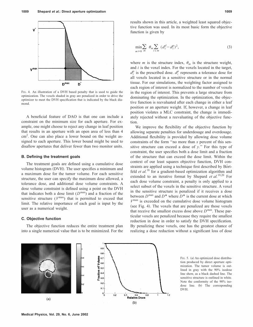
FIG. 4. An illustration of a DVH based penalty that is used to guide the

optimization. The voxels shaded in gray are penalized in order to drive the

optimizer to meet the DVH specification that is indicated by the black dia-

mond.

FIG. 5. ~a! An optimized dose distribu-

tion produced by direct aperture opti-

mization. The tumor volume is out-

lined in gray with the 90% isodose

line show, as a black dashed line. The

sensitive structure is outlined in white.

Note the conformity of the 90% iso-

dose line. ~b! The corresponding

DVH.



uniformity in the tumor. It should be noted that the subset of

penalized voxels changes with each iteration.

D. Monte Carlo dose calculation

We have used the EGS4/BEAM21 Monte Carlo system as

our dose calculation engine. The BEAM code was used to

simulate an Elekta SL20 linac equipped with a MLC. An-

other EGS4 user code, DOSXYZ, was employed to obtain

3-D dose distributions on phantoms and on CT images. The

BEAM code outputs the phase-space data, which include all

the particle information ~i.e., the charge, position, direction,

energy, and history tag for each particle!. These phase-space

data are then used as the input to the dose calculation. The

linac simulation was performed in two steps. First, the com-

ponents above the MLC ~including target, primary collima-

tor, flattening filters, ion chambers, and mirror! were simu-

lated. The remaining components ~MLC, diaphragms, and air

gap! were then simulated starting with the phase space files

scored in the first step on a plane immediately above MLC.

For our SL20 linac, the first simulation only needed to be

performed once. The later simulation was carried out for a

series of rectangular field shapes and for any field apertures

generated by the direct aperture optimization routine. The

entire Monte Carlo process has previously been validated.22

The pencil beam dose distributions are computed before

the optimization using the DOSXYZ code with a rectangular

MLC shape large enough to cover the BEV of the target plus

a margin. These pencil beams are generated at the predeter-

mined beam angles. The total dose from each aperture is

computed as a sum of all of the unblocked pencil beams.

Each field shape undergoes hundreds of modifications during

the optimization. After each change in leaf position, the af-

fected pencil beams are simply added or subtracted from the

total dose distribution. This dose calculation can thus be per-

formed very rapidly. At the end of the optimization, a final

FIG. 6. A plot of the best objective function vs iteration. Note that with

simulated annealing the current objective function both increases and de-

creases during the optimization.

FIG. 7. The three aperture shapes and

corresponding intensity map for one

beam direction. The open area of each

aperture is shown in black.



dose calculation is performed using the optimized apertures

and aperture weights.

Several computer programs were developed to automate

the entire Monte Carlo process. These programs include ~i!

the conversion of actual beam setup coordinate system ~e.g.,

isocenter coordinates, angles of gantry, collimator and

couch! of the linac to the coordinate system for the Monte

Carlo calculation, ~ii! the generation of Monte Carlo input

files for all pencil beams, and ~iii! the translation of leaf

positions produced by the DAO algorithm into a format suit-

able for the BEAM code. The Monte Carlo calculation of the

pencil beams was run in parallel on 12 Pentium III 750 MHz

PCs. The computation time required to generate pencil

beams ranges from 2 to 6 h depending on the number of

beams and their field sizes.

E. Number of intensity levels

With DAO, the intensity of each aperture is allowed to

vary continuously. In combination, these apertures produce

complex intensity maps. The relationship between the num-

ber of intensity levels per beam direction and the number of

apertures per beam direction can be expressed as

Nn52n21, ~4!

where n is the number of apertures and N is the possible

number of intensity levels. It is thus possible to have seven

intensity levels when just three apertures are used. With five

apertures, the number of possible intensity levels jumps to

31. Sixty-three intensity levels are possible when six aper-

tures are used. Consequently, highly modulated intensity pat-

terns can be produced using a small number of apertures per

beam direction. This offers a significant advantage over the

traditional two-step process where the number of apertures is

typically two to three times the number of intensity levels.7

For instance, for 15 intensity levels, DAO requires 4 aper-

tures as compared to the 30 to 45 apertures required by tra-

ditional algorithms.

F. Phantom studies

Initial tests of the DAO algorithm were performed on a

cylindrical phantom. Results are presented for a concave tar-

get with an adjacent sensitive structure. Seven equispaced

beam angles were used with three apertures shapes per angle.

Each pencil beam projected to 1.0 cm by 0.5 cm at isocenter.

The voxel size was 0.2 cm by 0.2 cm by 0.5 cm. The opti-

mization included 5691 voxels in the target, 1952 voxels in

the sensitive structure, and 7567 normal tissue voxels. A total

of 441 variables were included in the optimization ~10 leaf

pairs 3 2 leafs per pair 3 7 angles 3 3 apertures per angle

1 21 aperture weights!.

For a C-shaped target, optimizations were run using 1, 3,

5, 7, and 9 apertures per beam direction. This test was de-

signed to examine the extent to which the quality of the dose

distribution is related to the number of apertures per beam

direction. The pencil beam size was 1.0 cm by 0.5 cm pro-

jected to the isocenter, and a total of 12 702 voxels were

included in the optimization.

G. Prostate patient

Additional tests were performed on a prostate patient.

Seven equispaced beam angles were used with three aper-

tures per angle. A pencil beam size of 1 cm by 0.5 cm was

used with a total of 24 735 voxels included in the optimiza-

TABLE I. The objective function and corresponding optimization time for the

C-shaped target run with 1, 3, 5, 7, and 9 apertures per beam angle. Note

that as the number apertures per beam angle increases there is a correspond-

ing improvement in the objective function value.

No. of apertures

Objective

function

Optimization

time ~min!

1 56.82 0.92

3 22.04 3.42

5 15.66 6.02

7 14.30 12.20

9 11.48 18.15

FIG. 8. ~a! A predicted dose distribution for direct aperture optimization

using seven beam angles with three apertures for each. The inner line is the

95% isodose line while the outer line is the 50% isodose line. ~b! The

measured dose distribution as determined from a scanned film after delivery

to the cylindrical phantom. The 95% and 50% isodose lines are shown.

FIG. 9. An optimized dose distribution for a c-shaped target with a centrally

located sensitive structure. In this case seven beams angles were used with

seven apertures per beam direction. The target is outlined in white.



tion. The voxel size was 0.4 cm by 0.4 cm by 0.3 cm. The

sensitive structures in this case included the rectum and blad-

der.

H. Head and neck patient

Results are shown for a head and neck case. In this case

seven beam angles were used with three apertures per beam

angle. The sensitive structures included the eyes, the optic

nerves, the spinal cord, and the brain stem. Each pencil beam

projected to 1 cm by 0.5 cm at isocenter. A voxel size of 0.3

cm by 0.3 cm by 0.3 cm was used and a total of 22 255

voxels were scored during the optimization.

I. Consistency test

A key advantage of the use of a stochastic optimization

approach such as simulated annealing is the ability to avoid

local minima. In practice, however, the avoidance of local

minima is dependent upon the annealing schedule, the choice

of initial temperature, the number of iterations performed at

each temperature, and how much the temperature is decre-

mented at each step as the cooling proceeds. Consequently,

one must balance the need for a short optimization time with

the desire to avoid local minima. To address this issue, we

present results obtained for the head and neck patient using

100 different random number seeds. Our standard cooling

FIG. 10. Dose volume histogram plots for the c-shape target run using 1, 3,

5, 7, and 9 apertures per beam direction. ~a! DVH for the target. Note that

the target dose uniformity improves with each increase in the number of

apertures. ~b! DVH for the centrally located critical structure. Note that the

dose to the critical structure is reduced with each increase in the number of

apertures.

FIG. 11. Optimized treatment plan and corresponding DVH for a patient

with prostate cancer using seven equispaced beam angles and three aper-

tures per beam direction. The 95%, 60%, and 30% isodose lines are shown.



schedule was used and each optimization was terminated af-

ter 10 000 successful iterations. The extent to which local

minima are affecting the quality of the final solution should

be reflected in the degree of variation among these plans.

J. Comparison with a commercial inverse-planningsystem

The first phantom case and the head and neck patient were

each optimized using a commercial inverse-planning system

~CORVUS, Nomos Corporation, Sewickly, PA!. CORVUS

makes use of the traditional two-step approach to inverse

planning in which an optimized pencil beam intensity pattern

is translated into a set of deliverable apertures. This compari-

son is designed to illustrate the extent to which DAO can

match the quality of dose distribution produced by the con-

ventional two-step approach to IMRT. The comparison also

serves to illustrate the extent to which DAO can reduce the

number of segments and the required number of monitor

units to deliver a step-and-shoot plan.

III. RESULTS

A. Phantom results

In Fig. 5, the optimized dose distribution and the corre-

sponding DVH are shown for the cylindrical phantom with a

concave target and an adjacent sensitive structure. Seven

equispaced beam angles were used with three apertures per

angle. Note that the 90% isodose line conforms tightly to the

boundary of the tumor volume. This optimization was per-

formed in 3.35 min on a 1.2 GHz PC running LINUX.

Prior to the optimization, it was specified that the optimi-

zation would stop after 4000 successful iterations. An itera-

tion is considered successful if a change results in either a

decrease in the objective function value or an increase in the

objective function value that passes the probability con-

straint. In Fig. 6, the objective function value for this case is

plotted versus the iteration number. The change in objective

function is less than 1% after 2000 iterations. Figure 6 plots

both the current objective function value and the best objec-

tive function value. These two curves are not identical, be-

cause the simulated annealing algorithm will accept some

changes that increase the objective function’s value. At the

end of the optimization, the optimizer outputs those settings

that provided the best objective function value.

FIG. 12. An axial ~a! and sagittal ~b! image of the dose distribution for a

head and neck patient. Seven beam angles are used with three apertures per

beam angle. The tumor volume is outlined in white and the dark dose-cloud

shows the 95% isodose coverage. The 50% isodose line is plotted as a thick

gray line.

FIG. 13. An optimization was run 100 times with different random number

seeds. This plot shows the results of fitting the histogram of final objective

functions to a Gaussian. The error bars are stastical.



We should note that the required number of iterations var-

ies depending upon both the complexity and size the target

shape along with the number of variables included in the

optimization. Although we choose to use the number of suc-

cesses as our termination criteria, any of a number of other

means could be used to specify the termination point.

In Fig. 7, the aperture shapes for one beam direction are

shown along with the corresponding intensity map. Each

shape meets the constraints imposed by the Elekta MLC.

Note that in combination, the three apertures produce six

nonzero beam intensities from this beam angle.

The accuracy of delivery with DAO has been validated

using our cylindrical phantom. Figure 8 shows a comparison

between predicted and measured results. This plan was de-

livered in approximately 7 min on an Elekta SL20 linear

accelerator. In comparing the measured and predicted dose

distributions, the 95% isodose lines agreed within 3 mm.

For the C-shaped target shown in Fig. 9, the DAO algo-

rithm was run using 1, 3, 5, 7, and 9 apertures per beam

direction. This test was designed to examine the extent to

which the quality of a plan is related to the number of aper-

tures. The pronounced nature of the concavity in this case

makes it very difficult to simultaneously obtain a uniform

target dose and significant sparing of the sensitive structure.

Figure 9 shows the dose distribution obtained using seven

apertures.

The final objective function for each of these optimiza-

tions is provided in Table I. With each increase in the number

of apertures, the optimizer is provided with a corresponding

increase in flexibility. Consequently, the final objective func-

tion value decreased with each increase in the number of

apertures per beam direction. The results are compared in a

DVH format in Fig. 10. Table I also lists the optimization

time for each run. Note that the optimization time increases

as the number of apertures increase. This is related to the

increase in the number of variables that need to be opti-

mized.

FIG. 14. The resulting dose volume histograms for the best and worst results obtained from 100 separate optimizations. Note that only modest differences are

seen in the DVHs.



B. Prostate patient

In Fig. 11, results are shown from the application of DAO

to a patient with prostate cancer. A conformal dose distribu-

tion has been produced using seven equispaced beam angles

and three apertures per angle. This optimization was per-

formed in 5 min on a 1.2 GHz PC.

C. Head and neck results

In Fig. 12, isodose distributions are shown for a sagittal

and an axial slice for a head and neck case optimized using

DAO. Seven beam angles were used with three apertures per

beam angle. This case is particularly difficult due to the

proximity of the eyes, the optic nerves, and the brainstem.

D. Result of consistency test

For the head and neck case described above, 100 separate

optimizations were performed with a different random num-

ber seed used in each case. In all cases, three apertures per

beam direction were used along with the same prescription

parameters. Each optimization was terminated after 10 000

successful iterations, and the optimization times varied be-

tween 6 and 7 min. The resulting histogram of final objective

function values was fit to a Gaussian distribution. The results

are plotted in Fig. 13. The resulting fit parameters are a mean

of 5.2 and a standard deviation of 0.07. The minimum objec-

tive function value from the 100 runs was 4.95 and the maxi-

mum value was 5.41. For these two extremes, the resulting

dose volume histograms are plotted in Fig. 14. Note that only

modest differences in the DVHs are seen. If a slower cooling

schedule was used in combination with a longer optimization

time, these differences could be further minimized. We are,

however, satisfied that the schedule that we are using strikes

an appropriate balance between the need for a short optimi-

zation and the need to avoid local minima.

E. Comparison with CORVUS

For the first phantom case, a treatment plan was op-

timized using CORVUS with the identical beam arrange-

ment as that applied using the DAO approach. The optimized

dose distribution and corresponding DVH are plotted in

Fig. 15. A DVH comparison between DAO and CORVUS

~see Fig. 16! demonstrates that similar dosimetric results

were obtained. In the phantom case, the DAO plan in-

cluded a total of 21 apertures as compared with 144 apertures

in the CORVUS plan, an 85% reduction in the number

of apertures. The DAO plan required 500 monitor units

to deliver the prescribed dose of 200 cGy. This is a 74%

reduction as compared to the CORVUS plan, which used

1860 monitor units in order to deliver the same dose. If

both plans could be delivered with 400 MU/min machine

dose rate, the beam on time for delivering the CORVUS

plan and the DAO plan would be 4.25 min and 1.25 min,

respectively. However, a more dramatic difference is seen

on linear accelerators that require an intersegment delay

time. For a seven second intersegment delay, the total delay

time between segments would amount to 16.8 min for the

CORVUS plan as compared with 2.45 min with the DAO

plan. Table II outlines the comparison between the two sys-

tems.

In Fig. 17 a DVH comparison is provided between DAO

and CORVUS for the head and neck patient. This patient had

previously been treated in our clinic using the CORVUS

plan. The same seven beam angles were used in each case.

In comparing the dose volume histograms, it can be seen

FIG. 15. Results produced by CORVUS for the same setup shown in Fig. 5. ~a! The optimized dose distribution for seven beam angles with three intensity

levels per beam direction. ~b! The corresponding DVH.



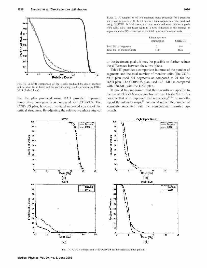
that the plan produced using DAO provided improved

tumor dose homogeneity as compared with CORVUS. The

CORVUS plan, however, provided improved sparing of the

critical structures. By adjusting the relative weights assigned

to the treatment goals, it may be possible to further reduce

the differences between these two plans.

Table III provides a comparison in terms of the number of

segments and the total number of monitor units. The COR-

VUS plan used 221 segments as compared to 21 for the

DAO plan. The CORVUS plan used 1761 MU as compared

with 338 MU with the DAO plan.

It should be emphasized that these results are specific to

the use of CORVUS in conjunction with an Elekta MLC. It is

possible that with improved leaf sequencing23,24 or smooth-

ing of the intensity maps,25 one could reduce the number of

segments associated with the conventional two-step ap-

proach.

TABLE II. A comparison of two treatment plans produced for a phantom

study, one produced with direct aperture optimization, and one produced

using CORVUS. In both cases, the same setup and same treatment goals

were used. Note that DAO leads to a 85% reduction in the number of

segments and a 74% reduction in the total number of monitor units.

Direct aperture

optimization CORVUS

Total No. of segments 21 144

Total No. of monitor units 500 1860

FIG. 16. A DVH comparison of the results produced by direct aperture

optimization ~solid lines! and the corresponding results produced by COR-

VUS ~dashed lines!.

FIG. 17. A DVH comparison with CORVUS for the head and neck patient.



Comparing CORVUS with DAO, the impact of leakage

and the tongue and groove effect would be more pronounced

with CORVUS due to the large number of beam segments. In

addition, the influence of patient motion would be increased

due to the use of beam segments that are small in size.1 Both

of these considerations decrease the accuracy of the dose

delivery.

IV. DISCUSSION

As compared with conventional IMRT planning tech-

niques, DAO is able to produce comparable dose conformity

with more efficient treatment deliveries. The reduction in the

number of beam segments not only improves delivery effi-

ciency, it also makes it easier to perform the required quality

assurance ~QA! procedures. Concerns regarding the dosim-

etric effects associated with current IMRT delivery, such as

the use of small MUs, tongue and grove effects, and head

scatter uncertainties for very small off-axis fields, are greatly

reduced.

Another benefit of this technique is that the user is given

considerable control over the complexity of the treatment

plan. For instance, if the user prescribes one aperture per

beam direction, a 3D conformal plan is produced; if the user

prescribes five or six apertures per beam direction, a highly

modulated IMRT plan can be produced. With this technique,

one can take an incremental approach to the implementation

of IMRT by starting with two apertures per beam direction

and gradually increasing to five or six.

Another important feature of this tool is the flexibility of

simulated annealing algorithm. One can easily replace the

least squares objective function, which is based on the physi-

cal dose distribution with a biological objective function

such as the equivalent uniform dose, TCP, or P1.26–32 Due to

their highly nonlinear nature, biological objective can be dif-

ficult to implement into other mathematical programming

formulations in a robust fashion.

DAO can also be applied to the optimization of intensity

modulated arc therapy ~IMAT!.33 With IMAT optimization,

one can specify the maximum number of arcs as input to the

optimizer. Additional constraints need to be added to ensure

that changes in the aperture shape from one beam angle to

the next do not violate constraints on the maximum leaf ve-

locity. Our IMAT results will be presented in a future publi-

cation. We will also present results showing how this tech-

nique can be used to produce hybrid plans that combine

rotational and fixed field IMRT.34

V. CONCLUSIONS

We have developed an IMRT inverse planning strategy

using direct aperture optimization. The MLC constraints are

incorporated into the optimization algorithm, therefore elimi-

nating the need for leaf sequencing. Results show that highly

conformal IMRT treatment plans can typically be produced

using five or fewer apertures per beam direction. This tool

improves both the efficiency and the accuracy of IMRT de-

livery.

ACKNOWLEDGMENTS

This research was partially supported by National Science

Foundation Grant No. ACI-0113051 and by National Insti-

tute of Health Grant No. R29CH66075. The authors would

like to thank Timothy Holmes for his contribution to this

work. Finally, the authors thank Mark Symons, Peter Maton,

and Rajesh Raut of Elekta for their assistance.

1T. Bortfeld, D. H. Haler, T. J. Waldron, and A. L. Boyer, ‘‘X-ray com-

pensation with multileaf collimators,’’ Int. J. Radiat. Oncol., Biol., Phys.

28, 723–739 ~1994!.2C. S. Chui, T. LoSasso, and S. Spirou, ‘‘Dose calculation for photon

beam with intensity modulation generated by dynamic jaw or multileaf

collimation,’’ Med. Phys. 21, 1237–1244 ~1994!.3 J. M. Galvin, X. G. Chen, and R. M. Smith, ‘‘Combining multileaf field

to modulate fluence distributions,’’ Int. J. Radiat. Oncol., Biol., Phys. 27,

697–705 ~1993!.4S. Webb, ‘‘Optimizing the planning of intensity-modulated radiotherapy,’’

Phys. Med. Biol. 39~12!, 2229–2246 ~1994!.5S. Webb, ‘‘Configuration options for intensity-modulated radiation

therapy using multiple static fields shaped by a multileaf collimator,’’

Phys. Med. Biol. 43~2!, 241–260 ~1998!.6S. Webb, ‘‘Configuration options for intensity-modulated radiation

therapy using multiple static fields shaped by a multileaf collimator. II:

Constraints and limitations on 2D modulation,’’ Phys. Med. Biol. 43~6!,

1481–1495 ~1998!.7P. Xia and L. J. Verhey, ‘‘Mutileaf collimation leaf sequencing algorithm

for intensity modulated beams with multiple static segments,’’ Med.

Phys. 25, 1424–1434 ~1998!.8 J. Tervo and P. Kolmonen, ‘‘A model for the control of a multileaf colli-

mator in radiation therapy treatment planning,’’ Inverse Probl. 16, 1875–

1895 ~2000!.9W. DeGersem, F. Claus, C. DeWagter, B. VanDuyse, and W. DeNeve,

‘‘Leaf position optimization for step-and-shoot IMRT,’’ Int. J. Radiat.

Oncol., Biol., Phys. 51~5!, 1371–1388 ~2001!.10R. Rardin, Optimization in Operations Research ~Prentice Hall, Engle-

wood Cliffs, NJ, 1998!.11S. Kirkpatrick, C. D. Gelatt, Jr., and M. P. Vecchi, ‘‘Optimization by

simulated annealing,’’ Science 220~4598!, 671–680 ~1993!.12S. Geman and D. Geman, ‘‘Stochastic relaxation, Gibbs distribution and

the Bayesian restoration in images,’’ IEEE Trans. Pattern Anal. Mach.

Intell. 6~6!, 731–741 ~1984!.13M. Pincus, ‘‘A Monte Carlo Method for the approximate calculation of

certain types of constrained optimization problems,’’ Oper. Res. 18,

1225–1228 ~1970!.14V. Cerny, ‘‘A thermodynamic approach to the traveling salesman prob-

lem: An efficient simulation algorithm,’’ Report, Comenius University,

Brathislava, Czechoslovakia, 1982.15K. Binder and D. Stauffer, ‘‘A simple introduction to Monte Carlo simu-

lations and some specialized topics,’’ in Statistical Physics, edited by K.

Binder ~Springer-Verlag, Berlin, 1985!, pp. 1–36.16T. J. Jordan and P. C. Williams, ‘‘The design and performance character-

istics of a multileaf collimator,’’ Phys. Med. Biol. 39, 231–251 ~1994!.17Multileaf Collimator (MLC) Operator’s Manual for MLC SA1, Philips

Medical Systems, Document No. 4522 984 40891/764, Appendix C,

1993.

TABLE III. A comparison of two treatment plans for a head and neck patient,

one produced with direct aperture optimization, and one produced using

CORVUS. In both cases, the same setup beam arrangement and treatment

goals were used.

Direct apertureoptimization CORVUS

Total No. of segments 21 221

Total No. of monitor units 338 1761



18T. Bortfeld, J. Stein, and K. Preiser, ‘‘Clinically Relevant Intensity Modu-

lation Optimization Using Physical Criteria,’’ in Proceeding of the XII

International Conference on the Use of Computers in Radiation Therapy,

Salt Lake City, UT ~1997!.19D. M. Shepard, G. H. Olivera, P. J. Reckwerdt, and T. R. Mackie, ‘‘It-

erative approaches to dose optimization’’, Phys. Med. Biol. 45, 69–90

~1999!.20Chapter 15: ‘‘Tomotherapy,’’ The Modern Technology of Radiation On-

cology, a Compendium for Medical Physicists and Radiation Oncolo-

gists, edited by J. Van Dyck, G. H. Olivera, D. M. Shepard, K. Ruchala,

J. S. Aldridge, J. Kapatoes, E. E. Fitchard, P. J. Reckwerdt, G. Fang, J.

Balog, J. Zachman, and T. R. Mackie ~Medical Physics, Madison, WI,

1999!.21D. W. O. Rogers, B. A. Faddegon, G. X. Ding, C. M. Ma, J. Wei, and T.

R. Mackie, ‘‘BEAM: a Monte Carlo code to simulate radiotherapy treat-

ment unit,’’ Med. Phys. 22, 503–524 ~1995!.22X. A. Li, L. Ma, S. Naqvi, R. Shih, and C. Yu, ‘‘Monte Carlo dose

verification for intensity modulated arc therapy,’’ Phys. Med. Biol. 46~9!,

2269–2282 ~2001!.23M. Langer, V. Thai, and L. Papiez, ‘‘Improved leaf sequencing reduces

segments or monitor units needed to deliver IMRT using multileaf colli-

mators,’’ Med. Phys. 28, 2450–2458 ~2001!.24 J. Dai and Y. Zhu, ‘‘Minimizing the number of segments in a delivery

sequence for intensity-modulated radiation therapy with a multileaf col-

limator,’’ Med. Phys. 28, 2113–2120 ~2001!.25S. V. Spirou, N. Fournier-Bidoz, J. Yang, C. S. Chui, and C. C. Ling,

‘‘Smoothing intensity-modulated beam profiles to improve the efficiency

of delivery,’’ Med. Phys. 28, 2105–2112 ~2001!.26P. Stavrev, N. Stavreva, A. Niemierko, and M. Goitein, ‘‘Generalization

of a model of tissue response to radiation based on the idea of functional

subunits and binomial statistics,’’ Phys. Med. Biol. 46, 1501–1518

~2001!.27L. C. Jones and P. W. Hoban, ‘‘Treatment plan comparison using equiva-

lent uniform biologically effective dose ~EUBED!,’’ Phys. Med. Biol.

45~1!, 159–170 ~2000!.28A. Niemierko, ‘‘Radiobiological models of tissue response to radiation in

treatment planning systems,’’ Tumori 84~2!, 140–143 ~1998!.29A. Niemierko, ‘‘Reporting and analyzing dose distributions: a concept of

equivalent uniform dose,’’ Med. Phys. 24, 103–110 ~1997!.30A. Brahme, ‘‘Individualizing cancer treatment: biological optimization

models in treatment planning and delivery’’ Int. J. Radiat. Oncol., Biol.,

Phys. 49~2!, 327–337 ~2001!.31A. Brahme, ‘‘Biologically based treatment planning,’’ Acta Oncol.

38~Suppl. 13!, 61–68 ~1999!.32A. Brahme, ‘‘Optimized radiation therapy based on radiobiological ob-

jectives,’’ Semin. Radiat. Oncol. 9~1!, 35–47 ~1999!.33M. A. Earl, D. M. Shepard, X. A. Li, and C. X. Yu, ‘‘Inverse planning for

intensity modulated arc therapy using direct aperture optimization,’’ Int.

J. Radiat. Oncol., Biol., Phys. 51~3!, Suppl. 1, 404 ~2001!.34C. X. Yu and J. Li, ‘‘Angular Cost—A new concept for broad-scope

planning optimization,’’ Int. J. Radiat. Oncol., Biol., Phys. 51~3!,

Suppl. 1, 406 ~2001!.



Direct aperture optimization: A turnkey solution for step-and-shoot

Documents

Transcript of Direct aperture optimization: A turnkey solution for step-and-shoot