Direct and large-eddy simulation of inert and reacting ...
251
Technische Universit¨ at M ¨ unchen Fachgebiet Str¨ omungsmechanik Direct and large-eddy simulation of inert and reacting compressible turbulent shear layers Inga Mahle Vollst¨ andiger Abdruck der von der Fakult¨ at f¨ ur Maschinenwesen der Technischen Universit¨ at M¨ unchen zur Erlangung des akademischen Grades eines Doktor-Ingenieurs genehmigten Dissertation. Vorsitzender: Univ.-Prof. Dr.-Ing. habil. N. A. Adams Pr¨ ufer der Dissertation: 1. Univ.-Prof. Dr.-Ing., Dr.-Ing. habil. R. Friedrich i.R. 2. Univ.-Prof. W. H. Polifke Ph.D. (CCNY) Die Dissertation wurde am 16.4.2007 bei der Technischen Universit¨ at M¨ unchen eingereicht und durch die Fakult¨ at f¨ ur Maschinenwesen am 10.7.2007 angenommen.
Transcript of Direct and large-eddy simulation of inert and reacting ...

Technische Universitat MunchenFachgebiet Stromungsmechanik
Direct and large-eddy simulationof inert and reacting
compressible turbulent shear layers
Inga Mahle
Vollstandiger Abdruck der von der Fakultat fur Maschinenwesen der Technischen UniversitatMunchen zur Erlangung des akademischen Grades eines
Doktor-Ingenieurs
genehmigten Dissertation.
Vorsitzender: Univ.-Prof. Dr.-Ing. habil. N. A. AdamsPrufer der Dissertation:
1. Univ.-Prof. Dr.-Ing., Dr.-Ing. habil. R. Friedrich i.R.2. Univ.-Prof. W. H. Polifke Ph.D. (CCNY)
Die Dissertation wurde am 16.4.2007 bei der Technischen Universitat Munchen eingereicht unddurch die Fakultat fur Maschinenwesen am 10.7.2007 angenommen.


Abstract
In the first part of the thesis, Direct Numerical Simulations (DNS) of temporally evolving, tur-bulent, compressible shear layers are discussed. Simulations at three different convective Machnumbers (0.15, 0.7 and 1.1) were performed for both, inert and infinitely fast reacting gases. Allsimulations were continued beyond the onset of a self-similar state in order to guarantee statisticsof general value. Self-similarity manifested itself by a collapse of suitably normalized profiles offlow variables and a constant momentum thickness growth rate. During this state, the Reynoldsnumber based on the vorticity thickness of the shear layers was between 10000 and 40000 andtherefore in a fully turbulent regime. The relevance of the achieved results and parameter rangesfor practical applications can be seen from the fact that shear (or mixing) layers develop wheninjecting fuel into the combustion chamber of an engine. Here, a good mixing of fuel and oxidizeris of great interest for an efficient combustion process.
The focus of the DNS data analyses was on the effects of compressibility and heat release due tocombustion on turbulence and scalar mixing. Both phenomena, compressibility and heat release,were studied separately as well as in combination. Increasing compressibility, i.e. increasingconvective Mach number, resulted in a stabilization of the mixing layers: Instantaneous fields offlow quantities became smoother, there were less turbulent fluctuations and the growth rate of themixing layers reduced. The latter effect was related to a reduction in the production rate of thestreamwise Reynolds stress and a reduction in the pressure-strain correlations caused by changesin the fluctuating pressure field. When heat release was present, the effects of compressibilitywere similar as for the inert mixing layers, but they were less distinct, e.g. the reduction of thegrowth rate with increasing Mach number was comparatively smaller. At first sight, heat releasealone had similar consequences as compressibility: A stabilization of the shear layers, flow fieldswith lower levels of fluctuations and smaller spreading rates. However, when studied in moredetail, it could be seen that the consequences of heat release, were mainly ’mean density effects’,i.e. a result of the reduction of the mean density by the high temperatures in the vicinity of theflame sheets. This was not the case for the compressibility effects. Therefore, it is important todistinguish between compressibility and heat release effects, even though they share the propertyto be both detrimental for the turbulent mixing process.
In the second part of the thesis, Large Eddy Simulations (LES) of shear layers at a convectiveMach number of 0.15 were performed. By a coarsening of the grid, large reductions of computa-tional time were achieved. A deconvolution approach in the form of a single explicit filtering stepwas validated successfully for inert and reacting mixing layers by comparison with DNS data.For the LES with chemical reactions, two differently detailed chemistry models were used for thefiltered chemical source term: one model taking into account the same infinitely fast, irreversible,global reaction as in the DNS and one flamelet model. The particular formulation of the flameletequations allowed not only to take into account multistep Arrhenius chemistry, but also detaileddiffusion mechanisms. The evaluation of the results obtained with two different descriptions ofthese mechanisms - one with Soret and Dufour effects as well as multicomponent diffusion and

one without - showed differences for both, laminar flamelets and turbulent mixing layers, inquantities related to the flame dynamics and in the extinction behaviour.

Acknowledgements
First of all, I would like to thank my supervisor Prof. Dr.-Ing. habil. Rainer Friedrich for theopportunity to perform this work at the ’Fachgebiet Stromungsmechanik’. He gave me constantguidance and support and was always ready to answer questions or to discuss various aspects.
I am also thankful to Prof. Dr. Joseph Mathew for giving me the opportunity to spend four monthsin his lab at the Indian Institute of Science in Bangalore. I appreciate his gracious hospitality andthe fruitful discussions that we had. The final outcome of our joint work has been very rewarding.
I would also like to thank Prof. W. Polifke Ph.D. (CCNY) for taking over the role of the secondexaminer and Prof. Dr.-Ing. habil. N. Adams for leading the board of examiners.
My thanks go also to the High Performance Computing Group of the ’Leibniz Rechenzentrum’(LRZ) for providing help and support at nearly all times of the day, all days of the week. Thecomputations of this work were performed on the Hitachi-SR8000 and the Altix 4700 of the LRZ.Financial contributions came from the Federal Ministry of Education and Research (BMBF) un-der grant number 03FRA1AC and from ’Bayerischer Forschungsverbund fur Turbulente Verbren-nung’ (FORTVER).
Without my colleagues and the mutual support and encouragement within our group, this workwould not have been imaginable. In this context, I would like to mention especially Dr.-Ing.Holger Foysi who gave me a lot of help and advice concerning the numerical codes and evaluationprograms. I would also like to thank Prof. Alexandre Ern from CERMICS, ENPC (France) forproviding the code EGlib.
Last but not least, I am deeply grateful to my family, in particular to my parents and grandparents,for supporting me throughout the process of this work and throughout all my life.
Garching, March 2007Inga Mahle

Contents
1 Introduction 1
2 DNS of inert compressible turbulent shear layers 4
2.1 Introduction and literature survey . . . . . . . . . . . . . . . . . . . . . . . . . . . . . . . 4
2.2 The DNS code for inert gas mixtures . . . . . . . . . . . . . . . . . . . . . . . . . . . . . 6
2.2.1 Navier-Stokes equations for a gas mixture . . . . . . . . . . . . . . . . . . . . . . 6
2.2.2 The numerical method . . . . . . . . . . . . . . . . . . . . . . . . . . . . . . . . 8
2.3 Test cases . . . . . . . . . . . . . . . . . . . . . . . . . . . . . . . . . . . . . . . . . . . 8
2.4 Results and analysis . . . . . . . . . . . . . . . . . . . . . . . . . . . . . . . . . . . . . . 10
2.4.1 The structure of the compressible shear layers . . . . . . . . . . . . . . . . . . . . 10
2.4.1.1 Inert shear layer at Mc = 0.15 . . . . . . . . . . . . . . . . . . . . . . 11
2.4.1.2 Inert shear layer at Mc = 0.7 . . . . . . . . . . . . . . . . . . . . . . . 12
2.4.1.3 Inert shear layer at Mc = 1.1 . . . . . . . . . . . . . . . . . . . . . . . 14
2.4.2 The self-similar state . . . . . . . . . . . . . . . . . . . . . . . . . . . . . . . . . 17
2.4.3 Check of resolution, domain sizes and filtering . . . . . . . . . . . . . . . . . . . 23
2.4.4 The effect of compressibility . . . . . . . . . . . . . . . . . . . . . . . . . . . . . 25
2.4.4.1 Turbulence characteristics . . . . . . . . . . . . . . . . . . . . . . . . . 25
Mean flow variables . . . . . . . . . . . . . . . . . . . . . . . . . . . . . 25
Reynolds stresses, turbulent kinetic energy and anisotropies . . . . . . . . 26
Reynolds stress transport equations . . . . . . . . . . . . . . . . . . . . . 28
Analysis of the reduced growth rate . . . . . . . . . . . . . . . . . . . . . 32
Pressure-strain terms . . . . . . . . . . . . . . . . . . . . . . . . . . . . . 34
TKE transport equation . . . . . . . . . . . . . . . . . . . . . . . . . . . . 35
Thermodynamic fluctuations . . . . . . . . . . . . . . . . . . . . . . . . . 38
Correlations of thermodynamic fluctuations . . . . . . . . . . . . . . . . . 40
Behaviour of the pressure-strain correlations . . . . . . . . . . . . . . . . 41
Turbulent and gradient Mach numbers . . . . . . . . . . . . . . . . . . . . 46
Spectra . . . . . . . . . . . . . . . . . . . . . . . . . . . . . . . . . . . . 48

II CONTENTS
2.4.4.2 Scalar mixing . . . . . . . . . . . . . . . . . . . . . . . . . . . . . . . 49
Mean profile and variance . . . . . . . . . . . . . . . . . . . . . . . . . . 49
Scalar pdfs . . . . . . . . . . . . . . . . . . . . . . . . . . . . . . . . . . 50
Mixing efficiency . . . . . . . . . . . . . . . . . . . . . . . . . . . . . . . 52
Scalar variance transport equation . . . . . . . . . . . . . . . . . . . . . . 53
Scalar fluxes . . . . . . . . . . . . . . . . . . . . . . . . . . . . . . . . . 54
Transport equations of scalar fluxes . . . . . . . . . . . . . . . . . . . . . 55
Behaviour of the pressure-scrambling terms . . . . . . . . . . . . . . . . . 58
Spectra . . . . . . . . . . . . . . . . . . . . . . . . . . . . . . . . . . . . 60
2.4.4.3 Entrainment . . . . . . . . . . . . . . . . . . . . . . . . . . . . . . . . 61
Measurement of volumes . . . . . . . . . . . . . . . . . . . . . . . . . . . 61
Visual thickness . . . . . . . . . . . . . . . . . . . . . . . . . . . . . . . 63
Measurement of densities . . . . . . . . . . . . . . . . . . . . . . . . . . 63
Particle statistics . . . . . . . . . . . . . . . . . . . . . . . . . . . . . . . 65
Fractal nature of the mixing layer interface . . . . . . . . . . . . . . . . . 68
2.4.4.4 Shocklets . . . . . . . . . . . . . . . . . . . . . . . . . . . . . . . . . . 70
2.5 Summary and conclusions . . . . . . . . . . . . . . . . . . . . . . . . . . . . . . . . . . 76
3 DNS of infinitely fast reacting compressible turbulent shear layers 78
3.1 Introduction and literature survey . . . . . . . . . . . . . . . . . . . . . . . . . . . . . . . 78
3.2 The DNS code with an infinitely fast chemical reaction . . . . . . . . . . . . . . . . . . . 81
3.2.1 Infinitely fast chemistry . . . . . . . . . . . . . . . . . . . . . . . . . . . . . . . 81
3.2.2 Transport equations for infinitely fast reacting flows . . . . . . . . . . . . . . . . 83
3.2.3 The numerical method . . . . . . . . . . . . . . . . . . . . . . . . . . . . . . . . 84
3.3 Test cases . . . . . . . . . . . . . . . . . . . . . . . . . . . . . . . . . . . . . . . . . . . 84
3.4 Results and analysis . . . . . . . . . . . . . . . . . . . . . . . . . . . . . . . . . . . . . . 86
3.4.1 The structure of the infinitely fast reacting shear layers . . . . . . . . . . . . . . . 86
3.4.1.1 Infinitely fast reacting shear layer at Mc = 0.15 . . . . . . . . . . . . . 86
3.4.1.2 Infinitely fast reacting shear layers at Mc = 0.7 and Mc = 1.1 . . . . . 87
3.4.2 The self-similar state . . . . . . . . . . . . . . . . . . . . . . . . . . . . . . . . . 87
3.4.3 Check of resolution and domain sizes . . . . . . . . . . . . . . . . . . . . . . . . 89
3.4.4 Effects of compressibility and heat release . . . . . . . . . . . . . . . . . . . . . . 91
3.4.4.1 Mean heat release term . . . . . . . . . . . . . . . . . . . . . . . . . . 91
CONTENTS III
3.4.4.2 Turbulence characteristics . . . . . . . . . . . . . . . . . . . . . . . . . 91
Mean flow variables . . . . . . . . . . . . . . . . . . . . . . . . . . . . . 91
Reynolds stresses, turbulent kinetic energy and anisotropies . . . . . . . . 93
Reynolds stress transport equations . . . . . . . . . . . . . . . . . . . . . 96
Analysis of the reduced growth rate . . . . . . . . . . . . . . . . . . . . . 100
Pressure-strain terms . . . . . . . . . . . . . . . . . . . . . . . . . . . . . 101
TKE transport equation . . . . . . . . . . . . . . . . . . . . . . . . . . . . 102
Thermodynamic fluctuations . . . . . . . . . . . . . . . . . . . . . . . . . 105
Correlations of thermodynamic fluctuations . . . . . . . . . . . . . . . . . 106
Behaviour of the pressure-strain correlations . . . . . . . . . . . . . . . . 107
Turbulent and gradient Mach numbers . . . . . . . . . . . . . . . . . . . . 112
Spectra . . . . . . . . . . . . . . . . . . . . . . . . . . . . . . . . . . . . 113
3.4.4.3 Scalar mixing . . . . . . . . . . . . . . . . . . . . . . . . . . . . . . . 114
Mean profile and variance . . . . . . . . . . . . . . . . . . . . . . . . . . 115
Scalar pdfs . . . . . . . . . . . . . . . . . . . . . . . . . . . . . . . . . . 117
Mixing efficiency . . . . . . . . . . . . . . . . . . . . . . . . . . . . . . . 118
Scalar variance transport equation . . . . . . . . . . . . . . . . . . . . . . 119
Scalar fluxes . . . . . . . . . . . . . . . . . . . . . . . . . . . . . . . . . 120
Transport equations of scalar fluxes . . . . . . . . . . . . . . . . . . . . . 121
Spectra . . . . . . . . . . . . . . . . . . . . . . . . . . . . . . . . . . . . 123
3.4.4.4 Entrainment . . . . . . . . . . . . . . . . . . . . . . . . . . . . . . . . 124
Measurement of volumes . . . . . . . . . . . . . . . . . . . . . . . . . . . 124
Visual thickness . . . . . . . . . . . . . . . . . . . . . . . . . . . . . . . 126
Measurement of densities . . . . . . . . . . . . . . . . . . . . . . . . . . 127
Particle statistics . . . . . . . . . . . . . . . . . . . . . . . . . . . . . . . 128
Fractal nature of the mixing layer interface . . . . . . . . . . . . . . . . . 129
3.4.5 Shocklets . . . . . . . . . . . . . . . . . . . . . . . . . . . . . . . . . . . . . . . 131
3.5 Summary and conclusions . . . . . . . . . . . . . . . . . . . . . . . . . . . . . . . . . . 131

IV CONTENTS
4 LES of inert and infinitely fast reacting mixing layers 134
4.1 Introduction and literature survey . . . . . . . . . . . . . . . . . . . . . . . . . . . . . . . 134
4.2 Description of the LES method . . . . . . . . . . . . . . . . . . . . . . . . . . . . . . . . 139
4.2.1 Implicit Modeling Approach . . . . . . . . . . . . . . . . . . . . . . . . . . . . . 139
4.2.2 Applied filters . . . . . . . . . . . . . . . . . . . . . . . . . . . . . . . . . . . . 140
4.2.3 Filtered equations . . . . . . . . . . . . . . . . . . . . . . . . . . . . . . . . . . . 142
4.2.4 Modeling of the filtered heat release term . . . . . . . . . . . . . . . . . . . . . . 142
4.2.4.1 The filtered density function . . . . . . . . . . . . . . . . . . . . . . . . 144
4.2.4.2 The conditionally filtered scalar dissipation rate . . . . . . . . . . . . . 145
4.2.4.3 The filtered scalar dissipation rate . . . . . . . . . . . . . . . . . . . . . 146
4.3 Test cases . . . . . . . . . . . . . . . . . . . . . . . . . . . . . . . . . . . . . . . . . . . 146
4.4 Results and analysis . . . . . . . . . . . . . . . . . . . . . . . . . . . . . . . . . . . . . . 147
4.4.1 Inert mixing layers . . . . . . . . . . . . . . . . . . . . . . . . . . . . . . . . . . 147
4.4.1.1 Instantaneous fields . . . . . . . . . . . . . . . . . . . . . . . . . . . . 147
4.4.1.2 Profiles of averaged flow variables . . . . . . . . . . . . . . . . . . . . 148
4.4.1.3 Spectra . . . . . . . . . . . . . . . . . . . . . . . . . . . . . . . . . . . 151
4.4.1.4 Effect of filtering on dissipation rates . . . . . . . . . . . . . . . . . . . 153
4.4.1.5 Refinement of the grid . . . . . . . . . . . . . . . . . . . . . . . . . . . 154
4.4.2 Infinitely fast reacting mixing layers . . . . . . . . . . . . . . . . . . . . . . . . . 155
4.4.2.1 Instantaneous fields . . . . . . . . . . . . . . . . . . . . . . . . . . . . 155
4.4.2.2 Profiles of averaged flow variables . . . . . . . . . . . . . . . . . . . . 156
4.4.2.3 The filtered heat release term . . . . . . . . . . . . . . . . . . . . . . . 158
4.4.2.4 Spectra . . . . . . . . . . . . . . . . . . . . . . . . . . . . . . . . . . . 162
4.4.2.5 Effect of filtering on dissipation rates . . . . . . . . . . . . . . . . . . . 163
4.4.2.6 Refinement of the grid . . . . . . . . . . . . . . . . . . . . . . . . . . . 163
4.5 Summary and conclusions . . . . . . . . . . . . . . . . . . . . . . . . . . . . . . . . . . 164

CONTENTS V
5 LES of shear layers with chemical kinetic and detailed diffusion effects 167
5.1 Introduction and literature survey . . . . . . . . . . . . . . . . . . . . . . . . . . . . . . . 167
5.2 LES approach . . . . . . . . . . . . . . . . . . . . . . . . . . . . . . . . . . . . . . . . . 168
5.2.1 LES equations and models . . . . . . . . . . . . . . . . . . . . . . . . . . . . . . 168
5.2.2 Filtered heat release term and filtered species mass fractions . . . . . . . . . . . . 169
5.3 The flamelet database . . . . . . . . . . . . . . . . . . . . . . . . . . . . . . . . . . . . . 170
5.3.1 Detailed reaction scheme and Arrhenius chemistry . . . . . . . . . . . . . . . . . 170
5.3.2 Computation of detailed diffusion fluxes and of heat flux by EGlib . . . . . . . . . 172
5.3.3 The mixture fraction and its diffusivity . . . . . . . . . . . . . . . . . . . . . . . 173
5.3.4 Steady flamelet solutions . . . . . . . . . . . . . . . . . . . . . . . . . . . . . . . 174
5.4 Test cases . . . . . . . . . . . . . . . . . . . . . . . . . . . . . . . . . . . . . . . . . . . 175
5.5 Results and analysis . . . . . . . . . . . . . . . . . . . . . . . . . . . . . . . . . . . . . . 176
5.5.1 Flamelets with detailed and simplified diffusion . . . . . . . . . . . . . . . . . . . 176
5.5.2 Evaluation of the LES results . . . . . . . . . . . . . . . . . . . . . . . . . . . . 178
5.6 Summary and conclusions . . . . . . . . . . . . . . . . . . . . . . . . . . . . . . . . . . 185
6 Conclusions and outlook 186
A Appendix: The characteristic form of the Navier-Stokes equations 190
A.1 The one-dimensional equations . . . . . . . . . . . . . . . . . . . . . . . . . . . . . . . . 190
A.2 The three-dimensional equations in Cartesian coordinates . . . . . . . . . . . . . . . . . . 192
A.3 The source terms in the transport equations . . . . . . . . . . . . . . . . . . . . . . . . . 193
A.4 Specification of the transport equations for an ideal gas mixture . . . . . . . . . . . . . . . 195
A.5 Non-reflecting boundary conditions . . . . . . . . . . . . . . . . . . . . . . . . . . . . . 197

List of Tables
2.1 Geometrical parameters of the simulations inert-0.15, inert-0.7, inert-1.1. Thecomputational domain has the dimensions L1, L2 and L3 with N1, N2 and N3
grid points, respectively. The reference vorticity thickness δω, 0 is chosen suchthat it results in Reω,0 = 640. . . . . . . . . . . . . . . . . . . . . . . . . . . . . 9
2.2 Dimensionless times and Reynolds numbers at the beginning (index: B) and end(index: E) of the self-similar state . . . . . . . . . . . . . . . . . . . . . . . . . 19
2.3 Integral length scales . . . . . . . . . . . . . . . . . . . . . . . . . . . . . . . . 25
2.4 Values used in the analysis linking momentum thickness growth rate with pressure-strain rate Π11 for the inert test cases . . . . . . . . . . . . . . . . . . . . . . . . 32
2.5 Actual and approximated momentum thickness growth rates and relative errorsfor the inert test cases . . . . . . . . . . . . . . . . . . . . . . . . . . . . . . . . 33
2.6 Particle parameters: NP particles are initialized at τω,PB. They are situated ini-tially between x3 = x3,P1 and x3,P2 and between x3 = x3,P3 and x3,P4 . . . . . . 66
2.7 Statistics of displacements and elapsed times for growth of vorticity and mixturefraction along particle pathlines . . . . . . . . . . . . . . . . . . . . . . . . . . . 67
2.8 Fractal dimensions D of isosurfaces determined from the slopes of the curves inFigs. 2.175 to 2.176 and corresponding ones for ω = 0.2〈ω〉max and Y = 0.9 . . 68
3.1 Geometrical parameters of the simulations inf-0.15, inf-0.7, inf-1.1. The com-putational domain has the dimensions L1, L2 and L3 with N1, N2 and N3 gridpoints, respectively. The reference vorticity thickness δω,0 is chosen such that itresults in Reω,0 = 640. . . . . . . . . . . . . . . . . . . . . . . . . . . . . . . . 85
3.2 Dimensionless times and Reynolds numbers at the beginning (index: B) and end(index: E) of the self-similar state . . . . . . . . . . . . . . . . . . . . . . . . . 88
3.3 Integral length scales . . . . . . . . . . . . . . . . . . . . . . . . . . . . . . . . 91
3.4 Values used in the analysis linking momentum thickness growth rate with pressure-strain rate Π11 for the infinitely fast reacting test cases . . . . . . . . . . . . . . . 100
3.5 Actual and approximated momentum thickness growth rates and relative errorsfor the infinitely fast reacting test cases . . . . . . . . . . . . . . . . . . . . . . . 100
3.6 Averaged values (respective inert and reacting cases taken into account) used inthe analysis for each convective Mach number . . . . . . . . . . . . . . . . . . . 101
3.7 Actual and approximated momentum thickness growth rates and relative errors . 101

LIST OF TABLES VII
3.8 Particle parameters: NP particles are initialized at τω,PB. They are situated ini-tially between x3 = x3,P1 and x3,P2 and between x3 = x3,P3 and x3,P4 . . . . . . 128
3.9 Statistics of displacements and elapsed times for growth of vorticity and mixturefraction along particle pathlines . . . . . . . . . . . . . . . . . . . . . . . . . . . 129
3.10 Fractal dimensions D of isosurfaces . . . . . . . . . . . . . . . . . . . . . . . . 130
4.1 LES simulations . . . . . . . . . . . . . . . . . . . . . . . . . . . . . . . . . . . 147
5.1 Reaction scheme forH2/O2 combustion with pre-exponential factorsA, temperature-dependence coefficients β and activation energies E [113] . . . . . . . . . . . . 171

List of Figures
2.1 The configuration of temporally evolving shear layers . . . . . . . . . . . . . . 9
2.2 Case inert-0.15: Instantaneous mass fraction field of O2, x1-x3-plane in the mid-dle of the computational domain at τω = 83, isolines YO2 = 0.1 and 0.9 areshown . . . . . . . . . . . . . . . . . . . . . . . . . . . . . . . . . . . . . . . . 10
2.3 Case inert-0.15: Instantaneous mass fraction field of O2, x1-x3-plane in the mid-dle of the computational domain at τω = 286, isolines YO2 = 0.1 and 0.9 areshown . . . . . . . . . . . . . . . . . . . . . . . . . . . . . . . . . . . . . . . . 10
2.4 Case inert-0.15: Instantaneous mass fraction field of O2, x1-x3-plane in the mid-dle of the computational domain at τω = 409, isolines YO2 = 0.1 and 0.9 areshown . . . . . . . . . . . . . . . . . . . . . . . . . . . . . . . . . . . . . . . . 10
2.5 Case inert-0.15: Instantaneous mass fraction field of O2, x1-x3-plane in the mid-dle of the computational domain at τω = 533, isolines YO2 = 0.1 and 0.9 areshown . . . . . . . . . . . . . . . . . . . . . . . . . . . . . . . . . . . . . . . . 10
2.6 Case inert-0.15: Instantaneous mass fraction field of O2, x1-x2-plane in the mid-dle of the computational domain at τω = 83 . . . . . . . . . . . . . . . . . . . . 11
2.7 Case inert-0.15: Instantaneous mass fraction field of O2, x1-x2-plane in the mid-dle of the computational domain at τω = 286 . . . . . . . . . . . . . . . . . . . . 11
2.8 Case inert-0.15: Instantaneous mass fraction field of O2, x1-x2-plane in the mid-dle of the computational domain at τω = 409 . . . . . . . . . . . . . . . . . . . . 11
2.9 Case inert-0.15: Instantaneous mass fraction field of O2, x1-x2-plane in the mid-dle of the computational domain at τω = 533 . . . . . . . . . . . . . . . . . . . . 11
2.10 Case inert-0.15: Instantaneous mass fraction field of O2, x2-x3-plane through abraid (left) and a roller (right) at τω = 83, isolines YO2 = 0.1 and 0.9 are shown . 12
2.11 Case inert-0.15: Instantaneous mass fraction field of O2, x2-x3-plane through abraid (left) and a roller (right) at τω = 286, isolines YO2 = 0.1 and 0.9 are shown 12
2.12 Case inert-0.15: Instantaneous mass fraction field of O2, x2-x3-plane through abraid (left) and a roller (right) at τω = 409, isolines YO2 = 0.1 and 0.9 are shown 12
2.13 Case inert-0.15: Instantaneous mass fraction field of O2, x2-x3-plane through abraid (left) and a roller (right) at τω = 533, isolines YO2 = 0.1 and 0.9 are shown 12
2.14 Case inert-0.7: Instantaneous mass fraction field of O2, x1-x3-plane in the middleof the computational domain at τω = 146, isolines YO2 = 0.1 and 0.9 are shown . 13

LIST OF FIGURES IX
2.15 Case inert-0.7: Instantaneous mass fraction field of O2, x1-x3-plane in the middleof the computational domain at τω = 418, isolines YO2 = 0.1 and 0.9 are shown . 13
2.16 Case inert-0.7: Instantaneous mass fraction field of O2, x1-x3-plane in the middleof the computational domain at τω = 697, isolines YO2 = 0.1 and 0.9 are shown . 13
2.17 Case inert-0.7: Instantaneous mass fraction field of O2, x1-x3-plane in the middleof the computational domain at τω = 980, isolines YO2 = 0.1 and 0.9 are shown . 13
2.18 Case inert-0.7: Instantaneous mass fraction field of O2, x1-x2-plane in the middleof the computational domain at τω = 146 . . . . . . . . . . . . . . . . . . . . . 13
2.19 Case inert-0.7: Instantaneous mass fraction field of O2, x1-x2-plane in the middleof the computational domain at τω = 418 . . . . . . . . . . . . . . . . . . . . . 13
2.20 Case inert-0.7: Instantaneous mass fraction field of O2, x1-x2-plane in the middleof the computational domain at τω = 697 . . . . . . . . . . . . . . . . . . . . . 13
2.21 Case inert-0.7: Instantaneous mass fraction field of O2, x1-x2-plane in the middleof the computational domain at τω = 980 . . . . . . . . . . . . . . . . . . . . . 13
2.22 Case inert-0.7: Instantaneous mass fraction field of O2, x2-x3-plane through abraid (left) and a roller (right) at τω = 146, isolines YO2 = 0.1 and 0.9 are shown 14
2.23 Case inert-0.7: Instantaneous mass fraction field of O2, x2-x3-plane through abraid (left) and a roller (right) at τω = 418, isolines YO2 = 0.1 and 0.9 are shown 14
2.24 Case inert-0.7: Instantaneous mass fraction field of O2, x2-x3-plane through abraid (left) and a roller (right) at τω = 697, isolines YO2 = 0.1 and 0.9 are shown 14
2.25 Case inert-0.7: Instantaneous mass fraction field of O2, x2-x3-plane through abraid (left) and a roller (right) at τω = 980, isolines YO2 = 0.1 and 0.9 are shown 14
2.26 Case inert-1.1: Instantaneous mass fraction field of O2, x1-x3-plane in the middleof the computational domain at τω = 162, isolines YO2 = 0.1 and 0.9 are shown . 15
2.27 Case inert-1.1: Instantaneous mass fraction field of O2, x1-x3-plane in the middleof the computational domain at τω = 381, isolines YO2 = 0.1 and 0.9 are shown . 15
2.28 Case inert-1.1: Instantaneous mass fraction field of O2, x1-x3-plane in the middleof the computational domain at τω = 735, isolines YO2 = 0.1 and 0.9 are shown . 15
2.29 Case inert-1.1: Instantaneous mass fraction field of O2, x1-x3-plane in the middleof the computational domain at τω = 1098, isolines YO2 = 0.1 and 0.9 are shown 15
2.30 Case inert-1.1: Instantaneous mass fraction field of O2, x1-x2-plane in the middleof the computational domain at τω = 162 . . . . . . . . . . . . . . . . . . . . . 15
2.31 Case inert-1.1: Instantaneous mass fraction field of O2, x1-x2-plane in the middleof the computational domain at τω = 381 . . . . . . . . . . . . . . . . . . . . . 15
2.32 Case inert-1.1: Instantaneous mass fraction field of O2, x1-x2-plane in the middleof the computational domain at τω = 735 . . . . . . . . . . . . . . . . . . . . . 15

X LIST OF FIGURES
2.33 Case inert-1.1: Instantaneous mass fraction field of O2, x1-x2-plane in the middleof the computational domain at τω = 1098 . . . . . . . . . . . . . . . . . . . . . 15
2.34 Case inert-1.1: Instantaneous mass fraction field of O2, x2-x3-plane through abraid (left) and a roller (right) at τω = 162, isolines YO2 = 0.1 and 0.9 are shown 16
2.35 Case inert-1.1: Instantaneous mass fraction field of O2, x2-x3-plane through abraid (left) and a roller (right) at τω = 381, isolines YO2 = 0.1 and 0.9 are shown 16
2.36 Case inert-1.1: Instantaneous mass fraction field of O2, x2-x3-plane through abraid (left) and a roller (right) at τω = 735, isolines YO2 = 0.1 and 0.9 are shown 16
2.37 Case inert-1.1: Instantaneous mass fraction field of O2, x2-x3-plane through abraid (left) and a roller (right) at τω = 1098, isolines YO2 = 0.1 and 0.9 are shown 16
2.38 Temporal development of the momentum thickness, normalized by initial mo-mentum thickness δθ,0, ∗: inert-0.15, �: inert-0.7, ◦: inert-1.1, dashed lines showlinear regressions for the self-similar state . . . . . . . . . . . . . . . . . . . . . 17
2.39 Dependence of shear layer growth rate on Mc: solid line: Langley curve, +:Debisschop & Bonnet [36], ×: Samimy & Elliot [155], ∗: Chambres, Barre &Bonnet [25], �: Papamoschou & Roshko [126], �: Clemens & Mungal [27], ◦:Hall, Dimotakis & Rosemann [71], •: Pantano & Sarkar [123],4: Present DNS . 18
2.40 Case inert-0.15: Spatially averaged profiles of the Reynolds shear stress R13 atdifferent times, +: τω = 83, ×: τω = 123, ∗: τω = 164, �: τω = 204, �:τω = 245, ◦: τω = 286, •: τω = 327,4: τω = 368 . . . . . . . . . . . . . . . . 19
2.41 Case inert-0.7: Spatially averaged profiles of the Reynolds shear stress R13 atdifferent times, +: τω = 390, ×: τω = 474, ∗: τω = 557, �: τω = 640, �:τω = 725, ◦: τω = 809, •: τω = 866,4: τω = 923 . . . . . . . . . . . . . . . . 19
2.42 Case inert-1.1: Spatially averaged profiles of the Reynolds shear stress R13 atdifferent times, +: τω = 735, ×: τω = 807, ∗: τω = 878, �: τω = 949, �:τω = 1023, ◦: τω = 1098, •: τω = 1174,4: τω = 1248 . . . . . . . . . . . . . . 19
2.43 Streamwise velocity, solid line: inert-0.15, dashed line: DNS Pantano & SarkarMc = 0.3 [123], [152], +: Experiments Bell & Mehta [7], ×: ExperimentsSpencer & Jones [172] . . . . . . . . . . . . . . . . . . . . . . . . . . . . . . . 20
2.44 Streamwise rms velocity, solid line: inert-0.15, dashed line: DNS Pantano &Sarkar Mc = 0.3 [123], dotted line: DNS Rogers & Moser, [152], +: Experi-ments Bell & Mehta [7], ×: Experiments Spencer & Jones [172] . . . . . . . . . 20
2.45 Spanwise rms velocity, curves as in Fig. 2.44 . . . . . . . . . . . . . . . . . . . 20
2.46 Transverse rms velocity, curves as in Fig. 2.44 . . . . . . . . . . . . . . . . . . . 20
2.47 Velocity computed from Reynolds shear stress, curves as in Fig. 2.44 . . . . . . . 20
2.48 Turbulent kinetic energy budget, +: production,×: transport, ∗: dissipation, nor-malized by ∆u3δθ, solid lines: inert-0.15, dashed lines: DNS Pantano & SarkarMc = 0.3 [123], dotted line: DNS Rogers & Moser, [152] . . . . . . . . . . . . . 21

LIST OF FIGURES XI
2.49 Streamwise rms velocity, solid line: inert-0.7, dashed line: DNS Pantano &Sarkar Mc = 0.7 [123], +: Experiments Elliott & Samimy [49] . . . . . . . . . 22
2.50 Transverse rms velocity, curves as in Fig. 2.44 . . . . . . . . . . . . . . . . . . . 22
2.51 Velocity computed from Reynolds shear stress, curves as in Fig. 2.44 . . . . . . . 22
2.52 Turbulent kinetic energy budget, +: production,×: transport, ∗: dissipation, nor-malized by ∆u3/δθ, solid lines: inert-0.7, dashed lines: DNS Pantano & SarkarMc = 0.7 [123] . . . . . . . . . . . . . . . . . . . . . . . . . . . . . . . . . . . 23
2.53 Dimensionless momentum thickness growth rate of the inert-0.7 case, computedwith Eq. (2.20) . . . . . . . . . . . . . . . . . . . . . . . . . . . . . . . . . . . 23
2.54 Turbulent kinetic energy budget, +: production,×: transport, ∗: dissipation, nor-malized by ∆u3/δθ, solid lines: inert-1.1, dashed lines: DNS Pantano & SarkarMc = 1.1 [123] . . . . . . . . . . . . . . . . . . . . . . . . . . . . . . . . . . . 23
2.55 Two-point correlation R1 with f = u1, in the middle of the computational do-main, averaged over the self-similar state, ∗: inert-0.15, �: inert-0.7, ◦: inert-1.1 24
2.56 Two-point correlation R2 with f = u1, in the middle of the computational do-main, averaged over the self-similar state, symbols as in Fig. 2.55 . . . . . . . . 24
2.57 Two-point correlation R1 with f = u3, in the middle of the computational do-main, averaged over the self-similar state, symbols as in Fig. 2.55 . . . . . . . . 24
2.58 Two-point correlation R2 with f = u3, in the middle of the computational do-main, averaged over the self-similar state, symbols as in Fig. 2.55 . . . . . . . . 24
2.59 Two-point correlation R1 with f = YO2, in the middle of the computational do-main, averaged over the self-similar state, symbols as in Fig. 2.55 . . . . . . . . 24
2.60 Two-point correlation R2 with f = YO2, in the middle of the computational do-main, averaged over the self-similar state, symbols as in Fig. 2.55 . . . . . . . . 24
2.61 Test of compact filter, solid: filter dissipation, dashed: ε . . . . . . . . . . . . . . 25
2.62 Test of compact filter, solid: filter scalar dissipation, dashed: εY . . . . . . . . . . 25
2.63 Averaged temperature, normalized by T0 = 0.5 (T1 + T2), ∗: inert-0.15, �: inert-0.7, ◦: inert-1.1 . . . . . . . . . . . . . . . . . . . . . . . . . . . . . . . . . . . 26
2.64 Averaged density, normalized by ρ0, symbols as in Fig. 2.63 . . . . . . . . . . . 26
2.65 Averaged pressure, normalized by ρ0∆u2, symbols as in Fig. 2.63 . . . . . . . . 26
2.66 Favre averaged streamwise velocity, normalized by ∆u, symbols as in Fig. 2.63 . 26
2.67 Reynolds stress 〈ρ〉R11, normalized by ρ0∆u2, curves as in Fig. 2.63 . . . . . . . 26
2.68 Reynolds stress 〈ρ〉R22, normalized by ρ0∆u2, curves as in Fig. 2.63 . . . . . . . 26
2.69 Reynolds stress 〈ρ〉R33, normalized by ρ0∆u2, curves as in Fig. 2.63 . . . . . . . 27
2.70 Reynolds stress 〈ρ〉R13, normalized by ρ0∆u2, curves as in Fig. 2.63 . . . . . . . 27

XII LIST OF FIGURES
2.71 Turbulent kinetic energy 〈ρ〉k, normalized by ρ0∆u2, curves as in Fig. 2.63 . . . 27
2.72 Reynolds shear stress anisotropy, b13, curves as in Fig. 2.63 . . . . . . . . . . . . 27
2.73 Streamwise Reynolds stress anisotropy, b11, curves as in Fig. 2.63 . . . . . . . . 27
2.74 Spanwise Reynolds stress anisotropy, b22, curves as in Fig. 2.63 . . . . . . . . . 27
2.75 Transverse Reynolds stress anisotropy, b33, curves as in Fig. 2.63 . . . . . . . . . 27
2.76 Budget of R11, normalized by ρ0∆u3/δω, symbols as in Fig. 2.63, solid: produc-tion, dashed: dissipation rate . . . . . . . . . . . . . . . . . . . . . . . . . . . . 28
2.77 Budget ofR11, normalized by ρ0∆u3/δω, symbols as in Fig. 2.63, solid: pressure-strain rate, dashed: turbulent transport . . . . . . . . . . . . . . . . . . . . . . . 28
2.78 Budget of R22, normalized by ρ0∆u3/δω, symbols as in Fig. 2.63, solid: produc-tion, dashed: dissipation rate . . . . . . . . . . . . . . . . . . . . . . . . . . . . 29
2.79 Budget ofR22, normalized by ρ0∆u3/δω, symbols as in Fig. 2.63, solid: pressure-strain rate, dashed: turbulent transport . . . . . . . . . . . . . . . . . . . . . . . 29
2.80 Budget of R33, normalized by ρ0∆u3/δω, symbols as in Fig. 2.63, solid: produc-tion, dashed: dissipation rate . . . . . . . . . . . . . . . . . . . . . . . . . . . . 30
2.81 Budget ofR33, normalized by ρ0∆u3/δω, symbols as in Fig. 2.63, solid: pressure-strain rate, dashed: turbulent transport . . . . . . . . . . . . . . . . . . . . . . . 30
2.82 Budget of R13, normalized by ρ0∆u3/δω, symbols as in Fig. 2.63, solid: produc-tion, dashed: dissipation rate . . . . . . . . . . . . . . . . . . . . . . . . . . . . 31
2.83 Budget ofR13, normalized by ρ0∆u3/δω, symbols as in Fig. 2.63, solid: pressure-strain rate, dashed: turbulent transport . . . . . . . . . . . . . . . . . . . . . . . 31
2.84 Production, integrated in transverse direction, normalized by ρ0∆u3: +: P11, ◦:P22, ∗: P33, �: P13 . . . . . . . . . . . . . . . . . . . . . . . . . . . . . . . . . 32
2.85 Pressure-strain rate, integrated in transverse direction, normalized by ρ0∆u3: +:Π11, ◦: Π22, ∗: Π33, �: Π13 . . . . . . . . . . . . . . . . . . . . . . . . . . . . . 32
2.86 Dissipation rate, integrated in transverse direction, normalized by ρ0∆u3: +: ε11,◦: ε22, ∗: ε33, �: ε13 . . . . . . . . . . . . . . . . . . . . . . . . . . . . . . . . . 32
2.87 Ratios of integrated budget terms: +: −Π11/P11, ×: −Π13/P13, ∗: P13/Π11, �:−Π13/Π11 . . . . . . . . . . . . . . . . . . . . . . . . . . . . . . . . . . . . . . 32
2.88 Reynolds stress 〈ρ〉R11, normalized by ρ0∆u2, curves as in Fig. 2.63 . . . . . . . 33
2.89 Rms value of p′, normalized by ρ0∆u2, curves as in Fig. 2.63 . . . . . . . . . . . 34
2.90 Rms value of ∂u′′1/∂x1, normalized by δω,0/∆u, curves as in Fig. 2.63 . . . . . . 34
2.91 Correlation coefficientR (p, ∂u1/∂x1) between pressure and density fluctuations,curves as in Fig. 2.63 . . . . . . . . . . . . . . . . . . . . . . . . . . . . . . . . 34

LIST OF FIGURES XIII
2.92 Suppression of integrated prms (+), integrated (∂u′′1/∂x1)rms (×) and integratedpressure-strain rate |Π11| (∗), normalized by the respective incompressible valueat Mc = 0.15 . . . . . . . . . . . . . . . . . . . . . . . . . . . . . . . . . . . . 34
2.93 Budget of 〈ρ〉k, normalized by ρ0∆u3/δω, symbols as in Fig. 2.63, solid: pro-duction, dashed: dissipation rate . . . . . . . . . . . . . . . . . . . . . . . . . . 35
2.94 Budget of 〈ρ〉k, normalized by ρ0∆u3/δω, symbols as in Fig. 2.63, solid: pressuredilatation, dashed: turbulent transport . . . . . . . . . . . . . . . . . . . . . . . 35
2.95 Ratio of the integrated pressure dilatation and the TKE production versus Mc . . 36
2.96 Ratio of the integrated dissipation rate and the TKE production versus Mc . . . . 36
2.97 Decomposition of TKE dissipation rate, normalized by ρ0∆u3/δω, symbols as inFig. 2.63, solid: ε1, dashed: ε2, dotted: ε3 . . . . . . . . . . . . . . . . . . . . . 36
2.98 Decomposition of ε1, normalized by ρ0∆u3/δω, symbols as in Fig. 2.63, solid:εs, dashed: εd, dotted: εI . . . . . . . . . . . . . . . . . . . . . . . . . . . . . . 37
2.99 Ratio of the integrated compressible and solenoidal dissipation rates versus Mc . 37
2.100Ratio of the integrated dilatational and total dissipation rates versus Mc . . . . . 37
2.101Rms value of the density fluctuations, normalized by 〈ρ〉, symbols as in Fig. 2.63 38
2.102Rms value of the pressure fluctuations, normalized by 〈p〉, symbols as in Fig. 2.63 38
2.103Rms value of the temperature fluctuations, normalized by 〈T 〉, symbols as in Fig.2.63 . . . . . . . . . . . . . . . . . . . . . . . . . . . . . . . . . . . . . . . . . 38
2.104Rms value of the molecular weight fluctuations, normalized by 〈W 〉, symbols asin Fig. 2.63 . . . . . . . . . . . . . . . . . . . . . . . . . . . . . . . . . . . . . 38
2.105Integrated rms values, +: prms/〈p〉, ×: ρrms/〈ρ〉, ∗: Trms/〈T 〉, �: Wrms/〈W 〉 . . 38
2.106Acoustic (solid line) and entropic part (dashed line) of the density fluctuations,normalized by 〈ρ〉, symbols as in Fig. 2.63 . . . . . . . . . . . . . . . . . . . . . 39
2.107Acoustic (solid line) and entropic part (dashed line) of the temperature fluctua-tions, normalized by 〈T 〉, symbols as in Fig. 2.63 . . . . . . . . . . . . . . . . . 39
2.108Correlation coefficient R (ρ, p) between pressure and density fluctuations, sym-bols as in Fig. 2.63 . . . . . . . . . . . . . . . . . . . . . . . . . . . . . . . . . 40
2.109Correlation coefficient R (ρ,W ) between pressure and molecular weight fluctua-tions, symbols as in Fig. 2.63 . . . . . . . . . . . . . . . . . . . . . . . . . . . . 40
2.110Case inert-0.15: Parts of the pressure-strain correlation Π11 computed with theGreen function, normalized by ρ0∆u3/δω, +: f = f (A1), ×: f = f (A2), ∗:f = f (A3), �: f = f (A4), �: f = f (B1), ◦: f = f (B2), •: f = f (B3), 4:f = f (C1), N: f = f (C2), O: f = f (C3), H: f = f (C4), �: f = f (C5) . . . . 41
2.111Case inert-0.15: Pressure-strain correlation Π11, normalized by ρ0∆u3/δω, solid:computed with the help of the Green function with f = f
(∑4i=1 Ai +
∑3i=1 Bi +
∑5i=1 Ci
),
dashed: computed exactly . . . . . . . . . . . . . . . . . . . . . . . . . . . . . . 41

XIV LIST OF FIGURES
2.112Case inert-0.7: Parts of the pressure-strain correlation Π11 computed with theGreen function, normalized by ρ0∆u3/δω, symbols as in Fig. 2.110 . . . . . . . 43
2.113Case inert-0.7: Pressure-strain correlation Π11, normalized by ρ0∆u3/δω, solid:computed with the help of the Green function with f = f
(∑4i=1 Ai +
∑3i=1 Bi +
∑5i=1 Ci
),
lines as in Fig. 2.111 . . . . . . . . . . . . . . . . . . . . . . . . . . . . . . . . 43
2.114Case inert-1.1: Parts of the pressure-strain correlation Π11 computed with theGreen function, normalized by ρ0∆u3/δω, symbols as in Fig. 2.110 . . . . . . . 44
2.115Case inert-1.1: Pressure-strain correlation Π11, normalized by ρ0∆u3/δω, solid:computed with the help of the Green function with f = f
(∑4i=1 Ai +
∑3i=1 Bi +
∑5i=1 Ci
),
lines as in Fig. 2.111 . . . . . . . . . . . . . . . . . . . . . . . . . . . . . . . . 44
2.116Case inert-0.15: Parts of the pressure-strain correlation Π11 computed with theGreen function and with constant density ρ0, normalized by ρ0∆u3/δω, symbolsas in Fig. 2.110 . . . . . . . . . . . . . . . . . . . . . . . . . . . . . . . . . . . 44
2.117Case inert-0.7: Parts of the pressure-strain correlation Π11 computed with theGreen function and with constant density ρ0, normalized by ρ0∆u3/δω, symbolsas in Fig. 2.110 . . . . . . . . . . . . . . . . . . . . . . . . . . . . . . . . . . . 45
2.118Case inert-1.1: Parts of the pressure-strain correlation Π11 computed with theGreen function and with constant density ρ0, normalized by ρ0∆u3/δω, symbolsas in Fig. 2.110 . . . . . . . . . . . . . . . . . . . . . . . . . . . . . . . . . . . 45
2.119Turbulent Mach number Mt, symbols as in Fig. 2.63 . . . . . . . . . . . . . . . 46
2.120Gradient Mach number Mg, symbols as in Fig. 2.63 . . . . . . . . . . . . . . . . 47
2.121Turbulent Mach number Mt plotted as a function of the gradient Mach numberMg. Symbols as in Fig. 2.63, solid line: Mt = 0.286Mg, dashed line: Mt =
0.159Mg . . . . . . . . . . . . . . . . . . . . . . . . . . . . . . . . . . . . . . . 47
2.122One-dimensional, streamwise spectrum of u1/∆u at the beginning of the self-similar state, solid: inert-0.15, dashed: inert-0.7, dotted: inert-1.1 . . . . . . . . . 48
2.123One-dimensional, streamwise spectrum of TKE k/∆u2 at the beginning of theself-similar state, solid: inert-0.15, dashed: inert-0.7, dotted: inert-1.1, the straightline has −5/3 slope . . . . . . . . . . . . . . . . . . . . . . . . . . . . . . . . . 48
2.124One-dimensional, streamwise dissipation spectrum (spectrum of u1/∆u multi-plied with (k1δω,0)2) at the beginning of the self-similar state, solid: inert-0.15,dashed: inert-0.7, dotted: inert-1.1 . . . . . . . . . . . . . . . . . . . . . . . . . 49
2.125Favre averaged oxygen mass fraction, ∗: inert-0.15, �: inert-0.7, ◦: inert-1.1 . . 50
2.126Scalar variance, symbols as in Fig. 2.125 . . . . . . . . . . . . . . . . . . . . . 50
2.127Case inert-0.15: pdfs of oxygen mass fraction in planes with various 〈Y 〉, +: 0.1,×: 0.2, ∗: 0.3, �: 0.4, �: 0.5, ◦: 0.6, •: 0.7,4: 0.8, N: 0.9 . . . . . . . . . . . . 50
2.128Case inert-0.7: pdfs of oxygen mass fraction in planes with various 〈Y 〉, +: 0.1,×: 0.2, ∗: 0.3, �: 0.4, �: 0.5, ◦: 0.6, •: 0.7,4: 0.8, N: 0.9 . . . . . . . . . . . . 51

LIST OF FIGURES XV
2.129Case inert-1.1: pdfs of oxygen mass fraction in planes with various 〈Y 〉, +: 0.1,×: 0.2, ∗: 0.3, �: 0.4, �: 0.5, ◦: 0.6, •: 0.7,4: 0.8, N: 0.9 . . . . . . . . . . . . 51
2.130Pdfs of oxygen mass fraction in the plane with 〈Y 〉 = 0.3 (solid) and 〈Y 〉 = 0.5
(dashed), symbols as in Fig. 2.125 . . . . . . . . . . . . . . . . . . . . . . . . . 51
2.131Mixing efficiency, �: ε = 0.02, ∗: ε = 0.04 . . . . . . . . . . . . . . . . . . . . 52
2.132Major terms in the scalar variance transport equation, normalized by ρ0∆u/δω,solid: turbulent production, dashed: turbulent transport, dotted: dissipation rate,symbols as in Fig. 2.125 . . . . . . . . . . . . . . . . . . . . . . . . . . . . . . 53
2.133Parts of the scalar dissipation rate, solid: 〈ρYαVαi ∂Yα∂xi〉, dashed: 〈ρYαVαi〉∂〈Yα〉f∂xi
,normalized by ρ0∆u/δω, symbols as in Fig. 2.125 . . . . . . . . . . . . . . . . . 53
2.134Scalar flux 〈ρu′′1Y ′′α 〉 of oxygen, normalized by ρ0∆u, symbols as in Fig. 2.125 . 54
2.135Scalar flux 〈ρu′′3Y ′′α 〉 of oxygen, normalized by ρ0∆u, symbols as in Fig. 2.125 . 54
2.136Part of the streamwise scalar flux production, normalized by ρ0∆u2/δω, symbolsas in Fig. 2.125 . . . . . . . . . . . . . . . . . . . . . . . . . . . . . . . . . . . 56
2.137Part of the streamwise scalar flux production, normalized by ρ0∆u2/δω, symbolsas in Fig. 2.125 . . . . . . . . . . . . . . . . . . . . . . . . . . . . . . . . . . . 56
2.138Part of the transverse scalar flux production, normalized by ρ0∆u2/δω, symbolsas in Fig. 2.125 . . . . . . . . . . . . . . . . . . . . . . . . . . . . . . . . . . . 56
2.139Major part of the diffusion of the transverse scalar flux, normalized by ρ0∆u2/δω,symbols as in Fig. 2.125 . . . . . . . . . . . . . . . . . . . . . . . . . . . . . . 56
2.140Part of the dissipation rate of the streamwise scalar flux, normalized by ρ0∆u2/δω,symbols as in Fig. 2.125 . . . . . . . . . . . . . . . . . . . . . . . . . . . . . . 57
2.141Part of the dissipation rate of the transverse scalar flux, normalized by ρ0∆u2/δω,symbols as in Fig. 2.125 . . . . . . . . . . . . . . . . . . . . . . . . . . . . . . 57
2.142Part of the dissipation rate of the streamwise scalar flux, normalized by ρ0∆u2/δω,symbols as in Fig. 2.125 . . . . . . . . . . . . . . . . . . . . . . . . . . . . . . 57
2.143Part of the dissipation rate of the transverse scalar flux, normalized by ρ0∆u2/δω,symbols as in Fig. 2.125 . . . . . . . . . . . . . . . . . . . . . . . . . . . . . . 57
2.144Turbulent transport of the streamwise scalar flux, normalized by ρ0∆u2/δω, sym-bols as in Fig. 2.125 . . . . . . . . . . . . . . . . . . . . . . . . . . . . . . . . 57
2.145Turbulent transport of the transverse scalar flux, normalized by ρ0∆u2/δω, sym-bols as in Fig. 2.125 . . . . . . . . . . . . . . . . . . . . . . . . . . . . . . . . 57
2.146Pressure-scrambling term in streamwise direction, ΠY 1, normalized by ρ0∆u2/δω,symbols as in Fig. 2.125 . . . . . . . . . . . . . . . . . . . . . . . . . . . . . . 58
2.147Pressure-scrambling term in transverse direction, ΠY 3, normalized by ρ0∆u2/δω,symbols as in Fig. 2.125 . . . . . . . . . . . . . . . . . . . . . . . . . . . . . . 58

XVI LIST OF FIGURES
2.148Case inert-0.15: Parts of the pressure-scrambling term ΠY 3 computed with theGreen function, normalized by ρ0∆u/δω, +: f = f (A1), ×: f = f (A2), ∗:f = f (A3), �: f = f (A4), �: f = f (B1), ◦: f = f (B2), •: f = f (B3), 4:f = f (C1), N: f = f (C2), O: f = f (C3), H: f = f (C4), ♦: f = f (C5) . . . . 58
2.149Case inert-0.15: Pressure-scrambling term ΠY 3, normalized by ρ0∆u/δω, solid:computed with the help of the Green function with f = f
(∑4i=1 Ai +
∑3i=1 Bi +
∑5i=1 Ci
),
dashed: computed exactly . . . . . . . . . . . . . . . . . . . . . . . . . . . . . . 58
2.150Case inert-0.7: Parts of the pressure-scrambling term ΠY 3 computed with theGreen function, normalized by ρ0∆u/δω, symbols as in Fig. 2.148 . . . . . . . . 59
2.151Case inert-0.7: Pressure-scrambling term ΠY 3, normalized by ρ0∆u/δω, solid:computed with the help of the Green function with f = f
(∑4i=1 Ai +
∑3i=1 Bi +
∑5i=1 Ci
),
lines as in Fig. 2.149 . . . . . . . . . . . . . . . . . . . . . . . . . . . . . . . . 59
2.152Case inert-1.1: Parts of the pressure-scrambling term ΠY 3 computed with theGreen function, normalized by ρ0∆u/δω, symbols as in Fig. 2.148 . . . . . . . . 59
2.153Case inert-1.1: Pressure-scrambling term ΠY 3, normalized by ρ0∆u/δω, solid:computed with the help of the Green function with f = f
(∑4i=1 Ai +
∑3i=1 Bi +
∑5i=1 Ci
),
lines as in Fig. 2.149 . . . . . . . . . . . . . . . . . . . . . . . . . . . . . . . . 59
2.154Case inert-0.15: Parts of the pressure-scrambling term ΠY 3 computed with theGreen function and with constant density ρ0, normalized by ρ0∆u/δω, symbolsas in Fig. 2.148 . . . . . . . . . . . . . . . . . . . . . . . . . . . . . . . . . . . 59
2.155Case inert-0.7: Parts of the pressure-scrambling term ΠY 3 computed with theGreen function and with constant density ρ0, normalized by ρ0∆u/δω, symbolsas in Fig. 2.148 . . . . . . . . . . . . . . . . . . . . . . . . . . . . . . . . . . . 59
2.156Case inert-1.1: Parts of the pressure-scrambling term ΠY 3 computed with theGreen function and with constant density ρ0, normalized by ρ0∆u/δω, symbolsas in Fig. 2.148 . . . . . . . . . . . . . . . . . . . . . . . . . . . . . . . . . . . 60
2.157One-dimensional, streamwise spectrum of the oxygen mass fraction Y , solid:inert-0.15, dashed: inert-0.7, dotted: inert-1.1, the straight line has −5/3 slope . . 60
2.158One-dimensional dissipation spectrum of the oxygen mass fraction Y (spectrumof Y multiplied with (k1δω,0)2), solid: inert-0.15, dashed: inert-0.7, dotted: inert-1.1 60
2.159Case inert-0.15: Instantaneous vorticity field, normalized by 〈ω〉max, x1-x3-planein the middle of the computational domain at τω = 286, isoline at 0.1 is shown . . 61
2.160Case inert-0.15: Instantaneous mass fraction field of O2, x1-x3-plane in the mid-dle of the computational domain at τω = 286, isolines YO2 = 0.05 and 0.95 areshown . . . . . . . . . . . . . . . . . . . . . . . . . . . . . . . . . . . . . . . . 61
2.161Based on vorticity thresholds: Mixing layer volume Vml (solid) and engulfedvolume Ven (dashed) vs. the normalized time passed since the beginning of theself-similar state at tB . Volumes are normalized with the mixing layer volume atthe beginning of the self-similar state, Vml,B, ∗: inert-0.15, �: inert-0.7, ◦: inert-1.1 62

LIST OF FIGURES XVII
2.162Based on mass fraction thresholds: Mixing layer volume Vml (solid) and engulfedvolume Ven (dashed) vs. the normalized time passed since the beginning of theself-similar state at tB . Volumes are normalized with the mixing layer volume atthe beginning of the self-similar state, Vml,B . Symbols as in Fig. 2.161 . . . . . . 62
2.163Based on vorticity thresholds: Thickness computed from mixing layer volumeδvol (solid) and visual thickness δvis (dashed). Thicknesses are normalized by thevisual thickness at the beginning of the self-similar state, δvis,B . Symbols as inFig. 2.161 . . . . . . . . . . . . . . . . . . . . . . . . . . . . . . . . . . . . . . 64
2.164Based on mass fraction thresholds: Thickness computed from mixing layer vol-ume δvol (solid) and visual thickness δvis (dashed). Thicknesses are normalizedby the visual thickness at the beginning of the self-similar state, δvis,B . Symbolsas in Fig. 2.161 . . . . . . . . . . . . . . . . . . . . . . . . . . . . . . . . . . . 64
2.165Based on vorticity thresholds: Mixing layer density ρml/ρ0 (solid), density ofthe engulfed volume, ρen/ρ0 (dashed), and density of the mixed volume, ρmix/ρ0
(dotted), vs. the normalized time passed since the beginning of the self-similarstate at tB . Symbols as in Fig. 2.161 . . . . . . . . . . . . . . . . . . . . . . . . 65
2.166Based on mass fraction thresholds: Mixing layer density ρml/ρ0 (solid), den-sity of the engulfed volume, ρen/ρ0 (dashed), and density of the mixed volume,ρmix/ρ0 (dotted), vs. the normalized time passed since the beginning of the self-similar state at tB . Symbols as in Fig. 2.161 . . . . . . . . . . . . . . . . . . . . 65
2.167Particle tracks in the upper half of the computational domain during the self-similar state of inert-0.7 . . . . . . . . . . . . . . . . . . . . . . . . . . . . . . . 66
2.168Pdfs of the local Mach number magnitude at the time when the particles are cross-ing the upper vorticity threshold. Symbols as in Fig. 2.161 . . . . . . . . . . . . 68
2.169Case inert-0.15: Instantaneous isosurface of vorticity ω = 0.2〈ω〉max at τω = 286 69
2.170Case inert-0.7: Instantaneous isosurface of vorticity ω = 0.2〈ω〉max at τω = 697 . 69
2.171Case inert-1.1: Instantaneous isosurface of vorticity ω = 0.2〈ω〉max at τω = 1098 69
2.172Case inert-0.15: Instantaneous isosurface of oxygen mass fraction Y = 0.9 atτω = 286 . . . . . . . . . . . . . . . . . . . . . . . . . . . . . . . . . . . . . . 69
2.173Case inert-0.7: Instantaneous isosurface of oxygen mass fraction Y = 0.9 atτω = 697 . . . . . . . . . . . . . . . . . . . . . . . . . . . . . . . . . . . . . . 69
2.174Case inert-1.1: Instantaneous isosurface of oxygen mass fraction Y = 0.9 atτω = 1098 . . . . . . . . . . . . . . . . . . . . . . . . . . . . . . . . . . . . . . 69
2.175Number of squares N covering the interface ω = 0.1〈ω〉max vs. δω,0/r, averagedover the self-similar state, solid: inert-0.15, dashed: inert-0.7, dotted: inert-1.1 . . 70
2.176Number of squares N covering the interface Y = 0.95 vs. δω,0/r, averaged overthe self-similar state, solid: inert-0.15, dashed: inert-0.7, dotted: inert-1.1 . . . . 70
2.177Temporal development of the maximum pressure gradient, normalized by 〈p〉av/δω,0,∗: inert-0.15, �: inert-0.7, ◦: inert-1.1 . . . . . . . . . . . . . . . . . . . . . . . 71

XVIII LIST OF FIGURES
2.178Case inert-1.1: Pressure gradient normalized by 〈p〉av/δω,0 on a line parallel tothe x1-axis through x2 = 0.30L2 and x3 = 0.32L3 at τω = 1023. Every 4th gridpoint is shown . . . . . . . . . . . . . . . . . . . . . . . . . . . . . . . . . . . . 72
2.179Case inert-1.1: Pressure normalized by 〈p〉av on a line parallel to the x1-axisthrough x2 = 0.30L2 and x3 = 0.32L3 at τω = 1023. Every 4th grid point isshown . . . . . . . . . . . . . . . . . . . . . . . . . . . . . . . . . . . . . . . . 72
2.180Case inert-1.1: Density in x1-direction normalized by ρ0 on a line parallel to thex1-axis through x2 = 0.30L2 and x3 = 0.32L3 at τω = 1023. Every 4th gridpoint is shown . . . . . . . . . . . . . . . . . . . . . . . . . . . . . . . . . . . 72
2.181Case inert-1.1: Temperature normalized by T0 on a line parallel to the x1-axisthrough x2 = 0.30L2 and x3 = 0.32L3 at τω = 1023. Every 4th grid point isshown . . . . . . . . . . . . . . . . . . . . . . . . . . . . . . . . . . . . . . . . 72
2.182Case inert-1.1: Dilatation normalized by ∆u/δω,0 on a line parallel to the x1-axisthrough x2 = 0.30L2 and x3 = 0.32L3 at τω = 1023. Every 4th grid point isshown . . . . . . . . . . . . . . . . . . . . . . . . . . . . . . . . . . . . . . . . 72
2.183Case inert-1.1: Vorticity normalized by ∆u/δω,0 on a line parallel to the x1-axisthrough x2 = 0.30L2 and x3 = 0.32L3 at τω = 1023. Every 4th grid point isshown . . . . . . . . . . . . . . . . . . . . . . . . . . . . . . . . . . . . . . . . 72
2.184Case inert-1.1: Pressure gradient normalized by 〈p〉av/δω,0 on a line through x1 =
0.02L2, x2 = 0.38 and x3 = 0.31L3 (in x1-x2-plane, inclined 45◦ to the x1-x3-plane) at τω = 1295. Every 4th grid point is shown . . . . . . . . . . . . . . . . 73
2.185Case inert-1.1: Pressure normalized by 〈p〉av on a line through x1 = 0.02L2,x2 = 0.38 and x3 = 0.31L3 (in x1-x2-plane, inclined 45◦ to the x1-x3-plane) atτω = 1295. Every 4th grid point is shown . . . . . . . . . . . . . . . . . . . . . 73
2.186Case inert-1.1: Density in x1-direction normalized by ρ0 on a line through x1 =
0.02L2, x2 = 0.38 and x3 = 0.31L3 (in x1-x2-plane, inclined 45◦ to the x1-x3-plane) at τω = 1295. Every 4th grid point is shown . . . . . . . . . . . . . . . . 74
2.187Case inert-1.1: Temperature normalized by T0 on a line through x1 = 0.02L2,x2 = 0.38 and x3 = 0.31L3 (in x1-x2-plane, inclined 45◦ to the x1-x3-plane) atτω = 1295. Every 4th grid point is shown on . . . . . . . . . . . . . . . . . . . . 74
2.188Case inert-1.1: Dilatation normalized by ∆u/δω,0 on a line through x1 = 0.02L2,x2 = 0.38 and x3 = 0.31L3 (in x1-x2-plane, inclined 45◦ to the x1-x3-plane) atτω = 1295. Every 4th grid point is shown . . . . . . . . . . . . . . . . . . . . . 74
2.189Case inert-1.1: Vorticity normalized by ∆u/δω,0 on a line through x1 = 0.02L2,x2 = 0.38 and x3 = 0.31L3 (in x1-x2-plane, inclined 45◦ to the x1-x3-plane) atτω = 1295. Every 4th grid point is shown . . . . . . . . . . . . . . . . . . . . . 74
2.190Case inert-1.1: Instantaneous dilatation field and pressure isolines, x1-x2-planethrough x3 = 0.49L3 at τω = 1295. Dilatation is normalized by δω,0/∆u . . . . . 74
2.191Case inert-1.1: Instantaneous magnitude of vorticity and velocity vectors, x1-x2-plane through x3 = 0.49L3 at τω = 1295. Vorticity is normalized by δω,0/∆u . . 74

LIST OF FIGURES XIX
2.192Case inert-1.1: Instantaneous dilatation field and pressure isolines, x1-x3-planethrough x2 = 0.59L2 at τω = 1295. Scale as in Fig. 2.190 . . . . . . . . . . . . 75
2.193Case inert-1.1: Instantaneous magnitude of vorticity and velocity vectors, x1-x3-plane through x2 = 0.59L2 at τω = 1295. Scale as in Fig. 2.191 . . . . . . . . . 75
2.194Case inert-1.1: Instantaneous dilatation field and pressure isolines, x2-x3-planethrough x1 = 0.03L1 at τω = 1295. Scale as in Fig. 2.190 . . . . . . . . . . . . 75
2.195Case inert-1.1: Instantaneous magnitude of vorticity and velocity vectors, x2-x3-plane through x1 = 0.03L1 at τω = 1295. Scale as in Fig. 2.191 . . . . . . . . . 75
2.196Case inert-1.1: Instantaneous dilatation field, x1-x3-plane through x2 = 0.59L2
at τω = 1295. Dilatation is normalized by δω,0/∆u . . . . . . . . . . . . . . . . 76
2.197Case inert-1.1: Instantaneous pressure gradient field, x1-x3-plane through x2 =
0.59L2 at τω = 1295. Pressure gradient is normalized by δω,0/〈p〉av . . . . . . . . 76
3.1 Burke-Schumann relations, ◦: YO, ∗: YF , �: YP . . . . . . . . . . . . . . . . . . 83
3.2 Frozen chemistry, ◦: YO, ∗: YF . . . . . . . . . . . . . . . . . . . . . . . . . . . 83
3.3 Case inf-0.15: Instantaneous mixture fraction field, x1-x3-plane in the middle ofthe computational domain at τω = 573, isolines z = 0.1, zs = 0.3 and z = 0.9
are shown . . . . . . . . . . . . . . . . . . . . . . . . . . . . . . . . . . . . . . 86
3.4 Case inf-0.15: Instantaneous temperature field, x1-x3-plane in the middle of thecomputational domain at τω = 573, isolines z = 0.1, zs = 0.3 and z = 0.9 areshown . . . . . . . . . . . . . . . . . . . . . . . . . . . . . . . . . . . . . . . . 86
3.5 Case inf-0.7: Instantaneous mixture fraction field, x1-x3-plane in the middle ofthe computational domain at τω = 761, isolines z = 0.1, zs = 0.3 and z = 0.9
are shown . . . . . . . . . . . . . . . . . . . . . . . . . . . . . . . . . . . . . . 87
3.6 Case inf-0.7: Instantaneous temperature field, x1-x3-plane in the middle of thecomputational domain at τω = 761, isolines z = 0.1, zs = 0.3 and z = 0.9 areshown . . . . . . . . . . . . . . . . . . . . . . . . . . . . . . . . . . . . . . . . 87
3.7 Case inf-1.1: Instantaneous mixture fraction field, x1-x3-plane in the middle ofthe computational domain at τω = 803, isolines z = 0.1, zs = 0.3 and z = 0.9
are shown . . . . . . . . . . . . . . . . . . . . . . . . . . . . . . . . . . . . . . 87
3.8 Case inf-1.1: Instantaneous temperature field, x1-x3-plane in the middle of thecomputational domain at τω = 803, isolines z = 0.1, zs = 0.3 and z = 0.9 areshown . . . . . . . . . . . . . . . . . . . . . . . . . . . . . . . . . . . . . . . . 87
3.9 Temporal development of the momentum thickness, normalized by the initial mo-mentum thickness δθ,0, ∗: inf-0.15, �: inf-0.7, ◦: inf-1.1, dashed lines showlinear regressions for the self-similar state . . . . . . . . . . . . . . . . . . . . . 88
3.10 Temporal development of the product mass thickness, normalized by the initialproduct mass thickness δθ,0, symbols as in Fig. 3.9, dashed lines show linearregressions for the self-similar state . . . . . . . . . . . . . . . . . . . . . . . . 88

XX LIST OF FIGURES
3.11 Case inf-0.15: Spatially averaged profiles of the mixture fraction variance 〈z ′′z′′〉fat different times, +: τω = 124, ×: τω = 234, ∗: τω = 346, �: τω = 459, �:τω = 573, ◦: τω = 688, •: τω = 803 . . . . . . . . . . . . . . . . . . . . . . . . 89
3.12 Case inf-0.7: Spatially averaged profiles of the mixture fraction variance 〈z ′′z′′〉fat different times, +: τω = 344, ×: τω = 485, ∗: τω = 625, �: τω = 761, �:τω = 897, ◦: τω = 1034, •: τω = 1170 . . . . . . . . . . . . . . . . . . . . . . . 89
3.13 Case inf-1.1: Spatially averaged profiles of the mixture fraction variance 〈z ′′z′′〉fat different times, +: τω = 305, ×: τω = 665, ∗: τω = 999, �: τω = 1195, �:τω = 1388, ◦: τω = 1582, •: τω = 1779 . . . . . . . . . . . . . . . . . . . . . . 89
3.14 Two-point correlation R1 with f = u1, in the middle of the computational do-main, averaged over the self-similar state, ∗: inf-0.15, �: inf-0.7, ◦: inf-1.1 . . . 90
3.15 Two-point correlation R2 with f = u1, in the middle of the computational do-main, averaged over the self-similar state, symbols as in Fig. 3.14 . . . . . . . . 90
3.16 Two-point correlation R1 with f = u3, in the middle of the computational do-main, averaged over the self-similar state, symbols as in Fig. 3.14 . . . . . . . . 90
3.17 Two-point correlation R2 with f = u3, in the middle of the computational do-main, averaged over the self-similar state, symbols as in Fig. 3.14 . . . . . . . . 90
3.18 Two-point correlationR1 with f = z, in the middle of the computational domain,averaged over the self-similar state, symbols as in Fig. 3.14 . . . . . . . . . . . . 90
3.19 Two-point correlationR2 with f = z, in the middle of the computational domain,averaged over the self-similar state, symbols as in Fig. 3.14 . . . . . . . . . . . . 90
3.20 Averaged heat release term Q = Qp/ (γ − 1), normalized by ρ0∆u3/δω, ∗: inf-0.15, �: inf-0.7, ◦: inf-1.1 . . . . . . . . . . . . . . . . . . . . . . . . . . . . . 91
3.21 Averaged temperature, normalized by T0 = 0.5 (T1 + T2), ∗: inf-0.15,�: inf-0.7,◦: inf-1.1 . . . . . . . . . . . . . . . . . . . . . . . . . . . . . . . . . . . . . . 92
3.22 Averaged density, normalized by ρ0, symbols as in Fig. 3.21 . . . . . . . . . . . 92
3.23 Averaged pressure, normalized by ρ0∆u2, symbols as in Fig. 3.21 . . . . . . . . 92
3.24 Favre averaged streamwise velocity, normalized by ∆u, symbols as in Fig. 3.21 . 92
3.25 Mass-weighted and Reynolds averaged streamwise velocities, cases with Mc =
0.7, solid: 〈u〉f/∆u of case inf-0.7, dashed: 〈u〉/∆u of case inf-0.7, dotted:〈u〉/∆u of case inert-0.7 . . . . . . . . . . . . . . . . . . . . . . . . . . . . . . 93
3.26 Streamwise Reynolds stress 〈ρ〉R11, normalized by ρ0∆u2, curves as in Fig. 3.21 93
3.27 Spanwise Reynolds stress 〈ρ〉R22, normalized by ρ0∆u2, curves as in Fig. 3.21 . 93
3.28 Reynolds stress 〈ρ〉R33, normalized by ρ0∆u2, curves as in Fig. 3.21 . . . . . . . 93
3.29 Reynolds stress 〈ρ〉R13, normalized by ρ0∆u2, curves as in Fig. 3.21 . . . . . . . 93
3.30 Turbulent kinetic energy 〈ρ〉k, normalized by ρ0∆u2, symbols as in Fig. 3.21 . . 94
LIST OF FIGURES XXI
3.31 Turbulent kinetic energy 〈ρ〉k, normalized by 〈ρ〉∆u2, symbols as in Fig. 3.21 . . 94
3.32 Reynolds stress 〈ρ〉R11, normalized by ρ0∆u2, solid: reacting cases, dashed: inertcases, ∗: Mc = 0.15, �: Mc = 0.7, ◦: Mc = 1.1 . . . . . . . . . . . . . . . . . . 95
3.33 Reynolds stress 〈ρ〉R11, normalized by 〈ρ〉∆u2, lines and symbols as in Fig. 3.32 95
3.34 Correlation coefficient R1 = 〈ρu′′1u′′1〉/(√〈(ρu′′1)2〉
√〈u′′21 〉
), lines and symbols
as in Fig. 3.32 . . . . . . . . . . . . . . . . . . . . . . . . . . . . . . . . . . . . 96
3.35 Correlation coefficient R2 = 〈u′′1u′′1〉f/〈u′′21 〉, lines and symbols as in Fig. 3.32 . . 96
3.36 Budget of R11, normalized by ρ0∆u3/δω, symbols as in Fig. 3.21, solid: produc-tion, dashed: dissipation rate . . . . . . . . . . . . . . . . . . . . . . . . . . . . 97
3.37 Budget ofR11, normalized by ρ0∆u3/δω, symbols as in Fig. 3.21, solid: pressure-strain rate, dashed: turbulent transport . . . . . . . . . . . . . . . . . . . . . . . 97
3.38 Budget of R22, normalized by ρ0∆u3/δω, symbols as in Fig. 3.21, solid: produc-tion, dashed: dissipation rate . . . . . . . . . . . . . . . . . . . . . . . . . . . . 97
3.39 Budget ofR22, normalized by ρ0∆u3/δω, symbols as in Fig. 3.21, solid: pressure-strain rate, dashed: turbulent transport . . . . . . . . . . . . . . . . . . . . . . . 98
3.40 Budget of R33, normalized by ρ0∆u3/δω, symbols as in Fig. 3.21, solid: produc-tion, dashed: dissipation rate . . . . . . . . . . . . . . . . . . . . . . . . . . . . 98
3.41 Budget ofR33, normalized by ρ0∆u3/δω, symbols as in Fig. 3.21, solid: pressure-strain rate, dashed: turbulent transport . . . . . . . . . . . . . . . . . . . . . . . 98
3.42 Budget of R13, normalized by ρ0∆u3/δω, symbols as in Fig. 3.21, solid: produc-tion, dashed: dissipation rate . . . . . . . . . . . . . . . . . . . . . . . . . . . . 99
3.43 Budget ofR13, normalized by ρ0∆u3/δω, symbols as in Fig. 3.21, solid: pressure-strain rate, dashed: turbulent transport . . . . . . . . . . . . . . . . . . . . . . . 99
3.44 Production, integrated in transverse direction, normalized by ρ0∆u3: +: P11, ◦:P22, ∗: P33, �: P13 . . . . . . . . . . . . . . . . . . . . . . . . . . . . . . . . . 99
3.45 Pressure-strain rate, integrated in transverse direction, normalized by ρ0∆u3: +:Π11, ◦: Π22, ∗: Π33, �: Π13 . . . . . . . . . . . . . . . . . . . . . . . . . . . . . 99
3.46 Dissipation rate, integrated in transverse direction, normalized by ρ0∆u3: +: ε11,◦: ε22, ∗: ε33, �: ε13 . . . . . . . . . . . . . . . . . . . . . . . . . . . . . . . . . 100
3.47 Ratios of integrated budget terms versus Mc: +: −Π11/P11, ×: −Π13/P13, ∗:P13/Π11, �: −Π13/Π11 . . . . . . . . . . . . . . . . . . . . . . . . . . . . . . . 100
3.48 Rms value of p′, normalized by ρ0∆u2, curves as in Fig. 3.21 . . . . . . . . . . . 102
3.49 Rms value of ∂u′′1/∂x1, normalized by δω,0/∆u, curves as in Fig. 3.21 . . . . . . 102
3.50 Correlation coefficientR (p, ∂u1/∂x1) between pressure and density fluctuations,curves as in Fig. 3.21 . . . . . . . . . . . . . . . . . . . . . . . . . . . . . . . . 102

XXII LIST OF FIGURES
3.51 Suppression of integrated prms (+), integrated (∂u′′1/∂x1)rms (×) and integratedpressure-strain rate |Π11| (∗), normalized by the respective incompressible valueat Mc = 0.15 . . . . . . . . . . . . . . . . . . . . . . . . . . . . . . . . . . . . 102
3.52 Budget of 〈ρ〉k, normalized by ρ0∆u3/δω, symbols as in Fig. 3.21, solid: pro-duction, dashed: dissipation rate . . . . . . . . . . . . . . . . . . . . . . . . . . 103
3.53 Budget of 〈ρ〉k, normalized by ρ0∆u3/δω, symbols as in Fig. 3.21, solid: pressuredilatation, dashed: turbulent transport . . . . . . . . . . . . . . . . . . . . . . . 103
3.54 Pressure dilatation, normalized by ρ0∆u3/δω, solid: inert-0.15, dashed: inf-0.15 . 103
3.55 Ratio of the integrated pressure dilatation and the TKE production versus Mc . . 103
3.56 Decomposition of TKE dissipation rate, normalized by ρ0∆u3/δω, symbols as inFig. 3.21, solid: ε1, dashed: ε2, dotted: ε3 . . . . . . . . . . . . . . . . . . . . . 104
3.57 Decomposition of ε1, normalized by ρ0∆u3/δω, symbols as in Fig. 3.21, solid:εs, dashed: εd, dotted: εI . . . . . . . . . . . . . . . . . . . . . . . . . . . . . . 104
3.58 Ratio of the integrated dilatational and solenoidal dissipation rates versus Mc . . 104
3.59 Rms value of the density fluctuations, normalized by 〈ρ〉, symbols as in Fig. 3.21 105
3.60 Rms value of the pressure fluctuations, normalized by 〈p〉, symbols as in Fig. 3.21 105
3.61 Rms value of the temperature fluctuations, normalized by 〈T 〉, symbols as in Fig.3.21 . . . . . . . . . . . . . . . . . . . . . . . . . . . . . . . . . . . . . . . . . 105
3.62 Rms value of the molecular weight fluctuations, normalized by 〈W 〉, symbols asin Fig. 3.21 . . . . . . . . . . . . . . . . . . . . . . . . . . . . . . . . . . . . . 105
3.63 Acoustic (solid line) and entropic part (dashed line) of the density fluctuations,normalized by 〈ρ〉, symbols as in Fig. 3.21 . . . . . . . . . . . . . . . . . . . . . 106
3.64 Acoustic (solid line) and entropic part (dashed line) of the temperature fluctua-tions, normalized by 〈T 〉, symbols as in Fig. 3.21 . . . . . . . . . . . . . . . . . 106
3.65 Correlation coefficient R (ρ, p) between pressure and density fluctuations, sym-bols as in Fig. 3.21 . . . . . . . . . . . . . . . . . . . . . . . . . . . . . . . . . 106
3.66 Correlation coefficient R (ρ, T ) between pressure and temperature fluctuations,symbols as in Fig. 3.21 . . . . . . . . . . . . . . . . . . . . . . . . . . . . . . . 106
3.67 Case inf-0.15: Parts of the pressure-strain correlation Π11 computed with theGreen function, normalized by ρ0∆u3/δω, +: f = f (A1), ×: f = f (A2), ∗:f = f (A3), �: f = f (A4), �: f = f (B1), ◦: f = f (B2), •: f = f (B3), 4:f = f (C1), N: f = f (C2), O: f = f (C3), H: f = f (C4), ♦: f = f (C5), �:f = f (C5) . . . . . . . . . . . . . . . . . . . . . . . . . . . . . . . . . . . . . 107
3.68 Case inf-0.15: Pressure-strain correlation Π11, normalized by ρ0∆u3/δω, solid:computed with the help of the Green function with f = f
(∑4i=1 Ai +
∑3i=1 Bi +
∑6i=1 Ci
),
dashed: computed exactly . . . . . . . . . . . . . . . . . . . . . . . . . . . . . . 107

LIST OF FIGURES XXIII
3.69 Case inf-0.7: Parts of the pressure-strain correlation Π11 computed with the Greenfunction, normalized by ρ0∆u3/δω, symbols as in Fig. 3.67 . . . . . . . . . . . . 108
3.70 Case inf-0.7: Pressure-strain correlation Π11, normalized by ρ0∆u3/δω, solid:computed with the help of the Green function with f = f
(∑4i=1 Ai +
∑3i=1 Bi +
∑6i=1 Ci
),
lines as in Fig. 3.68 . . . . . . . . . . . . . . . . . . . . . . . . . . . . . . . . . 108
3.71 Case inf-1.1: Parts of the pressure-strain correlation Π11 computed with the Greenfunction, normalized by ρ0∆u3/δω, symbols as in Fig. 3.67 . . . . . . . . . . . . 109
3.72 Case inf-1.1: Pressure-strain correlation Π11, normalized by ρ0∆u3/δω, solid:computed with the help of the Green function with f = f
(∑4i=1 Ai +
∑3i=1 Bi +
∑6i=1 Ci
),
lines as in Fig. 3.68 . . . . . . . . . . . . . . . . . . . . . . . . . . . . . . . . . 109
3.73 Case inf-0.15: Parts of the pressure-strain correlation Π11 computed with theGreen function and with constant density ρ0, normalized by ρ0∆u3/δω, symbolsas in Fig. 3.67 . . . . . . . . . . . . . . . . . . . . . . . . . . . . . . . . . . . . 111
3.74 Case inf-0.7: Parts of the pressure-strain correlation Π11 computed with the Greenfunction and with constant density ρ0, normalized by ρ0∆u3/δω, symbols as inFig. 3.67 . . . . . . . . . . . . . . . . . . . . . . . . . . . . . . . . . . . . . . . 111
3.75 Case inf-1.1: Parts of the pressure-strain correlation Π11 computed with the Greenfunction and with constant density ρ0, normalized by ρ0∆u3/δω, symbols as inFig. 3.67 . . . . . . . . . . . . . . . . . . . . . . . . . . . . . . . . . . . . . . . 111
3.76 Turbulent Mach number Mt, symbols as in Fig. 3.21 . . . . . . . . . . . . . . . 112
3.77 Gradient Mach number Mg, symbols as in Fig. 3.21 . . . . . . . . . . . . . . . . 112
3.78 Turbulent Mach number Mt plotted as a function of the gradient Mach numberMg. Symbols as in Fig. 3.21, solid line: Mt = 0.350Mg, dashed line: Mt =
0.210Mg . . . . . . . . . . . . . . . . . . . . . . . . . . . . . . . . . . . . . . . 113
3.79 One-dimensional, streamwise spectrum of u1/∆u at the beginning of the self-similar state, solid: inf-0.15, dashed: inf-0.7, dotted: inf-1.1 . . . . . . . . . . . . 113
3.80 One-dimensional, streamwise spectrum of TKE k/∆u2 at the beginning of theself-similar state, solid: inf-0.15, dashed: inf-0.7, dotted: inf-1.1, the straight linehas −5/3 slope . . . . . . . . . . . . . . . . . . . . . . . . . . . . . . . . . . . 114
3.81 One-dimensional, streamwise dissipation spectrum (spectrum of u1/∆u multi-plied with (k1δω,0)2) at the beginning of the self-similar state, solid: inf-0.15,dashed: inf-0.7, dotted: inf-1.1 . . . . . . . . . . . . . . . . . . . . . . . . . . . 114
3.82 Favre averaged mixture fraction, ∗: inf-0.15, �: inf-0.7, ◦: inf-1.1 . . . . . . . . 115
3.83 Case inert-0.15, solid: 〈z〉f , dashed: 〈z〉 . . . . . . . . . . . . . . . . . . . . . . 115
3.84 Variance of the mixture fraction, symbols as in Fig. 3.82 . . . . . . . . . . . . . 116
3.85 Variance of the mixture fraction, normalized by ρ0/〈ρ〉, symbols as in Fig. 3.82 . 116
3.86 Case inf-0.15: pdfs of mixture fraction in planes with various 〈z〉, +: 0.1,×: 0.2,∗: 0.3, �: 0.4, �: 0.5, ◦: 0.6, •: 0.7,4: 0.8, N: 0.9 . . . . . . . . . . . . . . . . 117

XXIV LIST OF FIGURES
3.87 Case inf-0.7: pdfs of mixture fraction in planes with various 〈z〉, +: 0.1, ×: 0.2,∗: 0.3, �: 0.4, �: 0.5, ◦: 0.6, •: 0.7,4: 0.8, N: 0.9 . . . . . . . . . . . . . . . . 117
3.88 Case inf-1.1: pdfs of mixture fraction in planes with various 〈z〉, +: 0.1, ×: 0.2,∗: 0.3, �: 0.4, �: 0.5, ◦: 0.6, •: 0.7,4: 0.8, N: 0.9 . . . . . . . . . . . . . . . . 118
3.89 Pdfs of mixture fraction in the plane with 〈z〉 = 0.3 (solid) and 〈z〉 = 0.5
(dashed), symbols as in Fig. 3.82 . . . . . . . . . . . . . . . . . . . . . . . . . . 118
3.90 Mixing efficiency, �: ε = 0.02, ∗: ε = 0.04 . . . . . . . . . . . . . . . . . . . . 119
3.91 Major terms in the scalar variance transport equation, normalized by ρ0∆u/δω,solid: turbulent production, dashed: turbulent transport, dotted: dissipation rate,symbols as in Fig. 3.82 . . . . . . . . . . . . . . . . . . . . . . . . . . . . . . . 119
3.92 Parts of the scalar dissipation rate, solid: −〈 µSc
∂z∂xj
∂z∂xj〉, dashed: 〈 µ
Sc∂z∂xj〉∂〈z〉f∂xj
,normalized by ρ0∆u/δω, symbols as in Fig. 3.82 . . . . . . . . . . . . . . . . . 120
3.93 Scalar flux 〈ρu′′1z′′〉, normalized by ρ0∆u, symbols as in Fig. 3.82 . . . . . . . . 120
3.94 Scalar flux 〈ρu′′3z′′〉, normalized by ρ0∆u, symbols as in Fig. 3.82 . . . . . . . . 121
3.95 Part of the streamwise scalar flux production, normalized by ρ0∆u2/δω, symbolsas in Fig. 3.82 . . . . . . . . . . . . . . . . . . . . . . . . . . . . . . . . . . . 121
3.96 Part of the streamwise scalar flux production, normalized by ρ0∆u2/δω, symbolsas in Fig. 3.82 . . . . . . . . . . . . . . . . . . . . . . . . . . . . . . . . . . . 121
3.97 Part of the transverse scalar flux production, normalized by ρ0∆u2/δω, symbolsas in Fig. 3.82 . . . . . . . . . . . . . . . . . . . . . . . . . . . . . . . . . . . 121
3.98 Major part of the diffusion of the transverse scalar flux, normalized by ρ0∆u2/δω,symbols as in Fig. 3.82 . . . . . . . . . . . . . . . . . . . . . . . . . . . . . . . 121
3.99 Part of the dissipation rate of the streamwise scalar flux, normalized by ρ0∆u2/δω,symbols as in Fig. 3.82 . . . . . . . . . . . . . . . . . . . . . . . . . . . . . . . 122
3.100Part of the dissipation rate of the transverse scalar flux, normalized by ρ0∆u2/δω,symbols as in Fig. 3.82 . . . . . . . . . . . . . . . . . . . . . . . . . . . . . . . 122
3.101Part of the dissipation rate of the streamwise scalar flux, normalized by ρ0∆u2/δω,symbols as in Fig. 3.82 . . . . . . . . . . . . . . . . . . . . . . . . . . . . . . . 122
3.102Part of the dissipation rate of the transverse scalar flux, normalized by ρ0∆u2/δω,symbols as in Fig. 3.82 . . . . . . . . . . . . . . . . . . . . . . . . . . . . . . . 122
3.103Turbulent transport of the streamwise scalar flux, normalized by ρ0∆u2/δω, sym-bols as in Fig. 3.82 . . . . . . . . . . . . . . . . . . . . . . . . . . . . . . . . . 122
3.104Turbulent transport of the transverse scalar flux, normalized by ρ0∆u2/δω, sym-bols as in Fig. 3.82 . . . . . . . . . . . . . . . . . . . . . . . . . . . . . . . . . 122
3.105Pressure-scrambling term in streamwise direction, normalized by ρ0∆u2/δω, sym-bols as in Fig. 3.82 . . . . . . . . . . . . . . . . . . . . . . . . . . . . . . . . . 123

LIST OF FIGURES XXV
3.106Pressure-scrambling term in transverse direction, normalized by ρ0∆u2/δω, sym-bols as in Fig. 3.82 . . . . . . . . . . . . . . . . . . . . . . . . . . . . . . . . . 123
3.107One-dimensional, streamwise spectrum of the mixture fraction z, solid: inert-0.15, dashed: inert-0.7, dotted: inert-1.1, the straight line has −5/3 slope . . . . . 123
3.108One-dimensional dissipation spectrum of the mixture fraction z (spectrum of zmultiplied with (k1δω,0)2), solid: inert-0.15, dashed: inert-0.7, dotted: inert-1.1 . 124
3.109Based on vorticity thresholds: Mixing layer volume Vml (solid) and engulfedvolume Ven (dashed) vs. the normalized time passed since the beginning of theself-similar state at tB . Volumes are normalized with the mixing layer volume atthe beginning of the self-similar state, Vml,B , ∗: inf-0.15, �: inf-0.7, ◦: inf-1.1 . . 125
3.110Based on mixture fraction thresholds: Mixing layer volume Vml (solid) and en-gulfed volume Ven (dashed) vs. the normalized time passed since the beginning ofthe self-similar state at tB . Volumes are normalized with the mixing layer volumeat the beginning of the self-similar state, Vml,B. Symbols as in Fig. 3.109 . . . . 125
3.111Based on vorticity thresholds: Thickness computed from mixing layer volumeδvol (solid) and visual thickness δvis (dashed). Thicknesses are normalized by thevisual thickness at the beginning of the self-similar state, δvis,B . Symbols as inFig. 3.109 . . . . . . . . . . . . . . . . . . . . . . . . . . . . . . . . . . . . . . 126
3.112Based on mixture fraction thresholds: Thickness computed from mixing layervolume δvol (solid) and visual thickness δvis (dashed). Thicknesses are normalizedby the visual thickness at the beginning of the self-similar state, δvis,B . Symbolsas in Fig. 3.109 . . . . . . . . . . . . . . . . . . . . . . . . . . . . . . . . . . . 126
3.113Based on vorticity thresholds: Mixing layer density ρml/ρ0 (solid), density ofthe engulfed volume, ρen/ρ0 (dashed), and density of the mixed volume, ρmix/ρ0
(dotted), vs. the normalized time passed since the beginning of the self-similarstate at tB . Symbols as in Fig. 3.109 . . . . . . . . . . . . . . . . . . . . . . . . 127
3.114Based on mixture fraction thresholds: Mixing layer density ρml/ρ0 (solid), den-sity of the engulfed volume, ρen/ρ0 (dashed), and density of the mixed volume,ρmix/ρ0 (dotted), vs. the normalized time passed since the beginning of the self-similar state at tB . Symbols as in Fig. 3.109 . . . . . . . . . . . . . . . . . . . . 127
3.115Pdfs of the local Mach number magnitude at the time when the particles are cross-ing the upper vorticity threshold. Symbols as in Fig. 3.109 . . . . . . . . . . . . 129
3.116Case inf-0.15: Instantaneous isosurface of vorticity ω = 0.2〈ω〉max at τω = 573 . 130
3.117Case inf-0.7: Instantaneous isosurface of vorticity ω = 0.2〈ω〉max at τω = 761 . . 130
3.118Case inf-1.1: Instantaneous isosurface of vorticity ω = 0.2〈ω〉max at τω = 803 . . 130
3.119Case inf-0.15: Instantaneous isosurface of mixture fraction z = 0.1 at τω = 573 . 130
3.120Case inf-0.7: Instantaneous isosurface of mixture fraction z = 0.1 at τω = 761 . . 130
3.121Case inf-1.1: Instantaneous isosurface of mixture fraction z = 0.1 at τω = 803 . . 130

XXVI LIST OF FIGURES
3.122Temporal development of the maximum pressure gradient, normalized by 〈p〉av/δω,0,∗: inf-0.15, �: inf-0.7, ◦: inf-1.1 . . . . . . . . . . . . . . . . . . . . . . . . . . 131
4.1 Filter response functions for α = 0.5 and N = 6, +: G, ×:(QN − 1
)/N , ∗:
QNG, �:(QNG
)2
. . . . . . . . . . . . . . . . . . . . . . . . . . . . . . . . . 141
4.2 Contour lines of βs from 0 to 3 every 0.25 . . . . . . . . . . . . . . . . . . . . . 144
4.3 DNS-inert-0.15: Instantaneous mass fraction field of O2, x1-x3-plane in the mid-dle of the computational domain at τω = 286, isolines YO2 = 0.1 and 0.9 areshown . . . . . . . . . . . . . . . . . . . . . . . . . . . . . . . . . . . . . . . . 148
4.4 LES-inert-0.15-4: Instantaneous mass fraction field of O2, x1-x3-plane in themiddle of the computational domain at τω = 286, isolines YO2 = 0.1 and 0.9 areshown . . . . . . . . . . . . . . . . . . . . . . . . . . . . . . . . . . . . . . . . 148
4.5 DNS-inert-0.15: Instantaneous gradient of oxygen mass fraction, normalized byδω,0, x1-x3-plane in the middle of the computational domain at τω = 286 . . . . . 148
4.6 LES-inert-0.15-4: Instantaneous gradient of oxygen mass fraction, normalized byδω,0, x1-x3-plane in the middle of the computational domain at τω = 286 . . . . . 148
4.7 Favre averaged streamwise velocity, normalized by ∆u, solid: LES-inert-0.15-4,dashed: DNS-inert-0.15 interpolated to LES grid and filtered, dotted: DNS-inert-0.15 . . . . . . . . . . . . . . . . . . . . . . . . . . . . . . . . . . . . . . . . . 149
4.8 Favre averaged oxygen mass fraction, solid: LES-inert-0.15-4, dashed: DNS-inert-0.15 interpolated to LES grid and filtered, dotted: DNS-inert-0.15 . . . . . 149
4.9 Turbulent kinetic energy, normalized by ∆u2, lines as in Fig. 4.7 . . . . . . . . . 149
4.10 Variance of oxygen mass fraction, lines as in Fig. 4.7 . . . . . . . . . . . . . . . 150
4.11 Production of TKE, normalized by δω/ (ρ0∆u3), lines as in Fig. 4.7 . . . . . . . 150
4.12 Dissipation rate of TKE, normalized by δω/ (ρ0∆u3), lines as in Fig. 4.7 . . . . 150
4.13 Pressure-strain correlation Π11, normalized by δω/ (ρ0∆u3), lines as in Fig. 4.7 . 150
4.14 Pressure-strain correlation Π22, normalized by δω/ (ρ0∆u3), lines as in Fig. 4.7 . 150
4.15 Pressure-strain correlation Π33, normalized by δω/ (ρ0∆u3), lines as in Fig. 4.7 . 150
4.16 Production terms of the scalar variance transport equation, PY = −〈ρY ′′α u′′3〉∂〈Yα〉f∂x3−
12〈ρY ′′α 2〉∂〈u3〉f
∂x3, normalized by δω/ (ρ0∆u), lines as in Fig. 4.7 . . . . . . . . . . 151
4.17 Scalar dissipation rate, εY = 〈ρYαVαi ∂Yα∂xi〉, normalized by δω/ (ρ0∆u), lines as in
Fig. 4.7 . . . . . . . . . . . . . . . . . . . . . . . . . . . . . . . . . . . . . . . 151
4.18 One-dimensional, streamwise spectrum of u1/∆u at the beginning of the self-similar state, solid: LES-inert-0.15-4, dotted: DNS-inert-0.15 . . . . . . . . . . . 151
4.19 One-dimensional, streamwise spectrum of TKE k/∆u2 at the beginning of theself-similar state, lines as in Fig. 4.18 . . . . . . . . . . . . . . . . . . . . . . . 152

LIST OF FIGURES XXVII
4.20 One-dimensional, streamwise dissipation spectrum (spectrum of u1/∆u multi-plied with (k1δω,0)2) at the beginning of the self-similar state, lines as in Fig.4.18 . . . . . . . . . . . . . . . . . . . . . . . . . . . . . . . . . . . . . . . . . 152
4.21 One-dimensional, streamwise spectrum of the mixture fraction z at the beginningof the self-similar state, lines as in Fig. 4.18 . . . . . . . . . . . . . . . . . . . . 152
4.22 One-dimensional dissipation spectrum of the mixture fraction z (spectrum of zmultiplied with (k1δω,0)2) at the beginning of the self-similar state, lines as inFig. 4.18 . . . . . . . . . . . . . . . . . . . . . . . . . . . . . . . . . . . . . . . 153
4.23 TKE dissipation rates at τω = 286, normalized by ρ0∆u3/δω, solid: effect of thefilter, dashed: ε from LES-inert-0.15-4, dotted: ε from DNS-inert-0.15 . . . . . . 153
4.24 Scalar dissipation rates at τω = 286, normalized by ρ0∆u/δω, solid: effect of thefilter, dashed: εY from LES-inert-0.15-4, dotted: εY from DNS-inert-0.15 . . . . 154
4.25 Variance of mixture fraction, solid: LES-inert-0.15-2, dashed: DNS-inert-0.15
interpolated to LES grid and filtered, dotted: DNS-inert-0.15 . . . . . . . . . . . 154
4.26 Production terms of the scalar variance transport equation, PY = −〈ρY ′′α u′′3〉∂〈Yα〉f∂x3−
12〈ρY ′′α 2〉∂〈u3〉f
∂x3, normalized by δω/ (ρ0∆u), lines as in Fig. 4.25 . . . . . . . . . . 154
4.27 One-dimensional, streamwise spectrum of the mixture fraction z at the beginningof the self-similar state, solid: LES-inert-0.15-2, dotted: DNS-inert-0.15 . . . . . 155
4.28 One-dimensional dissipation spectrum of the mixture fraction z (spectrum of zmultiplied with (k1δω,0)2) at the beginning of the self-similar state, lines as inFig. 4.27 . . . . . . . . . . . . . . . . . . . . . . . . . . . . . . . . . . . . . . . 155
4.29 DNS-inf-0.15: Instantaneous mixture fraction field, x1-x3-plane in the middle ofthe computational domain at τω = 459, isolines z = 0.1, z = 0.3 and z = 0.9 areshown . . . . . . . . . . . . . . . . . . . . . . . . . . . . . . . . . . . . . . . . 156
4.30 LES-inf-0.15-4: Instantaneous mixture fraction field, x1-x3-plane in the middleof the computational domain at τω = 459, isolines z = 0.1, z = 0.3 and z = 0.9
are shown . . . . . . . . . . . . . . . . . . . . . . . . . . . . . . . . . . . . . . 156
4.31 DNS-inf-0.15: Instantaneous temperature field, x1-x3-plane in the middle of thecomputational domain at τω = 459, isolines z = 0.1, z = 0.3 and z = 0.9 areshown . . . . . . . . . . . . . . . . . . . . . . . . . . . . . . . . . . . . . . . . 156
4.32 LES-inf-0.15-4: Instantaneous temperature field, x1-x3-plane in the middle of thecomputational domain at τω = 459, isolines z = 0.1, z = 0.3 and z = 0.9 areshown . . . . . . . . . . . . . . . . . . . . . . . . . . . . . . . . . . . . . . . . 156
4.33 DNS-inf-0.15: Instantaneous mixture fraction gradient field, normalized by δω,0,x1-x3-plane in the middle of the computational domain at τω = 459 . . . . . . . 156
4.34 LES-inf-0.15-4: Instantaneous mixture fraction gradient field, normalized by δω,0,x1-x3-plane in the middle of the computational domain at τω = 459 . . . . . . . 156
4.35 Favre averaged streamwise velocity, normalized by ∆u, solid: LES-inf-0.15-4,dashed: DNS-inf-0.15 interpolated to LES grid and filtered, dotted: DNS-inf-0.15 157

XXVIII LIST OF FIGURES
4.36 Favre averaged mixture fraction, solid: LES-inf-0.15-4, dashed: DNS-inf-0.15
interpolated to LES grid and filtered, dotted: DNS-inf-0.15 . . . . . . . . . . . . 157
4.37 Averaged temperature, normalized by T0, lines as in Fig. 4.35 . . . . . . . . . . 157
4.38 Averaged density, normalized by ρ0, lines as in Fig. 4.35 . . . . . . . . . . . . . 158
4.39 Rms value of the density fluctuations, normalized by 〈ρ〉, lines as in Fig. 4.35 . . 158
4.40 Rms value of the temperature fluctuations, normalized by 〈T 〉, lines as in Fig.4.35 . . . . . . . . . . . . . . . . . . . . . . . . . . . . . . . . . . . . . . . . . 158
4.41 Turbulent kinetic energy, normalized by ∆u2, lines as in Fig. 4.35 . . . . . . . . 159
4.42 Variance of mixture fraction, lines as in Fig. 4.35 . . . . . . . . . . . . . . . . . 159
4.43 Production of TKE, normalized by δω/ (ρ0∆u3), lines as in Fig. 4.35 . . . . . . . 159
4.44 Dissipation rate of TKE, normalized by δω/ (ρ0∆u3), lines as in Fig. 4.35 . . . . 159
4.45 Production terms of the scalar variance transport equation, Pz = −〈ρz′′u′′3〉∂〈z〉f∂x3−
12〈ρz′′2〉∂〈u3〉f
∂x3, normalized by δω/ (ρ0∆u), lines as in Fig. 4.35 . . . . . . . . . . 159
4.46 Scalar dissipation rate, εz = −〈 µSc
∂z∂xj
∂z∂xj〉, lines as in Fig. 4.35 . . . . . . . . . . 159
4.47 Subgrid scalar variance, solid: LES-inf-0.15-4, dashed: a priori test of modelwith data from DNS-inf-0.15, dotted: exact value from DNS-inf-0.15 . . . . . . . 160
4.48 Integral I , lines as in Fig. 4.47 . . . . . . . . . . . . . . . . . . . . . . . . . . . 160
4.49 Filtered scalar dissipation rate, normalized by ∆u/δω, lines as in Fig. 4.47 . . . 160
4.50 Subgrid part of scalar dissipation rate, normalized by ∆u/δω, lines as in Fig. 4.47 161
4.51 Heat release parameter Qe, normalized by ∆u2, solid: LES-inf-0.15-4, dashed:data from DNS-inf-0.15 . . . . . . . . . . . . . . . . . . . . . . . . . . . . . . . 161
4.52 Filtered source term ω, normalized by ρ0∆u3/δω, lines as in Fig. 4.47 . . . . . . 161
4.53 One-dimensional, streamwise spectrum of u1/∆u at the beginning of the self-similar state, solid: LES-inf-0.15-4, dotted: DNS-inf-0.15 . . . . . . . . . . . . . 162
4.54 One-dimensional, streamwise spectrum of TKE k/∆u2 at the beginning of theself-similar state, lines as in Fig. 4.53 . . . . . . . . . . . . . . . . . . . . . . . 162
4.55 One-dimensional, streamwise dissipation spectrum (spectrum of u1/∆u multi-plied with (k1δω,0)2) at the beginning of the self-similar state, lines as in Fig.4.53 . . . . . . . . . . . . . . . . . . . . . . . . . . . . . . . . . . . . . . . . . 162
4.56 One-dimensional, streamwise spectrum of the mixture fraction z at the beginningof the self-similar state, lines as in Fig. 4.53 . . . . . . . . . . . . . . . . . . . . 163
4.57 One-dimensional dissipation spectrum of the mixture fraction z (spectrum of zmultiplied with (k1δω,0)2) at the beginning of the self-similar state, lines as inFig. 4.53 . . . . . . . . . . . . . . . . . . . . . . . . . . . . . . . . . . . . . . . 163
LIST OF FIGURES XXIX
4.58 TKE dissipation rates at τω = 459, normalized by ρ0∆u3/δω, solid: effect of thefilter, dashed: ε from LES-inf-0.15-4, dotted: ε from DNS-inf-0.15 . . . . . . . . 164
4.59 Scalar dissipation rates at τω = 459, normalized by ρ0∆u/δω, solid: effect of thefilter, dashed: εz from LES-inf-0.15-4, dotted: εz from DNS-inf-0.15 . . . . . . . 164
4.60 Variance of mixture fraction, solid: LES-inf-0.15-2, dashed: DNS-inf-0.15 inter-polated to LES grid and filtered, dotted: DNS-inf-0.15 . . . . . . . . . . . . . . 165
4.61 Mean filtered heat release term ω, normalized by ρ0∆u3/δω, solid: LES-inf-0.15-4, dashed: a priori test of model with data from DNS-inf-0.15, dotted: exact valuefrom DNS-inf-0.15 . . . . . . . . . . . . . . . . . . . . . . . . . . . . . . . . . 165
5.1 Flamelet profiles of YH2 with different χ0, mapped to mixture fraction space, +:χ0 = 146.4s−1, ×: χ0 = 173.5, ∗: χ0 = 135.7, �: χ0 = 87.1, �: χ0 = 35.6, ◦:χ0 = 7.7, •: χ0 = 3.4,4: χ0 = 1.9, N: χ0 = 1.2 . . . . . . . . . . . . . . . . . 175
5.2 Flamelet profiles of YH2O with different χ0, mapped to mixture fraction space,symbols as in Fig. 5.1 . . . . . . . . . . . . . . . . . . . . . . . . . . . . . . . . 175
5.3 Flamelet profiles of YOH with different χ0, mapped to mixture fraction space,symbols as in Fig. 5.1 . . . . . . . . . . . . . . . . . . . . . . . . . . . . . . . . 175
5.4 Flamelet profiles of T/T0 with different χ0, mapped to mixture fraction space,symbols as in Fig. 5.1 . . . . . . . . . . . . . . . . . . . . . . . . . . . . . . . . 175
5.5 Tabulation of YOH in the coordinates χ0 in [s−1] and z . . . . . . . . . . . . . . . 176
5.6 Flamelet profiles of ω in [109 · Jm−3s−1], �, dashed: sd, χ = 88.4s−1, �, solid:dd, χ = 87.1s−1, �, dashed: sd, χ = 7.7s−1, �, solid: dd, χ = 7.7s−1 . . . . . . 177
5.7 Flamelet profiles of YH2O, lines and symbols as in Fig. 5.6 . . . . . . . . . . . . 177
5.8 Flamelet profiles of YH , lines and symbols as in Fig. 5.6 . . . . . . . . . . . . . 177
5.9 Flamelet profiles of T/T0, lines and symbols as in Fig. 5.6 . . . . . . . . . . . . 178
5.10 One-dimensional, streamwise spectrum of u1/∆u at the beginning of the self-similar state, solid: LES-dd, dotted: DNS . . . . . . . . . . . . . . . . . . . . . 179
5.11 Favre averaged streamwise velocity, normalized by ∆u, solid: LES-dd, dashed:LES-sd, solid with symbols: DNS interpolated to the LES grid and filtered . . . . 179
5.12 Turbulent kinetic energy, normalized by ∆u2, lines and symbols as in Fig. 5.11 . 179
5.13 Averaged temperature, normalized by T0, lines and symbols as in Fig. 5.11 . . . 180
5.14 Averaged density, normalized by ρ0, lines and symbols as in Fig. 5.11 . . . . . . 180
5.15 Instantaneous temperature fields at the beginning of the self-similar state, x1-x3-plane in the middle of the computational domain, left: LES-sd, right: DNS, blackline: isoline at z = 0.3 . . . . . . . . . . . . . . . . . . . . . . . . . . . . . . . 180

XXX LIST OF FIGURES
5.16 Instantaneous fields of YH2O at the beginning of the self-similar state, x1-x3-planein the middle of the computational domain, left: LES-dd, right: LES-sd . . . . . 181
5.17 Instantaneous field of the scalar dissipation rate, normalized by ∆u/δω, at thebeginning of the self-similar state, x1-x3-plane in the middle of the computationaldomain, left: LES-dd, right: LES-sd . . . . . . . . . . . . . . . . . . . . . . . . 181
5.18 Averaged mass fraction of H2O, solid: LES-dd, dashed: LES-sd . . . . . . . . . 181
5.19 Averaged mass fraction of H2O over 〈z〉, lines as in Fig. 5.18 . . . . . . . . . . . 181
5.20 Averaged mass fraction of H , lines as in Fig. 5.18 . . . . . . . . . . . . . . . . . 182
5.21 Variance of YH2O, normalized by 〈YH2O〉2max, lines as in Fig. 5.18 . . . . . . . . 183
5.22 Variance of YH , normalized by 〈YH〉2max, lines as in Fig. 5.18 . . . . . . . . . . . 183
5.23 Dissipation term εH2O, Eq. (5.38), in the scalar variance transport equation ofYH2O, normalized by ρ0∆u〈YH2O〉2max/δω, lines as in Fig. 5.18 . . . . . . . . . . 183
5.24 Dissipation term εH , Eq. (5.38), in the scalar variance transport equation of YH ,normalized by ρ0∆u〈YH〉2max/δω, lines as in Fig. 5.18 . . . . . . . . . . . . . . . 184
5.25 Variance of the temperature, 〈T ′′2〉f , normalized by 〈T 〉2max, lines as in Fig. 5.18 . 184
5.26 Term Tα, normalized by ρ0∆u〈T 〉2max/δω, lines as in Fig. 5.18 . . . . . . . . . . 185

NOMENCLATURE XXXI
Nomenclature
Roman symbols
A pre-exponential factor in the Arrhenius lawAγ atomic weight of species γaγ elemental mass fractionaγi elemental diffusive flux in direction xibij shear stress anisotropy parameterCM,irct effective third compound concentration in reaction irctCSM Smagorinsky constantCGRz constant in the gradient model for the mixture fraction subgrid variance
Cα molar concentration of species αCGRχ constant in the gradient model for the scalar dissipation rate
c speed of sound, sonic speedcp heat capacity of gas mixture at constant pressurecpα heat capacity of species α at constant pressurecv heat capacity of gas mixture at constant volumecvα heat capacity of species α at constant volumeD fractal dimensionDα diffusion coefficient of species αDα,m diffusion coefficient of species α in the mixtureDαβ multicomponent diffusion coefficientD2 fractal dimension in 2DDαβ multicomponent flux diffusion matrixDαβ,appr approximate flux diffusion matrixDa Damkohler numberdαi Cartesian component of the diffusion vector of species αdd detailed diffusionE spectral energy (or activation energy in the Arrhenius law if specially indicated)Ef spectral energy of quantity fe specific internal energy of the gas mixtureeα specific internal energy of species αF filtered density function (fdf)G Green function, (or low-pass filter if specially indicated)h specific enthalpy of the gas mixturehα specific enthalpy of species αI factor in the model for the filtered heat release ωKe,irct equilibrium constant of reaction irctKε coefficient used in the analysis of the reduced growth rate

XXXII NOMENCLATURE
K11 coefficient in the analysis of the reduced growth ratek turbulent kinetic energy (or wavenumber if specially indicated)kb,irct backward constant of reaction irctkf,irct forward constant of reaction irctki wavenumber in direction xik0 peak wavenumber of energy spectrumLi length of computational domain in direction xiLe Lewis numberl integral length scaleli integral length scale in direction xilk Kolmogorov length scaleM Mach numberMc convective Mach numberMg gradient Mach numberMt turbulent Mach numberN number of terms taken into account for the determination of filter QNi number of grid points in direction xiNP number of particlesNαγ number of γ atoms in molecule of species αnα mole number of species αP production rate of the turbulent kinetic energyP (f) probability density function (pdf) of fPij production rate of 〈ρ〉Rij
p pressureQ heat release term, Q = Qp/ (γ − 1) (or inverse filter of G if specially indicated)Q non-dimensional heat release termQe heat release parameterQp heat release term in the pressure equationqi Cartesian component of the heat flux vectorq0 enthalpy of reactionR gas constant of the gas mixtureR (f, g) correlation coefficient of fluctuations of quantities f and gRif two-point correlation of quantity f in direction xiRij Cartesian component of the Reynolds stress tensorR universal gas constant,R = 8, 314 Jmol−1K−1
Reλ Taylor micro-scale Reynolds numberReω Reynolds number based on δω and ∆u
S shear rates specific entropySc Schmidt numberSct turbulent Schmidt numberScα Schmidt number of species alphas stoichiometric ratiosij deformation tensor, symmetric part of the strain rate tensorsd simplified diffusion

NOMENCLATURE XXXIII
T temperature (or transport term in the transport equation of k if specially indicated)Tij transport term in the transport equation of 〈ρ〉Rij
t timetvis time scale based on δvis and ∆u
ui Cartesian velocity componentVen engulfed volumeVml mixing layer volumeVαi Cartesian diffusion velocity component of species αW molecular weight of the gas mixtureWα molecular weight of species αwirct reaction progress rate of reaction irctXα mole fraction of species αxi Cartesian coordinateYα mass fraction of species αZ conserved scalarz mixture fraction(z2)sg subgrid variance of the mixture fraction
Greek symbols
α filter parameterαz diffusivity of the mixture fractionβ temperature dependence coefficient in the Arrhenius lawγ ratio of specific heatsγα,irct pre-factor in the computation of third compound effectivity∆ averaged grid spacing∆H molar enthalpy change during reaction irct∆hα standard enthalpy of formation of species α∆S molar entropy change during reaction irct∆u difference between freestream velocities∆xi grid spacing in direction xiδ smoothing factorδij Kronecker symbolδM shear layer thickness related to the mixing efficiencyδP product shear layer thicknessδvis visual shear layer thicknessδvol shear layer thickness computed from mixing layer volumeδY 99% scalar (mass fraction) shear layer thicknessδz 99% scalar (mixture fraction) shear layer thicknessδθ momentum thicknessδθ normalized momentum thickness growth rateδω vorticity thickness

XXXIV NOMENCLATURE
ε dissipation rate of k (or small parameter if specially indicated)εd dilatational part of the dissipation rate of kεI inhomogeneous part of the dissipation rate of kεi i-th part of the dissipation rate of k, i = 1, 2, 3
εij dissipation rate of 〈ρ〉Rij
εs solenoidal part of the dissipation rate of kεY scalar dissipation rate of mass fraction Yεz scalar dissipation rate of mixture fraction zθα thermal diffusion coefficient of species ακ bulk viscosityλ heat conductivity (or Taylor micro-scale if specially indicated)λ′ partial heat conductivityµ dynamic viscosityµt turbulent viscosityµα chemical potential of species αν kinematic viscosityνα stoichiometric coefficient of species αξ scaled wavenumberΠ pressure dilatationΠij pressure-strain correlation in the transport equation of 〈ρ〉Rij
ΠY i pressure-scrambling term of mass fraction Y in direction xiΠzi pressure-scrambling term of mixture fraction z in direction xiρ densityρen density of the engulfed volumeρmix density of the mixed volumeρml mixing layer densityΣ mass flux coupling term in the transport equation of kΣij mass flux coupling term in the transport equation of 〈ρ〉Rij
σ source term of entropyσα source term of species ατa acoustic time scaleτd mean distortion time scaleτij viscous stress tensorτt turbulent time scaleτω non-dimensional time based on δω and ∆u
Φ equivalence ratioφ dissipation functionχ scalar dissipation rate, χ = −εzχα thermal diffusion ratio of species αψ mixture fraction diffusionω heat release term, ω = −∑α hαωα (or vorticity magnitude if specially indicated)ωG global reaction rateωi Cartesian vorticity componentωα mass production rate of species α
NOMENCLATURE XXXV
Indices
av volume averaged quantityB beginning of the self-similar stateE end of the self-similar stateF fuelf fuel streaml lower thresholdls large scale quantitym model (if not indicated otherwise)O oxidizero oxidizer streamP product (or quantity referring to particles if specially indicated)rms root of the mean square values quantity at stoichiometric conditionssg subgrid quantityu upper thresholdY quantity referring to the mass fraction threshold in the particle analysisz quantity referring to the mixture fraction threshold in the particle analysisω quantity referring to the vorticity threshold in the particle analysis0 reference quantity (if not indicated otherwise)1 property of the upper free stream (if not indicated otherwise)2 property of the lower free stream (if not indicated otherwise)
Superscripts
ac acoustic part of a quantityen entropic part of a quantitym modelrel quantity relative to a moving shock0 value at T 0 = 298K and p0 = 1013.25hPa
∗ conjugate complex quantity

XXXVI NOMENCLATURE
Others
• low-pass filtered quantity• mass-weighted low-pass filtered quantity• quantity integrated in transverse direction (if not indicated otherwise)• quantity in wavenumber space〈•〉 Reynolds averaged quantity〈•〉f Favre averaged quantity•′ Reynolds fluctuation (if not indicated otherwise)•′′ Favre fluctuation (if not indicated otherwise)
Abbreviations
ADM Approximate Deconvolution MethodCMC Conditional Moment ClosureDNS Direct Numerical Simulationdd detailed diffusionEFM Explicit Filtering Methodfdf filtered density functioni-f-DNS DNS data interpolated to an LES grid and filteredinert-XX simulation of inert mixing layer at Mc = XX
inf-XX simulation of infinitely fast reacting mixing layer at Mc = XX
LEM Linear Eddy ModelLES Large Eddy SimulationLHS left hand side of an equationpdf probability density functionRHS right hand side of an equationsd simplified diffusionTKE turbulent kinetic energy
1 Introduction
The first successful flight of the scramjet powered airplane NASA X-43 in 2004 demonstrated thefeasibility of the scramjet concept that allows to fly at hypersonic speed. Even though this andother tests of smaller rockets have shown that the operation of scramjets is practically possible,many difficulties remain still to be solved until a commercial operation can be aimed at.
A scramjet is entirely different from conventional jet engines where fuel is burnt at a relativelylow speed of approximately Mach 0.2. This low speed allows a good mixing of the injected fuelwith air and an efficient combustion process. Subsonic combustion is even possible when flying atsupersonic speed: The high entrance velocity of the air is simply reduced in the inlet of the enginewith the help of strong shocks. At the same time, the air heats up and compresses. Consequently,no compressor is necessary. In the combustion chamber, the added fuel mixes with the air stream,combusts and the burnt gases accelerate in the nozzle to high speed. This is the concept of theso-called ’ramjets’: Subsonic combustion at supersonic flight. However, losses (in total pressure)are related with the slow-down of the air by shocks, and the losses increase with increasing flightvelocity. Consequently, efficiency and thrust are reduced. Therefore, above Mach numbers ofabout 6, it makes sense to accept less efficient supersonic combustion. Then, smaller losses arecaused at the inlet since the air does not have to be slowed down below the speed of sound. Thisis the concept of ’scramjets’ with which it is theoretically possible to fly at speeds up to Mach 20.
As just indicated, an important aspect in supersonic and also subsonic combustion is the strongreduction in mixing efficiency with increasing speed. Since perfect combustion requires effectivesmall-scale mixing, strategies to improve supersonic combustion have to be based on a full under-standing of the underlying mechanisms. To contribute to this understanding, is one of the aims ofthe present work, in which inert and reacting, compressible turbulent shear layers are investigatedwith the help of numerical simulations.
Shear (or mixing) layers are generic configurations for free shear flows, i.e flows that are notbounded by walls but have mean velocity gradients perpendicular to the main flow direction.Besides their importance in many basic studies, mixing layers also appear very often in practicalapplications. Basically everywhere where two streams of gases or liquids with different velocitiescome into contact. Examples are combustion chambers where shear layers separate the core flowfrom the recirculation areas. In ’conventional’ jet engines, as well as in ram- and scramjets,mixing layers develop between the fuel stream that is injected into the combustion chamber andthe surrounding air flow.
Mixing layers are also particularly important for the study of compressibility since free streamconditions remain constant with downstream distance. Compressibility effects, i.e. densitychanges along fluid trajectories, appear not only in high speed gas flows, but also in unsteadyprocesses at high frequencies (acoustics) and in meteorology, where currents span large verticaldistances. However, this study is limited to the first phenomena: compressibility effects at highspeeds. It is widely known that with increasing compressibility, i.e. increasing flow speed, the
2 1. INTRODUCTION
growth rates of shear layers reduce. Early shear layer experiments have shown that data collapseonto the so-called ’Langley curve’ when using the convective Mach number as a parameter. Thisstabilizing effect of compressibility is further investigated in the present work, both, as a singlemechanism and as a mechanism influenced by heat release due to combustion. Hydrogen is cho-sen as fuel for the reacting mixing layers, since it is normally used in ram- and scramjets. Onereason for this is that hydrogen has a much higher energy content than kerosene: one kilogramof fuel delivers about three times more energy. Furthermore, hydrogen has a good capability ofcooling, and the combustion after mixing with air occurs rapidly. However, there are two draw-backs for its application: hydrogen must be stored in liquid state at very low temperature and itsdensity is very low which requires voluminous tanks in order to store a certain amount of mass.
In the first part of this work, inert and reacting mixing layers at three different convective Machnumbers are studied with the help of Direct Numerical Simulations (DNS). The main questionswhich are addressed are:
• What are the effects of compressibility on turbulence and scalar mixing within inert mixinglayers?
• How do these effects change when heat is released during combustion?
• Which effects does heat cause at different convective Mach numbers, i.e. different levels ofcompressibility?
DNS is the most powerful tool to predict and simulate compressible turbulent flows since it pro-vides a complete description of the flow field. All scales from the largest to the smallest areresolved. Since this is only possible at high computational costs, simplifications, e.g. concerningtransport mechanisms and chemistry must be made. In the present DNS of reacting mixing layers,an infinitely fast, irreversible global reaction and simplified diffusion mechanisms are taken intoaccount. Nevertheless, it is also of interest what changes occur when detailed, finite-rate chem-istry and detailed diffusion processes are considered. Therefore, the second part of this work isdedicated to Large Eddy Simulations (LES). This kind of simulation requires less computationaleffort, since only the large turbulent scales are resolved, and the smaller ones are modeled. There-fore, LES is intermediate between DNS and prediction methods based on statistically averagedtransport equations.
The LES method used in the present work is a particular version of the Approximate Deconvo-lution Method (ADM) involving a single filtering step. It does not need any analytical modelingof subgrid terms arising from non-linearities in the transport equations of the flow variables. Theonly exception is the chemical source term that has to be modeled nevertheless since most of thechemical reactions occur in the unresolved small scales. The relevant questions that are answeredin the second part of the study are:
• Is a realistic LES of reacting mixing layers possible with combinations of ADM (in theform of a single explicit filtering step) and different models for the chemical source term?
• What are the changes that occur in mixing layers at low convective Mach number whenfinite-rate chemistry and different approximations of diffusion mechanisms are taken intoaccount?

INTRODUCTION 3
Besides this general introduction, which is the first chapter, the thesis has four chapters. Eachchapter starts with another introduction including an overview over the relevant literature. Chap-ters 2 and 3 form the first part of the thesis in which DNS of inert and infinitely fast reactingcompressible turbulent mixing layers at three different convective Mach numbers are describedand analyzed. In Chapter 4, the simulations at low convective Mach number from the previouschapters are ’repeated’ as LES with the objective to check the performance of the LES methodin general and the modeling of the filtered chemical source term for infinitely fast chemistry inparticular. In Chapter 5, a steady flamelet model is used to improve the simulation of the fil-tered source term. The particular formulation of the flamelet equations allows not only to takedetailed, finite-rate chemistry into account, but also detailed diffusion effects at two different lev-els of approximation. The aim of Chapter 5 is to contrast the results for finite-rate chemistry tothose obtained with infinitely fast chemistry in the previous chapters. Furthermore, comparisonsbetween the different diffusion models are performed. Besides summaries and conclusions thatare given in each chapter individually, there is a chapter at the very end of the thesis, in which itsmost important results are highlighted and an outlook is given on how the work could be pursued.

2 DNS of inert compressible turbulentshear layers
2.1 Introduction and literature survey
Turbulent combustion in technical devices heavily depends on the quality of the mixing betweenfuel and oxidizer. This is true for combustion devices at all speeds starting from furnaces andspark ignition engines, going to rocket motors and combustion chambers of aircraft engines andup to supersonic propulsion engines (scramjet). In this chapter, turbulent mixing in inert shearlayers at different speeds, i.e. convective Mach numbers, is investigated.
The shear layer or mixing layer, a kind of prototype for any free shear flow, has been subjectof many theoretical, experimental and numerical studies for over half a century. Among thefirst authors investigating the pressure and velocity fields of the incompressible mixing layerexperimentally were Spencer & Jones [172], Brown & Roshko [21] as well as Dimotakis &Brown [44] who identified the important role of coherent structures and their pairing for themixing process. Later, comprehensive measurements were done for example by Bell & Mehta [7]who showed that their incompressible mixing layers attained a self-similar state with a constantthickness growth rate and a collapse of the spanwise averaged flow quantity profiles. The firstauthors who performed DNS of temporally evolving incompressible mixing layers up to a fullyturbulent state and analyzed the data in detail were Rogers & Moser [152].
The mixing layer is in particular useful to study compressibility effects since, unlike the jet, whichhas continuously varying mean centreline velocity, the free-stream velocities are conserved inboth near- and far-fields. The same applies to density and scalar concentration differences acrossthe layer. In addition, the fluctuations do not decrease with streamwise distance. Numericalstudies, using both linear stability theory and direct simulations, have shown a significant differ-ence between the low compressibility regime (convective Mach number Mc < 0.4) where two-dimensional structures, like Kelvin-Helmholtz instabilites, prevail and the higher compressibilityregime (Mc > 0.6) with oblique instability waves [81, 147] resulting in highly three-dimensionalstructures when it comes to non-linearity [158]. This change with increasing convective Machnumber has been confirmed by several experiments [15, 27, 50, 112, 156]. Furthermore, it iswell-known [6, 14, 16, 49, 126] that, when the convective Mach number increases, there is alarge reduction in the thickness growth rate and the turbulent intensities of the mixing layer. Thedecrease of the growth rate at higher Mach numbers has important practical implications like forthe quality of mixing between oxidizer and fuel in scramjet engines, and knowing the reason forthe stabilizing effect allows to work on possible mixing enhancement strategies.
The first DNS of compressible mixing layers were only performed up to the early stages of vortexformation [157] and did therefore not contain very small scales of turbulence. This was im-proved by later DNS which included the so-called mixing transition to small-scale turbulence

INTRODUCTION AND LITERATURE SURVEY 5
[63, 64, 123, 183]. All these simulations confirmed the stabilizing effect of compressibility.Several explanations for this effect have been offered: While some authors [48, 160, 164, 192]considered the dilatational part of the total dissipation to be responsible for it and reasoned thatthis part would increase due to the appearance of shocklets, others pointed out the similaritywith results for the linear growth rate of small disturbances in laminar compressible shear flow[157]. However, no shocklets have been observed in a 3D simulation or an experiment of a mix-ing layer below a convective Mach number of one, and it is also not clear why linear instabilitytheory should apply to a turbulent, non-linearly evolving flow. Other explanations of the reducedgrowth rate with increasing convective Mach number, incorporated the effect of compressibilityon large-scale coherent structures [27, 71, 126, 156].
A similar stabilizing effect as in the mixing layer has been observed in simulations of uniformlysheared, compressible flow [13, 164, 161]. Sarkar [161] identified the gradient Mach numberMg = Sl/〈c〉, wherein S is the constant mean shear rate, l the integral length scale of the stream-wise velocity fluctuations in the transverse shearing direction and 〈c〉 the mean speed of sound, asthe crucial parameter, the increase of which is accompanied by a large reduction in the normalizedgrowth rate of the turbulent kinetic energy (TKE). The cause of this reduction was found to be alarge decrease in the normalized Reynolds shear stress which is involved in the production term ofthe TKE transport equation. Explicit dilatational effects, i.e. the dilatational dissipation rate andthe pressure-dilatation correlation, were excluded from being the reason for the stabilization. Thiswas confirmed by Vreman et al. [183] for the compressible mixing layer even at convective Machnumbers that lead to the occurrence of shocklets. Sarkar [161] also reasoned that the change of thepressure field and the related altering of the pressure-strain terms in the Reynolds stress equationslead to reduced levels of turbulence. By using a direct relation between the momentum thicknessgrowth rate and the production of TKE together with the integrated equations for the Reynoldsstress tensor, Vreman et al. [183] clearly showed that the decrease in pressure fluctuations, whichleads to reduced pressure-strain terms, is responsible for the changes in growth rate of the com-pressible mixing layer. Freund et al. [63] found the quintessential element of compressibility tobe the suppression of transverse turbulent length scale with increasing convective Mach numberwhich leads to reduced pressure fluctuations, pressure-strain correlations, Reynold stresses andshear-layer growth rates with increasing convective Mach number. Recently, Pantano & Sarkar[123] derived a relation similar to Vreman et al. [183] and showed the reason for the reductionof the pressure-strain terms at high Mach number by an analysis based on the wave equation forthe pressure fluctuations: The finite speed of sound in compressible flows introduces a finite timedelay in the transmission of pressure-strain signals from one point to an adjacent point, and theresultant increase in decorrelation leads to a reduction in the pressure-strain correlation.
The aim of this chapter is to identify and analyze mixing processes in inert mixing layers andto verify and enhance the already gained knowledge about their alterations with increasing con-vective Mach number. The highly resolved and therefore computationaly demanding simulationsare performed as DNS. The chapter is organized as follows: In Section 2.2, the DNS code ispresented, and the relevant equations, i.e. the Navier-Stokes equations for a gas mixture, as wellas important features of the numerical method are given. The subsequent section, Sect. 2.3, de-scribes the inert mixing layer test cases, which differ mainly by their convective Mach number,i.e. the level of compressibility. Details concerning the initialization and important parametersof the corresponding DNS are given as well. The main part of this chapter is Sect. 2.4, the pre-sentation of the simulation results and their analysis. First, the most obvious differences between

6 2. DNS OF INERT COMPRESSIBLE TURBULENT SHEAR LAYERS
the mixing layers are identified with the help of instantaneous flow images (Sect. 2.4.1). Then,the relaxation of the mixing layer towards a self-similar state is shown (Sect. 2.4.2). Over thisstate, statistics are taken, which form the basis of the subsequent discussions. Before the statisti-cal results are analyzed, the adequacy of resolutions and domain sizes is checked in Sect. 2.4.3.The effect of compressibility, first on general turbulence characteristics, e.g. statistical quantitiesconcerning the velocity field, is investigated in Sect. 2.4.4.1. The effect of compressibility on themixing of the inert chemical species, is the subject of Sect. 2.4.4.2. The findings there are closelyrelated to entrainment, i.e. the way the mixing layers acquire outside fluid. Finally, the studiesconcerning the inert mixing layers are completed by analyzing the role of shocklets at high con-vective Mach number (Sect. 2.4.4.4), before a summary of the results is given and conclusionsare drawn.
2.2 The DNS code for inert gas mixtures
2.2.1 Navier-Stokes equations for a gas mixture
The governing equations describing turbulent flow of gas mixtures are the unsteady, three-dimensional,compressible Navier-Stokes equations for an inert gas mixture consisting of multiple species.They consist of equations for mass, momentum, energy and species mass fracions and read inCartesian tensor notation:
∂ρ
∂t+∂ρui∂xi
= 0 (2.1)
ρDuiDt
= − ∂p
∂xi+∂τji∂xj
(2.2)
ρD
Dt
(e+
1
2uiui
)=
∂
∂xj(−puj + τjiui − qj) (2.3)
ρDYαDt
= − ∂
∂xi(ρYαVαi) (2.4)
Here and in the following, the summation convention does not apply to Greek indices (α, β,...)which denote different species. Wherever a sum over species is necessary, this is indicated by∑
α,∑
β,... The species, which are also called active scalars, do not only influence the flow fieldby the density due to their different molecular weights, but also by the transport properties, likethe viscosity and the diffusion coefficients. Density and pressure of the gas mixture are denoted byρ and p, which are related with the temperature T via the equation of state for ideal gas mixtures
p = ρRWT = ρRT. (2.5)
R = 8, 314 Jmol−1K−1 is the universal gas constant, and W =∑
αXαWα = (∑
α Yα/Wα)−1
is the average molecular weight of the gas mixture, computed with the molecular weights of theindividual species, Wα, and their mole or mass fractions, Xα and Yα, respectively. An alternativeexpression is obtained by using the gas constant of the gas mixture, R = R/W .

THE DNS CODE FOR INERT GAS MIXTURES 7
Other quantities in the Navier-Stokes equations are the velocity components ui, the internal en-ergy e, the components of the heat flux vector qj and the components of the diffusion velocity ofspecies α, Vαi. The stress tensor τij can be determined from kinetic theory as
τij = 2µsij +
(κ− 2
3µ
)skkδij (2.6)
with the dynamic viscosity of the mixture µ and its bulk viscosity κ. The Kronecker symbol δijis the unity tensor of second order and sij the symmetric part of the strain rate tensor,
sij =1
2
(∂ui∂xj
+∂uj∂xi
)(2.7)
which is also called deformation tensor.
An accurate way to compute the species diffusion flux YαVαi is given by
YαVαi = −∑
β
Dαβdβi − Yαθα∂ lnT
∂xi
= −∑
β
Dαβ(dβi + χβ
∂ lnT
∂xi
) (2.8)
with the diffusion vector
dβi =∂Xβ
∂xi+ (Xβ − Yβ)
∂ ln p
∂xi(2.9)
where Dαβ is the multicomponent flux diffusion matrix Dαβ = YαDαβ with the multicomponentdiffusion coefficients Dαβ. The thermal diffusion coefficients are θα. An alternative to their useare the thermal diffusion ratios χα. Equations (2.8) and (2.9) consider not only the ’normal’diffusion caused by gradients in the mole fractions of the species, but also barodiffusion due topressure gradients and thermodiffusion due to temperature gradients. The latter is also calledSoret effect and causes lighter molecules to diffuse towards regions of higher temperature. Byusing the multicomponent diffusion matrix Dαβ, cross-diffusion effects are taken into account.
An accurate way to determine the heat flux vector is
qi =∑
α
ρhαYαVαi − λ′∂T
∂xi− p
∑
α
θαdαi
=∑
α
ρhαYαVαi − λ∂T
∂xi+ p
∑
α
χαVαi.
(2.10)
The first term on the right hand side (RHS) is the transport of heat caused by diffusion, the secondterm is the heat conduction and the last term is the Dufour effect, namely the transport of heat dueto gradients in the mole fractions of the species. Additionally, a barodiffusive term is consideredvia Eq. (2.9). λ′ is the partial heat conductivity and λ the heat conductivity1).
1)The heat conductivity λ is more frequently used than the partial heat conductivity λ′, because λ can be measuredexperimentally: Every temperature gradient leads to thermal diffusion and therefore to a gradient in the species con-centration, because of which
∑α θαdαi 6= 0. Having an external temperature gradient and reaching an equilibrium,
the diffusion velocities in a gas mixture disappear and Eq. (2.10) becomes qi = −λ ∂T∂xi

8 2. DNS OF INERT COMPRESSIBLE TURBULENT SHEAR LAYERS
The specific enthalpies of the individual species, which are required to compute the heat flux(2.10) are computed by a polynomial expression [66],
hα (T ) =1
Wα
(a6αR+
∫ T
T ′=298 K
cpαdT′)
=RWα
(a6α + a1αT + a2α
T 2
2+ a3α
T 3
3+ a4α
T 4
4+ a5α
T 5
5
),
(2.11)
which is obtained by the integration of the fourth-order polynomial for the specific heat capacitiesat constant pressure,
cpα (T ) =RWα
(a1α + a2αT + a3αT
2 + a4αT3 + a5αT
4). (2.12)
The coefficients aiα are taken from tables that mostly distinguish two temperature ranges: 300 K
to 1000 K and above 1000 K. The integration constant a6α in Eq. (2.11) is chosen such that thecorrect formation enthalpy hα (T = 298 K) is obtained. The specific enthalpy of the gas mixtureis assembled by h =
∑α Yαhα and specific heat capacity for the gas mixture by cp =
∑α Yαcpα.
The specific heat capacity at constant volume, cv, is obtained by cv = cp − R.
2.2.2 The numerical method
The numerical method used in the present DNS is based on the code of Sesterhenn [167], asimilar version of which has also been used by Foysi [61] to simulate compressible channel flows.The Navier-Stokes equations are written in a characteristic pressure-velocity-entropy formulationwhich allows for an easy boundary treatment. Having various species, some adaptions of thecode were necessary, and species transport equations had to be added. For a detailed explanation,including the treatment of the non-reflecting boundaries, see Appendix A. The transport equationsare integrated in time with a third-order low-storage Runge-Kutta scheme [188] whereby thespatial derivatives are discretized by using sixth-order compact central schemes [99].
The primitive variables are filtered every 20th time step to prevent spurious accumulation ofenergy in the highest wavenumbers using a sixth-order compact filter [99]. The effect of thisfiltering is weak and is quantified in Sect. 2.4.3.
In the present DNS, the transport coefficients (viscosity, bulk viscosity, heat conductivity and thediffusion coefficients) are evaluated by EGlib [54]. EGlib uses an iterative method to obtain anapproximate solution of the linear system of transport coefficients derived from kinetic theory.Truncation then provides, at a moderate computational cost, approximate expressions for thetransport coefficients at a desired accuracy.
The code is parallelized using MPI-routines and the simulations were done on the Hitachi SR8000-F1 and the SGI Altix4700 of the Leibniz-Rechenzentrum in Munich on up to 256 processors.
2.3 Test cases
The test cases under investigation are plane mixing layers which develop between two streamsof gas that have constant, but different velocities. The layers are studied in a reference frame

TEST CASES 9
X3
X2
X1
Figure 2.1: The configuration of temporally evolving shear layers
moving with the average speed of the two streams and under the parallel-flow assumption whichmakes them temporally evolving mixing layers. They are computationally much less demandingthan spatially evolving mixing layers, but provide, nevertheless, useful insight into fundamentalproperties of turbulenent shear layers, since they isolate specific effects and remove some of theflow complexity.
Figure 2.1 shows the configuration of the shear layers. All test cases are 3D with x1 and x2
denoting the homogeneous streamwise and spanwise directions and x3 denoting the transversedirection. The upper stream (index 1) is pure oxygen and the lower stream (index 2) purenitrogen. At the beginning of the computations, temperature and pressure are constant. Thisresults in an initially nearly constant density across the mixing layer due to similar molecularweight of oxygen and nitrogen.
The convective Mach numberMc =
∆u
c1 + c2(2.13)
differs between the test cases: For the simulation called inert-0.15 it is 0.15, for inert-0.7 it is0.7 and for inert-1.1 it is 1.1. In Eq. (2.13), the velocity difference between the two streams isdenoted by ∆u, and c1 and c2 are their sonic speeds. Strictly taken, expression (2.13), which wasintroduced by Bogdanoff [14], is only valid for equal γ of the two streams. As in the presentcases, the ratio of the specific heats γ = cp/cv differs by only 0.3% between the streams, Eq.(2.13) gives a good approximation of Mc.
The flow is initialized by a hyperbolic-tangent profile for the mean streamwise velocity and den-sity. In order to accelerate the transition to turbulence, broadband fluctuations in the velocitycomponents are used. This is achieved by generating an isotropic turbulence spectrum of theform
E (k) =
(k
k0
)4
exp
[−2
(k
k0
)2]
(2.14)
with wavenumber k and peak wavenumber k0. k0 is chosen in a way that there are initially 72peak wavelengths within the streamwise box size for all simulation. The Reynolds number at the
Table 2.1: Geometrical parameters of the simulations inert-0.15, inert-0.7, inert-1.1. The compu-tational domain has the dimensions L1, L2 and L3 with N1, N2 and N3 grid points, respectively.The reference vorticity thickness δω, 0 is chosen such that it results in Reω,0 = 640.
L1/δω,0 L2/δω,0 L3/δω,0 N1 N2 N3
129.375 32.25 96.75 768 192 576

10 2. DNS OF INERT COMPRESSIBLE TURBULENT SHEAR LAYERS
beginning of the computations
Reω,0 =∆u ρ0 δω,0
µ0
(2.15)
is 640 in all cases. It is based on the initial vorticity thickness δω,0, on the averaged free-streamdensity ρ0 = (ρ1 + ρ2) /2 and on the viscosity µ0 = (µ1 + µ2) /2.
Grid and domain sizes are given in table 2.1 and are the same for all inert simulations. Thegrid-spacing is constant in all directions.
2.4 Results and analysis
2.4.1 The structure of the compressible shear layers
In the following, instantaneous images of the mixing layers at different normalized times,
τω =t ·∆uδω,0
, (2.16)
are shown in order to contrast characteristic features of their development with each other.
Figure 2.2: Case inert-0.15: Instantaneousmass fraction field of O2, x1-x3-plane in themiddle of the computational domain at τω =
83, isolines YO2 = 0.1 and 0.9 are shown
Figure 2.3: Case inert-0.15: Instantaneousmass fraction field of O2, x1-x3-plane in themiddle of the computational domain at τω =
286, isolines YO2 = 0.1 and 0.9 are shown
Figure 2.4: Case inert-0.15: Instantaneousmass fraction field of O2, x1-x3-plane in themiddle of the computational domain at τω =
409, isolines YO2 = 0.1 and 0.9 are shown
Figure 2.5: Case inert-0.15: Instantaneousmass fraction field of O2, x1-x3-plane in themiddle of the computational domain at τω =
533, isolines YO2 = 0.1 and 0.9 are shown

RESULTS AND ANALYSIS 11
2.4.1.1 Inert shear layer at Mc = 0.15
Figures 2.2 to 2.5 show instantaneous distributions of the oxygen mass fraction in the central x1-x3-plane of the case inert-0.15 at different stages during its development. At early times (Fig. 2.2)the rotation-dominated vortices (rollers) can be easily distinguished from the strain-dominatedbraid regions between them, and pairings of vortices are going on, for example close to the rightedge of the computational domain. However, later during the self-similar state (cf. Sect. 2.4.2) inFig. 2.3 and Fig. 2.4, organized pairings are not the dominant mechanism that leads to the growthof the shear layer. The rollers rather merge gradually with their neigbours which is in agreementwith the simulations of Rogers & Moser [152] and with the experiments of other authors whowere not able to observe pairings during the fully developed turbulent state [21, 75]. A possibleexplanation for pairings that are observed in some experiments [18, 83] is given by [152] andrefers to the disturbance environment in the experiments which may include two-dimensional orquasi-two-dimensional disturbances e.g. due to the splitter-plate tip. At very late times (Fig. 2.5)only one large structure is present in the computational domain and is interacting unphysicallywith itself due to box size limitations.
Instantaneous pictures of the mass fraction in x1-x2-planes through the middle of the domain(Figs. 2.6 to 2.9) provide more insight into the structures. It can be seen that before self-similarityis reached (Fig. 2.6), there is some two-dimensional organization of the flow with structures span-ning the whole domain. This is in agreement with previous studies of incompressible mixing lay-ers [19, 21, 27, 189]. During the self-similar state (Figs. 2.7 and 2.8) no such two-dimensionalitycan be observed, and the mixing layer appears irregular with no organization. While at earliertimes there is a large quantity of unmixed fluid, both pure oxygen and pure hydrogen, present atthe centreline, this is the case only to a minor degree at later states (Figs. 2.7 to 2.9).
Figures 2.10 to 2.13 show x2-x3-cuts through a braid corresponding to a pressure maximum anda roller corresponding to a pressure minimum at the different times, respectively. In the braid-region at early times (Fig. 2.10), the isolines are rolled up around the streamwise vortices whichis also a characteristic feature of nonturbulent mixing layers [152]. At later times, these discreteroll-ups cannot be seen any more (Figs. 2.11 and 2.12), and braid and roller cores appear verysimilar since the braid-regions also contain mixed fluid and are not as clean as during the initialstage. Therefore, the only difference between braids and rollers that can be seen from the mass
Figure 2.6: Case inert-0.15: Instantaneousmass fraction field of O2, x1-x2-plane in themiddle of the computational domain at τω =
83
Figure 2.7: Case inert-0.15: Instantaneousmass fraction field of O2, x1-x2-plane in themiddle of the computational domain at τω =
286
Figure 2.8: Case inert-0.15: Instantaneousmass fraction field of O2, x1-x2-plane in themiddle of the computational domain at τω =
409
Figure 2.9: Case inert-0.15: Instantaneousmass fraction field of O2, x1-x2-plane in themiddle of the computational domain at τω =
533

12 2. DNS OF INERT COMPRESSIBLE TURBULENT SHEAR LAYERS
Figure 2.10: Case inert-0.15: Instanta-neous mass fraction field ofO2, x2-x3-planethrough a braid (left) and a roller (right) atτω = 83, isolines YO2 = 0.1 and 0.9 areshown
Figure 2.11: Case inert-0.15: Instanta-neous mass fraction field ofO2, x2-x3-planethrough a braid (left) and a roller (right) atτω = 286, isolines YO2 = 0.1 and 0.9 areshown
Figure 2.12: Case inert-0.15: Instanta-neous mass fraction field ofO2, x2-x3-planethrough a braid (left) and a roller (right) atτω = 409, isolines YO2 = 0.1 and 0.9 areshown
Figure 2.13: Case inert-0.15: Instanta-neous mass fraction field ofO2, x2-x3-planethrough a braid (left) and a roller (right) atτω = 533, isolines YO2 = 0.1 and 0.9 areshown
fraction field at the self-similar state is a smaller extent of the braids in the x3-direction. At thelatest state shown (Fig. 2.12), which is however not self-similar anymore, the difference betweenthe braid- and the roller-region becomes more pronounced again.
2.4.1.2 Inert shear layer at Mc = 0.7
Figures 2.14 to 2.17 show instantaneous distributions of the oxygen mass fraction in the centralx1-x3-plane at different times. Even at the earliest time shown (Fig. 2.14), no pairing of vorticesis visible which is in contrast to the test case at the lower convective Mach number. As Clemens& Mungal [27] pointed out, the vortex cores at this time seem to be angular, nearly polygonial, asopposed to the more elliptical ones in Fig. 2.2. This feature can be noticed at later times, too, forexample in Fig. 2.16 and in general, the structures at Mc = 0.7 are not very coherent with evenless distinction between rollers and braids than at Mc = 0.15. The isolines at YO2 = 0.1 and 0.9
that are shown in Figs. 2.14 to 2.17 and that can be considered as the edges of the mixing layer

RESULTS AND ANALYSIS 13
Figure 2.14: Case inert-0.7: Instantaneous massfraction field of O2, x1-x3-plane in the middle ofthe computational domain at τω = 146, isolinesYO2 = 0.1 and 0.9 are shown
Figure 2.15: Case inert-0.7: Instantaneous massfraction field of O2, x1-x3-plane in the middle ofthe computational domain at τω = 418, isolinesYO2 = 0.1 and 0.9 are shown
Figure 2.16: Case inert-0.7: Instantaneousmass fraction field of O2, x1-x3-plane in themiddle of the computational domain at τω =
697, isolines YO2 = 0.1 and 0.9 are shown
Figure 2.17: Case inert-0.7: Instantaneousmass fraction field of O2, x1-x3-plane in themiddle of the computational domain at τω =
980, isolines YO2 = 0.1 and 0.9 are shown
Figure 2.18: Case inert-0.7: Instantaneousmass fraction field of O2, x1-x2-plane in themiddle of the computational domain at τω =
146
Figure 2.19: Case inert-0.7: Instantaneousmass fraction field of O2, x1-x2-plane in themiddle of the computational domain at τω =
418
Figure 2.20: Case inert-0.7: Instantaneousmass fraction field of O2, x1-x2-plane in themiddle of the computational domain at τω =
697
Figure 2.21: Case inert-0.7: Instantaneousmass fraction field of O2, x1-x2-plane in themiddle of the computational domain at τω =
980
show ondulations on a larger scale than at the lower convective Mach number (Figs. 2.3 and 2.5).Especially at later times (Figs. 2.16 and 2.17), mushroom-like ejections are visible.
Cuts through the central x1-x2-plane (Figs. 2.18 to 2.21) reveal the highly three-dimensionalnature of this mixing layer right from the beginning. The lack of any obvious spatial regularity ororganization is striking [27]. Comparing Fig. 2.18 with Fig. 2.6 at Mc = 0.15, the structures atthe higher convective Mach number are more stretched in streamwise direction than at the lower
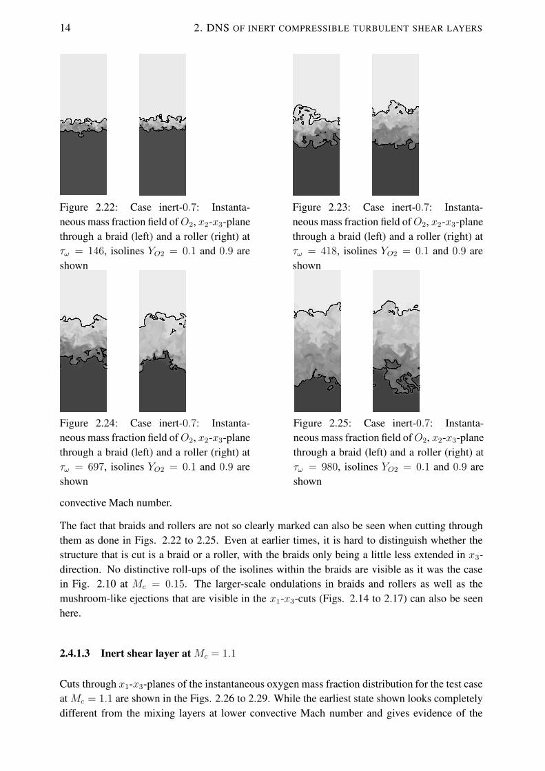
14 2. DNS OF INERT COMPRESSIBLE TURBULENT SHEAR LAYERS
Figure 2.22: Case inert-0.7: Instanta-neous mass fraction field ofO2, x2-x3-planethrough a braid (left) and a roller (right) atτω = 146, isolines YO2 = 0.1 and 0.9 areshown
Figure 2.23: Case inert-0.7: Instanta-neous mass fraction field ofO2, x2-x3-planethrough a braid (left) and a roller (right) atτω = 418, isolines YO2 = 0.1 and 0.9 areshown
Figure 2.24: Case inert-0.7: Instanta-neous mass fraction field ofO2, x2-x3-planethrough a braid (left) and a roller (right) atτω = 697, isolines YO2 = 0.1 and 0.9 areshown
Figure 2.25: Case inert-0.7: Instanta-neous mass fraction field ofO2, x2-x3-planethrough a braid (left) and a roller (right) atτω = 980, isolines YO2 = 0.1 and 0.9 areshown
convective Mach number.
The fact that braids and rollers are not so clearly marked can also be seen when cutting throughthem as done in Figs. 2.22 to 2.25. Even at earlier times, it is hard to distinguish whether thestructure that is cut is a braid or a roller, with the braids only being a little less extended in x3-direction. No distinctive roll-ups of the isolines within the braids are visible as it was the casein Fig. 2.10 at Mc = 0.15. The larger-scale ondulations in braids and rollers as well as themushroom-like ejections that are visible in the x1-x3-cuts (Figs. 2.14 to 2.17) can also be seenhere.
2.4.1.3 Inert shear layer at Mc = 1.1
Cuts through x1-x3-planes of the instantaneous oxygen mass fraction distribution for the test caseat Mc = 1.1 are shown in the Figs. 2.26 to 2.29. While the earliest state shown looks completelydifferent from the mixing layers at lower convective Mach number and gives evidence of the
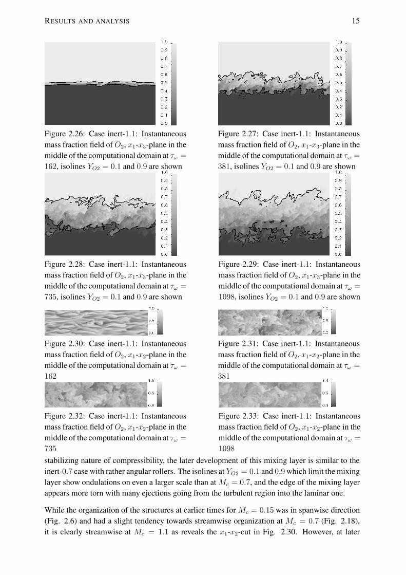
RESULTS AND ANALYSIS 15
Figure 2.26: Case inert-1.1: Instantaneousmass fraction field of O2, x1-x3-plane in themiddle of the computational domain at τω =
162, isolines YO2 = 0.1 and 0.9 are shown
Figure 2.27: Case inert-1.1: Instantaneousmass fraction field of O2, x1-x3-plane in themiddle of the computational domain at τω =
381, isolines YO2 = 0.1 and 0.9 are shown
Figure 2.28: Case inert-1.1: Instantaneousmass fraction field of O2, x1-x3-plane in themiddle of the computational domain at τω =
735, isolines YO2 = 0.1 and 0.9 are shown
Figure 2.29: Case inert-1.1: Instantaneousmass fraction field of O2, x1-x3-plane in themiddle of the computational domain at τω =
1098, isolines YO2 = 0.1 and 0.9 are shown
Figure 2.30: Case inert-1.1: Instantaneousmass fraction field of O2, x1-x2-plane in themiddle of the computational domain at τω =
162
Figure 2.31: Case inert-1.1: Instantaneousmass fraction field of O2, x1-x2-plane in themiddle of the computational domain at τω =
381
Figure 2.32: Case inert-1.1: Instantaneousmass fraction field of O2, x1-x2-plane in themiddle of the computational domain at τω =
735
Figure 2.33: Case inert-1.1: Instantaneousmass fraction field of O2, x1-x2-plane in themiddle of the computational domain at τω =
1098
stabilizing nature of compressibility, the later development of this mixing layer is similar to theinert-0.7 case with rather angular rollers. The isolines at YO2 = 0.1 and 0.9 which limit the mixinglayer show ondulations on even a larger scale than at Mc = 0.7, and the edge of the mixing layerappears more torn with many ejections going from the turbulent region into the laminar one.
While the organization of the structures at earlier times for Mc = 0.15 was in spanwise direction(Fig. 2.6) and had a slight tendency towards streamwise organization at Mc = 0.7 (Fig. 2.18),it is clearly streamwise at Mc = 1.1 as reveals the x1-x2-cut in Fig. 2.30. However, at later
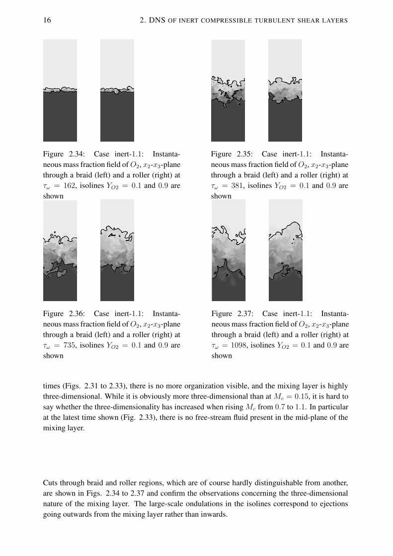
16 2. DNS OF INERT COMPRESSIBLE TURBULENT SHEAR LAYERS
Figure 2.34: Case inert-1.1: Instanta-neous mass fraction field ofO2, x2-x3-planethrough a braid (left) and a roller (right) atτω = 162, isolines YO2 = 0.1 and 0.9 areshown
Figure 2.35: Case inert-1.1: Instanta-neous mass fraction field ofO2, x2-x3-planethrough a braid (left) and a roller (right) atτω = 381, isolines YO2 = 0.1 and 0.9 areshown
Figure 2.36: Case inert-1.1: Instanta-neous mass fraction field ofO2, x2-x3-planethrough a braid (left) and a roller (right) atτω = 735, isolines YO2 = 0.1 and 0.9 areshown
Figure 2.37: Case inert-1.1: Instanta-neous mass fraction field ofO2, x2-x3-planethrough a braid (left) and a roller (right) atτω = 1098, isolines YO2 = 0.1 and 0.9 areshown
times (Figs. 2.31 to 2.33), there is no more organization visible, and the mixing layer is highlythree-dimensional. While it is obviously more three-dimensional than at Mc = 0.15, it is hard tosay whether the three-dimensionality has increased when rising Mc from 0.7 to 1.1. In particularat the latest time shown (Fig. 2.33), there is no free-stream fluid present in the mid-plane of themixing layer.
Cuts through braid and roller regions, which are of course hardly distinguishable from another,are shown in Figs. 2.34 to 2.37 and confirm the observations concerning the three-dimensionalnature of the mixing layer. The large-scale ondulations in the isolines correspond to ejectionsgoing outwards from the mixing layer rather than inwards.
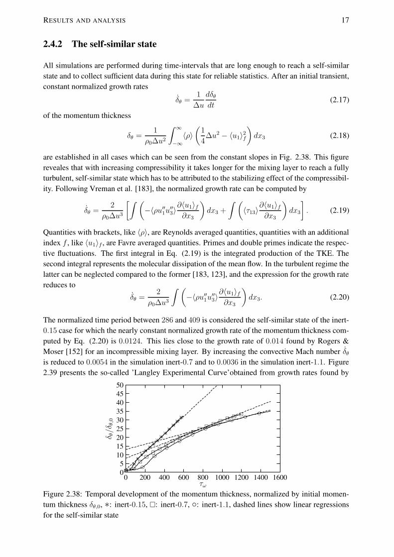
RESULTS AND ANALYSIS 17
2.4.2 The self-similar state
All simulations are performed during time-intervals that are long enough to reach a self-similarstate and to collect sufficient data during this state for reliable statistics. After an initial transient,constant normalized growth rates
δθ =1
∆u
dδθdt
(2.17)
of the momentum thickness
δθ =1
ρ0∆u2
∫ ∞
−∞〈ρ〉(
1
4∆u2 − 〈u1〉2f
)dx3 (2.18)
are established in all cases which can be seen from the constant slopes in Fig. 2.38. This figurereveales that with increasing compressibility it takes longer for the mixing layer to reach a fullyturbulent, self-similar state which has to be attributed to the stabilizing effect of the compressibil-ity. Following Vreman et al. [183], the normalized growth rate can be computed by
δθ =2
ρ0∆u3
[∫ (−〈ρu′′1u′′3〉
∂〈u1〉f∂x3
)dx3 +
∫ (〈τ13〉
∂〈u1〉f∂x3
)dx3
]. (2.19)
Quantities with brackets, like 〈ρ〉, are Reynolds averaged quantities, quantities with an additionalindex f , like 〈u1〉f , are Favre averaged quantities. Primes and double primes indicate the respec-tive fluctuations. The first integral in Eq. (2.19) is the integrated production of the TKE. Thesecond integral represents the molecular dissipation of the mean flow. In the turbulent regime thelatter can be neglected compared to the former [183, 123], and the expression for the growth ratereduces to
δθ =2
ρ0∆u3
∫ (−〈ρu′′1u′′3〉
∂〈u1〉f∂x3
)dx3. (2.20)
The normalized time period between 286 and 409 is considered the self-similar state of the inert-0.15 case for which the nearly constant normalized growth rate of the momentum thickness com-puted by Eq. (2.20) is 0.0124. This lies close to the growth rate of 0.014 found by Rogers &Moser [152] for an incompressible mixing layer. By increasing the convective Mach number δθis reduced to 0.0054 in the simulation inert-0.7 and to 0.0036 in the simulation inert-1.1. Figure2.39 presents the so-called ’Langley Experimental Curve’obtained from growth rates found by
τω
δ θ/δθ,0
16001400120010008006004002000
50454035302520151050
Figure 2.38: Temporal development of the momentum thickness, normalized by initial momen-tum thickness δθ,0, ∗: inert-0.15, �: inert-0.7, ◦: inert-1.1, dashed lines show linear regressionsfor the self-similar state

18 2. DNS OF INERT COMPRESSIBLE TURBULENT SHEAR LAYERS
Mc
δ/δ inc
1.61.41.210.80.60.40.20
10.9
0.8
0.7
0.6
0.5
0.4
0.3
0.2
Figure 2.39: Dependence of shear layer growth rate on Mc: solid line: Langley curve, +: De-bisschop & Bonnet [36], ×: Samimy & Elliot [155], ∗: Chambres, Barre & Bonnet [25], �:Papamoschou & Roshko [126], �: Clemens & Mungal [27], ◦: Hall, Dimotakis & Rosemann[71], •: Pantano & Sarkar [123],4: Present DNS
early air-air shear layer experimentalists along with various other experimental results, the DNSresults of Pantano & Sarkar [123] and the present DNS results. Our results are lying within theregion where other experiments are situated. However, they are below the DNS results of Pan-tano & Sarkar who did similar computations to the present ones. This fact is commented on inthe course of this section.
The beginning and the end of the self-similar states, along with the corresponding Reynoldsnumbers
Reω =∆u ρ0 δω
µ0(2.21)
are summarized in table 2.2. They are based on the instantaneous vorticity thickness
δω =∆u
(∂〈u1〉f/∂x3)max. (2.22)
The peak values of the micro-scale Reynolds number,
Reλ = 2k
√5ρ
νε, (2.23)
where ν is the kinematic viscosity, k the TKE and ε its dissipation rate (see Eq. (2.27)) are alsogiven in table 2.2. This Reynolds number is based on the Taylor micro-scale
λ =
√10ρνk
ε. (2.24)
The initial ratio between the vorticity thickness and the momentum thickness is 4.0 which is dueto the initialization of the vorticity by a hyperbolic-tangent profile. It increases during the initialdevelopment to values around 5.5 for all test cases but relaxes back during the self-similar stateto approximately the initial value.
A normalization by the variables δω, ρ0 and ∆u allows to verify if a truly self-similar state isreached by following the temporal development of profiles which are spatially averaged over thetwo homogeneous directions. Figures 2.40 to 2.42 show profiles of the Reynolds shear stress
〈ρ〉R13 = 〈ρu′′1u′′3〉 (2.25)

RESULTS AND ANALYSIS 19
Table 2.2: Dimensionless times and Reynolds numbers at the beginning (index: B) and end (in-dex: E) of the self-similar state
τω,B τω,E Reω,B Reω,E Reλ,B Reλ,E
inert-0.15 286 409 11540 13410 122 144inert-0.7 626 980 15370 18014 100 105inert-1.1 1023 1305 18586 22353 85 90
at different times for the three inert test cases, respectively. The relaxation to a self-similar stateis visible. Consequently, a temporal averaging of the appropriately normalized profiles over thisstate is possible. A similar collapse can be observed for other profiles, e.g. those of the otherReynolds stresses, the TKE, the dissipation rate of the TKE or the variance of the mass fractionsand their dissipation rate.
In Figs. 2.43 to 2.47, the mean streamwise velocity and the rms velocities computed from theturbulent stress tensor
〈ρ〉Rij = 〈ρu′′i u′′j 〉 (2.26)
of case inert-0.15 are shown in comparison with other DNS and experimental values. The profilesof the numerical simulations are averaged both spatially over the two homogeneous directions
x3/δω
〈u′′ 1u′′ 3〉 f/
(∆u
2)
10.50-0.5-1
0.002
0
-0.002
-0.004
-0.006
-0.008
-0.01
-0.012
-0.014
Figure 2.40: Case inert-0.15: Spatially av-eraged profiles of the Reynolds shear stressR13 at different times, +: τω = 83, ×:τω = 123, ∗: τω = 164, �: τω = 204,�: τω = 245, ◦: τω = 286, •: τω = 327,4:τω = 368
x3/δω
〈u′′ 1u′′ 3〉 f/
(∆u
2)
10.50-0.5-1
0.001
0
-0.001
-0.002
-0.003
-0.004
-0.005
-0.006
-0.007
Figure 2.41: Case inert-0.7: Spatially aver-aged profiles of the Reynolds shear stressR13 at different times, +: τω = 390, ×:τω = 474, ∗: τω = 557, �: τω = 640,�: τω = 725, ◦: τω = 809, •: τω = 866,4:τω = 923
x3/δω
〈u′′ 1u′′ 3〉 f/
(∆u
2)
10.50-0.5-1
0.001
0
-0.001
-0.002
-0.003
-0.004
-0.005
-0.006
-0.007
Figure 2.42: Case inert-1.1: Spatially aver-aged profiles of the Reynolds shear stressR13 at different times, +: τω = 735, ×:τω = 807, ∗: τω = 878, �: τω = 949, �:τω = 1023, ◦: τω = 1098, •: τω = 1174,4: τω = 1248

20 2. DNS OF INERT COMPRESSIBLE TURBULENT SHEAR LAYERS
x3/δω
〈u〉/
∆u
1.510.50-0.5-1-1.5
0.6
0.4
0.2
0
-0.2
-0.4
-0.6
Figure 2.43: Streamwise velocity, solidline: inert-0.15, dashed line: DNS Pantano& Sarkar Mc = 0.3 [123], [152], +: Exper-iments Bell & Mehta [7], ×: ExperimentsSpencer & Jones [172]
x3/δω
√〈u′′ 1u′′ 1〉 f/∆
u
1.510.50-0.5-1-1.5
0.20.180.160.140.12
0.10.080.060.040.02
0
Figure 2.44: Streamwise rms velocity, solidline: inert-0.15, dashed line: DNS Pantano& Sarkar Mc = 0.3 [123], dotted line: DNSRogers & Moser, [152], +: ExperimentsBell & Mehta [7], ×: Experiments Spencer& Jones [172]
x3/δω
√〈u′′ 2u′′ 2〉 f/∆
u
1.510.50-0.5-1-1.5
0.16
0.14
0.12
0.1
0.08
0.06
0.04
0.02
0
Figure 2.45: Spanwise rms velocity, curvesas in Fig. 2.44
x3/δω
√〈u′′ 3u′′ 3〉 f/∆
u
1.510.50-0.5-1-1.5
0.16
0.14
0.12
0.1
0.08
0.06
0.04
0.02
0
Figure 2.46: Transverse rms velocity,curves as in Fig. 2.44
x3/δω
√|〈u′′ 1u′′ 3〉 f|/∆
u
1.510.50-0.5-1-1.5
0.12
0.1
0.08
0.06
0.04
0.02
0
Figure 2.47: Velocity computed fromReynolds shear stress, curves as in Fig. 2.44
and temporally over the self-similar state. This is the case for all profiles in the following ifnot mentioned otherwise. In general, the agreement of the present profiles with the others isgood which verifies the computation. However, it is interesting to note that the width of the rmsvelocity profiles varies which can be due to different initial developments in the time elapseduntil self-similarity is reached. While Rogers & Moser [152] initialized their simulation witha turbulent field from a previous boundary layer DNS, the present DNS were initialized withlaminar profiles and broadband fluctuations in the velocity components only. Pantano & Sarkar[123] used similar broadband fluctuations in the velocity components but superimposed additionalpressure and density fluctuations. Little unsymmetries in the profiles of the present simulationmay be attributed to the density ratio of 1.14 between oxygen in the upper stream and nitrogen inthe lower one.
Most of the rms velocity profiles of the current DNS have a somewhat lower peak than the DNSprofiles of Rogers & Moser [152] as well as the ones of Pantano & Sarkar [123]. One reasonmight be that the size of the present computation domain is more than four times larger in all

RESULTS AND ANALYSIS 21
directions than the simulation of Rogers & Moser and 1.5 times larger in the streamwise andspanwise directions and 2.25 times larger in transverse direction than the one of Pantano & Sarkar.Therefore, the present simulation probably captures the relaxation towards a self-similar state (seeFig. 2.40) more completely than the ones with the smaller domains. This conclusion is drawnfrom our simulations in shorter domains (not documented here) which led to higher peak valuesin the rms velocity profiles.
Figure 2.48 shows the most important terms in the transport equation of TKE k for case inert-0.15,
∂ (〈ρ〉k)
∂t+∂ (〈ρ〉〈uk〉fk)
∂xk= P + ε + T + Π + Σ (2.27)
with the production P , the dissipation rate ε, the transport T , the pressure dilatation Π and themass flux coupling term Σ. The agreement between the present DNS and the simulations ofPantano & Sarkar as well as Rogers & Moser is good taking into account the previously men-tioned reasons for discrepancies. Equation (2.27) is obtained from the transport equation for theReynolds stresses,
∂〈ρ〉Rij
∂t+∂ (〈ρ〉〈uk〉fRij)
∂xk= Pij + εij + Tij + Πij + Σij, (2.28)
by contracting the indices (k = 0.5Rkk). In Eq. (2.28), the production term is
Pij = −〈ρ〉(Rik
∂〈uj〉f∂xk
+Rjk∂〈ui〉f∂xk
), (2.29)
the dissipation rate,
εij = −〈τ ′jk∂u′′i∂xk
+ τ ′ik∂u′′j∂xk〉, (2.30)
the transport by velocity and pressure fluctuations as well as viscous effects,
Tij = − ∂
∂xk〈ρu′′i u′′ju′′k + p′u′iδjk + p′u′jδik − τ ′jku′′i − τ ′iku′′j 〉, (2.31)
the pressure-strain term,
Πij = 〈p′(∂u′′i∂xj
+∂u′′j∂xi
)〉 (2.32)
x3/δθ43210-1-2-3-4
0.0025
0.002
0.0015
0.001
0.0005
0
-0.0005
-0.001
-0.0015
Figure 2.48: Turbulent kinetic energy budget, +: production, ×: transport, ∗: dissipation, nor-malized by ∆u3δθ, solid lines: inert-0.15, dashed lines: DNS Pantano & Sarkar Mc = 0.3 [123],dotted line: DNS Rogers & Moser, [152]
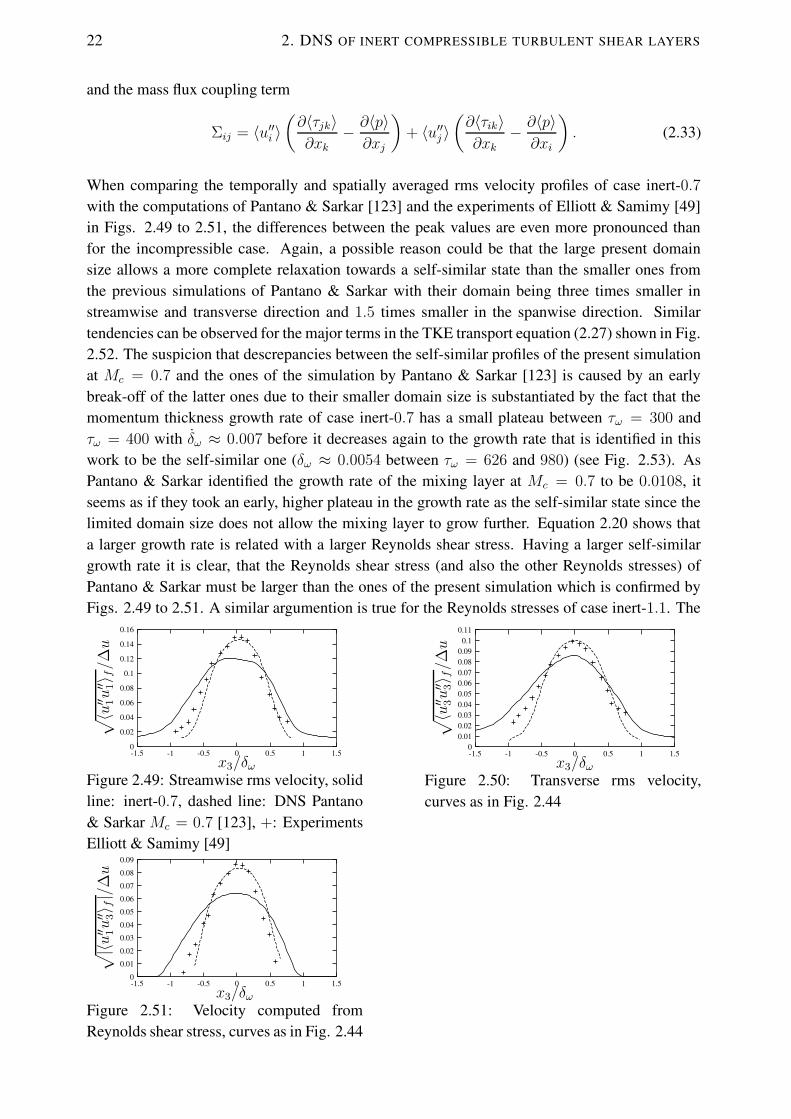
22 2. DNS OF INERT COMPRESSIBLE TURBULENT SHEAR LAYERS
and the mass flux coupling term
Σij = 〈u′′i 〉(∂〈τjk〉∂xk
− ∂〈p〉∂xj
)+ 〈u′′j 〉
(∂〈τik〉∂xk
− ∂〈p〉∂xi
). (2.33)
When comparing the temporally and spatially averaged rms velocity profiles of case inert-0.7with the computations of Pantano & Sarkar [123] and the experiments of Elliott & Samimy [49]in Figs. 2.49 to 2.51, the differences between the peak values are even more pronounced thanfor the incompressible case. Again, a possible reason could be that the large present domainsize allows a more complete relaxation towards a self-similar state than the smaller ones fromthe previous simulations of Pantano & Sarkar with their domain being three times smaller instreamwise and transverse direction and 1.5 times smaller in the spanwise direction. Similartendencies can be observed for the major terms in the TKE transport equation (2.27) shown in Fig.2.52. The suspicion that descrepancies between the self-similar profiles of the present simulationat Mc = 0.7 and the ones of the simulation by Pantano & Sarkar [123] is caused by an earlybreak-off of the latter ones due to their smaller domain size is substantiated by the fact that themomentum thickness growth rate of case inert-0.7 has a small plateau between τω = 300 andτω = 400 with δω ≈ 0.007 before it decreases again to the growth rate that is identified in thiswork to be the self-similar one (δω ≈ 0.0054 between τω = 626 and 980) (see Fig. 2.53). AsPantano & Sarkar identified the growth rate of the mixing layer at Mc = 0.7 to be 0.0108, itseems as if they took an early, higher plateau in the growth rate as the self-similar state since thelimited domain size does not allow the mixing layer to grow further. Equation 2.20 shows thata larger growth rate is related with a larger Reynolds shear stress. Having a larger self-similargrowth rate it is clear, that the Reynolds shear stress (and also the other Reynolds stresses) ofPantano & Sarkar must be larger than the ones of the present simulation which is confirmed byFigs. 2.49 to 2.51. A similar argumention is true for the Reynolds stresses of case inert-1.1. The
x3/δω
√〈u′′ 1u′′ 1〉 f/∆
u
1.510.50-0.5-1-1.5
0.16
0.14
0.12
0.1
0.08
0.06
0.04
0.02
0
Figure 2.49: Streamwise rms velocity, solidline: inert-0.7, dashed line: DNS Pantano& Sarkar Mc = 0.7 [123], +: ExperimentsElliott & Samimy [49]
x3/δω
√〈u′′ 3u′′ 3〉 f/∆
u
1.510.50-0.5-1-1.5
0.110.1
0.090.080.070.060.050.040.030.020.01
0
Figure 2.50: Transverse rms velocity,curves as in Fig. 2.44
x3/δω
√|〈u′′ 1u′′ 3〉 f|/∆
u
1.510.50-0.5-1-1.5
0.09
0.08
0.07
0.06
0.05
0.04
0.03
0.02
0.01
0
Figure 2.51: Velocity computed fromReynolds shear stress, curves as in Fig. 2.44

RESULTS AND ANALYSIS 23
x3/δθ43210-1-2-3-4
0.002
0.0015
0.001
0.0005
0
-0.0005
-0.001
-0.0015
Figure 2.52: Turbulent kinetic energy bud-get, +: production, ×: transport, ∗: dissi-pation, normalized by ∆u3/δθ, solid lines:inert-0.7, dashed lines: DNS Pantano &Sarkar Mc = 0.7 [123]
x3/δω
δ θ
16001400120010008006004002000
0.018
0.016
0.014
0.012
0.01
0.008
0.006
0.004
0.002
0
Figure 2.53: Dimensionless momentumthickness growth rate of the inert-0.7 case,computed with Eq. (2.20)
x3/δθ43210-1-2-3-4
0.001
0.0005
0
-0.0005
-0.001
-0.0015
Figure 2.54: Turbulent kinetic energy bud-get, +: production, ×: transport, ∗: dissi-pation, normalized by ∆u3/δθ, solid lines:inert-1.1, dashed lines: DNS Pantano &Sarkar Mc = 1.1 [123]
most important terms of the TKE budget equation for this test case are shown in Fig. 2.54 incomparison with the results of Pantano & Sarkar [123] which are again larger than the presentresults.
2.4.3 Check of resolution, domain sizes and filtering
In order to verify the accuracy of the results, resolution and domain sizes are checked. All simu-lations are well resolved with a minimal Kolmogorov length
lk =
(〈ν〉3〈ρ〉ε
)1/4
(2.34)
of 0.32∆x3 for case inert-0.15, 0.44∆x3 for case inert-0.7 and 0.58∆x3 for case inert-1.1 duringthe self-similar state. These resolutions are fine enough to accurately capture most of the dis-sipation (cf. Sect. 2.4.4.1) and therefore adequate for DNS [117]. As the Schmidt numbers ofgases are smaller than 1, no resolution problems concerning the scalar fields are expected, either.Various spectra, which are dealt with in Sections 2.4.4.1 and 2.4.4.2, show no accumulation ofenergy at the highest wavenumbers as it would be the case for an under-resolved simulation.
The appropriateness of the domain size in the periodic directions is checked by computing two-point correlations of the velocity components and the species mass fraction. The two-point cor-
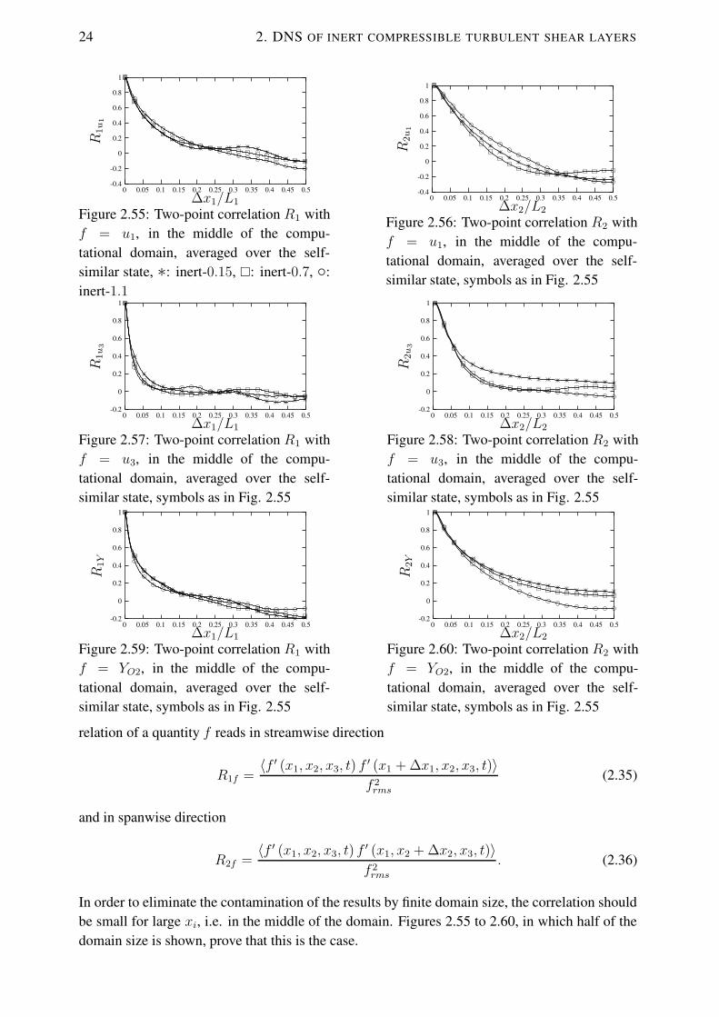
24 2. DNS OF INERT COMPRESSIBLE TURBULENT SHEAR LAYERS
∆x1/L1
R1u
1
0.50.450.40.350.30.250.20.150.10.050
1
0.8
0.6
0.4
0.2
0
-0.2
-0.4
Figure 2.55: Two-point correlation R1 withf = u1, in the middle of the compu-tational domain, averaged over the self-similar state, ∗: inert-0.15, �: inert-0.7, ◦:inert-1.1
∆x2/L2
R2u
1
0.50.450.40.350.30.250.20.150.10.050
1
0.8
0.6
0.4
0.2
0
-0.2
-0.4
Figure 2.56: Two-point correlation R2 withf = u1, in the middle of the compu-tational domain, averaged over the self-similar state, symbols as in Fig. 2.55
∆x1/L1
R1u
3
0.50.450.40.350.30.250.20.150.10.050
1
0.8
0.6
0.4
0.2
0
-0.2
Figure 2.57: Two-point correlation R1 withf = u3, in the middle of the compu-tational domain, averaged over the self-similar state, symbols as in Fig. 2.55
∆x2/L2
R2u
30.50.450.40.350.30.250.20.150.10.050
1
0.8
0.6
0.4
0.2
0
-0.2
Figure 2.58: Two-point correlation R2 withf = u3, in the middle of the compu-tational domain, averaged over the self-similar state, symbols as in Fig. 2.55
∆x1/L1
R1Y
0.50.450.40.350.30.250.20.150.10.050
1
0.8
0.6
0.4
0.2
0
-0.2
Figure 2.59: Two-point correlation R1 withf = YO2, in the middle of the compu-tational domain, averaged over the self-similar state, symbols as in Fig. 2.55
∆x2/L2
R2Y
0.50.450.40.350.30.250.20.150.10.050
1
0.8
0.6
0.4
0.2
0
-0.2
Figure 2.60: Two-point correlation R2 withf = YO2, in the middle of the compu-tational domain, averaged over the self-similar state, symbols as in Fig. 2.55
relation of a quantity f reads in streamwise direction
R1f =〈f ′ (x1, x2, x3, t) f
′ (x1 + ∆x1, x2, x3, t)〉f 2rms
(2.35)
and in spanwise direction
R2f =〈f ′ (x1, x2, x3, t) f
′ (x1, x2 + ∆x2, x3, t)〉f 2rms
. (2.36)
In order to eliminate the contamination of the results by finite domain size, the correlation shouldbe small for large xi, i.e. in the middle of the domain. Figures 2.55 to 2.60, in which half of thedomain size is shown, prove that this is the case.
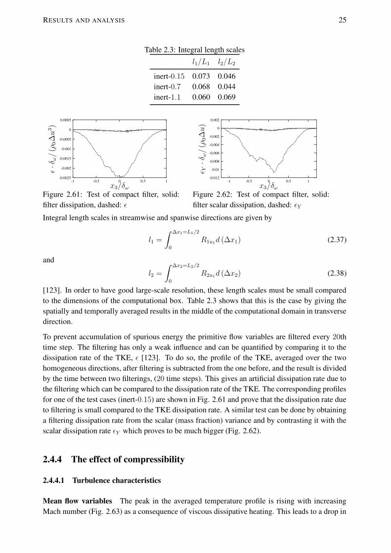
RESULTS AND ANALYSIS 25
Table 2.3: Integral length scalesl1/L1 l2/L2
inert-0.15 0.073 0.046inert-0.7 0.068 0.044inert-1.1 0.060 0.069
x3/δω
ε·δ
ω/
(ρ0∆u
3)
10.50-0.5-1
0.0005
0
-0.0005
-0.001
-0.0015
-0.002
-0.0025
Figure 2.61: Test of compact filter, solid:filter dissipation, dashed: ε
x3/δω
ε Y·δ
ω/
(ρ0∆u
)
10.50-0.5-1
0.002
0
-0.002
-0.004
-0.006
-0.008
-0.01
-0.012
Figure 2.62: Test of compact filter, solid:filter scalar dissipation, dashed: εY
Integral length scales in streamwise and spanwise directions are given by
l1 =
∫ ∆x1=L1/2
0
R1u1d (∆x1) (2.37)
and
l2 =
∫ ∆x2=L2/2
0
R2u1d (∆x2) (2.38)
[123]. In order to have good large-scale resolution, these length scales must be small comparedto the dimensions of the computational box. Table 2.3 shows that this is the case by giving thespatially and temporally averaged results in the middle of the computational domain in transversedirection.
To prevent accumulation of spurious energy the primitive flow variables are filtered every 20thtime step. The filtering has only a weak influence and can be quantified by comparing it to thedissipation rate of the TKE, ε [123]. To do so, the profile of the TKE, averaged over the twohomogeneous directions, after filtering is subtracted from the one before, and the result is dividedby the time between two filterings, (20 time steps). This gives an artificial dissipation rate due tothe filtering which can be compared to the dissipation rate of the TKE. The corresponding profilesfor one of the test cases (inert-0.15) are shown in Fig. 2.61 and prove that the dissipation rate dueto filtering is small compared to the TKE dissipation rate. A similar test can be done by obtaininga filtering dissipation rate from the scalar (mass fraction) variance and by contrasting it with thescalar dissipation rate εY which proves to be much bigger (Fig. 2.62).
2.4.4 The effect of compressibility
2.4.4.1 Turbulence characteristics
Mean flow variables The peak in the averaged temperature profile is rising with increasingMach number (Fig. 2.63) as a consequence of viscous dissipative heating. This leads to a drop in

26 2. DNS OF INERT COMPRESSIBLE TURBULENT SHEAR LAYERS
x3/δω
〈T〉/T
0
10.50-0.5-1
1.14
1.12
1.1
1.08
1.06
1.04
1.02
1
Figure 2.63: Averaged temperature, nor-malized by T0 = 0.5 (T1 + T2), ∗: inert-0.15, �: inert-0.7, ◦: inert-1.1
x3/δω
〈ρ〉/ρ
0
10.50-0.5-1
1.1
1.05
1
0.95
0.9
0.85
Figure 2.64: Averaged density, normalizedby ρ0, symbols as in Fig. 2.63
x3/δω
〈p〉/
(ρ0∆u
2)
10.50-0.5-1
8
7
6
5
4
3
2
1
0
Figure 2.65: Averaged pressure, normalizedby ρ0∆u2, symbols as in Fig. 2.63
x3/δω〈u〉 f/∆
u
10.50-0.5-1
0.50.40.30.20.1
0-0.1-0.2-0.3-0.4-0.5
Figure 2.66: Favre averaged streamwise ve-locity, normalized by ∆u, symbols as inFig. 2.63
the averaged density (Fig. 2.64). The averaged pressure normalized by ρ0∆u2 is nearly constantacross the shear layer (Fig. 2.65) and drops with increasing Mc. Multiplying its value by γM 2
c
respectively, gives the same constant, 0.25, for all Mc which demonstrates that the pressure dropis by γM2
c . Figure 2.66 shows the Favre averaged streamwise velocity. The differences betweenthe cases with the various convective Mach numbers are small.
Reynolds stresses, turbulent kinetic energy and anisotropies Figures 2.67 to 2.70 show theaveraged Reynolds stresses of the three test cases. They are strongly anisotropic with the stream-wise stress being the biggest, followed by the spanwise and then the transverse one. The mag-nitude of the Reynolds shear stress is even smaller. It can be seen that all, the normal stressesand the shear stress, reduce when increasing the convective Mach number. The turbulent kineticenergy in Fig. 2.71 shows the same behaviour. The reduction of R22, R33 and R13 is in agreementwith various experiments [36, 49, 68] and DNS [63, 123]. Concerning the streamwise ReynoldsstressR11, different results can be found: While some experiments and DNS [63, 68] find its peakto be independent of the convective Mach number, others [49, 123] notice a decrease which is inagreement with our results.
x3/δω
〈ρ〉R
11/
(ρ0∆u
2)
10.50-0.5-1
0.03
0.025
0.02
0.015
0.01
0.005
0
Figure 2.67: Reynolds stress 〈ρ〉R11, nor-malized by ρ0∆u2, curves as in Fig. 2.63
x3/δω
〈ρ〉R
22/
(ρ0∆u
2)
10.50-0.5-1
0.016
0.014
0.012
0.01
0.008
0.006
0.004
0.002
0
Figure 2.68: Reynolds stress 〈ρ〉R22, nor-malized by ρ0∆u2, curves as in Fig. 2.63

RESULTS AND ANALYSIS 27
x3/δω
〈ρ〉R
33/
(ρ0∆u
2)
10.50-0.5-1
0.016
0.014
0.012
0.01
0.008
0.006
0.004
0.002
0
Figure 2.69: Reynolds stress 〈ρ〉R33, nor-malized by ρ0∆u2, curves as in Fig. 2.63
x3/δω
〈ρ〉R
13/
(ρ0∆u
2)
10.50-0.5-1
0.0010
-0.001-0.002-0.003-0.004-0.005-0.006-0.007-0.008-0.009
-0.01
Figure 2.70: Reynolds stress 〈ρ〉R13, nor-malized by ρ0∆u2, curves as in Fig. 2.63
x3/δω
〈ρ〉k/
(ρ0∆u
2)
10.50-0.5-1
0.03
0.025
0.02
0.015
0.01
0.005
0
Figure 2.71: Turbulent kinetic energy 〈ρ〉k,normalized by ρ0∆u2, curves as in Fig.2.63The similar behaviour of the normal Reynolds stresses and the shear Reynolds stress with increas-ing convective Mach number makes the shear stress anisotropy parameter
b13 =〈u′′1u′′3〉f
2k(2.39)
nearly independent of the convective Mach number (Fig. 2.72) which was also noticed by Vremanet al. [183]. The anisotropy parameters of the normal Reynolds stress components,
bij =〈u′′i u′′j 〉f
2k− 1
3δij, with i = j (2.40)
x3/δω
b 13
10.50-0.5-1
0.15
0.1
0.05
0
-0.05
-0.1
-0.15
-0.2
Figure 2.72: Reynolds shear stressanisotropy, b13, curves as in Fig. 2.63
x3/δω
b 11
10.50-0.5-1
0.20.180.160.140.12
0.10.080.060.040.02
0
Figure 2.73: Streamwise Reynolds stressanisotropy, b11, curves as in Fig. 2.63
x3/δω
b 22
10.50-0.5-1
0
-0.05
-0.1
-0.15
-0.2
-0.25
-0.3
-0.35
Figure 2.74: Spanwise Reynolds stressanisotropy, b22, curves as in Fig. 2.63
x3/δω
b 33
10.50-0.5-1
0.25
0.2
0.15
0.1
0.05
0
-0.05
-0.1
-0.15
Figure 2.75: Transverse Reynolds stressanisotropy, b33, curves as in Fig. 2.63

28 2. DNS OF INERT COMPRESSIBLE TURBULENT SHEAR LAYERS
are also nearly independent of Mc (Figs. 2.73 to 2.75) which corresponds to the results of [123].However, there are different statements concerning the consequences of compressibility with re-spect to the anisotropy of the Reynolds stresses in free shear flows, e.g. [183] (increase of trans-verse anisotropy, no effect on shear stress anisotropy) or [63] (increase of transverse anisotropy,decrease of shear stress anisotropy). Pantano & Sarkar [123] found in their DNS of turbulentcompressible shear layers that all diagonal components of the Reynolds stresses, as well as theReynolds shear stress decrease with increasing convective Mach number. They also showedin agreement with experiments [6, 155] that compressibility has only a weak influence on theanisotropy of the Reynolds stresses at least in the full turbulent, self-similar state and the Machnumber range considered. In addition, Pantano & Sarkar [123] noticed that during the initialtransient evolution, the anisotropy tensor is strongly affected by the convective Mach number Mc
which could be a possible explanation for the discrepancies of earlier experiments and simula-tions.
Reynolds stress transport equations Figures 2.76 to 2.83 show the major terms of the trans-port equation of the Reqnolds stresses (2.28). The biggest source term in the R11 equation is theTKE production, the biggest sinks are the dissipation rate and the pressure-strain rate. The latterone acts to redistribute energy from the streamwise component of the Reynolds stresses, R11,to the spanwise and transverse components, R22 and R33. The pressure-strain rate is the majorsource term in the transport equations of these Reynolds stress components. Contrarily toR11, the
x3/δω10.50-0.5-1
0.0160.0140.0120.01
0.0080.0060.0040.002
0-0.002-0.004
Figure 2.76: Budget of R11, normalized by ρ0∆u3/δω, symbols as in Fig. 2.63, solid: production,dashed: dissipation rate
x3/δω10.50-0.5-1
0.004
0.002
0
-0.002
-0.004
-0.006
-0.008
-0.01
Figure 2.77: Budget of R11, normalized by ρ0∆u3/δω, symbols as in Fig. 2.63, solid: pressure-strain rate, dashed: turbulent transport

RESULTS AND ANALYSIS 29
x3/δω10.50-0.5-1
0.0005
0
-0.0005
-0.001
-0.0015
-0.002
-0.0025
-0.003
-0.0035
Figure 2.78: Budget of R22, normalized by ρ0∆u3/δω, symbols as in Fig. 2.63, solid: production,dashed: dissipation rate
x3/δω10.50-0.5-1
0.005
0.004
0.003
0.002
0.001
0
-0.001
-0.002
Figure 2.79: Budget of R22, normalized by ρ0∆u3/δω, symbols as in Fig. 2.63, solid: pressure-strain rate, dashed: turbulent transport
production term of R22 and R33 is zero and no energy is coming directly from the mean flow. Therole of the turbulent transport is the same in all diagonal Reynolds stresses: It takes energy awayfrom the central region and transports it to the edges of the shear layer. The dissipation rates havenearly the same magnitudes in all budgets of the diagonal Reynolds stresses at each convectiveMach number, respectively, which is supported by the argument that for high Reynolds numbersthe turbulence, which is isotropic at small scales, implies isotropic dissipation [183].
One major effect of compressibility is to reduce the production rate of R11. This is a clear con-sequence of the reduced Reynolds shear stress R13 (Fig. 2.70) as it appears as a factor in theproduction rate
P11 = −2R13∂〈u1〉f∂x3
(2.41)
and the Favre averaged velocity profile hardly changes in particular in the center of the shear layer(Fig. 2.66). Pressure-strain rate and turbulent transport of R11 are also decreased with increasingconvective Mach number as is the dissipation rate. This is also the case for R22 and R33. Pantano& Sarkar [123] found the magnitude of ε11 rather independent of Mc and noticed a small decreaseof ε33 which is approximately of the size of the decrease found in this study. Even though ε11 inthe present test cases is not constant, it is shown later that its influence on the shear layer growthrate is small compared to the influence of the pressure-strain rate.
The major source of the Reynolds shear stress R13 is the production and its only major sink thepressure-strain rate (Figs. 2.82 and 2.83). As R13 is negative, the production is negative too and

30 2. DNS OF INERT COMPRESSIBLE TURBULENT SHEAR LAYERS
x3/δω10.50-0.5-1
0.0005
0
-0.0005
-0.001
-0.0015
-0.002
-0.0025
-0.003
-0.0035
Figure 2.80: Budget of R33, normalized by ρ0∆u3/δω, symbols as in Fig. 2.63, solid: production,dashed: dissipation rate
x3/δω10.50-0.5-1
0.0070.0060.0050.0040.0030.0020.001
0-0.001-0.002-0.003
Figure 2.81: Budget of R33, normalized by ρ0∆u3/δω, symbols as in Fig. 2.63, solid: pressure-strain rate, dashed: turbulent transport
the pressure-strain rate is positive. The turbulent transport oscillates around zero (for unknownreasons), and therefore its role is not as clear as for the diagonal Reynolds stresses. The fact thatthe dissipation rate ε13 is approximately zero is consistent with the expected isotropic dissipationat sufficiently high Reynolds numbers. The influence of compressibility on the budget terms ofthe Reynolds shear stress is the same as for the normal Reynolds stresses: In particular the majorones, namely production and pressure-strain rate, are decreased with increasing Mc.
Quantities integrated in the transverse direction are convenient as they are less sensitive to thesample size. They are defined in the following way (using the production P as an example):
P =
∫ ∞
−∞Pdx3 (2.42)
When integrating all budget terms this way, the following set of ordinary differential equations isobtained:
∂〈ρ〉R11
∂t= P11 + Π11 + ε11
∂〈ρ〉R22
∂t= Π22 + ε22
∂〈ρ〉R33
∂t= Π33 + ε33
∂〈ρ〉R13
∂t= P13 + Π13 + ε13
(2.43)

RESULTS AND ANALYSIS 31
x3/δω10.50-0.5-1
0.0025
0
-0.0025
-0.005
-0.0075
-0.01
-0.0125
Figure 2.82: Budget of R13, normalized by ρ0∆u3/δω, symbols as in Fig. 2.63, solid: production,dashed: dissipation rate
x3/δω10.50-0.5-1
0.05
0.04
0.03
0.02
0.01
0
-0.01
Figure 2.83: Budget of R13, normalized by ρ0∆u3/δω, symbols as in Fig. 2.63, solid: pressure-strain rate, dashed: turbulent transport
as terms in divergence form vanish after integration. These or slightly modified equations wherealso used by other authors [183, 63, 123] for similar studies. As shown by Fig. 2.82, the shearstress dissipation can be neglected at all Mc (|ε13| < 0.04
∣∣∣P13
∣∣∣).
Figures 2.84 to 2.86 show the integrated normalized production, pressure-strain and dissipationrate as functions of the convective Mach number. Certain ratios of these terms are found to beindependent of the Mach number and are shown in Fig. 2.87. Freund et al. [63] denoted theseconstant ratios for their annular mixing layer, too. From Fig. 2.87 it can be seen that a reducedgrowth rate at high Mc cannot be explained by an increase in the ratios of pressure-strain andproduction in the budget equation of R11 and R13 as these ratios are nearly constant. This hasalso been pointed out by Vreman et al. [183]. The figure also shows that P13 ≈ 1.28Π11 andΠ13 ≈ −1.13Π11. Neglecting ε13, the budget equation for R13 can be simplified to
∂〈ρ〉R13
∂t= 1.28Π11 − 1.13Π11 = 0.15Π11. (2.44)
This demonstrates that the streamwise pressure-strain rate, Π11 can be directly linked with thetemporal development of the Reynolds shear stress. Any influences of compressibility on Π11 aretherefore not only influencing R11 directly but also via its production rate P11 that is linked withR13 (Eq. (2.41)).

32 2. DNS OF INERT COMPRESSIBLE TURBULENT SHEAR LAYERS
Mc
∣ ∣ ∣Pij
∣ ∣ ∣/(ρ
0∆u
3)
1.21.110.90.80.70.60.50.40.30.20.1
0.014
0.012
0.01
0.008
0.006
0.004
0.002
0
-0.002
Figure 2.84: Production, integrated in trans-verse direction, normalized by ρ0∆u3: +: P11,◦: P22, ∗: P33, �: P13
Mc
∣ ∣ ∣Πij
∣ ∣ ∣/(ρ
0∆u
3)
1.21.110.90.80.70.60.50.40.30.20.1
0.009
0.008
0.007
0.006
0.005
0.004
0.003
0.002
0.001
Figure 2.85: Pressure-strain rate, integrated intransverse direction, normalized by ρ0∆u3: +:Π11, ◦: Π22, ∗: Π33, �: Π13
Mc
|ε ij|/
(ρ0∆u
3)
1.21.110.90.80.70.60.50.40.30.20.1
0.0035
0.003
0.0025
0.002
0.0015
0.001
0.0005
0
Figure 2.86: Dissipation rate, integrated intransverse direction, normalized by ρ0∆u3: +:ε11, ◦: ε22, ∗: ε33, �: ε13
Mc
1.21.110.90.80.70.60.50.40.30.20.1
1.4
1.3
1.2
1.1
1
0.9
0.8
0.7
0.6
Figure 2.87: Ratios of integrated budget terms:+: −Π11/P11, ×: −Π13/P13, ∗: P13/Π11, �:−Π13/Π11
Analysis of the reduced growth rate It is possible to directly explain the growth rate reductionfrom the streamwise Reynolds stress equation by establishing a relation between the pressure-strain rate and the momentum thickness. This was done in similar ways by Freund et al. [63] andPantano & Sarkar [123].
The integrated production rate P11 can be related to the momentum thickness growth rate δθ byusing Eq. (2.20):
P11 = ρ0∆u3δθ. (2.45)
From Fig. 2.86 it can be seen that the factor Kε in
ε11 = −Kερ0∆u3 (2.46)
is not constant in our simulation which differs from the results of Freund et al. [63]. However,later we will show that its variation is of little influence on the growth rate. The exact values ofKε for each Mc are given in table 2.4.
By substituting (2.45) and (2.46) into (2.43),
∂〈ρ〉R11
∂t= ρ0∆u3
(δθ −Kε
)+ Π11 (2.47)
Table 2.4: Values used in the analysis linking momentum thickness growth rate with pressure-strain rate Π11 for the inert test cases
Mc Kε K11 Π11/ (ρ0∆u3)
0.15 3.0845 · 10−3 1.0543 · 10−1 −8.3972 · 10−3
0.7 1.8395 · 10−3 6.2236 · 10−2 −3.4054 · 10−3
1.1 1.2830 · 10−3 3.9643 · 10−2 −2.4020 · 10−3
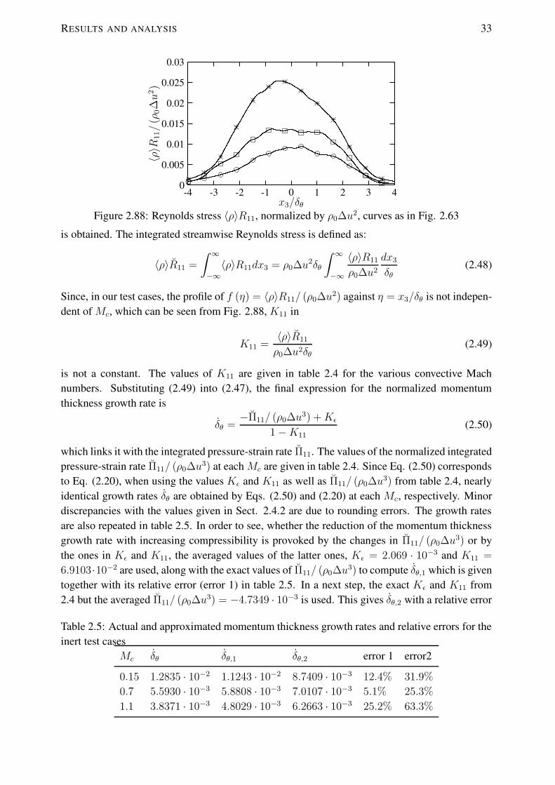
RESULTS AND ANALYSIS 33
x3/δθ
〈ρ〉R
11/
(ρ0∆u
2)
43210-1-2-3-4
0.03
0.025
0.02
0.015
0.01
0.005
0
Figure 2.88: Reynolds stress 〈ρ〉R11, normalized by ρ0∆u2, curves as in Fig. 2.63
is obtained. The integrated streamwise Reynolds stress is defined as:
〈ρ〉R11 =
∫ ∞
−∞〈ρ〉R11dx3 = ρ0∆u2δθ
∫ ∞
−∞
〈ρ〉R11
ρ0∆u2
dx3
δθ(2.48)
Since, in our test cases, the profile of f (η) = 〈ρ〉R11/ (ρ0∆u2) against η = x3/δθ is not indepen-dent of Mc, which can be seen from Fig. 2.88, K11 in
K11 =〈ρ〉R11
ρ0∆u2δθ(2.49)
is not a constant. The values of K11 are given in table 2.4 for the various convective Machnumbers. Substituting (2.49) into (2.47), the final expression for the normalized momentumthickness growth rate is
δθ =−Π11/ (ρ0∆u3) +Kε
1−K11(2.50)
which links it with the integrated pressure-strain rate Π11. The values of the normalized integratedpressure-strain rate Π11/ (ρ0∆u3) at each Mc are given in table 2.4. Since Eq. (2.50) correspondsto Eq. (2.20), when using the values Kε and K11 as well as Π11/ (ρ0∆u3) from table 2.4, nearlyidentical growth rates δθ are obtained by Eqs. (2.50) and (2.20) at each Mc, respectively. Minordiscrepancies with the values given in Sect. 2.4.2 are due to rounding errors. The growth ratesare also repeated in table 2.5. In order to see, whether the reduction of the momentum thicknessgrowth rate with increasing compressibility is provoked by the changes in Π11/ (ρ0∆u3) or bythe ones in Kε and K11, the averaged values of the latter ones, Kε = 2.069 · 10−3 and K11 =
6.9103·10−2 are used, along with the exact values of Π11/ (ρ0∆u3) to compute δθ,1 which is giventogether with its relative error (error 1) in table 2.5. In a next step, the exact Kε and K11 from2.4 but the averaged Π11/ (ρ0∆u3) = −4.7349 · 10−3 is used. This gives δθ,2 with a relative error
Table 2.5: Actual and approximated momentum thickness growth rates and relative errors for theinert test cases
Mc δθ δθ,1 δθ,2 error 1 error2
0.15 1.2835 · 10−2 1.1243 · 10−2 8.7409 · 10−3 12.4% 31.9%
0.7 5.5930 · 10−3 5.8808 · 10−3 7.0107 · 10−3 5.1% 25.3%
1.1 3.8371 · 10−3 4.8029 · 10−3 6.2663 · 10−3 25.2% 63.3%

34 2. DNS OF INERT COMPRESSIBLE TURBULENT SHEAR LAYERS
(error 2) that is given in table 2.5, too. Comparing the errors, one can see that the influence ofthe variation of the pressure-strain rate with compressibility has a much greater influence than thevariation of Kε and K11 which include the influences of dissipation rate and streamwise Reynoldsstress. This is particularly true for the highest Mach number.
Pressure-strain terms There are three, maybe simultaneously occuring possibilities, how thepressure-strain rate
Π11 = 2〈p′∂u′′1
∂x1〉 (2.51)
might be reduced: Either by a reduction of the pressure fluctuations p′, by a reduction of the strainrate fluctuations ∂u′′1/∂x1 or by a reduction of their correlation coefficient. It is demonstrated inthe following as an example for the streamwise component of the pressure-strain rate tensor whichone of these possibilities is the most plausible one.
Figure 2.89 shows the rms value of the pressure fluctuations, Fig. 2.90, the rms value of strainrate fluctuations and Fig. 2.91, the correlation coefficient of both fluctuations,
R (p, ∂u1/∂x1) =〈p′∂u′′1/∂x1〉
prms (∂u1/∂x1)rms. (2.52)
It is visible that the pressure fluctuations reduce much more with increasing compressibility thanthe fluctuations of the strain rate and that the correlation coefficient remains small for all Mc,which suggests that the reduction of the pressure fluctuations is primarily responsible for thereduced pressure-strain rates. This is confirmed by Fig. 2.92 which presents the relative reductionof the integrated rms value of p′, of the integrated rms value of ∂u′′1/∂x1 and the integrated
x3/δω
p rms/
(ρ0∆u
2)
10.50-0.5-1
0.04
0.035
0.03
0.025
0.02
0.015
0.01
0.005
Figure 2.89: Rms value of p′, normalized byρ0∆u2, curves as in Fig. 2.63
x3/δω
(∂u
1/∂x
1) rmsδ ω,0/∆
u
10.50-0.5-1
21.81.61.41.2
10.80.60.40.2
0
Figure 2.90: Rms value of ∂u′′1/∂x1, normal-ized by δω,0/∆u, curves as in Fig. 2.63
x3/δω
R(p,∂u
1/∂x
1)
10.50-0.5-1
0.15
0.1
0.05
0
-0.05
-0.1
-0.15
-0.2
Figure 2.91: Correlation coefficientR (p, ∂u1/∂x1) between pressure and densityfluctuations, curves as in Fig. 2.63
Mc
1.21.110.90.80.70.60.50.40.30.20.1
1
0.9
0.8
0.7
0.6
0.5
0.4
0.3
0.2
0.1
Figure 2.92: Suppression of integrated prms(+), integrated (∂u′′1/∂x1)rms (×) and inte-grated pressure-strain rate |Π11| (∗), normal-ized by the respective incompressible value atMc = 0.15

RESULTS AND ANALYSIS 35
pressure-strain rate |Π11|: The pressure fluctuations are the predominant reason for the reducedpressure-strain rate since they are reduced in a similar manner with increasing Mc. The strain ratefluctuations are also reduced for increasing Mc but to a lesser extent. Similar results are obtainedfor the other components of the pressure-strain rate tensor (not shown). The reduction of thepressure-strain rates with increasing Mc is further investigated in Sect. 2.4.4.1.
TKE transport equation The major terms of the transport equation for the TKE, Eq. (2.27),are shown in Figs. 2.93 and 2.94. The major source term, namely production, is reduced withincreasing Mach number. The turbulent transport acts as a sink in the middle of the shear layer andas a source at its edges. It therefore moves kinetic energy away from the region of highest shear,where it is produced, to regions of less production. The pressure dilatation is very small. Thismeans that the pressure-strain tensor is nearly trace free, and that its major role is to redistributeenergy from the streamwise component of the Reynolds stress to the spanwise and transversecomponents the transport equations of which have no production terms. Figure 2.95 shows theratio of the integrated pressure dilatation term, Π and the production term P against Mc. Itsmagnitude increases with increasing Mc, which is partially due to the reduced production at highMc and remains small in total. The dissipation rate, the major sink in the TKE transport equation,is also reduced by compressibility (Fig. 2.94), however not as much as the production rate. Thiscan be seen from Fig. 2.96 which shows that the magnitude of the ratio of the dissipation ratewith respect to the production increases with increasing Mc.
x3/δω10.50-0.5-1
0.008
0.006
0.004
0.002
0
-0.002
-0.004
-0.006
Figure 2.93: Budget of 〈ρ〉k, normalized by ρ0∆u3/δω, symbols as in Fig. 2.63, solid: production,dashed: dissipation rate
x3/δω10.50-0.5-1
0.0020.0015
0.0010.0005
0-0.0005-0.001
-0.0015-0.002
-0.0025-0.003
-0.0035
Figure 2.94: Budget of 〈ρ〉k, normalized by ρ0∆u3/δω, symbols as in Fig. 2.63, solid: pressuredilatation, dashed: turbulent transport

36 2. DNS OF INERT COMPRESSIBLE TURBULENT SHEAR LAYERS
Mc
∣ ∣ ∣Π∣ ∣ ∣/P
1.21.110.90.80.70.60.50.40.30.20.1
0.018
0.016
0.014
0.012
0.01
0.008
0.006
0.004
0.002
Figure 2.95: Ratio of the integrated pressuredilatation and the TKE production versus Mc
Mc
|ε|/P
1.21.110.90.80.70.60.50.40.30.20.1
1.05
1
0.95
0.9
0.85
0.8
0.75
0.7
Figure 2.96: Ratio of the integrated dissipationrate and the TKE production versus Mc
To further investigate the influence of compressibility on ε, it can be split up into three parts
ε = ε1 + ε2 + ε3 (2.53)
with
ε1 = −2〈µ〉〈s′ijs′ij〉+2
3〈µ〉〈s′kks′ll〉,
ε2 = −2〈µ′s′ijs′ij〉+2
3〈µ′s′kks′ll〉,
ε3 = −2〈µ′s′ij〉〈sij〉+2
3〈µ′s′kk〉〈sll〉
(2.54)
where 〈sij〉 is the strain rate tensor,
〈sij〉 =1
2
(∂〈ui〉∂xj
+∂〈uj〉∂xi
)(2.55)
and s′ij the fluctuating strain rate tensor
s′ij =1
2
(∂u′i∂xj
+∂u′j∂xi
). (2.56)
The part ε1 can be split up again into three parts, in a quasi-incompressible, ’solenoidal’ part εs, adilatational part εd and an inhomogeneous part εI :
ε1 = εs + εd + εI (2.57)
x3/δω10.50-0.5-1
0.00050
-0.0005-0.001
-0.0015-0.002
-0.0025-0.003
-0.0035-0.004
-0.0045-0.005
Figure 2.97: Decomposition of TKE dissipation rate, normalized by ρ0∆u3/δω, symbols as inFig. 2.63, solid: ε1, dashed: ε2, dotted: ε3

RESULTS AND ANALYSIS 37
x3/δω10.50-0.5-1
0.002
0.001
0
-0.001
-0.002
-0.003
-0.004
-0.005
Figure 2.98: Decomposition of ε1, normalized by ρ0∆u3/δω, symbols as in Fig. 2.63, solid: εs,dashed: εd, dotted: εIwith
εs = −〈µ〉〈ω′iω′i〉,
εd = −4
3〈µ〉〈s′kks′ll〉,
εI = −2〈µ〉(
∂2
∂xi∂xj〈u′iu′j〉 − 2
∂
∂xi〈u′i
∂u′j∂xj〉).
(2.58)
Here, the fluctuating vorticity is denoted by
ω′i = εijk∂u′k∂xj
. (2.59)
In an incompressible flow only
ε = εs + εI = −µ〈ω′iω′i〉 − 2µ∂2
∂xi∂xj〈u′iu′j〉 (2.60)
would remain as there are no fluctuations of viscosity and dilatation. Figures 2.97 and 2.98 showthe terms of this decomposition. It can be seen that for all Mc, the part ε1 is the largest one andε2 and ε3 are negligible. The biggest contribution to ε1 comes from the solenoidal dissipation rateεs. However, the other parts are not negligible but have opposite signs and nearly cancel eachother out. ε1 as well as all of its parts, εs, εd and εI , are influenced by compressibility and reducedin their magnitude. The ratio of the integrated dilatational dissipation rate and the solenoidaldissipation rate as well as the ratio of the integrated and the total dissipation rate decrease withincreasing compressibility (Figs. 2.99 and 2.100) which acts contrarily to the observed stabilizingeffect of compressibility. However in total, the changes are very small and therefore of limitedinfluence.
Mc
ε d/εs
1.21.110.90.80.70.60.50.40.30.20.1
0.265
0.2645
0.264
0.2635
0.263
0.2625
0.262
0.2615
0.261
Figure 2.99: Ratio of the integrated compress-ible and solenoidal dissipation rates versus Mc
Mc
ε d/ε
1.21.110.90.80.70.60.50.40.30.20.1
0.265
0.264
0.263
0.262
0.261
0.26
0.259
0.258
Figure 2.100: Ratio of the integrated dilata-tional and total dissipation rates versus Mc

38 2. DNS OF INERT COMPRESSIBLE TURBULENT SHEAR LAYERS
x3/δω
ρrms/〈ρ〉
10.50-0.5-1
0.12
0.1
0.08
0.06
0.04
0.02
0
Figure 2.101: Rms value of the density fluctu-ations, normalized by 〈ρ〉, symbols as in Fig.2.63
x3/δω
p rms/〈p〉
10.50-0.5-1
0.07
0.06
0.05
0.04
0.03
0.02
0.01
0
Figure 2.102: Rms value of the pressure fluc-tuations, normalized by 〈p〉, symbols as in Fig.2.63
x3/δω
Trms/〈T〉
10.50-0.5-1
0.08
0.07
0.06
0.05
0.04
0.03
0.02
0.01
0
Figure 2.103: Rms value of the temperaturefluctuations, normalized by 〈T 〉, symbols as inFig. 2.63
x3/δωWrms/〈W〉
10.50-0.5-1
0.025
0.02
0.015
0.01
0.005
0
Figure 2.104: Rms value of the molecularweight fluctuations, normalized by 〈W 〉, sym-bols as in Fig. 2.63
Thermodynamic fluctuations The first order relation
ρ′
〈ρ〉 =p′
〈p〉 −T ′
〈T 〉 +W ′
〈W 〉 (2.61)
is derived from the equation of state for gas mixtures (2.5). The corresponding rms values areshown in Figs. 2.101 to 2.104. For the inert compressible flow, case inert-0.7, density fluctuationsare of acoustic and entropic nature. The latter comprises fluctuations in temperature and molecu-lar weight. The fluctuations of the molecular weight are reduced by compressibility as a result ofreduced mixing and the corresponding rms profiles change shape with increasing compressibility(cf. Sect. 2.4.4.2). Normalizing the pressure rms value with its mean value as done in Fig. 2.102,it is increasing as a consequence of compressibility which is on the contrast to the reduction thatcan be observed when normalizing by ρ0∆u2 (Fig. 2.89). However, when considering that thenormalized averaged pressure 〈p〉/ (ρ0∆u2) decreases with γM 2
c (Fig. 2.65), it becomes clearthat the pressure fluctuations with the same normalization (as in Fig. 2.89) must also decrease in
Mc
1.21.110.90.80.70.60.50.40.30.20.1
0.180.160.140.12
0.10.080.060.040.02
0
Figure 2.105: Integrated rms values, +: prms/〈p〉, ×: ρrms/〈ρ〉, ∗: Trms/〈T 〉, �: Wrms/〈W 〉

RESULTS AND ANALYSIS 39
order to avoid negative pressure.
Figure 2.105 directly shows the dependence of the thermodynamic fluctations on Mc which isobtained after integrating the profiles in the Figs. 2.101 to 2.104 in the transverse direction. Onecan see that at all Mach numbers the density fluctuations are the most important ones. Density,pressure and temperature fluctuations increase with increasing compressibility and the tempera-ture fluctuations which are smaller than the pressure fluctuations at Mc = 0.15 and Mc = 0.7
become bigger than those at Mc = 1.1. The rms value of the molecular weight decreases slightlywith increasing Mc.
A further quantification of the relation between the pressure and the density fluctuations andthe influence of acoustic effects is obtained by a decomposition of the density and temperaturefluctuations into acoustic and entropic parts as suggested by Sarkar [163]:
ρ′ = ρ′ac + ρ′en
T ′ = T ′ac + T ′en
p′ = p′ac
ρ′ac =p′ac
〈c〉2
T ′ac =γ − 1
γ
Tp′
p
(2.62)
x3/δω
ρrms/〈ρ〉
10.50-0.5-1
0.08
0.07
0.06
0.05
0.04
0.03
0.02
0.01
0
Figure 2.106: Acoustic (solid line) and entropic part (dashed line) of the density fluctuations,normalized by 〈ρ〉, symbols as in Fig. 2.63
x3/δω
Trms/〈T〉
10.50-0.5-1
0.06
0.05
0.04
0.03
0.02
0.01
0
Figure 2.107: Acoustic (solid line) and entropic part (dashed line) of the temperature fluctuations,normalized by 〈T 〉, symbols as in Fig. 2.63

40 2. DNS OF INERT COMPRESSIBLE TURBULENT SHEAR LAYERS
The corresponding rms values for the test cases are shown in Figs. 2.106 and 2.107. While both,acoustic and entropic mode contribute to the density fluctuations in inert shear layers at highMach numbers, the entropic fluctuations prevail at Mc = 0.15. Both, the temperature fluctuationsof the acoustic and entropic part are small at Mc = 0.15 and increase for higher Mc. Whilethe acoustic fluctuations of density and temperature have their maxima in the center of the shearlayer, the maxima of the entropic fluctuations are located at its edges where the free-stream fluidis mixed into the layer. However, it has to be noted that the decomposition in Eqs. (2.62) is notunique and that it is based on the assumption that all pressure fluctuations are of acoustic nature.
Correlations of thermodynamic fluctuations The correlation coefficient of the density andpressure fluctuations
R (ρ, p) =〈ρ′p′〉
ρrmsprms, (2.63)
is shown in Fig. 2.108. The coefficient fluctuates around zero for the inert-0.15 case. This is inagreement with the small acoustic part of the density and temperature fluctuations found previ-ously. However, there is a stronger correlation R (ρ, p) ≈ 0.8 for the simulations inert-0.7 andinert-1.1 which indicates that acoustic effects become more important with the pressure fluctua-tions traveling at the speed of sound. When neglecting viscous terms, the isentropic relationship
Dp
Dt= c2Dρ
Dt(2.64)
applies. Pantano & Sarkar [123] used this to derive a convective wave equation for the pressurefluctuations. Ananlyzing this equation, they found the reason for the reduction of the pressure-strain terms at high Mach number within the central part of the inert mixing layer: The finite speedof sound in compressible flows introduces a finite time delay in the transmission of pressure-strainsignals from one point to an adjacent point, and the resultant increase in decorrelation leads to areduction in the pressure-strain correlation.
At low Mc, the density fluctuations are correlated with the molecular weight as shows the corre-lation coefficient
R (ρ,W ) =〈ρ′W ′〉
ρrmsWrms(2.65)
in Fig. 2.109. This is in agreement with the entropic density fluctuations being more importantthan the acoustic ones (Fig. 2.106).
x3/δω
R(ρ,p
)
10.50-0.5-1
1
0.5
0
-0.5
-1
Figure 2.108: Correlation coefficient R (ρ, p)
between pressure and density fluctuations,symbols as in Fig. 2.63
x3/δω
R(ρ,W
)
10.50-0.5-1
10.80.60.40.2
0-0.2-0.4-0.6-0.8
-1
Figure 2.109: Correlation coefficient R (ρ,W )
between pressure and molecular weight fluctu-ations, symbols as in Fig. 2.63
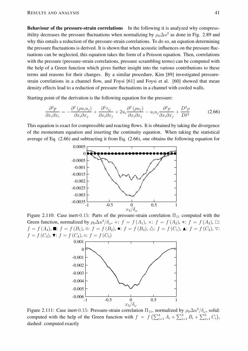
RESULTS AND ANALYSIS 41
Behaviour of the pressure-strain correlations In the following it is analyzed why compress-ibility decreases the pressure fluctuations when normalizing by ρ0∆u2 as done in Fig. 2.89 andwhy this entails a reduction of the pressure-strain correlations. To do so, an equation determiningthe pressure fluctuations is derived. It is shown that when acoustic influences on the pressure fluc-tuations can be neglected, this equation takes the form of a Poisson equation. Then, correlationswith the pressure (pressure-strain correlations, pressure scrambling terms) can be computed withthe help of a Green function which gives further insight into the various contributions to theseterms and reasons for their changes. By a similar procedure, Kim [89] investigated pressure-strain correlations in a channel flow, and Foysi [61] and Foysi et al. [60] showed that meandensity effects lead to a reduction of pressure fluctuations in a channel with cooled walls.
Starting point of the derivation is the following equation for the pressure:
∂2p
∂xi∂xi= −∂
2 (ρuiuj)
∂xi∂xj+
∂2τij∂xi∂xj
+ 2ui∂2 (ρuj)
∂xi∂xj− uiuj
∂2ρ
∂xi∂xj+D2ρ
Dt2(2.66)
This equation is exact for compressible and reacting flows. It is obtained by taking the divergenceof the momentum equation and inserting the continuity equation. When taking the statisticalaverage of Eq. (2.66) and subtracting it from Eq. (2.66), one obtains the following equation for
x3/δω10.50-0.5-1
0.0005
0
-0.0005
-0.001
-0.0015
-0.002
-0.0025
-0.003
-0.0035
Figure 2.110: Case inert-0.15: Parts of the pressure-strain correlation Π11 computed with theGreen function, normalized by ρ0∆u3/δω, +: f = f (A1), ×: f = f (A2), ∗: f = f (A3), �:f = f (A4), �: f = f (B1), ◦: f = f (B2), •: f = f (B3), 4: f = f (C1), N: f = f (C2), O:f = f (C3), H: f = f (C4), �: f = f (C5)
x3/δω10.50-0.5-1
0.001
0
-0.001
-0.002
-0.003
-0.004
-0.005
-0.006
Figure 2.111: Case inert-0.15: Pressure-strain correlation Π11, normalized by ρ0∆u3/δω, solid:computed with the help of the Green function with f = f
(∑4i=1 Ai +
∑3i=1 Bi +
∑5i=1 Ci
),
dashed: computed exactly

42 2. DNS OF INERT COMPRESSIBLE TURBULENT SHEAR LAYERS
the pressure fluctuations:
∂2p′
∂x2j
=− 2∂〈ui〉f∂xj
∂
∂xi
(〈ρ〉u′′j
)− 2
∂〈ui〉f∂xi
∂
∂xj
(〈ρ〉u′′j
)− ∂2
∂xi∂xj
(〈ρ〉u′′i u′′j − 〈ρu′′i u′′j 〉
)
− 2〈ρ〉u′′j∂2ui∂xi∂xj
− ρ′(∂〈ui〉f∂xi
)2
− ρ′∂〈ui〉f∂xj
∂〈uj〉f∂xi
− 2∂〈ui〉f∂xj
∂
∂xi
(ρ′u′′j
)− 2
∂〈ui〉f∂xi
∂
∂xj
(ρ′u′′j
)− 2
∂2〈ui〉f∂xi∂xj
(ρ′u′′j
)
− ∂2
∂xi∂xj
(ρ′u′′i u
′′j
)+D
2ρ′
Dt2+
∂2τ ′ij∂xi∂xj
(2.67)
For a fully developed turbulent flow that is periodic in x1- and x2-directions this equation simpli-fies to
∂2p′
∂x2j
=−〈ρ〉 ∂2
∂xixj
(u′′i u
′′j − 〈u′′i u′′j 〉
)
︸ ︷︷ ︸A1
−2〈ρ〉∂〈u1〉f∂x3
∂u′′3∂x1︸ ︷︷ ︸
A2
−2〈ρ〉∂〈u3〉f∂x3
(∂u′′1∂x1
+∂u′′2∂x2
+ 2∂u′′3∂x3
)
︸ ︷︷ ︸A3
−2〈ρ〉∂2〈u3〉f∂x2
3
u′′3︸ ︷︷ ︸
A4
−2∂〈ρ〉∂x3
∂
∂xj
(u′′3u
′′j − 〈u′′3u′′j 〉
)
︸ ︷︷ ︸B1
−∂2〈ρ〉∂x2
3
(u′′23 − 〈u′′23 〉
)
︸ ︷︷ ︸B2
−4u′′3∂〈ρ〉∂x3
∂〈u3〉f∂x3︸ ︷︷ ︸
B3
−2∂〈u1〉f∂x3
∂
∂x1
(ρ′u′′3)︸ ︷︷ ︸
C1
− ∂2
∂xi∂xj
(ρ′u′′i u
′′j − 〈ρ′u′′i u′′j 〉
)
︸ ︷︷ ︸C2
−2∂〈u3〉f∂x3
(∂
∂x1(ρ′u′′1) +
∂
∂x2(ρ′u′′2) + 2
∂
∂x3(ρ′u′′3)
)
︸ ︷︷ ︸C3
−2ρ′(∂〈u3〉f∂x3
)2
︸ ︷︷ ︸C4
−2ρ′u′′3∂2〈u3〉f∂x2
3︸ ︷︷ ︸C5
+D
2ρ′
Dt2︸ ︷︷ ︸C6
+∂2τ ′ij∂xi∂xj︸ ︷︷ ︸D
.
(2.68)
The operator D2/Dt2 is defined as
D2
Dt2:=
∂2
∂t2+ 2〈uj〉f
∂2
∂t∂xj+ 〈ui〉f〈uj〉f
∂2
∂xi∂xj. (2.69)
The terms on the RHS of Eq. (2.68) can be classified into terms that depend explicitly on themean density (A1 to A4), terms that depend on gradients of the mean density (B1 to B3), termsthat are caused by temporal and spatial variations of the density fluctuations with or without directcoupling to the velocity fluctuations (C1 to C6) and a term that is caused by viscous effects (D).The latter one is very small for the flows considered in this work and is neglected in the following.The termsA1 toA4 are the only ones that are present in an incompressible case (constant density).If considering the complete termC6 and assuming the isentropic relation p′ = 〈c〉2ρ′, a convectivewave equation for the pressure fluctuations is obtained [123]. For the inert shear layers studied

RESULTS AND ANALYSIS 43
here, term C6 turns out to be small according to DNS data. This makes Eq. (2.68) a Poissonequation for the pressure fluctuations.
The Poisson equation for p′ can be studied with the help of a Green function in order to ob-tain information about the contribution of the individual terms on the RHS. Applying a Fouriertransformation in the homogeneous directions, p (x1, x2, x3) → p (k1, k2, x3), and a coordinatetransformation in the transverse direction, x′3 = 2x3/L3, Eq. (2.68) becomes
(d2
dx′23− k2
1 − k22
)p (k1, k2, x
′3) = f (k1, k2, x
′3) (2.70)
with f denoting the terms on the RHS of Eq. (2.68). It is assumed that the gradients of thepressure fluctuations at the boundary of the computational domain, which is sufficiently far awayfrom the mixing layer, are small. Therefore,
∂p
∂x′3
∣∣∣∣x′3=±1
= 0. (2.71)
The Green function corresponding to Eqs. (2.70) and (2.71) is [89]:
G (k, x′3, x′′3) = −cosh [k (x′′3 − 1)] cosh [k (x′3 + 1)]
2k cosh (k) sinh (k), for x′3 < x′′3
G (k, x′3, x′′3) = −cosh [k (x′′3 + 1)] cosh [k (x′3 − 1)]
2k cosh (k) sinh (k), for x′3 > x′′3
(2.72)
x3/δω10.50-0.5-1
0.0002
0
-0.0002
-0.0004
-0.0006
-0.0008
-0.001
-0.0012
-0.0014
Figure 2.112: Case inert-0.7: Parts of the pressure-strain correlation Π11 computed with the Greenfunction, normalized by ρ0∆u3/δω, symbols as in Fig. 2.110
x3/δω10.50-0.5-1
0.00020
-0.0002-0.0004-0.0006-0.0008-0.001
-0.0012-0.0014-0.0016-0.0018-0.002
Figure 2.113: Case inert-0.7: Pressure-strain correlation Π11, normalized by ρ0∆u3/δω, solid:computed with the help of the Green function with f = f
(∑4i=1 Ai +
∑3i=1 Bi +
∑5i=1 Ci
),
lines as in Fig. 2.111

44 2. DNS OF INERT COMPRESSIBLE TURBULENT SHEAR LAYERS
x3/δω10.50-0.5-1
0.00010
-1e-04-0.0002-0.0003-0.0004-0.0005-0.0006-0.0007-0.0008
Figure 2.114: Case inert-1.1: Parts of the pressure-strain correlation Π11 computed with the Greenfunction, normalized by ρ0∆u3/δω, symbols as in Fig. 2.110
x3/δω10.50-0.5-1
0.0002
0
-0.0002
-0.0004
-0.0006
-0.0008
-0.001
-0.0012
-0.0014
Figure 2.115: Case inert-1.1: Pressure-strain correlation Π11, normalized by ρ0∆u3/δω, solid:computed with the help of the Green function with f = f
(∑4i=1 Ai +
∑3i=1 Bi +
∑5i=1 Ci
),
lines as in Fig. 2.111
for k 6= 0, where k = (k21 + k2
2)1/2 and
G (0, x′3, x′′3) = 0.5 (x′′3 − x′3) , for x′3 < x′′3
G (0, x′3, x′′3) = 0.5 (x′3 − x′′3) , for x′3 > x′′3
(2.73)
for k = 0. Consequently, the solution of Eq. (2.70) writes
p′ (x1, x2, x′3) =
∫ 1
−1
G ∗ f (x1, x2, x′′3) dx′′3 (2.74)
x3/δω10.50-0.5-1
0.0005
0
-0.0005
-0.001
-0.0015
-0.002
-0.0025
-0.003
-0.0035
Figure 2.116: Case inert-0.15: Parts of the pressure-strain correlation Π11 computed with theGreen function and with constant density ρ0, normalized by ρ0∆u3/δω, symbols as in Fig. 2.110

RESULTS AND ANALYSIS 45
x3/δω10.50-0.5-1
0.0002
0
-0.0002
-0.0004
-0.0006
-0.0008
-0.001
-0.0012
-0.0014
Figure 2.117: Case inert-0.7: Parts of the pressure-strain correlation Π11 computed with the Greenfunction and with constant density ρ0, normalized by ρ0∆u3/δω, symbols as in Fig. 2.110
x3/δω10.50-0.5-1
0.00010
-1e-04-0.0002-0.0003-0.0004-0.0005-0.0006-0.0007-0.0008-0.0009
Figure 2.118: Case inert-1.1: Parts of the pressure-strain correlation Π11 computed with the Greenfunction and with constant density ρ0, normalized by ρ0∆u3/δω, symbols as in Fig. 2.110
where the convolution G ∗ f represents the inverse Fourier transform of Gf ,
G∗f ′ (x1, x2, x′′3) =
1
(2π)2
∫ ∞
−∞dk1
∫ ∞
−∞dk2 exp (ikixi) G (k1, k2, x
′3, x′′3) f (k1, k2, x
′′3) . (2.75)
Multiplication with s′′ij and averaging, results in the pressure-strain correlations
Πij (x′3) =
∫ 1
−1
〈G ∗ f (x1, x2, x′′3) s′′ij (x1, x2, x
′3)〉dx′′3 (2.76)
Similarly, the pressure-scrambling terms are obtained when multiplying with ∂Y ′′/∂xi instead ofs′′ij . These terms are further studied in Sect. 2.4.4.2.
When inserting not the complete RHS f into Eq. (2.76), but only a part of it, e.g. term A1, it ispossible to see which of the terms on the RHS contributes most to the pressure fluctuations and towhat mechanisms the reduction of the pressure-strain correlations with compressibility are due.Figure 2.110 shows the contributions to the pressure-strain term, Π11 of case inert-0.15, computedthis way and averaged over the self-similar state. It can be seen that only terms A1 and A2 aresignificant, and all other terms can be neglected. When summing up all terms, the result, shownas a solid line in Fig. 2.111, corresponds well to Π11 computed directly as done in the previoussections. This justifies the neglection of terms D and C6 for this case. When increasing Mc, thecontribution from term C2, which is one of the terms involving density fluctuations starts to grow

46 2. DNS OF INERT COMPRESSIBLE TURBULENT SHEAR LAYERS
somewhat, however, it remains small compared to the contributions from terms A1 and A2 (cf.Figs. 2.112 and 2.114). Even though term C6, which is expected to represent acoustic effects,is neglected, the summation of the rest of the terms provides still a good approximation to Π11
as shown in Figs. 2.113 and 2.115. Since the analysis of the other pressure-strain terms givesqualitatively similar results, it can be concluded that acoustic effects do not play a significant rolefor the pressure-strain correlations of inert mixing layers in the convective Mach number rangeconsidered in this study.
A comparison between Figs. 2.110, 2.112 and 2.114 shows, that the contributions from terms A1
and A2 decrease with increasing Mc which corresponds to the same behaviour that has been no-ticed previously for the complete pressure-strain rates. To find out whether this is a consequenceof the mean density reduction (cf. Fig. 2.64) by compressibility, the mean density 〈ρ〉 appearingin terms A1 to A4 of Eq. (2.68) is set constant, i.e. ρ0 is inserted instead. The density fluctuationsin the other terms are set to zero. Figures 2.116 to 2.118 show the resulting contributions to Π11
when replacing the original terms on the RHS of Eq. (2.68) by these modified terms: The reduc-tion of the contributions from terms A1 and A2 with increasing Mc is still visible which excludesmean density effects to be the reason for this behaviour. Consequently, it must be caused bychanges in the velocity field.
Turbulent and gradient Mach numbers The turbulent Mach number
Mt =
√2k
〈c〉 (2.77)
is an indicator of the level of compressibility of the turbulence and can also be interpreted as theratio of the eddy-acoustic time scale τa to the turbulence time scale τt [63]. Fig. 2.119 showsthe increase of the turbulent Mach number with increasing Mc. However, Sarkar [161] showedfor homogeneously sheared turbulence that it is not the turbulent Mach number but the gradientMach number
Mg =Sl
〈c〉 , (2.78)
which steers the reduction of the TKE growth rate by a reduced level of turbulent production. InEq. (2.78), S denotes the mean shear and l a length scale in the direction of the mean shear. Sarkar[161] pointed out that an increase in turbulent Mach number reduced also the growth rate of theTKE, however considerably less than an increase inMg. The reason for the decrease withMt was
x3/δω
Mt
10.50-0.5-1
0.35
0.3
0.25
0.2
0.15
0.1
0.05
0
Figure 2.119: Turbulent Mach number Mt, symbols as in Fig. 2.63

RESULTS AND ANALYSIS 47
x3/δω
Mg
10.50-0.5-1
1.81.61.41.2
10.80.60.40.2
0
Figure 2.120: Gradient Mach number Mg, symbols as in Fig. 2.63
identified to be due to a contribution from pressure dilatation and dilatational dissipation. Thesefindings can also explain why compressibility effects are strong in shear layers and rather lackin boundary layers: The gradient Mach number in the latter ones is much smaller than in shearlayers. Pantano & Sarkar [123] pursued the investigations for the compressible mixing layer andalso found the gradient Mach number to be the key quantity that determines the reduction of thepressure-strain term. Figure 2.120 shows the gradient Mach number, computed with l = δω forthe inert mixing layers. In agreement with the just mentioned studies, it increases with increasingMc. Since both, Mt and Mg are affected by compressibility it is interesting to see whether bothquantities are correlated. Blaisdell et al. indeed found a correlation [12] which can be confirmedby the present results (Fig. 2.121). However, due to different initial conditions and the use ofanother length scale in the computation of Mg, the slopes of the approximately linear relations donot coincide.
Since the gradient Mach number can also be interpreted as the acoustic time scale τa dividedby the mean distortion time scale of the flow, τd, the ratio of the gradient Mach number to theturbulent Mach number,
Mg
Mt=τa/τdτa/τt
=τtτd, (2.79)
is the turbulence time scale, τt, divided by the mean distortion time scale and quantifies thedegree to which rapid-distortion effects govern the flow [63]. The approximately linear relationbetween Mg and Mt for the inert mixing layers makes this ratio constant at all convective Machnumbers that have been investigated and leads to the conclusion that such effects do not increase
Mg
Mt
1.81.61.41.210.80.60.40.20
0.550.5
0.450.4
0.350.3
0.250.2
0.150.1
0.050
Figure 2.121: Turbulent Mach number Mt plotted as a function of the gradient Mach numberMg.Symbols as in Fig. 2.63, solid line: Mt = 0.286Mg, dashed line: Mt = 0.159Mg

48 2. DNS OF INERT COMPRESSIBLE TURBULENT SHEAR LAYERS
significantly with Mc. This is in agreement with the findings of Freund et al. for the annular inertmixing layer [63].
Spectra Figure 2.122 shows the one-dimensional, streamwise spectra of the velocity u1 (u1′u1′∗
with u1′ denoting the velocity component u1 Fourier transformed in x1 direction and u1
′∗ itscomplex conjugate) after averaging over directions x2 and x3. None of the spectra shows signsof under-resolution like accumulation of energy at the highest wavenumbers. Mostly the higherwave numbers are affected by increasing compressibility and a decrease of the energy that iscontained in the highest wavenumbers (smallest scales) can be noticed. This is in agreement withthe structural changes that were noticed earlier, like the larger-scale ondulations that show themixing layers at higher convective Mach number in comparison to the simulation inert-0.15 (cf.Sect. 2.4.1). The spectra of the other velocity components evaluated in the streamwise and also inthe other homogeneous direction, which is the spanwise one, demonstrate a similar behaviour (notshown). Therefore, it can also be found in the spectra of the TKE in Fig. 2.123. A comparisonto the reference line with a slope of −5/3, which gives the energy fall-off in the inertial rangefor high Reynolds number turbulence [153], shows that the energy cascade follows this slope forat least a small part of the spectrum. However, due to the relatively small Reynolds number, alarge inertial range cannot be expected. Pantano & Sarkar [123] also present energy spectra thatshow a decrease in the highest wavenumbers with increasing Mc, but they do not comment on
k1δω,0
Eu
1001010.1
1
1e-05
1e-10
1e-15
1e-20
Figure 2.122: One-dimensional, streamwise spectrum of u1/∆u at the beginning of the self-similar state, solid: inert-0.15, dashed: inert-0.7, dotted: inert-1.1
k1δω,0
Ek
1001010.10.01
0.01
0.0001
1e-06
1e-08
1e-10
1e-12
1e-14
Figure 2.123: One-dimensional, streamwise spectrum of TKE k/∆u2 at the beginning of theself-similar state, solid: inert-0.15, dashed: inert-0.7, dotted: inert-1.1, the straight line has −5/3
slope

RESULTS AND ANALYSIS 49
k1δω,0
Eu·k
2 1/δ
2 ω,0
1001010.1
0.0001
1e-06
1e-08
1e-10
1e-12
1e-14
1e-16
1e-18
1e-20
Figure 2.124: One-dimensional, streamwise dissipation spectrum (spectrum of u1/∆u multipliedwith (k1δω,0)2) at the beginning of the self-similar state, solid: inert-0.15, dashed: inert-0.7,dotted: inert-1.1this feature.
One-dimensional dissipation spectra, evaluated as k21u′u′∗, are shown in Fig. 2.124. Compared
to the TKE spectra there is more ’dissipated energy’ situated in the higher wave numbers whichis to be expected since the dissipation of energy takes mostly place in the smallest scales. Again,increasing compressibility leads to a reduction of the energy content in the highest wavenumbers.
2.4.4.2 Scalar mixing
In the present test cases, the species mass fractions are active, but non-reactive scalars. They arecalled ’active’ as they influence the flow field by their molecular weight through the density andby the transport coefficients that depend among other thermodynamic variables (the temperatureand partially the pressure) on their concentration.
The influence of compressibility on molecular mixing has been investigated previously mostlyby experimentalists. While some authors report a small increase of mixing efficiency with com-pressibility [27, 28, 45], others found no apparent dependency on the convective Mach number[78] or even encountered a decrease [70]. However, some of these experiments, e.g. [27] are notfully spatially resolved as pointed out by [114]. Freund et al. [64] found an increase in mixing ef-ficiency for their DNS of annular mixing layers between Mc = 0.1 and Mc = 1.54 but a decreasefor their highest Mach number case Mc = 1.8 which they are unable to explain. Many of thesestudies also deal with the entrainment ratio, which is the average amount of fluid entrained intothe mixing layer from the high-speed side divided by the average amount of fluid entrained fromthe low-speed side, and found it significantly altered by compresssibility. However, due to thesymmetry of the temporally evolving mixing layer, corresponding studies can not be performedfor the present configuration.
Mean profile and variance The differences between the Favre averaged profiles of the oxygenmass fraction at different Mc (Fig. 2.125) are larger than those of the streamwise velocity profiles(Fig. 2.66). The case inert-0.15 seems to have a flatter and more extended linear region in thecenter of the shear layer than the shear layers at higher Mc the profiles of which are fuller andcloser to the shape of a hyperbolic-tangent or an error function.
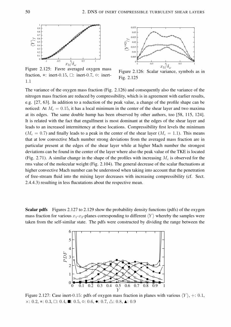
50 2. DNS OF INERT COMPRESSIBLE TURBULENT SHEAR LAYERS
x3/δω
〈Y〉 f
10.50-0.5-1
10.90.80.70.60.50.40.30.20.1
0
Figure 2.125: Favre averaged oxygen massfraction, ∗: inert-0.15, �: inert-0.7, ◦: inert-1.1
x3/δω
〈Y′′2〉 f
10.50-0.5-1
0.035
0.03
0.025
0.02
0.015
0.01
0.005
0
Figure 2.126: Scalar variance, symbols as inFig. 2.125
The variance of the oxygen mass fraction (Fig. 2.126) and consequently also the variance of thenitrogen mass fraction are reduced by compressibility, which is in agreement with earlier results,e.g. [27, 63]. In addition to a reduction of the peak value, a change of the profile shape can benoticed: At Mc = 0.15, it has a local minimum in the center of the shear layer and two maximaat its edges. The same double hump has been observed by other authors, too [58, 115, 124].It is related with the fact that engulfment is most dominant at the edges of the shear layer andleads to an increased intermittency at these locations. Compressibility first levels the minimum(Mc = 0.7) and finally leads to a peak in the center of the shear layer (Mc = 1.1). This meansthat at low convective Mach number strong deviations from the averaged mass fraction are inparticular present at the edges of the shear layer while at higher Mach number the strongestdeviations can be found in the center of the layer where also the peak value of the TKE is located(Fig. 2.71). A similar change in the shape of the profiles with increasing Mc is observed for therms value of the molecular weight (Fig. 2.104). The general decrease of the scalar fluctuations athigher convective Mach number can be understood when taking into account that the penetrationof free-stream fluid into the mixing layer decreases with increasing compressibility (cf. Sect.2.4.4.3) resulting in less flucutations about the respective mean.
Scalar pdfs Figures 2.127 to 2.129 show the probability density functions (pdfs) of the oxygenmass fraction for various x1-x2-planes corresponding to different 〈Y 〉 whereby the samples weretaken from the self-similar state. The pdfs were constructed by dividing the range between the
Y
10.90.80.70.60.50.40.30.20.10
6
5
4
3
2
1
0
Figure 2.127: Case inert-0.15: pdfs of oxygen mass fraction in planes with various 〈Y 〉, +: 0.1,×: 0.2, ∗: 0.3, �: 0.4, �: 0.5, ◦: 0.6, •: 0.7,4: 0.8, N: 0.9

RESULTS AND ANALYSIS 51
Y
10.90.80.70.60.50.40.30.20.10
6
5
4
3
2
1
0
Figure 2.128: Case inert-0.7: pdfs of oxygen mass fraction in planes with various 〈Y 〉, +: 0.1,×: 0.2, ∗: 0.3, �: 0.4, �: 0.5, ◦: 0.6, •: 0.7,4: 0.8, N: 0.9
Y
10.90.80.70.60.50.40.30.20.10
6
5
4
3
2
1
0
Figure 2.129: Case inert-1.1: pdfs of oxygen mass fraction in planes with various 〈Y 〉, +: 0.1,×: 0.2, ∗: 0.3, �: 0.4, �: 0.5, ◦: 0.6, •: 0.7,4: 0.8, N: 0.9
x3/δω
10.90.80.70.60.50.40.30.20.10
4
3.5
3
2.5
2
1.5
1
0.5
0
Figure 2.130: Pdfs of oxygen mass fraction in the plane with 〈Y 〉 = 0.3 (solid) and 〈Y 〉 = 0.5
(dashed), symbols as in Fig. 2.125
maximum value (1.) and the minimum value (0.) in 50 bins and normalizing such that:∫ 1
0
PDF (Y ) = 1. (2.80)
Comparing the pdfs for the different convective Mach numbers, one can see that for Mc = 0.15
more pure, unmixed fluid is present at 〈Y 〉 = 0.8, 0.7, 0.3 and 0.2 than for the other cases. Thisis in agreement with the stronger engulfment of this shear layer (cf. Sect. 2.4.4.3). Comparingdirectly the pdfs for certain 〈Y 〉, as it is done in Figs. 2.130, it is visible that the higher the

52 2. DNS OF INERT COMPRESSIBLE TURBULENT SHEAR LAYERS
Mach number the narrower and more pointed the pdfs. This is directly related with the lowerfluctuations noticed at higher Mach number.
Figures 2.127 to 2.129 also show that the most probable value of the mass fraction, i.e. the max-imum of the pdfs, varies across the layer. At each side of the layer, it is closer to the free-streamvalue of that side which proofs that the fluid gets mixed into the layer at the edges. Such pdfs arecalled marching pdfs. The other cathegory that pdfs can fall in are the so-called non-marchingpdfs in which the most probable value is independent of the position in the layer. Rogers &Moser [152] found marching and non-marching pdfs in their incompressible mixing layer de-pending upon the initial conditions. The layer with the largest initial forcing, which developedlarge roller structures and braid regions, had a non-marching scalar pdf which the authors sug-gested to be caused by pure fluid which is engulfed by the large structures. As all the pdfs foundhere are marching, it is expected to find the engulfed fluid volume rather small compared to themixed one, which is confirmed and further investigated in Sect. 2.4.4.3. Clemens & Mungal[27] also found marching pdfs at both, low and high convective Mach number with the pdfs atlow convective Mach number being broader. They elucidated what types of turbulent structuresare responsible for the nature of the pdfs: Narrow, marching pdfs are caused by mixing layersthe structures of which closely resemble the mean profiles being uniform in the streamwise andsloped in the transverse direction. Broad and non-marching pdfs are the consequence of structuresthat are sloped in the streamwise direction and uniform in the transverse direction. As the pdfsthat are encountered here and also by these authors are relatively broad and marching both kind ofturbulent structures must be present in the mixing layer. However, with the high compressibilitypdfs being narrower, the structures of this mixing layer resemble more closely the mean profilewhich is equivalent to having less fluctuations.
Mixing efficiency The mixing efficiency measures the mixing of the fluid in the layer that takesplace at the molecular level. Following Freund et al. [64], it is defined in terms of the scalar pdfP (Y, x3) measured at different transverse positions:
δMδY
=1
δY
∫ ∞
−∞dx3
∫ 1−ε
ε
dY P (Y, x3) (2.81)
where δY denotes the 99% scalar thickness. The choice of the small parameter ε influences theresulting mixing efficiency. The higher ε is chosen, the more fluid is considered unmixed. Figure2.131 shows the mixing efficiency for different ε. Since 50 bins have been used to determine the
Mc
δ M/δY
1.21.110.90.80.70.60.50.40.30.20.1
0.86
0.84
0.82
0.8
0.78
0.76
0.74
0.72
Figure 2.131: Mixing efficiency, �: ε = 0.02, ∗: ε = 0.04

RESULTS AND ANALYSIS 53
pdfs, ε = 0.02 corresponds to defining the fluid in the extreme bins to be pure and ε = 0.04,to defining the fluid in the two outer bins to be pure. In the figure it can be seen that there isan increasing trend in the mixing efficiency from low to high convective Mach number whichis in agreement with the results of Freund et al. [64]. In other words, with increasing Mc,there is less free-stream fluid present, i.e. fluid with species mass fractions of 0 ≤ Yα < ε
or 1 − ε < Yα ≤ 1. This is consistent with the already observed decrease in mass fractionfluctuations and with reduced engulfment (cf. Sect. 2.4.4.3).
Scalar variance transport equation The transport equation of the scalar variance reads fortemporally evolving shear layers:
∂
∂t〈12ρY ′′α
2〉 =− 1
2〈u3〉f
∂
∂x3〈ρY ′′α 2〉 − 1
2
∂
∂x3〈ρu′′3Y ′′α 2〉
− 〈ρY ′′α u′′3〉∂〈Yα〉f∂x3
− 1
2〈ρY ′′α 2〉∂〈u3〉f
∂x3
− ∂
∂x3
〈ρYαY ′′α Vα3〉+ 〈ρYαVαi∂Y ′′α∂xi〉
(2.82)
The first term on the right hand side describes mean convection, the second is called turbulenttransport, the third and fourth turbulent production, the fifth molecular diffusion and the last one is
x3/δω10.50-0.5-1
0.0075
0.005
0.0025
0
-0.0025
-0.005
Figure 2.132: Major terms in the scalar variance transport equation, normalized by ρ0∆u/δω,solid: turbulent production, dashed: turbulent transport, dotted: dissipation rate, symbols as inFig. 2.125
x3/δω10.50-0.5-1
0.001
0
-0.001
-0.002
-0.003
-0.004
-0.005
Figure 2.133: Parts of the scalar dissipation rate, solid: 〈ρYαVαi ∂Yα∂xi〉, dashed: 〈ρYαVαi〉∂〈Yα〉f∂xi
,normalized by ρ0∆u/δω, symbols as in Fig. 2.125

54 2. DNS OF INERT COMPRESSIBLE TURBULENT SHEAR LAYERS
the dissipation term. Figure 2.132 shows the most important terms: Positive turbulent productionis the major source term, the negative dissipation rate is the major sink and the turbulent transportis negative in the center of the shear layer and positive at its edges at Mc = 0.15 and oscillatesaround zero for higher convective Mach numbers.
The most important change that occurs with increasing Mc is the reduction of the turbulent pro-duction. In addition, a decrease in the magnitude of the turbulent transport and of the dissipationrate is noticed. The dissipation rate can be split up into:
εY = 〈ρYαVαi∂Y ′′α∂xi〉 = 〈ρYαVαi
∂Yα∂xi〉 − 〈ρYαVαi〉
∂〈Yα〉f∂xi
(2.83)
Figure 2.133 shows that the second part on the RHS, which is the product of two mean values,can be neglected with respect to the first part, so that
εY ≈ 〈ρYαVαi∂Yα∂xi〉 (2.84)
is a valid approximation.
Scalar fluxes Figures 2.134 and 2.135 show the most important scalar fluxes, 〈ρu′′1Y ′′α 〉 and〈ρu′′3Y ′′α 〉. It can be seen that both, the streamwise scalar flux, 〈ρu′′1Y ′′α 〉, as well as the transversescalar flux, 〈ρu′′3Y ′′α 〉, reduce with increasing compressibility. The reduction of the latter one, inparticular from Mc = 0.7 to Mc = 1.1, however, is considerably larger than the reduction of thestreamwise flux which has also been noticed by Freund et al. [64]. The spanwise scalar flux (notshown) is one order of magnitude smaller than the other scalar fluxes and not investigated further.
x3/δω
〈ρu′′ 1Y′′ 〉/
(ρ0∆u
)
10.50-0.5-1
0.014
0.012
0.01
0.008
0.006
0.004
0.002
0
-0.002
Figure 2.134: Scalar flux 〈ρu′′1Y ′′α 〉 of oxygen, normalized by ρ0∆u, symbols as in Fig. 2.125
x3/δω
〈ρu′′ 3Y′′ 〉/
(ρ0∆u
)
10.50-0.5-1
0
-0.002
-0.004
-0.006
-0.008
-0.01
-0.012
Figure 2.135: Scalar flux 〈ρu′′3Y ′′α 〉 of oxygen, normalized by ρ0∆u, symbols as in Fig. 2.125

RESULTS AND ANALYSIS 55
Transport equations of scalar fluxes The general form of the transport equation for the scalarfluxes in Cartesian coordinates is:
∂
∂t〈ρu′′i Y ′′α 〉 =− 〈uj〉f
∂
∂xj〈ρu′′i Y ′′α 〉 −
∂
∂xj〈ρu′′i u′′jY ′′α 〉
− 〈ρu′′i Y ′′α 〉∂〈uj〉f∂xj
− 〈ρu′′jY ′′α 〉∂〈ui〉f∂xj
− 〈ρu′′i u′′j 〉∂〈Yα〉f∂xj
+ 〈p∂Y′′α
∂xi〉
− ∂
∂xj〈pY ′′α 〉δij +
∂
∂xj〈τijY ′′α 〉 −
∂
∂xj〈u′′i ρYαVαj〉
− 〈τij∂Y ′′α∂xj〉+ 〈ρY Vαj
∂u′′i∂xj〉
(2.85)
The first term on the RHS denotes convection, the second term is the turbulent transport and thenext three terms are production terms. The term in the third line is the pressure scalar-gradientcorrelation and the terms in the fourth line are diffusion terms. The last two terms describe thedissipation.
For a shear layer which is periodic in x1- and x2-directions the transport equation in the x1-direction can be simplified to
∂
∂t〈ρu′′1Y ′′α 〉 =− 〈u3〉f
∂
∂x3〈ρu′′1Y ′′α 〉 −
∂
∂x3〈ρu′′1u′′3Y ′′α 〉
− 〈ρu′′1Y ′′α 〉∂〈u3〉f∂x3
− 〈ρu′′3Y ′′α 〉∂〈u1〉f∂x3
− 〈ρu′′1u′′3〉∂〈Yα〉f∂x3
+ 〈p∂Y′′α
∂x1
〉
+∂
∂x3
〈τ13Y′′α 〉 −
∂
∂x3
〈u′′1ρYαVα3〉
− 〈τ1j∂Y ′′α∂xj〉+ 〈ρYαVαj
∂u′′1∂xj〉.
(2.86)
The resulting equation for the flux in the x3-direction is:
∂
∂t〈ρu′′3Y ′′α 〉 =− 〈u3〉f
∂
∂x3〈ρu′′3Y ′′α 〉 −
∂
∂x3〈ρu′′3u′′3Y ′′α 〉
− 2〈ρu′′3Y ′′α 〉∂〈u3〉f∂x3
− 〈ρu′′3u′′3〉∂〈Yα〉f∂x3
+ 〈p∂Y′′α
∂x3
〉
− ∂
∂x3
〈pY ′′α 〉+∂
∂x3
〈τ33Y′′α 〉 −
∂
∂x3
〈u′′3ρYαVα3〉
− 〈τ3j∂Y ′′α∂xj〉+ 〈ρYαVαj
∂u′′3∂xj〉.
(2.87)

56 2. DNS OF INERT COMPRESSIBLE TURBULENT SHEAR LAYERS
The pressure scalar-gradient correlation can also be written as
〈p∂Y′′α
∂xi〉 = 〈p〉∂〈Yα〉
∂xi− 〈p〉∂〈Yα〉f
∂xi+ 〈p′∂Y
′′α
∂xi〉. (2.88)
For the x1-direction this becomes
〈p∂Y′′α
∂x1〉 = 〈p′∂Y
′′α
∂x1〉, (2.89)
and for the x3-direction:
〈p∂Y′′α
∂x3〉 = 〈p〉∂〈Yα〉
∂x3− 〈p〉∂〈Yα〉f
∂x3+ 〈p′∂Y
′′α
∂x3〉 (2.90)
is obtained.
In the following, the changes due to compressibility of the major terms in these equations areinvestigated. The major terms are the production, the diffusion, the dissipation rates and theturbulent transport as well as the correlation between the pressure fluctuations and the spatialderivatives of the mass fraction fluctuations (third term on the RHS of Eq. (2.88)).
Figures 2.136 and 2.137 show the two major production terms of the streamwise scalar flux whichare the ones involving the mean gradient of the streamwise velocity and the mean gradient of thescalar mass fraction (second and third term in the second line of Eq. (2.86)). For the transversescalar flux, only the latter one (second term in the second line of Eq. (2.87)), which is shown inFig. 2.138, is important. It is negative and constitutes a source term since the transverse flux itselfis also negative (Fig. 2.135). All production terms are reduced by compressibility. Particularlystriking is the reduction between Mc = 0.15 and Mc = 0.7. The further increase to Mc = 1.1
seems to have less effect which could indicate an asymptotic behaviour. The reduction of the
x3/δω
−〈ρu′′ 3Y′′ α〉∂〈u
1〉 f
∂x
3
δ ωρ
0∆u
2
10.50-0.5-1
0.009
0.008
0.007
0.006
0.005
0.004
0.003
0.002
0.001
0
Figure 2.136: Part of the streamwise scalarflux production, normalized by ρ0∆u2/δω,symbols as in Fig. 2.125
x3/δω
−〈ρu′′ 1u′′ 3〉∂〈Yα〉 f
∂x
3
δ ωρ
0∆u
2
10.50-0.5-1
0.006
0.005
0.004
0.003
0.002
0.001
0
-0.001
Figure 2.137: Part of the streamwise scalarflux production, normalized by ρ0∆u2/δω,symbols as in Fig. 2.125
x3/δω
−〈ρu′′ 3u′′ 3〉∂〈Yα〉 f
∂x
3
δ ωρ
0∆u
2
10.50-0.5-1
0-0.001-0.002-0.003-0.004-0.005-0.006-0.007-0.008-0.009-0.01
Figure 2.138: Part of the transverse scalar fluxproduction, normalized by ρ0∆u2/δω, symbolsas in Fig. 2.125
x3/δω
−∂∂x
3〈pY′′ α〉
δ ωρ
0∆u
2
10.50-0.5-1
0.010.0080.0060.0040.002
0-0.002-0.004-0.006-0.008
-0.01
Figure 2.139: Major part of the diffusionof the transverse scalar flux, normalized byρ0∆u2/δω, symbols as in Fig. 2.125

RESULTS AND ANALYSIS 57
x3/δω
−〈τ 1j∂Y′′ α
∂xj〉
δ ωρ
0∆u
2
10.50-0.5-1
5e-05
0
-5e-05
-0.0001
-0.00015
-0.0002
-0.00025
Figure 2.140: Part of the dissipation rateof the streamwise scalar flux, normalized byρ0∆u2/δω, symbols as in Fig. 2.125
x3/δω
−〈τ 3j∂Y′′ α
∂xj〉
δ ωρ
0∆u
2
10.50-0.5-1
0.0003
0.00025
0.0002
0.00015
0.0001
5e-05
0
Figure 2.141: Part of the dissipation rateof the transverse scalar flux, normalized byρ0∆u2/δω, symbols as in Fig. 2.125
x3/δω
〈ρYVαj∂u′′ 1
∂xj〉
δ ωρ
0∆u
2
10.50-0.5-1
0
-5e-05
-0.0001
-0.00015
-0.0002
-0.00025
-0.0003
Figure 2.142: Part of the dissipation rateof the streamwise scalar flux, normalized byρ0∆u2/δω, symbols as in Fig. 2.125
x3/δω〈ρYαVαj∂u′′ 3
∂xj〉
δ ωρ
0∆u
2
10.50-0.5-1
0.0004
0.00035
0.0003
0.00025
0.0002
0.00015
0.0001
5e-05
0
Figure 2.143: Part of the dissipation rateof the transverse scalar flux, normalized byρ0∆u2/δω, symbols as in Fig. 2.125
scalar flux production is closely related with the reduction of the Reynolds stresses, which appearas factors in the part involving the mean mass fraction gradients, and with the reduction of thescalar fluxes themselves which are factors in the parts with the mean velocity gradients.
From the diffusion terms, only the first term in the third line of Eq. (2.87) plays a major role. Itis shown in Fig. 2.139 and decreases with increasing compressibility.
The reduction of the two parts of the dissipation rate of each scalar flux, respectively, (Figs.2.140 to 2.143) is not as strong as the reduction of the production which is similar to what hasbeen noticed earlier for production and dissipation rate of the Reynolds stresses and the scalarvariance.
Figures 2.144 and 2.145 show the turbulent transport of the streamwise and transverse scalar flux.It can be seen that for Mc = 0.15, the direction of the turbulent transport for both fluxes is fromthe center to the edges of the mixing layer. The turbulent transport decreases with increasingcompressibility and is strongly damped for the higher convective Mach numbers.
x3/δω
−∂∂x
3〈ρu′′ 1u′′ 3Y′′ α〉
δ ωρ
0∆u
2
10.50-0.5-1
0.0020.0015
0.0010.0005
0-0.0005
-0.001-0.0015
-0.002-0.0025
-0.003
Figure 2.144: Turbulent transport of thestreamwise scalar flux, normalized byρ0∆u2/δω, symbols as in Fig. 2.125
x3/δω
−∂∂x
3〈ρu′′ 3u′′ 3Y′′ α〉
δ ωρ
0∆u
2
10.50-0.5-1
0.004
0.003
0.002
0.001
0
-0.001
-0.002
-0.003
Figure 2.145: Turbulent transport of the trans-verse scalar flux, normalized by ρ0∆u2/δω,symbols as in Fig. 2.125

58 2. DNS OF INERT COMPRESSIBLE TURBULENT SHEAR LAYERS
x3/δω
〈p′∂Y′′ α
∂x
1〉
δ ωρ
0∆u
2
10.50-0.5-1
0
-0.002
-0.004
-0.006
-0.008
-0.01
-0.012
Figure 2.146: Pressure-scrambling term instreamwise direction, ΠY 1, normalized byρ0∆u2/δω, symbols as in Fig. 2.125
x3/δω
〈p′∂Y′′ α
∂x
3〉
δ ωρ
0∆u
2
10.50-0.5-1
0.0140.012
0.010.0080.0060.0040.002
0-0.002-0.004-0.006
Figure 2.147: Pressure-scrambling term intransverse direction, ΠY 3, normalized byρ0∆u2/δω, symbols as in Fig. 2.125
The reduction of the correlation between the pressure fluctuations and the spatial derivatives ofthe mass fraction fluctuations (last term in Eq. (2.88)) with compressibility is more pronouncedfor the streamwise derivative than for the transverse derivative (Figs. 2.146 and 2.147). This term,ΠY i, is also called pressure-scrambling term [100]. While it is purely negative and therefore a sinkfor the streamwise scalar flux (Fig. 2.146), it changes sign for the transverse flux: It is positiveand therefore a sink for the negative transverse scalar flux in the center of the mixing layer anda source at the mixing layer edges (Fig. 2.147). The reduction of the pressure-scrambling termswith increasing Mc is further investigated in the next paragraph.
Behaviour of the pressure-scrambling terms In Section 2.4.4.1, the pressure-strain correla-tions were computed and analyzed with the help of a Green function for the Poisson equation ofthe pressure fluctuations, Eq. (2.68). A corresponding procedure permits a closer investigation ofthe pressure-scrambling terms, ΠY i = 〈p′ ∂Y ′′α
∂xi〉, and of the reason for their reduction with increas-
ing Mc. Similar to the pressure-strain correlations in Eq. (2.76), the pressure scrambling termscan be computed by
ΠY i (x′3) =
∫ 1
−1
〈G ∗ f (x1, x2, x′′3)∂Y ′′
∂xi(x1, x2, x
′3)〉dx′′3 (2.91)
with the Green function G (cf. Eqs. (2.72) and (2.72)) and the source term f which correspondsto the RHS of Eq. (2.68). When inserting the terms on the RHS of Eq. (2.68) separately, the
x3/δω10.50-0.5-1
0.004
0.003
0.002
0.001
0
-0.001
-0.002
-0.003
Figure 2.148: Case inert-0.15: Parts of thepressure-scrambling term ΠY 3 computed withthe Green function, normalized by ρ0∆u/δω,+: f = f (A1), ×: f = f (A2), ∗: f =
f (A3), �: f = f (A4), �: f = f (B1), ◦: f =
f (B2), •: f = f (B3), 4: f = f (C1), N:f = f (C2), O: f = f (C3), H: f = f (C4), ♦:f = f (C5)
x3/δω10.50-0.5-1
0.0140.012
0.010.0080.0060.0040.002
0-0.002-0.004-0.006
Figure 2.149: Case inert-0.15: Pressure-scrambling term ΠY 3, normalizedby ρ0∆u/δω, solid: computed withthe help of the Green function withf = f
(∑4i=1 Ai +
∑3i=1 Bi +
∑5i=1 Ci
),
dashed: computed exactly

RESULTS AND ANALYSIS 59
x3/δω10.50-0.5-1
0.00450.004
0.00350.003
0.00250.002
0.00150.001
0.00050
-0.0005-0.001
Figure 2.150: Case inert-0.7: Parts of thepressure-scrambling term ΠY 3 computed withthe Green function, normalized by ρ0∆u/δω,symbols as in Fig. 2.148
x3/δω10.50-0.5-1
0.007
0.006
0.005
0.004
0.003
0.002
0.001
0
-0.001
-0.002
Figure 2.151: Case inert-0.7: Pressure-scrambling term ΠY 3, normalizedby ρ0∆u/δω, solid: computed withthe help of the Green function withf = f
(∑4i=1 Ai +
∑3i=1 Bi +
∑5i=1 Ci
),
lines as in Fig. 2.149
x3/δω10.50-0.5-1
0.0035
0.003
0.0025
0.002
0.0015
0.001
0.0005
0
-0.0005
Figure 2.152: Case inert-1.1: Parts of thepressure-scrambling term ΠY 3 computed withthe Green function, normalized by ρ0∆u/δω,symbols as in Fig. 2.148
x3/δω10.50-0.5-1
0.0040.0035
0.0030.0025
0.0020.0015
0.0010.0005
0-0.0005
-0.001
Figure 2.153: Case inert-1.1: Pressure-scrambling term ΠY 3, normalizedby ρ0∆u/δω, solid: computed withthe help of the Green function withf = f
(∑4i=1 Ai +
∑3i=1 Bi +
∑5i=1 Ci
),
lines as in Fig. 2.149
split-up of ΠY 3 in Fig. 2.148 is obtained for case inert-0.15. Since the results for the otherpressure-scrambling terms are qualitatively the same, just ΠY 3 is analyzed in the following. Asfor the pressure-strain correlations, only terms A1 and A2 contribute significantly to the completecorrelation. The comparison of ΠY 3 computed without terms C6 and D with the exact term inFig. 2.149, shows that the neglection of C6 and D is justified. The same conclusions apply to thepressure-scrambling terms at higher convective Mach numbers (Figs. 2.150 to 2.153).
To obtain Figs. 2.154 to 2.156 modified source terms with constant density, equal to ρ0 were
x3/δω10.50-0.5-1
0.004
0.003
0.002
0.001
0
-0.001
-0.002
-0.003
Figure 2.154: Case inert-0.15: Parts of thepressure-scrambling term ΠY 3 computed withthe Green function and with constant densityρ0, normalized by ρ0∆u/δω, symbols as in Fig.2.148
x3/δω10.50-0.5-1
0.00450.004
0.00350.003
0.00250.002
0.00150.001
0.00050
-0.0005-0.001
Figure 2.155: Case inert-0.7: Parts of thepressure-scrambling term ΠY 3 computed withthe Green function and with constant densityρ0, normalized by ρ0∆u/δω, symbols as in Fig.2.148
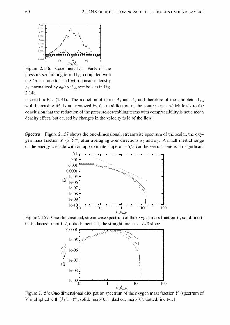
60 2. DNS OF INERT COMPRESSIBLE TURBULENT SHEAR LAYERS
x3/δω10.50-0.5-1
0.004
0.0035
0.003
0.0025
0.002
0.0015
0.001
0.0005
0
-0.0005
Figure 2.156: Case inert-1.1: Parts of thepressure-scrambling term ΠY 3 computed withthe Green function and with constant densityρ0, normalized by ρ0∆u/δω, symbols as in Fig.2.148inserted in Eq. (2.91). The reduction of terms A1 and A2 and therefore of the complete ΠY 3
with increasing Mc is not removed by the modification of the source terms which leads to theconclusion that the reduction of the pressure-scrambling terms with compressibility is not a meandensity effect, but caused by changes in the velocity field of the flow.
Spectra Figure 2.157 shows the one-dimensional, streamwise spectrum of the scalar, the oxy-gen mass fraction Y (Y ′Y ′∗) after averaging over directions x2 and x3. A small inertial rangeof the energy cascade with an approximate slope of −5/3 can be seen. There is no significant
k1δω,0
EY
1001010.10.01
0.10.01
0.0010.00011e-051e-061e-071e-081e-091e-10
Figure 2.157: One-dimensional, streamwise spectrum of the oxygen mass fraction Y , solid: inert-0.15, dashed: inert-0.7, dotted: inert-1.1, the straight line has −5/3 slope
k1δω,0
EY·k
2 1/δ
2 ω,0
1001010.1
0.0001
1e-05
1e-06
1e-07
1e-08
1e-09
Figure 2.158: One-dimensional dissipation spectrum of the oxygen mass fraction Y (spectrum ofY multiplied with (k1δω,0)2), solid: inert-0.15, dashed: inert-0.7, dotted: inert-1.1

RESULTS AND ANALYSIS 61
accumulation of energy in the highest wavenumbers which would be a sign of under-resolution.The behaviour with increasing compressibility corresponds to the one noticed for the spectra ofother quantities (cf. Sect. 2.4.4.1), like the TKE: The energy content in the highest wavenumbersdecreases when the convective Mach number rises. The scalar dissipation spectrum in Fig. 2.158,evaluated as k2
1Y′Y ′∗, peaks at a higher wavenumber than the scalar energy spectrum and shows
a similar behaviour for the highest wavenumbers with increasing compressibility.
2.4.4.3 Entrainment
In this section, the processes by which surrounding fluid enters the mixing layer and becomes apart of it is investigated. The focus is on the effects that compressibility has on this entrainmentmechanism.
While entrainment has often been described as an engulfment of large packets of irrotationalfluid from the surrounding non-turbulent region by the action of large-scale coherent structuresfollowed by disintegration and acquisition of vorticity well within the turbulent region, a recentstudy by Mathew & Basu [105] showed that a circular mixing layer grows by nibbling, a fast,small-scale process occurring very close to the turbulent-nonturbulent interface. The engulfedfluid volume, on the contrary, was revealed to be very small compared to the total volume ofthe turbulent region. These results have been confirmed by subsequent PIV measurements in alaboratory jet [186].
In this section, studies similar to those found in [105] for a cylindrical, incompressible mixinglayer are performed with the DNS data of the inert, plane mixing layers at different convectiveMach number.
Measurement of volumes To numerically measure the engulfed fluid, one has to define firsta criterion to distinguish between ambient fluid regions and the mixing layer which contains theengulfed fluid. Engulfed fluid lies inside the turbulent region but still has the scalar concentrationand the low vorticity levels of the freestream fluid. Here, fixed thresholds are used to distinguishbetween ambient fluid, engulfed fluid and the rest of the mixing layer, which consists of mixedfluid. One threshold concerns the magnitude of the vorticity and one the scalar value. For the
Figure 2.159: Case inert-0.15: Instanta-neous vorticity field, normalized by 〈ω〉max,x1-x3-plane in the middle of the computa-tional domain at τω = 286, isoline at 0.1 isshown
Figure 2.160: Case inert-0.15: Instanta-neous mass fraction field ofO2, x1-x3-planein the middle of the computational domainat τω = 286, isolines YO2 = 0.05 and 0.95
are shown
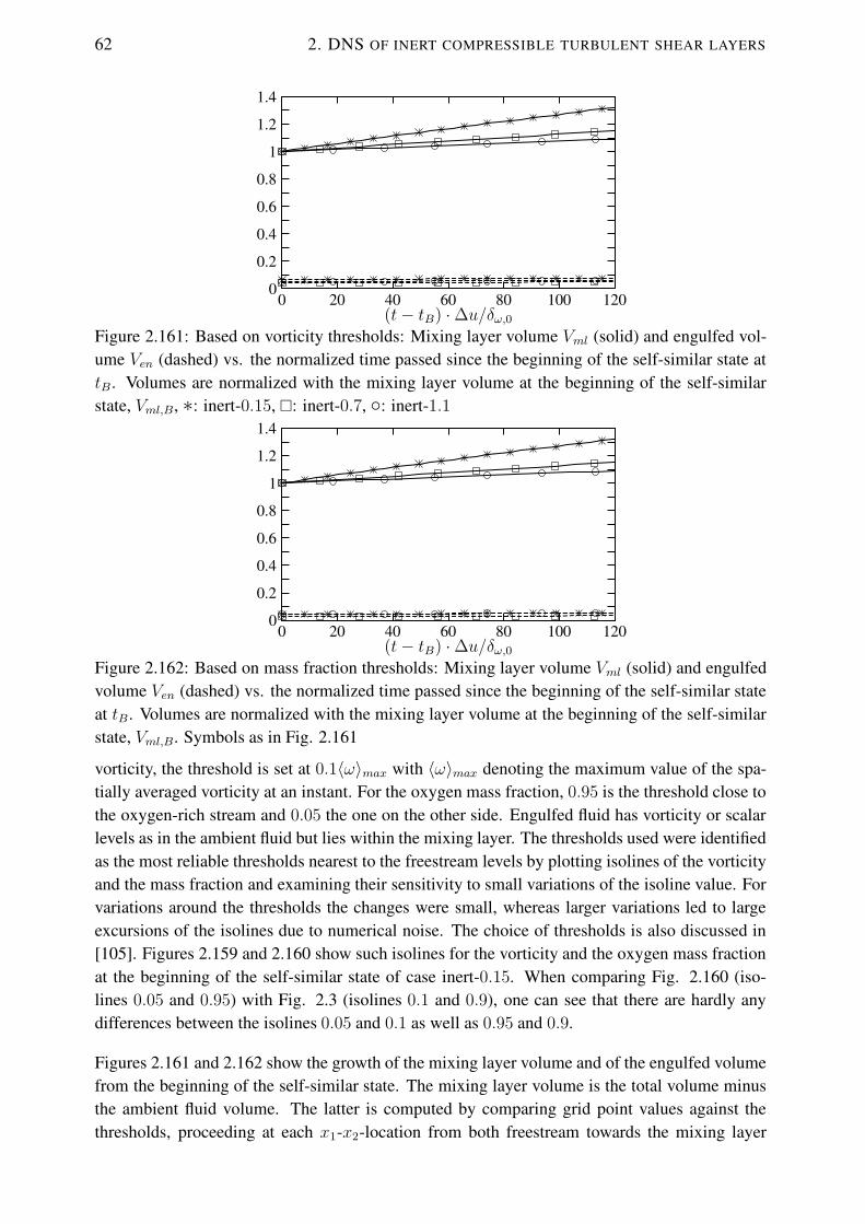
62 2. DNS OF INERT COMPRESSIBLE TURBULENT SHEAR LAYERS
(t− tB) ·∆u/δω,0120100806040200
1.4
1.2
1
0.8
0.6
0.4
0.2
0
Figure 2.161: Based on vorticity thresholds: Mixing layer volume Vml (solid) and engulfed vol-ume Ven (dashed) vs. the normalized time passed since the beginning of the self-similar state attB . Volumes are normalized with the mixing layer volume at the beginning of the self-similarstate, Vml,B, ∗: inert-0.15, �: inert-0.7, ◦: inert-1.1
(t− tB) ·∆u/δω,0120100806040200
1.4
1.2
1
0.8
0.6
0.4
0.2
0
Figure 2.162: Based on mass fraction thresholds: Mixing layer volume Vml (solid) and engulfedvolume Ven (dashed) vs. the normalized time passed since the beginning of the self-similar stateat tB . Volumes are normalized with the mixing layer volume at the beginning of the self-similarstate, Vml,B. Symbols as in Fig. 2.161
vorticity, the threshold is set at 0.1〈ω〉max with 〈ω〉max denoting the maximum value of the spa-tially averaged vorticity at an instant. For the oxygen mass fraction, 0.95 is the threshold close tothe oxygen-rich stream and 0.05 the one on the other side. Engulfed fluid has vorticity or scalarlevels as in the ambient fluid but lies within the mixing layer. The thresholds used were identifiedas the most reliable thresholds nearest to the freestream levels by plotting isolines of the vorticityand the mass fraction and examining their sensitivity to small variations of the isoline value. Forvariations around the thresholds the changes were small, whereas larger variations led to largeexcursions of the isolines due to numerical noise. The choice of thresholds is also discussed in[105]. Figures 2.159 and 2.160 show such isolines for the vorticity and the oxygen mass fractionat the beginning of the self-similar state of case inert-0.15. When comparing Fig. 2.160 (iso-lines 0.05 and 0.95) with Fig. 2.3 (isolines 0.1 and 0.9), one can see that there are hardly anydifferences between the isolines 0.05 and 0.1 as well as 0.95 and 0.9.
Figures 2.161 and 2.162 show the growth of the mixing layer volume and of the engulfed volumefrom the beginning of the self-similar state. The mixing layer volume is the total volume minusthe ambient fluid volume. The latter is computed by comparing grid point values against thethresholds, proceeding at each x1-x2-location from both freestream towards the mixing layer

RESULTS AND ANALYSIS 63
until locations where the thresholds were crossed. All these locations constitute the ambient fluidvolume. The engulfed volume consists of the grid points within the mixing layer, the values ofwhich are below the threshold. The rest of the mixing layer can be considered the mixed volume.Figure 2.161 shows the curves based on the vorticity threshold (0.1〈ω〉max) and Fig. 2.162 theones based on the mass fraction thresholds (0.05 and 0.95). The conclusions from the two figuresare the same: Both, mixing layer volume and engulfed volume, grow during the simulations. Thegrowth rate of the mixing layer volume reduces with increasing Mc, and the growth rate of theengulfed volume is smaller than the one of the mixing layer volume at all Mc. Both growth ratesare nearly constant throughout the self-similar state. In total, the engulfed volume is just a verysmall part of the mixing layer volume, around 6% for Mc = 0.15. This percentage even reduceswith increasing Mc (5% for Mc = 0.7 and 4% for Mc = 1.1) which indicates that compressibilitysuppresses engulfment.
Visual thickness The visual thickness δvis is the distance in transverse direction between thetwo points where 〈ω〉 = 0.1〈ω〉max or, alternatively, where the spatially averaged mass fractionhas the values 0.05 and 0.95. Its temporal development and the temporal development of a thick-ness computed from the mixing layer volume, δvol = Vml/ (L1 · L2), is shown in Figs. 2.163(based on vorticity thresholds) and 2.164 (based on mass fraction thresholds) for the self-similarstate. At all convective Mach numbers, the growth rates of both thicknesses are nearly linear andequal. They decrease with increasing Mach number which is in agreement with other measure-ments of the mixing layer thickness, e.g. the momentum and vorticity thicknesses and with theLangley curve (cf. Sect. 2.4.2).
At all convective Mach numbers, the visual thickness is larger than the thickness derived fromthe mixing layer volume. This is due to intermittent outward ejections of vortical fluid fromthe mixing layer and can be understood when taking into account the different ways by whichthe two thicknesses are computed: In a laminar mixing layer, both thicknesses would coincideand represent the boundary of the mixing layer. In a turbulent flow, when there are a few ejec-tions from the turbulent region to the non-turbulent surrounding, the mean boundary, computedby averaging the mixing layer volume, will move slightly. The shift is not very large as onlyfew ejections are present. However, the ejections consist of core fluid and carry therefore highlevels of vorticity and concentration. The consequence is that even though these events are notfrequent, the average vorticity and concentration profiles are affected considerably and the visualthickness which is obtained from these profiles is larger than the thickness derived from the mix-ing layer volume. This intermittency effect is more pronounced when using vorticity thresholds(Fig. 2.163) to determine the mixing layer boundary than when using mass fraction thresholds(Fig. 2.164). Figures 2.163 and 2.164 also show that the higher the Mach number, the closer arethe visual thickness and the thickness computed from the mixing layer volume which indicates adecrase of intermittency.
Measurement of densities Figure 2.165 shows the density of the mixing layer, the density ofthe engulfed volume and the density of the mixed volume which are determined based on the vor-ticity threshold. It can be seen that the mixing layer density and the density of the mixed volumedecrease with increasing compressibility which is due to heating by dissipation. Shocklets, even

64 2. DNS OF INERT COMPRESSIBLE TURBULENT SHEAR LAYERS
(t− tB) ·∆u/δω,0120100806040200
1.4
1.3
1.2
1.1
1
0.9
0.8
Figure 2.163: Based on vorticity thresholds: Thickness computed from mixing layer volume δvol(solid) and visual thickness δvis (dashed). Thicknesses are normalized by the visual thickness atthe beginning of the self-similar state, δvis,B. Symbols as in Fig. 2.161
(t− tB) ·∆u/δω,0120100806040200
1.4
1.3
1.2
1.1
1
0.9
0.8
Figure 2.164: Based on mass fraction thresholds: Thickness computed from mixing layer volumeδvol (solid) and visual thickness δvis (dashed). Thicknesses are normalized by the visual thicknessat the beginning of the self-similar state, δvis,B . Symbols as in Fig. 2.161
though present in the mixing layer at Mc = 1.1 (cf. Sect. 2.4.4.4), are not frequent enough to risethe density again.
The density of the engulfed volume is always higher than the density of the mixing layer, since itenters the mixing layer from the non-turbulent region where no heating due to dissipation takesplace. However, the fact that the difference between the reference density ρ0 and the density ofthe engulfed volume increases with increasing convective Mach number shows that dissipativeheating is not completely absent within the engulfed volume.
For all convective Mach numbers, the density of the mixed volume is lower than the density ofthe complete mixing layer which includes also the engulfed volume. Since the density differencebetween the engulfed volume and the mixed volume increases with compressibility, the differencebetween the mixed volume density and the mixing layer density increases also.
Figure 2.166 shows the corresponding density curves whereby the regions are determined with thehelp of the mass fraction thresholds. It can be seen that the curves of the engulfed volume are allvery close to the reference density ρ0 now. This demonstrates that the two threshold definitions arenot fully equivalent and that dissipative heating has less effect on the engulfed volume determinedby the mass fraction criteria than on the one determined by the vorticity criteria.
In both figures, the density of the engulfed volume of the mixing layer at Mc = 1.1 has a rising

RESULTS AND ANALYSIS 65
(t− tB) ·∆u/δω,0120100806040200
1.1
1
0.9
0.8
Figure 2.165: Based on vorticity thresholds: Mixing layer density ρml/ρ0 (solid), density of theengulfed volume, ρen/ρ0 (dashed), and density of the mixed volume, ρmix/ρ0 (dotted), vs. thenormalized time passed since the beginning of the self-similar state at tB . Symbols as in Fig.2.161
(t− tB) ·∆u/δω,0120100806040200
1.1
1
0.9
0.8
Figure 2.166: Based on mass fraction thresholds: Mixing layer density ρml/ρ0 (solid), densityof the engulfed volume, ρen/ρ0 (dashed), and density of the mixed volume, ρmix/ρ0 (dotted), vs.the normalized time passed since the beginning of the self-similar state at tB . Symbols as in Fig.2.161tendency and even exceeds the reference density in Fig. 2.166. It is assumed that this is dueto compression processes like shocklets (cf. Sect. 2.4.4.4) that within the engulfed volume - incontrast to the complete mixing layer - overcome the density decrease by dissipation.
Particle statistics During the self-similar state pathlines of fluid particles were computed. Todo so, the velocity components at the locations of the particles were integrated every time step,and the new positions of the particles were determined. The interpolation of the velocity fieldfrom the grid points to the locations of the particles was performed with a third order Taylorseries 13-point scheme proposed by Yeung & Pope [191]. This scheme requires data at staggeredgrid points which were obtained by spectral (exact) interpolation in the periodic x1- and x2-directions and by sixth-order explicit interpolation in the x3-direction [99]. In addition to thevelocity components, the vorticity and the scalar mass fraction at the locations of the particleswere also computed.
The initialization of the particles is done at times when the mixing layers are already turbulentbut have not yet reached the self-similar state. Table 2.6 lists the number of the particles, thetimes at which they are initialized and their initial transverse positions for all test cases. Particles

66 2. DNS OF INERT COMPRESSIBLE TURBULENT SHEAR LAYERS
Figure 2.167: Particle tracks in the upper half of the computational domain during the self-similarstate of inert-0.7were placed at every 12th grid point in the x1- and x2-directions and at every 8th point in thex3-intervals that are mentioned in table 2.6. These intervals were chosen such that initially nearlyall particles are situated outside the mixing layer (defined by the vorticity criteria) but close to itsedges.
In the following, it is investigated how the vorticity and the concentration grow along pathlines,examples of which are shown in Fig. 2.167. It was found by Mathew and Basu [105] that ina circular mixing layer, the growth of vorticity and concentration occurs close to the turbulentboundary, and that they are often relatively fast processes. To determine if a particle has enteredthe mixing layer, a lower and an upper threshold for the vorticity and the mass fraction are used.This also captures a transition stage between the non-turbulent and turbulent flow which wouldnot be the case when using just one threshold, i.e. a sharp cut-off. The lower threshold for thevorticity is at 0.1〈ω〉max, the upper one at 0.2〈ω〉max. For the scalar value (oxygen mass fraction),the thresholds are 0.95 and 0.9 on the oxygen-rich side and 0.05 and 0.1 on the other.
In Table 2.7, statistical quantities for the particles during the self-similar state are listed. Thefirst two rows are displacements in the direction of the mean shear between the locations whencrossing the lower (subscript l) and upper (subscript u) thresholds. The values obtained with thevorticity thresholds have the index ω, while the ones obtained with the mass fraction thresholdshave the index Y . For normalization, δvis at the time tl at which the lower threshold was crossedhas been used. The third and the fourth rows are the elapsed times between the crossing of thelower and the upper thresholds, and the last two rows are the times between the crossing of thevorticity and the mass fraction thresholds. The times are normalized by tvis = δvis (tl) /∆u. Inthe last two rows, a δvis (tl) has been used, which is the averaged value of the one determinedwith the vorticity and the one determined with the mass fraction. Only particles that are outsidethe visual thickness of the shear layer at the beginning of the self-similar period are considered.These are 14970 particles for case inert-0.15, 15764 for case inert-0.7 and 13335 for case inert-1.1. The sample size gives the number of particles which among these have crossed the respectivethresholds and are therefore used to compute the respective statistical quantity.
Comparing the mean values in the first four lines of each test case with its considerably largermaximum, one can see that most of the threshold crossings occur quite fast and close to theboundary of the mixing layer. The means in the last two lines of each test case are positive which
Table 2.6: Particle parameters: NP particles are initialized at τω,PB. They are situated initiallybetween x3 = x3,P1 and x3,P2 and between x3 = x3,P3 and x3,P4
NP τω,PB x3,P1/δω,0 x3,P2/δω,0 x3,P3/δω,0 x3,P4/δω,0
inert-0.15 20480 209 -23.81 -11.19 10.68 23.30inert-0.7 24576 404 -28.52 -13.55 13.21 28.18inert-1.1 20480 843 -37.27 -24.82 21.96 34.41

RESULTS AND ANALYSIS 67
is suggesting that the growth of vorticity occurs faster than the growth of mass fraction. This canbe explained by the fact that the flow is governed by the velocity field from which the vorticityis computed. In summary, the statistics show that the growth of vorticity and concentration is arelatively fast process which is occuring close to the boundary of the turbulent region. This isconsistent with the findings of [105] for the circular mixing layer and leads to the conclusion thatnibbling, rather than engulfment is the process by which the mixing layer is growing.
At higher convective Mach number the fluid particles that start entering the mixing layer stayclose to its edges for a longer time and are carried along before they penetrate inside. This canbe seen from the elapsed times between the crossing of the lower and upper thresholds which arelarger for the higher convective Mach numbers. In contrast to the times, the displacements in thefirst two lines of each test case do not change much with compressibility. While the particles athigher Mc are convected downstream near the edges of the mixing layer they are slowed downto a variable degree. This becomes clear when looking at the pdf of the local Mach numberassembled at the time the upper vorticity threshold is crossed (Fig. 2.168) While it is narrowwith a mean close to 0.15 when Mc = 0.15, the distribution at Mc = 0.7 is much broader andextends from slightly above 0.7 down to about 0.2. The whole mechanism can be seen as somekind of resistance that the compressible mixing layer as compared to the incompressible mixinglayer offers towards fluid particles before they are penetrating the mixing layer. Entrainment,the process of ambient fluid acquiring vorticity, takes place at the very periphery of the turbulentregion. Then, the growth rate is diminished as fluid packets spend a longer period at the turbulence
Table 2.7: Statistics of displacements and elapsed times for growth of vorticity and mixture frac-tion along particle pathlines
Sample size Mean Max Min
inert-0.15 |x3,ωu − x3,ωl| /δvis (tl) 4220 0.0250 0.5201 0|x3,Y u − x3,Y l| /δvis (tl) 3875 0.0337 0.5878 0(tωu − tωl) /tvis 4220 0.4696 9.1722 0(tY u − tY l) /tvis 3875 0.6144 8.6643 0(tY l − tωl) /tvis 4728 0.0301 5.4441 -5.8458(tY u − tωu) /tvis 3636 0.1419 6.3473 -9.1722
inert-0.7 |x3,ωu − x3,ωl| /δvis (tl) 12760 0.0290 0.6667 0|x3,Y u − x3,Y l| /δvis (tl) 11792 0.0423 0.6769 0(tωu − tωl) /tvis 12760 0.8359 17.8751 0(tY u − tY l) /tvis 11792 1.1986 19.4045 0(tY l − tωl) /tvis 13333 0.3018 9.8935 -13.2233(tY u − tωu) /tvis 11561 0.6607 17.7959 -17.7959
inert-1.1 |x3,ωu − x3,ωl| /δvis (tl) 5364 0.0205 0.3878 0|x3,Y u − x3,Y l| /δvis (tl) 2909 0.0362 0.5031 0(tωu − tωl) /tvis 5364 0.7808 9.8476 0(tY u − tY l) /tvis 2909 1.2193 9.8476 0(tY l − tωl) /tvis 5299 0.5850 7.9822 -8.2881(tY u − tωu) /tvis 2841 0.9067 9.8476 9.4413

68 2. DNS OF INERT COMPRESSIBLE TURBULENT SHEAR LAYERS
M
1.41.210.80.60.40.20
181614121086420
Figure 2.168: Pdfs of the local Mach number magnitude at the time when the particles are cross-ing the upper vorticity threshold. Symbols as in Fig. 2.161
boundary becoming a part of the turbulence. The lowered entrainment with compressibility goesin hand with the structural changes that are experiencing the turbulence interfaces with increasingMc, which result in them being smoother than at low Mc (cf. next paragraph).
Fractal nature of the mixing layer interface It is of interest to see how the geometrical prop-erties of the turbulent-nonturbulent interfaces of the mixing layer vary with compressibility andto see whether these changes can be related with the changes noticed concerning the entrainment.One question that arises in this context is whether the interfaces are fractal. Sreenivasan & Men-eveau [173] performed measurements in turbulent shear flow and came to the conclusion thatseveral aspects of turbulence, among others this very interface, can be described roughly by frac-tals. Mathew & Basu [105] argued that, if this were the case, the entrainment flux estimated onlarge scales could equal that summed from the actual small-scale processes due to the equilibriumacross scales that is usually obtained in the self-preserving canonical shear layer.
Figures 2.169 to 2.174 show some of the interfaces that are investigated in the following. It isclearly visible how the dominant scales of the vorticity isosurfaces and the mass fraction iso-surfaces increase with increasing Mc (cf. also Sect. 2.4.1). Close examination reveals that thesurface has small, evenly distributed protrusions into the non-turbulent region at the lower convec-tive Mach number, while at higher Mc the protrusions are thicker. In total, the observed changesin the dominant interface scales are consistent with the reduced entrainment and mixing layergrowth at higher Mach numbers when the process is small-scale and occurs at the interface.
A quantitative characterization of the turbulence interface is obtained by measuring its fractaldimension. The evaluation of the fractal dimensions of the mixing layers is done in the followingby finding the dimension D2 of this interface, determined by vorticity or by mass fraction, within
Table 2.8: Fractal dimensions D of isosurfaces determined from the slopes of the curves in Figs.2.175 to 2.176 and corresponding ones for ω = 0.2〈ω〉max and Y = 0.9
ω = 0.2〈ω〉max ω = 0.1〈ω〉max Y = 0.9 Y = 0.95
inert-0.15 2.56 2.41 2.41 2.35inert-0.7 2.64 2.45 2.40 2.31inert-1.1 2.68 2.49 2.46 2.37
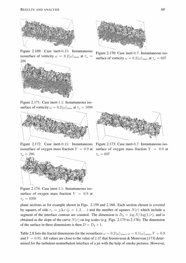
RESULTS AND ANALYSIS 69
Figure 2.169: Case inert-0.15: Instantaneousisosurface of vorticity ω = 0.2〈ω〉max at τω =
286
Figure 2.170: Case inert-0.7: Instantaneous iso-surface of vorticity ω = 0.2〈ω〉max at τω = 697
Figure 2.171: Case inert-1.1: Instantaneous iso-surface of vorticity ω = 0.2〈ω〉max at τω = 1098
Figure 2.172: Case inert-0.15: Instantaneousisosurface of oxygen mass fraction Y = 0.9 atτω = 286
Figure 2.173: Case inert-0.7: Instantaneous iso-surface of oxygen mass fraction Y = 0.9 atτω = 697
Figure 2.174: Case inert-1.1: Instantaneous iso-surface of oxygen mass fraction Y = 0.9 atτω = 1098
plane sections as for example shown in Figs. 2.159 and 2.160. Each section chosen is coveredby squares of side rj = j∆x (j = 1, 2, . . .) and the number of squares N(r) which include asegment of the interface contour are counted. The dimension is D2 = logN/ log(1/r), and isobtained as the slope of the curve N(r) on log scales (e.g. Figs. 2.175 to 2.176). The dimensionof the surface in three dimensions is then D = D2 + 1.
Table 2.8 lists the fractal dimensions for the isosurfaces ω = 0.2〈ω〉max, ω = 0.1〈ω〉max, Y = 0.9
and Y = 0.95. All values are close to the value of 2.37 that Sreenivasan & Meneveau [173] deter-mined for the turbulent-nonturbulent interface of a jet with the help of smoke pictures. However,

70 2. DNS OF INERT COMPRESSIBLE TURBULENT SHEAR LAYERS
δω,0/r
N
10.1
100000
10000
1000
Figure 2.175: Number of squares N covering the interface ω = 0.1〈ω〉max vs. δω,0/r, averagedover the self-similar state, solid: inert-0.15, dashed: inert-0.7, dotted: inert-1.1
δω,0/r
N
10.1
100000
10000
1000
Figure 2.176: Number of squares N covering the interface Y = 0.95 vs. δω,0/r, averaged overthe self-similar state, solid: inert-0.15, dashed: inert-0.7, dotted: inert-1.1
small differences can be noticed between the different interfaces that are listed in table 2.8 andbetween the different convective Mach numbers. The fractal dimensions generally decrease whenchosing the interface closer to the free-stream value, i.e. chosing Y = 0.95 instead of Y = 0.9
and ω = 0.1〈ω〉max instead of ω = 0.2〈ω〉max, and the fractal dimensions of the vorticity iso-surfaces are higher than the ones of the mass fraction isosurfaces due to less intermittency of thelatter one. With increasing compressibility, the fractal dimension of the mixing layer interfacesdefined by vorticity increases. For the mixing layer interfaces defined by mass frations, the fractaldimension decreases when rising Mc from 0.15 to 0.7, but increases again for Mc = 1.1. The fallbetween Mc = 0.15 and Mc = 0.7 is consistent with a decrease in entrainment and shear layergrowth rate. The increase at Mc = 1.1 may be due to rapid changes in scale in the infrequentindentations, but the generally smoother boundary is nonetheless consistent with the observedfurther decrease in growth rate and entrainment by processes at the turbulence boundaries. Thissmoothening of the boundary could also account for the observed tapering off of the fall in growthrate at Mc ≈ 1.1.
2.4.4.4 Shocklets
When monitoring the temporal development of the normalized, maximum pressure gradient dur-ing the simulations with different convective Mach numbers (Fig. 2.177), one notices that it is

RESULTS AND ANALYSIS 71
τω
√(∂p/∂xi)
2·δ
ω,0/〈p〉av
180016001400120010008006004002000
9876543210
Figure 2.177: Temporal development of the maximum pressure gradient, normalized by〈p〉av/δω,0, ∗: inert-0.15, �: inert-0.7, ◦: inert-1.1
much higher for the mixing layer at Mc = 1.1 than for the ones at smaller convective Machnumber. This is particularly the case during the initial development, but also later during theself-similar state where the peak values of the maximum pressure gradient of case inert-1.1 areabout double the values of case inert-0.7. In Figure 2.177, the pressure gradient is normalizedby 〈p〉av, the box-averaged pressure, temporally averaged over the self-similar state. The highpressure gradients of the inert-1.1 case suggest the existence of so-called ’eddy shocklets’, whichare small shocklets that are associated with turbulent eddies.
Eddy shocklets were first observed in two- and three-dimensional simulations of isotropic turbu-lence [97, 127]. In two-dimensional simulations of mixing layers, shocklets were found to occurat convective Mach numbers higher than 0.7 [98, 159]. However, in 3D, the flow has anotherdimension in which it can change direction and thus avoid high pressure regions that are due tovortical motions. Therefore, shocks were only observed at considerably higher convective Machnumbers than in 2D, e.g. Mc = 1.2 [182] or 1.25 and larger [115]. Other authors [63], foundshocklets only from Mc = 1.54, which they attribute on one hand to the influence of differentinitial conditions or the finite box size and on the other to the lack of a definitive criterion of whena pressure disturbance is really a shock. Experiments have also revealed the presence of shockletsin a counterflowing supersonic shear layer [125].
In order to detect possible shocklets in the simulation inert-1.1, locations with high pressuregradients and strongly negative dilatation are investigated in more detail, and it is checked whetherthe shock jump (Rankine-Hugeniot) relations apply. However, as Freund et al. [63] point out, theyare not expected to hold exactly since they are derived for an ideal gas, and the shocklets in thesimulation have a finite thickness and are not steady. However, despite these deficiencies, theseand others authors [12], were able to verify the shock jump relations with an accuracy between 3
and 30 %.
The first structure that is investigated in the following occurs at τω = 1023, which is shortly afterthe beginning of the self-similar state. The maximum pressure gradient at this instance is found atx1 = 0.30L1, x2 = 0.30L2, x3 = 0.32L3 and has an inclination of 6.4◦ with respect to the x1-x2-plane and an inclination of 10.3◦ with respect to the x1-x3-plane. Since these angles are small, theshock jump relations are verified with the help of the values along a line, parallel to the x1-axis,through the location of the maximum pressure gradient. Figures 2.178 to 2.179 show the pressuregradient, the pressure, the density and the temperature along this line. In these figures, everyfourth grid point is shown which demonstrates that the shock is well resolved by five grid-points.

72 2. DNS OF INERT COMPRESSIBLE TURBULENT SHEAR LAYERS
x1/L1√(∂p/∂xi)
2·δ
ω,0/〈p〉av
0.340.320.30.280.260.240.220.2
0.8
0.7
0.6
0.5
0.4
0.3
0.2
0.1
0
Figure 2.178: Case inert-1.1: Pressure gradi-ent normalized by 〈p〉av/δω,0 on a line paral-lel to the x1-axis through x2 = 0.30L2 andx3 = 0.32L3 at τω = 1023. Every 4th gridpoint is shown
x1/L1
p/〈p〉 av
0.340.320.30.280.260.240.220.2
1.2
1.15
1.1
1.05
1
0.95
0.9
0.85
0.8
Figure 2.179: Case inert-1.1: Pressure normal-ized by 〈p〉av on a line parallel to the x1-axisthrough x2 = 0.30L2 and x3 = 0.32L3 atτω = 1023. Every 4th grid point is shown
x1/L1
ρ/ρ
0
0.340.320.30.280.260.240.220.2
1.15
1.1
1.05
1
0.95
0.9
0.85
0.8
0.75
Figure 2.180: Case inert-1.1: Density in x1-direction normalized by ρ0 on a line parallelto the x1-axis through x2 = 0.30L2 and x3 =
0.32L3 at τω = 1023. Every 4th grid point isshown
x1/L1
T/T
0
0.340.320.30.280.260.240.220.2
1.25
1.2
1.15
1.1
1.05
1
0.95
0.9
Figure 2.181: Case inert-1.1: Temperaturenormalized by T0 on a line parallel to the x1-axis through x2 = 0.30L2 and x3 = 0.32L3 atτω = 1023. Every 4th grid point is shown
Therefore, no Gibbs-phenomenon due to under-resolution occurs. Computing ratios with theminimum and maximum values to the left and right side of the shock at x1 = 0.30L1, one obtains:pmax/pmin = 1.398, ρmax/ρmin = 1.296 and Tmax/Tmin = 1.089. With the shock relations foran ideal gas (γ = 1.4), one would obtain a density ratio of 1.269 and a temperatur ratio of 1.102
for the same pressure ratio which is a difference of less than 2.5 % from the actual values. Thecorresponding upstream normal shock number would be 1.158. However, when checking it, onehas to take into account that the shock is not necessarily stationary with respect to the grid andthat its speed is unknown. According to Blaisdell et al. [12], it can be checked anyway with thehelp of the velocity jump across the shock, ua− ub, which is Galilean invariant and consequentlyindependent of the shock velocity. When the shock does not contain any mass, i.e. is very thin, the
x1/L1
∂ui/∂xi·δω,0/∆
u
0.340.320.30.280.260.240.220.2
0.025
0.02
0.015
0.01
0.005
0
-0.005
-0.01
-0.015
Figure 2.182: Case inert-1.1: Dilatation nor-malized by ∆u/δω,0 on a line parallel to thex1-axis through x2 = 0.30L2 and x3 = 0.32L3
at τω = 1023. Every 4th grid point is shown
x1/L1
√ω
2 i·δ
ω,0/∆
u
0.340.320.30.280.260.240.220.2
1.6
1.4
1.2
1
0.8
0.6
0.4
0.2
0
Figure 2.183: Case inert-1.1: Vorticity nor-malized by ∆u/δω,0 on a line parallel to thex1-axis through x2 = 0.30L2 and x3 = 0.32L3
at τω = 1023. Every 4th grid point is shown

RESULTS AND ANALYSIS 73
velocity jump remains even uninfluenced by a shock acceleration. If va and vb are the velocitiesrelative to the moving shock, it therefore holds that ua − ub = va − vb = caM
rela − cbM rel
b andthat M rel
b is a known function of M rela (e.g. [51]):
(M rel
b
)2=
1 + [(γ − 1) /2](M rel
a
)2
γ (M rela )2 − [(γ − 1) /2]
(2.92)
With ua, the velocity in the direction of the maximum pressure gradient (normal to the shock)evaluated at the location of the minimum pressure and ub, the velocity in the same direction atthe location of the maximum pressure, as well as the correspoding speeds of sound, ca and cb, aMach number of 1.147 is obtained which is less than 1 % difference from the previously obtainedvalue. However, the next example will show that such a high precision is rather incidential andcannot generally be expected since, among other deficiencies, the states on both sides of the shockare not uniform . Nevertheless, shocklets seem to be present in the mixing layer at Mc = 1.1.Figure 2.182 shows the dilatation along the line along which the shock jump conditions havebeen verified. Next the expected minimum in the dilatation at the location where the pressurerises steeply, there is an even more marked dilatation maximum on the right side of the shockletwhere the pressure falls. The peak of the vorticity, shown in figure 2.183, is much larger than themagnitude of the dilatation extrema, which has also been noticed by [63].
The other compressible structure, that is further investigated in the following, manifests thehighest pressure gradient during the self-similar state. It is found at x1 = 0.02L2, x2 = 0.38,x3 = 0.31L3 and τω = 1295. The maximum pressure gradient has an inclination of 4.93◦ withrespect to the x1-x2-plane and an inclination of 38.5◦ with respect to the x1-x3-plane. Therefore,it is appropriate to verify the shocklet jump conditions on a line in the x1-x2-plane which has aninclination of 45◦ with respect to the x1-x3-plane. Figures 2.184 to 2.187 show thermodynamicquantities along this line on which the shocklet is situated at (x2
1 + x22)
0.5= 0.093 (L2
1 + L22)
0.5.It is found that pmax/pmin = 1.835, ρmax/ρmin = 1.874 and Tmax/Tmin = 1.119. With theshocklet relations for an ideal gas (γ = 1.4), one would obtain with the same pressure ratioρmax/ρmin = 1.533, which is a difference of 22 % to the actual value and Tmax/Tmin = 1.197,which is 6.5 % difference. The upstream normal Mach number would be 1.310. Again, this Machnumber can be verified with the help of the velocity jump that is the same as in a moving refer-ence frame. With the values ua, ub, ca and cb inserted in Eq. (2.92), one obtaines M1,rel = 1.137,
(x21 + x2
2)0.5/ (L2
1 + L22)
0.5√(∂p/∂xi)
2·δ
ω,0/〈p〉av
0.260.240.220.20.180.160.14
1.2
1
0.8
0.6
0.4
0.2
0
Figure 2.184: Case inert-1.1: Pressure gradi-ent normalized by 〈p〉av/δω,0 on a line throughx1 = 0.02L2, x2 = 0.38 and x3 = 0.31L3 (inx1-x2-plane, inclined 45◦ to the x1-x3-plane)at τω = 1295. Every 4th grid point is shown
(x21 + x2
2)0.5/ (L2
1 + L22)
0.5
p/〈p〉 av
0.260.240.220.20.180.160.14
1.4
1.3
1.2
1.1
1
0.9
0.8
0.7
0.6
Figure 2.185: Case inert-1.1: Pressure normal-ized by 〈p〉av on a line through x1 = 0.02L2,x2 = 0.38 and x3 = 0.31L3 (in x1-x2-plane,inclined 45◦ to the x1-x3-plane) at τω = 1295.Every 4th grid point is shown

74 2. DNS OF INERT COMPRESSIBLE TURBULENT SHEAR LAYERS
(x21 + x2
2)0.5/ (L2
1 + L22)
0.5
ρ/ρ
0
0.260.240.220.20.180.160.14
1.2
1.1
1
0.9
0.8
0.7
0.6
0.5
Figure 2.186: Case inert-1.1: Density in x1-direction normalized by ρ0 on a line throughx1 = 0.02L2, x2 = 0.38 and x3 = 0.31L3 (inx1-x2-plane, inclined 45◦ to the x1-x3-plane)at τω = 1295. Every 4th grid point is shown
(x21 + x2
2)0.5/ (L2
1 + L22)
0.5
T/T
0
0.260.240.220.20.180.160.14
1.26
1.24
1.22
1.2
1.18
1.16
1.14
1.12
1.1
1.08
Figure 2.187: Case inert-1.1: Temperaturenormalized by T0 on a line through x1 =
0.02L2, x2 = 0.38 and x3 = 0.31L3 (in x1-x2-plane, inclined 45◦ to the x1-x3-plane) atτω = 1295. Every 4th grid point is shown on
(x21 + x2
2)0.5/ (L2
1 + L22)
0.5
∂ui/∂xi·δ
ω,0/∆
u
0.260.240.220.20.180.160.14
350030002500200015001000
5000
-500-1000-1500-2000
Figure 2.188: Case inert-1.1: Dilatation nor-malized by ∆u/δω,0 on a line through x1 =
0.02L2, x2 = 0.38 and x3 = 0.31L3 (in x1-x2-plane, inclined 45◦ to the x1-x3-plane) atτω = 1295. Every 4th grid point is shown
(x21 + x2
2)0.5/ (L2
1 + L22)
0.5
√ω
2 i·δ
ω,0/∆
u
0.260.240.220.20.180.160.14
140000
120000
100000
80000
60000
40000
20000
0
Figure 2.189: Case inert-1.1: Vorticity nor-malized by ∆u/δω,0 on a line through x1 =
0.02L2, x2 = 0.38 and x3 = 0.31L3 (in x1-x2-plane, inclined 45◦ to the x1-x3-plane) atτω = 1295. Every 4th grid point is shown
which is a difference of 13 % to the previously estimated value. Therefore, the verification of theRankine-Hugeniot relations can be considered successful and the compressible structure can becalled a shocklet. Figures 2.188 and 2.189 show the dilatation and the vorticity and confirm theobservations already made: While there is a local minimum of the dilatation at the location ofthe shocklet, a local maximum is situated right next to it. A vorticity maximum, which is muchlarger in magnitude than the dilatation extrema, is found close to the shocklet.
Figure 2.190 presents the instantaneous dilatation field together with the pressure isolines in the
Figure 2.190: Case inert-1.1: Instantaneousdilatation field and pressure isolines, x1-x2-plane through x3 = 0.49L3 at τω = 1295.Dilatation is normalized by δω,0/∆u
Figure 2.191: Case inert-1.1: Instantaneousmagnitude of vorticity and velocity vectors,x1-x2-plane through x3 = 0.49L3 at τω =
1295. Vorticity is normalized by δω,0/∆u

RESULTS AND ANALYSIS 75
Figure 2.192: Case inert-1.1: Instantaneousdilatation field and pressure isolines, x1-x3-plane through x2 = 0.59L2 at τω = 1295.Scale as in Fig. 2.190
Figure 2.193: Case inert-1.1: Instantaneousmagnitude of vorticity and velocity vectors,x1-x3-plane through x2 = 0.59L2 at τω =
1295. Scale as in Fig. 2.191
Figure 2.194: Case inert-1.1: Instantaneous di-latation field and pressure isolines, x2-x3-planethrough x1 = 0.03L1 at τω = 1295. Scale as inFig. 2.190
Figure 2.195: Case inert-1.1: Instantaneousmagnitude of vorticity and velocity vectors, x2-x3-plane through x1 = 0.03L1 at τω = 1295.Scale as in Fig. 2.191
x1-x2-plane in which the shocklet is situated. The shocklet is on the left side of the section whichis shown. It can be seen how close the dilatation minimum at the location of the shocklet and amaximum are situated next to each other. Fig. 2.191 shows the velocity vectors and the vorticityfield in the same part of the domain. The change of velocity direction by the shocklet as well as thevortical structures that are causing it are clearly visible. Figures 2.192 and 2.193 show x1-x3-cutsthrough the shocklet. In this view, it is only visible as a kind of point (in the middle on the far leftside of the figure) and one could think it had a pencil-like shape. However, the other figures (e.g.Figs. 2.190 and 2.191) reveal its curved nature. Blaisdell et al. [12] suggested a mechanism forthe formation of shocklets based on their observation from instantaneous pressure and vorticityfields: Most of the shocklets in their simulations seem to be caused by vortex motions whichtransport fluid in the direction of the mean shear. This brings together high-speed and low-speedfluid and the collision caused strong compressions and shock waves. In our simulation such

76 2. DNS OF INERT COMPRESSIBLE TURBULENT SHEAR LAYERS
Figure 2.196: Case inert-1.1: Instantaneousdilatation field, x1-x3-plane through x2 =
0.59L2 at τω = 1295. Dilatation is normal-ized by δω,0/∆u
Figure 2.197: Case inert-1.1: Instantaneouspressure gradient field, x1-x3-plane throughx2 = 0.59L2 at τω = 1295. Pressure gradi-ent is normalized by δω,0/〈p〉av
vortical motions, which are transporting fluid in the direction of the shear, are visible in Fig.2.193, too. Figs. 2.194 and 2.195, x2-x3-cuts, reveal them even more clearly. The superpositionof the downwashs of various vortical structures cause sudden changes of the velocity directionand lead to the formation of the shocklet.
Finally, Figs. 2.196 and 2.197 show the complete computational domain. The recently investi-gated shocklet is visible to the extreme left. The figures demonstrate that neither extremely highpressure gradients nor dilatation minima are very frequent. Therefore, the shocklets in the simu-lation inert-1.1 do not seem to play a major role for the overall dynamics which is confirmed bythe fact that the pressure dilatation is small even at Mc = 1.1 and the decreasing tendency of thedilatational dissipation lingers between Mc = 0.7 and Mc = 1.1 despite the presence of shocklets(cf. Sect. 2.4.4.1).
2.5 Summary and conclusions
In this chapter, DNS of turbulent, temporally evolving, inert mixing layers at different convectiveMach numbers (Mc = 0.15, 0.7 and 1.1) - equivalent to different levels of compressibility - havebeen described and analyzed. The particular focus of the study is on the effects that compressibil-ity has on the turbulence in general, on scalar mixing and entrainment. All simulations have beenperformed over a sufficiently long period of time which allowed the attainment of a self-similarstate with constant momentum thickness growth rates. Statistics have been taken over this stateduring which profiles of adequately normalized flow quantities collapse.
Instantaneous contour plots of the scalar, i.e. species mass fraction, have shown a smootheningof the field by compressibility and an increase in the visible length scales of the turbulence in-terfaces with increasing Mc. This stabilizing effect of compressibility has manifested itself alsoin reduced mixing layer growth rates which are a consequence of reduced Reynolds stresses andreduced turbulent kinetic energy. A reduction of all main terms in the Reynolds stress transportequations and the transport equation of the turbulent kinetic energy with increasing Mc has alsobeen noticed, and an analysis of the corresponding transversely integrated terms has shown thatthe pressure-strain correlation of the streamwise Reynolds stress is directly connected to the mo-mentum thickness growth rate and responsible for its attenuation by compressibility. Changes in

SUMMARY AND CONCLUSIONS 77
the fluctuating pressure field have been identified to be the reason for the decrease of all pressure-strain correlations with increasing Mc. Since the pressure-strain correlations are responsible forthe redistribution of turbulent kinetic energy from the streamwise component to the transverse andspanwise components, this mechanism is also hampered by increasing Mach numbers. Their sig-nificant influence on the pressure-strain correlations demonstrates that any attempts of Reynoldsstress closure for compressible turbulence must pay particular attention to the modeling of thepressure-strain rate correlations. A further analysis of the Poisson equation, which governs thefluctuating pressure field when acoustic effects can be neglected, has shown with the help of aGreen function that the reduction of the pressure-strain correlations and other pressure-relatedcorrelations in the investigated Mach number range is predominantly caused by changes in thevelocity field itself. Explicit compressibility terms, e.g. the dilatational dissipation rate and thepressure-dilatation correlation, have been found to have negligible influence on the flow field evenwhen shocklets are present as it is the case for the simulation with Mc = 1.1.
Concerning the scalar mixing, i.e. the mixing of the inert chemical species oxygen and nitrogen, ageneral decrease with Mach number and a reduction of scalar fluctuations within the mixing layerhave been observed. Pdfs of the oxygen mass fraction at different transverse locations within themixing layers have confirmed that outside fluid penetrates less deeply into the mixing layer, thehigher the convective Mach number is. This implies that there is a higher level of intermittencyfor the quasi-incompressible mixing layer than for the compressible one.
A closer study of the entrainment mechanism, i.e. the way by which the mixing layer acquiressurrounding fluid, has shown that this process happens very close to the mixing layer edge atall convective Mach numbers under investigation. The amount of fluid that is engulfed withinthe mixing layer before it becomes part of it, i.e. before it adopts the vorticity level and scalarconcentrations that are typical for the mixed fluid, is small and reduces further with increasingMach number. This has been confirmed further by the investigation of pathlines of fluid particleswhich enter the mixing layer from outside. Changes of the particle properties (vorticity and scalarconcentrations) have occured close to the mixing layer edge. At low Mc, the time that elapsesbetween the entering of the mixing layer and the instant at which the vorticity value and the scalarconcentration of the particle crosses a certain threshold, which indicates that the fluid particle hasbecome part of the mixing layer, is short. However, this time increases with increasing Mc andconfirms the hampering of the entrainment mechanism by compressibility which in total seemsto be detrimental for the combustion that depends on a proper mixing of fuel and oxidizer. Thissuggestion is further investigated and confirmed in Chapter 3.

3 DNS of infinitely fast reacting compress-ible turbulent shear layers
3.1 Introduction and literature survey
In most practical combustion applications, like aircraft or car engines, the combustion takes placein a turbulent flow. Therefore, it is important to understand the interaction between turbulenceand combustion including chemical, thermodynamical and fluid mechanical processes. On onehand, turbulence leads to increased mixing which speeds up the overall reaction rate by stretchingand wrinkling of the reaction zone. On the other hand, the density and pressure changes causedby the heat release of the reaction can significantly affect the turbulence. Compressibility furthercomplicates the mixing process.
The emphasis of the present study is on how heat release influences turbulence. The effectsof compressibility without combustion and heat release on plane, temporally developing mixinglayers were subject of Chapter 2. In the following sections, it is studied how these effects arealtered by heat release. It is clear that heat release leads to a density reduction, an increase inkinematic viscosity and therefore a coupling of fluid dynamics with chemical kinetics. However,it is not immediately obvious how heat release would influence the growth and entrainment of themixing layer. One might expect, for example, that dilatation and consequent displacement effectscaused by an increase in temperature in the mixing zone would increase the rate of growth.
As the influence of turbulence and compressibility on the reaction rate is not subject of investiga-tion in this chapter, the chemistry is simplified with the reaction-sheet approximations of Burke& Schumann [22] by assuming a one-step, infinitely fast, irreversible reaction between hydrogenand oxygen. This assumption results in the turbulent mixing and molecular diffusion controllingthe reaction rate. Therefore, all changes to these mechanisms, for example by compressibility,directly influence the combustion process and are of interest for practical applications like scram-jets.
The investigated reacting mixing layer is a representative of a diffusion flame, where fuel andoxidizer are separated by the flame. Both come into contact in the reaction zone due to moleculardiffusion and turbulent motion. An overview over various DNS of diffusion flames can be foundin [180].
In the past, extensive experimental work has been dedicated to the objective of understanding theeffects of the fluid dynamics on mixing and on reaction rates [18, 96, 118]. In these shear layerstudies the density was constant to avoid the reverse effects, namely the influences of the chem-istry, in particular the heat release, on the development of the velocity field. This was realized bylittle heat release. The experiments showed that the reaction products were concentrated in large,spanwise coherent structures. Three-dimensional effects were also found to be important with anincrease in product formation coinciding with the development of three-dimensional motions in

INTRODUCTION AND LITERATURE SURVEY 79
the flow [18]. Masutani & Bowman [104] focused on the early stages of mixing layer develop-ment and found that the fluid exists in three states: tongues of unmixed free-stream fluid which,occasionally, stretch across the layer, finite-thickness interfacial diffusion zones of mixed fluidwhich border the parcels of unmixed fluid and regions comprising fluid of nearly homogeneouscomposition.
Fewer mixing layer experiments were performed with significant heat release. These experimentsserved to understand how the combustion processes affect the flow field, and, in particular, thelayer growth, entrainment, and large-scale structure dynamics. McMurtry & Riley [108] foundthe density reduction to suppress the turbulent shear stress, the shear layer growth rate and thegeneration of TKE. Hermanson & Dimotakis [72] confirmed that the heat release resulted ina slower growth rate and noticed a decrease in the mass entrained which they attributed to areduction in the turbulent shear stress representing a decrease in turbulent momentum transport.They found large-scale structures to persist in the shear layer at all levels of heat release, and largehot structures to be separated by cold tongues of free-stream fluid penetrating deep into the layer.
All these experiments were realized in the incompressible regime. Even fewer investigations tookinto account both, heat release and compressibility. Erdos et al. [52] investigated compressiblereacting mixing layers (Mc = 0.86 and 2.5), but reported only measurements of wall static pres-sure and heat flux. Barlow et al. [4] performed experiments with annular reacting mixing layersin the near field of supersonic jets (from Mc = 0.1 to Mc = 0.4) and found a lower degree oforganization with increasing compressibility, similar to non-reacting flows. However, the authorsdid not exclude influences of the Reynolds number which was higher for the compressible case.Miller et al. [114] investigated compressible, reacting mixing layers at Mc = 0.32, 0.35 and 0.7
and found them to have structural features consistent with those observed in inert mixing layersat similar Mc. They concluded that higher compressibility leads to a more disorganized, three-dimensional structure. Consequences were, for example, a change from non-marching scalar pdfsto marching scalar pdfs and a beneficial effect on combustion due to changes in the entrainmentprocess. However, these authors took into account only moderate heat release.
On the numerical side, three-dimensional DNS of temporally developing reacting mixing layerswere performed and analyzed by Riley et al. [151], McMurtry et al. [109], Planche & Reynolds[141], Miller et al. [115], de Bruyn Kops et al. [38] and recently by Pantano et al. [124].Day et al. [35] simulated spatially developing, compressible reacting mixing layers. Addition-ally, many two-dimensional investigations can be found in the literature, for example Givi et al.[67] who reported reduced mixing with both compressibility and exothermicity. However, it isknown that the 2D approximation excludes vortex stretching and overestimates effects of baro-clinicity in variable-density turbulent diffusion flames. No secondary instabilities can developinto streamwise vortices or ribs which might increase mixing and enhance product formation.Therefore, three-dimensional computations are necessary to realistically simulate the turbulentflow behaviour.
Riley et al. [151] computed an incompressible reacting mixing layer with a temperature indepen-dent, single-step chemical reaction without heat release. The authors focused on how the turbulentflow field affects the transport of chemical species and validated their results by comparison withanalytical and experimental data.
McMurtry et al. [109] investigated the effects of chemical heat release on the large-scale struc-ture in an incompressible mixing layer with a one-step, irreversible reaction having a Damkohler

80 3. DNS OF INFINITELY FAST REACTING COMPRESSIBLE TURBULENT SHEAR LAYERS
number (Da, ratio of the turbulent time scale to the chemical time scale) of 2. For simplification,they used temperature-independent transport coefficients. Their results indicated that with mod-erate heat release (Tmax/Tref = 2), the development of the large-scale structures is slowed downand their wavelengths are shifted to larger scales. The entrainment of reactants as well as theoverall chemical product formation rate was reduced due to reduced mixing. The reactant fieldwas much less contorted which the authors attributed to a stabilizing effect of heat release on the3D structures in the flow. Consequently, the surface area across which the species can diffusewas decreased, resulting in a lower chemical formation rate. The suppression of Reynolds shearstress led to a lower transfer of energy from the mean flow to the turbulence and a smaller growthrate of the mixing layer. Disadvantages of the simulation of McMurtry et al. were their relativelysmall domain, that did not allow for subsequent pairings of the vortices, and only moderate heatrelease.
Planche & Reynolds [141] performed both, linear stability analysis and DNS of temporally devel-oping compressible mixing layers and found the mixing behaviour dependent on Mc: Large-scaleengulfment of fluid from both sides of a mixing layer did not occur at high Mach numbers.
Miller et al. [115] also took into account compressibility and a one-step, irreversible reactionwith varying Da and either a constant or a temperature-dependent (Arrhenius law) reaction rate.Viscosity, diffusivity and conductivity were taken as constants. The authors focused on comparingtheir results with the Steady Laminar Diffusion Flamelet Model (SLDFM) and the ConditionalMoment Closure (CMC) and found improved agreement with increasing Da, decreasing value ofthe stoichiometric mixture fraction and increasing exothermicity. The major influences of heatrelease that were noticed at constant rate kinetics were a decrease of the growth rate of the layer,delays in the pairing process and a reduction of the TKE and product formation. However, thedomain size in these simulations was also very limited and allowed only for one or two pairings.Influences of compressibility were not assessed, either.
De Bruyn Kops et al. [38] performed DNS of various mixing layers without heat release andstudied the consequences of different activation energies and stoichiometric ratios.
Day et al. [35] investigated the instability modes of three-dimensional, compressible, infinitelyfast reacting, spatially developing mixing layers. Similar to Planche & Reynolds [141], theyidentified two so-called outer modes that existed when there were two maxima in the ρ∂u1/∂x3
profile as it was the case for certain levels of compressibility and heat release. These two modesled to a mixing of the reactants on each side of the shear layer and resulted in a two-step reactionprocess. If the two modes grow at different rates, as in the spatial mixing layer with one slow andone fast outer stream, mixing and combustion were found to be deteriorated compared to the merepresence of a central Kelvin-Helmholtz mode. The latter exists in incompressible, non-reactingmixing layers and leads to the existence of pure reactants in a significant span of cross-streampositions.
Pantano et al. [124] simulated temporally developing compressible mixing layers with high res-olution and in a domain that was sufficiently large to extend the simulation until a fully turbulentstate was reached. The authors considered infinitely fast, irreversible hydrocarbon combustionwith variable levels of heat release (up to Tmax/Tref = 7) and observed, in agreement with previ-ous results at lower heat release [109, 115], a substantial decrease of the overall reaction rate withincreasing exothermicity. Even though Pantano et al. [124] used a fully compressible code they

THE DNS CODE WITH AN INFINITELY FAST CHEMICAL REACTION 81
did not investigate the interaction of compressibility and heat release which is the main subject ofthe present chapter. It is organized as follows: The DNS code used for the simulation of infinitelyfast reacting mixing layers is presented in Sect. 3.2 with a particular emphasis on the modelingand implementation of the chemistry and the transport equations solved during the simulation.Section 3.3 gives a description of the three test cases under investigation which differ mainly bytheir convective Mach number. Since the reacting mixing layer simulations are performed at thesame convective Mach numbers as the inert ones in Chapter 2, the isolated effects of compress-ibility and heat release can be analyzed as it is done in Sect. 3.4: Instantaneous images of thescalar (mixture fraction) fields give a first impression of the effects (Sect. 3.4.1). Then, a self-similar state is identified for each mixing layer, respectively, over which statistics are taken forthe subsequent investigations (Sect. 3.4.2). The appropriateness of resolution and domain sizes isverified in Sect. 3.4.3. The rest of the chapter follows the outline of the preceeding one, therebyallowing direct comparisons between the inert and reacting mixing layers: First, statistical quan-tities refering to the turbulent flow fields are studied in Sect. 3.4.4.2, then a particular emphasis isplaced on scalar mixing (Sect. 3.4.4.3) and entrainment (Sect. 3.4.4.4). Some remarks concerningthe non-existence of shocklets in the reacting mixing layers under investigation and a summaryof results conclude the chapter.
3.2 The DNS code with an infinitely fast chemical reaction
3.2.1 Infinitely fast chemistry
The reaction of hydrogen and oxygen is simplified by assuming just one irreversible global reac-tion:
2H2 +O2 → 2H2O (3.1)
In addition, diffusion processes are simplified by neglecting thermo- and barodiffusion and byusing Fick’s law,
ρYαVαi = −ρDα∂Yα∂xi
(3.2)
with the diffusion coefficient Dα for species α. Introducing a Schmidt number for each species,
Scα =µ
ρDα, (3.3)
and denoting the fuel, in this case hydrogen, with index F and the oxidizer, here oxygen, withindex O, the transport equations for the corresponding mass fractions are:
ρDYFDt
=∂
∂xi
(µ
ScF
∂YF∂xi
)+ ωF
ρDYODt
=∂
∂xi
(µ
ScO
∂YO∂xi
)+ ωO
(3.4)
Due to the reaction equation (3.1), there is a particular relation between the mass production ratesof oxidizer and fuel,
ωO = s · ωF (3.5)

82 3. DNS OF INFINITELY FAST REACTING COMPRESSIBLE TURBULENT SHEAR LAYERS
with the stoichiometric ratio
s =νOWO
νFWF. (3.6)
νO and νF are the stoichiometric coefficients of the reaction. Assuming a common, constantSchmidt number for fuel and oxidizer, Sc = ScF = ScO, and combining Eqs. (3.4), a conserva-tion equation for Z = sYF − YO is obtained:
ρDZ
Dt=
1
Sc· ∂∂xi
(µ∂Z
∂xi
)(3.7)
In the simulations that are described in this chapter Sc = 0.7 is used. Since this equation containsno source term, it is clear that Z is a passive scalar. With an appropriate normalization,
z =Z − ZoZf − Zo
=sYF − YO + YO,osYF,f + YO,o
, (3.8)
z is a quantity which is 0 in the oxidizer stream (index o) and 1 in the fuel stream (index f ). z iscalled mixture fraction and follows the transport equation for a passive scalar. With the help ofthe equivalence ratio,
Φ = sYF,fYO,o
, (3.9)
the mixture fraction can also be expressed as
z =1
1 + Φ
(ΦYFYF,f
− YOYO,o
+ 1
). (3.10)
In the literature, different definitions are used for the mixture fraction [8, 138], but essentiallythe mixture fraction is a measure of the local equivalence ratio [135] and always a passive scalar.Therefore, the methods using this quantity are part of the so-called conserved scalar methods.They are not necessarily based on infinitely fast chemistry as it is the case here, but can also useequilibrium chemistry [31]. Other examples of conserved scalar methods that take into accountfinite-rate chemistry effects are the Conditional Moment Closure (CMC) model and flamelet mod-els (see Sect. 4.1 and Chapter 5).
With the assumption that the mass fractions of the species are pure functions of the mixturefraction z, Yα = Yα (z), which is called ’steady flamelet assumption’, the location of the flame isdetermined by the temporally and spatially varying z-distribution. It is situated at
zs =1
1 + Φ, (3.11)
which is the stoichiometric value of the mixture fraction. The structure of the flame is thengiven by the functions Yα (z). In a multidimensional flow, the steady flamelet assumption impliesthat the flame is thin compared to characteristic length scales of the flow which is satisfied forhydrogen chemistry [57]. Each element of the flame front can then be seen as a small laminarflame.
The assumption of an infinitely fast, irreversible global reaction, which implies that fuel andoxidizer cannot be present at the same time at the same place, leads to piecewise-linear relations

THE DNS CODE WITH AN INFINITELY FAST CHEMICAL REACTION 83
between the species mass fractions (index P for the productH2O) and the mixture fraction [187]:
YO (z) =
{YO,o (1 + Φ) (zs − z) , if z < zs
0 , if z ≥ zs
YF (z) =
{0 , if z < zs
YF,f1+Φ
Φ(z − zs) , if z ≥ zs
YP (z) =WPνPYF,fνFWF
(z − YF (z)
YF,f
)
(3.12)
These relations are called ’Burke-Schumann relations’ [22] and are shown in Fig. 3.1. Freezingthe chemistry would lead to pure mixing, which can be expressed by (Fig. 3.2):
YO (z) = YO,o · (1− z)YF (z) = YF,f · z
(3.13)
The additional assumption of a Lewis number, Le = λ/ (ρDcp) of 1, which implies that the heatconduction proceeds as fast as diffusion of the species, would permit to write the temperatureas a function of the mixture fraction, T = T (z), too. However, in order to retain realistic heatconduction and to take into account compressibility effects, this is not used here. Instead, atransport equation for the temperature is solved (see Sect. 3.2.2).
3.2.2 Transport equations for infinitely fast reacting flows
The set of compressible transport equations, which are integrated in the DNS with infinitely fastchemistry, writes:
∂p
∂t= −ui
∂p
∂xi− pγ ∂ui
∂xi+∑
α
[−ρ (γ − 1) hα + ργ
RMα
T
]σα + (γ − 1)
(φ− ∂qi
∂xi
)
∂uj∂t
= −ui∂uj∂xi− 1
ρ
(∂p
∂xj− ∂τij∂xi
)
∂T
∂t= −ui
∂T
∂xi+
1
ρcp
(φ− ∂qi
∂xi+Dp
Dt
)− 1
cp
∑
α
hασα
∂z
∂t= −ui
∂z
∂xi+
1
ρSc
∂
∂xi
(µ∂z
∂xi
)
(3.14)
z
Yα
1Zs0
YO,o
YF,f
0
Figure 3.1: Burke-Schumann relations, ◦: YO,∗: YF , �: YP
z
Yα
1Zs0
YO,o
YF,f
0
Figure 3.2: Frozen chemistry, ◦: YO, ∗: YF
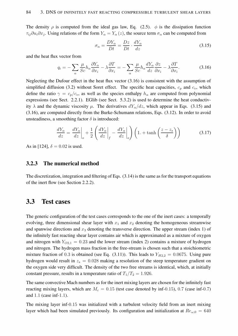
84 3. DNS OF INFINITELY FAST REACTING COMPRESSIBLE TURBULENT SHEAR LAYERS
The density ρ is computed from the ideal gas law, Eq. (2.5). φ is the dissipation functionτij∂ui∂xj . Using relations of the form Yα = Yα (z), the source term σα can be computed from
σα =DYαDt
=Dz
Dt· dYαdz
(3.15)
and the heat flux vector from
qi = −∑
α
µ
Schα∂Yα∂xi− λ∂T
∂xi= −
∑
α
µ
SchαdYαdz
∂z
∂xi− λ∂T
∂xi. (3.16)
Neglecting the Dufour effect in the heat flux vector (3.16) is consistent with the assumption ofsimplified diffusion (3.2) without Soret effect. The specific heat capacities, cp and cv, whichdefine the ratio γ = cp/cv, as well as the species enthalpy hα are computed from polynomialexpressions (see Sect. 2.2.1). EGlib (see Sect. 5.3.2) is used to determine the heat conductiv-ity λ and the dynamic viscosity µ. The derivatives dYα/dz, which appear in Eqs. (3.15) and(3.16), are computed directly from the Burke-Schumann relations, Eqs. (3.12). In order to avoidunsteadiness, a smoothing factor δ is introduced:
dYαdz
=dYαdz
∣∣∣∣o
+1
2
(dYαdz
∣∣∣∣f
− dYαdz
∣∣∣∣o
)(1.+ tanh
(z − zsδ
))(3.17)
As in [124], δ = 0.02 is used.
3.2.3 The numerical method
The discretization, integration and filtering of Eqs. (3.14) is the same as for the transport equationsof the inert flow (see Section 2.2.2).
3.3 Test cases
The generic configuration of the test cases corresponds to the one of the inert cases: a temporallyevolving, three dimensional shear layer with x1 and x2 denoting the homogeneous streamwiseand spanwise directions and x3 denoting the transverse direction. The upper stream (index 1) ofthe infinitely fast reacting shear layer contains air which is approximated as a mixture of oxygenand nitrogen with YO2,1 = 0.23 and the lower stream (index 2) contains a mixture of hydrogenand nitrogen. The hydrogen mass fraction in the free-stream is chosen such that a stoichiometricmixture fraction of 0.3 is obtained (see Eq. (3.11)). This leads to YH2,2 = 0.0675. Using purehydrogen would result in zs = 0.028 making a resolution of the steep temperature gradient onthe oxygen side very difficult. The density of the two free streams is identical, which, at initiallyconstant pressure, results in a temperature ratio of T1/T2 = 1.926.
The same convective Mach numbers as for the inert mixing layers are chosen for the infinitely fastreacting mixing layers, which are Mc = 0.15 (test case denoted by inf-0.15), 0.7 (case inf-0.7)and 1.1 (case inf-1.1).
The mixing layer inf-0.15 was initialized with a turbulent velocity field from an inert mixinglayer which had been simulated previously. Its configuration and initialization at Reω,0 = 640

TEST CASES 85
corresponds to case inert-0.15, except for the lengths of the domain (L1, L2 and L3) which aresmaller by a factor 1.5 for L1 and L2 and by a factor 2.25 for L3. The grid point numbers (N1, N2
and N3) in this pre-simulation were reduced by the same factors to keep the same resolution asin case inert-0.15. The inert mixing layer was computed until the Reynolds number reached thevalue Reω = 2300. Then, the velocity fields were scaled to match the free-stream velocities anddomain lengths of case inf-0.15 with a Reynolds number of Reω = 9200. Mac was kept constantduring this scaling. The increase in Reynolds number was necessary to reach a fully turbulentself-similar state with reasonable computational effort inspite of the laminarizing effect of heatrelease. The mixture fraction profile at initialization is a hyperbolic tangent with a vorticitythickness corresponding to Reω = 9200. The pressure is set constant, and the temperature isinitialized by the Burke-Schumann relation
T (z) =
{zTF,f + (1− z)TO,o +
Q0YF,fcp
z , if z < zs
zTF,f + (1− z)TO,o +Q0YF,fcp
zs1−z1−zs , if z ≥ zs
(3.18)
with the heat release Q0 =∑
α ναWα∆h0α/ (WFνF ), wherein ∆h0
α is the standard enthalpy offormation of species α at T 0 = 298K. This results in a peak temperature of 2642K at z = zs.Equation (3.18) is obtained with equal cp and diffusion coefficients D for all species and a Lewisnumber Le = λ/ (ρDcp) = 1. However, this linear relation is only used for initialization. Duringthe DNS, a transport equation for the temperature is integrated without the assumption of Le = 1
being used (cf. Eqs. (3.14)).
The initialization fields for case inf-0.7 were taken from inf-0.15 at Reω = 10000. They arescaled in a way that increases the convective Mach number to Mc = 0.7. Correspondingly, theinitialization of case inf-1.1 was done with fields from case inf-0.7 at Reω = 12800.
Grid and domain sizes of the infinitely fast reacting test cases are given in Table 3.1 and are thesame for all reacting test cases. The grid-spacing is constant in all directions.
To compare the infinitely fast reacting mixing layers with results in the literature, a non-dimensionalheat release term
Q =q0YF,fzs
c0p,N2T
0νFWF(3.19)
is computed. The enthalpy of reaction is given by [187]
q0 =∑
α
ναWα∆h0α. (3.20)
With the stoichiometric coefficients of reaction used in this study, νH2 = νF = 2, νO2 = 1 andνH2O = −2, as well as ∆h0
H20 = 13.425MJ/kg and ∆h0H2 = ∆h0
O2 = 0J/kg, an enthalpy ofreaction q0 = 483.693MJ/mol is obtained. Together with the specific heat of nitrogen at T 0,
Table 3.1: Geometrical parameters of the simulations inf-0.15, inf-0.7, inf-1.1. The computationaldomain has the dimensions L1, L2 and L3 with N1, N2 and N3 grid points, respectively. Thereference vorticity thickness δω,0 is chosen such that it results in Reω,0 = 640.
L1/δω,0 L2/δω,0 L3/δω,0 N1 N2 N3
345 86 172 768 192 432

86 3. DNS OF INFINITELY FAST REACTING COMPRESSIBLE TURBULENT SHEAR LAYERS
c0p,N2 = 1.038kJ/ (kgK), this results in Q = 7.856 which is close to the value that Pantano et
al. [124] had in their mixing layer simulation with the highest heat release rate (Q = 7.46 forhydrocarbon combustion).
3.4 Results and analysis
3.4.1 The structure of the infinitely fast reacting shear layers
In this section, instantaneous images of scalar (mixture fraction) fields of the infinitely fast react-ing mixing layers are shown in order to visualize changes that occur when their convective Machnumber is increased. Furthermore, comparisons of the figures with those of the inert mixinglayers in Sect. 2.4.1 are indicative of some consequences of heat release. Since the differencesbetween the infinitely fast reacting mixing layers are less pronounced than for inert mixing layersand since the characteristic features can already be seen from x1-x3-cuts, only such figures areshown in the following. For clarity, the analysis is limited to the self-similar state.
3.4.1.1 Infinitely fast reacting shear layer at Mc = 0.15
Figure 3.3 shows the instantaneous mixture fraction field of the mixing layer inf-0.15 at τω = 573
together with the stoichiometric isoline zs = 0.3 and the isolines, z = 0.1 and z = 0.9, formingthe turbulent boundary of the mixing layer (cf. Sect. 3.4.4.4). The temperature field is shown inFig. 3.4 at the same instant. At first sight, when comparing the figures with those in Chapter 2,the consequences of heat release seem to be similar to those of compressibility: A smootheningof the mixing layer as well as an increase of the dominant length scales, both within the mixinglayer and at its boundaries are visible. Less contorted fields involving heat release were alsoobserved by McMurtry et al. [109]. One obvious reason for this is the laminarizing effect of hightemperatures. In Fig. 3.4 no clear distinction between braids and rollers can be made which isin agreement with the observations of Hermanson & Dimotakis [72] who found heat release torender the boundaries between two merging structures invisible.
Figure 3.3: Case inf-0.15: Instantaneous mix-ture fraction field, x1-x3-plane in the middleof the computational domain at τω = 573, iso-lines z = 0.1, zs = 0.3 and z = 0.9 are shown
Figure 3.4: Case inf-0.15: Instantaneous tem-perature field, x1-x3-plane in the middle of thecomputational domain at τω = 573, isolinesz = 0.1, zs = 0.3 and z = 0.9 are shown

RESULTS AND ANALYSIS 87
Figure 3.5: Case inf-0.7: Instantaneous mix-ture fraction field, x1-x3-plane in the middleof the computational domain at τω = 761, iso-lines z = 0.1, zs = 0.3 and z = 0.9 are shown
Figure 3.6: Case inf-0.7: Instantaneous tem-perature field, x1-x3-plane in the middle of thecomputational domain at τω = 761, isolinesz = 0.1, zs = 0.3 and z = 0.9 are shown
Figure 3.7: Case inf-1.1: Instantaneous mix-ture fraction field, x1-x3-plane in the middleof the computational domain at τω = 803, iso-lines z = 0.1, zs = 0.3 and z = 0.9 are shown
Figure 3.8: Case inf-1.1: Instantaneous tem-perature field, x1-x3-plane in the middle of thecomputational domain at τω = 803, isolinesz = 0.1, zs = 0.3 and z = 0.9 are shown
3.4.1.2 Infinitely fast reacting shear layers at Mc = 0.7 and Mc = 1.1
At higher convective Mach numbers, the mixing layers become even less corrugated with thedominant length scales increasing further (cf. Figs. 3.5 to 3.8), which is in agreement withPlanche & Reynolds [141]. A little increase of the maximum temperature compared to Fig. 3.4(cf. respective scales) due to additional heating by dissipation can be noted. The ondulations ofthe isolines have a smaller vertical extent than for the incompressible reacting mixing layer whichpoints towards a reduction of intermittency.
3.4.2 The self-similar state
As for the inert mixing layers, the infinitely fast reacting mixing layers reach self-similar stateswith constant momentum thickness growth rates as shown by Fig. 3.9. With increasing com-pressibility, the growth rates reduce. The same is true for the product mass thicknesses [72]
δP =
∫ ∞
−∞
〈ρ〉〈YP 〉fρ0YP (zs)
dx3 (3.21)
in Fig. 3.10.
Table 3.2 gives the non-dimensional times for the beginning and the end of the self-similar statesalong with the corresponding Reynolds numbers. The higher the convective Mach number, thelonger it takes to reach the self-similar state which is due to the stabilizing effect of compressibil-ity. The same has already been observed for the inert test cases. The Reynolds numbers Reω arehigher during the self-similar state of the reacting mixing layers than the ones of the inert mixinglayers (cf. Table 2.2) which is due to the fact that the initial Reynolds numbers of the reacting

88 3. DNS OF INFINITELY FAST REACTING COMPRESSIBLE TURBULENT SHEAR LAYERS
τω
δ θ/δθ,0
2000150010005000
8
7
6
5
43
2
1
0
Figure 3.9: Temporal development of the momentum thickness, normalized by the initial mo-mentum thickness δθ,0, ∗: inf-0.15, �: inf-0.7, ◦: inf-1.1, dashed lines show linear regressionsfor the self-similar state
τω
δ P/δP,0
2000150010005000
8
7
6
5
43
2
1
0
Figure 3.10: Temporal development of the product mass thickness, normalized by the initialproduct mass thickness δθ,0, symbols as in Fig. 3.9, dashed lines show linear regressions for theself-similar statemixing layers have been increased (see Sect. 3.3). However, since the Reynolds numbers duringthe self-similar state of all simulations differ by less than a factor of 3 and are therefore within thesame order of magnitude, it is reasonable to attribute different behaviours to compressibility andheat release rather than to different Reynolds numbers. The peak micro-scale Reynolds numbersgiven in Table 3.2 are significantly smaller than the ones in Table 2.2 which is due to the increaseof viscosity in the reacting mixing layers. This is in agreement with the laminarizing effect ofheat release noticed already in Sect. 3.4.1.
The non-dimensional momentum thickness growth rates δθ (according to Eq. (2.19)) are 0.0042
for case inf-0.15, 0.0037 for case inf-0.7 and 0.0030 for case inf-1.1. All these values are signifi-cantly smaller than the ones for the inert mixing layers at the respective Reynolds numbers, which
Table 3.2: Dimensionless times and Reynolds numbers at the beginning (index: B) and end (in-dex: E) of the self-similar state
τω,B τω,E Reω,B Reω,E Reλ,B Reλ,E
inf-0.15 459 803 23810 32450 37 41inf-0.7 761 1216 22150 33970 34 40inf-1.1 803 2047 20750 37780 36 46

RESULTS AND ANALYSIS 89
x3/δω
〈z′′ z′′ 〉f
10.50-0.5-1
0.07
0.06
0.05
0.04
0.03
0.02
0.01
0
Figure 3.11: Case inf-0.15: Spatially averagedprofiles of the mixture fraction variance 〈z ′′z′′〉fat different times, +: τω = 124, ×: τω = 234,∗: τω = 346, �: τω = 459, �: τω = 573, ◦:τω = 688, •: τω = 803
x3/δω
〈z′′ z′′ 〉f
10.50-0.5-1
0.045
0.04
0.035
0.03
0.025
0.02
0.015
0.01
0.005
0
Figure 3.12: Case inf-0.7: Spatially averagedprofiles of the mixture fraction variance 〈z ′′z′′〉fat different times, +: τω = 344, ×: τω = 485,∗: τω = 625, �: τω = 761, �: τω = 897, ◦:τω = 1034, •: τω = 1170
x3/δω
〈z′′ z′′ 〉f
10.50-0.5-1
0.045
0.04
0.035
0.03
0.025
0.02
0.015
0.01
0.005
0
Figure 3.13: Case inf-1.1: Spatially averagedprofiles of the mixture fraction variance 〈z ′′z′′〉fat different times, +: τω = 305, ×: τω = 665,∗: τω = 999, �: τω = 1195, �: τω = 1388, ◦:τω = 1582, •: τω = 1779
is in agreement with the results of other authors [72, 109]. The effect of compressibility is not aspronounced for the reacting cases as for the inert ones and consists in a decrease by just a factorof 1.4 between the growth rates of the lowest and the highest Mc (factor 3.4 for the inert cases).Taking into account molecular dissipation effects when computing δθ (cf. Eq. (2.18)) results indifferences of less than 4 % compared with the previously given values. Therefore, such effectscan be neglected and the use of Eq. (2.19) is justified.
The relaxation towards self-similar states is not only checked by verifying whether the growthrates are approximately constant, but also by examining the normalized spatially averaged profilesof important flow quantities as e.g. the mixture fraction variance 〈z ′′z′′〉f in Figs. 3.11 to 3.13.The collapse of the profiles onto one ’single’ curve during the self-similar state is clearly visible.Therefore, all profiles presented in the following are not only averaged over the two homogeneousdirections but also temporally over the self-similar states (if not specified otherwise).
3.4.3 Check of resolution and domain sizes
All simulations are well resolved with a local minimum of the Kolmogorov length lk (Eq. (2.34))of 0.77∆x3 for case inf-0.15, 0.78∆x3 for case inf-0.7 and 0.9∆x3 for case inf-1.1 during the self-similar state. In contrast to the inert flows where the minimal Kolmogorov lengths are found inthe center of the shear layers, the minimal Kolmogorov lengths in the reacting cases are situatedat the edges of the layers and the corresponding profiles present a peak close to the center of

90 3. DNS OF INFINITELY FAST REACTING COMPRESSIBLE TURBULENT SHEAR LAYERS
∆x1/L1
R1u
1
0.50.450.40.350.30.250.20.150.10.050
1
0.8
0.6
0.4
0.2
0
-0.2
Figure 3.14: Two-point correlation R1 withf = u1, in the middle of the computational do-main, averaged over the self-similar state, ∗:inf-0.15, �: inf-0.7, ◦: inf-1.1
∆x2/L2
R2u
1
0.50.450.40.350.30.250.20.150.10.050
1
0.8
0.6
0.4
0.2
0
-0.2
Figure 3.15: Two-point correlation R2 withf = u1, in the middle of the computationaldomain, averaged over the self-similar state,symbols as in Fig. 3.14
∆x1/L1
R1u
3
0.50.450.40.350.30.250.20.150.10.050
1
0.8
0.6
0.4
0.2
0
-0.2
Figure 3.16: Two-point correlation R1 withf = u3, in the middle of the computationaldomain, averaged over the self-similar state,symbols as in Fig. 3.14
∆x2/L2
R2u
30.50.450.40.350.30.250.20.150.10.050
1
0.8
0.6
0.4
0.2
0
-0.2
Figure 3.17: Two-point correlation R2 withf = u3, in the middle of the computationaldomain, averaged over the self-similar state,symbols as in Fig. 3.14
∆x1/L1
R1z
0.50.450.40.350.30.250.20.150.10.050
1
0.8
0.6
0.4
0.2
0
-0.2
Figure 3.18: Two-point correlation R1 withf = z, in the middle of the computationaldomain, averaged over the self-similar state,symbols as in Fig. 3.14
∆x2/L2
R2z
0.50.450.40.350.30.250.20.150.10.050
1
0.8
0.6
0.4
0.2
0
-0.2
Figure 3.19: Two-point correlation R2 withf = z, in the middle of the computationaldomain, averaged over the self-similar state,symbols as in Fig. 3.14
the shear layers. This is due to the increased viscosity at the center that goes along with thetemperature peak at the location of the flame.
Since a Schmidt number of Sc = 0.7 < 1 is used for the mixture fraction and all species, noresolution problems concerning the scalar fields are expected. Spectra that also demonstrate theappropriateness of the resolution and, therefore, show no spurious accumulation of energy in thehighest wavenumbers are shown in Sects. 3.4.4.2 and 3.4.4.3.
The domain sizes of the simulations in the periodic directions are large enough which is shownby the two-point correlations of the velocity components and the mixture fraction (Figs. 3.14 to3.19), computed according to Eqs. (2.35) and (2.36). The two-point correlations are small in themiddle of the domain.
The integral length scales, Eqs. (2.37) and (2.38), which are given in Table 3.3, are small com-

RESULTS AND ANALYSIS 91
Table 3.3: Integral length scales
l1/L1 l2/L2
inf-0.15 0.067 0.041inf-0.7 0.098 0.041inf-1.1 0.094 0.035
pared to the dimensions of the computational box which confirms the appropriateness of its size.
3.4.4 Effects of compressibility and heat release
3.4.4.1 Mean heat release term
Figure 3.20 shows the term in the pressure equation that describes the heat release effect,
Qp = − (γ − 1) ρ∑
α
hασα (3.22)
with σα computed according to Eq. (3.15). The reduction of its peak value with compressibility isstriking, and the term becomes nearly negligible at Mc = 1.1. The peak value of the heat releaseterm is situated to the right of the mixing layer center, which is the side where the stoichiometricsurface is located.
The conclusion which can be drawn from Fig. 3.20 and which is confirmed by many of the resultsin the subsequent sections is that heat release due to infinitely fast chemical reactions has a muchlarger influence on the mixing layer with Mc = 0.15 than on the ones with higher Mc where thedifferences between the statistics for the inert and reacting mixing layers are small.
3.4.4.2 Turbulence characteristics
Mean flow variables The mean temperature in Fig. 3.21 and the mean density in Fig. 3.22show the influence of heat release which leads to a temperature maximum and a density minimum.
x3/δω
Qpδ ω/
[(γ−
1)∆u
3ρ
0]
10.50-0.5-1
21.81.61.41.2
10.80.60.40.2
0-0.2
Figure 3.20: Averaged heat release termQ = Qp/ (γ − 1), normalized by ρ0∆u3/δω, ∗: inf-0.15,�: inf-0.7, ◦: inf-1.1

92 3. DNS OF INFINITELY FAST REACTING COMPRESSIBLE TURBULENT SHEAR LAYERS
The location of these extrema is not in the center of the shear layer, but shifted to the oxygen-rich side of the layer since the stoichiometric mixture fraction is zs = 0.3. The influence ofcompressibility on the peak value of the temperature is less pronounced for the infinitely fastreacting mixing layers than for the inert ones (cf. Sect. 2.4.4.1): The peak value is only slightlyincreasing with Mc due to dissipative heating. A larger difference between case inf-0.15 and theother two reacting cases at higherMc concerns the widths of the temperature and density profiles:The profiles at Mc = 0.15 are broader than the others leading to smaller gradients.
As for the inert mixing layers, the averaged pressure of the reacting cases, shown in Fig. 3.23,drops with γM 2
c and is nearly constant across the layer in each test case, respectively, which leadsto the conclusion that temperature and density are mutually dependent.
The influence of compressibility on the Favre averaged velocity profiles in Fig. 3.24 is small.However, there is a difference between the Favre averaged profiles with and without heat releaseas shown in Fig. 3.25 for the cases withMc = 0.7: On the fuel side, the profile with heat release isabove the profile without heat release with the latter being very similar to the Reynolds averagedprofile with heat release. On the oxygen side, the Favre averaged profile with heat release isbelow the Favre averaged profile without heat release and below the Reynolds averaged profilewith heat release. Since the relation
〈u1〉f − 〈u1〉 =〈ρ′u′1〉〈ρ〉 (3.23)
holds, it can be concluded that the correlation between ρ′ and u′1 is positive on the fuel side andnegative on the oxygen side of the reacting mixing layer. This is understandable since highervelocity, i.e. positive u′1, is related with colder fluid (positive ρ′) on the fuel side and hotter fluid(negative ρ′) on the oxygen side.
x3/δω
〈T〉/T
0
10.50-0.5-1
4.5
4
3.5
3
2.5
2
1.5
1
0.5
Figure 3.21: Averaged temperature, normal-ized by T0 = 0.5 (T1 + T2), ∗: inf-0.15, �:inf-0.7, ◦: inf-1.1
x3/δω
〈ρ〉/ρ
0
10.50-0.5-1
1.1
1
0.9
0.8
0.7
0.6
0.5
0.4
0.3
0.2
Figure 3.22: Averaged density, normalized byρ0, symbols as in Fig. 3.21
x3/δω
〈p〉/
(ρ0∆u
2)
10.50-0.5-1
9
8
7
6
5
4
3
2
1
0
Figure 3.23: Averaged pressure, normalizedby ρ0∆u2, symbols as in Fig. 3.21
x3/δω
〈u〉 f/∆
u
10.50-0.5-1
0.50.40.30.20.1
0-0.1-0.2-0.3-0.4-0.5
Figure 3.24: Favre averaged streamwise veloc-ity, normalized by ∆u, symbols as in Fig. 3.21

RESULTS AND ANALYSIS 93
x3/δω10.50-0.5-1
0.50.40.30.20.1
0-0.1-0.2-0.3-0.4-0.5
Figure 3.25: Mass-weighted and Reynolds averaged streamwise velocities, cases with Mc = 0.7,solid: 〈u〉f/∆u of case inf-0.7, dashed: 〈u〉/∆u of case inf-0.7, dotted: 〈u〉/∆u of case inert-0.7
Reynolds stresses, turbulent kinetic energy and anisotropies Figures 3.26 to 3.30 show thecomponents of the Reynolds stress tensor and the TKE. As for the inert test cases (cf. Figs.2.67 to 2.71), the peak values are decreasing with increasing compressibility. However, for thereacting mixing layers the reduction is not as strong as for the inert ones. The higher Mc thesmaller the differences between the profiles with and without heat release. This is in agreementwith the behaviour of the normalized heat release term which becomes negligible at high Mc (cf.Sect. 3.4.4.1). Particularly striking is the reduction of the magnitude of the low Mc profiles withreaction and heat release with respect to the ones without: reductions of about 69 % for the peakvalues of the Reynolds shear stresses and of about 60 % for the peak value of the TKE for thetest cases at Mc = 0.15, respectively are observed. The reduction of the Reynolds shear stress isconsistent with the reduction of the momentum thickness growth rate by 66 % (from 0.0124 forcase inert-0.15 to 0.0042 for case inf-0.15) caused by heat release, since the latter directly dependson 〈ρ〉R13/ρ0 (cf. Eq. (2.19)). A reduction of the Reynolds shear stress by heat release also means
x3/δω
〈ρ〉R
11/
(ρ0∆u
2)
10.50-0.5-1
0.010.0090.0080.0070.0060.0050.0040.0030.0020.001
0
Figure 3.26: Streamwise Reynolds stress〈ρ〉R11, normalized by ρ0∆u2, curves as inFig. 3.21
x3/δω
〈ρ〉R
22/
(ρ0∆u
2)
10.50-0.5-1
0.006
0.005
0.004
0.003
0.002
0.001
0
Figure 3.27: Spanwise Reynolds stress 〈ρ〉R22,normalized by ρ0∆u2, curves as in Fig. 3.21
x3/δω
〈ρ〉R
33/
(ρ0∆u
2)
10.50-0.5-1
0.0045
0.004
0.0035
0.003
0.0025
0.002
0.0015
0.001
0.0005
0
Figure 3.28: Reynolds stress 〈ρ〉R33, normal-ized by ρ0∆u2, curves as in Fig. 3.21
x3/δω
〈ρ〉R
13/
(ρ0∆u
2)
10.50-0.5-1
0
-0.0005
-0.001
-0.0015
-0.002
-0.0025
-0.003
Figure 3.29: Reynolds stress 〈ρ〉R13, normal-ized by ρ0∆u2, curves as in Fig. 3.21
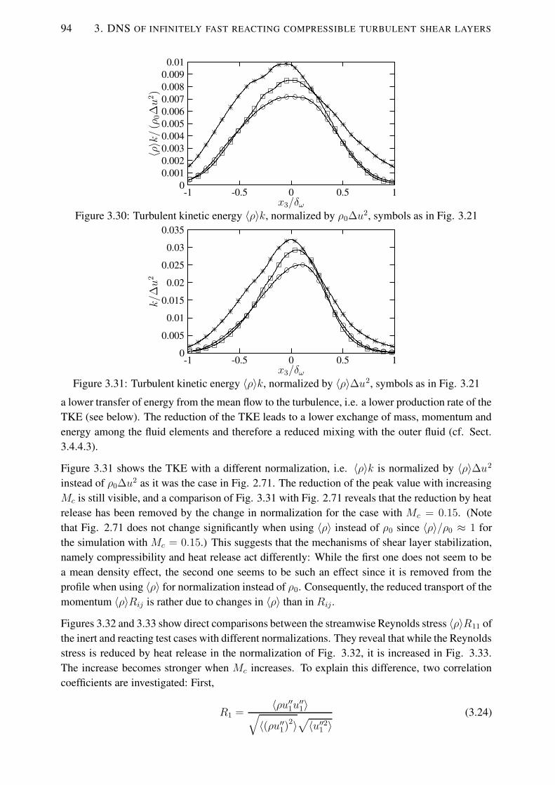
94 3. DNS OF INFINITELY FAST REACTING COMPRESSIBLE TURBULENT SHEAR LAYERS
x3/δω
〈ρ〉k/
(ρ0∆u
2)
10.50-0.5-1
0.010.0090.0080.0070.0060.0050.0040.0030.0020.001
0
Figure 3.30: Turbulent kinetic energy 〈ρ〉k, normalized by ρ0∆u2, symbols as in Fig. 3.21
x3/δω
k/∆
u2
10.50-0.5-1
0.035
0.03
0.025
0.02
0.015
0.01
0.005
0
Figure 3.31: Turbulent kinetic energy 〈ρ〉k, normalized by 〈ρ〉∆u2, symbols as in Fig. 3.21
a lower transfer of energy from the mean flow to the turbulence, i.e. a lower production rate of theTKE (see below). The reduction of the TKE leads to a lower exchange of mass, momentum andenergy among the fluid elements and therefore a reduced mixing with the outer fluid (cf. Sect.3.4.4.3).
Figure 3.31 shows the TKE with a different normalization, i.e. 〈ρ〉k is normalized by 〈ρ〉∆u2
instead of ρ0∆u2 as it was the case in Fig. 2.71. The reduction of the peak value with increasingMc is still visible, and a comparison of Fig. 3.31 with Fig. 2.71 reveals that the reduction by heatrelease has been removed by the change in normalization for the case with Mc = 0.15. (Notethat Fig. 2.71 does not change significantly when using 〈ρ〉 instead of ρ0 since 〈ρ〉/ρ0 ≈ 1 forthe simulation with Mc = 0.15.) This suggests that the mechanisms of shear layer stabilization,namely compressibility and heat release act differently: While the first one does not seem to bea mean density effect, the second one seems to be such an effect since it is removed from theprofile when using 〈ρ〉 for normalization instead of ρ0. Consequently, the reduced transport of themomentum 〈ρ〉Rij is rather due to changes in 〈ρ〉 than in Rij .
Figures 3.32 and 3.33 show direct comparisons between the streamwise Reynolds stress 〈ρ〉R11 ofthe inert and reacting test cases with different normalizations. They reveal that while the Reynoldsstress is reduced by heat release in the normalization of Fig. 3.32, it is increased in Fig. 3.33.The increase becomes stronger when Mc increases. To explain this difference, two correlationcoefficients are investigated: First,
R1 =〈ρu′′1u′′1〉√
〈(ρu′′1)2〉√〈u′′21 〉
(3.24)

RESULTS AND ANALYSIS 95
x3/δω
〈ρ〉R
11/
(ρ0∆u
2)
10.50-0.5-1
0.03
0.025
0.02
0.015
0.01
0.005
0
Figure 3.32: Reynolds stress 〈ρ〉R11, normalized by ρ0∆u2, solid: reacting cases, dashed: inertcases, ∗: Mc = 0.15, �: Mc = 0.7, ◦: Mc = 1.1
x3/δω
R11/∆
u2
10.50-0.5-1
0.035
0.03
0.025
0.02
0.015
0.01
0.005
0
Figure 3.33: Reynolds stress 〈ρ〉R11, normalized by 〈ρ〉∆u2, lines and symbols as in Fig. 3.32
which is the correlation coefficient between the mass flux ρu′′1 and the velocity fluctuation u′′1.Second, the correlation coefficient
R2 =〈u′′1u′′1〉f〈u′′21 〉
. (3.25)
R1, which is shown in Fig. 3.34 for the various mixing layers, is indicative of the behaviourof 〈ρ〉R11 in the normalization of Fig. 3.32, i.e. 〈ρ〉R11/ (ρ0∆u2) = 〈ρu′′1u′′1〉/ (ρ0∆u2): Bothdecrease when heat release sets in. This means that the decrease of 〈ρu′′1u′′1〉/ (ρ0∆u2) is due to adecrease in the correlation between ρu′′1 and u′′1. Ratio R2 in Fig. 3.35, on the contrary, increasesin the center of the shear layer for the reacting test cases. The difference between the curves ofR2 for two corresponding (inert and reacting) test cases at the same Mc increases with increasingMc. The same features can be noticed in Fig. 3.33, which confirms that R2 is indicative of thebehaviour of 〈R11〉/∆u2 = 〈u′′1u′′1〉f/∆u2.
The reductions of the Reynolds stresses and the TKE by heat release in the normalization ofFigs. 3.26 to 3.30 compared to Figs. 2.67 to 2.71 are in agreement with the results of otherauthors [109, 115, 124]. McMurtry et al. [109] found a decrease of the profiles 〈ρ〉R13 and 〈ρ〉k.Using their density decrease of about 〈ρ〉/ρ0 = 0.5 and dividing the magnitude of the peak valuesof 〈ρ〉k (from Fig. 12 in [109]) by this ratio, results in peak values for ρ0k and therefore alsofor k/∆u2 that are nearly constant despite heat release. This is in agreement with the presentfindings (Fig. 2.71). Moreover, Hermanson & Demotakis [72] showed by an analysis that thedensity changes alone suffice to reduce the Reynolds shear stress consistently with the observeddecrease in shear layer growth rate.

96 3. DNS OF INFINITELY FAST REACTING COMPRESSIBLE TURBULENT SHEAR LAYERS
x3/δω
R1
10.50-0.5-1
1.2
1.1
1
0.9
0.8
0.7
0.6
0.5
Figure 3.34: Correlation coefficient R1 = 〈ρu′′1u′′1〉/(√〈(ρu′′1)2〉
√〈u′′21 〉
), lines and symbols as
in Fig. 3.32
x3/δω
R2
10.50-0.5-1
1.2
1.1
1
0.9
0.8
0.7
0.6
0.5
Figure 3.35: Correlation coefficient R2 = 〈u′′1u′′1〉f/〈u′′21 〉, lines and symbols as in Fig. 3.32
In contrast to this and also to the present results, Pantano et al. [124] noted a reduction of theTKE by heat release by about 30 % when using the normalization of Fig. 3.31. However, whenincreasing the heat release to the highest level with which these authors perform a DNS, thecorresponding figure in [124] shows once again an increase in the TKE which the authors do notcomment on, but which is in agreement with the present results. Two other features that can beseen in Fig. 3.31, namely the pointed shape and the shift of the peak value to the side of the shearlayer where the stoichiometric surface is located are also in agreement with what Pantano et al.observe.
What the anisotropy of the Reynolds stresses is concerned, the present results reveal that there isnot much influence due to heat release. Plotting the anisotropy parameters from Eqs. (2.39) and(2.40) would result in figures (not shown) that are very similar to the ones presented for the inertmixing layers, i.e. Figs. (2.72) to (2.75). The conclusion that compressibility has little effect onthe anisotropy of the Reynolds stresses in the full turbulent, self-similar state and in the Machnumber range considered applies therefore also to the present shear layers with heat release.
Reynolds stress transport equations Figures 3.36 to 3.43 show the major terms in the Reynoldsstress transport equations (2.28) for the reacting mixing layers. All comments made about the re-spective role of these terms in Sect. 2.4.4.1 also apply here, one example being the redistributiveaction of the pressure-strain terms on the fluctuating energy from the streamwise component ofthe Reynolds stresses to the spanwise and transverse components. Comparing the figures with the

RESULTS AND ANALYSIS 97
x3/δω10.50-0.5-1
0.006
0.005
0.004
0.003
0.002
0.001
0
-0.001
-0.002
Figure 3.36: Budget of R11, normalized by ρ0∆u3/δω, symbols as in Fig. 3.21, solid: production,dashed: dissipation rate
x3/δω10.50-0.5-1
0.001
0.0005
0
-0.0005
-0.001
-0.0015
-0.002
-0.0025
-0.003
Figure 3.37: Budget of R11, normalized by ρ0∆u3/δω, symbols as in Fig. 3.21, solid: pressure-strain rate, dashed: turbulent transport
corresponding ones for the inert mixing layers (Figs. 2.76 to 2.83), a reduction of all non-zeroterms due to heat release is obvious. It is between 60 % and 70 % for Mc = 0.15 which is com-parable to the reduction of other quantities (momentum thickness growth rate, Reynolds stresses,TKE) that have been investigated previously. The reduction is less for higher Mc since the influ-ence of compressibility on the budget terms is less pronounced for the reacting shear layers thanfor the inert ones; so, heat release has a larger influence at low Mc.
The relatively weak reduction of the production terms, pressure-strain correlations and dissipation
x3/δω10.50-0.5-1
0.0002
0
-0.0002
-0.0004
-0.0006
-0.0008
-0.001
-0.0012
-0.0014
Figure 3.38: Budget of R22, normalized by ρ0∆u3/δω, symbols as in Fig. 3.21, solid: production,dashed: dissipation rate
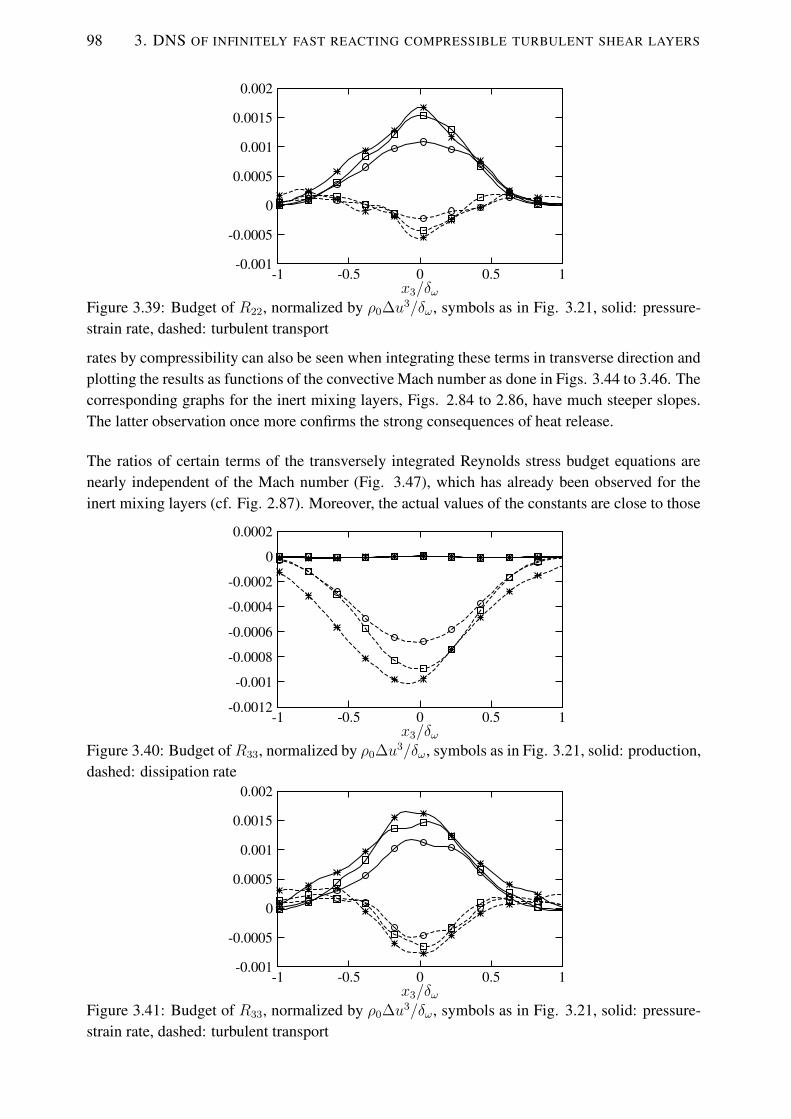
98 3. DNS OF INFINITELY FAST REACTING COMPRESSIBLE TURBULENT SHEAR LAYERS
x3/δω10.50-0.5-1
0.002
0.0015
0.001
0.0005
0
-0.0005
-0.001
Figure 3.39: Budget of R22, normalized by ρ0∆u3/δω, symbols as in Fig. 3.21, solid: pressure-strain rate, dashed: turbulent transport
rates by compressibility can also be seen when integrating these terms in transverse direction andplotting the results as functions of the convective Mach number as done in Figs. 3.44 to 3.46. Thecorresponding graphs for the inert mixing layers, Figs. 2.84 to 2.86, have much steeper slopes.The latter observation once more confirms the strong consequences of heat release.
The ratios of certain terms of the transversely integrated Reynolds stress budget equations arenearly independent of the Mach number (Fig. 3.47), which has already been observed for theinert mixing layers (cf. Fig. 2.87). Moreover, the actual values of the constants are close to those
x3/δω10.50-0.5-1
0.0002
0
-0.0002
-0.0004
-0.0006
-0.0008
-0.001
-0.0012
Figure 3.40: Budget of R33, normalized by ρ0∆u3/δω, symbols as in Fig. 3.21, solid: production,dashed: dissipation rate
x3/δω10.50-0.5-1
0.002
0.0015
0.001
0.0005
0
-0.0005
-0.001
Figure 3.41: Budget of R33, normalized by ρ0∆u3/δω, symbols as in Fig. 3.21, solid: pressure-strain rate, dashed: turbulent transport

RESULTS AND ANALYSIS 99
x3/δω10.50-0.5-1
0.00050
-0.0005-0.001
-0.0015-0.002
-0.0025-0.003
-0.0035-0.004
-0.0045
Figure 3.42: Budget of R13, normalized by ρ0∆u3/δω, symbols as in Fig. 3.21, solid: production,dashed: dissipation rate
x3/δω10.50-0.5-1
0.00350.003
0.00250.002
0.00150.001
0.00050
-0.0005-0.001
-0.0015
Figure 3.43: Budget of R13, normalized by ρ0∆u3/δω, symbols as in Fig. 3.21, solid: pressure-strain rate, dashed: turbulent transport
without heat release. Figure 3.47 shows that P13 ≈ 1.13Π11 and Π13 ≈ −0.96Π11. Neglectingε13 (|ε13| ≤ 0.05
∣∣∣P13
∣∣∣), the budget equation for R13 from Eqs. (2.43) can be simplified to
∂〈ρ〉R13
∂t= 1.13Π11 − 0.96Π11 = 0.17Π11. (3.26)
A very similar relation has been obtained for the inert mixing layers, ∂(〈ρ〉R13
)/∂t = 0.15Π11.
This suggests that the approximate relation (3.26) is not only valid for different Mc but also withand without heat release. As a consequence, the streamwise pressure-strain rate, Π11 is not onlyinfluencing R11 directly but also via its production rate P11 that is linked with R13 by Eq. (2.41).
Mc
∣ ∣ ∣Pij
∣ ∣ ∣/(ρ
0∆u
3)
1.21.110.90.80.70.60.50.40.30.20.1
0.00450.004
0.00350.003
0.00250.002
0.00150.001
0.00050
-0.0005
Figure 3.44: Production, integrated in trans-verse direction, normalized by ρ0∆u3: +: P11,◦: P22, ∗: P33, �: P13
Mc
∣ ∣ ∣Πij
∣ ∣ ∣/(ρ
0∆u
3)
1.21.110.90.80.70.60.50.40.30.20.1
0.0028
0.0026
0.0024
0.0022
0.002
0.0018
0.0016
0.0014
0.0012
0.001
Figure 3.45: Pressure-strain rate, integrated intransverse direction, normalized by ρ0∆u3: +:Π11, ◦: Π22, ∗: Π33, �: Π13
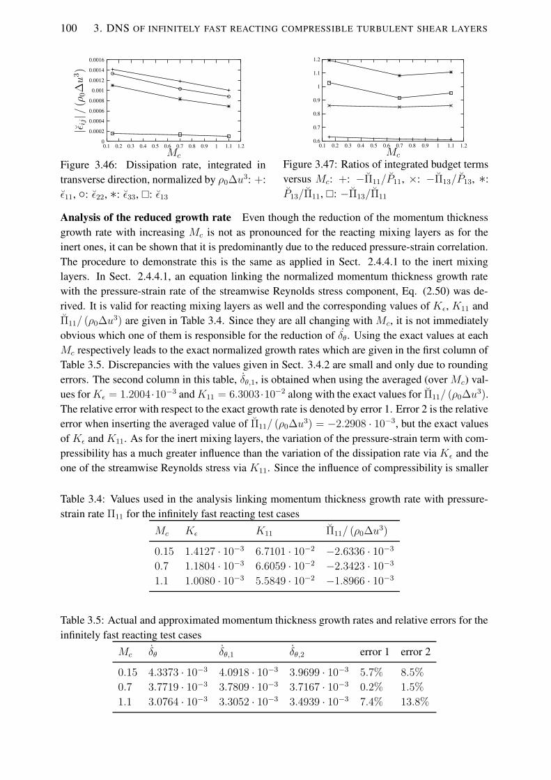
100 3. DNS OF INFINITELY FAST REACTING COMPRESSIBLE TURBULENT SHEAR LAYERS
Mc
|ε ij|/
(ρ0∆u
3)
1.21.110.90.80.70.60.50.40.30.20.1
0.0016
0.0014
0.0012
0.001
0.0008
0.0006
0.0004
0.0002
0
Figure 3.46: Dissipation rate, integrated intransverse direction, normalized by ρ0∆u3: +:ε11, ◦: ε22, ∗: ε33, �: ε13
Mc
1.21.110.90.80.70.60.50.40.30.20.1
1.2
1.1
1
0.9
0.8
0.7
0.6
Figure 3.47: Ratios of integrated budget termsversus Mc: +: −Π11/P11, ×: −Π13/P13, ∗:P13/Π11, �: −Π13/Π11
Analysis of the reduced growth rate Even though the reduction of the momentum thicknessgrowth rate with increasing Mc is not as pronounced for the reacting mixing layers as for theinert ones, it can be shown that it is predominantly due to the reduced pressure-strain correlation.The procedure to demonstrate this is the same as applied in Sect. 2.4.4.1 to the inert mixinglayers. In Sect. 2.4.4.1, an equation linking the normalized momentum thickness growth ratewith the pressure-strain rate of the streamwise Reynolds stress component, Eq. (2.50) was de-rived. It is valid for reacting mixing layers as well and the corresponding values of Kε, K11 andΠ11/ (ρ0∆u3) are given in Table 3.4. Since they are all changing with Mc, it is not immediatelyobvious which one of them is responsible for the reduction of δθ. Using the exact values at eachMc respectively leads to the exact normalized growth rates which are given in the first column ofTable 3.5. Discrepancies with the values given in Sect. 3.4.2 are small and only due to roundingerrors. The second column in this table, δθ,1, is obtained when using the averaged (over Mc) val-ues forKε = 1.2004·10−3 andK11 = 6.3003·10−2 along with the exact values for Π11/ (ρ0∆u3).The relative error with respect to the exact growth rate is denoted by error 1. Error 2 is the relativeerror when inserting the averaged value of Π11/ (ρ0∆u3) = −2.2908 · 10−3, but the exact valuesof Kε and K11. As for the inert mixing layers, the variation of the pressure-strain term with com-pressibility has a much greater influence than the variation of the dissipation rate via Kε and theone of the streamwise Reynolds stress via K11. Since the influence of compressibility is smaller
Table 3.4: Values used in the analysis linking momentum thickness growth rate with pressure-strain rate Π11 for the infinitely fast reacting test cases
Mc Kε K11 Π11/ (ρ0∆u3)
0.15 1.4127 · 10−3 6.7101 · 10−2 −2.6336 · 10−3
0.7 1.1804 · 10−3 6.6059 · 10−2 −2.3423 · 10−3
1.1 1.0080 · 10−3 5.5849 · 10−2 −1.8966 · 10−3
Table 3.5: Actual and approximated momentum thickness growth rates and relative errors for theinfinitely fast reacting test cases
Mc δθ δθ,1 δθ,2 error 1 error 2
0.15 4.3373 · 10−3 4.0918 · 10−3 3.9699 · 10−3 5.7% 8.5%
0.7 3.7719 · 10−3 3.7809 · 10−3 3.7167 · 10−3 0.2% 1.5%
1.1 3.0764 · 10−3 3.3052 · 10−3 3.4939 · 10−3 7.4% 13.8%

RESULTS AND ANALYSIS 101
Table 3.6: Averaged values (respective inert and reacting cases taken into account) used in theanalysis for each convective Mach number
Mc Kε K11 Π11/ (ρ0∆u3)
0.15 2.2486 · 10−3 8.6266 · 10−2 −5.5154 · 10−3
0.7 1.5100 · 10−3 6.4148 · 10−2 −2.8739 · 10−3
1.1 1.1455 · 10−3 4.7746 · 10−2 −2.1493 · 10−3
Table 3.7: Actual and approximated momentum thickness growth rates and relative errorsCase δθ δθ,3 δθ,4 error 3 error 4
inert-0.15 1.2835 · 10−2 1.1651 · 10−2 9.6134 · 10−2 9.2% 25.1%
inf-0.15 4.3373 · 10−3 5.3431 · 10−3 7.4264 · 10−3 23.2% 71.2%
inert-0.7 5.5930 · 10−3 5.2523 · 10−3 5.0262 · 10−3 6.1% 10.1%
inf-0.7 3.7719 · 10−3 4.1163 · 10−3 4.3410 · 10−3 9.1% 15.1%
inert-1.1 3.8371 · 10−3 3.7254 · 10−3 3.5740 · 10−3 2.9% 6.9%
inf-1.1 3.0764 · 10−3 3.2040 · 10−3 3.3441 · 10−3 4.1% 8.7%
for the reacting cases than for the inert ones, the errors in Table 3.5 are smaller than the ones inTable 2.5.
Similarly to the just described procedure, it can be shown that the pressure-strain correlations arealso the reason for the reduction in momentum growth rate with heat release. To do so, averagedvalues of Kε, K11 and Π11/ (ρ0∆u3) for each Mach number computed from the respective inertand reacting test cases are determined and given in Table 3.6. To evaluate δθ,3, the averaged valuesof Kε and K11 but the exact values of Π11/ (ρ0∆u3) (from Tables 2.4 and 3.4) are taken. For δθ,3,the averaged Π11/ (ρ0∆u3) are used along with the exact Kε and K11. The values for δθ,3 andδθ,4 are given in Table 3.7. Errors 3 and 4 are computed with respect to the exact growth rates δθwhich are repeated in the table for clarity. Since error 4 is in all cases larger than error 3, it is thepressure-strain correlation that has the largest influence on the growth rates and their reductionwith heat release. Since the influence of heat release is reduced with increasing Mc the errors atMc = 1.1 are considerably smaller than those at lower Mc.
Pressure-strain terms The pressure-strain term Π11 in the streamwise Reynolds stress trans-port equation has been shown in the last paragraph to be responsible for the reduction of thenormalized momentum thickness growth rate due to compressibility and heat release. Therefore,it is of interest to see what causes the reduction of Π11 = 2〈p′ ∂u′′1
∂x1〉. Figures 3.48 to 3.50 sug-
gest that the reduced pressure fluctuations, the rms value of which is shown in Fig. 3.48, arethe most probable cause for the reduction of the pressure-strain term Π11 with Mc, since the rmsvalue of ∂u′′1/∂x1 is only slightly influenced by compressibility and the correlation coefficientR (p, ∂u1/∂x1) oscillates around zero for all convective Mach numbers. Figure 3.51 even revealsthat the integrated value of the strain rate fluctuations rises slightly for an increase of Mc from 0.7
to 1.1.
When comparing the figures which contain the rms values of the pressure fluctuations and the

102 3. DNS OF INFINITELY FAST REACTING COMPRESSIBLE TURBULENT SHEAR LAYERS
x3/δω
p rms/
(ρ0∆u
2)
10.50-0.5-1
0.012
0.011
0.01
0.009
0.008
0.007
0.006
0.005
0.004
0.003
Figure 3.48: Rms value of p′, normalized byρ0∆u2, curves as in Fig. 3.21
x3/δω
(∂u
1/∂x
1) rmsδ ω,0/∆
u
10.50-0.5-1
1.2
1
0.8
0.6
0.4
0.2
0
Figure 3.49: Rms value of ∂u′′1/∂x1, normal-ized by δω,0/∆u, curves as in Fig. 3.21
x3/δω
R(p,∂u
1/∂x
1)
10.50-0.5-1
0.2
0.15
0.1
0.05
0
-0.05
-0.1
-0.15
-0.2
Figure 3.50: Correlation coefficientR (p, ∂u1/∂x1) between pressure and densityfluctuations, curves as in Fig. 3.21
Mc
1.21.110.90.80.70.60.50.40.30.20.1
1
0.95
0.9
0.85
0.8
0.75
0.7
0.65
0.6
0.55
Figure 3.51: Suppression of integrated prms(+), integrated (∂u′′1/∂x1)rms (×) and inte-grated pressure-strain rate |Π11| (∗), normal-ized by the respective incompressible value atMc = 0.15
strain rate fluctuations of the reacting mixing layers (Figs. 3.48 and 3.49) to the correspondingones of the inert mixing layers, a strong reduction of both rms values by the presence of heatrelease can be observed. Therefore, changes in both, the pressure fluctuations as well as the strainrate fluctuations, seem to contribute to the pressure-strain rate reduction by heat release. However,the influence of heat release on the pressure fluctuations in particular at Mc = 0.15 is larger thanthe influence on the strain rate fluctuations: While the peak magnitude of the normalized rmsvalue of the latter is reduced by a factor of 1.7 only (from approximately 1.9 in Fig. 2.90 to 1.1 inFig. 3.49), the reduction of the peak value of the rms pressure fluctuation is by more than a factorof 3 (from 0.035 in Fig. 2.89 to 0.0115 in Fig. 3.48).
TKE transport equation Figures 3.52 and 3.53 show the major terms of the TKE transportequation (2.27) for the reacting mixing layers. Compared to the corresponding terms of the inertmixing layers (cf. Figs. 2.93 and 2.94) a decrease of all terms with heat release can be noticed ex-cept for the pressure dilatation Π which increases with heat release. A direct comparison betweenthe pressure dilatation profiles of the cases inert-0.15 and inf-0.15 is shown in Fig. 3.54. It canbe seen that heat release leads to a positive value of Π, while in non-reacting flow Π is weaklynegative as in homogeneous shear turbulence [160]. This completely different behaviour of Π
suggests that the underlying mechanisms are different. Dilatation fluctuations in reacting shearlayers are certainly not of acoustic nature. An increase of Π in reacting shear layers has also beenobserved by McMurtry et al. [109]. It means that the pressure dilatation represents a source inthe center of the shear when heat release is present. However, due to its small magnitude thissource is overshadowed by the production term, the reduction of which leads to a decrease of theTKE with heat release. This result does not support the suggestion of McMurtry et al. [109] thathigh heat release could lead to such an increase in ∂u′′i /∂xi and Π that the TKE increases with

RESULTS AND ANALYSIS 103
x3/δω10.50-0.5-1
0.0030.0025
0.0020.0015
0.0010.0005
0-0.0005-0.001
-0.0015-0.002
Figure 3.52: Budget of 〈ρ〉k, normalized by ρ0∆u3/δω, symbols as in Fig. 3.21, solid: production,dashed: dissipation rate
x3/δω10.50-0.5-1
0.001
0.0005
0
-0.0005
-0.001
-0.0015
-0.002
Figure 3.53: Budget of 〈ρ〉k, normalized by ρ0∆u3/δω, symbols as in Fig. 3.21, solid: pressuredilatation, dashed: turbulent transport
heat release. Fig. 3.55 shows the ratio of pressure dilatation and production, both integrated in thetransverse direction. The ratio is one order of magnitude larger than for the inert mixing layers (cf.Fig. 2.95) and decreases with increasing compressibility, i.e. the reduction with compressibilityis stronger for the pressure dilatation than for the TKE production.
In general, the influence of compressibility on the terms of the TKE transport equation in theabsence of heat release is stronger than with heat release (compare Figs. 3.52 and 3.53 with Figs.2.93 and 2.94), and the effects of heat release are more pronounced for lower Mc than for higherMc.
The dissipation rate of the TKE is investigated further by decomposing it into three parts, ε1, ε2and ε3 as shown in Eqs. (2.53) and (2.54). As for the inert mixing layers, the largest part is ε1 (Fig.
x3/δω
Πδ ω/
(ρ0∆u
3)
10.50-0.5-1
0.0003
0.00025
0.0002
0.00015
0.0001
5e-05
0
-5e-05
Figure 3.54: Pressure dilatation, normalizedby ρ0∆u3/δω, solid: inert-0.15, dashed: inf-0.15
Mc
∣ ∣ ∣Π∣ ∣ ∣/P
1.21.110.90.80.70.60.50.40.30.20.1
0.09
0.085
0.08
0.075
0.07
0.065
0.06
0.055
0.05
Figure 3.55: Ratio of the integrated pressuredilatation and the TKE production versus Mc

104 3. DNS OF INFINITELY FAST REACTING COMPRESSIBLE TURBULENT SHEAR LAYERS
x3/δω10.50-0.5-1
0.00020
-0.0002-0.0004-0.0006-0.0008-0.001
-0.0012-0.0014-0.0016-0.0018-0.002
Figure 3.56: Decomposition of TKE dissipation rate, normalized by ρ0∆u3/δω, symbols as inFig. 3.21, solid: ε1, dashed: ε2, dotted: ε3
x3/δω10.50-0.5-1
0.0005
0
-0.0005
-0.001
-0.0015
-0.002
Figure 3.57: Decomposition of ε1, normalized by ρ0∆u3/δω, symbols as in Fig. 3.21, solid: εs,dashed: εd, dotted: εI3.56), which is computed with the help of the mean viscosity. This means that even though thetemperature fluctuations are much stronger than in the inert cases (cf. Figs. 2.103 and 3.61), thedissipation terms ε2 and ε3, in which viscosity fluctuations are contained, remain small. However,Fig. 3.56 reveals that their relative importance compared to ε1 increases somewhat compared towhat can be seen from Fig. 2.97.
The further decomposition of ε1 into the solenoidal part εs, the dilatational part εd and the inho-mogeneous part εI (cf. Eqs. (2.57) and (2.58)) is shown in Fig. 3.57. As for the inert mixinglayers, εs contributes most to ε1, even at the higher convective Mach numbers. This can also beseen from the fact that the ratio of the transversely integrated εd and εs decreases with increasingcompressibility (Fig. 3.58). εd and εI have nearly the same magnitude but opposite signs andcancel each other out (Fig. 3.57).
Mc
ε d/εs
1.21.110.90.80.70.60.50.40.30.20.1
0.26
0.259
0.258
0.257
0.256
0.255
0.254
0.253
Figure 3.58: Ratio of the integrated dilatational and solenoidal dissipation rates versus Mc
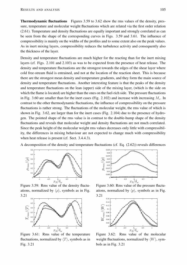
RESULTS AND ANALYSIS 105
Thermodynamic fluctuations Figures 3.59 to 3.62 show the rms values of the density, pres-sure, temperature and molecular weight fluctuations which are related via the first order relation(2.61). Temperature and density fluctuations are equally important and strongly correlated as canbe seen from the shape of the corresponding curves in Figs. 3.59 and 3.61. The influence ofcompressibility is mainly on the widths of the profiles and to some extent also on the peak values.As in inert mixing layers, compressibility reduces the turbulence activity and consequently alsothe thickness of the layer.
Density and temperature fluctuations are much higher for the reacting than for the inert mixinglayers (cf. Figs. 2.101 and 2.103) as was to be expected from the presence of heat release. Thedensity and temperature fluctuations are the strongest towards the edges of the shear layer wherecold free-stream fluid is entrained, and not at the location of the reaction sheet. This is becausethere are the strongest mean density and temperature gradients, and they form the main source ofdensity and temperature fluctuations. Another interesting feature is that the peaks of the densityand temperature fluctuations on the lean (upper) side of the mixing layer, (which is the side onwhich the flame is located) are higher than the ones on the fuel-rich side. The pressure fluctuationsin Fig. 3.60 are smaller than for the inert cases (Fig. 2.102) and increase with increasing Mc. Incontrast to the other thermodynamic fluctuations, the influence of compressibility on the pressurefluctuations is rather strong. The fluctuations of the molecular weight, the rms value of which isshown in Fig. 3.62, are larger than for the inert cases (Fig. 2.104) due to the presence of hydro-gen. The pointed shape of the rms value is in contrast to the double-hump shape of the densityfluctuations and reveals that molecular weight and density fluctuations are not much correlated.Since the peak height of the molecular weight rms values decreases only little with compressibil-ity, the differences in mixing behaviour are not expected to change much with compressibilitywhen heat release is present (cf. Sect. 3.4.4.3).
A decomposition of the density and temperature fluctuations (cf. Eq. (2.62)) reveals differences
x3/δω
ρrms/〈ρ〉
10.50-0.5-1
0.6
0.5
0.4
0.3
0.2
0.1
0
Figure 3.59: Rms value of the density fluctu-ations, normalized by 〈ρ〉, symbols as in Fig.3.21
x3/δω
p rms/〈p〉
10.50-0.5-1
0.045
0.04
0.035
0.03
0.025
0.02
0.015
0.01
0.005
0
Figure 3.60: Rms value of the pressure fluctu-ations, normalized by 〈p〉, symbols as in Fig.3.21
x3/δω
Trms/〈T〉
10.50-0.5-1
0.6
0.5
0.4
0.3
0.2
0.1
0
Figure 3.61: Rms value of the temperaturefluctuations, normalized by 〈T 〉, symbols as inFig. 3.21
x3/δω
Wrms/〈W〉
10.50-0.5-1
0.16
0.14
0.12
0.1
0.08
0.06
0.04
0.02
0
Figure 3.62: Rms value of the molecularweight fluctuations, normalized by 〈W 〉, sym-bols as in Fig. 3.21

106 3. DNS OF INFINITELY FAST REACTING COMPRESSIBLE TURBULENT SHEAR LAYERS
x3/δω
ρrms/〈ρ〉
10.50-0.5-1
0.6
0.5
0.4
0.3
0.2
0.1
0
Figure 3.63: Acoustic (solid line) and entropic part (dashed line) of the density fluctuations,normalized by 〈ρ〉, symbols as in Fig. 3.21
x3/δω
Trms/〈T〉
10.50-0.5-1
0.6
0.5
0.4
0.3
0.2
0.1
0
Figure 3.64: Acoustic (solid line) and entropic part (dashed line) of the temperature fluctuations,normalized by 〈T 〉, symbols as in Fig. 3.21
between the inert and the reacting mixing layers: For the latter ones, the entropic parts are muchlarger than the acoustic ones, even at higher convective Mach numbers (compare Figs. 3.63 and3.64 with Figs. 2.106 and 2.107).
Correlations of thermodynamic fluctuations A direct investigation of the correlation coeffi-cients R (ρ, p) and R (ρ, T ) (Figs. 3.65 and 3.66) confirms what was to be expected from theprevious paragraphs: There is only a weak correlation between density and pressure fluctuations,but a strong, inverse correlation of density and temperature fluctuations. Both correlation coeffi-cients are nearly uninfluenced by Mc.
x3/δω
R(ρ,p
)
10.50-0.5-1
1
0.5
0
-0.5
-1
Figure 3.65: Correlation coefficient R (ρ, p)
between pressure and density fluctuations,symbols as in Fig. 3.21
x3/δω
R(ρ,T
)
10.50-0.5-1
1
0.5
0
-0.5
-1
Figure 3.66: Correlation coefficient R (ρ, T )
between pressure and temperature fluctua-tions, symbols as in Fig. 3.21
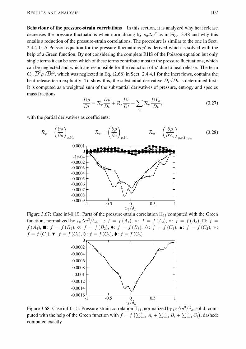
RESULTS AND ANALYSIS 107
Behaviour of the pressure-strain correlations In this section, it is analyzed why heat releasedecreases the pressure fluctuations when normalizing by ρ0∆u2 as in Fig. 3.48 and why thisentails a reduction of the pressure-strain correlations. The procedure is similar to the one in Sect.2.4.4.1: A Poisson equation for the pressure fluctuations p′ is derived which is solved with thehelp of a Green function. By not considering the complete RHS of the Poisson equation but onlysingle terms it can be seen which of these terms contribute most to the pressure fluctuations, whichcan be neglected and which are responsible for the reduction of p′ due to heat release. The termC6, D
2ρ′/Dt2, which was neglected in Eq. (2.68) in Sect. 2.4.4.1 for the inert flows, contains the
heat release term explicitly. To show this, the substantial derivative Dρ/Dt is determined first:It is computed as a weighted sum of the substantial derivatives of pressure, entropy and speciesmass fractions,
Dρ
Dt= Rp
Dp
Dt+Rs
Ds
Dt+∑
α
RαDYαDt
, (3.27)
with the partial derivatives as coefficients:
Rp =
(∂ρ
∂p
)
s,Yα
Rs =
(∂ρ
∂s
)
p,Yα
Rα =
(∂ρ
∂Yα
)
p,s,Yβ 6=α
(3.28)
x3/δω10.50-0.5-1
0.00010
-1e-04-0.0002-0.0003-0.0004-0.0005-0.0006-0.0007-0.0008-0.0009
Figure 3.67: Case inf-0.15: Parts of the pressure-strain correlation Π11 computed with the Greenfunction, normalized by ρ0∆u3/δω, +: f = f (A1), ×: f = f (A2), ∗: f = f (A3), �: f =
f (A4), �: f = f (B1), ◦: f = f (B2), •: f = f (B3), 4: f = f (C1), N: f = f (C2), O:f = f (C3), H: f = f (C4), ♦: f = f (C5), �: f = f (C5)
x3/δω10.50-0.5-1
0
-0.0002
-0.0004
-0.0006
-0.0008
-0.001
-0.0012
-0.0014
-0.0016
Figure 3.68: Case inf-0.15: Pressure-strain correlation Π11, normalized by ρ0∆u3/δω, solid: com-puted with the help of the Green function with f = f
(∑4i=1 Ai +
∑3i=1 Bi +
∑6i=1 Ci
), dashed:
computed exactly

108 3. DNS OF INFINITELY FAST REACTING COMPRESSIBLE TURBULENT SHEAR LAYERS
The partial derivative Rs is computed from the equation of state for ideal gas mixtures, Eq.(2.5) and the temperature dependence of the specific enthalpy at constant species mass fractions,dh = cpdT :
Rs =∂ρ
∂s=∂ρ
∂T· ∂T∂h· ∂h∂s
= − p
RGT 2· 1
cp· ∂h∂s
(3.29)
For the last term, ∂h/∂s, the Gibbs fundamental equation (A.38) is used, which simplifies todh = Tds for constant pressure and species mass fractions. Therefore ∂h/∂s = T and
Rs = − p
RGT 2· 1
cp· T = − ρ
cp. (3.30)
The partial derivativeRp is
Rp =∂ρ
∂p=
1∂p∂ρ
=1
c2, (3.31)
whereby Eq. (A.35) is taken into account. To computeRα, the relation
Rα =∂ρ
∂Yα=∂ρ
∂T· ∂T∂Yα
(3.32)
is useful. When computing ∂ρ/∂T with the help of the equation of state (2.5), it has to beconsidered that the gas constant of the mixture, RG, also depends on the mass fractions of the
x3/δω10.50-0.5-1
0.00020.0001
0-1e-04
-0.0002-0.0003-0.0004-0.0005-0.0006-0.0007-0.0008
Figure 3.69: Case inf-0.7: Parts of the pressure-strain correlation Π11 computed with the Greenfunction, normalized by ρ0∆u3/δω, symbols as in Fig. 3.67
x3/δω10.50-0.5-1
0.00020
-0.0002-0.0004-0.0006-0.0008-0.001
-0.0012-0.0014-0.0016
Figure 3.70: Case inf-0.7: Pressure-strain correlation Π11, normalized by ρ0∆u3/δω, solid: com-puted with the help of the Green function with f = f
(∑4i=1 Ai +
∑3i=1 Bi +
∑6i=1 Ci
), lines as
in Fig. 3.68

RESULTS AND ANALYSIS 109
species which themselves depend on the temperature:
∂ρ
∂T= − p
RG
T 2 − p
R2GT· ∂RG
∂Yα· ∂Yα∂T
= − p
RGT 2− p
R2GT· RWα
· ∂Yα∂T
(3.33)
Introducing this, as well as Eq. (A.46) into Eq. (3.32),
Rα = − p
RGT
(1
cpT
(µαWα
− hα)
+R
WαRG
)(3.34)
is obtained. The last term equals zero when the average molecular weight is constant [47]. Usingthis approximation (which is later justified by the good quality of the results), the final expressionfor Dρ/Dt, after introducing Eqs. (3.30), (3.31) and (3.34), as well as Dp/Dt and Ds/Dt (seeAppendix) into Eq. (3.27), is
Dρ
Dt=
1
c2
Dp
Dt+
1
cpT
(ρ∑
α
hαDYαDt
+∂qi∂xi− ∂ui∂xj
τij
)(3.35)
with DYαDt
computed from Eq. (3.15) for infinitely fast reacting flows. When neglecting moleculartransport terms, this becomes
Dρ
Dt≈ 1
c2
Dp
Dt− 1
cpTQ (3.36)
x3/δω10.50-0.5-1
1e-04
0
-0.0001
-0.0002
-0.0003
-0.0004
-0.0005
-0.0006
Figure 3.71: Case inf-1.1: Parts of the pressure-strain correlation Π11 computed with the Greenfunction, normalized by ρ0∆u3/δω, symbols as in Fig. 3.67
x3/δω10.50-0.5-1
0.0002
0
-0.0002
-0.0004
-0.0006
-0.0008
-0.001
-0.0012
Figure 3.72: Case inf-1.1: Pressure-strain correlation Π11, normalized by ρ0∆u3/δω, solid: com-puted with the help of the Green function with f = f
(∑4i=1 Ai +
∑3i=1 Bi +
∑6i=1 Ci
), lines as
in Fig. 3.68
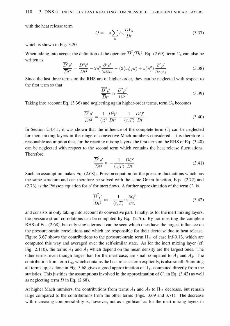
110 3. DNS OF INFINITELY FAST REACTING COMPRESSIBLE TURBULENT SHEAR LAYERS
with the heat release termQ = −ρ
∑
α
hαDYαDt
(3.37)
which is shown in Fig. 3.20.
When taking into accout the definition of the operator D2/Dt2, Eq. (2.69), term C6 can also be
written asD
2ρ′
Dt2=D2ρ′
Dt2− 2u′′j
∂2ρ′
∂t∂xj−(2〈ui〉fu′′j + u′′i u
′′j
) ∂2ρ′
∂xixj(3.38)
Since the last three terms on the RHS are of higher order, they can be neglected with respect tothe first term so that
D2ρ′
Dt2≈ D2ρ′
Dt2. (3.39)
Taking into account Eq. (3.36) and neglecting again higher-order terms, term C6 becomes
D2ρ′
Dt2=
1
〈c〉2D2p′
Dt2− 1
〈cpT 〉DQ′
Dt. (3.40)
In Section 2.4.4.1, it was shown that the influence of the complete term C6 can be neglectedfor inert mixing layers in the range of convective Mach numbers considered. It is therefore areasonable assumption that, for the reacting mixing layers, the first term on the RHS of Eq. (3.40)can be neglected with respect to the second term which contains the heat release fluctuations.Therefore,
D2ρ′
Dt2≈ − 1
〈cpT 〉DQ′
Dt. (3.41)
Such an assumption makes Eq. (2.68) a Poisson equation for the pressure fluctuations which hasthe same structure and can therefore be solved with the same Green function, Eqs. (2.72) and(2.73) as the Poisson equation for p′ for inert flows. A further approximation of the term C6 is
D2ρ′
Dt2≈ − 1
〈cpT 〉ui∂Q′
∂xi(3.42)
and consists in only taking into account its convective part. Finally, as for the inert mixing layers,the pressure-strain correlations can be computed by Eq. (2.76). By not inserting the completeRHS of Eq. (2.68), but only single terms it can be seen which ones have the largest influence onthe pressure-strain correlations and which are responsible for their decrease due to heat release.Figure 3.67 shows the contributions to the pressure-strain term Π11 of case inf-0.15, which arecomputed this way and averaged over the self-similar state. As for the inert mixing layer (cf.Fig. 2.110), the terms A1 and A2 which depend on the mean density are the largest ones. Theother terms, even though larger than for the inert case, are small compared to A1 and A2. Thecontribution from termC6, which contains the heat release term explicitly, is also small. Summingall terms up, as done in Fig. 3.68 gives a good approximation of Π11 computed directly from thestatistics. This justifies the assumptions involved in the approximation of C6 in Eq. (3.42) as wellas neglecting term D in Eq. (2.68).
At higher Mach numbers, the contributions from terms A1 and A2 to Π11 decrease, but remainlarge compared to the contributions from the other terms (Figs. 3.69 and 3.71). The decreasewith increasing compressibility is, however, not as significant as for the inert mixing layers in

RESULTS AND ANALYSIS 111
accordance with what has been observed for the complete pressure-strain rate. The good agree-ment between the curves in Figs. 3.70 and 3.72, which represent both, Π11 computed with thehelp of the Green function and Π11 computed directly from the statistics, shows, that acousticcontributions are not significant for the pressure-strain rate at convective Mach numbers up toMc = 1.1.
Compared to the inert cases, the complete pressure strain rate Π11 as well as the contributionsfrom terms A1 and A2 are reduced significantly by heat release. To find out, whether this is aconsequence of the reduced mean density (cf. Fig. 3.22), which appears as a factor in terms
x3/δω10.50-0.5-1
0.0005
0
-0.0005
-0.001
-0.0015
-0.002
-0.0025
-0.003
Figure 3.73: Case inf-0.15: Parts of the pressure-strain correlation Π11 computed with the Greenfunction and with constant density ρ0, normalized by ρ0∆u3/δω, symbols as in Fig. 3.67
x3/δω10.50-0.5-1
0.0005
0
-0.0005
-0.001
-0.0015
-0.002
-0.0025
-0.003
Figure 3.74: Case inf-0.7: Parts of the pressure-strain correlation Π11 computed with the Greenfunction and with constant density ρ0, normalized by ρ0∆u3/δω, symbols as in Fig. 3.67
x3/δω10.50-0.5-1
0.00020
-0.0002-0.0004-0.0006-0.0008-0.001
-0.0012-0.0014-0.0016-0.0018-0.002
Figure 3.75: Case inf-1.1: Parts of the pressure-strain correlation Π11 computed with the Greenfunction and with constant density ρ0, normalized by ρ0∆u3/δω, symbols as in Fig. 3.67
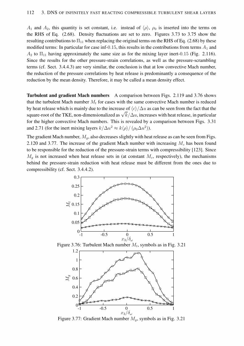
112 3. DNS OF INFINITELY FAST REACTING COMPRESSIBLE TURBULENT SHEAR LAYERS
A1 and A2, this quantity is set constant, i.e. instead of 〈ρ〉, ρ0 is inserted into the terms onthe RHS of Eq. (2.68). Density fluctuations are set to zero. Figures 3.73 to 3.75 show theresulting contributions to Π11 when replacing the original terms on the RHS of Eq. (2.68) by thesemodified terms: In particular for case inf-0.15, this results in the contributions from terms A1 andA2 to Π11 having approximately the same size as for the mixing layer inert-0.15 (Fig. 2.116).Since the results for the other pressure-strain correlations, as well as the pressure-scramblingterms (cf. Sect. 3.4.4.3) are very similar, the conclusion is that at low convective Mach number,the reduction of the pressure correlations by heat release is predominantly a consequence of thereduction by the mean density. Therefore, it may be called a mean density effect.
Turbulent and gradient Mach numbers A comparison between Figs. 2.119 and 3.76 showsthat the turbulent Mach number Mt for cases with the same convective Mach number is reducedby heat release which is mainly due to the increase of 〈c〉/∆u as can be seen from the fact that thesquare-root of the TKE, non-dimensionalized as
√k/∆u, increases with heat release, in particular
for the higher convective Mach numbers. This is revealed by a comparison between Figs. 3.31and 2.71 (for the inert mixing layers k/∆u2 ≈ k〈ρ〉/ (ρ0∆u2)).
The gradient Mach number,Mg, also decreases slightly with heat release as can be seen from Figs.2.120 and 3.77. The increase of the gradient Mach number with increasing Mc has been foundto be responsible for the reduction of the pressure-strain terms with compressibility [123]. SinceMg is not increased when heat release sets in (at constant Mc, respectively), the mechanismsbehind the pressure-strain reduction with heat release must be different from the ones due tocompressibility (cf. Sect. 3.4.4.2).
x3/δω
Mt
10.50-0.5-1
0.3
0.25
0.2
0.15
0.1
0.05
0
Figure 3.76: Turbulent Mach number Mt, symbols as in Fig. 3.21
x3/δω
Mg
10.50-0.5-1
1.2
1
0.8
0.6
0.4
0.2
0
Figure 3.77: Gradient Mach number Mg, symbols as in Fig. 3.21

RESULTS AND ANALYSIS 113
Mg
Mt
1.210.80.60.40.20
0.450.4
0.350.3
0.250.2
0.150.1
0.050
Figure 3.78: Turbulent Mach number Mt plotted as a function of the gradient Mach number Mg.Symbols as in Fig. 3.21, solid line: Mt = 0.350Mg, dashed line: Mt = 0.210Mg
As for the inert mixing layers, there is an approximately linear correlation between Mt and Mg
for the reacting mixing layers as the scatter plot in Fig. 3.78 shows. However, the slope of thelinear relation is different from that for the inert cases (cf. Fig. 2.121) due to different behaviourof Mt and Mg with heat release.
Spectra Figure 3.79 shows the one-dimensional, streamwise spectrum of the velocity u1 afteraveraging over directions x2 and x3. Even though the resolution of the reacting cases is lowerthan for the inert cases (cf. Fig. 2.122), which causes the lower range of wavenumbers on thehorizontal axis, no signs of under-resolution are visible, and the energy fall-off in all cases extendssmoothly over several orders of magnitude. The higher the wavenumber, the stronger is the effectof heat release which manifests itself in a lower energy content. As for the inert mixing layers,compressibility decreases the energy in the highest wavenumbers resulting in a visible increaseof the dominant length scales (cf. Sect. 3.4.1). While the changes from Mc = 0.15 to Mc = 0.7
are quite strong, an asymptotic behaviour sets in when increasing Mc further.
All scales of the TKE are affected by increasing Mc when heat release is present (Fig. 3.80).Less energy in large and intermediate scales is observed and means that there is less transport ofmomentum and scalar quantities by the turbulence. Consequences are smaller growth rates andless entrainment of outside fluid due to compressibility (cf. Sect. 3.4.4.4).
In the one-dimensional dissipation spectra in Fig. 3.81, the peak position is rather uninfluenced by
k1δω,0
Eu
1010.1
1
1e-05
1e-10
1e-15
1e-20
Figure 3.79: One-dimensional, streamwise spectrum of u1/∆u at the beginning of the self-similarstate, solid: inf-0.15, dashed: inf-0.7, dotted: inf-1.1
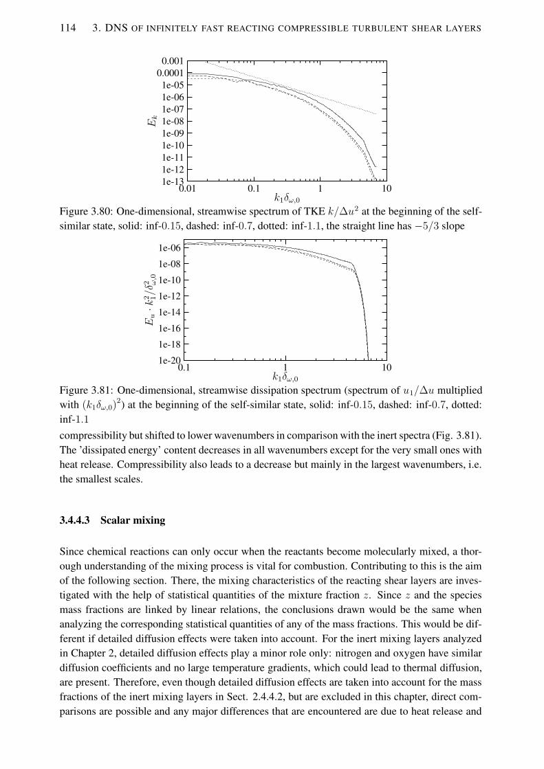
114 3. DNS OF INFINITELY FAST REACTING COMPRESSIBLE TURBULENT SHEAR LAYERS
k1δω,0
Ek
1010.10.01
0.0010.00011e-051e-061e-071e-081e-091e-101e-111e-121e-13
Figure 3.80: One-dimensional, streamwise spectrum of TKE k/∆u2 at the beginning of the self-similar state, solid: inf-0.15, dashed: inf-0.7, dotted: inf-1.1, the straight line has −5/3 slope
k1δω,0
Eu·k
2 1/δ
2 ω,0
1010.1
1e-06
1e-08
1e-10
1e-12
1e-14
1e-16
1e-18
1e-20
Figure 3.81: One-dimensional, streamwise dissipation spectrum (spectrum of u1/∆u multipliedwith (k1δω,0)2) at the beginning of the self-similar state, solid: inf-0.15, dashed: inf-0.7, dotted:inf-1.1compressibility but shifted to lower wavenumbers in comparison with the inert spectra (Fig. 3.81).The ’dissipated energy’ content decreases in all wavenumbers except for the very small ones withheat release. Compressibility also leads to a decrease but mainly in the largest wavenumbers, i.e.the smallest scales.
3.4.4.3 Scalar mixing
Since chemical reactions can only occur when the reactants become molecularly mixed, a thor-ough understanding of the mixing process is vital for combustion. Contributing to this is the aimof the following section. There, the mixing characteristics of the reacting shear layers are inves-tigated with the help of statistical quantities of the mixture fraction z. Since z and the speciesmass fractions are linked by linear relations, the conclusions drawn would be the same whenanalyzing the corresponding statistical quantities of any of the mass fractions. This would be dif-ferent if detailed diffusion effects were taken into account. For the inert mixing layers analyzedin Chapter 2, detailed diffusion effects play a minor role only: nitrogen and oxygen have similardiffusion coefficients and no large temperature gradients, which could lead to thermal diffusion,are present. Therefore, even though detailed diffusion effects are taken into account for the massfractions of the inert mixing layers in Sect. 2.4.4.2, but are excluded in this chapter, direct com-parisons are possible and any major differences that are encountered are due to heat release and

RESULTS AND ANALYSIS 115
compressibility and not to diffusion effects.
Mean profile and variance Figure 3.82 shows the Favre averaged profiles of the mixture frac-tion. The profiles at the various convective Mach numbers are close to each other, and it is hardto tell whether the differences are larger than those for the velocity profiles of the inert mixinglayers. Due to the larger density fluctuations, the differences between the Favre and the Reynoldsquantities are larger for the reacting mixing layers than for the inert ones. Figure 3.83 demon-strates this for the mixture fraction of the inert-0.15 case. It can be seen that the Favre averagedprofile is above the Reynolds averaged one on the fuel side of the mixing layer and that the oppo-site is true on the oxidizer side. This is in agreement with the observations of Pantano et al. [124]and can be explained when considering that
〈z〉f − 〈z〉 =〈ρ′z′〉〈ρ〉 . (3.43)
The correlation between the density and the mixture fraction fluctuations is positive on the fuelside since higher ρ (colder fluid) is associated there with higher z (more fuel). On the oxidizerside, the correlation is negative since higher ρ corresponds to more oxygen and therefore lowerz. A similar relation has been observed for the Favre and Reynolds averaged velocity profiles inSect. 3.4.4.2.
Figure 3.84 shows the mixture fraction variance for the reacting mixing layers. Comparing thisfigure with the corresponding one for the inert mixing layers, Fig. 2.126, it is obvious that theinfluence of differentMc is less pronounced for the reacting mixing layers than for the inert ones -
x3/δω
〈z〉 f
10.50-0.5-1
10.90.80.70.60.50.40.30.20.1
0
Figure 3.82: Favre averaged mixture fraction, ∗: inf-0.15, �: inf-0.7, ◦: inf-1.1
x3/δω10.50-0.5-1
10.90.80.70.60.50.40.30.20.1
0
Figure 3.83: Case inert-0.15, solid: 〈z〉f , dashed: 〈z〉

116 3. DNS OF INFINITELY FAST REACTING COMPRESSIBLE TURBULENT SHEAR LAYERS
x3/δω
〈z′′2〉 f
10.50-0.5-1
0.050.0450.04
0.0350.03
0.0250.02
0.0150.01
0.0050
Figure 3.84: Variance of the mixture fraction, symbols as in Fig. 3.82
x3/δω
〈ρz′′2〉/ρ
0
10.50-0.5-1
0.016
0.014
0.012
0.01
0.008
0.006
0.004
0.002
0
Figure 3.85: Variance of the mixture fraction, normalized by ρ0/〈ρ〉, symbols as in Fig. 3.82
a feature that has already been observed for various other statistical quantities in Sect. 3.4.4.2. Inparticular, the decrease of the peak value with increasing Mc is relatively small and no significantchange in shape is visible. None of the variance profiles of the reacting mixing layers has adouble hump as was observed for case inert-0.15. Since the double hump in this case is due toengulfment at the edges of the mixing layer, weak engulfment is expected for the reacting layers.This is confirmed by the results in Sect. 3.4.4.4. The variance profiles are more pointed for thereacting cases than for the inert ones (cf. Fig. 2.126), and the peak value is shifted towards theside of the mixing layer where the stoichiometric surface is located.
When comparing the level of the scalar fluctuations, it is useful to take into account the reductionof the density which is done by a different normalization, applied in Fig. 3.85. A correspondingnormalization has been used for the Reynolds stresses and the TKE in Sect. 3.4.4.2 and hasrevealed that their reduction by heat release is predominantly a mean density effect. This is alsothe case for the scalar variance, since with the normalization in Fig. 3.85 the scalar fluctuations arereduced by heat release (compare with Fig. 2.126), contrarily to what is observed from comparingFigs. 3.84 and 2.126. Note that a change in normalization would not alter the profiles of the scalarvariance of the inert mixing layers much since 〈ρ〉/ρ0 ≈ 1 in these cases. Therefore, both, Figs.3.84 and 3.85, can be compared to Fig. 2.126.
Comparing the effects that heat release has on the scalar variance with its effects on the TKE(Figs. 2.71, 3.30 and 3.31), it can be concluded that the influence of heat release on the shape ofthe profiles is larger for the scalar variance than for the TKE while the peak value of the TKE isstronger influenced than that of the scalar variance (appropriate normalization provided). Pantanoet al. [124] made similar observations and concluded that the effect of heat release on scalar and

RESULTS AND ANALYSIS 117
velocity quantities is approximately the same when integrated across the shear layer.
Scalar pdfs The mixture fraction pdfs of the three reacting test cases in Figs. 3.86 to 3.88 takenin planes with different 〈z〉 show a marching behaviour with the most probable value varyingacross the mixing layer. This behaviour is even more pronounced than for the inert mixing layers(cf. Figs. 2.127 to 2.129) since the so-called mixed-fluid peak of the extreme pdfs is situatedcloser to 〈z〉 of that plane out of which the respective pdf is taken. From the marching behaviourof the pdfs and the fact that only the two extreme pdfs on each side are bi-modal, i.e. have anintermittency peak in addition to the mixed-fluid peak, it is expected that the fluid gets mixed intothe layer at the edges rather than engulfed (cf. Sect. 3.4.4.4). In particular at lowMc, the bi-modalshape is encountered for fewer pdfs than it is the case for the inert mixing layers which showsthat the external intermittency decreases with heat release. This observation is in agreement withthe results of Pantano et al. [124] and with those in Sect. 3.4.4.4.
The probability to encounter free-stream fluid in the reacting mixing layer in the planes with〈z〉 = 0.2 and 〈z〉 = 0.8 decreases with increasing compressibility. However, in contrast tothe inert mixing layers, the probability to encounter such fluid in the planes with 〈z〉 = 0.3 and〈z〉 = 0.7 is nearly independent of the Mach number. It can be concluded that for the entrainment,as for other features that have already been investigated in the previous sections, the influence ofcompressibility on inert mixing layers is larger than on reacting mixing layers.
z
10.90.80.70.60.50.40.30.20.10
6
5
4
3
2
1
0
Figure 3.86: Case inf-0.15: pdfs of mixture fraction in planes with various 〈z〉, +: 0.1,×: 0.2, ∗:0.3, �: 0.4, �: 0.5, ◦: 0.6, •: 0.7,4: 0.8, N: 0.9
z
10.90.80.70.60.50.40.30.20.10
6
5
4
3
2
1
0
Figure 3.87: Case inf-0.7: pdfs of mixture fraction in planes with various 〈z〉, +: 0.1, ×: 0.2, ∗:0.3, �: 0.4, �: 0.5, ◦: 0.6, •: 0.7,4: 0.8, N: 0.9

118 3. DNS OF INFINITELY FAST REACTING COMPRESSIBLE TURBULENT SHEAR LAYERS
z
10.90.80.70.60.50.40.30.20.10
6
5
4
3
2
1
0
Figure 3.88: Case inf-1.1: pdfs of mixture fraction in planes with various 〈z〉, +: 0.1, ×: 0.2, ∗:0.3, �: 0.4, �: 0.5, ◦: 0.6, •: 0.7,4: 0.8, N: 0.9
x3/δω
10.90.80.70.60.50.40.30.20.10
4
3.5
3
2.5
2
1.5
1
0.5
0
Figure 3.89: Pdfs of mixture fraction in the plane with 〈z〉 = 0.3 (solid) and 〈z〉 = 0.5 (dashed),symbols as in Fig. 3.82
The pointed shape of the scalar variance in Fig. 3.84 and the shift of its peak away from the centerof the mixing layer can be related with the different shapes that the mixture fraction pdfs have atthe various locations across the mixing layer, as e.g. displayed in Fig. 3.86: The pdfs that aretaken from the lower, oxygen side of the mixing layer are broader, i.e. have a higher variancethan the ones taken from the upper, fuel side. This is consistent with the maximum of the scalarvariance being shifted towards the oxygen side, i.e. towards the plane with the stoichiometricvalue 〈z〉 = 0.3.
In Fig. 3.89, the scalar pdfs taken in the planes with 〈z〉 = 0.3 and 〈z〉 = 0.5 are plotted fordifferent convective Mach numbers. Again, the relatively weak influence of compressibility isvisible.
Mixing efficiency The mixing efficiency, which measures the mixing of the fluid in the layerat the molecular level and reveals how much free-stream fluid is present, is computed for themixture fraction by
δMδz
=1
δz
∫ ∞
0
dx3
∫ 1−ε
ε
dzP (z, x3) (3.44)
where δz denotes the 99% scalar thickness. This definition has been suggested by Freund et al.[64]. Fig. 3.90 shows the mixing efficiency as a function of Mc for the reacting mixing layers.The curves for two different values of the small parameter ε, which determines what kind of fluidis considered to be pure, are shown. It can be seen that the mixing efficiency increases with
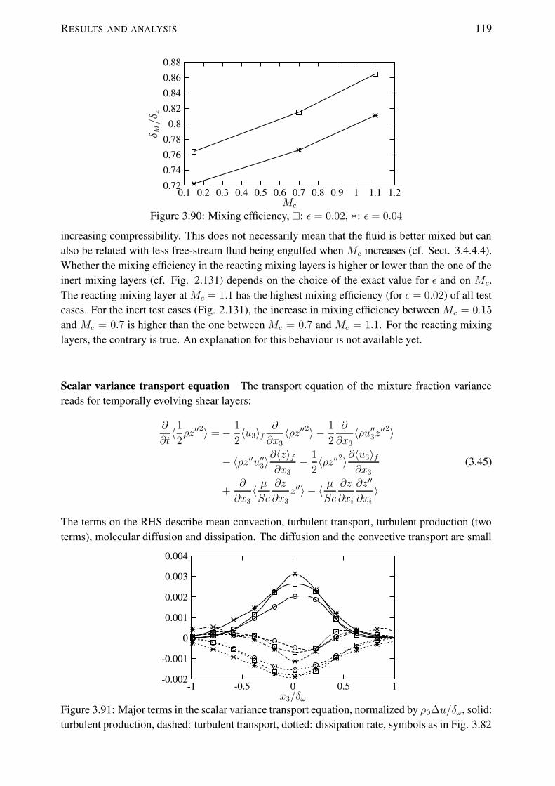
RESULTS AND ANALYSIS 119
Mc
δ M/δz
1.21.110.90.80.70.60.50.40.30.20.1
0.88
0.86
0.84
0.82
0.8
0.78
0.76
0.74
0.72
Figure 3.90: Mixing efficiency, �: ε = 0.02, ∗: ε = 0.04
increasing compressibility. This does not necessarily mean that the fluid is better mixed but canalso be related with less free-stream fluid being engulfed when Mc increases (cf. Sect. 3.4.4.4).Whether the mixing efficiency in the reacting mixing layers is higher or lower than the one of theinert mixing layers (cf. Fig. 2.131) depends on the choice of the exact value for ε and on Mc.The reacting mixing layer at Mc = 1.1 has the highest mixing efficiency (for ε = 0.02) of all testcases. For the inert test cases (Fig. 2.131), the increase in mixing efficiency between Mc = 0.15
and Mc = 0.7 is higher than the one between Mc = 0.7 and Mc = 1.1. For the reacting mixinglayers, the contrary is true. An explanation for this behaviour is not available yet.
Scalar variance transport equation The transport equation of the mixture fraction variancereads for temporally evolving shear layers:
∂
∂t〈12ρz′′
2〉 =− 1
2〈u3〉f
∂
∂x3〈ρz′′2〉 − 1
2
∂
∂x3〈ρu′′3z′′2〉
− 〈ρz′′u′′3〉∂〈z〉f∂x3
− 1
2〈ρz′′2〉∂〈u3〉f
∂x3
+∂
∂x3〈 µSc
∂z
∂x3z′′〉 − 〈 µ
Sc
∂z
∂xi
∂z′′
∂xi〉
(3.45)
The terms on the RHS describe mean convection, turbulent transport, turbulent production (twoterms), molecular diffusion and dissipation. The diffusion and the convective transport are small
x3/δω10.50-0.5-1
0.004
0.003
0.002
0.001
0
-0.001
-0.002
Figure 3.91: Major terms in the scalar variance transport equation, normalized by ρ0∆u/δω, solid:turbulent production, dashed: turbulent transport, dotted: dissipation rate, symbols as in Fig. 3.82

120 3. DNS OF INFINITELY FAST REACTING COMPRESSIBLE TURBULENT SHEAR LAYERS
x3/δω10.50-0.5-1
0.0005
0
-0.0005
-0.001
-0.0015
-0.002
-0.0025
Figure 3.92: Parts of the scalar dissipation rate, solid: −〈 µSc
∂z∂xj
∂z∂xj〉, dashed: 〈 µ
Sc∂z∂xj〉∂〈z〉f∂xj
, nor-malized by ρ0∆u/δω, symbols as in Fig. 3.82
compared to the other terms which are shown in Fig. 3.91. They are all reduced by compressibil-ity and heat release (cf. Fig. 2.132) with the reduction due to compressibility being weaker whenheat release is present.
The dissipation rate can also be written as
εz = −〈 µSc
∂z
∂xi
∂z′′
∂xi〉 = −〈 µ
Sc
∂z
∂xj
∂z
∂xj〉+ 〈 µ
Sc
∂z
∂xj〉∂〈z〉f∂xj
(3.46)
with the second term being negligible compared to the first one (Fig. 3.92). Therefore, εz can beapproximated as:
εz ≈ −〈µ
Sc
∂z
∂xj
∂z
∂xj〉 (3.47)
Scalar fluxes The streamwise scalar flux, 〈ρu′′1z′′〉, and the transverse scalar flux, 〈ρu′′3z′′〉, areshown in Figs. 3.93 and 3.94. They are considerably smaller than for the inert cases (cf. Figs.2.134 and 2.135). The fact that the fluxes in the inert and reacting cases have different signsresults from the different signs of the mean scalar gradient. The spanwise scalar flux is negli-gible compared to the other fluxes and therefore not shown. As for the inert mixing layers, thetransverse scalar flux is more sensitive to an increase in Mc and reduces more strongly than thestreamwise scalar flux.
x3/δω
〈ρu′′ 1z′′ 〉/
(ρ0∆u
)
10.50-0.5-1
0.0010
-0.001-0.002-0.003-0.004-0.005-0.006-0.007-0.008
Figure 3.93: Scalar flux 〈ρu′′1z′′〉, normalized by ρ0∆u, symbols as in Fig. 3.82
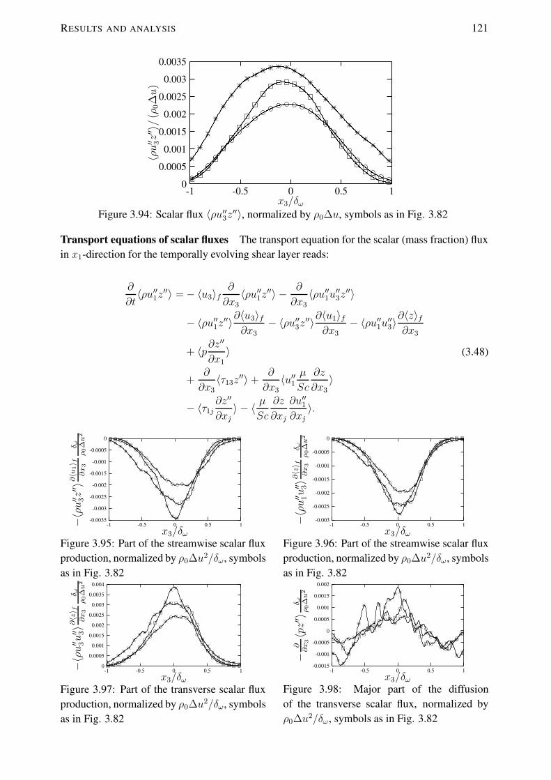
RESULTS AND ANALYSIS 121
x3/δω
〈ρu′′ 3z′′ 〉/
(ρ0∆u
)
10.50-0.5-1
0.0035
0.003
0.0025
0.002
0.0015
0.001
0.0005
0
Figure 3.94: Scalar flux 〈ρu′′3z′′〉, normalized by ρ0∆u, symbols as in Fig. 3.82
Transport equations of scalar fluxes The transport equation for the scalar (mass fraction) fluxin x1-direction for the temporally evolving shear layer reads:
∂
∂t〈ρu′′1z′′〉 =− 〈u3〉f
∂
∂x3
〈ρu′′1z′′〉 −∂
∂x3
〈ρu′′1u′′3z′′〉
− 〈ρu′′1z′′〉∂〈u3〉f∂x3
− 〈ρu′′3z′′〉∂〈u1〉f∂x3
− 〈ρu′′1u′′3〉∂〈z〉f∂x3
+ 〈p∂z′′
∂x1〉
+∂
∂x3〈τ13z
′′〉+∂
∂x3〈u′′1
µ
Sc
∂z
∂x3〉
− 〈τ1j∂z′′
∂xj〉 − 〈 µ
Sc
∂z
∂xj
∂u′′1∂xj〉.
(3.48)
x3/δω
−〈ρu′′ 3z′′ 〉∂〈u
1〉 f
∂x
3
δ ωρ
0∆u
2
10.50-0.5-1
0
-0.0005
-0.001
-0.0015
-0.002
-0.0025
-0.003
-0.0035
Figure 3.95: Part of the streamwise scalar fluxproduction, normalized by ρ0∆u2/δω, symbolsas in Fig. 3.82
x3/δω
−〈ρu′′ 1u′′ 3〉∂〈z〉 f
∂x
3
δ ωρ
0∆u
2
10.50-0.5-1
0
-0.0005
-0.001
-0.0015
-0.002
-0.0025
-0.003
Figure 3.96: Part of the streamwise scalar fluxproduction, normalized by ρ0∆u2/δω, symbolsas in Fig. 3.82
x3/δω
−〈ρu′′ 3u′′ 3〉∂〈z〉 f
∂x
3
δ ωρ
0∆u
2
10.50-0.5-1
0.004
0.0035
0.003
0.0025
0.002
0.0015
0.001
0.0005
0
Figure 3.97: Part of the transverse scalar fluxproduction, normalized by ρ0∆u2/δω, symbolsas in Fig. 3.82
x3/δω
−∂∂x
3〈pz′′ 〉
δ ωρ
0∆u
2
10.50-0.5-1
0.002
0.0015
0.001
0.0005
0
-0.0005
-0.001
-0.0015
Figure 3.98: Major part of the diffusionof the transverse scalar flux, normalized byρ0∆u2/δω, symbols as in Fig. 3.82
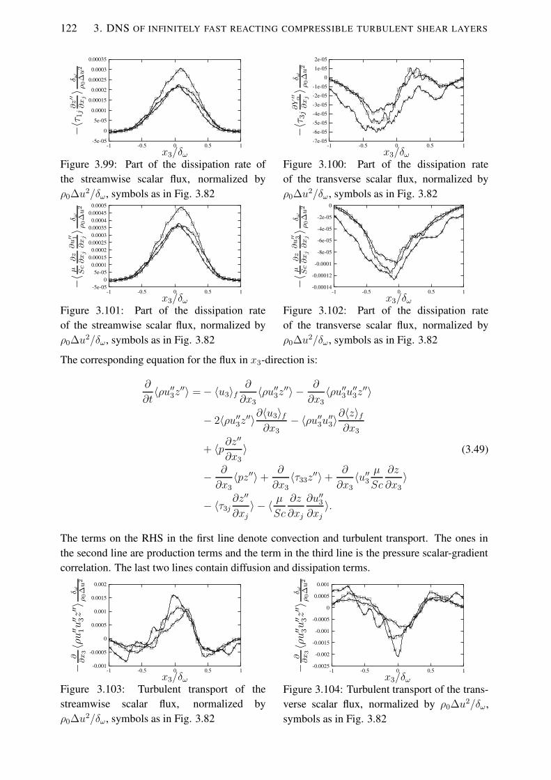
122 3. DNS OF INFINITELY FAST REACTING COMPRESSIBLE TURBULENT SHEAR LAYERS
x3/δω
−〈τ 1j∂z′′
∂xj〉
δ ωρ
0∆u
2
10.50-0.5-1
0.00035
0.0003
0.00025
0.0002
0.00015
0.0001
5e-05
0
-5e-05
Figure 3.99: Part of the dissipation rate ofthe streamwise scalar flux, normalized byρ0∆u2/δω, symbols as in Fig. 3.82
x3/δω
−〈τ 3j∂Y′′ α
∂xj〉
δ ωρ
0∆u
2
10.50-0.5-1
2e-05
1e-05
0
-1e-05
-2e-05
-3e-05
-4e-05
-5e-05
-6e-05
-7e-05
Figure 3.100: Part of the dissipation rateof the transverse scalar flux, normalized byρ0∆u2/δω, symbols as in Fig. 3.82
x3/δω
−〈µ Sc∂z
∂xj
∂u′′ 1
∂xj〉
δ ωρ
0∆u
2
10.50-0.5-1
0.00050.00045
0.00040.00035
0.00030.00025
0.00020.00015
0.00015e-05
0-5e-05
Figure 3.101: Part of the dissipation rateof the streamwise scalar flux, normalized byρ0∆u2/δω, symbols as in Fig. 3.82
x3/δω−〈
µ Sc∂z
∂xj
∂u′′ 3
∂xj〉
δ ωρ
0∆u
2
10.50-0.5-1
0
-2e-05
-4e-05
-6e-05
-8e-05
-0.0001
-0.00012
-0.00014
Figure 3.102: Part of the dissipation rateof the transverse scalar flux, normalized byρ0∆u2/δω, symbols as in Fig. 3.82
The corresponding equation for the flux in x3-direction is:
∂
∂t〈ρu′′3z′′〉 =− 〈u3〉f
∂
∂x3〈ρu′′3z′′〉 −
∂
∂x3〈ρu′′3u′′3z′′〉
− 2〈ρu′′3z′′〉∂〈u3〉f∂x3
− 〈ρu′′3u′′3〉∂〈z〉f∂x3
+ 〈p∂z′′
∂x3
〉
− ∂
∂x3
〈pz′′〉+∂
∂x3
〈τ33z′′〉+
∂
∂x3
〈u′′3µ
Sc
∂z
∂x3
〉
− 〈τ3j∂z′′
∂xj〉 − 〈 µ
Sc
∂z
∂xj
∂u′′3∂xj〉.
(3.49)
The terms on the RHS in the first line denote convection and turbulent transport. The ones inthe second line are production terms and the term in the third line is the pressure scalar-gradientcorrelation. The last two lines contain diffusion and dissipation terms.
x3/δω
−∂∂x
3〈ρu′′ 1u′′ 3z′′ 〉
δ ωρ
0∆u
2
10.50-0.5-1
0.002
0.0015
0.001
0.0005
0
-0.0005
-0.001
Figure 3.103: Turbulent transport of thestreamwise scalar flux, normalized byρ0∆u2/δω, symbols as in Fig. 3.82
x3/δω
−∂∂x
3〈ρu′′ 3u′′ 3z′′ 〉
δ ωρ
0∆u
2
10.50-0.5-1
0.001
0.0005
0
-0.0005
-0.001
-0.0015
-0.002
-0.0025
Figure 3.104: Turbulent transport of the trans-verse scalar flux, normalized by ρ0∆u2/δω,symbols as in Fig. 3.82

RESULTS AND ANALYSIS 123
x3/δω
〈p′∂z′′
∂x
1〉
δ ωρ
0∆u
2
10.50-0.5-1
0.0045
0.004
0.0035
0.003
0.0025
0.002
0.0015
0.001
0.0005
0
Figure 3.105: Pressure-scrambling termin streamwise direction, normalized byρ0∆u2/δω, symbols as in Fig. 3.82
x3/δω
〈p′∂z′′
∂x
3〉
δ ωρ
0∆u
2
10.50-0.5-1
0.0010.0005
0-0.0005
-0.001-0.0015
-0.002-0.0025
-0.003-0.0035
-0.004
Figure 3.106: Pressure-scrambling term intransverse direction, normalized by ρ0∆u2/δω,symbols as in Fig. 3.82
The pressure scalar gradient correlation can also be written as
〈p∂z′′
∂x1
〉 = 〈p′∂z′′
∂x1
〉, (3.50)
in x1-direction and in x3 direction,
〈p∂z′′
∂x3〉 = 〈p〉∂〈z〉
∂x3− 〈p〉∂〈z〉f
∂x3+ 〈p′∂z
′′
∂x3〉 (3.51)
with the last term in each expression being the pressure-scrambling term Πzi.
The major terms in these equations are the production, the diffusion, the dissipation rates andthe turbulent transport as well as the pressure-scrambling term. They are shown in Figs. 3.95 to3.106 and are smaller than for the inert cases. While the production rates, the dissipation rate, thediffusion and the turbulent transport are more pointed in the center than the corresponding termsfor the inert cases, the pressure-scrambling term has a similar shape. All terms in the reactingcases show the already expected behaviour of being less sensitive to changes in Mc than withoutheat release which makes the influence of heat release stronger at low Mc. Moreover, most ofthe terms are damped by compressibility, except for the two parts of the dissipation rate of thestreamwise scalar flux shown in Figs. 3.99 and 3.101.
Spectra The scalar energy spectra in Fig. 3.107 and the scalar dissipation spectra in Fig. 3.108of the reacting test cases are similar to the inert ones (cf. Figs. 2.157 and 2.158) in the largescales but contain less energy in the small scales. This is in agreement with the smoother scalar
k1δω,0
Ez
1010.10.01
1
0.01
0.0001
1e-06
1e-08
1e-10
Figure 3.107: One-dimensional, streamwise spectrum of the mixture fraction z, solid: inert-0.15,dashed: inert-0.7, dotted: inert-1.1, the straight line has −5/3 slope

124 3. DNS OF INFINITELY FAST REACTING COMPRESSIBLE TURBULENT SHEAR LAYERS
k1δω,0
Ez·k
2 1/δ
2 ω,0
1010.1
0.0001
1e-05
1e-06
1e-07
1e-08
1e-09
1e-10
Figure 3.108: One-dimensional dissipation spectrum of the mixture fraction z (spectrum of zmultiplied with (k1δω,0)2), solid: inert-0.15, dashed: inert-0.7, dotted: inert-1.1
fields that have been noticed in Sect. 3.4.1. Additionally, the peaks of the dissipation spectrafor the reacting cases are situated at higher wavenumbers than for the inert cases. Due to thecoarser resolution of the reacting test cases, the range of wavenumbers on the horizontal axesin Figs. 3.107 and 3.108 do not extend to such high wavenumbers as in Fig. 2.157 and 2.158.Nevertheless, the energy fall-off is smooth over several orders of magnitudes and no signs ofspurious energy accumulation in the highest wavenumbers are visible. In contrast to what hasbeen observed from the inert test cases, changes with Mc are only observed between Mc = 0.15
and Mc = 0.7 and not when rising Mc further. The peak of the dissipation spectrum is ratheruninfluenced by compressibility.
3.4.4.4 Entrainment
Knowledge of the entrainment mechanisms and their changes with heat release and combustion isparticularly important for reacting flows since the amount of chemical product formed as a resultof mixing is limited by the amount of reactant species entrained into the layer [72]. A hint that theentrainment of outside fluid is reduced by heat release is given by the fact that the mixing layergrowth rate decreases when heat release is present inspite of a possible increase by displacementeffects due to thermal expansion. Hermanson and Dimotakis [72] used different methods, e.g.integral and geometrical formulae, to compute the entrainment into mixing layers with differentdensity reductions by heat release and confirmed this suggestion.
One feature concerning the entrainment that cannot be investigated with the present, temporallyevolving mixing layer configuration is the entrainment ratio, i.e. the average amount of fluidentrained into a spatially evolving mixing layer from the high-speed side divided by the averageamount of fluid entrained from the low-speed side. Hermanson and Dimotakis [72] showed itsreduction with heat release, and Miller et al. [114] found it to be reduced further with compress-ibility, which is in agreement with the results of Hall et al. [70] for the inert mixing layer. Thismeans that the overall stoichiometry of the mixing layer is affected by both, compressibility andheat release, which can also have feedback effects on the heat release characteristics.
Measurement of volumes The distinction between the mixing layer and its surroundings aswell as between the mixed volume and the engulfed volume within the mixing layer is made

RESULTS AND ANALYSIS 125
here again with the help of vorticity and scalar thresholds. The determination of the differentvolumes (mixing layer, mixed and engulfed volume) is the same as described previously for theinert mixing layers (cf. Sect. 2.4.4.3). The threshold values used for the reacting mixing layerdo not differ from those used for the inert test cases: z = 0.05 and 0.95 for the scalar (here themixture fraction) and ω = 0.1〈ωmax〉 for the vorticity.
Figures 3.109 and 3.110 show the mixing layer volume and the engulfed volume for the reactingflow cases through a part of the self-similar state. To facilitate comparison with the correspondingfigures for the inert mixing layers (Figs. 2.161 and 2.162) only part of the self-similar state isshown. However, the growth of mixing layer and engulfed volume that is visible during thetime period shown continues throughout the self-similar state, and the growth rates nearly remainconstant. The growth of the mixing layer decreases with increasing Mc, but the decrease, inparticular between Mc = 0.15 and Mc = 0.7, is not as pronounced as without combustion. Intotal, the growth rates for the reacting mixing layers are smaller than for the inert ones, which ismost obvious for the test cases at Mc = 0.15 and which is in agreement with other authors whofound the entrainment being reduced with heat release [72].
(t− tB) ·∆u/δω,0120100806040200
1.2
1
0.8
0.6
0.4
0.2
0
Figure 3.109: Based on vorticity thresholds: Mixing layer volume Vml (solid) and engulfed vol-ume Ven (dashed) vs. the normalized time passed since the beginning of the self-similar state attB . Volumes are normalized with the mixing layer volume at the beginning of the self-similarstate, Vml,B, ∗: inf-0.15, �: inf-0.7, ◦: inf-1.1
(t− tB) ·∆u/δω,0120100806040200
1.2
1
0.8
0.6
0.4
0.2
0
Figure 3.110: Based on mixture fraction thresholds: Mixing layer volume Vml (solid) and en-gulfed volume Ven (dashed) vs. the normalized time passed since the beginning of the self-similarstate at tB . Volumes are normalized with the mixing layer volume at the beginning of the self-similar state, Vml,B . Symbols as in Fig. 3.109

126 3. DNS OF INFINITELY FAST REACTING COMPRESSIBLE TURBULENT SHEAR LAYERS
The engulfed volume constitutes only a small part of the mixing layer: about 4 % for case inf-0.15, 2.5 % for case inf-0.7 and 1.5 % for case inf-1.1, which is smaller than for the inert cases atthe same convective Mach number, a tendency which is in agreement with the results of Planche& Reynolds [141].
A comparison between Fig. 3.109 and Fig. 3.110 shows that it is not of much importance for thevolumes and their growth rates whether mixture fraction thresholds are used instead of vorticitythresholds.
Visual thickness Figure 3.111 shows the visual thicknesses δvis and thicknesses derived fromthe mixing layer volume, δvol (cf. Sect. 2.4.4.3), for the reacting mixing layers. Even though areduction of the respective growth rates withMc can be observed it is not as strong as for the inertmixing layers (Fig. 2.163), the growth of which is also faster. As explained in the correspondingsection about the visual thickness of the inert mixing layers, the distance between the curves ofthe visual thickness and the ones of the thickness derived from the mixing layer volume is affectedby intermittency. As in inert mixing layers, the intermittency decreases with compressibility inreacting ones, i.e. δvis and δvol in Fig. 3.111 become closer.
In Fig. 3.112, the mixture fraction thresholds are used to determine δvis and δvol which leads to
(t− tB) ·∆u/δω,0120100806040200
1.21.15
1.11.05
10.95
0.90.85
0.80.75
Figure 3.111: Based on vorticity thresholds: Thickness computed from mixing layer volume δvol(solid) and visual thickness δvis (dashed). Thicknesses are normalized by the visual thickness atthe beginning of the self-similar state, δvis,B. Symbols as in Fig. 3.109
(t− tB) ·∆u/δω,0120100806040200
1.2
1.15
1.1
1.05
10.95
0.9
0.85
0.8
Figure 3.112: Based on mixture fraction thresholds: Thickness computed from mixing layervolume δvol (solid) and visual thickness δvis (dashed). Thicknesses are normalized by the visualthickness at the beginning of the self-similar state, δvis,B . Symbols as in Fig. 3.109

RESULTS AND ANALYSIS 127
a lower intermittency than when the vorticity thresholds are used (Fig. 3.111). Compared to theinert mixing layers, the intermittency in Fig. 3.111 (reacting, thresholds based on vorticity) islarger than the one in the corresponding Fig. 2.163 (inert, thresholds based on vorticity), but itis slightly smaller in Fig. 3.112 (reacting, thresholds based on scalar) than in Fig. 2.164 (inert,thresholds based on scalar).
Measurement of densities Figure 3.113 shows the densities of the mixing layers, the densitiesof the engulfed volumes and the densities of the mixed volumes which are determined based onthe vorticity threshold. Due to the heat release, the mixing layer density is only 40 % of thefree-stream density. In contrast to the inert mixing layers (cf. Fig. 2.165), only little influence ofdissipative heating on the mixing layer density can be noticed, i.e. the curves at high Mc are closeto the one at Mc = 0.15. The density of the engulfed fluid is higher than the density of the mixinglayer, because it enters the mixing layer from the cold, outside region. However, the fact that itsdensity is also smaller than ρ0 shows that it has already been partially heated by conduction.
The density of the mixed volume is below the density of the mixing layer since the latter includesthe engulfed fluid. However, since the amount of engulfed fluid is small at all Mc (cf. previous
(t− tB) ·∆u/δω,0120100806040200
0.80.75
0.70.65
0.60.55
0.50.45
0.40.35
0.3
Figure 3.113: Based on vorticity thresholds: Mixing layer density ρml/ρ0 (solid), density of theengulfed volume, ρen/ρ0 (dashed), and density of the mixed volume, ρmix/ρ0 (dotted), vs. thenormalized time passed since the beginning of the self-similar state at tB . Symbols as in Fig.3.109
(t− tB) ·∆u/δω,0120100806040200
0.80.75
0.70.65
0.60.55
0.50.45
0.40.35
0.3
Figure 3.114: Based on mixture fraction thresholds: Mixing layer density ρml/ρ0 (solid), densityof the engulfed volume, ρen/ρ0 (dashed), and density of the mixed volume, ρmix/ρ0 (dotted), vs.the normalized time passed since the beginning of the self-similar state at tB . Symbols as in Fig.3.109

128 3. DNS OF INFINITELY FAST REACTING COMPRESSIBLE TURBULENT SHEAR LAYERS
sections), the difference between mixing layer density and density of the mixed volume is alsosmall. Using the mixture fraction definition for the thresholds, as done in Fig. 3.114, leads tohigher densities of the engulfed fluid. This behaviour has already been observed for the inertmixing layers (cf. Fig. 2.166).
Particle statistics As for the inert mixing layers, paths of fluid particles were also computedfor the infinitely fast reacting ones. The procedure is exactly the same as described in the cor-responding paragraph in Sect. 2.4.4.3. Numbers of particles and initial parameters are given inTable 3.8. The particles are initially located at every 12th grid point in the x1- and x2-directionand at every 8th grid point in the x3-direction, except for the simulation inf-1.1 where they areinitialized at every 12th grid point in all directions.
The growths of vorticity and concentration along pathlines are studied, and statistical quantitiesare given in Table 3.9. The notations are the same as in the corresponding discussion about theinert mixing layers. Since the mean values of the displacement between the crossings of lowerand upper thresholds (first and second lines in table 3.9) as well as those of the time betweenthe crossings of these thresholds (third and fourth lines) are small compared to the maxima, theprocess of acquiring vorticity and concentration after the entering of the mixing layer occurs quitefast and close to the mixing layer boundaries at all Mc. This can rather be described as nibblingthan as engulfment. The same has been noticed for the inert mixing layers and is in agreementwith the fact that the engulfed volume is small at allMc with and without heat release. The meansof the values in the last two lines of Table 3.9 are positive. Therefore, as for the inert mixinglayers, the acquisition of vorticity occurs faster than the one of scalar concentration. There are alsodifferences between the inert and reacting mixing layers. In particular, what the non-dimensionaltimes between the crossings of the lower and upper thresholds are concerned (third and fourthlines of tables 2.7 and 3.9): A significant increase is noticed when heat release is present. On thecontrary, the average displacements between the threshold crossings (first and second lines) do notchange much compared to the displacements without heat release. The same tendencies, but withan increase of the times to a smaller extent, were observed with increasing compressibility for theinert mixing layers and can also be found with increasing Mc for the reacting ones. This meansthat as heat release and compressibility increase, the particles, after having entered the mixinglayer, are convected longer right along its edges while acquiring vorticity and concentration.Therefore, at higher convective Mach number, the range of Mach number magnitudes at the timethe upper threshold is crossed is much larger than for the quasi-incompressible mixing layer asshown by the pdfs in Fig. 3.115.
Table 3.8: Particle parameters: NP particles are initialized at τω,PB. They are situated initiallybetween x3 = x3,P1 and x3,P2 and between x3 = x3,P3 and x3,P4
NP τω,PB x3,P1/δω,0 x3,P2/δω,0 x3,P3/δω,0 x3,P4/δω,0
inf-0.15 20480 190 -55.67 -24.14 22.55 54.07inf-0.7 20480 295 -49.29 -17.76 16.56 48.09inf-1.1 20480 228 -65.65 -18.16 17.36 64.85

RESULTS AND ANALYSIS 129
Table 3.9: Statistics of displacements and elapsed times for growth of vorticity and mixture frac-tion along particle pathlines
Sample size Mean Max Min
inf-0.15 |x3,ωu − x3,ωl| /δvis (tl) 2229 0.0188 0.5410 0|x3,zu − x3,zl| /δvis (tl) 859 0.0398 0.5766 0(tωu − tωl) /tvis 2229 0.6437 9.6366 0(tzu − tzl) /tvis 859 0.9912 11.5919 0(tzl − tωl) /tvis 1646 0.9502 6.2618 -5.7861(tzu − tωu) /tvis 853 1.2797 11.3474 -9.6366
inf-0.7 |x3,ωu − x3,ωl| /δvis (tl) 4288 0.0253 0.8277 0|x3,zu − x3,zl| /δvis (tl) 2482 0.0513 0.8277 0(tωu − tωl) /tvis 4288 1.1730 25.8824 0(tzu − tzl) /tvis 2482 1.8754 26.5387 0(tzl − tωl) /tvis 3721 1.1978 13.9185 -14.2523(tzu − tωu) /tvis 2466 1.7592 26.5387 -22.5871
inf-1.1 |x3,ωu − x3,ωl| /δvis (tl) 6265 0.0224 0.5050 0|x3,zu − x3,zl| /δvis (tl) 4134 0.0045 0.6849 0(tωu − tωl) /tvis 6265 1.0353 34.9646 0(tzu − tzl) /tvis 4134 1.6721 47.8477 0(tzl − tωl) /tvis 5517 1.4929 18.1162 -20.5031(tzu − tωu) /tvis 4131 2.1170 35.8840 -24.8244
M
1.210.80.60.40.20
25
20
15
10
5
0
Figure 3.115: Pdfs of the local Mach number magnitude at the time when the particles are cross-ing the upper vorticity threshold. Symbols as in Fig. 3.109
Fractal nature of the mixing layer interface The fractal dimensions of the mixing layer in-terfaces, computed as described in the corresponding paragraph of Sect. 2.4.4.3, are given inTable 3.10. In comparison with Table 2.8, a decrease of the fractal dimensions with heat releaseis visible. The behaviour of the fractal dimensions with increasing Mc, i.e. a decrease betweenMc = 0.15 andMc = 0.7 followed by an increase betweenMc = 0.7 andMc = 1.1 is as observedfor the scalar isosurfaces of the inert shear layers.
Lower fractal dimensions with heat release (and also with increasing compressibility) are inagreement with less intermittency and smoother vorticity and scalar fields as shown in Figs. 3.116to 3.121. The increase in dominant length scale with heat release and compressibility is clearly

130 3. DNS OF INFINITELY FAST REACTING COMPRESSIBLE TURBULENT SHEAR LAYERS
Table 3.10: Fractal dimensions D of isosurfacesω = 0.2〈ω〉max ω = 0.1〈ω〉max z = 0.9 z = 0.95
inf-0.15 2.55 2.39 2.35 2.30inf-0.7 2.50 2.33 2.28 2.20inf-1.1 2.54 2.37 2.30 2.26
Figure 3.116: Case inf-0.15: Instantaneous iso-surface of vorticity ω = 0.2〈ω〉max at τω = 573
Figure 3.117: Case inf-0.7: Instantaneous iso-surface of vorticity ω = 0.2〈ω〉max at τω = 761
Figure 3.118: Case inf-1.1: Instantaneous iso-surface of vorticity ω = 0.2〈ω〉max at τω = 803
Figure 3.119: Case inf-0.15: Instantaneous iso-surface of mixture fraction z = 0.1 at τω = 573
Figure 3.120: Case inf-0.7: Instantaneous iso-surface of mixture fraction z = 0.1 at τω = 761
Figure 3.121: Case inf-1.1: Instantaneous iso-surface of mixture fraction z = 0.1 at τω = 803
visible from these figures and when comparing them with the corresponding ones for the inertmixing layers, Figs. 2.169 to 2.174. Moreover, it can be stated that the scalar fields are in generalsmoother, i.e. less intermittent than the vorticity fields, which leads to lower fractal dimensionsfor the scalar in Table 3.10. This difference is related with the fact that the vorticity is calculatedfrom gradients.

SUMMARY AND CONCLUSIONS 131
τω
√(∂p/∂xi)
2·δ
ω,0/〈p〉av
25002000150010005000
0.4
0.35
0.3
0.25
0.2
0.15
0.1
0.05
0
Figure 3.122: Temporal development of the maximum pressure gradient, normalized by〈p〉av/δω,0, ∗: inf-0.15, �: inf-0.7, ◦: inf-1.1
3.4.5 Shocklets
In order to investigate the possible appearance of shocklets, the normalized maximum pressuregradient is monitored. Its temporal development for the reacting mixing layers at all Mc is shownin Fig. 3.122. An increase between Mc = 0.15 and Mc = 0.7 is clearly visible but less prominentthan for the inert mixing layers (cf. Fig. 2.177). Since no further increase of the normalizedpressure gradient between Mc = 0.7 and Mc = 1.1, eddy shocklets are less probable and, ifpresent weaker, for case inf-1.1 than for the case inert-1.1.
3.5 Summary and conclusions
The subject of this chapter has been DNS of turbulent, temporal evolving, infinitely fast reactingmixing layers with heat release. The reaction, that has been taken into account, is a one-step,infinitely fast reaction of oxygen and hydrogen which, together with simplifications concerningmolecular diffusion mechanisms, has allowed to link the mass fractions of the chemical specieswith the mixture fraction, using the linear Burke-Schumann relations. Therefore, only the trans-port equation of one scalar, namely the mixture fraction z, had to be solved, which contained nosource term. From the resulting distribution, the species mass fractions have been computed. Noadditional transport equations for the mass fractions were needed. In order to retain realistic heatconduction and a compressible formulation of the Navier-Stokes equations, an energy equation,in the form of a pressure or temperature equation, has also been integrated in time.
The results obtained have been analyzed with a particular focus on the changes that have occurredcompared to the inert mixing layers in Chapter 2. Since the simulations have been performed atthree different convective Mach numbers, Mc = 0.15, 0.7 and 1.1, which have been the same asin Chapter 2, compressibility effects could also be worked out and compared to those encounteredfor the inert mixing layers. Contrarily to the inert mixing layers, no shocklets have been found inthe reacting mixing layers at any of the convective Mach numbers under investigation.
All simulations have reached a self-similar state with constant growth rates of momentum thick-ness and product mass thickness. In comparison to the inert mixing layers, the momentum thick-ness growth rates are lower for the reacting mixing layers. As for the inert mixing layers a furtherdecrease with increasing Mach number has been noticed. However, the effects of compressibility

132 3. DNS OF INFINITELY FAST REACTING COMPRESSIBLE TURBULENT SHEAR LAYERS
on the momentum thickness growth rate and on most other statistical quantities are not as strongas for the inert mixing layers, and they are often masked by the much stronger consequences ofheat release. It was also observed that heat release has stronger influences at lower than at higherMc, which is directly visible when regarding the non-dimensionalized heat release terms in thepressure and temperature equations. These terms become very small at the highest convectiveMach number under investigation.
The effect of heat release on instantaneous scalar (mixture fraction) fields and isosurfaces is sim-ilar to the effect of compressibility that has been noticed in Chapter 2: When heat release ispresent, the fields are smoother and dominant length scales, which are for example visible fromstructures at the boundaries of the mixing layers, are larger than for the inert simulations. A cor-roboration of these observations has been given by the computation of the fractal dimensions ofthe scalar and vorticity isosurfaces, separating the mixing layer from its non-turbulent surround-ings: The dimensions decrease when heat release is present, which is equivalent to the surfacebecoming smoother.
The temporally and spatially averaged profile shows the strong decrease of the mean density asa consequence of the high temperatures around the flame surface. In general, most profiles ofstatistical quantities are - in particular at Mc = 0.15 - broader for the reacting mixing layersthan for the inert ones, which is a consequence of thermal expansion. When using a constantreference density, ρ0, for non-dimensionalization, a significant decrease of the Reynolds stressesand the turbulent kinetic energy (TKE) is visible. Comparisons with another normalization usingthe mean density, 〈ρ〉, have shown that the decrease is mainly a consequence of the drop in meandensity and therefore a so-called ’mean density effect’. However, in particular at high Mc, meandensity effects are not the only ones responsible for the changes occuring in the presence of heatrelease: Changes of the fluctuating velocity field itself and its correlation with the massflux fieldhave also been shown to play a role.
When using the normalization with ρ0, the most important terms in the Reynolds stress and TKEtransport equations decrease in the presence of heat release. Even though the pressure-dilatationsin the latter equation are one order of magnitude larger than for the inert mixing layers, they arestill negligible compared to other terms, and the pressure-strain correlation tensor is consequentlynearly trace-free. The pressure-strain correlation in the streamwise Reynolds stress equation, Π11,has been shown to be responsible for the decrease in the momentum thickness growth rate withheat release. Since it is also a decrease in Π11 that leads to the reduction of the momentum thick-ness growth rate by compressibility, this effect once more demonstrates how important a propercapturing and modeling of this key quantity and of the remaining pressure-strain correlations ingeneral is. The decrease of the pressure-strain correlations by heat release has been shown to bedue to a decrease in pressure fluctuations. Density and temperature fluctuations (normalized bytheir mean values), on the contrary, increase in comparison with the inert mixing layers. They arestrongly correlated with each other and are shown to be mostly of entropic and not of acousticnature. This is further confirmed by a low correlation coefficient between pressure and densityfluctuations.
Since the pressure fluctuations are shown to be responsible for the reduction of pressure corre-lations, like the pressure-strain correlations, by heat release, an equation for these fluctuations,has been derived. When neglecting acoustic effects, this equation takes the form of a Poissonequation, similar to the corresponding equation for the inert mixing layers. However, for reacting

SUMMARY AND CONCLUSIONS 133
flow, the Poisson equation includes one additional term reflecting heat release effects. By solvingthe Poisson equation with the help of a Green function, the influence of this heat release term hasbeen shown to be small. The terms which provide the largest contributions to the pressure fluctu-ations, are the same as for inert mixing layers, namely two terms containing the mean density as afactor. However, the amplitudes of these terms and of the pressure-strain correlations as a wholedecrease when heat release is present. By evaluating modified pressure-strain correlations with aconstant density, ρ0, instead of the mean density, it could be demonstrated, in particular for lowMc, that the decrease of Πij is mainly due to the drop in mean density and is therefore called a’mean density effect’.
Further emphasis of the chapter has been on scalar mixing and on entrainment. In agreementwith the observations from the instantaneous scalar (mixture fraction) fields, the scalar varianceis smaller with heat release than without. Contrarily to the inert mixing layer at Mc = 0.15, nodouble hump in the scalar variance caused by engulfment is shown by the corresponding profilefor the reacting mixing layers. This is already indicative of the fact that engulfment events, whichhave already been observed to be rather rare for the inert mixing layers, loose further importancein reacting flow. Confirmation of this suggestion has been given by a direct investigation of theengulfed fluid volume. Since less engulfed fluid, i.e. fluid that is situated within the mixinglayer but has scalar concentrations or low vorticity values that are typical of free stream fluid, arefound within the reacting mixing layers, the degree of intermittency is reduced compared to theinert mixing layers. This is in agreement with the behaviour of pdfs of the mixture fraction takenat different transverse locations: Their marching behaviour is more pronounced for the reactingmixing layers, and pdfs with bi-modal peaks can only be found at the very edges of these mixinglayers.
Further studies of entrainment, i.e. the way the mixing layers acquire free stream fluid, have beenmade by investigating the pathlines of fluid particles, which have initially been situated outsidethe mixing layers but have become part of them in the course of the simulations. It has beenshown that changes in their vorticity and scalar values to values away from values typical forfree stream fluid occur very close to the mixing layer edges. This has already been observed formixing layers without heat release. However, in contrast to the particles in these mixing layers,the changes for the fluid particles of the reacting mixing layers take place after a longer time, i.e.the fluid particles are carried along for a longer time at the edges of the mixing layer before theybecome part of it.
To sum up the investigations of the reacting mixing layers, it can be said that heat release isnot beneficial for mixing. On the contrary, due to its damping effect, it reduces the turbulentfluctuations and hampers the acquisition of outside fluid, i.e. the entrainment and the growth of themixing layers. Since the amount of entrained fluid determines how much product is generated bythe chemical reaction, an isothermal reaction is consequently more efficient in product formationthan an exothermal reaction. However, when heat release is present, the detrimental consequencesof a further increase in Mc for the mixing process are not as pronounced as without heat release.

4 LES of inert and infinitely fast reactingmixing layers
4.1 Introduction and literature survey
The LES method used in this work is a particular version of the Approximate DeconvolutionMethod (ADM) [1, 175]. This method aims at reconstructing turbulent flow fields from filteredfields as they are obtained when performing an LES on a coarse grid. Subgrid terms are nolonger modeled, but reconstructed using an ad-hoc mathematical procedure [46]. The presentlyused version of the ADM consists in solving the Navier-Stokes equations (A.22) on a coarse gridand explicitly filtering the solution afterwards in order to account for an energy transfer betweenresolved and unresolved scales. For brevity we use the initials EFM (Explicit Filtering Method)to denote the method in this thesis.
According to Sagaut [154], ADM and consequently also EFM belong to the family of struc-tural LES models which are independent of any prior knowledge of the nature of the interac-tions between the subgrid and the resolved scales. Within this family, there are several groupsof models: First, models derived by formal series expansions for which even no prior knowl-edge of flow physics is required. Besides the deconvolution procedures, non-linear models andhomogenization-technique-based models also belong to this group. Other structural models aree.g. scale similarity models and mixed models. Explanations of and examples for all these kindsof LES models can be found in [154].
Actually, the idea of filtering, as done explicitly here, is part of any LES as the numerical approx-imation of a derivative always implies a filtering: Finite difference formulae are equivalent toexact differentiation followed by a filtering which falls off smoothly at high wavenumbers. Spec-tral differentiation implies a sharp cut-off filter. However, the method presented here involves anadditional explicit filter and avoids implicit filtering of a numerical scheme over a broad range ofresolved scales, by using highly accurate compact finite differences. ADM and EFM are espe-cially suitable for compressible flows which contain several nonlinear terms. Finding physical orheuristical models for all LES subgrid terms is a difficult task which can be avoided when usingADM or EFM. Here, a mathematically consistent approximation of unresolved terms is used,which applies to any type of nonlinearity unlike other models.
ADM has been used for various types of inert flows: decaying, compressible isotropic turbulence[175], incompressible channel flow [176] and a compression ramp flow [177]. A comprehensivediscussion of the method can be found in [2]. So far, EFM has been applied to a compressiblechannel flow with a passive scalar [106, 107]. In the present work, it is used for the first timeto predict flows with different chemical species, namely inert and reacting, temporally evolving,compressible, turbulent shear layers.

INTRODUCTION AND LITERATURE SURVEY 135
Even though LES of combustion is not much older than a decade, much progress in this field hasalready been made, and it has started to become a tool for the investigation of real combustiondevices [42, 90, 103, 116]. Janicka & Sadiki [82] as well as Pitsch [135] recently gave overviewsover ongoing work on modeling approaches for combustion LES. However, many questions stillremain to be addressed and improvements of currently used models need to be made to realizethe full potential of LES with combustion and to meet future demands. The most striking ad-vantage of combustion LES compared with RANS is that large-scale, time-dependant motionsare resolved, and the modeling is confined to just the smallest scales. Since the large-scale mo-tions contain most of the turbulent kinetic energy and control the dynamic of the flow, it can beexpected that predictions by LES are more ’accurate’ than those by RANS. Resolution of thespatial-temporal evolution and not just the mean values makes it possible to capture and inves-tigate unsteady phenomena such as flashback, blow-off [171, 178] and combustion instabilities[3, 169, 185].
However, while turbulent mixing increases the scalar variance, it is the molecular diffusion thatforms a mixture which enables chemical reactions to take place. Molecular mixing and chemicalreactions occur essentially on the smallest turbulent scales which are entirely unresolved in both,RANS and LES. Therefore, as in RANS, the chemical source terms in LES need to be modeledcompletely, and LES combustion models are similar to and often derived from correspondingRANS models. The latter are discussed and reviewed for example by [94, 128, 129, 143, 181].If combustion is controlled by mixing, it is in particular one quantity, the scalar dissipation rate,which quantifies and steers molecular mixing and combustion. High values of the scalar dissi-pation rate can have important consequences such as local or global flame extinction. Mixingcontrolled combustion is typical for non-premixed systems with relatively fast combustion. Themixing layers with hydrogen chemistry that are dealt with in this work belong to this class. Inthe case of infinitely fast, non-premixed combustion, the turbulent reaction rate is even directlyproportional to the scalar dissipation rate [8]. Like the chemical source term, the scalar dissipa-tion rate is a small-scale quantity. Nevertheless, even though only the resolved fluctuations of thefiltered scalar dissipation rate can be taken into account in an LES, the results promise to be moreaccurate than those obtained by simple use of the Reynolds-averaged dissipation rate [134].
In the following, a short overview over the most common LES combustion models for non-premixed combustion and a classification of the ones used in this work is given.
The main role of an LES combustion model is to account for the effect of subgrid fluctuationsof species and temperature on the filtered chemical source term. Since the direct closure of thisterm is hardly possible due to its non-linearity, the so-called conserved scalar models, a largegroup among combustion models, avoid the direct closure entirely. Moreover, the conservedscalar models have the desirable property to reduce the number of thermo-chemical variables.For non-premixed combustion, the conserved scalar is the mixture fraction (cf. Sect. 3.2.1).Under certain conditions (fast reaction etc.) the species mass fractions and the temperature aredirectly related to it. However, in contrast to DNS using the mixture fraction (see Chapter 3), theeffect of subgrid-scale (SGS) turbulence must be accounted for, which is predominantly achievedby integration of filtered density functions (see below).
The most simple conserved scalar models assume the species mass fractions to be functions ofthe mixture fraction alone, which is essentially the case for an infinitely-fast, irreversible, globalreaction [85, 130] or equilibrium chemistry [17, 31, 59], both with simplified diffusion. The

136 4. LES OF INERT AND INFINITELY FAST REACTING MIXING LAYERS
assumption, however, that mixing is equivalent to burning is not always correct, and finite ratechemistry effects have to be taken into account to obtain more precise combustion models. This isfor example the case when the strain rate becomes large. Then, the key chemical reactions cannotkeep up with the large mixing rate and local or global extinction occurs.
Within the framework of the conserved scalar methods there are several possibilities to accountfor finite-rate chemistry effects: Frankel et al. [62] treated non-equilibrium chemistry (single-step reaction) by employing a joint beta-pdf distribution (see below) for the fuel and oxidizer.The difficulty with this concept, however, was its dependency on the SGS species covariance thathad to be assumed somehow. Other methods of treating finite-rate chemistry are the ConditionalMoment Closure (CMC, see below) and flamelet approximations. In the framework of the latter,it is assumed that the chemical timescales are short enough so that the reactions occur in a thin,one-dimensional layer around the stoichiometric mixture fraction. This layer is smaller thanthe smallest scales of the turbulence. Such an assumption is equivalent to a large Damkohlernumber (ratio of flow to chemical time scales). As argued by Peters [128], the reaction zonethen has as a laminar structure, and the diffusive transport is predominantly normal to the surfaceof the stoichiometric mixture fraction. Under these assumptions, the scalar transport equationscan be transformed into mixture fraction space. A subsequent asymptotic approximation leadsto the so-called flamelet equations (see also Chapter 5) [128, 129] describing the flamelets asdiffusive-reactive layers around the reaction zone that are embedded in an otherwise non-reactingturbulent flow. Assuming the flamelets to be in steady state, leads to the steady flamelet models,which result in the species mass fractions being functions of the mixture fraction and one furtherparameter only, which is often the scalar dissipation rate. As a consequence, the chemical kineticsare decoupled from the flow field. For given boundary conditions, the flamelets can be pre-computed and tabulated in a flamelet library, which is accessed during the actual RANS or LESsimulation. The dependence of the flamelets on mixture fraction and scalar dissipation rate makesit clear why conserved scalar models with infinitely-fast chemistry are also sometimes classifiedas flamelet models: They form the limit of the flamelet domain for a one-step global reaction withinfinitely high Damkohler number [100]. Within the actual flamelet models, departures from thislimit are described by the scalar dissipation rate.
When using conserved scalar methods with or without infinitely fast chemistry, Reynolds aver-aged or filtered quantities (mass fractions and sometimes temperature) are obtained with the helpof pdfs or fdfs (filtered density functions). The latter were introduced for the first time by Pope[144] and are also known under the name large-eddy probability density functions (LEPDF) [65].
Most often fdfs are assumed to have a certain shape, for example a beta-function for the mixturefraction fdf. This assumption benefits from the fact that errors in assumed pdfs are greatly reducedupon integration [9, 101]. Various examples for the use of a beta-fdf can be found: A prioritests were performed for isotropic turbulence with equilibrium chemistry and no heat release[31], isotropic turbulence with a flamelet model and no heat release [33], isotropic turbulencewith a flamelet model and heat release [32], a shear layer with infinitely fast chemistry and noheat release [85] and a round jet with finite-rate chemistry and heat release [184]. Examples foractual LES (a posteriori studies) are the simulations of incompressible, isotropic turbulence [37],a turbulent hydrogen jet diffusion flame [59], a turbulent round jet of methane-air with a pilotflame [139], a turbulent round jet of nonpremixed hydrogen-air [17], an incompressible mixinglayer [39] and a non-premixed bluff-body flame [87].

INTRODUCTION AND LITERATURE SURVEY 137
Since the beta-function depends on two moments, the filtered mixture fraction value, z, and itsSGS variance, (z2)sg, have to be computed as part of the LES. The first quantity, z is readilyavailable as a solution of the corresponding transport equation. The SGS scalar variance, (z2)sg =
z2 − z2, however, has to be modeled. This is a crucial step since the above cited a priori and aposteriori investigations have revealed that the beta-pdf gives good predictions only if the SGSscalar variance is predicted very well or available from DNS. Here and in the following, • denotesa mass-weighted low-pass filtered quantity and • a low-pass filtered quantity. There are variouspossibilities to model (z2)sg: First, it can be obtained from a transport equation as done in [166,84]. One difficulty in this context is to find a reasonable initialization. Second, (z2)sg, can becomputed with a gradient model based on small-scale equilibrium assumptions [17], possiblywith a dynamically determined coefficient [130]. Furthermore, the SGS scalar variance can beestimated with the help of a scale-similarity assumption which was proposed by [31] and furtherinvestigated and applied by [37, 39, 41, 85, 149]. The necessary coefficient can be computedby using an assumed scalar spectrum [30]. Other possibilities to obtain (z2)sg are via the LinearEddy Model (see below) or via the Approximate Reconstruction using Moments (ARM) method[111]. The latter model also provides an entire alternative to the computation of filtered non-linear functions by integration with fdfs [111, 122]. To obtain them, the ARM uses informationfrom the filtered field itself and from spectra, assumed or known from DNS or experiments.
Beside the SGS variance of the scalar, most flamelet approaches in LES require the knowledge ofthe filtered scalar dissipation rate, χ. The advantage in modeling this quantity in an LES is that(reasoning with the help of the energy cascade) it is in principle established by the large-scalemotions that are resolved in an LES even though it is a small-scale quantity. Most models forχ are based on the eddy viscosity approach proposed by Girimaji & Zhou [69]. Variants withdynamically determined coefficients can be found for example in [37, 130].
The quasi-steady flamelet model, which is employed by most studies cited so far, has proven to beinaccurate if slow chemistry or physical processes like the formation of pollutants (NO formation)and radiative heat transfer have to be taken into account [136]. Improvements can be achievedby the use of unsteady flamelet models like the Lagrangian flamelet model as in [136, 133, 139,140]. Easier to apply, and considering also scalar dissipation rate fluctuations, is the Eulerianflamelet model [134]. An alternative to the unsteady flamelet models, which is also able to capturephenomena like local extinction, re-ignition and flame lift-off, is given by the flamelet progressvariable (FPV) by Pierce & Moin [131, 132]. Here, instead of the scalar dissipation rate, a reactionprogress variable serves to parameterize the steady state flamelet library. However, further a prioritests [76, 174] have revealed that the critical point within the concept is the modeling of the fdfof the reaction progress variable. The model was further improved by Ihme & Pitsch [77], and anextension to unsteady flamelets was made in [137]
As already mentioned, the Conditional Moment Closure (CMC) is another method within theframework of the conserved scalar concept, that allows to capture finite-rate chemistry effects.It has been proposed by Klimenko [92] and Bilger [10] for RANS and used in an LES by Kim& Pitsch [91]. A variant of it, the conditional source estimation, has been proposed by Bushe &Steiner [23]. The CMC is based upon averaging of the transport equations conditioned on somevariable that the chemical source term is known to depend on, for example the mixture fractionin non-premixed combustion. Certain terms within these equations require closure which ben-efits from the experimental observation that conditioned statistics based on the mixture fraction

138 4. LES OF INERT AND INFINITELY FAST REACTING MIXING LAYERS
exhibit significantly less turbulent fluctuations than their unconditional counterparts [100]. Un-conditional quantities are obtained from the conditional filtered variables by using a presumedfdf approach. Investigations about similarities and differences with the flamelet concept can befound in [129, 93].
Other categories of combustion models, besides the conserved scalar models, are direct modelsof the filtered source term, models related to the Linear Eddy Model (LEM) and transported pdfor fdf models.
Direct models of the filtered source term based on scale similarity assumptions were tested in[41] which imply the smallest resolved scales to be statistically similar to the largest unresolvedscales. However, the chemical reactions take place in the very small dissipative scales rather thanin the largest unresolved ones. Therefore, it is questionable whether scale similarity models areable to capture them sufficiently.
The LEM, proposed by Kerstein [88] and formulated for LES by McMurtry et al. [110] considersscalar fields to be comprised of many one-dimensional structures, the so-called linear eddies,which are convected by the turbulent velocity field. Within such a structure all relevant lengthscales are resolved by performing a kind of one-dimensional DNS and solving the species andtemperature diffusion equations. While molecular transport as well as combustion are taken intoaccount in this DNS, the convective transport of the linear eddies is modeled by a stochasticrearrangement of adjacent linear eddies based on the resolved velocity field (splicing events).Applications to diffusion flames can be found in [24] and to a gas turbine combustor flow in [90].One major difficulty within the LES lies in the fact that the simulation of the subgrid stirringprocess is particularly expensive for 3D simulations with many grid points.
Like the CMC and the LEM, the so-called transported pdf (fdf) models are not only applicableto non-premixed, but also to premixed combustion. The principle to solve transport equations forpdfs was first established for RANS [26, 143, 165, 190] and later extended to LES [29, 65, 80,144, 150, 168]. Advantages of this concept are the wide variety of possible shapes of the pdfs andthe closed form of the chemical source term within the transport equations. However, turbulentdiffusion and mixing require modeling, and computationally expensive Monte-Carlo simulationtechniques are most often used in the implementation of pdf methods.
The combustion models used within the present work fall entirely in the category of the conservedscalar methods. However, even though the recent overview has shown that such methods arewidely used, some particularities and novelties are presented. Above all, the EFM is for the firsttime combined with different combustion models taking into account heat release effects. Thecombustion models differ in accuracy: First, the filtered chemical source term is modeled underthe assumption of a one-step, irreversible, infinitely fast chemical reaction. This simplificationallows to concentrate on the effect of heat release on the EFM and to compare the results directlywith corresponding DNS data (Chapters 2 and 3). Later on, a more advanced flamelet model isused to take into account finite-rate chemistry and also detailed diffusion effects. This is describedand analyzed in Chapter 5.
The present chapter is organized as follows: In Section 4.2, the LES method is described: First,ADM and EFM are explained and the close relation between them is pointed out (Sect. 4.2.1).Details about filters applied in the simulations are also provided (Sect. 4.2.2). Then, the transportequations, that are integrated and filtered, are given for the inert as well as the reacting LES (Sect.

DESCRIPTION OF THE LES METHOD 139
4.2.3), and the modeling of the heat release term is described in detail (Sect. 4.2.4). The mainpart of the chapter, Sect. 4.4, concerns the LES results and their comparison with DNS data fromChapters 2 and 3. It is divided into two parts, the inert mixing layers (Sect. 4.4.1) and the reactingones (Sect. 4.4.2). Instantaneous fields as well as spatially averaged profiles and spectra are takeninto account. Finally, a summary of the results is given and conclusions are drawn (Sect. 4.5).
4.2 Description of the LES method
4.2.1 Implicit Modeling Approach
The Approximate Deconvolution Method (ADM), first presented in [175], aims at reconstructingturbulent flow fields from low-pass filtered ones in order to close the LES equations. Subgrid-scale effects are no longer modeled explicitly, but treated by an ad-hoc mathematical procedure[46]. The slightly modified version of ADM [175], which is used in the present LES, is basedon the observation that spatial low-pass filtering and deconvolution steps can be combined intoa single filtering step [106]. The relation between the presently used explicit filtering methodand ADM is explained in the following with the help of a simple example: A one-dimensionaltransport equation of a flow variable u has the form
∂u
∂t+∂f (u)
∂x= 0 (4.1)
with a nonlinear function f (u). The application of a low-pass filter G to this equation results in
∂u
∂t+G ∗ ∂f (u)
∂x= 0. (4.2)
As any LES implies such a kind of filtering, Eq. (4.2) can be regarded as a generic LES equation.The filtered flow field u is then the low-wavenumber LES solution. u is a continuous function ofthe independent variables x (space) and t (time) and is defined by the convolution integral
u = G ∗ u =
∫G (x− x′,∆)u (x′) dx′, (4.3)
where G (x− x′,∆) is the low-pass filter kernel with the filter width ∆. Equation (4.2) can bere-arranged in a way that there are only known, namely filtered quantities on the LHS:
∂u
∂t+∂f (u)
∂x=∂f (u)
∂x−G ∗ ∂f (u)
∂x︸ ︷︷ ︸U
(4.4)
On the RHS, there is the unknown remainder U . Most ’classical’ approaches model this term withthe help of the known filtered flow field u, so that U is replaced by Um (u), a model of U . ADMas presented in [175] computes U by replacing the original field u by a suitable approximationu∗, viz:
U =∂f (u)
∂x−G ∗ ∂f (u∗)
∂x. (4.5)
Substituting Eq. (4.5) into Eq. (4.4), one obtains
∂u
∂t+G ∗ ∂f (u∗)
∂x= 0 (4.6)

140 4. LES OF INERT AND INFINITELY FAST REACTING MIXING LAYERS
or
G ∗[∂u∗
∂t+∂f (u∗)
∂x
]= G ∗ ∂u
∗
∂t− ∂u
∂t. (4.7)
The relationG∗u∗ ≈ G∗u is expected to hold for a broad range of the resolved scales. Therefore,the RHS of Eq. (4.7) may be set to zero:
G ∗[∂u∗
∂t+∂f (u∗)
∂x
]= 0 (4.8)
Now, u∗ cannot be more than an approximation to u because the filtering operation has a cut-off,and u∗ has to be projected onto a coarse grid on which not all scales of u can be resolved (orrepresented). From a numerical point of view, Eq. (4.8) can be solved by an integration stepfollowed by a filtering step. The main final task, and that is the essence of ADM [175], is toreconstruct u∗ from the filtered field u. To this end, a filter Q is used, which is the approximateinverse of G:
Q ≈ G−1. (4.9)
The deconvolution (reconstruction) step is then
u∗ = Q ∗ u ≈ G−1 ∗ u. (4.10)
In summary, ADM consists in principle of the following steps which constitute an implicit ap-proach as defined by Eq. (4.8):
• Deconvolution: u∗(n) = Q ∗ u(n)
• Integration: u∗(n+1) = u∗(n) + ∆t · ∂u∗∂t
+O (∆t)2
• Filtering: u(n+1) = G ∗ u∗(n+1)
The simple time-integration step is just used for demonstration and not typical of ADM. Thefact that the above ’ADM-steps’ are executed sequentially, led to the idea to execute filtering anddeconvolution steps together as a single filtering step, Q ∗ G ∗ u∗(n+1), which removes the highwavenumber content. This was proposed by Mathew et al. [106].
4.2.2 Applied filters
A suitable choice of filters for G which are based on five points was proposed by Lele [99]:
βuj−2+αuj−1+uj+αuj+1+βuj+2 = auj+b
2(uj−1 + uj+1)+
c
2(uj−2 + uj+2)+
d
2(uj−3 + uj+3)
(4.11)Here, uj and uj are values on an equispaced grid. If considering periodic functions, convolutionu = G ∗ u in Fourier space is equivalent to the product of the corresponding Fourier coefficients,u (ξ) = G (ξ) u (ξ). The filter response function is then obtained by substituting Fourier seriesfor u and u into Eq. (4.11):
G (ξ) =u (ξ)
u (ξ)=a + b cos ξ + c cos 2ξ + d cos 3ξ
1 + 2α cos ξ + 2β cos 2ξ(4.12)

DESCRIPTION OF THE LES METHOD 141
ξ (k) = 2πk/M (k = 0, ±1, ..., ±M) are scaled wavenumbers represented on the grid ofM intervals per period. There are six coefficients (a, b, c, d, α and β) which must be specifiedfor the filter. If considering the essential requirements, G (0) = 1 and G (π) = 0, sixth-orderaccuracy as well as the additional constraint d2G/dξ2 (π) = 0, a one-parameter family
β =3− 2α
10, a =
2 + 3α
4, b =
6 + 7α
8, c =
6 + α
20, d =
2− 3α
40(4.13)
is obtained [99]. The parameter α controls the filter cut-off. Larger values move the cut-off closerto the high wavenumber end and imply less filtering.
Following Adams & Leonard [1], the fact that 0 < |G (ξ) | < 1 allows to write its inverse as avon Cittert series [99]
Q (ξ) =∞∑
m=0
(1− G (ξ)
)m, (4.14)
which converges everywhere, except at ξ = π. It is sufficient to take into account N terms of thisseries to obtain an excellent inverse over a broad range of wavenumbers. This range increaseswith N . In former applications [106], N = 6 has been proven a value that gives a sufficientlyaccurate approximation of Q. Figure 4.1 shows the filter response functions G (ξ), QN (ξ) andG2 = QNG for N = 6 and α = 0.5. The filter G2 is a perfect low-pass filter for ξ < 0.6π andthen falls off smoothly. With α = 0.5, the cut-off is chosen to be in the undistorted range wherethe numerical scheme is exact. This behaviour is required for the deconvolution operator in orderto guarantee that u∗ ≈ u for most of the resolved wavenumbers. Therefore, in the present studyα = 0.5 and N = 6 are chosen.
A regularization term introduced in [1] and subsequent studies, improves the energy transfer fromthe resolved to the unresolved fluctuating scales and ensures that errors, which would magnifyduring the LES, are damped. In [106] and here, this part is taken over by a second filtering step:It is not the filter Q∗G that is used, but (Q ∗G)2, the response function of which is also shown inFig. 4.1. For periodic directions, this composite filter response function is determined at the startof the computation and the filtering in Fourier space is done after each time integration step bymultiplication with the two-dimensional Fourier transform of the primary variable fields. Sincethe computational costs of Fast Fourier Transformations (FFTs) are of the order O (M lnM) for
ξ/π10.80.60.40.20
1
0.8
0.6
0.4
0.2
0
Figure 4.1: Filter response functions for α = 0.5 and N = 6, +: G, ×:(QN − 1
)/N , ∗: QN G,
�:(QN G
)2

142 4. LES OF INERT AND INFINITELY FAST REACTING MIXING LAYERS
M modes, this is an inexpensive operation, equivalent to the cost of a single derivative calcula-tion. For the non-periodic direction, which is the direction of the shear in this work, the filterrecommended by Stolz et al. [176] (see their Appendices A 1 and A 2) is used.
4.2.3 Filtered equations
LES of inert mixing layers uses the same equations as DNS, namely the Navier-Stokes equationswritten in a characteristic pressure-velocity-entropy formulation (see Appendix A). The onlydifference between both techniques is the filtering that is performed after each time integrationstep.
The equations that are integrated and filtered during LES of infinitely fast reacting mixing layersare in principle also the same transport equations as computed in the DNS, Eqs. (3.14). However,σα from Eq. (A.34) is inserted with diffusion fluxes being simplified to
ρYαVαi = − µ
Sc
∂z
∂xi
dYαdz
. (4.15)
Neglecting the Dufour effect in the heat flux vector, the transport equations for LES with infinitelyfast chemistry (written without the filtering for clarity) become:
∂p
∂t=− ui
∂p
∂xi− pγ ∂ui
∂xi+ ργRT
∑
α
1
Mα
Dz
Dt
dYαdz
+ (γ − 1)
[φ+
∂
∂xi
(λ∂T
∂xi
)+
µ
Sc
∂z
∂xi
∑
α
dYαdz
∂hα∂xi−∑
α
hαωα
]
∂uj∂t
=− ui∂uj∂xi− 1
ρ
(∂p
∂xj− ∂τij∂xi
)
∂T
∂t=− ui
∂T
∂xi+
1
ρcp
[φ+
∂
∂xi
(λ∂T
∂xi
)+
µ
Sc
∂z
∂xi
∑
α
dYαdz
∂hα∂xi
+Dp
Dt−∑
α
hαωα
]
∂z
∂t=− ui
∂z
∂xi+
1
ρSc
∂
∂xi
(µ∂z
∂xi
)
(4.16)
where ωα denotes the chemical production rate of species α.
4.2.4 Modeling of the filtered heat release term
The explicit filtering with (Q ∗G)2 accounts for the quadratic nonlinearities arising from theconvection terms of Eqs. (4.16). Assuming subgrid contributions to the other terms, e.g. to theheat flux vector and to the pressure dilatation, to be small, there is just one important term in thepressure and temperature equations that requires additional modeling. This term is the filteredheat release term:
ω = −∑
α
hαωα ≈ −∑
α
h0αωα (4.17)
with
h0α = hα −
∫ T
T 0
cpα (τ) dτ. (4.18)

DESCRIPTION OF THE LES METHOD 143
The last part of Eq. (4.17) would be exact if assuming equal specific heat capacities among thespecies. The subgrid contribution to the pre-factors of the heat release term in the pressure andtemperature equations is neglected in the present work.
In order to bring the filtered heat release term in a form which is appropriate for modeling, thedefinition of the heat release term is needed:
q0 = −∑
α
h0αWα (ν ′′α − ν ′α) (4.19)
with the stoichiometric coefficients ν ′α and ν ′′α of reactants and products, respectively. For a globalreaction, the heat release per unit volume and unit time is then
−∑
α
h0αωα = q0ωG (4.20)
with the reaction rate of the global step
ωG =ωα
Wα (ν ′′α − ν ′α)(4.21)
being the same for all species. If the species mass fractions are functions of the mixture fractiononly, Yα = Yα (z), the species and mixture fraction transport equations allow us to write [128]
ωα = −χd2Yαdz2
(4.22)
with the scalar dissipation rate χ = −εz = ρD (∂z/∂xi)2 and thus,
ωG = −χ 1
Wα (ν ′′α − ν ′α)
d2Yαdz2
. (4.23)
Choosing for example the fuel as species α, the expression
ωG =YF,f
WfνF (1− zs)χδ (z − zs) (4.24)
is obtained for the Burke-Schumann case. The filtered source term (4.17) is therefore
ω = 2QeχsFz (zs) (4.25)
with the heat release parameter
Qe =q0YF,f
2WFνF (1− zs). (4.26)
χs = χz (zs) is the conditionally filtered scalar dissipation rate
χz (z′) =
∫ ∞
0
χ′Fχ|z ( χ′ |z = z′) dχ′ (4.27)
at the stoichiometric mixture fraction value, z = zs. The tilde denotes a mass-weighted filteringand Fz the filtered density function (fdf) of the mixture fraction. In other words, χs is the averageof ρχ on the portion of the filter volume for which z (x, t) = zs divided by the average of ρ onthe same portion.
In Eq. (4.25), the conditionally filtered scalar dissipation rate at the stoichiometric value, χs, andthe fdf at the stoichiometric value, F (zs), are unknown and have to be modeled. Equation (4.25)emphasizes the particular role of the scalar dissipation rate which characterizes the molecularmixing: In the case of infinitely fast, irreversible combustion, the source term is proportional toit. Therefore, its exact modeling is crucial for realistic LES.

144 4. LES OF INERT AND INFINITELY FAST REACTING MIXING LAYERS
4.2.4.1 The filtered density function
The fdf of the mixture fraction is modeled by a beta-function,
Fmz (z) = β =
za−1 (1− z)b−1
B (a, b), (4.28)
with B (a, b) = Γ (a) Γ (b) /Γ (a + b) and a/z = b/ (1− z) = z (1− z) / (z2)sg − 1. Γ (z) isthe gamma function. The beta-function can assume a wide variety of shapes like double-deltasand Gaussian distributions. Such shapes of scalar pdfs have also been observed in experimentsand simulations of scalar mixing and chemical reactions [100]. One reason why the use of thebeta-function is particularly suited for LES is that intermittency, which is a main source of errorwhen using it as a probability density function (pdf) in RANS, occurs mostly on the resolvedscales [135] and the subgrid modeling does not have to account for it.
In the present LES, the filtered mixture fraction z that is needed in evaluating Eq. (4.28) is knownfrom solving the transport equation for z on the coarse grid followed by the explicit filtering.However for the subgrid variance of the mixture fraction,
(z2)sg
= z2 − z2, (4.29)
a model is needed. Here, a gradient model (GR) for (z2)sg is used:
(z2)GRsg
= CGRz ∆2
(∂z
∂xi
)2
(4.30)
with a filter width ∆ that is set equal to an averaged grid spacing,
∆ = 3√
∆x1∆x2∆x3, (4.31)
computed with the grid spacing ∆xi in xi-direction. The constant CGRz is adapted during a priori
tests (see Sect. 4.4.2.3).
Figure 4.2 shows the contours of the beta-function at the stoichiometric value βs = Fmz (zs) with
zs = 0.3. It is zero at the upper limit, (z2)sg = z (1− z), and at the lower one, (z2)sg = 0, exceptfor z = zs where it diverges.
(z2)sg
0.25
0.2
0.15
0.1
0.05
0
z
10.80.60.40.20
Figure 4.2: Contour lines of βs from 0 to 3 every 0.25

DESCRIPTION OF THE LES METHOD 145
The fdf in form of a beta-function is not only used in Eq. (4.25), but also to determine the filteredspecies mass fractions
Yα =
∫ 1
0
F (z′)Yα (z′) dz′ (4.32)
with Yα (z) from the Burke-Schumann relations (3.12). It has proven to be advantageous to pre-calculate and tabulate the filtered species mass fractions in dependence of the filtered mixturefraction and the subgrid variance of the mixture fraction.
4.2.4.2 The conditionally filtered scalar dissipation rate
The conditionally filtered scalar dissipation rate is modeled by assuming an instantaneous relationbetween the mixture fraction and its dissipation rate [33, 37] which has the form
χ′ = χl (z′, x, t) = C (x, t) fl (z
′) . (4.33)
C is constant inside each filter volume, but varies from one to another and with time. The shapefunction fl (z′) is derived from laminar diffusion flames (one-dimensional counterflow problems),with the usual choice [128, 129] being
fl (z′) = exp
(−2(erf−1 (1− 2z′)
)2). (4.34)
Relation (4.33) then implies for the conditionally filtered scalar dissipation rate,
χz (z′) = C (x, t) fl (z′) , (4.35)
which follows from Eq. (4.27) for Fχ|z (χ′ |z = z′ ) = δ (χ′ − χl (z′)). As the filtered scalardissipation rate is related to the conditionally filtered one by
χ =
∫ 1
0
χz (z′) Fz (z′) dz′, (4.36)
the scaling factor C (x, t) can be determined, and the final expression for the modeled condition-ally filtered scalar dissipation rate is
χmz (z) = fl (z)χ∫ 1
0fl (z′) Fz (z′) dz′
. (4.37)
Assuming a beta-distribution for the fdf, the quantity in the denominator is a function of z and(z2)sg. For (z2)sg = 0 it is equal to fl (z). Here, the use of a pre-tabulated function has beenproven advantageous, too. The expression, for which a table with the coordinates z and (z2)sg isassembled before the start of the LES, is
I =Fz (zs)∫ 1
0fl (z′) Fz (z′) dz′
. (4.38)
It can be extracted as a factor from Eq. (4.25) after inserting Eq. (4.37).

146 4. LES OF INERT AND INFINITELY FAST REACTING MIXING LAYERS
4.2.4.3 The filtered scalar dissipation rate
In Eq. (4.37), a model for the unknown filtered scalar dissipation rate
χ =˜µ
Sc
(∂z
∂xi
)2
(4.39)
is needed. To this end, a Smagorinsky-type gradient model (GR) is used in this work, and thefiltered scalar dissipation rate χ is split up into a large scale part
χls =µ
Sc
(∂z
∂xi
)2
, (4.40)
which is computed directly from the LES flow fields, and into a subgrid part
χsg = χ− χls, (4.41)
which is unknown and has to be modeled. With the gradient model, the subgrid part is expressedas
χGRsg =µtSct
(∂z
∂xi
)2
. (4.42)
The turbulent viscosity isµt = CSM∆2ρ |sij| (4.43)
where |sij| = 2√sij sij uses the strain rate tensor computed with the filtered velocities, sij =
0.5 (∂ui/∂xj + ∂uj/∂xi). The Smagorinsky constant CSM and the turbulent Schmidt numberSct are summarized into a single constant CGR
χ that is adapted in a priori tests (see Sect. 4.4.2.3)for the present simulations. With this constant, the complete model expression for the filteredscalar dissipation rate is
χ =
(µ
Sc+ CGR
χ ∆2ρ |sij|)(
∂z
∂xi
)2
(4.44)
4.3 Test cases
The LES that are performed and described in the following correspond to the DNS inert-0.15
and inf-0.15. In order to distinguish between the LES and the DNS, the latter are now denoted byDNS-inert-0.15 and DNS-inf-0.15. Two different resolutions are used for each LES case, one timewith a coarsening factor of 4 in each direction and one time with a factor 2. The latter simulationsare used to verify whether the LES results approach the DNS results when diminishing the subgridcontributions. The filter parameter α (cf. Sect. 4.2.2) is chosen as α = 0.5. Various other valueswere tested, but for clarity only results with this α are shown, since it has been proven to be themost suitable value.
In the reacting LES cases, the gradient model (GR) described in Sect. 4.2.4 is used to model thesubgrid variance (z2)sg. The filtered scalar dissipation rate is modeled with the Smagorinsky-typegradient model (GR) described in the same section.
All LES are summarized in Table 4.1 which gives the denomination, the number of grid pointsand the model constants that are adapted during a priori tests (cf. Sect. 4.4.2.3).

RESULTS AND ANALYSIS 147
Table 4.1: LES simulations
Case N1 ×N2 ×N3 CGRz CGR
χ
LES-inert-0.15-4 192× 48× 144 – –LES-inert-0.15-2 384× 96× 288 – –LES-inf-0.15-4 192× 48× 108 0.26 0.06
LES-inf-0.15-2 384× 96× 216 0.23 0.05
The LES are initialized from corresponding DNS flow fields, which are interpolated with splinesof fifth order accuracy onto the coarser LES grid and filtered with a tophat filter, the filter widthof which is the LES grid spacing. The non-dimensional times at which the LES are started areτω = 139 for the inert LES and τω = 290 for the reacting LES. Both instants are well before thebeginning of the self-similar states (cf. Scts. 2.4.2 and 3.4.2).
4.4 Results and analysis
In this section, the LES data are compared with the DNS results in two ways: First, the originalDNS profiles from Chapters 2 and 3 are used to show the subgrid contents of various quantities.These subgrid contributions make up the essential difference between the LES and the DNSprofiles. Since the LES is not able to reproduce them due to the coarse grid, comparisons thatallow to judge the quality of the LES results must be made between them and DNS data thatare interpolated onto the LES grid and filtered. These data are denoted by i-f-DNS (interpolatedand filtered DNS) in the following. Subsequent averaging in the homogeneous directions andover the self-similar state gives profiles of the i-f-DNS data which should ideally be on top of thecorresponding LES profiles.
Most results shown in the following are from the LES cases LES-inert-0.15-4 and LES-inf-0.15-4that use a grid which is coarsened by factor 4 in each direction compared to the DNS grid. Onlyat the end of the sections on the inert and reacting mixing layers, some results for the cases LES-inert-0.15-2 and LES-inf-0.15-2 are shown for comparison. The grids of these simulations areonly by factor 2 coarser than the DNS grids.
4.4.1 Inert mixing layers
4.4.1.1 Instantaneous fields
Figures 4.3 and 4.4 show the instantaneous mass fraction fields at the beginning of the self-similarstate of the DNS and LES, respectively. The mixing layers in both simulations present similarstructures and have nearly the same thickness. However, a closer look at the inner structure of themixing layer reveals that the LES is more blurred due to the coarser grid and does not contain asfinely resolved features as the DNS. More obvious are the differences between the DNS and theLES when looking at quantities that are more dominated by small scales like the gradient of theoxygen mass fraction, which is shown in Figs. 4.5 and 4.6. Since the strongest scalar gradients

148 4. LES OF INERT AND INFINITELY FAST REACTING MIXING LAYERS
Figure 4.3: DNS-inert-0.15: Instantaneousmass fraction field of O2, x1-x3-plane in themiddle of the computational domain at τω =
286, isolines YO2 = 0.1 and 0.9 are shown
Figure 4.4: LES-inert-0.15-4: Instantaneousmass fraction field of O2, x1-x3-plane in themiddle of the computational domain at τω =
286, isolines YO2 = 0.1 and 0.9 are shown
Figure 4.5: DNS-inert-0.15: Instantaneousgradient of oxygen mass fraction, normalizedby δω,0, x1-x3-plane in the middle of the com-putational domain at τω = 286
Figure 4.6: LES-inert-0.15-4: Instantaneousgradient of oxygen mass fraction, normalizedby δω,0, x1-x3-plane in the middle of the com-putational domain at τω = 286
are situated in the range of scales which the LES does not resolve, the highest values that arevisible in Fig. 4.5 are 3.5 and only 0.9 in Fig. 4.6 (compare the two scales to the right of therespective images).
4.4.1.2 Profiles of averaged flow variables
As far as the mean streamwise velocity in Fig. 4.7 is concerned, the comparison between LES andDNS results is excellent. The oxygen mass fraction profile of the LES (solid line) has a slightlysmaller gradient than that of the DNS and the i-f-DNS (Fig. 4.8). The agreement between theTKE of the LES and the interpolated and filtered DNS is also very good (Fig. 4.9) with the LESresulting in a slightly broader profile. In the center of the shear layer, both LES and i-f-DNS havesmaller TKE values than the DNS itself which is understandable since the DNS results containalso those scales that are not resolved in the LES. A comparison between the scalar (oxygen massfraction) variance profiles is shown in Fig. 4.10. While DNS and i-f-DNS are very close, whichalso shows that the scalar variance is mostly dominated by larger scales, the LES underpredictsthe actual value by approximately 20 %. The corresponding profile, however, has the typicalshape and shows the two characteristic peaks which give evidence of the entrainment of freshfluid at the edges of the mixing layer (cf. Sect. 2.4.4.2).
The good agreement between the TKE profiles of LES and i-f-DNS is reflected in an also good

RESULTS AND ANALYSIS 149
x3/δω
〈u1〉 f/∆
u
10.50-0.5-1
0.6
0.4
0.2
0
-0.2
-0.4
-0.6
Figure 4.7: Favre averaged streamwise velocity, normalized by ∆u, solid: LES-inert-0.15-4,dashed: DNS-inert-0.15 interpolated to LES grid and filtered, dotted: DNS-inert-0.15
x3/δω
〈Y〉 f
1.510.50-0.5-1-1.5
1.11
0.90.80.70.60.50.40.30.20.1
0
Figure 4.8: Favre averaged oxygen mass fraction, solid: LES-inert-0.15-4, dashed: DNS-inert-0.15 interpolated to LES grid and filtered, dotted: DNS-inert-0.15
x3/δω
k/∆
u2
10.50-0.5-1
0.03
0.025
0.02
0.015
0.01
0.005
0
Figure 4.9: Turbulent kinetic energy, normalized by ∆u2, lines as in Fig. 4.7
capturing of the terms in the TKE transport equation by the LES, e.g. the production and dissi-pation rate in Figs. 4.11 and 4.12 . While TKE production is mostly dominated by large scales(LES and i-f-DNS profiles are therefore close to the DNS profile), the dissipation rate is a pre-dominantly small-scale quantity since it is computed with the help of scalar gradients. This canbe seen from the fact, that the magnitude of the DNS value is much larger than that of the LESand i-f-DNS: Nearly 50 % of the dissipation rate are suppressed on the coarser grid. In orderto ensure a correct flow development, nevertheless, the transfer of energy from the resolved tothe unresolved scales must be modeled. This is accounted for in the present LES by explicitlyfiltering the flow variables (see Sect. 4.4.1.4).

150 4. LES OF INERT AND INFINITELY FAST REACTING MIXING LAYERS
x3/δω
〈Y′′2〉 f
10.50-0.5-1
0.035
0.03
0.025
0.02
0.015
0.01
0.005
0
Figure 4.10: Variance of oxygen mass fraction, lines as in Fig. 4.7
In the first two chapters of this work, the importance of the pressure-strain correlations was em-phasized: Their role is to distribute the turbulent kinetic energy from the streamwise componentof the Reynolds stresses to the spanwise and transverse components. Figures 4.13 to 4.15 showthe good prediction of the pressure-strain correlations by the LES which only slightly underesti-mates their peak values in the center of the mixing layer.
x3/δω
Pδ ω/
(ρ0∆u
3)
10.50-0.5-1
0.008
0.007
0.006
0.005
0.004
0.003
0.002
0.001
0
Figure 4.11: Production of TKE, normalizedby δω/ (ρ0∆u3), lines as in Fig. 4.7
x3/δω
Dδ ω/
(ρ0∆u
3)
10.50-0.5-1
0-0.0005
-0.001-0.0015
-0.002-0.0025
-0.003-0.0035
-0.004-0.0045
-0.005
Figure 4.12: Dissipation rate of TKE, normal-ized by δω/ (ρ0∆u3), lines as in Fig. 4.7
x3/δω
Π11δ ω/
(ρ0∆u
3)
10.50-0.5-1
0.001
0
-0.001
-0.002
-0.003
-0.004
-0.005
-0.006
Figure 4.13: Pressure-strain correlation Π11,normalized by δω/ (ρ0∆u3), lines as in Fig.4.7
x3/δω
Π22δ ω/
(ρ0∆u
3)
10.50-0.5-1
0.0025
0.002
0.0015
0.001
0.0005
0
Figure 4.14: Pressure-strain correlation Π22,normalized by δω/ (ρ0∆u3), lines as in Fig.4.7
x3/δω
Π33δ ω/
(ρ0∆u
3)
10.50-0.5-1
0.0035
0.003
0.0025
0.002
0.0015
0.001
0.0005
0
-0.0005
Figure 4.15: Pressure-strain correlation Π33,normalized by δω/ (ρ0∆u3), lines as in Fig.4.7

RESULTS AND ANALYSIS 151
x3/δω
PYδ ω/
(ρ0∆u
)
10.50-0.5-1
0.008
0.007
0.006
0.005
0.004
0.003
0.002
0.001
0
Figure 4.16: Production terms of thescalar variance transport equation,PY = −〈ρY ′′α u′′3〉∂〈Yα〉f∂x3
− 12〈ρY ′′α 2〉∂〈u3〉f
∂x3,
normalized by δω/ (ρ0∆u), lines as in Fig. 4.7
x3/δω
ε Yδ ω/
(ρ0∆u
)
10.50-0.5-1
0-0.0005
-0.001-0.0015
-0.002-0.0025
-0.003-0.0035
-0.004-0.0045
-0.005
Figure 4.17: Scalar dissipation rate, εY =
〈ρYαVαi ∂Yα∂xi〉, normalized by δω/ (ρ0∆u), lines
as in Fig. 4.7
One reason why the scalar variance is not as well predicted in the LES as the TKE, is shown inFig. 4.16: The most dominant source terms in the scalar variance transport equation, namely theproduction terms, are underestimated by the LES. The dissipation rate, on the contrary, is verywell predicted (Fig. 4.17) which can be seen by the good agreement of LES and i-f-DNS profiles.The fact that the production terms are underestimated underlines that the scalar field dependsmore strongly on the small scales than the velocity field. This complicates the modeling of thescalar with respect to other turbulent quantities and explains why not the same quality of resultscan be expected for scalar and velocity related quantities, for example for the scalar variance andthe TKE. Section 4.4.1.5 shows that a refinement of the grid leads to better results concerningscalar quantities, demanding therefore a compromise between quality and computational costs.
4.4.1.3 Spectra
In an ideal LES, the spectra of the LES with EFM should follow the DNS spectra up to the cut-off wavenumber. That this is the case for the one-dimensional spectra of the streamwise velocityand the TKE, both averaged over directions x2 and x3, is shown in Figs. 4.18 and 4.19. Alsothe one-dimensional dissipation spectrum, evaluated as k2
1u′u′∗, in Fig. 4.20 presents the desired
feature.
That the underprediction of the scalar variance by the LES comes from the larger scales is demon-strated by Fig. 4.21 which shows the spectrum of the oxygen mass fraction: The energy in thesmallest wave numbers is lower for the LES than the DNS. This results in a smaller magnitude of
k1δω,0
Eu
1001010.1
0.01
0.0001
1e-06
1e-08
1e-10
1e-12
1e-14
Figure 4.18: One-dimensional, streamwise spectrum of u1/∆u at the beginning of the self-similarstate, solid: LES-inert-0.15-4, dotted: DNS-inert-0.15

152 4. LES OF INERT AND INFINITELY FAST REACTING MIXING LAYERS
the scalar variance peak even though there is a slight accumulation of spurious energy right beforethe cut-off wavenumber. This accumulation becomes even more evident in the one-dimensionalspectrum of the scalar dissipation rate, evaluated as k2
1Y′Y ′∗ in Fig. 4.22. However, since it is
only small, no effect on the scalar dissipation profile is visible in Fig. 4.17 in which LES andi-f-DNS profile agree well. In Sect. 4.4.1.5, it is shown that a refinement of the grid alleviates theproblem of energy accumulation.
k1δω,0
Ek
1001010.10.01
0.0001
1e-05
1e-06
1e-07
1e-08
1e-09
1e-10
1e-11
Figure 4.19: One-dimensional, streamwise spectrum of TKE k/∆u2 at the beginning of the self-similar state, lines as in Fig. 4.18
k1δω,0
Eu·k
2 1/δ
2 ω,0
1001010.1
0.0001
1e-05
1e-06
1e-07
1e-08
1e-09
1e-10
1e-11
Figure 4.20: One-dimensional, streamwise dissipation spectrum (spectrum of u1/∆u multipliedwith (k1δω,0)2) at the beginning of the self-similar state, lines as in Fig. 4.18
k1δω,0
EY
1001010.10.01
0.01
0.001
0.0001
1e-05
1e-06
1e-07
1e-08
1e-09
Figure 4.21: One-dimensional, streamwise spectrum of the mixture fraction z at the beginning ofthe self-similar state, lines as in Fig. 4.18

RESULTS AND ANALYSIS 153
k1δω,0
EY·k
2 1/δ
2 ω,0
1001010.1
0.001
0.0001
1e-05
1e-06
1e-07
1e-08
1e-09
Figure 4.22: One-dimensional dissipation spectrum of the mixture fraction z (spectrum of zmultiplied with (k1δω,0)2) at the beginning of the self-similar state, lines as in Fig. 4.18
4.4.1.4 Effect of filtering on dissipation rates
The subgrid part of the TKE dissipation rate, which is contained in the DNS data, but removedwhen these data are interpolated onto the coarser grid and filtered, can be interpreted as thedifference between the dissipation rate profiles for the DNS and the i-f-DNS in Fig. 4.12. It hasto be predicted somehow by the LES model, the EFM in the present case, in order to capture thedevelopment of the flow correctly. To see whether the filtering has the desired effect, a dissipationrate caused by the low-pass filter can be computed: After performing one iteration with and onewithout filtering on the LES grid, this filter dissipation rate is the difference of the resulting TKEprofiles divided by the time step. The result at τω = 286 is shown in Fig. 4.23 together withthe instantaneous profiles of the actual dissipation rates in DNS and LES. Even though the filterdissipation rate is highly fluctuating it is clearly a sink term and has about the same magnitude asthe dissipation rate of the filtering. Added together they approximately equate the dissipation rateof the DNS.
A similar procedure results in the filter scalar dissipation rate in Fig. 4.24 computed from thescalar (oxygen mass fraction) variance fields after one equation with and one without filtering.Since the scalar dissipation rate of the DNS is more than double the one of the LES, it is justifiedthat the filter scalar dissipation profile has a larger magnitude than the LES dissipation profile.Added together, the total scalar dissipation in the LES, coming from actual scalar dissipation andfilter scalar dissipation, has about the same size than the scalar dissipation rate of the DNS.
x3/δω
εδω/
(ρ0∆u
3)
1.510.50-0.5-1-1.5
0.001
0
-0.001
-0.002
-0.003
-0.004
-0.005
-0.006
Figure 4.23: TKE dissipation rates at τω = 286, normalized by ρ0∆u3/δω, solid: effect of thefilter, dashed: ε from LES-inert-0.15-4, dotted: ε from DNS-inert-0.15

154 4. LES OF INERT AND INFINITELY FAST REACTING MIXING LAYERS
x3/δω
ε Yδ ω/
(ρ0∆u
)
1.510.50-0.5-1-1.5
0.001
0
-0.001
-0.002
-0.003
-0.004
-0.005
-0.006
Figure 4.24: Scalar dissipation rates at τω = 286, normalized by ρ0∆u/δω, solid: effect of thefilter, dashed: εY from LES-inert-0.15-4, dotted: εY from DNS-inert-0.15
4.4.1.5 Refinement of the grid
Reducing the DNS grid points by factor two in each direction only, as done in case LES-inert-0.15-2 improves the results compared to LES-inert-0.15-4, in particular those for scalar quantities.Figure 4.25 shows that the underprediction of the scalar variance is still there in simulation LES-inert-0.15-2, but it is less severe than in LES-inert-0.15-4 (cf. Fig. 4.10). Therefore, it can beexpected that when increasing the number of grid points further, the LES profile will approachthe i-f-DNS profile and also the DNS profile itself. By a refinement of the grid, the capturingof the scalar production rate is also improved as a comparison between Figs. 4.16 and 4.26reveals. The energy content of the smallest wavenumbers, i.e. larger scales is about the sameas in the DNS, and only a slight underestimation for intermediate wavenumbers is visible in theone-dimensional scalar spectrum in Fig. 4.27. Moreover, there is no spurious accumulation ofenergy in the wavenumbers right before the cut-off in both, the scalar spectrum and its dissipationrate spectrum (Fig. 4.28).
x3/δω
〈Y′′2〉 f
10.50-0.5-1
0.035
0.03
0.025
0.02
0.015
0.01
0.005
0
Figure 4.25: Variance of mixture fraction,solid: LES-inert-0.15-2, dashed: DNS-inert-0.15 interpolated to LES grid and filtered, dot-ted: DNS-inert-0.15
x3/δω
PYδ ω/
(ρ0∆u
)
10.50-0.5-1
0.008
0.007
0.006
0.005
0.004
0.003
0.002
0.001
0
Figure 4.26: Production terms of thescalar variance transport equation,PY = −〈ρY ′′α u′′3〉∂〈Yα〉f∂x3
− 12〈ρY ′′α 2〉∂〈u3〉f
∂x3,
normalized by δω/ (ρ0∆u), lines as in Fig.4.25

RESULTS AND ANALYSIS 155
k1δω,0
EY
1001010.10.01
0.01
0.001
0.0001
1e-05
1e-06
1e-07
1e-08
1e-09
Figure 4.27: One-dimensional, streamwise spectrum of the mixture fraction z at the beginning ofthe self-similar state, solid: LES-inert-0.15-2, dotted: DNS-inert-0.15
k1δω,0
EY·k
2 1/δ
2 ω,0
1001010.1
0.0001
1e-05
1e-06
1e-07
1e-08
1e-09
Figure 4.28: One-dimensional dissipation spectrum of the mixture fraction z (spectrum of zmultiplied with (k1δω,0)2) at the beginning of the self-similar state, lines as in Fig. 4.27
4.4.2 Infinitely fast reacting mixing layers
4.4.2.1 Instantaneous fields
Most of the statements concerning the comparison of instantaneous DNS and LES scalar andscalar gradient fields of the inert mixing layers in Sect. 4.4.1.1 also apply to the correspondingfields of the reacting mixing layers. However, the scalar under investigation is now the mixturefraction instead of the oxygen mass fraction. Figures 4.29 and 4.30 show the instantaneous mix-ture fraction distribution at the beginning of the self-similar state. They are very similar, and thereare even prominent ejections and intrusions that directly correspond to each other. This comesfrom the fact that the LES has been started from an instantaneous DNS field. However, the LESfield is more blurred than the DNS field due to the coarser grid and the mixing layer boundariesof the LES are not as finely structured as those of the DNS. The same is true for the instantaneoustemperature fields in Figs. 4.31 and 4.32. From the maximum value on the scales to the right ofeach image it can be seen that the extreme value of the LES is larger than the one of the DNSwhich indicates an overestimation of the temperature field that is also seen in its mean values andrms fluctuations (cf. Sect. 4.4.2.2).
Even more striking are the differences between the instantaneous mixture fraction gradient fieldsof DNS and LES in Figs. 4.33 and 4.34. As for the inert scalar gradient field, the maximum valuein the LES is considerably smaller than in the DNS due to the lack of the smallest scales.
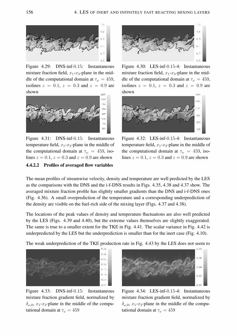
156 4. LES OF INERT AND INFINITELY FAST REACTING MIXING LAYERS
Figure 4.29: DNS-inf-0.15: Instantaneousmixture fraction field, x1-x3-plane in the mid-dle of the computational domain at τω = 459,isolines z = 0.1, z = 0.3 and z = 0.9 areshown
Figure 4.30: LES-inf-0.15-4: Instantaneousmixture fraction field, x1-x3-plane in the mid-dle of the computational domain at τω = 459,isolines z = 0.1, z = 0.3 and z = 0.9 areshown
Figure 4.31: DNS-inf-0.15: Instantaneoustemperature field, x1-x3-plane in the middle ofthe computational domain at τω = 459, iso-lines z = 0.1, z = 0.3 and z = 0.9 are shown
Figure 4.32: LES-inf-0.15-4: Instantaneoustemperature field, x1-x3-plane in the middle ofthe computational domain at τω = 459, iso-lines z = 0.1, z = 0.3 and z = 0.9 are shown
4.4.2.2 Profiles of averaged flow variables
The mean profiles of streamwise velocity, density and temperature are well predicted by the LESas the comparisons with the DNS and the i-f-DNS results in Figs. 4.35, 4.38 and 4.37 show. Theaveraged mixture fraction profile has slightly smaller gradients than the DNS and i-f-DNS ones(Fig. 4.36). A small overprediction of the temperature and a corresponding underprediction ofthe density are visible on the fuel-rich side of the mixing layer (Figs. 4.37 and 4.38).
The locations of the peak values of density and temperature fluctuations are also well predictedby the LES (Figs. 4.39 and 4.40), but the extreme values themselves are slightly exaggerated.The same is true to a smaller extent for the TKE in Fig. 4.41. The scalar variance in Fig. 4.42 isunderpredicted by the LES but the underprediction is smaller than for the inert case (Fig. 4.10).
The weak underprediction of the TKE production rate in Fig. 4.43 by the LES does not seem to
Figure 4.33: DNS-inf-0.15: Instantaneousmixture fraction gradient field, normalized byδω,0, x1-x3-plane in the middle of the compu-tational domain at τω = 459
Figure 4.34: LES-inf-0.15-4: Instantaneousmixture fraction gradient field, normalized byδω,0, x1-x3-plane in the middle of the compu-tational domain at τω = 459
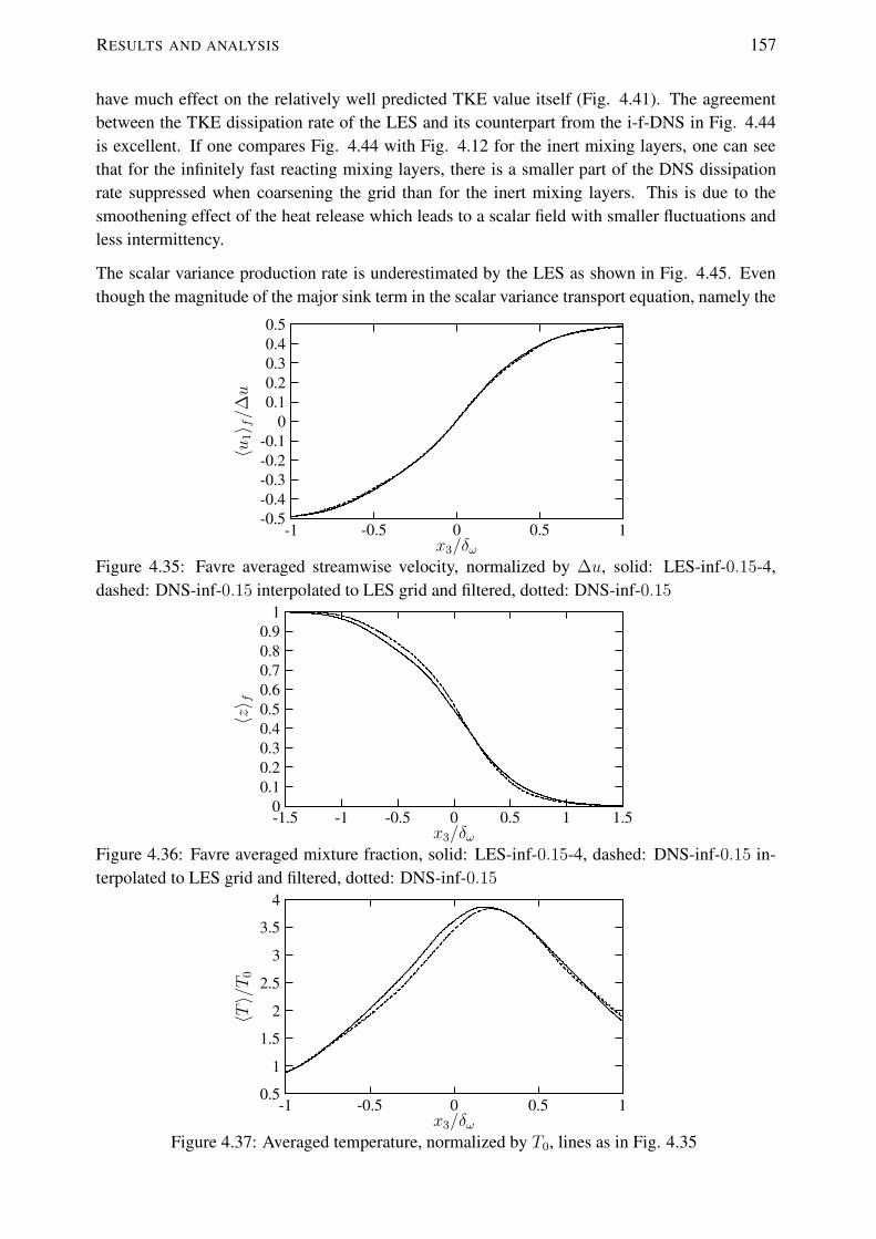
RESULTS AND ANALYSIS 157
have much effect on the relatively well predicted TKE value itself (Fig. 4.41). The agreementbetween the TKE dissipation rate of the LES and its counterpart from the i-f-DNS in Fig. 4.44is excellent. If one compares Fig. 4.44 with Fig. 4.12 for the inert mixing layers, one can seethat for the infinitely fast reacting mixing layers, there is a smaller part of the DNS dissipationrate suppressed when coarsening the grid than for the inert mixing layers. This is due to thesmoothening effect of the heat release which leads to a scalar field with smaller fluctuations andless intermittency.
The scalar variance production rate is underestimated by the LES as shown in Fig. 4.45. Eventhough the magnitude of the major sink term in the scalar variance transport equation, namely the
x3/δω
〈u1〉 f/∆
u
10.50-0.5-1
0.50.40.30.20.1
0-0.1-0.2-0.3-0.4-0.5
Figure 4.35: Favre averaged streamwise velocity, normalized by ∆u, solid: LES-inf-0.15-4,dashed: DNS-inf-0.15 interpolated to LES grid and filtered, dotted: DNS-inf-0.15
x3/δω
〈z〉 f
1.510.50-0.5-1-1.5
10.90.80.70.60.50.40.30.20.1
0
Figure 4.36: Favre averaged mixture fraction, solid: LES-inf-0.15-4, dashed: DNS-inf-0.15 in-terpolated to LES grid and filtered, dotted: DNS-inf-0.15
x3/δω
〈T〉/T
0
10.50-0.5-1
4
3.5
3
2.5
2
1.5
1
0.5
Figure 4.37: Averaged temperature, normalized by T0, lines as in Fig. 4.35

158 4. LES OF INERT AND INFINITELY FAST REACTING MIXING LAYERS
x3/δω
〈ρ〉/ρ
0
10.50-0.5-1
0.9
0.8
0.7
0.6
0.5
0.4
0.3
0.2
Figure 4.38: Averaged density, normalized by ρ0, lines as in Fig. 4.35
x3/δω
ρrms/〈ρ〉
10.50-0.5-1
0.55
0.5
0.45
0.4
0.35
0.3
0.25
0.2
Figure 4.39: Rms value of the density fluctuations, normalized by 〈ρ〉, lines as in Fig. 4.35
x3/δω
Trms/〈T〉
10.50-0.5-1
0.6
0.55
0.5
0.45
0.4
0.35
0.3
0.25
0.2
Figure 4.40: Rms value of the temperature fluctuations, normalized by 〈T 〉, lines as in Fig. 4.35
scalar dissipation rate in Fig. 4.46, is also underestimated, both effects lead to a too small scalarvariance. A refinement of the grid alleviates the problem partially and reduces the differencebetween LES and i-f-DNS (cf. Sect. 4.4.2.6).
4.4.2.3 The filtered heat release term
In this section, the modeling of the filtered heat release term by Eq. (4.25) is tested using a prioriand a posteriori procedures. For the a priori tests, the DNS fields are interpolated onto the LESgrid and filtered with a tophat filter. Then the terms in Eq. (4.25) are computed, whereby eitherthe exact values or the models (cf. Sects. 4.2.4.1 and 4.2.4.3) for (z2)sg and χ are used. Averagingover the homogeneous directions as well as the self-similar state and comparing the exact profiles

RESULTS AND ANALYSIS 159
x3/δω
k/∆
u2
10.50-0.5-1
0.035
0.03
0.025
0.02
0.015
0.01
0.005
0
Figure 4.41: Turbulent kinetic energy, normal-ized by ∆u2, lines as in Fig. 4.35
x3/δω
〈z′′2〉 f
10.50-0.5-1
0.050.045
0.040.035
0.030.025
0.020.015
0.010.005
0
Figure 4.42: Variance of mixture fraction,lines as in Fig. 4.35
x3/δω
Pδ ω/
(ρ0∆u
3)
10.50-0.5-1
0.003
0.0025
0.002
0.0015
0.001
0.0005
0
-0.0005
Figure 4.43: Production of TKE, normalizedby δω/ (ρ0∆u3), lines as in Fig. 4.35
x3/δω
Dδ ω/
(ρ0∆u
3)
10.50-0.5-1
0-0.0002-0.0004-0.0006-0.0008
-0.001-0.0012-0.0014-0.0016-0.0018
-0.002
Figure 4.44: Dissipation rate of TKE, normal-ized by δω/ (ρ0∆u3), lines as in Fig. 4.35
x3/δω
Pzδ ω/
(ρ0∆u
)
10.50-0.5-1
0.0035
0.003
0.0025
0.002
0.0015
0.001
0.0005
0
Figure 4.45: Production terms of thescalar variance transport equation,Pz = −〈ρz′′u′′3〉∂〈z〉f∂x3
− 12〈ρz′′2〉∂〈u3〉f
∂x3,
normalized by δω/ (ρ0∆u), lines as in Fig.4.35
x3/δω
ε zδ ω/
(ρ0∆u
)
10.50-0.5-1
0-0.0002-0.0004-0.0006-0.0008
-0.001-0.0012-0.0014-0.0016-0.0018
-0.002
Figure 4.46: Scalar dissipation rate, εz =
−〈 µSc
∂z∂xj
∂z∂xj〉, lines as in Fig. 4.35
of (z2)sg and χ with the modeled ones, allows an optimal adaption of the model coefficients CGRz
and CGRχ .
The first modeled quantity that the heat release term depends on is the subgrid scalar variance(z2)sg which enters the beta-pdf. Figure 4.47 shows three profiles: the exact profile computed byEq. (4.29) from interpolated and filtered DNS data, the profile that results when using gradientmodel, Eq. (4.30), a priori (i.e. with the exact gradient from the interpolated and filtered DNSdata) and, finally, the a posteriori profile from the LES. The agreement between (z2)sg from theLES and the corresponding value of the gradient model computed from DNS data is good forboth, the peak value and the shape. The peak value is already well predicted in the a priori testwhich is due to the adaption of the model coefficient. Concerning the shape of the (z2)sg profile,in particular on the fuel-rich side, the a posteriori test performs even better.
The model of the filtered heat release term depends on the beta-pdf via the factor I , Eq. (4.38).Figure 4.48 shows a comparison between its exact profile and the a priori and a posteriori values.Besides (z2)sg, the filtered value z enters into the computation of I . Even though the averagedLES fields of both (z2)sg (Fig. 4.47 ) and z (LES curve in Fig. 4.36) agree quite well with the

160 4. LES OF INERT AND INFINITELY FAST REACTING MIXING LAYERS
x3/δω
〈(z2) sg〉
1.510.50-0.5-1-1.5
0.00450.004
0.00350.003
0.00250.002
0.00150.001
0.00050
Figure 4.47: Subgrid scalar variance, solid: LES-inf-0.15-4, dashed: a priori test of model withdata from DNS-inf-0.15, dotted: exact value from DNS-inf-0.15
x3/δω
〈I〉
1.510.50-0.5-1-1.5
1.61.41.2
10.80.60.40.2
0-0.2
Figure 4.48: Integral I , lines as in Fig. 4.47
x3/δω
〈χ〉δω/∆
u
1.510.50-0.5-1-1.5
0.008
0.007
0.006
0.005
0.004
0.003
0.002
0.001
0
Figure 4.49: Filtered scalar dissipation rate, normalized by ∆u/δω, lines as in Fig. 4.47
DNS results, there must be differences in the higher moments of the mixture fraction betweenLES and DNS as the overestimation of I suggests. The a priori test of I , however, is excellent.
The model of the filtered scalar dissipation rate is given by Eq. (4.44). A comparison of theexact averaged value of χ with the a priori and a posteriori determined ones is shown in Fig.4.49. Again, the model coefficient in Eq. (4.44) has been adapted such that the a priori testgives the best possible approximation of the exact χ. About 50 % of χ are from its subgrid partχsg = χ−χls with χls from Eq. (4.40). This is shown in Fig. 4.50 . The figure also demonstratesthat the overestimation of χ by the LES (Fig. 4.49 ) is mainly due to an overestimation of itssubgrid part modeled by the gradient model.

RESULTS AND ANALYSIS 161
x3/δω
〈χsg〉δω/∆
u
1.510.50-0.5-1-1.5
0.004
0.0035
0.003
0.0025
0.002
0.0015
0.001
0.0005
0
Figure 4.50: Subgrid part of scalar dissipation rate, normalized by ∆u/δω, lines as in Fig. 4.47
x3/δω
〈Qe〉/
∆u
2
1.510.50-0.5-1-1.5
580
575
570
565
560
555
Figure 4.51: Heat release parameter Qe, normalized by ∆u2, solid: LES-inf-0.15-4, dashed: datafrom DNS-inf-0.15
x3/δω
〈ω〉δω/
(ρ0∆u
3)
1.510.50-0.5-1-1.5
21.81.61.41.2
10.80.60.40.2
0-0.2
Figure 4.52: Filtered source term ω, normalized by ρ0∆u3/δω, lines as in Fig. 4.47
Since the remaining factor in the expression for ω, the heat release parameter Qe (Eq. (4.26)) iswell predicted by the LES, the overestimation of the heat release term itself (Fig. 4.52) can bemainly traced back to the overestimations of I and χ. However, the a priori computed sourceterm ω also overestimates the actual value. This leads to the conclusion that correlations betweenthe factors in Eq. (4.25) play a role. The overestimation of ω, nevertheless, can be consideredas tolerable when taking into account the good results for the averaged density and temperatureprofiles (Figs. 4.38 and 4.37).
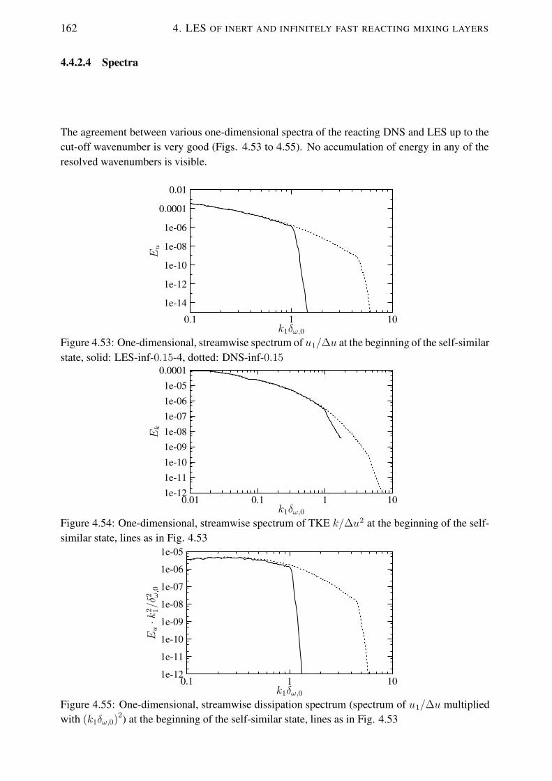
162 4. LES OF INERT AND INFINITELY FAST REACTING MIXING LAYERS
4.4.2.4 Spectra
The agreement between various one-dimensional spectra of the reacting DNS and LES up to thecut-off wavenumber is very good (Figs. 4.53 to 4.55). No accumulation of energy in any of theresolved wavenumbers is visible.
k1δω,0
Eu
1010.1
0.01
0.0001
1e-06
1e-08
1e-10
1e-12
1e-14
Figure 4.53: One-dimensional, streamwise spectrum of u1/∆u at the beginning of the self-similarstate, solid: LES-inf-0.15-4, dotted: DNS-inf-0.15
k1δω,0
Ek
1010.10.01
0.0001
1e-05
1e-06
1e-07
1e-08
1e-09
1e-10
1e-11
1e-12
Figure 4.54: One-dimensional, streamwise spectrum of TKE k/∆u2 at the beginning of the self-similar state, lines as in Fig. 4.53
k1δω,0
Eu·k
2 1/δ
2 ω,0
1010.1
1e-05
1e-06
1e-07
1e-08
1e-09
1e-10
1e-11
1e-12
Figure 4.55: One-dimensional, streamwise dissipation spectrum (spectrum of u1/∆u multipliedwith (k1δω,0)2) at the beginning of the self-similar state, lines as in Fig. 4.53

RESULTS AND ANALYSIS 163
4.4.2.5 Effect of filtering on dissipation rates
In a procedure analogous to that for inert mixing layers in Sect. 4.4.1.4, instantaneous filterdissipation and scalar dissipation rates at the beginning of the self-similar state are computed forthe reacting mixing layers. The results, as well as the actual scalar dissipation rates derived fromLES and DNS data, are shown in Figs. 4.58 and 4.59. Added together, the filter dissipation rateand the LES TKE dissipation rate in Fig. 4.58 equate approximately the TKE dissipation rate ofthe DNS. The same is true for the scalar dissipation rates in Fig. 4.59.
4.4.2.6 Refinement of the grid
Quantities which were not perfectly captured by the LES when coarsening the DNS grid by factorfour in each direction are better approximated when coarsening the DNS grid by factor two ineach direction only. Two examples are shown in Figs. 4.60 and 4.61: The variance of the mixturefraction and the mean heat release term (compare with Figs. 4.42 and 4.61). For the latter one, weobserve that the a priori computed profile and the a posteriori computed one collapse while theactual profile computed without any models from DNS results is below these curves. This leadsto the conclusion that the remaining differences between LES and DNS concerning the profile ofω are mainly due to correlations between the single factors in Eq. (4.25) since the a posteriori
k1δω,0
Ez
1010.10.01
0.01
0.001
0.0001
1e-05
1e-06
1e-07
1e-08
1e-09
Figure 4.56: One-dimensional, streamwise spectrum of the mixture fraction z at the beginning ofthe self-similar state, lines as in Fig. 4.53
k1δω,0
Ez·k
2 1/δ
2 ω,0
1010.1
0.0001
1e-05
1e-06
1e-07
1e-08
1e-09
1e-10
Figure 4.57: One-dimensional dissipation spectrum of the mixture fraction z (spectrum of zmultiplied with (k1δω,0)2) at the beginning of the self-similar state, lines as in Fig. 4.53
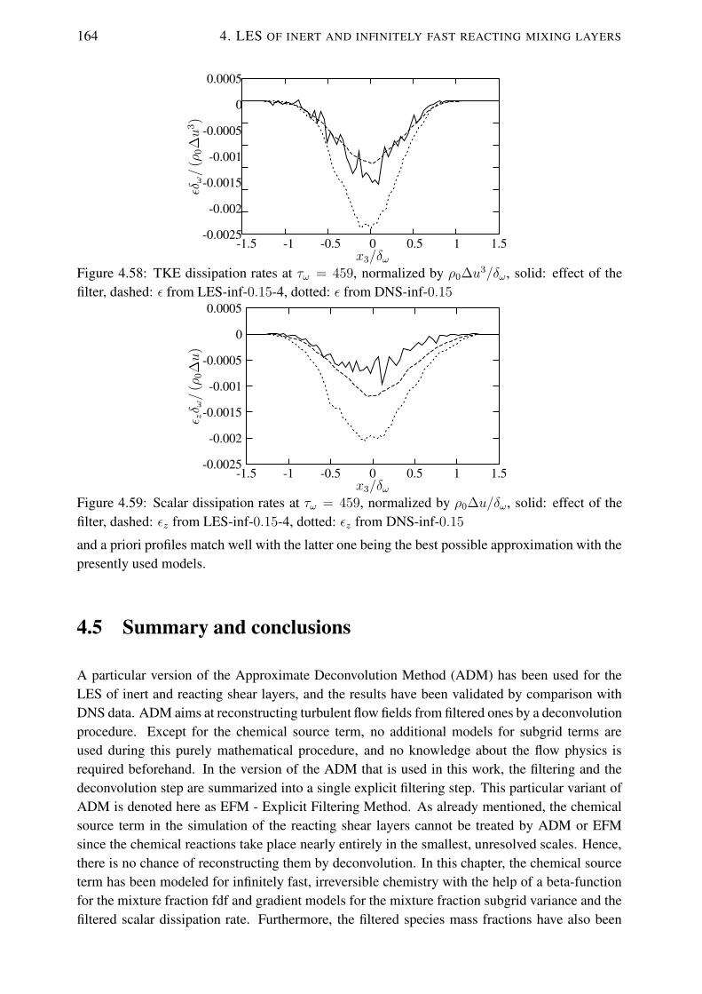
164 4. LES OF INERT AND INFINITELY FAST REACTING MIXING LAYERS
x3/δω
εδω/
(ρ0∆u
3)
1.510.50-0.5-1-1.5
0.0005
0
-0.0005
-0.001
-0.0015
-0.002
-0.0025
Figure 4.58: TKE dissipation rates at τω = 459, normalized by ρ0∆u3/δω, solid: effect of thefilter, dashed: ε from LES-inf-0.15-4, dotted: ε from DNS-inf-0.15
x3/δω
ε zδ ω/
(ρ0∆u
)
1.510.50-0.5-1-1.5
0.0005
0
-0.0005
-0.001
-0.0015
-0.002
-0.0025
Figure 4.59: Scalar dissipation rates at τω = 459, normalized by ρ0∆u/δω, solid: effect of thefilter, dashed: εz from LES-inf-0.15-4, dotted: εz from DNS-inf-0.15
and a priori profiles match well with the latter one being the best possible approximation with thepresently used models.
4.5 Summary and conclusions
A particular version of the Approximate Deconvolution Method (ADM) has been used for theLES of inert and reacting shear layers, and the results have been validated by comparison withDNS data. ADM aims at reconstructing turbulent flow fields from filtered ones by a deconvolutionprocedure. Except for the chemical source term, no additional models for subgrid terms areused during this purely mathematical procedure, and no knowledge about the flow physics isrequired beforehand. In the version of the ADM that is used in this work, the filtering and thedeconvolution step are summarized into a single explicit filtering step. This particular variant ofADM is denoted here as EFM - Explicit Filtering Method. As already mentioned, the chemicalsource term in the simulation of the reacting shear layers cannot be treated by ADM or EFMsince the chemical reactions take place nearly entirely in the smallest, unresolved scales. Hence,there is no chance of reconstructing them by deconvolution. In this chapter, the chemical sourceterm has been modeled for infinitely fast, irreversible chemistry with the help of a beta-functionfor the mixture fraction fdf and gradient models for the mixture fraction subgrid variance and thefiltered scalar dissipation rate. Furthermore, the filtered species mass fractions have also been

SUMMARY AND CONCLUSIONS 165
x3/δω
〈z′′2〉 f
10.50-0.5-1
0.050.0450.04
0.0350.03
0.0250.02
0.0150.01
0.0050
Figure 4.60: Variance of mixture fraction, solid: LES-inf-0.15-2, dashed: DNS-inf-0.15 interpo-lated to LES grid and filtered, dotted: DNS-inf-0.15
x3/δω
〈ω〉δω/
(ρ0∆u
3)
1.510.50-0.5-1-1.5
1.81.61.41.2
10.80.60.40.2
0-0.2
Figure 4.61: Mean filtered heat release term ω, normalized by ρ0∆u3/δω, solid: LES-inf-0.15-4,dashed: a priori test of model with data from DNS-inf-0.15, dotted: exact value from DNS-inf-0.15
obtained by integration with a beta-fdf for the mixture fraction. Coefficients for the models havebeen adapted in a priori tests using DNS data.
The LES performed and analyzed are temporally evolving, turbulent mixing layers at Mc = 0.15,inert and infinitely fast reacting. They have been initialized well before the attainment of the self-similar state from corresponding DNS flow fields that had been interpolated to the coarser LESgrid and filtered. Two different resolutions for the LES have been used: One with 8 times less gridpoints than the DNS and one with 64 times less grid points. A further coarsening of the grid wouldalso be possible if only stability was the criteria for a successful LES and less quality of the resultswas allowed. This concerns in particular quantities that are dominated by small scales like theTKE dissipation rate and the scalar dissipation rate. However, computation on a grid as coarseas possible is not the goal of the present work, and we have opted for a compromise betweencomputational effort and good results by chosing relatively fine LES grids. Statistics from theLES data were taken over the self-similar states of the mixing layers and compared to DNS dataas well as DNS data that had been interpolated to the LES grid and filtered. A comparison ofinstantaneous scalar (mass and mixture fractions) and scalar gradient distributions have revealedthat, while large structures have been successfully captured by the LES, this, as expected, has notbeen the case for small structures, and the LES fields appear consequently more ’blurred’. Thisis particularly strong for the intermittent scalar gradients, the highest values of which are situatedin the smallest scales, that cannot be resolved in an LES.

166 4. LES OF INERT AND INFINITELY FAST REACTING MIXING LAYERS
For the inert mixing layers, an excellent capturing of flow dynamical quantities like the meanstreamwise velocity and the turbulent kinetic energy (TKE) is observed, even for the resolutionwith 64 times less grid points than the DNS. Moreover, the most important terms in the TKEtransport equation, namely production and the dissipation rates, are reproduced well, with a goodagreement of the LES profiles and the profiles from the interpolated DNS data. The same istrue for the pressure-strain correlations steering the re-distribution of energy from the streamwiseReynolds stress component to the spanwise and transverse ones. The one-dimensional spectra ofthe streamwise velocity, the turbulent kinetic energy and the dissipation rate show the expectedbehaviour: The LES spectra follow the DNS spectra up to the cut-off frequency, and no spuriousaccumulation of energy is visible in the highest resolved wavenumbers. However, a good captur-ing of scalar-related quantities seems to be more difficult, even for the inert mixing layers: Toosmall amplitudes of the LES profile compared to the filtered DNS profile for the mass fractionvariances and their production rates have been observed. The one-dimensional scalar and scalardissipation spectra show a slight accumulation of energy in the highest resolved wavenumbers.These difficulties are traced back to the fact that the scalar field is more sensitive to the smallscales than the velocity field which complicates its modeling. However, the simulations with thefiner grid (8 times less grid points than the DNS) show a significant improvement of the results.
For the LES of the reacting mixing layers, not only an excellent capturing of flow dynamicalquantities (mean velocity, TKE), but also of thermodynamical quantities (mean temperature anddensity and the corresponding rms values) has been observed, even for the coarsest resolution thathas been investigated. As for the inert mixing layers, scalar-related quantities, like the varianceof the mixture fraction show discrepancies between the LES and the interpolated DNS profilesthat are, however, reduced by a refinement of the LES grid. A priori and a posteriori tests of thefiltered heat release term have also been performed. Its weak overestimation by LES has been ledback to a slight overestimation of the subgrid scalar dissipation rate by the Smagorinsky modeland to differences between LES and filtered DNS in higher moments of the mixture fraction.These deficiencies have been reduced when refining the LES grid. The mixture fraction subgridvariance has been captured excellently by the gradient model, even at the coarser resolution.Since the spectra for the reacting mixing layers are less dominated by the small scales than theinert ones, they are easier to reproduce (up to the cut-off frequency) by the LES, and no spuriousaccumulation of energy has been observed in the highest resolved wavenumbers, neither in theone-dimensional spectra for the streamwise velocity, the TKE and its dissipation rate, nor in thespectra for the scalar and the scalar dissipation rate.
Finally, it can be concluded that EFM (combined with proper heat release modeling for reactingflow) has been proven to be a successful and efficient LES model for inert and infinitely fastreacting turbulent mixing layers. As for any LES model, it is necessary to make compromisesbetween the quality of the results and computational effort.
Even though only results for Mc = 0.15 have been shown in the present chapter, also inert andreacting shear layers at higher convective Mach numbers have been simulated successfully withEFM. However, since the following chapter deals with reacting mixing layers at the same lowMach number and shows an extension of the combustion model to include finite-rate chemistryand detailed diffusion, it has been decided not to extend the analysis of the present chapter tohigher Mach numbers.

5 LES of shear layers with chemical ki-netic and detailed diffusion effects
5.1 Introduction and literature survey
While in the previous chapters DNS and LES of reacting mixing layers with infinitely fast chem-istry and simplified diffusion have been performed, the aim of this chapter is to take into accountchemical kinetic and detailed diffusion effects by using an LES flamelet model. A classificationof flamelet approaches within the range of combustion models has been provided in Sect. 4.1.
Besides a simplified treatment of chemistry, many existing turbulent combustion models alsouse simplified diffusion processes [73]. Multicomponent and thermal diffusion effects are onlyincluded in recent Direct Numerical Simulations (DNS) of turbulent combustion [40] and showmainly local influences on the flame structure. To our knowledge, only one attempt has beenmade to include these effects in a flamelet model for a Large Eddy Simulation (LES) [131]. Inthe present chapter, the formulation of the flamelet equations in physical space as well as thedefinition of the mixture fraction and its diffusivity is the same as in the work of Pierce & Moin[131], but the LES model is different. While Pierce & Moin apply eddy diffusivity and eddyviscosity models with dynamically evaluated coefficients, the LES model used in this work is amodified version of the approximate deconvolution method (ADM) [175, 176] and has alreadybeen presented in the previous chapter. In [131], Pierce & Moin mention the possibility to includedifferent diffusion models in their flamelet model and show some LES results for a methane-fuelled coaxial jet combustor with different diffusion approximations. Based on these results, theyargue that an accurate treatment of mass diffusion can be just as important as accurate modelingof chemical kinetics. The fact that the authors do not pursue the issue further, but concentrateinstead on the advantages of a progress variable to capture unsteady, lifted flame dynamics [132],is one of the motivations to investigate detailed diffusion effects in the present work.
Most authors who considered effects of detailed diffusion in flamelets and laminar diffusionflames concentrated mainly on two species with different but constant diffusivities or Lewis num-bers [34, 119] or neglected thermal diffusion [138]. Therefore, almost no data is available com-paring different levels of approximation for the species diffusion fluxes and the heat flux withrespect to multicomponent, Soret and Dufour effects. One aim of the present chapter is to seetheir influence in a basic configuration for non-premixed hydrogen combustion, namely a tempo-rally evolving turbulent shear layer.
This chapter is organized as follows: Section 5.2 explains the essential features of the LES witha particular focus on the modeling of the filtered heat release term and the filtered species massfractions. The computation and tabulation of the steady flamelets is dealt with in Sect. 5.3. It isalso explained how the detailed chemistry is implemented and what different approximations ofthe diffusion fluxes and the heat flux vector are used. In Section 5.4, configuration, initialization

168 5. LES OF SHEAR LAYERS WITH CHEMICAL KINETIC AND DETAILED DIFFUSION EFFECTS
and essential parameters of the mixing layer LES are presented and related to the ones of test casesfrom other chapters of this work. Section 5.5 is dedicated to the results and their analysis: First,laminar flamelets with different diffusion approximations are compared with each other (Sect.5.5.1). Then, the LES results are validated by comparison with DNS data (Sect. 5.5.2). Moreover,the differences between the LES results with detailed and simplified diffusion are assessed andcontrasted with those encountered between the respective laminar flamelets. Conclusions aredrawn in Sect. 5.6.
5.2 LES approach
5.2.1 LES equations and models
During the LES, the compressible transport equations for the pressure p, the Cartesian velocitycomponents ui, the temperature T and a passive scalar, which is the mixture fraction z, are in-tegrated by using sixth-order compact central schemes for the spatial derivatives in all directionsand a third order low-storage Runge-Kutta scheme for time integration. The transport equationsfor p, ui and T are the same as given in Eq. (4.16). In the transport equation of z, the diffusivityof the mixture fraction, αz, is used:
∂z
∂t= −ui
∂z
∂xi+
1
ρ
∂
∂xi
(αzρ
∂z
∂xi
)(5.1)
αz depends on elemental diffusive fluxes and is therefore not constant. Its determination is ex-plained in Sect. 5.3.3.
After each time integration step, an explicit filtering step (with the composite (Q ∗G)2 filter) ofthe primitive flow variables as described in Sect. 4.2.1 is performed. This procedure implicitlymodels the subgrid terms arising from non-linearities when low-pass filtering and projecting thetransport equations onto a coarse LES grid. Only the filtered heat release term
ω = −∑
α
hαωα (5.2)
which appears in the transport equations of the pressure and the temperature has to be modeledseparately. In Sect. 5.2.2, it is explained how this is done for finite-rate chemistry using a flameletdatabase.
Two additional quantities have to be modeled during the LES, since they are required for theretrieval of the filtered chemical source term and the filtered species mass fractions from theflamelet database (cf. Sect. 5.3): the subgrid variance of the mixture fraction,
(z2)sg
= z2 − z2 (5.3)
and the filtered scalar dissipation rate,
χ =˜
αz
(∂z
∂xi
)2
. (5.4)
Both quantities, (z2)sg and χ, are computed with gradient models which are given by Eqs. (4.30)and (4.44).
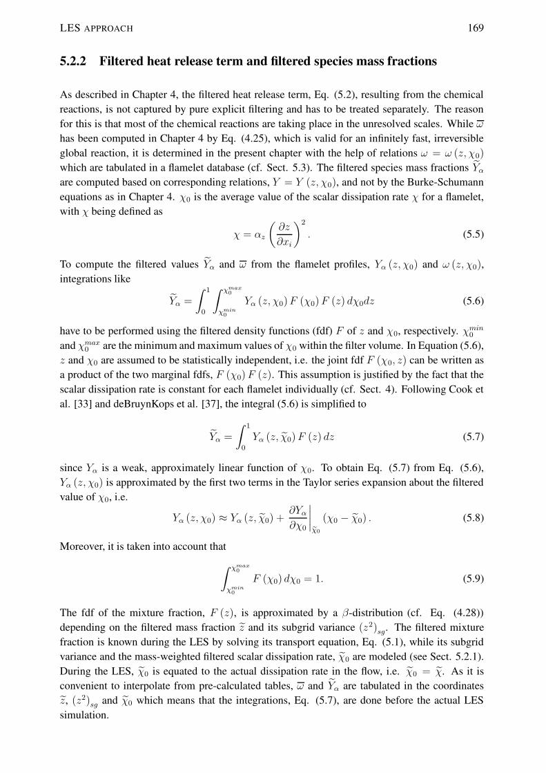
LES APPROACH 169
5.2.2 Filtered heat release term and filtered species mass fractions
As described in Chapter 4, the filtered heat release term, Eq. (5.2), resulting from the chemicalreactions, is not captured by pure explicit filtering and has to be treated separately. The reasonfor this is that most of the chemical reactions are taking place in the unresolved scales. While ωhas been computed in Chapter 4 by Eq. (4.25), which is valid for an infinitely fast, irreversibleglobal reaction, it is determined in the present chapter with the help of relations ω = ω (z, χ0)
which are tabulated in a flamelet database (cf. Sect. 5.3). The filtered species mass fractions Yαare computed based on corresponding relations, Y = Y (z, χ0), and not by the Burke-Schumannequations as in Chapter 4. χ0 is the average value of the scalar dissipation rate χ for a flamelet,with χ being defined as
χ = αz
(∂z
∂xi
)2
. (5.5)
To compute the filtered values Yα and ω from the flamelet profiles, Yα (z, χ0) and ω (z, χ0),integrations like
Yα =
∫ 1
0
∫ χmax0
χmin0
Yα (z, χ0)F (χ0)F (z) dχ0dz (5.6)
have to be performed using the filtered density functions (fdf) F of z and χ0, respectively. χmin0
and χmax0 are the minimum and maximum values of χ0 within the filter volume. In Equation (5.6),z and χ0 are assumed to be statistically independent, i.e. the joint fdf F (χ0, z) can be written asa product of the two marginal fdfs, F (χ0)F (z). This assumption is justified by the fact that thescalar dissipation rate is constant for each flamelet individually (cf. Sect. 4). Following Cook etal. [33] and deBruynKops et al. [37], the integral (5.6) is simplified to
Yα =
∫ 1
0
Yα (z, χ0)F (z) dz (5.7)
since Yα is a weak, approximately linear function of χ0. To obtain Eq. (5.7) from Eq. (5.6),Yα (z, χ0) is approximated by the first two terms in the Taylor series expansion about the filteredvalue of χ0, i.e.
Yα (z, χ0) ≈ Yα (z, χ0) +∂Yα∂χ0
∣∣∣∣eχ0
(χ0 − χ0) . (5.8)
Moreover, it is taken into account that
∫ χmax0
χmin0
F (χ0) dχ0 = 1. (5.9)
The fdf of the mixture fraction, F (z), is approximated by a β-distribution (cf. Eq. (4.28))depending on the filtered mass fraction z and its subgrid variance (z2)sg. The filtered mixturefraction is known during the LES by solving its transport equation, Eq. (5.1), while its subgridvariance and the mass-weighted filtered scalar dissipation rate, χ0 are modeled (see Sect. 5.2.1).During the LES, χ0 is equated to the actual dissipation rate in the flow, i.e. χ0 = χ. As it isconvenient to interpolate from pre-calculated tables, ω and Yα are tabulated in the coordinatesz, (z2)sg and χ0 which means that the integrations, Eq. (5.7), are done before the actual LESsimulation.

170 5. LES OF SHEAR LAYERS WITH CHEMICAL KINETIC AND DETAILED DIFFUSION EFFECTS
5.3 The flamelet database
Instead of computing the 1D flamelets in mixture fraction space [33, 128], they are computed inphysical space (coordinate x) with zero velocity [131, 132]. Assuming constant pressure, which isjustified by the low Mach number in the DNS and LES computations, the following 1D transportequations are obtained from the complete conservation equations for temperature, species massfractions and a passive scalar:
∂T
∂t=
1
ρcv
[−∂qx∂x−∑
α
(hα −
RWα
T
)(−∂ρY Vαx
∂x+ ωα
)](5.10)
∂Yα∂t
=1
ρ
(− ∂
∂x(ρYαVαx) + ωα
)(5.11)
∂z
∂t=
1
ρ
∂
∂x
(αzρ
∂z
∂x
)(5.12)
The passive scalar z is the mixture fraction. Solving transport equations for this quantity and thespecies mass fractions, Yα, simultaneously, allows to establish relations between z and Yα whichare later used for the tabulation of the flamelets. An alternative to solving the transport equationof z would be to compute z by its definition based on species mass fractions (see below: Eqs.(5.26) and (5.27)). However, as Pierce & Moin (2001) emphasize, this approach is equivalent tointegrating Eq. (5.12) with an initial mixture fraction distribution given by Eq. (5.27).
The species diffusion flux YαVαx and the heat flux vector qx in Eqs. (5.10) and (5.11) are evaluatedas described in Sect. 5.3.2. either with detailed or with simplified diffusion.
The computation of the mixture fraction diffusivity, αz is further detailed in Sect. 5.3.3.
5.3.1 Detailed reaction scheme and Arrhenius chemistry
The chemical production rates ωα in Eqs. (5.10) and (5.11) are computed with full Arrheniuschemistry using the reaction scheme of Miller et al. [113] that is given in table 5.1. It involves9 species, O2, H2, H2O, N2, O, H , OH , H2O2 and HO2 and 19 elemental reactions. The samereaction scheme has been used by de Charantenay & Ern [40] for various premixed 2D H2/O2
flames with detailed diffusion.
Each elementary reaction in Table 5.1 can be written in the form∑
α
ν ′α,irctSα ↔∑
α
ν ′′α,irctSα (5.13)
with Sα denoting the chemical symbol of species α. For each reaction irct, mass conservationcan be written with the help of the stoichiometric coefficients of the forward reaction, ν ′α,irct, andof the backward reaction, ν ′′α,irct:
∑
α
ν ′α,irctWα =∑
α
ν ′′α,irctWα (5.14)

THE FLAMELET DATABASE 171
This can also be written as ∑
α
να,irctWα = 0 (5.15)
with να,irct = ν ′α,irct − ν ′′α,irct. The mass reaction rate of species α that appears in Eqs. (5.10) and(5.11) is given by
ωα = Wα
∑
irct
να,irctwirct. (5.16)
It is the sum of contributions from the elementary reactions with the progress rates wirct,
wirct = kf,irctΠαCν′α,irctα − kb,irctΠαC
ν′′α,irctα . (5.17)
The molar concentration of species α is denoted by Cα = ρYα/Wα and the forward and backwardconstants of reaction irct by kf,irct and kb,irct. The forward constant of each elementary reactionis computed with the help of a semi-empirical Arrhenius law in the form
kf,irct = AirctTβirct exp
(−EirctRT
). (5.18)
Table 5.1: Reaction scheme for H2/O2 combustion with pre-exponential factors A, temperature-dependence coefficients β and activation energies E [113]
Reaction A in (cm,mol, s) β E in cal/mol
(1) H2 +O2 ↔ 2OH 1.70 · 1013 0.00 47780
(2) H2 +OH ↔ H2O +H 1.17 · 109 1.30 3626
(3) H +O2 ↔ OH +O 2.00 · 1014 0.00 16800
(4) O +H2 ↔ OH +H 1.80 · 1010 1.00 8826
(5) H +O2 +M ↔ HO2 +M 2.10 · 1018 −1.00 0
H2O/21/H2/3.3/O2/0.0/N2/0.0
(6) H +O2 +O2 ↔ HO2 +O2 6.70 · 1019 −1.42 0
(7) H +O2 +N2 ↔ HO2 +N2 6.70 · 1019 −1.42 0
(8) OH +HO2 ↔ H2O +O2 5.00 · 1013 0.00 1000
(9) H +HO2 ↔ 2OH 2.50 · 1014 0.00 1900
(10) O +HO2 ↔ O2 +OH 4.80 · 1013 0.00 1000
(11) 2OH ↔ O +H2O 6.00 · 108 1.30 0
(12) H2 +M ↔ H +H +M 2.23 · 1012 0.50 92600
H2O/6/H/2/H2/3
(13) O2 +M ↔ 2O +M 1.85 · 1011 0.50 95560
(14) H +OH +M ↔ H2O +M 7.50 · 1023 −2.60 0
H2O/20
(15) H +HO2 ↔ H2 +O2 2.50 · 1013 0.00 700
(16) HO2 +HO2 ↔ H2O2 +O2 2.00 · 1012 0.00 0
(17) H2O2 +M ↔ OH +OH +M 1.30 · 1017 0.00 45500
(18) H2O2 +H ↔ HO2 +H2 1.60 · 1012 0.00 3800
(19) H2O2 +OH ↔ H2O +HO2 1.00 · 1013 0.00 1800

172 5. LES OF SHEAR LAYERS WITH CHEMICAL KINETIC AND DETAILED DIFFUSION EFFECTS
Forward and backward coefficients of each reaction are linked by the equilibrium constantKe,irct,
Ke,irct =kf,irctkb,irct
, (5.19)
which is determined by [142]
Ke,irct =
(p0
RT
)Pα να,irct
exp
[∆S0
irct
R − ∆H0irct
RT
](5.20)
with the entropy and enthalpy changes, ∆S0irct and ∆H0
irct, during reaction irct at referencepressure p0 = 1013.25hPa. In some reactions, like in reaction (5) in Table 5.1, a third compounddenoted by M is involved. Elements present in the gas mixture act as such a third compound, theeffective concentration of which is computed by
CM,irct =∑
α
γα,irctCα. (5.21)
The pre-factors γα,irct are mostly 1. Exceptions are given in Table 5.1 in the second line of therespective reaction, e.g. γH2O,5 = 21. The progress of a reaction with a third compound involvedis computed by
wirct = CM,irct ·(kf,irctΠαC
ν′α,irctα − kb,irctΠαC
ν′′α,irctα
). (5.22)
5.3.2 Computation of detailed diffusion fluxes and of heat flux by EGlib
To establish the flamelet databases, detailed transport properties, and in particular the diffusionfluxes YαVαx and the heat flux qx, are evaluated with the help of subroutines from the library EGlib[54]. EGlib uses an iterative method to obtain an approximate solution for the linear equationsof the transport coefficients derived from kinetic theory. Truncation then provides, at a moderatecomputational cost, approximate expressions of desired accuracy for the transport coefficients.This is in contrast to the two ’traditional’ approaches for evaluating transport coefficients, namelythe direct numerical inversion of the linear equations, which is computationally expensive, andthe use of empirical average expressions. The latter often leads to poorly accurate transportcoefficients.
EGlib was first applied to laminar flames [55, 56], and it was shown that the accuracy of the trans-port coefficients severely influenced the flame properties. Later, de Charentenay and Ern [40] usedit for various premixed 2D H2/O2 flames and found local modifications of turbulent flame prop-erties by multicomponent transport that were much larger than those observed for laminar flames.In particular, the propagation velocity and the stretch in regions where the flame front experiencesstrong curvature effects were affected. Even though the impact on global flame properties wasshown to be only moderate because of the smoothening induced by turbulent fluctuations, theseauthors concluded that for some types of flames (highly curved or with quenching phenomena),multicomponent transport plays a sufficiently relevant role to be included in accurate simulations.
In this chapter, results of computations performed with the detailed diffusion description givenby Eqs. (2.8) to (2.10) are compared with those using a simplified description of diffusion andheat flux. In the simplified description, the thermodiffusive effects, namely the Soret and Dufour

THE FLAMELET DATABASE 173
effects, are neglected and the Hirschfelder-Curtiss approximation [74] for the species diffusioncoefficients in the mixture is used. The simplified diffusion flux vector reads (in 3D)
YαVαi = −∑
β
Dαβ,apprdβi (5.23)
with the approximate flux diffusion matrix based on the diffusion coefficient of species α in themixture, Dα,m:
Dα,m =
∑β 6=α Yβ∑
β 6=αXβ/Dαβ
. (5.24)
As each species has just one diffusion coefficient in the mixture, which depends of course onthe local conditions, namely temperature and species’ composition, no cross-diffusion effectsare taken into account. The use of Dα,m, which is computed with the help of EGlib [53, 55],corresponds to the so-called Hirschfelder-Curtiss approximation [74] of scalar diffusion.
The simplified description of the heat flux is
qi =∑
α
ρhαYαVαi − λ∂T
∂xi(5.25)
with the thermal conductivity λ, which is also given by EGlib.
5.3.3 The mixture fraction and its diffusivity
Following Pierce & Moin [131, 132], the mixture fraction z is defined as an average mass fractionby combining the conserved elemental (atomic) mass fractions. The elemental mass fractions aγare given by
aγ =∑
α
YαNαγAγ/Wα, (5.26)
where Nαγ is the number of γ atoms in each molecule of species α. Aγ are atomic weights andWα molecular weights. After summing the elemental mass fractions and normalizing the result,the average mixture fraction is given by
z =
∑γ |aγ − aγ1|∑γ |aγ2 − aγ1|
, (5.27)
where aγ1 and aγ2 are the elemental mass fractions in the oxidizer and fuel streams, respectively.Elemental diffusive fluxes aγx can be combined by
aγx =∑
α
ρYαVαxNαγAγ/Wα. (5.28)
Finally, αz is computed from
ραz
∣∣∣∣∂z
∂x
∣∣∣∣ =
∑γ |aγx|∑
γ |aγ2 − aγ1|. (5.29)
An analogous 3D expression, which is used to compute αz during the LES, is easily obtainedfrom Eq. (5.29).

174 5. LES OF SHEAR LAYERS WITH CHEMICAL KINETIC AND DETAILED DIFFUSION EFFECTS
The particular definition of the mixture fraction by Eq. (5.27), which is not only used for comput-ing the flamelet database but also in the LES, is one feature that distinguishes the present flameletcomputations from others, for example from Pitsch & Peters [138], where the mixture fraction isnot related directly to any combination of the reactive scalars, but defined from the solution of aconservation equation with an arbitrary diffusion coefficient Dz and appropriate boundary condi-tions. Even though this approach allows to incorporate detailed diffusion effects into the flameletdatabase, while maintaining consistency in the mixture fraction evolution equation, it relies on theassumption that there exists a mixture fraction that is a conserved scalar and eliminates detaileddiffusion by having the diffusion coefficient Dz. That the existence of such a mixture fractionis questionable has been shown for example by Sutherland [179]. Quantifications of detaileddiffusion in experiments of turbulent, non-premixed jet flames of H2 and CO2 [170] were alsoperformed with the help of elemental mixture fractions, the definition of which uses elementalmass fractions similar to Eq. (5.27), but with one particular element, the mixture fraction is basedon. Other types of elemental mixture fractions were used for example by [5, 11]. However, thequantification of detailed diffusion that these mixture fractions provide is not unique as shown by[179] but depends essentially on the element, the elemental mixture fraction is based on. Con-trarily, the present formulation, Eq. (5.27), has the advantage not to depend on such an explicitchoice.
5.3.4 Steady flamelet solutions
After initialization with the solution from infinitely fast chemistry, Eqs. (5.10) to (5.12) areintegrated with sixth-order central schemes in space and a third-order Runge-Kutta scheme intime up to the attainment of a steady state. The distinction in scalar dissipation rate between thesingle flamelets is caused by the domain length L. Dirichlet boundary conditions are imposed atthe ends of the domain. They correspond to the free stream values of the shear layer computation.It can be seen from Eq. (5.12) that for ∂z/∂t = 0 each steady flamelet solution is associated witha single, constant value of the mixture fraction diffusion:
ψ = ραz∂z
∂x(5.30)
Using the definition of the scalar dissipation rate, Eq. (5.5), the relation between ψ and χ is givenby
ρχ =ψ2
ραz(5.31)
from which we can define an average scalar dissipation rate for each flamelet,
χ0 =ψ
ρ0L, (5.32)
by assuming ψ ≈ ρ0αz/L, which implies an averaged scalar gradient of 1/L and an averageddensity ρ0.
As the mixture fraction z is a monotonic function of the spatial coordinate x, the inverse functionx (z) can be obtained and used to remap all flamelet variables to the mixture fraction z. This isdone in Figs. 5.1 to 5.4 for the mass fractions of H2, H2O, OH and the temperature for variousflamelets which differ by a variation of the domain length L. Especially in Figs. 5.1 and 5.4,

TEST CASES 175
z
YH
2
10.80.60.40.20
0.07
0.06
0.05
0.04
0.03
0.02
0.01
0
Figure 5.1: Flamelet profiles of YH2 with dif-ferent χ0, mapped to mixture fraction space,+: χ0 = 146.4s−1, ×: χ0 = 173.5, ∗:χ0 = 135.7, �: χ0 = 87.1, �: χ0 = 35.6,◦: χ0 = 7.7, •: χ0 = 3.4, 4: χ0 = 1.9, N:χ0 = 1.2
z
YH
2O
10.80.60.40.20
0.18
0.16
0.14
0.12
0.1
0.08
0.06
0.04
0.02
0
Figure 5.2: Flamelet profiles of YH2O with dif-ferent χ0, mapped to mixture fraction space,symbols as in Fig. 5.1
z
YOH
10.80.60.40.20
0.007
0.006
0.005
0.004
0.003
0.002
0.001
0
Figure 5.3: Flamelet profiles of YOH with dif-ferent χ0, mapped to mixture fraction space,symbols as in Fig. 5.1
z
T/T
0
10.80.60.40.20
5
4.5
4
3.5
3
2.5
2
1.5
1
0.5
Figure 5.4: Flamelet profiles of T/T0 with dif-ferent χ0, mapped to mixture fraction space,symbols as in Fig. 5.1
a flamelet with χ0 higher than the extinction limit is clearly visible. It has a lower temperatureprofile than the others, a linear profile for YH2 and no H2O and OH . Within the flamelet library,we use the assumption of pure mixing between the fuel and the oxidizer stream for all profileswith χ0 larger than the extinction limit. Fig. 5.1 shows that for χ → 0, the profile of YH2
approaches asymptotically a profile that would be expected for infinitely fast chemistry, i.e. onewith YH2 ≈ 0 for values of z smaller than the stoichiometric value (between z = 0.2 and z = 0.3
for the flamelets depending on the overlapping of the oxygen and the hydrogen mass fractionprofiles) and a linear regime for larger values of z. The maximum values of YH2O, YOH and T/T0
increase with decreasing χ0.
The final flamelet library consists of tables with the relationships
Yα = Yα (z, χ0) , ω = ω (z, χ0) . (5.33)
An example is shown in Fig. 5.5. With respect to the asymptotic behaviour for χ0 → 0 visiblefrom the flamelet quantities (Figs. 5.2 to 5.4), we use the profile of the flamelet with the lowestχ0 that converged within reasonable time for all smaller values of χ0.
5.4 Test cases
The configuration of the mixing layers that are computed and analyzed in this chapter correspondsto the one of case inf-0.15 in Chapter 3. It is described in detail in Sect. 3.3. The resolution is

176 5. LES OF SHEAR LAYERS WITH CHEMICAL KINETIC AND DETAILED DIFFUSION EFFECTS
YOH
χ0
z
YOH
0.0060.0040.002
0 200160
12080
400
10.80.60.40.20
Figure 5.5: Tabulation of YOH in the coordinates χ0 in [s−1] and z
the same as for the case LES-inf-0.15-4 in Chapter 4: 192 points in the streamwise direction,48 in the spanwise direction and 108 points in the direction of the mean shear. The mixinglayer is simulated twice: One time using a flamelet database computed with diffusion fluxesY Vαx and a heat flux qx including Soret and Dufour effect, as well as multicomponent diffusioncoefficients, Dαβ (cf. Eqs. (2.8) to (2.10)) and another time without these effects, but with aHirschfelder-Curtiss approximation [74] for the diffusion coefficients (cf. Eqs. (5.23) to (5.25)).The first database is referred to as dd (detailed diffusion) in the following and the second oneas sd (simplified diffusion). It is evident that the diffusion fluxes and the heat fluxes in the LES(denoted by LES-dd and LES-sd) have to be computed with the same diffusion model as used inthe corresponding flamelet database.
To be consistent with the LES with infinitely fast chemistry in Chapter 4, the LES with finite-rate chemistry are initialized by turbulent flow fields from the DNS with infinitely fast chemicalreactions, which are interpolated onto the coarser LES grid and filtered with a tophat filter, thefilter width of which is the LES grid spacing. This is done at a non-dimensional time τω = 290
and therefore well before the beginning of the self-similar states (cf. Sct. 3.4.2).
The constants in the gradient models for (z2)sg and χ are set to the same values that have beenfound suitable during a priori tests with infinitely fast chemistry (cf. Sect. 4.3), namely CGR
z =
0.26 and CGRχ = 0.06.
5.5 Results and analysis
5.5.1 Flamelets with detailed and simplified diffusion
In this section, steady flamelet profiles computed with the flamelet equations (5.10) to (5.12) anddifferent diffusion approximations (sd and dd) are compared to each other.
Figures 5.6 to 5.9 show a comparison of the source term, two species mass fractions and thetemperature at two levels of χ0. The source term ω of the dd flamelet is bigger than the source

RESULTS AND ANALYSIS 177
z
ω
10.80.60.40.20
43.5
3
2.5
21.5
10.5
0
Figure 5.6: Flamelet profiles of ω in [109 · Jm−3s−1], �, dashed: sd, χ = 88.4s−1, �, solid: dd,χ = 87.1s−1, �, dashed: sd, χ = 7.7s−1, �, solid: dd, χ = 7.7s−1
term of the corresponding sd flamelet for mixture fraction values smaller than z ≈ 0.3. ω isdirectly related to the diffusion fluxes by
ω = −∑
α
hαωα = −∑
α
hα∂
∂x(ρYαVαx) , (5.34)
which becomes evident when setting the RHS of Eq. (5.11) to zero for the stationary state.Therefore, differences in the diffusion fluxes directly imply different source terms. An analyticaldetermination of the location of the maximum for the source term in z-space is not possible dueto the complicated relation between the diffusion fluxes, the mixture fraction and its diffusioncoefficient αz by Eq. (5.29). It would have been a welcome mathematical proof for the fact that
z
YH
2O
10.80.60.40.20
0.180.160.140.12
0.10.080.060.040.02
0
Figure 5.7: Flamelet profiles of YH2O, lines and symbols as in Fig. 5.6
z
YH
10.80.60.40.20
0.0008
0.0007
0.0006
0.0005
0.0004
0.0003
0.0002
0.0001
0
Figure 5.8: Flamelet profiles of YH , lines and symbols as in Fig. 5.6

178 5. LES OF SHEAR LAYERS WITH CHEMICAL KINETIC AND DETAILED DIFFUSION EFFECTS
z
T/T
0
10.80.60.40.20
4.5
4
3.5
3
2.5
2
1.5
1
0.5
Figure 5.9: Flamelet profiles of T/T0, lines and symbols as in Fig. 5.6
the peak position of ω is located to the left of the stoichiometric mixture fraction as seen in Fig.5.6.
In agreement with the behaviour of the source term, the values of YH , YH2O and the temperaturefor flamelets with sd are lower than the ones for flamelets with dd for small values of z. For highervalues of z, there are higher temperatures and there is more H for the flamelets with simplifieddiffusion. The mass fraction of H2O is nearly the same for dd and sd in the fuel-rich region. Thereason for this behaviour is that the Soret and Dufour effects on a species (here H2O) becomeparticularly intense where the temperature gradient is high (here on the oxygen-rich side). Whilethe location of the peak value of ω is rather uninfluenced by the diffusion model, it is shiftedto higher values for sd than for dd in the other profiles (YH2O, YH and T/T0). Similar to thesource term, the peak values of YH and YH2O are higher in the dd flamelets. The peak value ofthe temperature, however, is nearly the same for dd and sd, but the peak is found at a differentlocation.
A further difference between the two databases is found in the extinction limit. In dd, it is at aχ0-value which is about 45% higher than the extinction value of sd (χext = 192 s−1 for dd vs.χext = 132 s−1 for sd for our configuration).
Other authors noted similar influences of different diffusion models but direct comparisons withour results are not possible as the other authors compare different models without thermal diffu-sion [138] or as their models involve assumptions of constant Lewis numbers or constant diffu-sivities [34, 119] which are avoided in our simulations.
5.5.2 Evaluation of the LES results
In this section, the LES method is validated by comparing LES with DNS results (from caseDNS-inf-0.15 in Chapter 3) that have been interpolated to the coarser grid and filtered. Even ifthe DNS uses a simplified diffusion model (constant Schmidt number Sc = 0.7) and infinitely fastchemistry (one-step irreversible reaction), mean quantities related to the velocity field and largescale structures are expected to be similar. To confirm this, instantaneous fields and temporallyand spatially averaged quantities from the DNS and the LES with dd and sd are compared witheach other.
Figure 5.10 shows the one-dimensional spectrum of the streamwise velocity component, u1/∆u,at the beginning of the self-similar state, with the normalized wavenumber k1 in the streamwise

RESULTS AND ANALYSIS 179
k1δω,0
Eu
1010.1
1
1e-05
1e-10
1e-15
1e-20
Figure 5.10: One-dimensional, streamwise spectrum of u1/∆u at the beginning of the self-similarstate, solid: LES-dd, dotted: DNS
direction. In an ideal case, the spectra of the LES should follow the DNS spectra up to the cut-offwavenumber. This is the case for the spectrum shown in Fig. 5.10. No spurious accumulation ofenergy in the highest resolved wavenumbers is visible.
Figures 5.11 and 5.12 show profiles of the Favre averaged streamwise velocity and the turbulentkinetic energy, k = 0.5〈uiui〉f . One can see that the LES and filtered DNS profiles match nearlyperfectly which gives evidence that the LES method performs well. For other mean quantities,like temperature and density (Figs. 5.13 and 5.14), which are more related to the chemistryand therefore to the combustion model, differences between DNS, LES-dd and LES-sd arise:
x3/δω
〈u1〉 f/∆
u
1.510.50-0.5-1-1.5
0.6
0.4
0.2
0
-0.2
-0.4
-0.6
Figure 5.11: Favre averaged streamwise velocity, normalized by ∆u, solid: LES-dd, dashed:LES-sd, solid with symbols: DNS interpolated to the LES grid and filtered
x3/δω
k/∆
u2
1.510.50-0.5-1-1.5
0.035
0.03
0.025
0.02
0.015
0.01
0.005
0
Figure 5.12: Turbulent kinetic energy, normalized by ∆u2, lines and symbols as in Fig. 5.11

180 5. LES OF SHEAR LAYERS WITH CHEMICAL KINETIC AND DETAILED DIFFUSION EFFECTS
x3/δω
〈T〉/T
0
1.510.50-0.5-1-1.5
4
3.5
3
2.5
2
1.5
1
0.5
Figure 5.13: Averaged temperature, normalized by T0, lines and symbols as in Fig. 5.11
x3/δω
〈ρ〉/ρ
0
1.510.50-0.5-1-1.5
1.11
0.90.80.70.60.50.40.30.2
Figure 5.14: Averaged density, normalized by ρ0, lines and symbols as in Fig. 5.11
Since the maximum temperatures in the flamelets with detailed chemistry at all χ0 are lower thanthe maximum temperature resulting from infinitely fast chemistry (see Sect. 5.3), the peak ofthe averaged temperature is also higher for the DNS than for the LES and the minimum of theaveraged density is consequently lower. The differences between the cases LES-dd and LES-sd come from differences in the flamelet temperature profiles, but also from differences in theextinction behaviour: The scalar dissipation rate at which extinction happens is lower for sdthan for dd (see Sect. 5.5.1), why there is more colder, extinguished fluid in LES-sd. As aconsequence, the averaged temperature in this LES is slightly lower and the density higher thanin the case LES-dd.
Figure 5.15 presents instantaneous temperature fields LES-sd and the DNS. Such a comparisonis quite illustrative, in particular since the LES has been started from an interpolated and filteredDNS field. Figure 5.15 shows that the large-scale structures in both cases are very similar, beingsuccessfully captured by the LES method. Nevertheless, differences are present. This can be seen
Figure 5.15: Instantaneous temperature fields at the beginning of the self-similar state, x1-x3-plane in the middle of the computational domain, left: LES-sd, right: DNS, black line: isoline atz = 0.3

RESULTS AND ANALYSIS 181
Figure 5.16: Instantaneous fields of YH2O at the beginning of the self-similar state, x1-x3-planein the middle of the computational domain, left: LES-dd, right: LES-sd
Figure 5.17: Instantaneous field of the scalar dissipation rate, normalized by ∆u/δω, at the be-ginning of the self-similar state, x1-x3-plane in the middle of the computational domain, left:LES-dd, right: LES-sd
for example by comparing the isoline at z = 0.3 which is the stoichiometric line and thereforethe location of the flame and the highest temperature in the DNS. For this simulation, the isolineshows indentations on a finer scale than for the LES. Furthermore, the temperature field of theLES is more blurred than the one of the DNS due to the coarser resolution.
x3/δω
〈YH
2O〉
1.510.50-0.5-1-1.5
0.14
0.12
0.1
0.08
0.06
0.04
0.02
0
Figure 5.18: Averaged mass fraction of H2O, solid: LES-dd, dashed: LES-sd
〈z〉
〈YH
2O〉
10.80.60.40.20
0.14
0.12
0.1
0.08
0.06
0.04
0.02
0
Figure 5.19: Averaged mass fraction of H2O over 〈z〉, lines as in Fig. 5.18

182 5. LES OF SHEAR LAYERS WITH CHEMICAL KINETIC AND DETAILED DIFFUSION EFFECTS
x3/δω
〈YH〉
1.510.50-0.5-1-1.5
0.0003
0.00025
0.0002
0.00015
0.0001
5e-05
0
Figure 5.20: Averaged mass fraction of H , lines as in Fig. 5.18
An agreement concerning the size and shape of large-scale structures can also be observed whencomparing instantaneous fields of LES-dd and LES-sd, e.g. YH2O in Fig. 5.16. The dark spotswithin the shear layer are regions where no reaction is taking place due to a scalar dissipation ratewhich is above the extinction limit. Figure 5.17 shows these scalar dissipation rates in white color,computed using the gradient model. The intermittent nature of χ is clearly visible with the highscalar dissipation rates being organized in sheet-like structures. As the extinction limit for dd wasfound to be higher than that for sd, the white regions and dark spots are more pronounced in theright images of Figs. 5.17 and 5.16, respectively. This means that simple diffusion mechanismspromote extinction.
Regarding spatially and temporally averaged LES profiles, some features distinguishing dd fromsd that have been detected when comparing the laminar flamelet profiles are still present. Othersare smeared out by the turbulent fluctuations and the averaging procedure. One example, YH2O,is shown in Fig. 5.18: The peak is lower for sd which is also the case for the flamelet profiles(Fig. 5.7), whereas a shift of the position of the peak can hardly be observed in Fig. 5.18. Withz = 1 being located on the left-hand side of Fig. 5.20 (lower stream), the agreement of the twoprofiles on this side corresponds to the one on the right-hand side in Fig. 5.7. The shift of thepeak is also weak when plotting the averaged mass fraction over the averaged mixture fraction asdone in Fig. 5.19. These profiles have a rounder shape than the corresponding flamelet profiles.Statements similar to the ones for the profiles of YH2O (Fig. 5.18) can be made for the profiles ofYH (Fig. 5.20). A lowering of the peak is also present here, while the shift visible in the flameletprofiles (Fig. 5.8) is smeared out to a great extent.
Differences between dd and sd are also evident when comparing higher central moments of themass fractions, e.g. the variances in Figs. 5.21 and 5.22. These differences can be traced back todifferences in the terms of the transport equation of 〈ρY ′′2α 〉. This equation can be derived fromthe mass fraction transport equation
∂Yα∂t
+ ui∂Yα∂xi
=1
ρ
(− ∂
∂xi(ρYαVαi) + ωα
)(5.35)
and the continuity equation by combining both linearily as described by their time derivatives:
∂ρYαYα∂t
= 2ρYα∂Yα∂t
+ Y 2α
∂ρ
∂t. (5.36)
A subsequent split-up into mean values and fluctuations, averaging and subtraction of the corre-sponding equations for the mean quantities results in the transport equation for 〈ρY ′′2α 〉 in which

RESULTS AND ANALYSIS 183
x3/δω
〈Y′′2 H
2O〉 f/〈YH
2O〉2 m
ax
1.510.50-0.5-1-1.5
0.25
0.2
0.15
0.1
0.05
0
Figure 5.21: Variance of YH2O, normalized by 〈YH2O〉2max, lines as in Fig. 5.18
x3/δω
〈Y′′2 H〉 f/〈YH〉2 m
ax
1.510.50-0.5-1-1.5
0.50.45
0.40.35
0.30.25
0.20.15
0.10.05
0-0.05
Figure 5.22: Variance of YH , normalized by 〈YH〉2max, lines as in Fig. 5.18
two terms depend explicitly on the diffusion fluxes: The diffusion term,
∆α = −2∂
∂xi〈ρYαY ′′α Vαi〉 (5.37)
and the dissipation rate,
εα = 2〈ρYαVαi∂Y ′′α∂xi〉. (5.38)
Results, which are not shown here, prove that the first one is negligible compared to the latter.The dissipation rate is presented for YH2O and YH in Figs. 5.23 and 5.24, respectively. It can beseen that the magnitude of the dissipation rate is larger for the simulations with sd. For H2O, it is
x3/δω1.510.50-0.5-1-1.5
0-0.01-0.02-0.03-0.04-0.05-0.06-0.07-0.08-0.09
-0.1
Figure 5.23: Dissipation term εH2O, Eq. (5.38), in the scalar variance transport equation of YH2O,normalized by ρ0∆u〈YH2O〉2max/δω, lines as in Fig. 5.18

184 5. LES OF SHEAR LAYERS WITH CHEMICAL KINETIC AND DETAILED DIFFUSION EFFECTS
x3/δω1.510.50-0.5-1-1.5
50
-5-10-15-20-25-30-35-40
Figure 5.24: Dissipation term εH , Eq. (5.38), in the scalar variance transport equation of YH ,normalized by ρ0∆u〈YH〉2max/δω, lines as in Fig. 5.18
even about double the size of that for the simulation with dd. This means that the flame dynamicsis different due to the diffusion model. For the temperature variance, shown in Fig. 5.25, thereis no such difference as for the mass fraction variances when results obtained with detailed (dd)and simplified diffusion mechanisms (sd) are compared. Correspondingly, the influence of thediffusion model on the terms in the transport equation for 〈ρT ′′2〉 is expected to be small. Thistransport equation can be derived starting from the transport equation of the temperature
∂T
∂t+ ui
∂T
∂xi=
1
ρcv
[−p∂ui
∂xi+ φ− ∂qi
∂xi−∑
α
(hα −
RWα
T
)(−∂ρY Vαi
∂xi+ ωα
)]. (5.39)
A linear combination of this equation with the continuity equation according to
∂ρTT
∂t= 2ρT
∂T
∂t+ T 2∂ρ
∂t, (5.40)
and a similar procedure as described above leads to the transport equation for 〈ρT ′′2〉. There aretwo terms in this equation that depend explicitly on the diffusion model: The term
Tq = −2〈Tcv
∂qi∂xi〉 − 2 (〈T 〉 − 2〈T 〉f) 〈
1
cv
∂qi∂xi〉 (5.41)
that is related to the heat flux and the term
Tα = 2〈Tcv
∑
α
(hα −
RWα
T
)∂ρYαVαi∂xi
〉+ 2 (〈T 〉 − 2〈T 〉f) 〈1
cv
∑
α
(hα −
RWα
T
)∂ρYαVαi∂xi
〉
(5.42)
x3/δω
〈T′′2〉 f/〈T〉2 m
ax
1.510.50-0.5-1-1.5
0.090.080.070.060.050.040.030.020.01
0
Figure 5.25: Variance of the temperature, 〈T ′′2〉f , normalized by 〈T 〉2max, lines as in Fig. 5.18

SUMMARY AND CONCLUSIONS 185
x3/δω
Tαδ ω/
(ρ0∆u〈T〉2 m
ax)
1.510.50-0.5-1-1.5
0.02
0.015
0.01
0.005
0
-0.005
Figure 5.26: Term Tα, normalized by ρ0∆u〈T 〉2max/δω, lines as in Fig. 5.18
that depends directly on the diffusion fluxes. Tq is small and need not be further discussed. Tα isshown in Fig. 5.26 and confirms the expectation that it is not of much importance for this termwhich of the two diffusion models is used.
Comparing the different sensitivities that 〈Y ′′2α 〉 and 〈T ′′2〉 and their transport equation termsreveal with respect to the diffusion models used, it can be concluded that a judgement whetherdetailed diffusion is important depends on the quantity under investigation and is not possiblebased on just arbitrary flow variables.
5.6 Summary and conclusions
LES of turbulent temporal shear layers with hydrogen combustion taking into account detailedchemical reactions and two different levels of diffusion approximation have been performed. Thefiltered heat release term has been determined with the help of pre-computed steady flameletdatabases while all other subgrid-scale effects have been covered by an explicit filtering approachbased on approximate deconvolution. A comparison with DNS data obtained using infinitelyfast chemistry shows that this method is able to capture the large scale structures and averagedprimitive flow variables successfully.
One flamelet database has been computed with multicomponent diffusion and the Soret and Du-four effects while in the other these effects have been neglected and a Hirschfelder-Curtiss ap-proximation for the diffusion coefficients has been used. Both flamelet databases account for theextinguished state however with differences in the scalar dissipation rate at the extinction limit.This leads to differently pronounced extinguished zones in the LES. Further differences betweenthe laminar flames resulting from different diffusion models have been found in the mass frac-tion, temperature and heat release profiles. Some of these differences are also present in the LESresults, e.g. a lowering of the peak values of product and intermediate species mass fractions bysimplified diffusion, while others are partly or completely smeared out by the turbulent fluctua-tions. Other quantities like the temperature variance proved to be rather insensitive towards thediffusion model. This is in contrast to the strong influence of the diffusion model on the scalarvariances of the species mass fractions.
6 Conclusions and outlook
In this work, DNS and LES of inert and reacting, temporally evolving, turbulent shear layershave been performed. The DNS have been done at three different convective Mach numbers(Mc = 0.15, 0.7 and 1.1), corresponding to different levels of compressibility. The focus of theiranalysis has been on the consequences of compressibility and heat release for turbulent transportand scalar mixing. The emphasis of the LES study at low convective Mach number has been onthe validation of a deconvolution approach in the form of a single explicit filtering step [106] asLES subgrid model and its performance in combination with different modeling approaches forthe chemical source term. While the DNS have taken into account only infinitely fast chemistry,the LES have also included finite-rate chemistry: Multistep Arrhenius chemistry has been adoptedin the framework of a flamelet model, allowing also to consider detailed diffusion mechanisms. Inthis context, results with two different approximations of the species diffusion fluxes and the heatflux vector have been compared: One LES has been performed with multicomponent diffusionand the Soret and Dufour effects, while in the other, these effects have been neglected and aHirschfelder-Curtiss approximation for the diffusion coefficients has been used.
The relation of the present work to practical applications can be seen when considering, forexample, ram- and scramjet engines. In both, the fuel, mostly hydrogen, is injected into thecombustion chamber, and mixing layers develop between the fuel stream and the surroundingair flow. Thus, non-premixed combustion takes place, at subsonic speed in the ramjet and atsupersonic speed in the scramjet. Since it is known that the combustion becomes less efficient thehigher the Mach number is, a detailed understanding of the underlying mechanisms, in particularconcerning the interaction of compressibility and heat release is required. The aim of this workhas been to provide new insight into those phenomena.
Since there is a separate conclusion in every chapter, only the major highlights of the work arerepeated in the following. They are assigned to the five basic questions that have been raised inthe introduction (Chapter 1) to this thesis.
The first question was related to inert mixing layers at different Mc (Chapter 2):
• What are the effects of compressibility on turbulence and scalar mixing within inert mixinglayers?
The answer can now be given as: With increasing Mc, the growth rate of the mixing layers re-duces. This is related to the fact that the entrainment mechanism, i.e. the acquisition of externalfluid, is hampered by compressibility, which has been shown with the help of fluid particles en-tering the mixing layer from outside. The smaller mixing layer growth rate is a consequence ofreduced velocity fluctuations, i.e. reduced turbulent kinetic energy (TKE) and reduced Reynoldsstresses. Their reduction with compressibility is traced back to a decrease of the productionrate of the streamwise Reynolds stress and a reduction of the pressure-strain correlations. These
6 . CONCLUSIONS AND OUTLOOK 187
correlations steer the redistribution mechanism of turbulent fluctuating energy from the stream-wise Reynolds stress component to the spanwise and transverse components. The pressure-straincorrelations have been shown to play a crucial role concerning the stabilizing effect of compress-ibility. Changes in the fluctuating pressure field are mainly contributing to their reduction withincreasing Mc. Instantaneous flow quantities, e.g. scalar (species mass fraction) distributions,further illustrate the consequences that compressibility has on the turbulence fluctuations: Thefields are clearly smoothed, and an increase in the visible length scales of the wrinklings at theturbulence interface is observed. Smaller mass fraction variances are related to this. At low con-vective Mach number, more fluid parcels with scalar and vorticity values that are characteristicfor freestream fluid can be found within the mixing layer, thus leading to higher intermittency.The engulfment events that are responsible for the presence of such fluid parcels become rarerwhen Mc rises. It has to be considered also that their contribution to the mixing layer growthrate is already small at low convective Mach numbers. Therefore, all inert mixing layers sharethe property that the acquisition of external fluid occurs mostly at the mixing layer boundaries.What increasing compressibility is concerned, it can be concluded that it is not benefitial for theturbulent mixing process.
The next two questions have been addressed in Chapter 3 of this work, which is dedicated to theinfinitely fast reacting mixing layers at different Mc:
• How do the effects of compressibility change when heat release as a consequence of com-bustion is present?
• What effects does heat release have at different convective Mach numbers, i.e. differentlevels of compressibility?
The effects of compressibility on the momentum thickness growth rate and on most other statis-tical quantities (TKE, scalar variances etc.) of reacting mixing layers are not as strong as for theinert mixing layers. They are often masked by the much stronger consequences of heat release.Nevertheless, a reduction of mixing layer growth and turbulence activity is also observed whenincreasing Mc in the presence of heat release.
Heat release mostly acts in the same direction as compressibility, thus reducing turbulent fluc-tuations and mixing layer growth rates. The reduction is stronger at low Mc. Similar to com-pressibility, heat release has a smoothening effect on instantaneous flow fields, e.g. scalar fieldsand their isosurfaces. A closer investigation reveals that most consequences of heat release, inparticular at low convective Mach number, can be traced back to the strong decrease in meandensity as a consequence of the high temperatures in the vicinity of the flame sheets. Thus, theseeffects can be called ’direct mean density effects’, which is not possible regarding compressibil-ity effects. As for the reduction of the momentum thickness growth rate with compressibility, itsreduction with heat release can also be related to a decrease of the pressure-strain correlationsdue to changes in the fluctuating pressure field. Solving the Poisson equation for the pressurefluctuations with the help of a Green function, after having checked the unimportance of acousticeffects, it has been shown that the reduction in mean density by heat release is mainly responsiblefor the reduction of the pressure fluctutations. Furthermore, the statement that acoustic effects arenegligible turned out to be true at all convective Mach numbers under investigation. This has alsobeen the case for the inert mixing layers. The explicit heat release term in the Poisson equation

188 6. CONCLUSIONS AND OUTLOOK
for the pressure fluctuations when reaction takes place and affects density fluctuations, provedto play a rather minor role. Density and temperature fluctuations increase in the reacting mixinglayers compared to the inert ones. These fluctuations are strongly correlated with each other andare mostly of entropic and not of acoustic nature. In accordance with a reduction of scalar fluctu-ations and intermittency, engulfment events, which have already been observed to be rather rarefor the inert mixing layers, loose further importance in reacting layers. Fluid particles enteringfrom the freestreams are carried along for a longer time at the edges of the mixing layer beforethey acquire vorticity and scalar concentrations that are typical of mixed fluid. This supports thegeneral conclusion that heat release, similar to compressibility, is detrimental for mixing.
The next question concerns the LES of mixing layers at Mc = 0.15 which have been performedbesides the DNS (Chapter 4 and 5):
• Is a realistic LES of reacting mixing layers possible with combinations of ADM (in theform of a single explicit filtering step) and different models for the chemical source term?
It has been shown that the implicit modeling of the subgrid terms by the filtering approach can besuccessfully combined with different models for the chemical source term taking into account aninfinitely fast, irreversible global reaction or, alternatively, multistep Arrhenius chemistry with aflamelet approach. Direct comparisons with (interpolated and filtered) DNS data have revealedthat both, flow dynamical quantities (e.g. mean velocity and turbulent kinetic energy), as wellas thermodynamic quantities (e.g. mean density, mean temperature and their rms values) arecaptured well: While there is a good agreement between the infinitely fast reacting DNS and theLES with the same chemistry model, the LES with finite-rate chemistry shows differences whichhave been expected. They concern mainly thermodynamic quantities and manifest themselves ina lower mean temperature, higher mean density and lower temperature and density fluctuations.
The last question concerns the LES with finite-rate chemistry and different models for diffusionfluxes and heat flux (Chapter 5):
• What changes occur in mixing layers at low convective Mach number when taking intoaccount finite-rate chemistry and different approximations for diffusion mechanisms?
Before analyzing the LES results with the two different diffusion models, the corresponding lam-inar flamelet profiles were compared with each other. Both flamelet databases account for theextinguished state however with differences in the value of the scalar dissipation rate at the ex-tinction limit: The flamelets with simplified diffusion (no Soret and Dufour effects, Hirschfelder-Curtiss approximation for the diffusion coefficients) extinguished at a lower scalar dissipationrate than the ones with detailed diffusion (Soret and Dufour effects, multicomponent diffusioncoefficients). Furthermore, differences mainly in peak values and peak positions of mass frac-tion, temperature and heat release profiles have been observed. Some of these differences are alsopresent in the averaged LES data, e.g. a lowering of the peak values of product and intermediatespecies mass fractions by simplified diffusion, while others are partly or completely smeared outby the turbulent fluctuations. Some quantities like the temperature variance proved to be ratherinsensitive towards the diffusion model. The lower extinction limit of the flamelets with simpli-fied diffusion has direct consequences for the corresponding LES, in which extinguished zonesare larger and thus the mean density higher than in the LES with detailed diffusion.

6 . CONCLUSIONS AND OUTLOOK 189
One interesting possibility for future work, therefore, is to perform DNS of mixing layers with de-tailed chemistry and detailed diffusion. Since this results in the necessity of very small time stepswhen using an explicit time integration schemes, like the third-order Runge Kunge Kutta schemein this work, the use of a semi-implicit scheme as given in [121] should be envisaged. With theresults, a direct comparison between LES and DNS using the same detailed reaction mechanismsand diffusion models would be possible. Another topic that could be worked on in the futureconcerns an improvement of the flamelet model: Either an unsteady flamelet model [136] or theuse of a progress variable [131] are imaginable. This would allow to capture unsteady phenom-ena like extinction and re-ignition processes, also with a view to more complicated configurationsthan the temporal mixing layer.

A Appendix: The characteristic form ofthe Navier-Stokes equations
A.1 The one-dimensional equations
Formulating the Navier-Stokes equations with the help of characteristics requires to write thetransport equations for the pressure p, the velocity components ui, the entropy s and the speciesmass fractions Yα in a wave-like form. For a better understanding, this is first done for a one-dimensional case, involving only one velocity component, u.
The thermodynamic state of a gas, which consists only of one component or species is determinedby two state variables. Therefore, one can write, for example for the pressure p = p (ρ, s).However, if the gas is a mixture of various components, the mass fractions of the individualspecies are involved as well: p = p (ρ, s, Yα). This leads to the total differential of the pressure:
dp = Pρdρ+ Psds+∑
α
PαdYα (A.1)
with the partial derivatives as coefficients:
Pρ =
(∂p
∂ρ
)
s,Yα
Ps =
(∂p
∂s
)
ρ,Yα
Pα =
(∂p
∂Yα
)
ρ,s,Yβ 6=α
(A.2)
They depend on the kind of gas and are computed in Sect. A.4 for an ideal gas mixture. In asystem with fluid motion, the substantial derivative replaces the total differential, viz:
Dp
Dt= Pρ
Dρ
Dt+ Ps
Ds
Dt+∑
α
PαDYαDt
(A.3)
When partially using DDt
= ∂∂t
+ u ∂∂x
, it follows that
∂p
∂t+ u
∂p
∂x− Pρ
(∂ρ
∂t+ u
∂ρ
∂x
)− Ps
Ds
Dt−∑
α
PαDYαDt
= 0. (A.4)
Using the continuity equation (2.1),
∂ρ
∂t+ u
∂ρ
∂x= −ρ∂u
∂x, (A.5)
leads to∂p
∂t+ u
∂p
∂x+ Pρ · ρ
∂u
∂x− Ps
Ds
Dt−∑
α
PαDYαDt
= 0. (A.6)
Multiplying this equation with 1
ρ√Pρ
and adding or subtracting, respectively, the momentum
equation (2.2) multiplied by 1ρ
in the form
ρ
(∂u
∂t+ u
∂u
∂x
)+∂p
∂x− ∂τ
∂x= 0 (A.7)
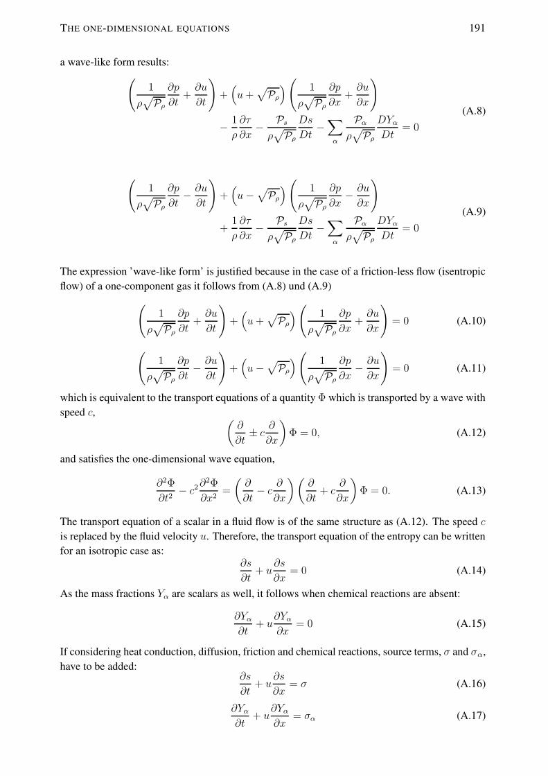
THE ONE-DIMENSIONAL EQUATIONS 191
a wave-like form results:(
1
ρ√Pρ
∂p
∂t+∂u
∂t
)+(u+
√Pρ)( 1
ρ√Pρ
∂p
∂x+∂u
∂x
)
− 1
ρ
∂τ
∂x− Psρ√Pρ
Ds
Dt−∑
α
Pαρ√Pρ
DYαDt
= 0
(A.8)
(1
ρ√Pρ
∂p
∂t− ∂u
∂t
)+(u−
√Pρ)( 1
ρ√Pρ
∂p
∂x− ∂u
∂x
)
+1
ρ
∂τ
∂x− Psρ√Pρ
Ds
Dt−∑
α
Pαρ√Pρ
DYαDt
= 0
(A.9)
The expression ’wave-like form’ is justified because in the case of a friction-less flow (isentropicflow) of a one-component gas it follows from (A.8) und (A.9)
(1
ρ√Pρ
∂p
∂t+∂u
∂t
)+(u+
√Pρ)( 1
ρ√Pρ
∂p
∂x+∂u
∂x
)= 0 (A.10)
(1
ρ√Pρ
∂p
∂t− ∂u
∂t
)+(u−
√Pρ)( 1
ρ√Pρ
∂p
∂x− ∂u
∂x
)= 0 (A.11)
which is equivalent to the transport equations of a quantity Φ which is transported by a wave withspeed c, (
∂
∂t± c ∂
∂x
)Φ = 0, (A.12)
and satisfies the one-dimensional wave equation,
∂2Φ
∂t2− c2∂
2Φ
∂x2=
(∂
∂t− c ∂
∂x
)(∂
∂t+ c
∂
∂x
)Φ = 0. (A.13)
The transport equation of a scalar in a fluid flow is of the same structure as (A.12). The speed cis replaced by the fluid velocity u. Therefore, the transport equation of the entropy can be writtenfor an isotropic case as:
∂s
∂t+ u
∂s
∂x= 0 (A.14)
As the mass fractions Yα are scalars as well, it follows when chemical reactions are absent:
∂Yα∂t
+ u∂Yα∂x
= 0 (A.15)
If considering heat conduction, diffusion, friction and chemical reactions, source terms, σ and σα,have to be added:
∂s
∂t+ u
∂s
∂x= σ (A.16)
∂Yα∂t
+ u∂Yα∂x
= σα (A.17)

192 APPENDIX: THE CHARACTERISTIC FORM OF THE NAVIER-STOKES EQUATIONS
These source terms are further determined in Sect. A.3. Adding and subtracting the Eqs. (A.8)and (A.9) to and from each other, results in the system of the one-dimensional Navier-Stokesequations in a wave-like form,
∂p
∂t= −ρ
√Pρ
2
(X+ +X−
)+ Psσ +
∑
α
Pασα
∂u
∂t= −1
2
(X+ −X−
)+
1
ρ
∂τ
∂x∂s
∂t= −Xs + σ
∂Yα∂t
= −Xα + σα,
(A.18)
with the wave amplitudes
X± =(u±
√Pρ)( 1
ρ√Pρ
∂p
∂x± ∂u
∂x
)
Xs = u∂s
∂x
Xα = u∂Yα∂x
(A.19)
The system can be completed by a transport equation for the temperature in order to circumventthe determination of the temperature from a non-linear polynomial expression relating the entropywith the temperature [66]. It is derived from a state relation T = T (p, s, Yα):
∂T
∂t= Ts
∂s
∂t+ Tp
∂p
∂t+∑
α
Tα∂Yα∂t
(A.20)
The coefficients are again partial derivatives,
Ts =
(∂T
∂s
)
p,Yα
Tp =
(∂T
∂p
)
s,Yα
Tα =
(∂T
∂Yα
)
p,s,Yβ 6=α
, (A.21)
which are determined in Sect. A.4. It is obvious that when the temporal derivatives of pressure,entropy and mass fractions are known from Eqs. (A.18), the temporal derivative of the temper-ature can be computed from Eq. (A.20). Finally, the density can then be computed from theequation of state, in the present case Eq. (2.5) for an ideal gas.
A.2 The three-dimensional equations in Cartesian coordinates
The way to derive the three-dimensional transport equations corresponds to the one followed inSect. A.1 for the one-dimensional equations. Therefore, only the result is given here with thecoordinates denoted as x1, x2 and x3 and the velocity components u1, u2 and u3:
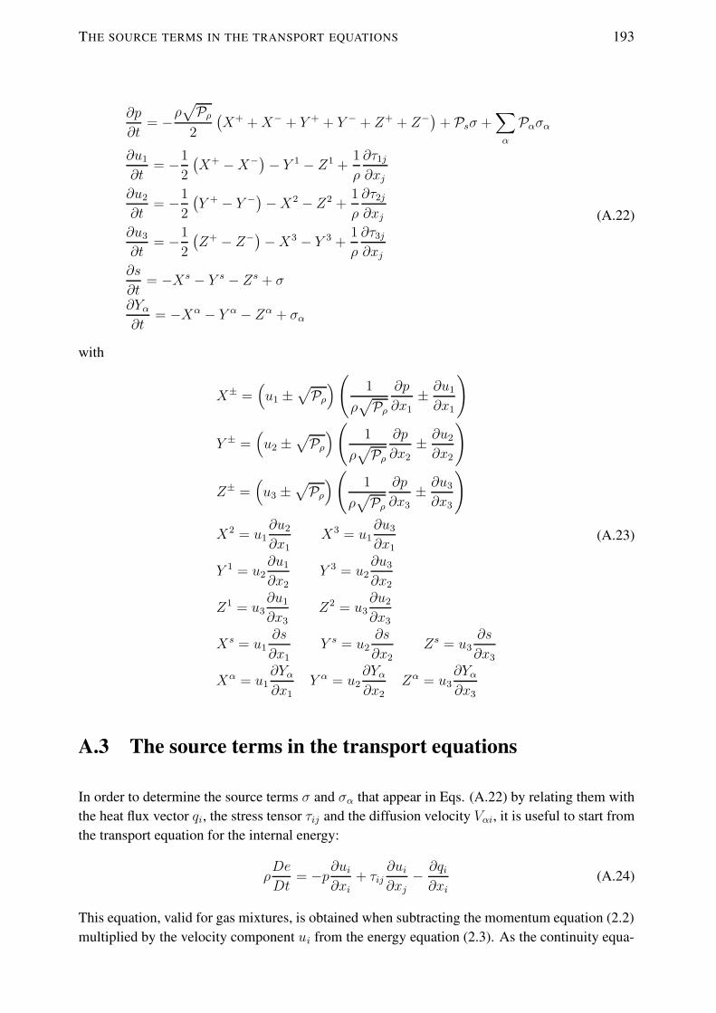
THE SOURCE TERMS IN THE TRANSPORT EQUATIONS 193
∂p
∂t= −ρ
√Pρ
2
(X+ +X− + Y + + Y − + Z+ + Z−
)+ Psσ +
∑
α
Pασα
∂u1
∂t= −1
2
(X+ −X−
)− Y 1 − Z1 +
1
ρ
∂τ1j
∂xj∂u2
∂t= −1
2
(Y + − Y −
)−X2 − Z2 +
1
ρ
∂τ2j
∂xj∂u3
∂t= −1
2
(Z+ − Z−
)−X3 − Y 3 +
1
ρ
∂τ3j
∂xj∂s
∂t= −Xs − Y s − Zs + σ
∂Yα∂t
= −Xα − Y α − Zα + σα
(A.22)
with
X± =(u1 ±
√Pρ)( 1
ρ√Pρ
∂p
∂x1± ∂u1
∂x1
)
Y ± =(u2 ±
√Pρ)( 1
ρ√Pρ
∂p
∂x2± ∂u2
∂x2
)
Z± =(u3 ±
√Pρ)( 1
ρ√Pρ
∂p
∂x3± ∂u3
∂x3
)
X2 = u1∂u2
∂x1X3 = u1
∂u3
∂x1
Y 1 = u2∂u1
∂x2
Y 3 = u2∂u3
∂x2
Z1 = u3∂u1
∂x3
Z2 = u3∂u2
∂x3
Xs = u1∂s
∂x1
Y s = u2∂s
∂x2
Zs = u3∂s
∂x3
Xα = u1∂Yα∂x1
Y α = u2∂Yα∂x2
Zα = u3∂Yα∂x3
(A.23)
A.3 The source terms in the transport equations
In order to determine the source terms σ and σα that appear in Eqs. (A.22) by relating them withthe heat flux vector qi, the stress tensor τij and the diffusion velocity Vαi, it is useful to start fromthe transport equation for the internal energy:
ρDe
Dt= −p∂ui
∂xi+ τij
∂ui∂xj− ∂qi∂xi
(A.24)
This equation, valid for gas mixtures, is obtained when subtracting the momentum equation (2.2)multiplied by the velocity component ui from the energy equation (2.3). As the continuity equa-

194 APPENDIX: THE CHARACTERISTIC FORM OF THE NAVIER-STOKES EQUATIONS
tion (2.1) can be transformed to
p∂ui∂xi
= −pρ
(∂ρ
∂t+ ui
∂ρ
∂xi
)
= −pρ
Dρ
Dt,
(A.25)
Eq. (A.24) can be reformulated as
ρ
(De
Dt− p
ρ2
Dρ
Dt
)= τij
∂ui∂xj− ∂qi∂xi
(A.26)
The left-hand-side (LHS) of this equation can rewritten with the help of the Gibbs fundamentalequation. This equation is for a gas mixture:
de+ pd
(1
ρ
)= Tds+
∑
α
µαWα
dYα (A.27)
with the chemical potentials µα of the species (see Sect. A.4). Thus, in a system with fluidmotions, the substantial derivatives are related by
De
Dt− p
ρ2
Dρ
Dt= T
Ds
Dt+∑
α
µαWα
DYαDt
. (A.28)
This is inserted into the LHS of Eq. (A.24). At the same time it is taken into account that itfollows from Eqs. (A.16) und (A.17) that
Ds
Dt=∂s
∂t+ ui
∂s
∂xi= σ
DYαDt
=∂Yα∂t
+ ui∂Yα∂xi
= σα.
(A.29)
Thus,
ρ
(Tσ +
∑
α
µαWα
σα
)= τij
∂ui∂xj− ∂qi∂xi
(A.30)
from which an equation for the source term σ can be obtained:
σ =1
T
(1
ρ
(τij∂ui∂xj− ∂qi∂xi
)−∑
α
µαWα
σα
)(A.31)
The stress tensor τij is given by Eq. (2.6) and the heat flux vector qi by (2.10).
In order to determine the source terms σα, one starts with the transport equation of the speciesmass fractions (2.4), the LHS of which is simplified with the help of the continuity equation (2.1):
∂ρYα∂t
+∂ρYαui∂xi
= Yα∂ρ
∂t+ ρ
∂Yα∂t
+ Yα∂ρui∂xi
+ ρui∂Yα∂xi
= ρ∂Yα∂t
+ ρui∂Yα∂xi
+ Yα
(∂ρ
∂t+∂ρui∂xi
)
= ρ∂Yα∂t
+ ρui∂Yα∂xi
= ρσα
(A.32)

SPECIFICATION OF THE TRANSPORT EQUATIONS FOR AN IDEAL GAS MIXTURE 195
In the last step, Eq. (A.17) was used. Together with the RHS of the transport equation of thespecies mass fractions (2.4), the final result for the source terms σα is:
σα = −1
ρ
∂
∂xi(ρYαVαi) (A.33)
When taking into account chemical reactions, then
σα =1
ρ
(− ∂
∂xi(ρYαVαi) + ωα
)(A.34)
with the mass production rate of species α, ωα.
A.4 Specification of the transport equations for an ideal gasmixture
In this section, the partial derivatives (A.2) and (A.21), which are necessary for the integration ofthe transport equation, are evaluated for an ideal gas mixture.
Pressure and density are determined unambiguously by the density, the entropy and the speciesmass fractions: p = p (ρ, s, Yα) and ρ (p, s, Yα). The partial derivative of the pressure with respectto the density can be expressed with the help of the speed of sound c as:
Pρ =∂p
∂ρ= c2 = γ (T )RT (A.35)
γ (T ) = cp (T ) /cv (T ) is the ratio of the specific heat capacities cp (T ) und cv (T ) of the mixtureat constant pressure and volume, respectively. The derivative of the pressure with respect to theentropy is transformed to:
Ps =∂p
∂s=∂p
∂T· ∂T∂e· ∂e∂s
= ρR · 1
cv· ∂e∂s
(A.36)
In the last step, the ideal gas law (2.5) and the dependence of the internal energy on the tempera-ture for constant mass fractions, de = cvdT was used. To determine its derivative with respect tothe entropy, the Gibbs fundamental equation (A.27) is taken into account, which is simplified forconstant density ρ and constant mass fractions to de = Tds. Thus, ∂e
∂s= T and
Ps = ρR · 1
cv· T =
p
cv. (A.37)
To determine the partial derivative of the pressure with respect to each mass fraction, the Gibbsfundamental equation is used again, this time written with the specific enthalpy h:
dh = Tds+1
ρdp+
∑
α
µαWα
dYα (A.38)
Keeping the entropy and all but one mass fraction constant, dh = 1ρdp + µα
WαdYα or dp =
ρ(dh− µα
WαdYα
)is obtained. It follows that
Pα =∂p
∂Yα= ρ
(∂h
∂Yα− µαWα
)= ρ
(hα + cp
∂T
∂Yα− µαWα
)(A.39)

196 APPENDIX: THE CHARACTERISTIC FORM OF THE NAVIER-STOKES EQUATIONS
as the specific enthalpy is a function of both, the mass fractions and the temperature: dh =
cpdT +∑
α hαdYα. To compute the partial derivative of the temperature with respect to eachmass fraction, the dependence of the specific internal energy on the temperature and the massfractions is useful: de = cvdT +
∑α eαdYα. Thus,
∂T
∂Yα=
1
cv
(∂e
∂Yα− eα
). (A.40)
Together with the Gibbs fundamental equation (A.27), which is reduced to de = µαWαdYα when
keeping the density and all mass fractions but one constant,
∂T
∂Yα=
1
cv
(µαWα− eα
)(A.41)
is obtained. The internal energy of each species, eα, can be computed from the species enthalpyby eα = hα − R
WαT . Substituting Eq. (A.41) into Eq. (A.39), the result for the partial derivative
of the pressure with respect to each species is:
Pα = ρ
(hα +
cpcv
(µαWα
− eα)− µαWα
)(A.42)
The partial derivative of the temperature with respect to the entropy is given by:
Ts =∂T
∂s=∂T
∂h· ∂h∂s
=T
cp(A.43)
Here, the relation dh = cpdT for constant mass fractions is used, as well as the Gibbs fundamentalequation (A.38) which is reduced to dh = Tds for constant pressure and constant mass fractions.To determine the partial derivative of the temperature with respect to the pressure, dh = cpdT aswell as the Gibbs fundamental equation (A.38), this time for constant entropy and constant massfractions, namely dh = 1
ρdp, are needed:
Tp =∂T
∂p=∂T
∂h· ∂h∂p
=1
ρcp(A.44)
The last partial derivative is the one of the temperature with respect to each species mass fraction.Equation A.41 is not the relation that is asked for here, as it was obtained by keeping the densityconstant. Instead, the pressure has to be kept constant. Together with the assumption of constantentropy and all species but one mass fraction constant, the Gibbs fundamental equation (A.38) isreduced to dh = µα
WαdYα or ∂h
∂Yα= µα
Wα. This is substituted into
∂T
∂Yα=
1
cp
(∂h
∂Yα− hα
)(A.45)
resulting from the dependence of the specific enthalpy on temperature and species mass fractions,dh = cpdT +
∑α hαdYα. The final result is
∂T
∂Yα=
1
cp
(µαWα
− hα). (A.46)

NON-REFLECTING BOUNDARY CONDITIONS 197
In the following, the chemical potentials µα, appearing in Eqs. A.31, A.42 and A.46 are deter-mined for ideal gases. From the Gibbs fundamental equation, written for the free enthalpy G of agas mixture in a control volume V with the mole numbers nα of the individual components,
dG = −SdT + V dp+∑
α
µαdnα, (A.47)
the relation
µα =
(∂G
∂nα
)
p,T,nβ 6=α
(A.48)
is obtained. The free enthalpy of the mixture is given by
G = H − TS =∑
α
nα (Hα − TSα) (A.49)
where H and S are the molar enthalpy and the molar entropy, respectively. H and S are theentropy and the enthalpy, and n is the total mole number of the mixture in the control volume. InEq. (A.49), the entropy due to the mixing of the gas components is neglected. Only the entropiesof the individual gas components, Sα are taken into account. Computing the derivative of Eq.(A.49), leads to
µα =
(∂G
∂nα
)
p,T,nβ 6=α
= Hα − TSα. (A.50)
Thus, written in specific quantities, the chemical potentials are
µα = Wα (hα − Tsα) (A.51)
wherein the enthalpies hα and the entropies sα are computed as polynomials of the temperature[66].
A.5 Non-reflecting boundary conditions
Besides the periodic boundaries used in the streamwise and spanwise directions, only non-reflectingboundaries in the transverse direction are required for DNS and LES of temporally evolving shearlayers. Their treatment is facilitated by the particular wave-like formulation of the Navier-Stokesequations (A.22). Wave amplitudes at the boundaries, the direction of which is into the computa-tional domain, are set to zero. At the lower x3-boundary, it is
Z+ = 0, if u3 + c ≥ 0
Z− = 0, if u3 − c ≥ 0
Z1 = Z2 = Zs = Zα = 0, if u3 ≥ 0
(A.52)
and at the upper x3-boundary
Z+ = 0, if u3 + c ≤ 0
Z− = 0, if u3 − c ≤ 0
Z1 = Z2 = Zs = Zα = 0, if u3 ≤ 0.
(A.53)

Bibliography
[1] Adams, N.A., Leonard, A., 1999, Deconvolution of subgrid-scales for the simulation ofshock-turbulence interaction. In: Direct and Large-Eddy Simulation III, Eds: Voke, P., Sand-ham, N.D. and Kleiser, L.. Kluwer, Dordrecht, 201-212.
[2] Adams, N.A., Stolz, 2002, A sub-grid deconvolution approach for shock capturing, J. Com-put. Phys. 178, 391-426.
[3] Angelbergerer, C., Veynante, D., Egolfopoulos, F., 2000, LES of chemical and acoustic forc-ing of a premixed dump combustor, Flow Turbul. Combust. 65, 205-222.
[4] Barlow, R.S., Fourguette, D.C., Mungal, M.G., Dibble, R.W., 1992, Experiments on thestructure of an annular compressible reacting shear layer, AIAA J. 30, 2244-2251.
[5] Barlow, R.S., Fiechtner, G.J., Carter, C.D., Chen, J.-Y., 2000, Experiments on the ScalarStructure of Turbulent CO/H2/N2 Jet Flames, Combust. Flame 120, 549-569.
[6] Barre, S., Quine, C., Dussauge, J.P., 1994, Compressibility effects on the structure of super-sonic mixing layers: experimental results, J. Fluid Mech. 259, 47-78.
[7] Bell, J.H., Mehta, R.D., 1990, Development of a two-stream mixing layer from tripped anduntripped boundary layers, AIAA J., 28, 2034-2042.
[8] Bilger, R.W., 1976, The structure of diffusion flames, Combust. Sci. Technol. 13, 155-170.
[9] Bilger, R.W., 1980, Turbulent flows with nonpremixed reactants. In: Topics in AppliedPhysics Number 44, Eds: Libby, P.A, Williams, F.A., Springer, New York, 65-113.
[10] Bilger, R.W., 1993, Conditional moment closure for turbulent reacting flow, Phys. Fluids A5, 436-444.
[11] Bilger, R.W., Starner, S.H., Kee, R.J., 1990, On reduced mechanisms for methane-air com-bustion in nonpremixed flames, Combust. Flame 80, 135-149.
[12] Blaisdell, G.A., Mansour, N.N., Reynolds, W.C., 1991, Numerical simulation of compress-ible homogeneous turbulence, Report No. TF-50, Stanford University, Stanford, CA.
[13] Blaisdell, G.A., Mansour, N.N., Reynolds, W.C., 1993, Compressibility effects on thegrowth and structure of homogeneous turbulent shear flow, J. Fluid Mech. 256, 443-485.
[14] Bogdanoff, D.W., 1983, Compressibility effects in turbulent shear layers, AIAA J. 21, 926-927.
[15] Bonnet, J.P., Debisschop, J.R., Chambres, O., 1993, Experimental studies of the turbulentstructure of supersonic mixing layers, AIAA Paper 93-0217.

BIBLIOGRAPHY 199
[16] Bradshaw, P., 1977, Compressible turbulent shear layers, Ann. Rev. Fluid Mech., 9, 33-54.
[17] Branley, N., Jones, W., 2001, Large eddy simulation of a turbulent non-premixed flame,Combust. Flame 127, 1914-1934.
[18] Breidenthal, R., 1981, Structure in turbulent mixing layers and wakes using a chemicalreaction, J. Fluid Mech. 109, 1-24.
[19] Browand, F.K., Troutt, T.R., 1985, The turbulent mixing layer: Geometry of the large vor-tices, J. Fluid Mech. 158, 489-509.
[20] Brown, G., 1974, The entrainment and large structure in turbulent mixing layers. In: 5thAustralasian Conf. on Hydraulics and Fluid Mechanics, Eds: Lindley, D., Sutherland, A.J.,352-359.
[21] Brown, G.L., Roshko, A., 1974, On density effects and large structure in turbulent mixinglayers, J. Fluid Mech. 64, 775-816.
[22] Burke, S.P., Schumann, T.E.W., 1928, Diffusion flames, Industrial and Engineering Chem-istry 20, 998-1005.
[23] Bushe, W.K., Steiner, H., 1999, Conditional moment closure for large eddy simulation ofnonpremixed turbulent reacting flows, Phys. Fluids 11, 1896- 1906.
[24] Calhoon, W., Menon, S., 1996, Subgrid Modeling for Reacting Large Eddy Simulations,AIAA Paper 96-0516.
[25] Chambres, O., Barre, S., Bonnet, J., 1998, Detailed turbulence characteristics of a highlycompressible supersonic turbulent plane mixing layer, J. Fluid Mech., submitted.
[26] Chen, J.Y., Kollman, W., Dibble, R.W., 1989, Pdf modeling of turbulent methane-air non-premixed jet flames, Combust. Sci. Technol. 64, 315-346.
[27] Clemens, N.T., Mungal, M.G., 1995, Large-scale structure and entrainment in the super-sonic mixing layer, J. Fluid Mech. 284, 171-216.
[28] Clemens, N.T., Paul, P.H., 1995, Scalar measurements in compressible axysymmetric mix-ing layers, Phys. Fluids A 7, 1071-1081.
[29] Colucci, P.J., Jaberi, F.A., Givi, P., Pope, S.B., Filtered density function for large eddysimulation of turbulent reacting flows, Phys. Fluids 10, 499-515.
[30] Cook, A.W., 1997, Determination of the constant coefficient in scale similarity models ofturbulence, Phys. Fluids 9, 1485-1487.
[31] Cook, A.W., Riley, J.J., 1994, A subgrid model for equilibrium chemistry in turbulent flows,Phys. Fluids 6, 2868-2870.
[32] Cook, A.W., Riley, J.J., 1998, Subgrid-scale modeling for turbulent reacting flows, Combust.Flame 112, 593-606.
200 BIBLIOGRAPHY
[33] Cook, A.W., Riley, J.J., Kosaly, G., 1997, A laminar flamelet approach to subgrid-scalechemistry in turbulent flows, Combust. Flame 109, 332-341.
[34] Cuenot, B., Poinsot, T., 1996, Asymptotic and Numerical Study of Diffusion Flames withVariable Lewis Number and Finite Rate Chemistry, Combust. Flame 104, 111-137.
[35] Day, M.J., Mansour, N.N., Reynolds, W.C., 2001, Nonlinear stability and structure of com-pressible reacting mixing layers, J. Fluid Mech. 446, 375-408.
[36] Debisschop, J.R., Bonnet, J.P., 1993, Mean and fluctuating velocity measurements in super-sonic mixing layers. In: Engineering Turbulence Modelling and Experiments 2, Eds: Rodi,W., Martelli, F., Elsevier.
[37] de Bruyn Kops, S.M., Riley, J.J., Kosaly, G., 1998, Investigation of modeling for non-premixed turbulent combustion, Flow Turbul. Combust. 60, 105-122.
[38] de Bruyn Kops, S.M., Riley, J.J., Kosaly, G., 2001, Direct numerical simulation of reactingscalar mixing layers, Phys. Fluids 13, 1450-1465.
[39] de Bruyn Kops, S.M., Riley, J.J., 2003, Large-Eddy Simulation of a Reacting Scalar MixingLayer with Arrhenius Chemistry, Computers and Mathematics with Applications 46, 547-569.
[40] de Charentenay, J., Ern, A., 2002, Multicomponent transport impact on turbulent premixedH2/O2 flames, Combust. Theor. Model. 6 439-462.
[41] DesJardin P.E., Frankel, S.H., 1998, Large eddy simulation of a nonpremixed reacting jet:Application and assessment of subgrid-scale combustion models, Phys. Fluids 10, 2298-2314.
[42] Di Mare, F., Jones, W., Menzies, K., 2004, Large eddy simulation of a model gas turbinecombustor, Combust. Flame, 137, 278-294.
[43] Dimotakis, P., 1984, Two-dimensional shear layer entrainment, AIAA J. 24, 1791-1796.
[44] Dimotakis, P.E., Brown, G.L., 1976, The mixing layer at high Reynold numbers: largestructure dynamics and entrainment, J. Fluid Mech. 78, 535-560.
[45] Dimotakis, P.E., Leonard, A., 1994, Chemical reactions in turbulent mixing flows, GALCITRep. 94-3,. California Institute of Technology, Pasadena, CA.
[46] Domaradzki, J.A., Adams, N.A., 2002, Direct modelling of subgrid scales of turbulence inlarge-eddy simulation, J. Turbulence 3, 024.
[47] Dowling, A.P., 1992, Thermoacoustic Sources and Instabilities. In: Modern Methods inAnalytical Acoustics, Eds: Crighton, D.G., Dowling, A.P., Ffowcs Williams, J.E., Heckl, M.,Leppington, F.G., Springer, 378-405.
[48] El Baz, A.M., Launder, B.E., 1993, Second-moment modelling of compressible mixinglayers. In: Engineering, Turbulence Modelling and Experiments 2, Eds: Rodi, W., Martelli,F., Elsevier.

BIBLIOGRAPHY 201
[49] Elliott, G.S., Samimy, M., 1990, Compressibility effects in free shear layers, Phys. Fluids A2, 1231-1240.
[50] Elliott, G.S., Samimy, M., Arnette, S.A., 1993, Study of compressible mixing layers withfiltered Rayleigh scattering based visualizations, AIAA J. 30, 2567-2569.
[51] Emanuel, G., 1986, Gasdynamics: Theory and Applications, AIAA Education Series, NewYork.
[52] Erdos, G.S., Samimy, M., Arnette, S.A., 1992, Experiments on shear layer mixing at hyper-velocity conditions, AIAA Paper, 92-0628.
[53] Ern, A., Giovangigli, V., 1994, Multicomponent transport algorithms. Springer.
[54] Ern, A., Giovangigli, V., 1995, Fast and accurate multicomponent transport property evalu-ation, J. Comput. Physics 120, 105-116.
[55] Ern, A., Giovangigli, V., 1998, Thermal diffusion effects in hydrogen-air and methane-airflames, Combust. Theory Model. 2, 349-372.
[56] Ern, A., Giovangigli, V., 1999, Impact of detailed multicomponent transport on planar andcounterflow hydrogen/air and methane/air flames, Combust. Sci. Tech. 149, 157-181.
[57] Faeth, G.M., Samuelsen, G.S., 1986, Fast reaction nonpremixed combustion, Prog. EnergyCombust. Sci. 12, 305-372.
[58] Fiedler, H., 1974, Transport of heat across a plane turbulent mixing layer, Adv. Geophys.18A, 93-109.
[59] Forkel, H., Janicka, J., 2000, Large-Eddy Simulation of a Turbulent Hydrogen DiffusionFlame, Flow Turbul. Combust. 65, 163-175.
[60] Foysi, H., Sarkar, S., Friedrich, R., 2004, Compressibility effects and turbulence scaling insupersonic channel flow, J. Fluid Mech. 509, 207-216.
[61] Foysi, H., 2005, Transport passiver Skalare in wandgebundener und isotroper kompressiblerTurbulenz, Dissertation, TU Munchen, Fakultat fur Maschinenwesen, Germany.
[62] Frankel, S.H., Adumitroaie, V., Madinia, C.K., Givi, P., Large-eddy simulation of turbu-lent reacting flows by assumed PDF methods, In: Engineering Applications of Large EddySimulations, Eds: Ragab, S.A., Piomelli, U., ASME, New York.
[63] Freund, J.B., Lele, S.K., Moin, P., 2000, Compressibility effects in a turbulent annular mix-ing layer. Part 1. Turbulence and growth rate, J. Fluid Mech. 421, 229-267.
[64] Freund, J.B., Moin, P., Lele, S.K., 2000, Compressibility effects in a turbulent annular mix-ing layer. Part 2. Mixing of a passive scalar, J. Fluid Mech. 421, 269-292.
[65] Gao, F., O’Brien, E.E., 1993, A large-eddy simulation scheme for turbulent reacting flows,Phys. Fluids A 5, 1282-1284.
[66] Gardiner, W., 1984, Combustion chemistry. Springer, New York.
202 BIBLIOGRAPHY
[67] Givi, P., Madnia, C.K., Steinberger, C.J., Carpenter, M.H., Drummond, J.P., 1991, Effects ofcompressibility and heat release in a high speed reacting mixing layer, Combust. Sci. Technol.78, 33-68.
[68] Goebel, S.G., Dutton, J.C., 1991, Velocity measurements of compressible, turbulent mixinglayers, AIAA J. 29, 538-546.
[69] Girimaji, S.S., Zhou, Y., 1996, Analysis and modeling of subgrid scalar mixing using nu-merical data, Phys. Fluids 8, 1224-1236.
[70] Hall, J.L., Dimotakis, P.E., Rosemann, H., 1991, Some measurements of molecular mixingin compressible turbulent shear layers, AIAA Paper 91-1719.
[71] Hall, J.L., Dimotakis, P.E., Rosemann, H., 1993, Experiments in nonreacting compressibleshear layers, AIAA J. 31, 2247-2254.
[72] Hermanson, J.C., Dimotakis, P.E., 1989, Effects of heat release in a turbulent, reacting shearlayer, J. Fluid Mech. 199, 333-375.
[73] Hilbert, R., Tap, F., El-Rabii H., Thevenin, D., 2004, Impact of detailed chemistry andtransport models on turbulent combustion simulations, Prog. Energy Combust. Sci. 30, 61-117.
[74] Hirschfelder, J.O., Curtiss, C.F., Bird, R.B., 1954, Molecular theoury of gases and liquids.Wiley, New York.
[75] Hussain, A.K.M.F., Zaman, K.M.B.Q., 1985, An experimental study of organized motionsin the turbulent plane mixing layer, J. Fluid Mech. 159, 85-104.
[76] Ihme, M., Cha, C.M., Pitsch, H., 2005, Prediction of local extinction and re-ignition effectsin non-premixed turbulent combustion using a flamelet/progress variable approach, Proc.Combust. Inst. 30, 793-800.
[77] Ihme, M., Pitsch, H., 2005, LES of a non-premixed flame using an extendedflamelet/progress variable model, AIAA Paper 2005-0558.
[78] Island, T.C., 1997, Quantitative scalar measurements and mixing enhancement in compress-ible shear layers, Dissertation, Stanford University, Stanford, USA.
[79] Jaberi, F.A., Miller, R.S., Mashayek, F., Givi, P., 1997, Differential diffusion in binary scalarmixing and reaction. Combustion and Flame 109, 561-577.
[80] Jaberi, F.A., Colucci, P.J., James, S., Givi, P., Pope, S.B., 1999, Filtered mass density func-tion for large-eddy simulation of turbulent reacting flows, J. Fluid Mech. 401, 85-121.
[81] Jackson, T.L., Grosch, C.E., 1989, Inviscid spatial stability of a compressible mixing layer,J. Fluid Mech. 208, 609-637.
[82] Janicka, J., Sadiki, A., 2005, Large eddy simulation of turbulent combustion systems, Proc.Combust. Inst. 30, 537-547.
BIBLIOGRAPHY 203
[83] Jimenez, J., 1983, A spanwise structure in the plane shear layer, J. Fluid Mech. 132, 319-336.
[84] Jimenez, J., Ducros, F., Cuenot, B., Bedat, B., 2001, Subgrid scale variance and dissipationof a scalar field in large eddy simulations, Phys. Fluids 13, 1748-1754.
[85] Jimenez, J., Linan, A., Rogers, M.M., Higuera, F.J., 1997, A priori testing of subgrid modelsfor chemically reacting non-premixed turbulent shear flows, J. Fluid Mech. 349, 149-171.
[86] Kempf, A., Sadiki, A., Janicka, J., 2003, Prediction of finite chemistry effects using largeeddy simulation, Proc. Combust. Inst. 29, 1979-1985.
[87] Kempf, A., Lindtstedt, R.P., Janicka, J., 2006, Large-eddy simulation of a bluff-body stabi-lized nonpremixed flame, Combust. Flame 144, 170-189.
[88] Kerstein, A.R., 1988, A linear-eddy model of turbulent scalar transport and mixing, Com-bust. Sci. Technol. 60, 391-421.
[89] Kim, J., 1989, On the structure of pressure fluctuations in simulated turbulent channel flow,J. Fluid Mech. 205, 421-451.
[90] Kim, W., Menon, S., Mongia, H., 1999, Large-eddy simulation of a gas turbine combustorflow, Combust. Sci. Technol. 143, 25-62.
[91] Kim, S.H., Pitsch, H., 2005, Conditional filtering method for large eddy simulation of tur-bulent nonpremixed combustion, Phys. Fluids, in press.
[92] Klimenko, A.Y., 1990, Multicomponent diffusion of various admixtures in turbulent flow,Fluid Dyn. 25, 3-10.
[93] Klimenko, A.Y., 2001, On the relation between the conditional moment closure and un-steady flamelets, Fluid Dyn. 25 327-334.
[94] Klimenko, A.Y., Bilger, R.W., 1999, Conditional moment closure for turbulent combustion,Prog. Energy Combust. Sci. 25, 595-687.
[95] Kovasznay, L.S.G., 1953, Turbulence in Supersonic Flows, J. Aeronaut. Sci. 20, 657-682.
[96] Lasheras, J.C., Cho, J.S., Maxworthy, T., 1986, On the origin and evolution of streamwisevortical structures in a plane, free shear layer, J. Fluid Mech. 172, 231-258.
[97] Lee, S., Lele, S.K., Moin, P., 1991, Eddy shocklets in decaying compressible turbulence,Phys. Fluids A 3, 657-664.
[98] Lele, S.K., 1989, Direct numerical simulation of compressible free shear flows, AIAA Paper,89-0374.
[99] Lele, S.K., 1992, Compact finite difference schemes with spectral-like resolution, J. Com-put. Phys. 103, 16-42.
[100] Libby, P.A., Williams, F.A., 1994, Turbulent reacting flows. Academic Press, New York.
204 BIBLIOGRAPHY
[101] Lentini, D., 1994, Assessment of the stretched laminar flamelet approach for non-premixedturbulent combustion, Combust. Sci. Technol. 100, 95-122.
[102] Lu, G., Lele, S.K., 1994, On the density effects on the growth rate of compressible mixinglayer, Phys. Fluids 6, 1073-1075.
[103] Mahesh, K., Constantinescu G., Apte, S., Iaccarino, G., Ham, F., Moin, P., 2005, Large-eddy simulation of reacting turbulent flows in complex geometries, ASME J. Appl. Mech., inpress.
[104] Masutani, S.M., Bowman, C.T., 1986, The structure of a chemically reacting plane mixinglayer, J. Fluid Mech. 172, 93-126.
[105] Mathew, J., Basu, A.J., 2002, Some characteristics of entrainment at a cylindrical turbu-lence boundary, Phys. Fluids 14, 2065-2072.
[106] Mathew, J., Lechner, R., Foysi, H., Sesterhenn, J., Friedrich, R., 2003, An explicit filteringmethod for large eddy simulation of compressible flows., Phys. Fluids 15, 2279-2289.
[107] Mathew, J., R., Foysi, H., Friedrich, R., 2006, A new approach to LES based on explicitfiltering, Int. J. Heat Fluid Flow 27, 594-602. w
[108] McMurtry, P.A., Riley, J.J., 1987, Mechanisms by which heat release affects the flow fieldin a chemically reacting, turbulent mixing layer, AIAA Paper, 87-0131.
[109] McMurtry, P., Riley, J., Metcalfe, R., 1989, Effects of heat release on the large-scale struc-ture in turbulent mixing layers, J. Fluid Mech. 199, 297-332.
[110] McMurtry, P.A., Menon, S., Kerstein, A.R., 1992, A linear eddy sub-grid model for turbu-lent reacting flows: Application to hydrogen-air combustion, Proc. Combust. Inst. 24, 271-278.
[111] Mellado, J.P., Sarkar, S., Pantano, C., 2003, Reconstruction subgrid models for non-premixed combustion, Phys. Fluids 15, 3280-3307.
[112] Messerschmith, N.L., Dutton, J.C., Krier, H., 1991, Experimental investigation of largescale structures in compressible mixing layers, AIAA Paper 91-0244.
[113] Miller, J.A., Mitchell, R.E., Smooke, M.D., Kee, R.J., 1982 Toward a comprehensivechemical kinetic mechanism for the oxidation of acetylene: comparison of model predictionswith results from flame and shock tupe experiments Proc. Combust. Inst. 19, 181-196.
[114] Miller, M.F., Bowman, C.T., Mungal, M.G., 1998, An experimental investigation of theeffects of compressibility on a turbulent reacting mixing layer, J. Fluid. Mech. 356, 25-64.
[115] Miller, R.S., Madnia, C.K., Givi, P., 1994, Structure of a Turbulent Reacting Mixing Layer,Combust. Sci. and Tech., 99, 1-36.
[116] Moin, P., Apte, S., 2005, Large-eddy simulation of realistic gas turbine combustors, AIAAJ., in press.
BIBLIOGRAPHY 205
[117] Moin, P., Mahesh, K., 1998, Direct Numerical Simulation: A Tool in Turbulence Research,Annu. Rev. Fluid. Mech. 30, 539-578.
[118] Mungal, M.G., Dimotakis, P.E., 1984, Mixing and combustion with low heat release in aturbulent shear layer, J. Fluid Mech. 148, 349-382.
[119] Nilsen, V., Kosaly, G., 1999, Differential Diffusion in Turbulent Reacting Flows, Combust.Flame 117, 493-513.
[120] Pantano, C., 2000, Compressibility effects in turbulent nonpremixed reacting shear flows,Dissertation, University of California, San Diego, USA.
[121] Pantano, C., 2006, An additive semi-implicit Runge-Kutta family of schemes for nonstiffsystems, , Applied Numerical Mathematics, in press.
[122] Pantano, C., Sarkar, S., 2001, A subgrid model for nonlinear functions of a scalar, Phys.Fluids 13, 3803-3819.
[123] Pantano, P., Sarkar, S., 2002, A study of compressibility effects in the high-speed turbulentshear layer using direct simulation, J. Fluid Mech. 451, 329-371.
[124] Pantano, C., Sarkar, S., Williams, F.A., 2003, Mixing of a conserved scalar in a turbulentreacting shear layer, J. Fluid Mech. 481, 291-328.
[125] Papmoschou, D., 1995, Evidence of shocklets in a counterflow supersonic shear layer,Phys. Fluids 7, 233-235.
[126] Papamoschou, D., Roshko, A., 1988, The compressible turbulent shear layer: an experi-mental study, J. Fluid Mech. 197, 453-477.
[127] Passot, T., Pouquet, A., 1987, Numerical simulation of compressible homogeneous flowsin the turbulent regime, J. Fluid Mech. 181, 441-466.
[128] Peters, N., 1984, Laminar diffusion flamelet models in non-premixed turbulent combus-tion, Prog. Energy Combust. Sci. 10, 319-339.
[129] Peters, N., 2000, Turbulent combustion, Cambridge University Press.
[130] Pierce, C.D., Moin, P., 1998, A dynamic model for subgrid-scale variance and dissipationrate of a conserved scalar, Phys. Fluids 10, 3041-3044.
[131] Pierce C.D., Moin, P., 2001, Progress-variable approach for large eddy simulation of tur-bulent combustion, Report No. TF-80, Stanford University, Stanford, CA.
[132] Pierce, C.D., Moin, P., 2004, Progress-variable approach for large-eddy simulation of non-premixed turbulent combustion, J. Fluid Mech. 504, 73-97.
[133] Pitsch, H., 2000, Unsteady flamelet modeling of differential diffusion in turbulent jet dif-fusion flames, Combust. Flame 123, 358-374.
[134] Pitsch, H., 2002, Improved pollutant predictions in large-eddy simulations of turbulentnon-premixed combustion by considering scalar dissipation rate fluctuations, Proc. Combust.Inst. 29, 1971-1978.

206 BIBLIOGRAPHY
[135] Pitsch, H., 2006, Large-Eddy Simulation of Turbulent Combustion, Annu. Rev. Fluid.Mech. 38, 453-482.
[136] Pitsch, H., Chen, M., Peters, N., 1998, Unsteady flamelet modeling of turbulent hydro-gen/air diffusion flames, Proc. Combust. Inst. 27, 1057-1064.
[137] Pitsch, H., Ihme, M., 2005, An unsteady/flamelet progress variable method for LES ofnonpremixed turbulent combustion, AIAA Paper 2004-557.
[138] Pitsch, H., Peters, N., 1998, A consistent flamelet formulation for non-premixed combus-tion considering differential diffusion effects, Combust. Flame 114, 26-40.
[139] Pitsch, H., Steiner, H., 2000, Large-eddy simulation of a turbulent piloted methane/airdiffusion flame (Sandia flame D), Phys. Fluids 12, 2541-2554.
[140] Pitsch, H., Steiner, H., 2000, Scalar mixing and dissipation rate in large-eddy simulationsof non-premixed turbulent combustion, Proc. Combust. Inst. 28, 41-49.
[141] Planche, O.H., Reynolds, W.C., 1992, A numerical investigation of the compressible re-acting mixing layer, Report No. TF-56, Stanford University, Stanford, CA.
[142] Poinsot, T., Veynante, D., 2001, Theoretical and numerical combustion. R.T. Edwards.
[143] Pope, S.B., 1985, PDF methods for turbulent reactive flows, Prog. Energy Combust. Sci.11, 119-192.
[144] Pope, S.B., 1990, Computations of turbulent combustion: progress and challenges, Proc.Combust. Inst. 23, 591-612.
[145] Pope, S.B., 2000, Turbulent Flows, Cambridge University Press.
[146] Pope, S.B., 2004, Ten questions concerning the large-eddy simulation of turbulent flows,New J. Phys. 6, 1-24.
[147] Ragab, S.A., Wu, J.L., 1989, Linear instabilities in two-dimensional compressible mixinglayers, Phys. Fluids A 1, 957-966.
[148] Red, R.C., Prausnitz, J.M, Poling, B.E., 1988, The properties of gases and liquids. McGrawHill.
[149] Reveillon, J., Vervisch, L., 1996, Response of the dynamic LES model to heat releaseinduced effects, Phys. Fluids A 8, 2248-2250.
[150] Reveillon, J., Vervisch, L., 1996, Subgrid-scale turbulent micromixing: dynamic approach,AIAA J. 36, 336-341.
[151] Riley, J.J., Metcalfe, R.W., Orszag, S.A., 1986, Direct numerical simulations of chemicallyreacting turbulent mixing layers, Phys. Fluids 29, 406-422.
[152] Rogers, M.M., Moser, R.D., 1994, Direct simulation of a self-similar turbulent mixinglayer, Phys. Fluids 6, 903-923.
[153] Rotta, J.C., 1972, Turbulente Stromungen, Teubner-Verlag, Stuttgart.

BIBLIOGRAPHY 207
[154] Sagaut, P., 2006, Large Eddy Simulation for Incompressible Flows, Springer, Berlin Hei-delberg.
[155] Samimy, M., Elliott, G.S., 1990, Effects of compessibility on the characteristics of freeshear layers, AIAA J. 28, 439-445.
[156] Samimy, M., Reeder, M.F., Elliott, G.S., 1992, Compressibility effects on large structuresin free shear flow, Phys. Fluids A 4, 1251-1258.
[157] Sandham, N.D., Reynolds, W.C., 1991, Compressible mixing layer: Linear theory anddirect simulation, AIAA J. 28, 618-624.
[158] Sandham, N.D., Reynolds, W.C., 1991, Three-dimensional simulations of large-eddies inthe compressible mixing layer, J. Fluid Mech. 224, 133-158.
[159] Sandham, N.D., Yee, H.C., 1989, A numerical study of a class of TVD schemes for com-pressible mixing layers, NASA Tech. Rep. 102194.
[160] Sarkar, S., 1992, The pressure-dilatation correlation in compressible flows, Phys. Fluids A2, 2674-2682.
[161] Sarkar, S., 1995, The stabilizing effect of compressibility in turbulent shear flow, J. FluidMech. 282, 163-186.
[162] Sarkar, S., 1997, On density and pressure fluctuations in uniformly sheared compressibleflow. In: IUTAM Symposium on Variable Density Low-Speed Turbulent Flows., Eds: Fu-lachier, L. et al., Kluwer, 325-332.
[163] Sarkar, S., 2002, The high-speed turbulent shear layer. In: Variable Density Fluid Turbu-lence, Fluid Mechanics and its Applications. 69, Eds: Chassaing, P., Antonia, R.A., Ansel-met, F., Joly, L., Sarkar, S., Kluwer, 235-259.
[164] Sarkar, S., Erlebacher, G., Hussaini, M.Y., 1991, Direct simulation of compressible turbu-lence in a shear flow, Theor. Comput. Fluid Dynamics 2, 291-305.
[165] Saxena, V., Pope, S.B., 1998, Pdf calculations of major and minor species in a turbulentpiloted jet flame, Proc. Combust. Inst. 27, 1081-1086.
[166] Schmidt, H., Schumann, U., 1989, Coherent structure of the convective boundarylayerderived from large-eddy simulations, J. Fluid Mech. 200, 511-562.
[167] Sesterhenn, J., 2000, A characteristic-type formulation of the Navier-Stokes equations forhigh order upwind schemes, Computers & Fluids 30, 37-67.
[168] Sheikhi, M.R.H., Drozda, T.G., Givi, P., Pope, S.B., 2003, Velocity-scalar filtered densityfunction for large eddy simulation of turbulent flows, Phys. Fluids 15, 2321-2337.
[169] Shinjo, J., Mizobuchi, Y., Ogawa, S., 2003, LES of unstable combustion in a gas turbinecombustor, High Perform. Comput. 2858, 234-244.

208 BIBLIOGRAPHY
[170] Smith, L.L., Dibble, R.W., Talbot, L., Barlow, R.S., Carter, C.D., 1995, Laser RamanScattering Measurements of Differential Molecular Diffusion in Turbulent Nonpremixed JetFlames of H2/ CO2 Fuel, Combust. Flame 100, 153-160.
[171] Sommerer, Y., Galley, D., Poinsot, T., Ducruix, S., Lacas, F., Veynante, D., 2004, Largeeddy simulation and experimental study of flashback and blow-off in a lean partially premixedswirled burner, J. Turb. 5, 037.
[172] Spencer, B. W., Jones, B. G., 1971, Statistical investigation of pressure and velocity fieldsin the turbulent two-stream mixing layer, AIAA Paper 71-613.
[173] Sreenivasan, K.R., Meneveau, C., 1986, The fractal facets of turbulence, J. Fluid Mech.173, 357-386.
[174] Sripakagorn, P., Mitarai, S., Kosaly, G., Pitsch, H., 2004, Extinction and reignition in adiffusion flame (a direct numerical study), J. Fluid Mech. 518, 231-259.
[175] Stolz, S., Adams, N.A., 1999, An approximate deconvolution procedure for Large-Eddysimulation, Phys. Fluids 11, 1699-1701.
[176] Stolz, S., Adams, N.A., Kleiser, L., 2001, An approximate deconvolution model for large-eddy simulation with application to incompressible wall-bounded flows, Phys. Fluids 13,997-1015.
[177] Stolz, S., Adams, N.A., Kleiser, L., 2001, An approximate deconvolution model for LESof compressible flow and its application to shock-turbulence interaction, Phys. Fluids 13,2985-3001.
[178] Stone, C., Menon, S., 2003, Open-loop control of combustion instabilities in a model gasturbine combustor, J. Turb. 4, 020.
[179] Sutherland, J.C., 2004, Evaluation of mixing and reaction models for large-eddy simulationof nonpremixed combustion using direct numerical simulation. Dissertation, University ofUtah, USA.
[180] Vervisch, L., Veynante, D., 1998, Direct numerical simulation of non-premixed turbulentflames, Annu. Rev. Fluid Mech. 30 655-691.
[181] Veynante, D., Vervisch, L., 2002, Turbulent combustion modeling, Prog. Energy Combust.Sci. 28, 193-266.
[182] Vreman, B., Kuerten, H., Geurts, B., 1995, Shocks in direct numerical simulation of theconfined three-dimensional mixing layer, Phys. Fluids 7, 2105-2107.
[183] Vreman, A.W., Sandham, N.D., Luo, K.H., 1996, Compressible mixing layer growth rateand turbulence characteristics, J. Fluid Mech. 320, 235-258.
[184] Wall, C., Boersma, B.J., Moin, P., 2000, An evolution of the assumed beta probabilitydensity function subgrid-scale model for large eddy simulation of nonpremixed, turbulentcombustion with heat release, Phys. Fluids 12, 2522-2529.

BIBLIOGRAPHY 209
[185] Wall, C.T., Moin, P., 2005, Numerical methods for large eddy simulation of acoustic com-bustion instabilities, Report No. TF-91, Stanford University, Stanford, CA.
[186] Westerweel, J., Fukushima, C., Pedersen, J.M., Hunt, J.C.R., 2005, Mechanics of theTurbulent-Nonturbulent Interface of a Jet, Physical Review Letters PRL 95, 174501.
[187] Williams, F.A., 1985, Combustion theory., Addison Wesley.
[188] Williamson, J., 1980, Low-storage Runge-Kutta schemes, J. Comput. Phys. 35, 48-56.
[189] Wygnanski, I., Oster, D., Fiedler, H., Dziomba, B., 1979, On the perseverance of a quasi-two-dimensional eddy-structure in a turbulent mixing layer, J. Fluid Mech. 93, 325-335.
[190] Xu, J., Pope, S.B., 2000, PDF calculations of turbulent nonpremixed flames with localextinction, Combust. Flame 123, 281-307.
[191] Yeung, P.K., Pope S.B., 1988, An algorithm for tracking fluid particles in numerical simu-lations of homogeneous turbulence, J. Comput. Physics 79,373-416.
[192] Zeman, O., 1990, Dilatational dissipation - the concept and application in modelling com-pressible mixing layers, Phys. Fluids A 2, 178-188.