Czech Technical University inPrague

Faculty of Electrical Engineering

Department of control Engineering

Diploma Thesis

Performance comparison of Extended andUnscented Kalman Filter implementation in

INS-GPS integration

Erasmus Mundus Programme

SpaceMaster

Prague,2009 Author: Joshy Madathiparambil Jose

Declaration

I, Joshy M. Jose, honestly declare that I have worked out my diploma the-sis individually and all resources (literature,projects,SW etc) that I used arestated in the attached list.

InPrague, dateSignature

i

Acknowledgements

I would like to thank my supervisors Martin Hromcik at CTU and MartinOrejas, Honeywell Brno for their advice and timely help for completion ofthis thesis. I would like also to thank my LTU supervisor Andreas Johansonfor his helps and comments.

ii

Abstract

The objective of this thesis is to implement an unscented kalman filter forintegrating INS with GPS and to analyze and compare the results with theextended kalman filter approach. In a loosely coupled integrated INS/GPSsystem, inertial measurements from an IMU (angular velocities and accel-erations in body frame) are integrated by the INS to obtain a completenavigation solution and the GPS measurements are used to correct for theerrors and avoid the inherent drift of the pure INS system. The standardapproach is to use an extended kalman filter in complementary form to modelthe errors of the INS states and use the GPS measurements to estimate cor-rections for these errors which are then feedback to the INS. Although theunscented kalman filter is more computational intensive, it is supposed tooutperform the extended kalman filter and be more robust to initial errors.The main goal of this work is to analyze the difference in performance androbustness between both implementations. As a first step, a simplified At-titude estimation of a stabilized platform is implemented in both, the UKFand the EKF and eventually the UKF will be implemented in a more com-plex realistic 3D navigation problem and compare against the current modelused by Honeywell.

Contents

Abstract i

Table of Contents ii

List of Figures iv

List of Tables v

List of Symbols vi

1 Introduction 11.1 Introduction . . . . . . . . . . . . . . . . . . . . . . . . . . . . 11.2 Thesis Layout . . . . . . . . . . . . . . . . . . . . . . . . . . . 2

2 Strapdown Inertial Navigation System 32.1 Coordinate Frames . . . . . . . . . . . . . . . . . . . . . . . . 3

2.1.1 Earth Centered Inertial Frame . . . . . . . . . . . . . . 32.1.2 Earth Centered Earth Fixed Frame . . . . . . . . . . . 52.1.3 Local Geodetic Frame (n-frame) . . . . . . . . . . . . . 52.1.4 Body Frame (b-frame) . . . . . . . . . . . . . . . . . . 6

2.2 Inertial Measurement Unit . . . . . . . . . . . . . . . . . . . . 62.2.1 Accelerometer . . . . . . . . . . . . . . . . . . . . . . . 72.2.2 Gyroscope . . . . . . . . . . . . . . . . . . . . . . . . . 72.2.3 IMU Errors . . . . . . . . . . . . . . . . . . . . . . . . 9

2.3 Coordinate Transformation . . . . . . . . . . . . . . . . . . . . 102.3.1 Euler Rotations . . . . . . . . . . . . . . . . . . . . . . 10

2.4 Equation of Motion . . . . . . . . . . . . . . . . . . . . . . . . 102.4.1 INS kinematic Equations . . . . . . . . . . . . . . . . . 102.4.2 INS Mechanization . . . . . . . . . . . . . . . . . . . . 11

i

3 Global Positioning System 153.1 GPS . . . . . . . . . . . . . . . . . . . . . . . . . . . . . . . . 15

3.1.1 System Information . . . . . . . . . . . . . . . . . . . . 153.1.2 Calculation of Position . . . . . . . . . . . . . . . . . . 17

3.2 Errors in GPS . . . . . . . . . . . . . . . . . . . . . . . . . . . 18

4 Sensor Fusion (Kalman Filtering) 234.1 Introduction to Kalman Filter . . . . . . . . . . . . . . . . . . 234.2 Extended Kalman Filter . . . . . . . . . . . . . . . . . . . . . 244.3 Unscented Kalman Filter . . . . . . . . . . . . . . . . . . . . . 25

4.3.1 Unscented Transform . . . . . . . . . . . . . . . . . . . 254.3.2 Unscented Kalman Filter . . . . . . . . . . . . . . . . . 26

5 INS-GPS Integration 295.1 System Process Model for Integration . . . . . . . . . . . . . . 295.2 Sensor Modeling . . . . . . . . . . . . . . . . . . . . . . . . . . 29

5.2.1 Inertial sensor error models . . . . . . . . . . . . . . . 295.3 Measurement Equations . . . . . . . . . . . . . . . . . . . . . 30

6 Implementation in Matlab 326.1 Trajectory Generator . . . . . . . . . . . . . . . . . . . . . . . 326.2 Software for UKF Implementation . . . . . . . . . . . . . . . . 356.3 INS-GPS Integration Implementation . . . . . . . . . . . . . . 356.4 Attitude Estimation Implementation . . . . . . . . . . . . . . 41

6.4.1 Kinematic Equation in Quaternion . . . . . . . . . . . 416.4.2 Sensor Modeling . . . . . . . . . . . . . . . . . . . . . 416.4.3 Matlab Implementation . . . . . . . . . . . . . . . . . 42

7 Results 487.1 UKF Vs EKF . . . . . . . . . . . . . . . . . . . . . . . . . . . 507.2 INS-GPS Integration Results . . . . . . . . . . . . . . . . . . . 64

8 Conclusion 66

9 Future Works 67

ii

List of Figures

2.1 ECI frame, image downloaded from mathworks.com[12] . . . . 42.2 ECI and ECEF frame, image downloaded from mathworks.com[12] 52.3 ECEF and navigation frame . . . . . . . . . . . . . . . . . . . 62.4 Body axis, image downloaded from http://www.aerospaceweb.org

[11] . . . . . . . . . . . . . . . . . . . . . . . . . . . . . . . . . 72.5 MEMS accelerometer, image downloaded from www.hsg-imit.de[10] 82.6 MEMS gyroscope, image downloaded from www.hsg-imit.de[10] 82.7 INS mechanization, image from MSc thesis of Adriano Soli-

meno [22] . . . . . . . . . . . . . . . . . . . . . . . . . . . . . 14

3.1 Orbits of GPS satellites, image courtesy of kowoma.de . . . . . 163.2 Orbital inclination of GPS satellites, image courtesy of kowoma.de 173.3 Sphere intersection, image courtesy of wikipedia . . . . . . . . 183.4 Atomic clock used in GPS satellites, image courtesy of kowoma.de 193.5 Effect of atmosphere on GPS signals, image courtesy of kowoma.de 203.6 Multipath, image courtesy of kowoma.de . . . . . . . . . . . . 20

4.1 Comparison of mean propagation in EKF , UKF and Sam-pling. image form the reference[19] . . . . . . . . . . . . . . . 27

6.1 6-DOF aircraft block used in the simulation (Aerosond UAVmodel), image courtesy of Unmanned Dynamics [13] . . . . . . 33

6.2 Inertial navigation demo block, image courtesy of UnmannedDynamics [13] . . . . . . . . . . . . . . . . . . . . . . . . . . . 34

6.3 INS-GPS integration (only the relevant part is shown) . . . . 366.4 INS error model . . . . . . . . . . . . . . . . . . . . . . . . . 376.5 INS corrected using estimated information . . . . . . . . . . . 386.6 INS block, aerosim . . . . . . . . . . . . . . . . . . . . . . . . 396.7 INS block, modified . . . . . . . . . . . . . . . . . . . . . . . 406.8 Data generation simulink block, attitude estimation . . . . . . 456.9 Data generation in detail . . . . . . . . . . . . . . . . . . . . 466.10 Sensor modeling . . . . . . . . . . . . . . . . . . . . . . . . . . 47

iii

7.1 Snap of system monitor during EKF algorithm execution . . . 497.2 Snap of system monitor during UKF algorithm execution . . . 497.3 phi angle, EKF . . . . . . . . . . . . . . . . . . . . . . . . . . 517.4 theta angle, EKF . . . . . . . . . . . . . . . . . . . . . . . . . 517.5 psi angle, EKF . . . . . . . . . . . . . . . . . . . . . . . . . . 527.6 phi angle, UKF . . . . . . . . . . . . . . . . . . . . . . . . . . 527.7 theta angle, UKF . . . . . . . . . . . . . . . . . . . . . . . . . 537.8 psi angle, UKF . . . . . . . . . . . . . . . . . . . . . . . . . . 537.9 psi angle, ekf with third set (larger errors) of initial values . . 547.10 psi angle, ukf with third set (larger errors) of initial values . . 557.11 ekf results with second set (medium errors) of initial values . . 557.12 First 200 data samples of ekf results with second set (medium

errors) of initial values . . . . . . . . . . . . . . . . . . . . . . 567.13 ekf results with third set (larger errors) of initial values . . . . 567.14 First 200 data samples of ekf results with third set (larger

errors) of initial values . . . . . . . . . . . . . . . . . . . . . . 577.15 ukf results with third set (larger errors) of initial values . . . . 577.16 Residual of phi angle estimate with small initial errors (first

200 data samples) . . . . . . . . . . . . . . . . . . . . . . . . . 587.17 Residual of theta angle estimate with small initial errors (first

200 data samples) . . . . . . . . . . . . . . . . . . . . . . . . . 587.18 Residual of psi angle estimate with small initial errors (first

200 data samples) . . . . . . . . . . . . . . . . . . . . . . . . . 597.19 Residual of phi angle estimate with medium initial errors (first

200 data samples) . . . . . . . . . . . . . . . . . . . . . . . . . 597.20 Residual of theta angle estimate with medium initial errors

(first 200 data samples) . . . . . . . . . . . . . . . . . . . . . . 607.21 Residual of psi angle estimate with medium initial errors (first

200 data samples) . . . . . . . . . . . . . . . . . . . . . . . . . 607.22 Residual of phi angle estimate with larger initial errors (first

200 data samples) . . . . . . . . . . . . . . . . . . . . . . . . . 617.23 Residual of theta angle estimate with larger initial errors (first

200 data samples) . . . . . . . . . . . . . . . . . . . . . . . . . 617.24 Residual of psi angle estimate with larger initial errors (first

200 data samples) . . . . . . . . . . . . . . . . . . . . . . . . . 627.25 latitude . . . . . . . . . . . . . . . . . . . . . . . . . . . . . . 647.26 longitude . . . . . . . . . . . . . . . . . . . . . . . . . . . . . 657.27 altitude . . . . . . . . . . . . . . . . . . . . . . . . . . . . . . 65

iv

List of Tables

3.1 Summery of GPS errors obtained from kowoma.de[9] . . . . . 22

7.1 System Configuration for Simulations . . . . . . . . . . . . . . 497.2 Comparison of computational resources utilized . . . . . . . . 507.3 Estimation performance comparison . . . . . . . . . . . . . . . 517.4 Comparison of sum of squares of difference in ekf with different

initial conditions . . . . . . . . . . . . . . . . . . . . . . . . . 637.5 Comparison of sum of squares of difference in ukf with different

initial conditions . . . . . . . . . . . . . . . . . . . . . . . . . 63

v

List of Symbols

ϕ Latitudeλ Longitudeh Height in navigation coordinatesx,X State vectora Vector notation× Cross productECEF Earth Centered Earth FixedECI Earth Centered InertialKF Kalman FilterEKF Extended Kalman FilterUT Unscented TransformUKF Unscented Kalman FilterUAV Unmanned Aerial VehicleINS Inertial Navigation SystemGPS Global Positioning SystemNED North-East-DownIMU Inertial Measurement Unitfb Specific forceΩ Skew symmetric matrix of corresponding rotation rateΩn

ie Skew symmetric matrix of earth rotation rate

ωkij

Rotation of j (body, nav-frame etc.) with respect to i-frame expressedin k-frame

ωbib Rotation of body with respect to inertial frame expressed in body frame

C Rotation matrixCb

r Rotation matrix from r frame to b frameCn

b Rotation matrix from body frame to nav. frameG Acceleration due to gravityM Radius of curvature of meridianN Radius of curvature of prime verticalSg Scale factor, gyroscopeSa Scale factor, accelerometerbg Bias, gyroscope

vi

ba Bias, accelerometerG Acceleration due to gravity

vii

Chapter 1

Introduction

1.1 Introduction

Navigation was an important and interesting filed of study in all times. Todaywith the technologies like GPS, everyone is benefited. It has become aninexpensive and common tool in day today life. It’s almost everywhere,in mobile phones and navigators in vehicles. There are different tools andtechniques for navigation but Inertial Navigation System and GPS are themost important of them. Each of these has some limitations and advantages.Inertial navigation system is fairly accurate for a short period of time but ittend to drift from reality as time elapses. GPS gives good accuracy over longperiod, but it is also not immune from errors and some times there may beproblem with availability of signal. One of the solutions in such situations isto combine the measurements from both of these instruments and integrateit using some sensor fusion algorithms. The most commonly used method insuch a situation is the kalman filter. There are mainly two different strategiesin this sensor fusion, loosely coupled and tightly coupled integration. Inloosely coupled integration, there is no effort to correct the GPS signals fromits errors. But in tightly coupled integration, usually there are two kalmanfilters involved, One to correct the errors of GPS using its error models andthe other for INS-GPS integration. For nonlinear systems and especiallyfor INS-GPS integration applications, extended kalman filter has proven andwidely used for more that three decades. Common approach is to consider theerrors of the process instead of the mechanization equations itself. In 1997,Julier S.J and Uhlmann J.K introduced a new extension, ’UKF’ of kalmanfilter for nonlinear systems. This approach claims to be superior to EKFwhen the system nonlinearly is higher. Also it is believed that UKF is moreimmune to the initial errors. Due to its computational complexity, it was

1

not considered for applications like navigation. This work try to investigatethe difference between two approaches in terms of computational complexityand Performance achieved especially with the initial errors. major tasks inthis study are

• To investigate the performance of both EKF and UKF filter in stateestimation and error rejection.

• To compare the computational complexity of both Algorithms.

• To compare the performance with initial errors of UKF and EKF.

1.2 Thesis Layout

The chapter 2 explains in detail the inertial navigation system, co-ordinateframes, inertial sensors and its error sources. Also INS mechanization iswell explained. Chapter 3 briefly explains the Global Positioning System,its working and error sources. Chapter 4 explains different kalman filteralgorithms KF, EKF and UKF. Chapter 5 describes the state model andmeasurement model proposed for UKF implementation of the INS-GPS in-tegration. Chapter 6 throughly explains the implementation in matlab. Anattitude estimation problem was finally studied to acquaintance with the fil-tering techniques and to understand the difference in EKF and UKF. It is alsobriefly explained. The trajectory generator used to generate the input datais also explained and the different softwares (mainly matlab toolkits) used insimulation is also highlighted. Chapter 7 summarizes the results and chapter8 concludes the work. Next chapter 9 suggest some future works. Some of thevery useful literatures which were very helpful in formulating understandingabout the topics were pointed below. Strapdown Inertial Navigation Tech-nology, 2nd Edition by David H. Titterton and John L. Weston[21], fairlycovers the Strapdown Technology. Applied Mathematics in Integrated Navi-gation System by Robert M. Rogers [4] also very interesting literature whichclearly explains mechanization equation and derivation of error equationsused in ekf implementation. Another literature to mention is Aircraft Con-trol and Simulation by Brian L. Stevens, Frank L. [3] (first chapter availablefrom www.wiley.com ) which contain beautiful explanation of geodesy, earth’sgravitation, terrestrial navigation and kinematics and dynamics of aircraftmotion. PhD thesis by Eun Hwan Shin [23] tried to implement the UKF forINS-GPS integration which would be very useful in the further developmentof this work.

2

Chapter 2

Strapdown Inertial NavigationSystem

An inertial navigation system is based on classical mechanics to provide thedirection of acceleration of the body concerned and also rotational motionof the body with respect to the inertial frame. The traditional inertial nav-igation system consists of accelerometers which give the information of thedirection in which body is accelerating and gyroscopes which measures therotational motion of body with respect to the inertial reference system. Theyare together know as Inertial Measurement Unit. Inertial navigation systemis self contained in the sense that there is no need of a signal from outsidethe system for navigation. Unlike the stable platform techniques (where theinertial sensors are attached to a stable platform and isolated from the rota-tional motion of the vehicle) the sensors are attached directly to the body ofthe vehicle in strapdown technology.

2.1 Coordinate Frames

The purpose of coordinate frames here is to exchange the information be-tween interfacing systems in efficient manner. Below is some of the systemscommonly used in navigation implementations.

2.1.1 Earth Centered Inertial Frame

The earth centered inertial (ECI) system is oriented with respect to the sun.Its origin is fixed at the center of the earth. The z axis points northward alongthe earth’s rotation axis. The x axis points outward in the earth’s equatorialplane exactly at the sun or to vernal equinox. The y axis completes the right

3

Figure 2.1: ECI frame, image downloaded from mathworks.com[12]

4

hand system pointing towards eastward direction.

Figure 2.2: ECI and ECEF frame, image downloaded frommathworks.com[12]

2.1.2 Earth Centered Earth Fixed Frame

This coordinate system is fixed within the earth and its rotation. It is cen-tered at the center of earth and the z axis is parallel to and aligned with thedirection of earth rotation. x axis is along the Greenwich meridian and yaxis complete the right hand system[4].

2.1.3 Local Geodetic Frame (n-frame)

This coordinate system is particularly useful in representing vehicle attitudeand velocity for operations on or near the surface of the earth. A commonlyused such a coordinate system is the North-East-Down (NED) system.

5

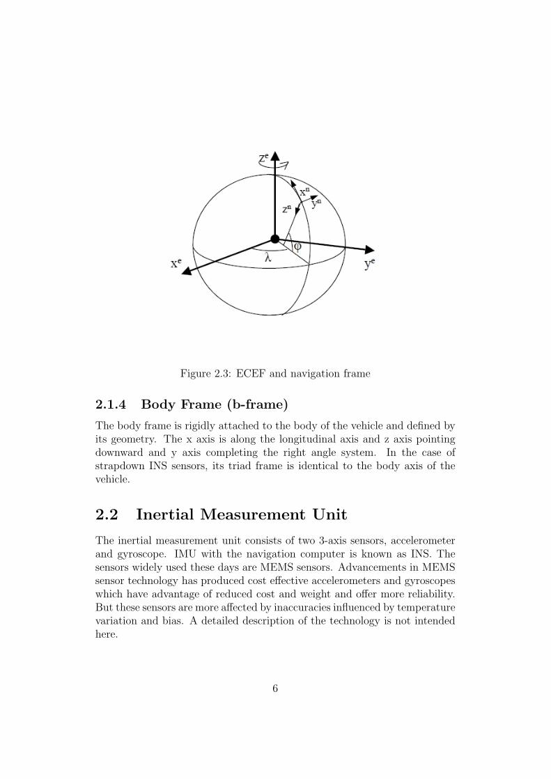
Figure 2.3: ECEF and navigation frame

2.1.4 Body Frame (b-frame)

The body frame is rigidly attached to the body of the vehicle and defined byits geometry. The x axis is along the longitudinal axis and z axis pointingdownward and y axis completing the right angle system. In the case ofstrapdown INS sensors, its triad frame is identical to the body axis of thevehicle.

2.2 Inertial Measurement Unit

The inertial measurement unit consists of two 3-axis sensors, accelerometerand gyroscope. IMU with the navigation computer is known as INS. Thesensors widely used these days are MEMS sensors. Advancements in MEMSsensor technology has produced cost effective accelerometers and gyroscopeswhich have advantage of reduced cost and weight and offer more reliability.But these sensors are more affected by inaccuracies influenced by temperaturevariation and bias. A detailed description of the technology is not intendedhere.

6

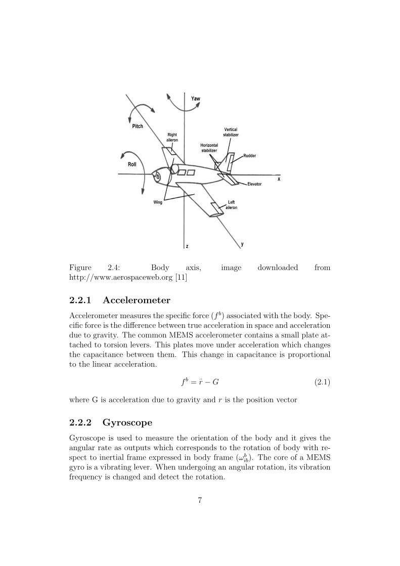
Figure 2.4: Body axis, image downloaded fromhttp://www.aerospaceweb.org [11]

2.2.1 Accelerometer

Accelerometer measures the specific force (f b) associated with the body. Spe-cific force is the difference between true acceleration in space and accelerationdue to gravity. The common MEMS accelerometer contains a small plate at-tached to torsion levers. This plates move under acceleration which changesthe capacitance between them. This change in capacitance is proportionalto the linear acceleration.

f b =..r −G (2.1)

where G is acceleration due to gravity and r is the position vector

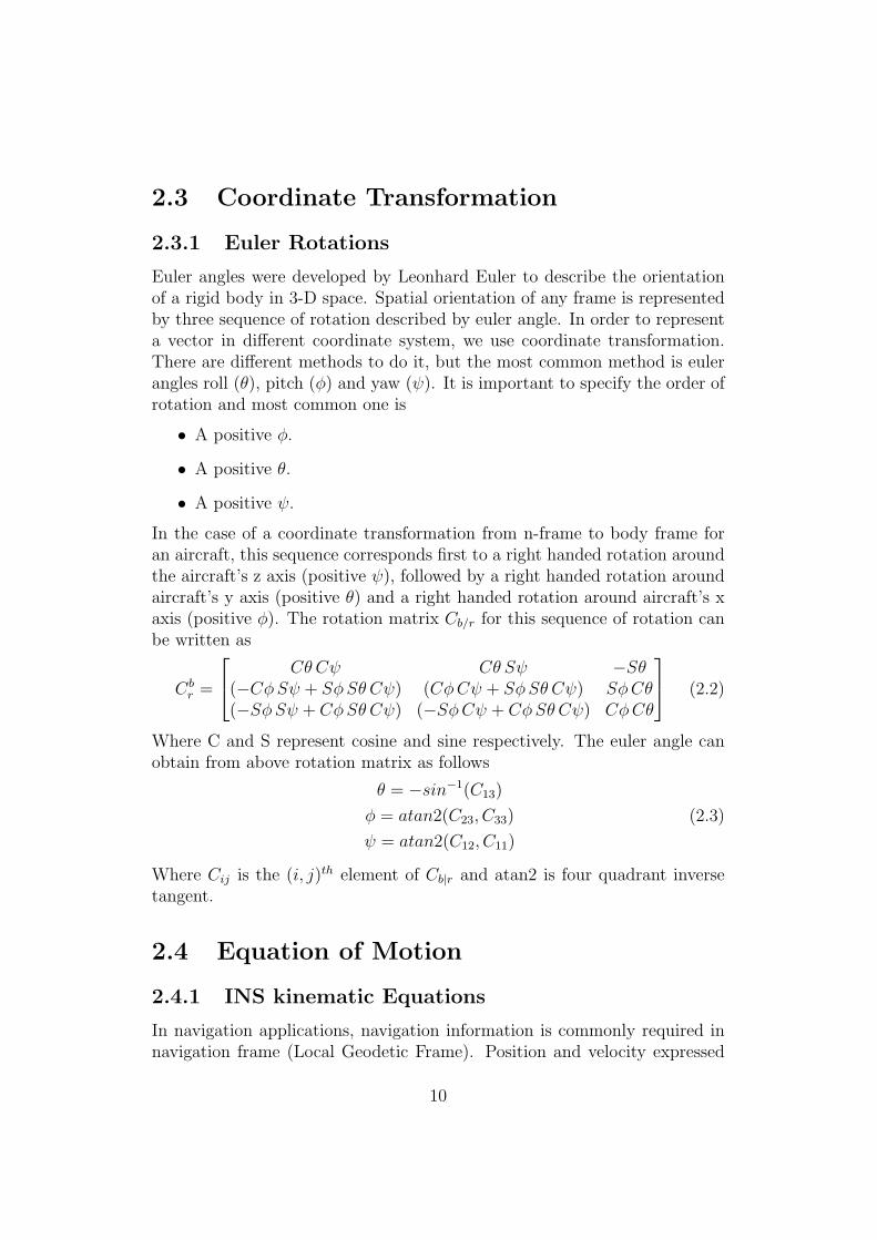
2.2.2 Gyroscope

Gyroscope is used to measure the orientation of the body and it gives theangular rate as outputs which corresponds to the rotation of body with re-spect to inertial frame expressed in body frame (ωbib). The core of a MEMSgyro is a vibrating lever. When undergoing an angular rotation, its vibrationfrequency is changed and detect the rotation.

7

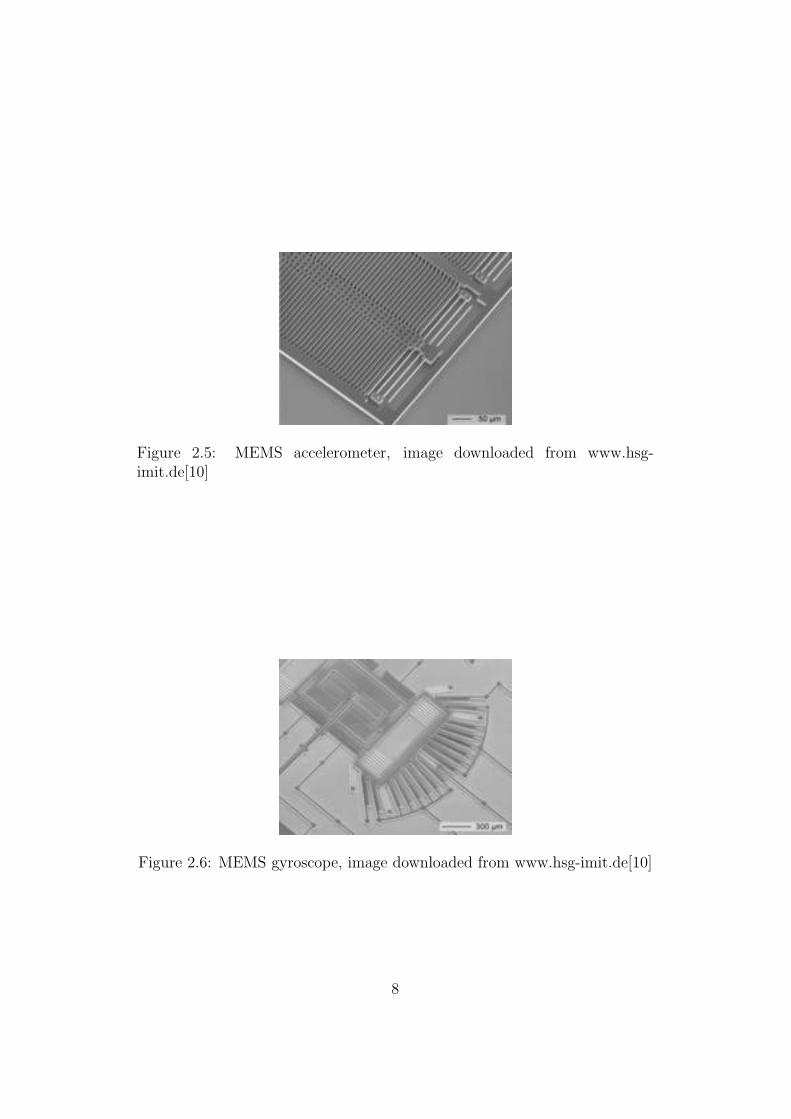
Figure 2.5: MEMS accelerometer, image downloaded from www.hsg-imit.de[10]

Figure 2.6: MEMS gyroscope, image downloaded from www.hsg-imit.de[10]

8

2.2.3 IMU Errors

Below is a brief introduction of some major error sources associated withMEMS sensors.

Accelerometer Bias error

There is some constant offset in accelerometer output which changes slightlyafter each turn on.

Misalignment and Nonorthogonality

The axis of the sensors may be misaligned from the body axis which willproduce an error measurement

Accelerometer Scale Factor error

This error is resulted from the scale factor which is used to convert the valueto common measurement units. This error is proportional to the sensedacceleration.

Gyroscope Drift

The gyroscope drift or bias error results from bias which is a constant offsetfrom correct output but this varies after each turn on of the sensor.

Gyroscope Scale Factor error

This error is proportional to sensed angular rates resulting from variation inthe scale factor of the gyro sensor.

Random Noise

Random noise errors associated with measurements

Nonlinearity due to Temperature variations

The operation of the MEMS technology is affected considerably by temper-ature variations.

9

2.3 Coordinate Transformation

2.3.1 Euler Rotations

Euler angles were developed by Leonhard Euler to describe the orientationof a rigid body in 3-D space. Spatial orientation of any frame is representedby three sequence of rotation described by euler angle. In order to representa vector in different coordinate system, we use coordinate transformation.There are different methods to do it, but the most common method is eulerangles roll (θ), pitch (φ) and yaw (ψ). It is important to specify the order ofrotation and most common one is

• A positive φ.

• A positive θ.

• A positive ψ.

In the case of a coordinate transformation from n-frame to body frame foran aircraft, this sequence corresponds first to a right handed rotation aroundthe aircraft’s z axis (positive ψ), followed by a right handed rotation aroundaircraft’s y axis (positive θ) and a right handed rotation around aircraft’s xaxis (positive φ). The rotation matrix Cb/r for this sequence of rotation canbe written as

Cbr =

Cθ Cψ Cθ Sψ −Sθ(−CφSψ + SφSθ Cψ) (CφCψ + SφSθ Cψ) SφCθ(−SφSψ + CφSθ Cψ) (−SφCψ + CφSθ Cψ) CφCθ

(2.2)

Where C and S represent cosine and sine respectively. The euler angle canobtain from above rotation matrix as follows

θ = −sin−1(C13)

φ = atan2(C23, C33)

ψ = atan2(C12, C11)

(2.3)

Where Cij is the (i, j)th element of Cb|r and atan2 is four quadrant inversetangent.

2.4 Equation of Motion

2.4.1 INS kinematic Equations

In navigation applications, navigation information is commonly required innavigation frame (Local Geodetic Frame). Position and velocity expressed

10

in navigation frame as

rn = [ϕ λ h]T (2.4)

vn = [VN VE VD]T (2.5)

Where ϕ is latitude, λ is longitude, h is altitude, VN is velocity towards north,VE is velocity towards east and VD is velocity towards down. Motion of thevehicle is expressed by the INS kinematic equation or navigation equation.Derivation and more explanation about these equations can be found in manyliteratures, for example in Strapdown Inertial Navigation Technology[4]. Thisequation has 3 parts position, velocity and attitude equations as shown below.

rn =

ϕλh

=

1M+h

0 0

0 1(N+h)cosϕ

0

0 0 −1

VNVEVD

(2.6)

Vn

e = Cnb f

b − (2ωnie + ωnen)× V n + gn (2.7)

Cnb = Cn

b Ωbnb

= Cnb (Ωb

ib − Ωbin)

(2.8)

where M and N are radius of curvature of meridian and prime vertical. Cnb

is the rotation matrix from b-frame to n-frame. g is gravity vector. Ωbnb is

skew symmetric matrix of wbnb and wbnb is equal to wbib −Cbn(wnie +wnen). f b is

the specific force which is the difference between true acceleration in spaceand acceleration due to gravity. ωbib is the output of the gyroscope and ωnie isthe earth rotation rate with respect to inertial frame expressed in navigationframe. ωnen is the rotation rate of the navigation frame with respect to ECEFframe.

2.4.2 INS Mechanization

This section gives a brief explanation about how the INS calculate the nav-igation frame values from the IMU measurements. The inertial navigationsensors measure f b the specific force (accelerometer) and the rotation of body(gyroscope) ωbib. The process of converting this measurements to navigationinformation have mainly 4 steps. (For more about this, please check Adri-ano’s thesis report[22])

• Correction of raw measurement data.

11

• Attitude update ( Cnb )

• Transform specific force into n-frame.

• Velocity and position calculation

Usually the IMU sensors outputs the velocity and angular increments (∆Vb

f

and ∆θb

ib) in body frame for a sampling time period.

Correction of measurement data

The raw measurement data is corrupted by turn on bias, in run bias, scale fac-tor errors and measurement noise. These errors can be measured on groundor it can be estimated during operation. Such measurements can be correctedaccording to the following equations.

∆θbib =

1

(1+Sgx )0 0

0 1(1+Sgy )

0

0 0 1(1+Sgz )

(∆θb

ib − bg∆t) (2.9)

∆V bf =

1

(1+Sax )0 0

0 1(1+Say )

0

0 0 1(1+Saz )

(∆Vb

f − ba∆t) (2.10)

where ba and bg are bias of the accelerometer and gyroscope respectively.Similarly sa and sg are the scale factor errors of the accelerometer and gyro-scope respectively. ∆t is the sampling time.

Attitude update

The Body angular increments with respect to the navigation frame can berepresented as

∆θbnb = [∆θx ∆θy ∆θz]

= ∆θbib − Cbn(ωnie + ωnen)∆t

Cbn = (Cn

b )T(2.11)

The direction cosine matrix (Cnb ) is calculated from the angular increments

using quaternion approach. In quaternion approach, the rotation matrix is

12

expressed by a single rotation angle about a fixed axis. The angular incrementobtained before can be used to update the quaternion vector q as,

qk+1

= qk

+ 0.5

c s∆θz −s∆θy s∆θx

−s∆θz c s∆θx s∆θys∆θy −s∆θx c s∆θz−s∆θx −s∆θy −s∆θz c

qk (2.12)

where

s =2

∆θsin

∆θ

2

c = 2(cos∆θ

2− 1)

∆θ =√

∆θ2x + ∆θ2

y + ∆θ2z

(2.13)

The direction cosine matrix Cnb can finally obtained in terms of quaternion

as

Cbn =

(q20 + q2

1 − q22 − q2

3) 2 (q1 q2 + q0 q3) 2 (q1 q3 − q0 q2)2 (q1 q2 − q0 q3) (q2

0 − q21 + q2

2 − q23) 2 (q2 q3 + q0 q1)

2 (q1 q3 + q0 q2) 2 (q2 q3 − q0 q1) (q20 − q2

1 − q22 + q2

3)

(2.14)

Transformation of specific force into n-frame

For the implementation of the INS equations, specific force needs to convertinto the n-frame. This is done as follows

∆V nf = Cn

b

1 0.5 ∆θz −0.5 ∆θy−0.5 ∆θz 1 −0.5 ∆θx0.5 ∆θy −0.5 ∆θx 1

∆V bf (2.15)

Velocity and position update

The velocity increment in n-frame is obtained by applying the coriolis andgravity correction

∆V n = ∆V nf − (2ωnie + ωnen)× V n∆t+ γn∆t (2.16)

where γn is [0 0 γ]T and γ is the normal gravity at the geodetic latitude ϕand height h. Once the velocity increment is obtained the updated velocityis given by

V nk+1 = V n

k + ∆V nk+1 (2.17)

13

Finally the position in n-frame can be obtained by integrating the velocity

rnk+1 = rnk +1

2D−1 (V n

k + V nk+1) ∆t (2.18)

where

D =

1M+h

0 0

0 1(N+h)cosϕ

0

0 0 −1

(2.19)

Figure 2.7: INS mechanization, image from MSc thesis of Adriano Solimeno[22]

14

Chapter 3

Global Positioning System

This chapter briefly cover the GPS navigation system. Since the implemen-tation considered is loosely coupled, there is not much interest in consideringthe errors or there is no effort to correct for the GPS errors. The informationpresented here is mainly collected from wikipedia[7] and kowoma website[9].

3.1 GPS

The global positioning system is a satellite based navigation system whichwas developed for US military purposes during 70’s and declared completelyoperational in 1995. Generally it has two quality of service, one for militaryand another for civilian purposes. Also they have the option to degrade thequality of the signals whenever and wherever they need, known as “selectiveavailability”. This policy was reconsidered in 2000 and ended the selectiveavailability and gives an accuracy of 100m to 20 m for civilian users.

3.1.1 System Information

The whole GPS system has three components satellites or space segment,control centers (control segment) and GPS receiver modules (user segment).The GPS space segment consists of 24 satellites orbiting in six different or-bital planes (four each in a plane) and completing one rotation in 11 hrs 58minutes. Figure 3.1 gives an approximate idea about the satellite positionand orbits. These planes have an inclination of 55 and are separated by 60right ascension of the ascending node (Fig. 3.2). These satellites have anaverage orbital radius of 20200 km. This arrangement make sure that at leastsix satellites are visible in any point of earth. GPS satellites continually sendnavigation messages at 50 bit/s and main information contained are the time

15

Figure 3.1: Orbits of GPS satellites, image courtesy of kowoma.de

when message was sent, precise orbital information (the ephemeris), and thegeneral system health and rough orbits of all GPS satellites (the almanac).The data format received is usually known as “NMEA” message. The re-ceiver measures the transit time of each message and computes the distanceto each satellite[7]. The control center continuously check the health of thesatellites and do necessary correction when needed. The main monitoringstations are in Hawaii, Kwajalein, Ascension Island, Diego Garcia, ColoradoSprings, Colorado and some other monitor stations operated by the NationalGeospatial-Intelligence Agency. The tracking information is sent to the mas-ter control station. Then mainly two corrections have to perform, the satelliteclocks are synchronized to very high precision and also necessary orbital ma-neuvering have to perform on satellites which are diverted from the correctorbits. During orbital maneuvering, satellite is marked unhealthy and thesignal is excluded by the receiver.

The GPS receivers receive the signals from different satellites and calcu-late the position information. The important components of GPS receiversare antenna, receiver processors and a highly stable clock (crystal oscillator).At least visibility of 4 satellites are necessary for the accurate determinationof the position. In some applications a kalman filter (tightly coupled imple-mentation) can be employed to correct for the errors in the GPS signal. In

16

Figure 3.2: Orbital inclination of GPS satellites, image courtesy ofkowoma.de

the presence of some auxiliary sensors even three satellites can determine theposition well accurately.

3.1.2 Calculation of Position

All satellites broadcast at the same two frequencies, 1.57542 GHz (L1 signal)and 1.2276 GHz (L2 signal)[7]. It employs CDMA technique to transmitthese signal. The low rate message signal is encoded with Pseudo Randomcodes and each satellites has different codes. Two distinct CDMA encodingsare used, the coarse/acquisition (C/A) code (Gold code) and the precise (P)code [7]. The L1 signal employs both C/A and P codes and it’s for thecivilian receivers . L2 employs P codes and it’s meant for military purposes.

GPS receivers use the geometric trilateration to combine the informationfrom different satellite to predict the correct location. The GPS messagecontains the information about the time when message was sent, preciseorbital information, health of the system and rough information regardingthe orbits of other satellites. The receiver measures the time of transit of eachmessage and compute the distance to the satellite. If we know the distancefrom one satellite, we can assume that the receiver is on the surface of a spherecentered by the satellite having the radius equal to the distance. Intersectionof two spheres (if it intersect at more than one point) will be a circle andwhen three spheres intersect result will be two points. Intersection of twospheres is shown in figure 3.3 to have an understanding. We can assumethat the indicated position of the GPS receiver is at the intersection of four

17

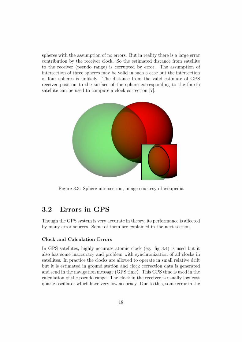
spheres with the assumption of no errors. But in reality there is a large errorcontribution by the receiver clock. So the estimated distance from satelliteto the receiver (pseudo range) is corrupted by error. The assumption ofintersection of three spheres may be valid in such a case but the intersectionof four spheres is unlikely. The distance from the valid estimate of GPSreceiver position to the surface of the sphere corresponding to the fourthsatellite can be used to compute a clock correction [7].

Figure 3.3: Sphere intersection, image courtesy of wikipedia

3.2 Errors in GPS

Though the GPS system is very accurate in theory, its performance is affectedby many error sources. Some of them are explained in the next section.

Clock and Calculation Errors

In GPS satellites, highly accurate atomic clock (eg. fig 3.4) is used but italso has some inaccuracy and problem with synchronization of all clocks insatellites. In practice the clocks are allowed to operate in small relative driftbut it is estimated in ground station and clock correction data is generatedand send in the navigation message (GPS time). This GPS time is used in thecalculation of the pseudo range. The clock in the receiver is usually low costquartz oscillator which have very low accuracy. Due to this, some error in the

18

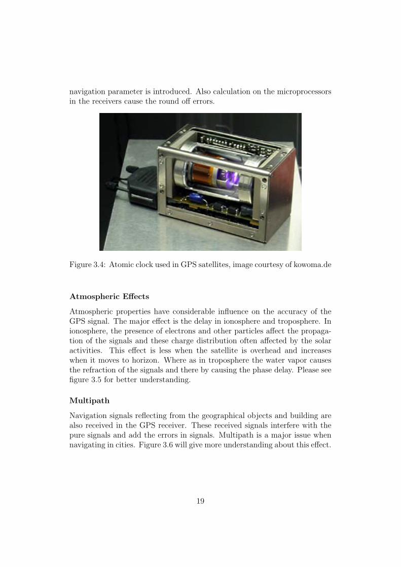
navigation parameter is introduced. Also calculation on the microprocessorsin the receivers cause the round off errors.

Figure 3.4: Atomic clock used in GPS satellites, image courtesy of kowoma.de

Atmospheric Effects

Atmospheric properties have considerable influence on the accuracy of theGPS signal. The major effect is the delay in ionosphere and troposphere. Inionosphere, the presence of electrons and other particles affect the propaga-tion of the signals and these charge distribution often affected by the solaractivities. This effect is less when the satellite is overhead and increaseswhen it moves to horizon. Where as in troposphere the water vapor causesthe refraction of the signals and there by causing the phase delay. Please seefigure 3.5 for better understanding.

Multipath

Navigation signals reflecting from the geographical objects and building arealso received in the GPS receiver. These received signals interfere with thepure signals and add the errors in signals. Multipath is a major issue whennavigating in cities. Figure 3.6 will give more understanding about this effect.

19

Figure 3.5: Effect of atmosphere on GPS signals, image courtesy ofkowoma.de

Figure 3.6: Multipath, image courtesy of kowoma.de

20

Satellite Orbital Errors

Ephemeris data which is transmitted to receiver is calculated from the orbitaldynamics of the satellites. These calculation involve the gravity model andit is a curve fit to the measured data. The trajectory of the satellites can beaffected by many factors like atmosphere and other perturbations. Satellitesalso need constant monitoring and maneuvering to keep the correct trajec-tory.

Relativity

Relativity effects have some contribution to the errors. For example therelativistic time slowing due to the speed of the satellite of about 1 part in1010, the gravitational time dilation that makes a satellite run about 5 partsin 1010 faster than an earth based clock, and the Sagnac effect due to rotationrelative to receivers on earth[7].

Measurement Noise

There is substantial contribution to error by the measurement noise. Thesenoise are created in stages of signal propagation and processing. Some wellknown sources of error are the receiver noise, quantization noise and noisedue to electronics.

Summery of Errors

The errors contributed from some of the major sources are listed as a ta-ble 3.1. These errors added together can accumulate up to ±15 m withoutconsidering the selective availability. With the addition of satellite basedaugmentation system (like WAAS and EGNOS) accuracy can be improvedup to or less than ±5 m. Such systems will compensate for the ionosphericeffects and also improve orbit and clock errors.

21

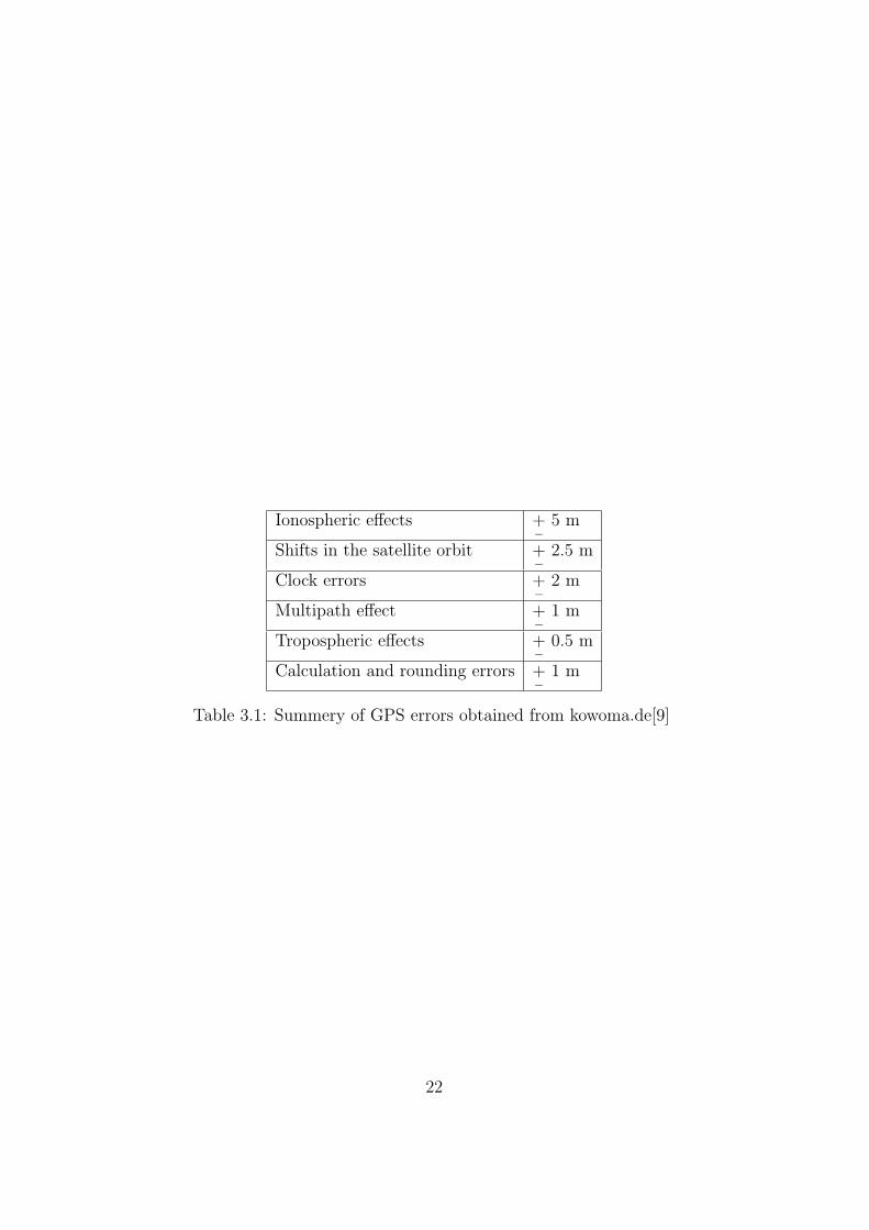
Ionospheric effects +−

5 m

Shifts in the satellite orbit +−

2.5 m

Clock errors +−

2 m

Multipath effect +−

1 m

Tropospheric effects +−

0.5 m

Calculation and rounding errors +−

1 m

Table 3.1: Summery of GPS errors obtained from kowoma.de[9]

22

Chapter 4

Sensor Fusion (KalmanFiltering)

4.1 Introduction to Kalman Filter

The kalman filter is a recursive filter which estimate the states of the dynam-ics of a system by noisy measurement. It was published in 1960 by RudolfE. Kalman and it is now used in many fields of engineering, Economics andScience. It is known as linear quadratic estimator and together with linearquadratic regulator it solves the linear quadratic gaussian control problems[6]. The kalman filter has two distinct steps, prediction and update. Predictor time update step utilize the previous state estimate information to pre-dict the current estimate of state variables. In the second step, also knownas measurement update, the measurement information at current time stepis used to correct the estimate to get more accurate state information

Time Update

Predicted state Xk|k−1 = FkXk−1|k−1 +Bk−1uk−1 (4.1)

Predicted estimate covariance Pk|k−1 = FkPk−1|k−1FTk +Qk−1 (4.2)

Measurement Update

Innovation (residual) covariance Sk = HkPk|k−1HTk +Rk (4.3)

Optimal kalman gain Kk = Pk|k−1HTk S−1k (4.4)

Updated state estimate Xk|k = Xk|k−1 +Kk(Zk −HkXk|k−1)(4.5)

Updated estimate covariance Pk|k = (I −KkHk)Pk|k−1 (4.6)

23

Where Xk|k is the estimate of state at time k given observations up to andincluding time k, K is kalman gain, H is measurement model, Zk is themeasurement at time k, F is state transition matrix, B is input matrix,P is estimate covariance, R is measurement covariance and Q is processcovariance.

4.2 Extended Kalman Filter

The simple kalman filter is applicable only to linear systems. But the realworld problems are usually nonlinear either in process model or in measure-ment model or both. Extended kalman filter is applicable to such problemswith the condition that the process model and measurement model to bedifferential functions of state variables. In EKF, nonlinear state equationand measurement equation are represented as

X(t) = f(X(t), U(t)) + w(t) (4.7)

Zm(t) = h(X(t), U(t)) + v(t) (4.8)

Where f is the nonlinear state equation, h is the nonlinear measurementequation, U is the input vector. w and v represent process and measurementnoise. The above state and measurement nonlinear equations are linearizedabout the prior estimate of the state at each instant of time by calculatingthe Jacobian with respect to the state variables as.

Fk =

(∂f

∂X

); Hk =

(∂h

∂X

); (4.9)

And for discrete time implementation of EKF, the linearized system is dis-cretized in time by computing the system state transition matrix from Fk as[17], where 4t is time interval.

Φk|k−1 = eFk4t ∼= [I + Fk 4 t] (4.10)

The time update and measurement update are as follows.

Time Update

Xk|k−1 = Xk−1|k−1 +

∫ k

k−1

f(X(t), U(t)) dt (4.11)

P k|k−1 = Φk|k−1P k−1ΦTk|k−1 (4.12)

24

The state integration can either done using simple approximation or usingfourth order Runge-Kutta method.

Measurement Update

Sk = HkPk|k−1HTk +Rk (4.13)

Kk = Pk|k−1HTk S−1k (4.14)

Xk|k = Xk|k−1 +Kk(Zk − h(Xk|k−1)) (4.15)

Pk|k = (I −KkHk)Pk|k−1 (4.16)

4.3 Unscented Kalman Filter

The unscented kalman filter was proposed in 1997 as alternative to extendedkalman Filter. When the system become highly nonlinear, ekf is less efficientin estimation. There are two drawbacks in ekf, that it is too difficult totune and only reliable for systems which are almost linear on the time scaleof the update intervals [18]. In this new approach ”Unscented Transform”[20] is used to parameterize mean and covariance which is founded on theintuition that it is easier to approximate a Gaussian distribution than it isto approximate an arbitrary nonlinear function or transformation [18].

4.3.1 Unscented Transform

The unscented transform is a method for calculating the statistics of arandom variable which undergo nonlinear transformation [16]. For exampleconsider a random variable x with dimension L through a nonlinear functiony = f(x), and x has covariance Pxx and mean x. A set of points ”sigmapoints” are chosen such that their mean and covariance are x and Pxx re-spectively. These points are applied in the nonlinear function y = f(x) toget the y and Pyy[18]. It is important to note that the sigma points are notchosen in random but rather according to some deterministic algorithm. Then-dimensional random variable x is approximated by 2L+1 weighted sigmapoints as,

X0 = x

Xi = x+ (√

(L+ λ)Pxx )i , i = 1, ..L

Xi+L = x− (√

(L+ λ)Pxx )i−L , i = L + 1, ..2L

(4.17)

25

Wm0 = λ/(L+ λ)

W c0 = λ/(L+ λ) + (1− α2 + β)

Wmi = W c

i = 1/2(L+ λ) , i = 1, ..2L

(4.18)

Where Wmi and W c

i are the weights of the mean and covariance calculationassociated with ith point. λ = α2(L + k) − L is a scaling parameter and αdetermine the spread of the sigma points around x. k is secondary scalingparameter and β corresponds to the prior knowledge of the distribution of X(for Gaussian distributions, β=2). The default values for these parametersare α = 10−4, β = 2 and k = 3 − L. The method instantiate each sigmapoint through the function y = f(x) resulting in a set of transformed sigmapoints, mean and covariance as

Yi = f(Xi) (4.19)

The mean is given by the weighted average of the transformed points,

y =2L∑i=0

Wmi Yi (4.20)

The covariance is the weighted outer product of the transformed points,

Pyy =2L∑i=0

W ci [Yi − y][Yi − y]T (4.21)

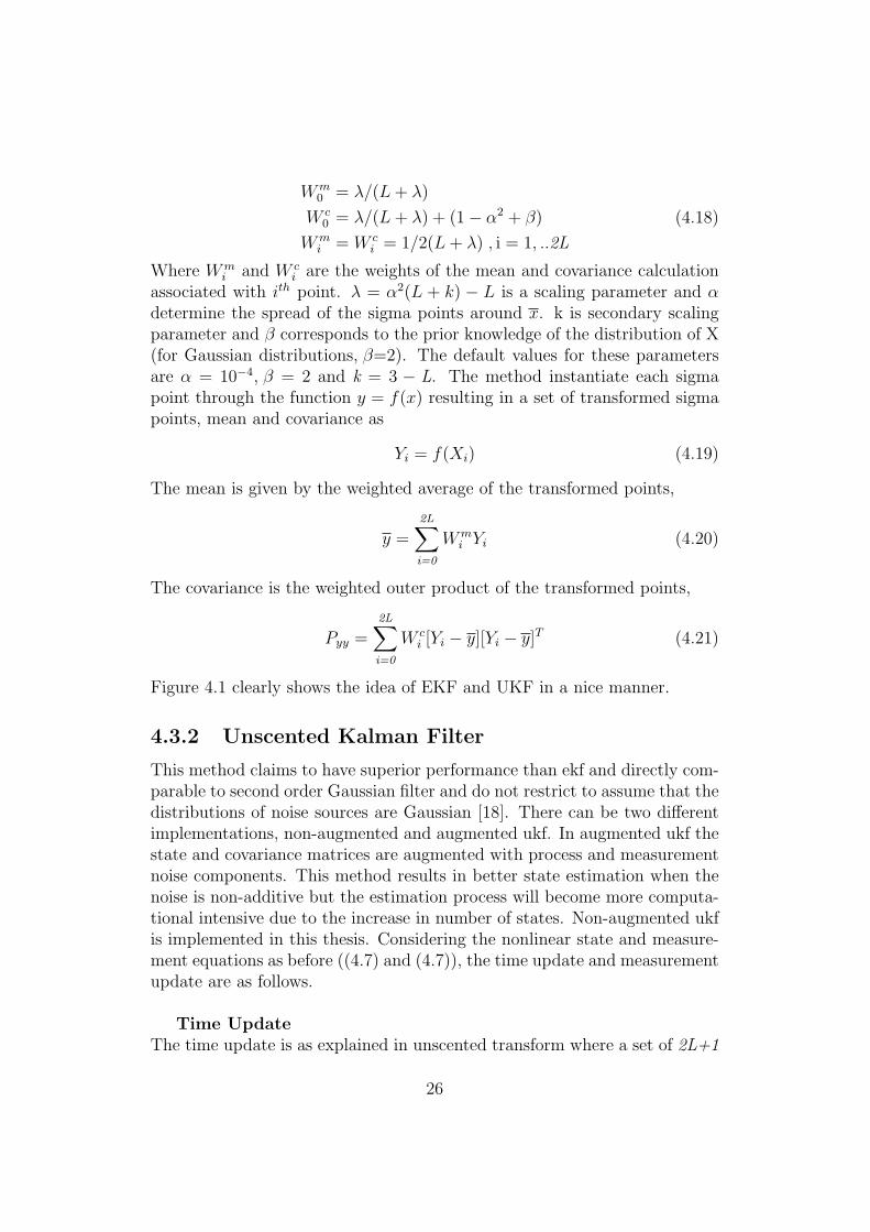
Figure 4.1 clearly shows the idea of EKF and UKF in a nice manner.

4.3.2 Unscented Kalman Filter

This method claims to have superior performance than ekf and directly com-parable to second order Gaussian filter and do not restrict to assume that thedistributions of noise sources are Gaussian [18]. There can be two differentimplementations, non-augmented and augmented ukf. In augmented ukf thestate and covariance matrices are augmented with process and measurementnoise components. This method results in better state estimation when thenoise is non-additive but the estimation process will become more computa-tional intensive due to the increase in number of states. Non-augmented ukfis implemented in this thesis. Considering the nonlinear state and measure-ment equations as before ((4.7) and (4.7)), the time update and measurementupdate are as follows.

Time UpdateThe time update is as explained in unscented transform where a set of 2L+1

26

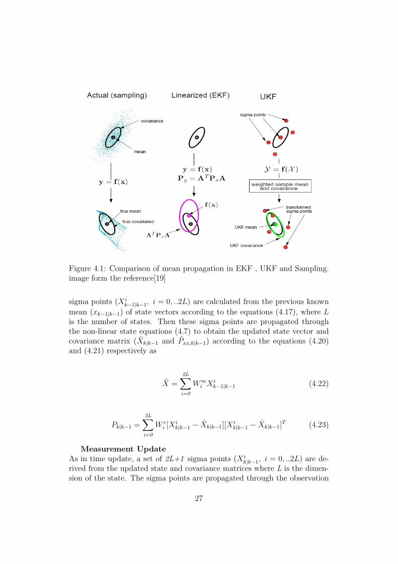
Figure 4.1: Comparison of mean propagation in EKF , UKF and Sampling.image form the reference[19]

sigma points (X ik−1|k−1, i = 0, ..2L) are calculated from the previous known

mean (xk−1|k−1) of state vectors according to the equations (4.17), where Lis the number of states. Then these sigma points are propagated throughthe non-linear state equations (4.7) to obtain the updated state vector andcovariance matrix (Xk|k−1 and Pxx,k|k−1) according to the equations (4.20)and (4.21) respectively as

X =2L∑i=0

Wmi X

ik−1|k−1 (4.22)

Pk|k−1 =2L∑i=0

W ci [X i

k|k−1 − Xk|k−1][Xik|k−1 − Xk|k−1]

T (4.23)

Measurement UpdateAs in time update, a set of 2L+1 sigma points (X i

k|k−1, i = 0, ..2L) are de-rived from the updated state and covariance matrices where L is the dimen-sion of the state. The sigma points are propagated through the observation

27

function h asγik = h

(X ik|k−1

), i = 0, ..2L (4.24)

The predicted measurement and measurement covariance are calculated withweighted sigma points as follows

Zk =2L∑i=0

Wmi γ

ik (4.25)

Pzz,k =2L∑i=0

W ci [γik − Zk][γik − Zk]T (4.26)

The state-measurement cross covariance matrix is obtained as

Pxz,k =2L∑i=0

W ci [X i

k|k−1 − Xk|k−1][γik − Zk]T (4.27)

and ukf kalman gain, updated state and covariance are respectively

Kk = Pxz,k P−1zz,k (4.28)

Xk|k = Xk|k−1 +Kk (Zk − Zk) (4.29)

Pk|k = Pk|k−1 −Kk Pzz,kKTk (4.30)

28

Chapter 5

INS-GPS Integration

5.1 System Process Model for Integration

In ekf implementation of ins-gps integration, the errors of the system mecha-nization is modeled. There are different approaches, proposed by different re-searchers. In all such implementation, idea is to avoid the need of calculatingJacobian necessary for ekf by simplifying the error equations using differentapproximations and assumptions. But when the errors are very large, thesemethods fail to give a reasonable estimation. Also problems with the initialerrors and alignment. In ukf implementation the mechanization equationitself is considered for implementation. To utilize the full potential of ukfalgorithm, mechanization equations explained in section 2.4.1 ((2.6), (2.7),(2.8)) need to consider. The state of the system is augmented by adding biasand scale factor errors as state variables.

5.2 Sensor Modeling

The INS sensors used in this study are of MEMS technology. The noisesources considered here in modeling are bias errors, scale factor errors andwhite random noise.

5.2.1 Inertial sensor error models

The measurement equation for accelerometer and gyroscope can be writtenas follows

29

fb

= f b + ba + diag(f b)Sa + wa (5.1)

ωbib = ωbib + bg + diag(ωbib)Sg + ωg (5.2)

where fb

is the measured accelerometer value and f b is the true value.

ωbib is the measured gyroscope value and ωbib is the true value. ba and bg arethe biases of accelerometer and gyroscope respectively. Sg and Sa are scalefactor errors of gyroscope and accelerometer.

The bias error of low cost MEMS sensors are sum of a constant bias(turn-on bias) plus a non constant variation (in-run bias)

b(t) = btob(t) + δb(t) (5.3)

where btob is turn on bias and δb(t) is the in-run bias drift. The randomconstant although being constant, can vary on each turn on. So the bestmodel is the random constant.

.

b(t) = 0 (5.4)

The in-run bias can be modeled as first order Gauss-Markov process.

δ.

b(t) = − 1

Tbδb(t) + wb(t) (5.5)

The scale factor error is usually a constant but for MEMS sensors it can varywith time so it is also modeled as first order Gauss-Markov process as

δ.

S(t) = − 1

TSδS(t) + wS(t) (5.6)

The random noise is modeled as zero mean white Gaussian noise.

5.3 Measurement Equations

The equations for measurement update can be summarized as follows. ThoughGPS can be considered as very accurate, it is still affected by some errors. Itis modeled as white Gaussian noise. Finally all the measurement equations

30

are given below.

fb

= f b + ba + diag(f b)Sa + wa

ωbib = ωbib + bg + diag(ωbib)Sg + ωg

ϕgps = ϕ+ wϕ

λgps = λ+ wλ

hgps = h+ wh

VN,gps = VN + wVN

VE,gps = VE + wVE

VD,gps = VD + wVD

(5.7)

The variables ϕgps, λgps, hgps, VN,gps, VE,gps and VD,gps are the correspondingmeasured values from GPS unit and w is white Gaussian noise.

31

Chapter 6

Implementation in Matlab

Unscented kalman filter algorithm was implemented and simulated usingmatlab. AeroSim an aeronautical simulation block set was utilized for gen-erating the trajectory.

6.1 Trajectory Generator

In order to simulate the algorithms, one proper trajectory was necessary.Freely available aeronautical simulation blockset from Unmanned Dynam-ics (AeroSim-blockset) was employed to generate the trajectory of an air-craft. This toolbox can be downloaded for academic and non-commercialuse for free of charge [13]. According to their website, AeroSim blockset is aMatlab/Simulink block library which provides components for rapid devel-opment of nonlinear 6-DOF aircraft dynamic models. In addition to aircraftdynamics the block set also includes environment models such as standardatmosphere, background wind, turbulence and earth models (geoid reference,gravity and magnetic field). This block set currently only works under win-dows operating system. Some of the features they claim are

• Full 6-DOF simulation of nonlinear aircraft dynamics

• Visual output to Microsoft Flight Simulator and FlightGear Flight Sim-ulator

• Complete aircraft models that can be customized via parameter files

• Sample aircraft models including the Aerosonde UAV and the NorthAmerican Navion

• Ability to automatically generate C code from Simulink aircraft modelsusing Real-Time Workshop.

32

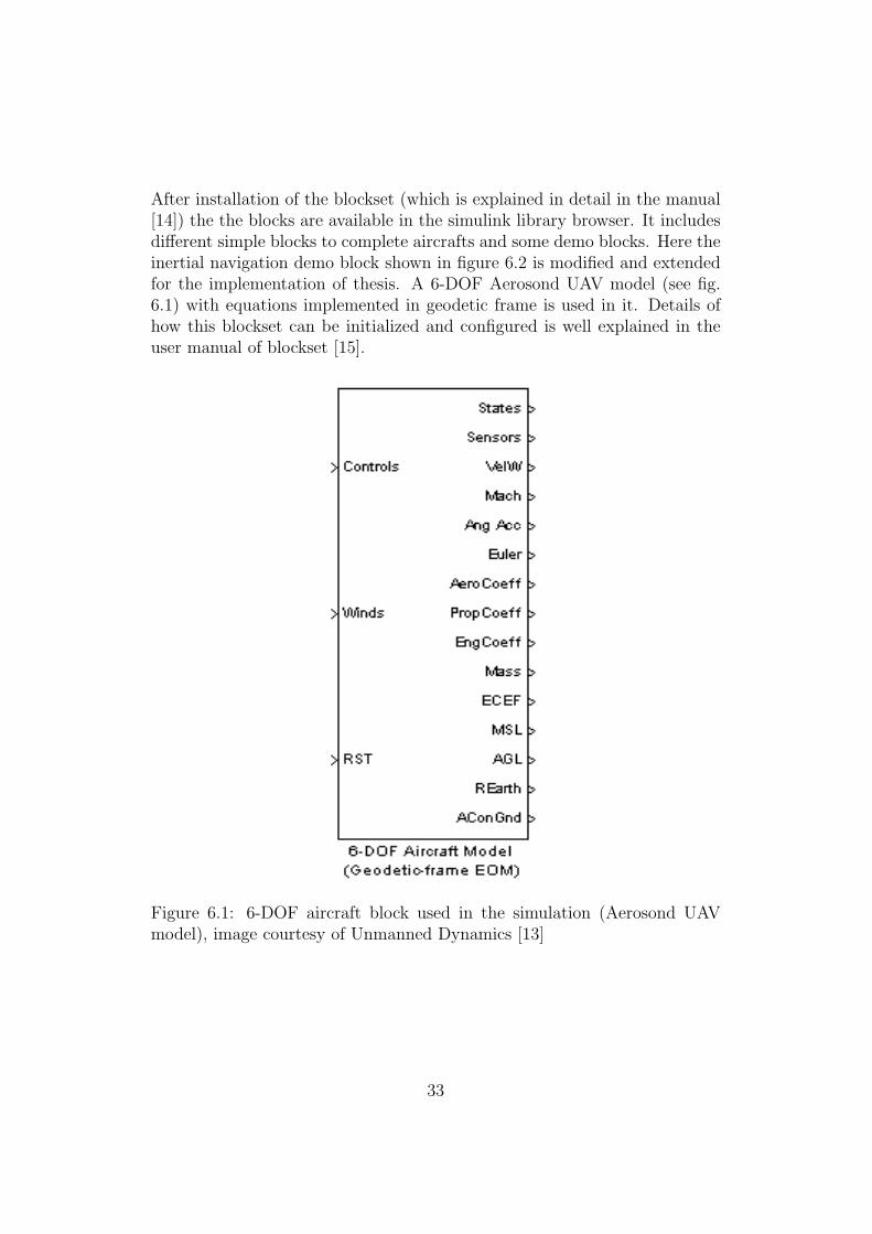
After installation of the blockset (which is explained in detail in the manual[14]) the the blocks are available in the simulink library browser. It includesdifferent simple blocks to complete aircrafts and some demo blocks. Here theinertial navigation demo block shown in figure 6.2 is modified and extendedfor the implementation of thesis. A 6-DOF Aerosond UAV model (see fig.6.1) with equations implemented in geodetic frame is used in it. Details ofhow this blockset can be initialized and configured is well explained in theuser manual of blockset [15].

Figure 6.1: 6-DOF aircraft block used in the simulation (Aerosond UAVmodel), image courtesy of Unmanned Dynamics [13]

33

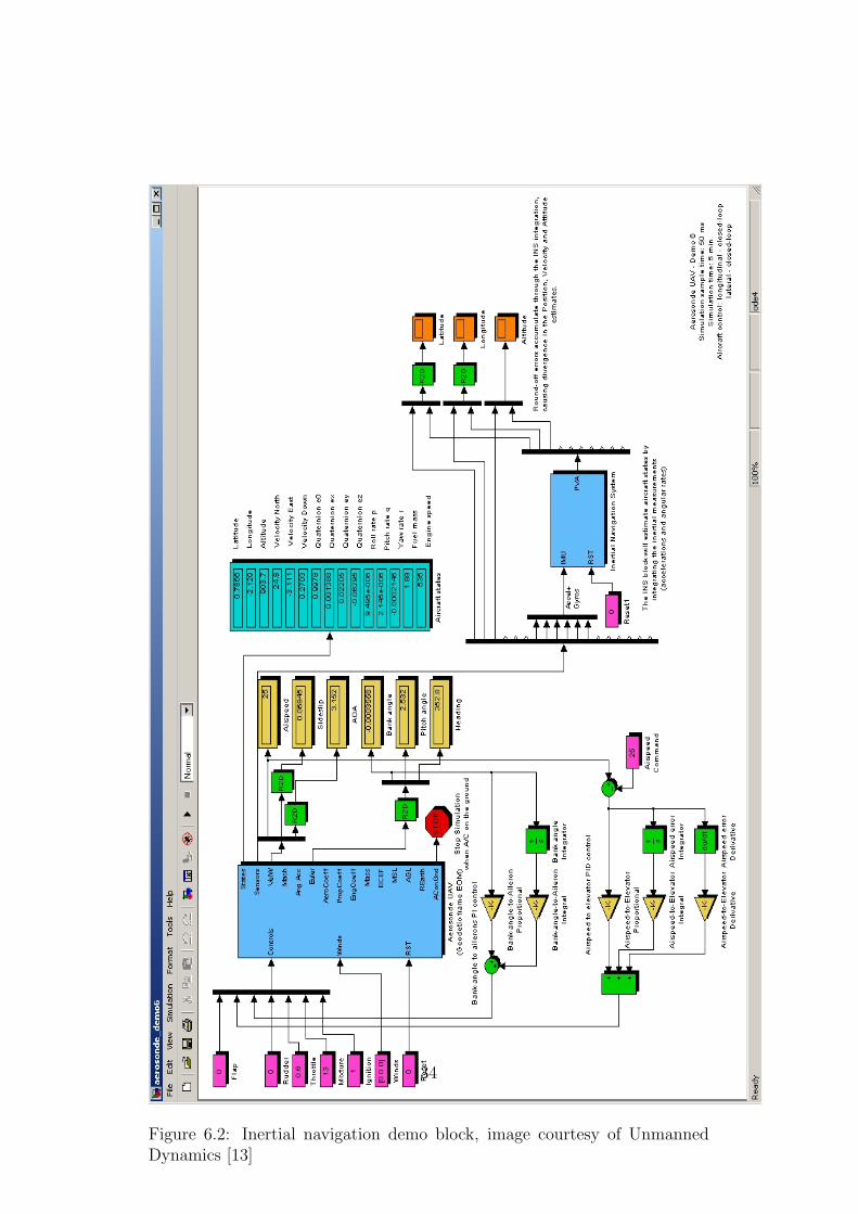
Figure 6.2: Inertial navigation demo block, image courtesy of UnmannedDynamics [13]

34

6.2 Software for UKF Implementation

There are some useful packages and blocksets available from different sourcesfor implementation of Kalman filters and smoothers. The ReBEL toolkit isone of such toolkit available from the OGI School of Science and Engineering,Oregon Health and Science University. They claim it is free for academic use.Another useful toolbox, EKF/UKF toolbox for matlab from Department ofBiomedical Engineering and Computational Science (BECS), Center of Ex-cellence in Computational Complex Systems Research, Helsinki Universityof Technology is available from their homepage [25]. In this thesis for imple-mentation of ukf, the functions available from this toolbox is used in greaterextend but I have modified some of the matlab files for more convenience inmy implementations. Also there are a number of good examples implemen-tations along with this blockset. Interestingly the Reentry Vehicle Trackingproblem which was used (Julier and Uhlmann [18]) to demonstrate the per-formance of UKF is also implemented and included as demonstration.

6.3 INS-GPS Integration Implementation

The state vectors are ϕ, λ , h, VN , VE, VD , q0, q1, q2, q3, bax , bay , baz , bgx ,bgy , bgz , Sax , Say , Saz , Sgx , Sgy , Sgz . There are 22 state variables in this pro-posed implementation. They are composed of position, velocity, quaternion,bias of sensors and scale factor of sensors as noted above. Non-augmentedukf implementation is performed here. Suitable initial conditions are set forthe states. Other variables needed for the operation of the blocks are setusing initialization file. In order to generate the trajectory and sensor data,simulink Aerosond UAV model is simulated with suitable initial conditions.To choose a particular trajectory the control inputs (rudder, throttle etc.)and environmental constraints are applied to the model. The UAV modeloutputs the sensor data which is used in later stage for filter implementationand comparison. One set of measurement data is passed to the unaided INSmodule which will generate the uncompensated output. Other set of data ispassed over to the aided INS block and ukf filter implementation for estima-tion. Figure 6.3 shows the ins-gps integration implementation and figure 6.5shows in more detail about how estimated values are applied in correction ofnavigation information. Figure 6.4 shows the INS error modeling in simulink.

35

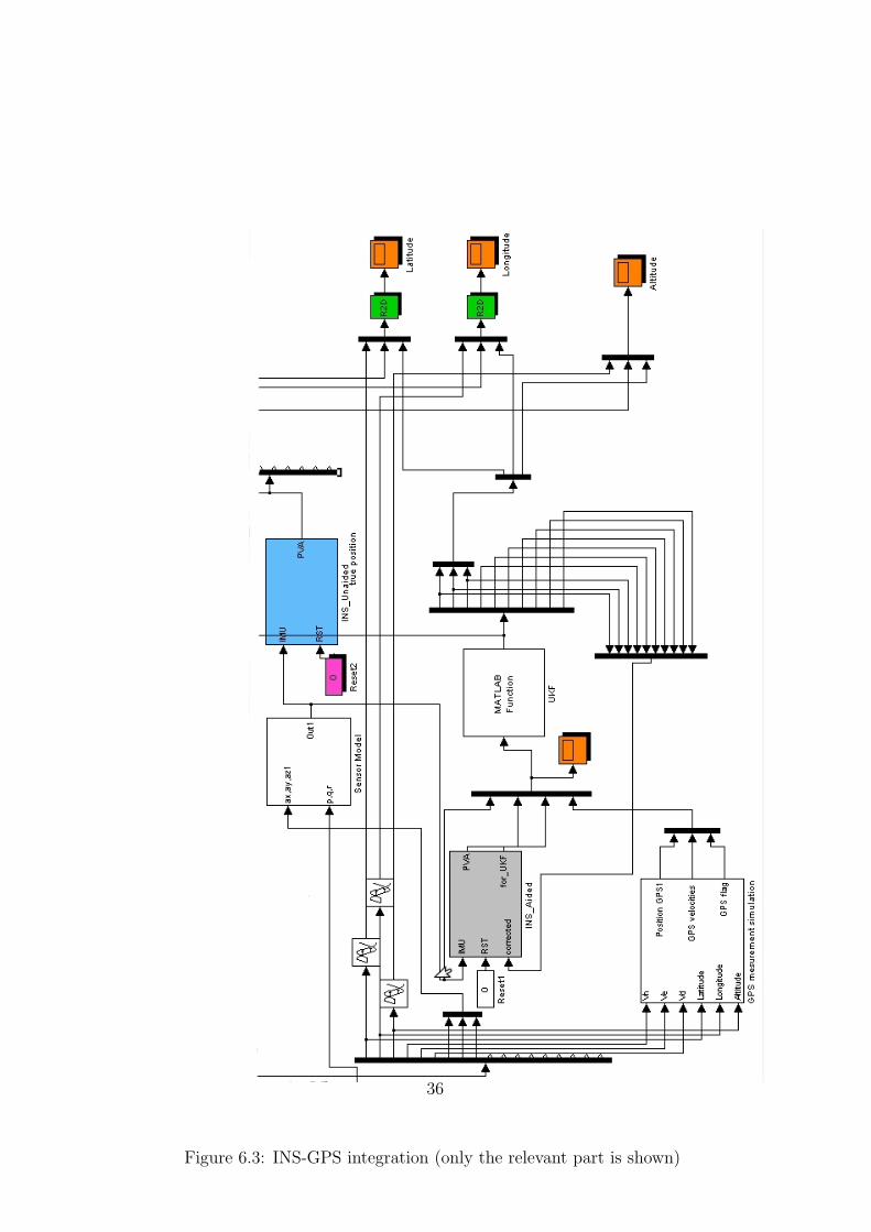
Figure 6.3: INS-GPS integration (only the relevant part is shown)

36

Figure 6.4: INS error model

37

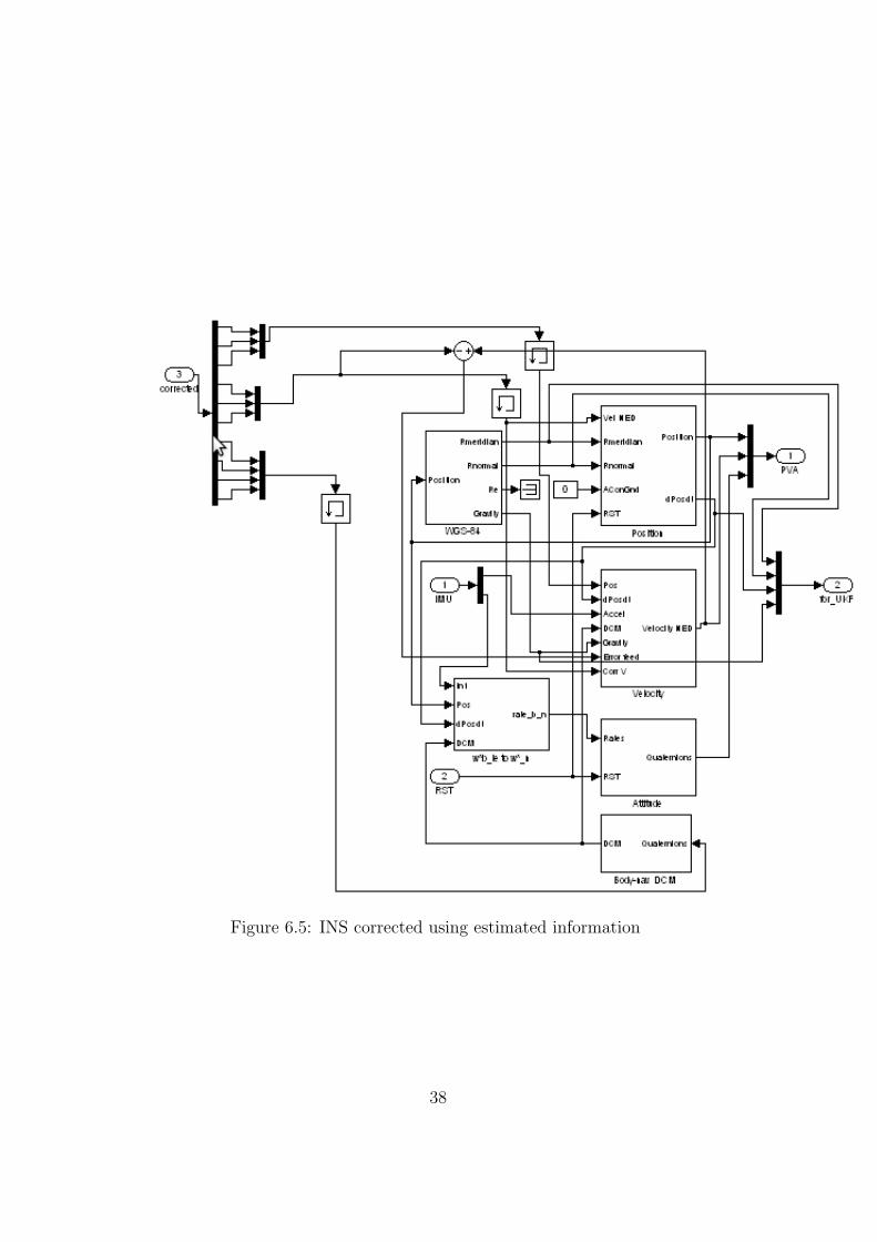
Figure 6.5: INS corrected using estimated information

38

In the original implementation in Aerosim blockset, the sensor outputfrom gyroscope was the rate of the body with respect to the navigationframe (ωbn), but the gyroscope measurement is with respect to inertial frame.INS block was implemented to use this value to generate the navigation in-formation. So model is modified to get the correct gyro output and then INSblock is also modified according to that. Figure 6.7 shows the modificationand figure 6.6 shows the original INS implementation.

Figure 6.6: INS block, aerosim

39

Figure 6.7: INS block, modified

40

6.4 Attitude Estimation Implementation

An attitude estimation problem explained in [1] (of a stabilized platform)was considered finally due to the difficulties faced with INS-GPS integrationand also due to time constraints. The main difficulties were the instabilityof cholesky factorization implementation “chol“ and availability of trajectorygenerator. Sensors used in this implementation are 3-axis accelerometer, gy-roscope and magnetometer. Here is a brief problem description and equationsused in the filtering implementation.

6.4.1 Kinematic Equation in Quaternion

The kinematic equation of rigid body motion is derived as follows in theliterature [3] and is widely used in digital navigation processing. Analogous tothe euler kinematic equation, let Fr be a reference frame and Fb be a rotatingframe and orientation at any time ’t’ can be represented in quaternion asqb|r(t). Let the instantaneous angular velocity of Fb along a unit vector k bew, then in δt interval δqb|r can be approximated as

δqb|r(δt) ≈[

1

k wδt/2

](6.1)

and finally the derivative of quaternion is obtained as

q =1

2qb|r ∗ wbb|r (6.2)

Where ’*’ is quaternion multiplication and wbb|r is the angular velocity of bframe with respect to r frame expressed in b frame. And in matrix form

q0q1q2q3

= 1/2

0 −P −Q −RP 0 R −QQ −R 0 PR −Q −P 0

q0q1q2q3

(6.3)

Here P, Q and R are angular velocities in body axis and q0, q1, q2, q3 are com-ponents of quaternion. These equations are the basics of attitude estimationimplementation in digital navigation aids.

6.4.2 Sensor Modeling

For attitude estimation of stabilized platform, the sensors used are 3-axisaccelerometers, gyroscope and magnetometer. The sensor errors considered

41

are temperature drift, CG offset, bias and random noise. The bias errors(both in accelerometer, gyroscope and magnetometer) are considered as statevariables. The accelerometer is modeled as

AxAyAz

measured

=

AxAyAz

true

+

− 0.0056T + 0.0430.00056 − 0.0023T + 0.000143

0.034 − 0.0096T + 0.0073

+

−(q2 + r2)XAx

−(p2 + r2)XAy

−(p2 + q2)XAz

+

BAx

BAy

BAz

(6.4)

And gyroscope is modeled as followspqr

measured

=

pqr

true

+

− 0.0065T 3 + 0.0045T 2 − 0.0026T + 0.0530.00056T 2 − 0.000823T + 0.000543

0.000037T 3 + 0.014T 2 − 0.0094T + 0.000373

+

Bpx

Bqy

Brz

(6.5)

Where −(q2 + r2)XAx

−(p2 + r2)XAy

−(p2 + q2)XAz

(6.6)

accounts for the CG offset error. Ax, Ay and Az are the accelerometer values.p, q and r are the gyroscope values and they are angular rates in body frame.XAx , XAy and XAz are the CG offset of accelerometer. T is temperature andB is corresponding bias value. The temperature drift is not estimated butjust corrected before the estimation and in real situation the temperaturesensor is used to get the accurate temperature which will be used for abovetemperature drift calibration. Constant bias error is considered in all sensorsand the random noise is white Gaussian noise.

6.4.3 Matlab Implementation

For simulation, the sensor measurement data was generated using simulinkblocks. The simulink blocks are shown in figures 6.8, 6.9 and 6.10. The statemodel consists of 15 state variables including four quaternion and the biasof each sensors. Quaternion was used in the implementations because of itsadvantages over euler angles.

42

The state model is

q0 =1

2(−q1 p− q2 q − q3 r)

q1 =1

2(−q0 p+ q2 r − q3 q)

q2 =1

2(−q0 q − q1 r + q3 p)

q3 =1

2(−q0 r + q1 q − q2 p)

p = −1

τp

q = −1

τq

r = −1

τr

Bp = 0

Bq = 0

Br = 0

BAx = 0

BAy = 0

BAz = 0

BHx = 0

BHy = 0

(6.7)

where τ is time constant

The measurement model is

1 = (q20 + q2

1 + q22 + q2

3)

Ax,m = Ax1 +BAx + wAx

Ay,m = Ay1 +BAy + wAy

Az,m = Az1 +BAz + wAz

Hx,m = Hbx +BHx + wHx

Hy,m = Hby +BHy + wHy

(6.8)

43

whereAx1

Ay1Az1

=

AbxAbyAbz

−(q2 + r2)XAx

(p2 + r2)XAy

(p2 + q2)XAz

− − 0.0056T + 0.043

0.00056 − 0.0023T + 0.0001430.034 − 0.0096T + 0.0073

(6.9)

and

AbxAbyAbz

=

(q20 + q2

1 − q22 − q2

3) 2(q1q2 + q0q3) 2(q1q3 − q0q2)2(q1q2 − q0q3) (q2

0 − q21 + q2

2 − q23) 2(q2q3 + q0q1)

2(q1q3 + q0q2) 2(q2q3 − q0q1) (q20 − q2

1 − q22 + q2

3)

Agx

Agy

Agz

(6.10)

[Hbx

Hby

]=

(q20 + q2

1 − q22 − q2

3) 2(q1q2 + q0q3) 2(q1q3 − q0q2)2(q1q2 − q0q3) (q2

0 − q21 + q2

2 − q23) 2(q2q3 + q0q1)

2(q1q3 + q0q2) 2(q2q3 − q0q1) (q20 − q2

1 − q22 + q2

3)

Hgx

Hgy

Hgz

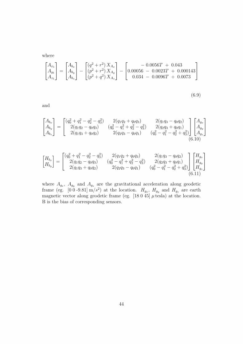
(6.11)

where Agx , Agy and Agz are the gravitational acceleration along geodeticframe (eg. [0 0 -9.81] m/s2) at the location. Hgx , Hgy and Hgz are earthmagnetic vector along geodetic frame (eg. [18 0 45] µ tesla) at the location.B is the bias of corresponding sensors.

44

Figure 6.8: Data generation simulink block, attitude estimation

45

Figure 6.9: Data generation in detail

46

Figure 6.10: Sensor modeling

47

Chapter 7

Results

The main objectives of the thesis were to compare the computational require-ments of both algorithm and then the performance of the filter with differentinitial errors. Ins-gps integration implementation faced different difficultiesand needed more time, so an attitude estimation problem was finally consid-ered. Please note that the objectives of the thesis were achieved with thisattitude estimation problem. Both extended and unscented implementationwere done using matlabR2007b in a Lenovo 32-bit Dual Core laptop. Systemconfiguration is given in table 7.1.

The main difficulty faced in tuning ukf filter was the instability of ‘chol’decomposition which was used as an approximation for calculating squareroot of P matrix. When if the R and Q matrix are not chosen properly,the algorithm will fail in the first step or after a few iterations. This madeit difficult to tune the filter. By observation the step where the instabilityoccurs was found to be at (4.23) in time update where process covarianceprediction is done. This is the step where the P matrix becomes negativedefinite for the first time. Below is the detailed discussion of the resultsobtained from implementations.

48

System ConfigurationOperating System Ubuntu Release 9.04, Kernel Linux 2.6.28-

11-generic, GNOME 2.26.1Hardware Configuration Dual Core Processor, Processor 0: Genuine

Intel(R) CPU T2080@1.73GHz, Processor 1:Genuine Intel(R) CPU T2080@1.73GHz

Software Tool used for simulation Matlab R2007b

Table 7.1: System Configuration for Simulations

Figure 7.1: Snap of system monitor during EKF algorithm execution

Figure 7.2: Snap of system monitor during UKF algorithm execution

49

CPU time usedEKF UKF

CPU time used for processing of data (3500data samples)

.77s 31.64s

CPU time used for single time update step 2.59× 10−04s 56× 10−04sCPU time used for single measurement up-date step

4.42× 10−04s 52× 10−04s

Table 7.2: Comparison of computational resources utilized

7.1 UKF Vs EKF

In order to compare the performance of the ukf and ekf, estimation ofattitudes (roll, pitch and yaw) of stabilized platform in both implementationswere considered. Different aspects of filters were considered, such as sum ofsquares of difference of filtered values to the true attitude values, systemresources like CPU time used and performance with initial errors. Theseresults are summarized in tables.

Table 7.2 compares the CPU time used by both implementations. Alsofigures 7.1 and 7.2 are the snaps of the system monitor window during exe-cution of ekf and ukf implementations respectively. The CPU time used byekf and ukf are found to be .77 seconds and 31.64 seconds respectively. For asingle prediction step in ekf and ukf, the average time used was 2.59× 10−04

and 56×10−04 seconds respectively. Where as the measurement update took4.42 × 10−04 and 52 × 10−04 seconds respectively. Table 7.3 gives the sumof squares comparison of both ukf and ekf implementations. The figures 7.3,7.4 and 7.5 are from the corresponding ekf implementation results and fig-ures 7.6, 7.7 and 7.8 are from ukf implementation results. Though it is notclear from the graphs, when considering the sum of squares of first 500 datasamples, it is clear that ukf has less variation from reality in the beginning.It is also clear from the figures 7.5 and 7.8 that estimation of psi angle isworse in ekf implementation but better in ukf.

50

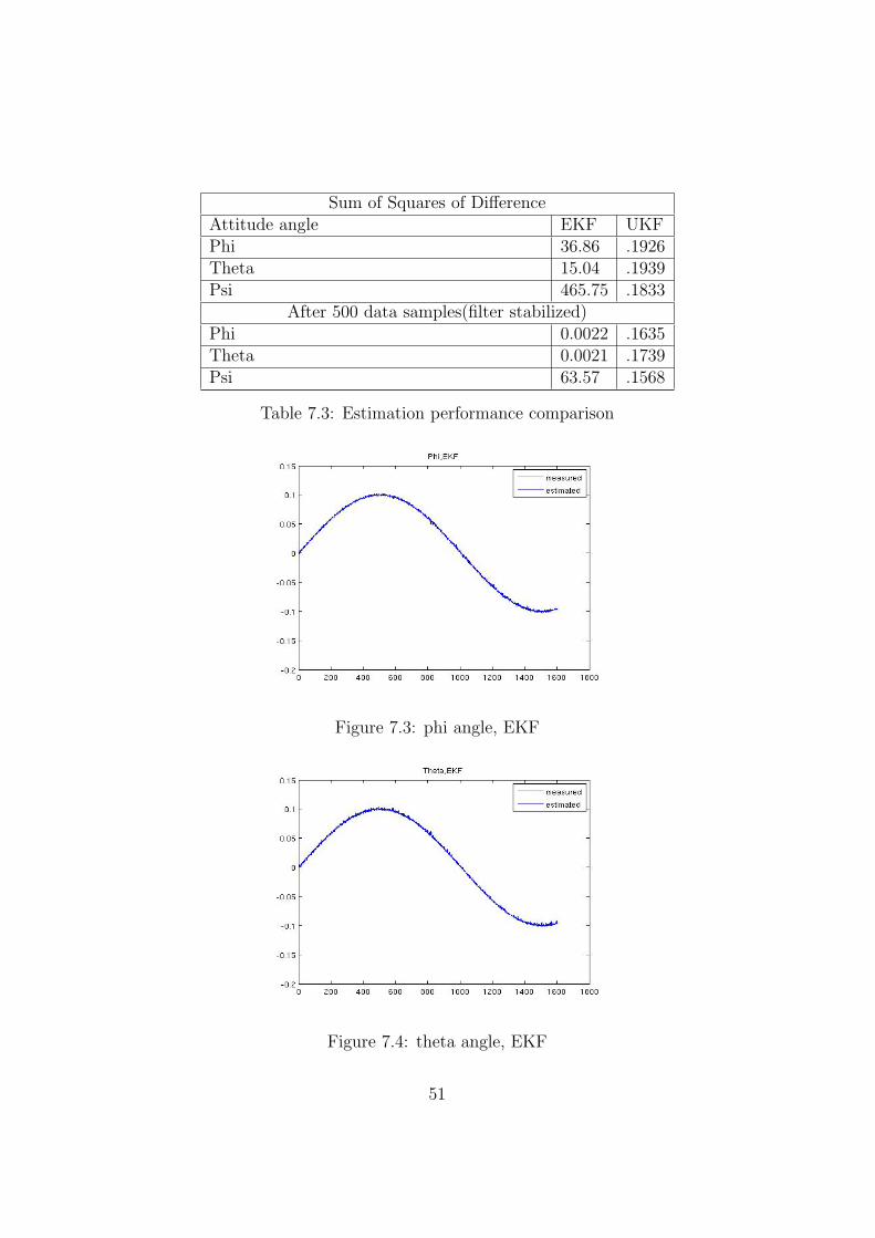
Sum of Squares of DifferenceAttitude angle EKF UKFPhi 36.86 .1926Theta 15.04 .1939Psi 465.75 .1833

After 500 data samples(filter stabilized)Phi 0.0022 .1635Theta 0.0021 .1739Psi 63.57 .1568

Table 7.3: Estimation performance comparison

Figure 7.3: phi angle, EKF

Figure 7.4: theta angle, EKF

51

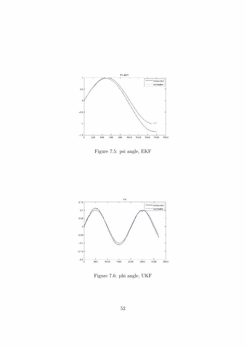
Figure 7.5: psi angle, EKF

Figure 7.6: phi angle, UKF

52

Figure 7.7: theta angle, UKF

Figure 7.8: psi angle, UKF

53

In order to test the performance of the filter with different initial errors,three different set of initial conditions are applied with more variation fromfirst set to third set. The results of sum of squares of difference are presentedas tables 7.4 and 7.5 for ekf and ukf respectively. The values for first 200data samples and complete samples are separately shown to understand theperformance in the initial stage of estimation. It is seen that the ukf attainstability before ekf when the initial conditions are more away from reality.Also estimation of psi angle (see figure 7.9) in ekf was degraded considerablywith increasing initial errors but ukf has a good result (see figure 7.10).The figures 7.11 and 7.12 are results of ekf implementation with second set(medium errors) of initial values. The figures 7.13 and 7.14 are results ofekf implementation with third set (larger errors) of initial values. It is clearform comparing theses two graphs that as initial error increase, ekf estimationtakes more time to stabilize. The figure 7.15 is result of ukf implementationwith third set (larger errors) of initial values and it is not affected much bythe initial errors. In order to enhance the understanding of results, residuals(difference between actual and estimated values) are plotted for simulationswith different set of initial errors. Figures 7.16, 7.17 and 7.18 are residualplots with smaller initial errors. Figures 7.19, 7.20 and 7.21 are residual plotswith medium initial errors. Figures 7.22, 7.23 and 7.24 are residual plots withlarger initial errors. The ekf has more variations in the beginning, but bothalgorithms have similar performance in a long run.

Figure 7.9: psi angle, ekf with third set (larger errors) of initial values

54

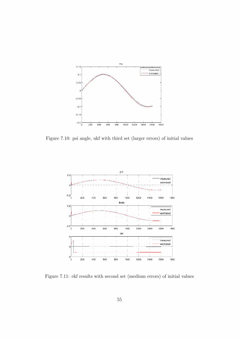
Figure 7.10: psi angle, ukf with third set (larger errors) of initial values

Figure 7.11: ekf results with second set (medium errors) of initial values

55

Figure 7.12: First 200 data samples of ekf results with second set (mediumerrors) of initial values

Figure 7.13: ekf results with third set (larger errors) of initial values

56

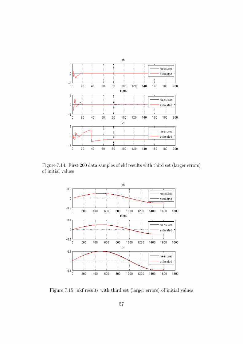
Figure 7.14: First 200 data samples of ekf results with third set (larger errors)of initial values

Figure 7.15: ukf results with third set (larger errors) of initial values

57

Figure 7.16: Residual of phi angle estimate with small initial errors (first 200data samples)

Figure 7.17: Residual of theta angle estimate with small initial errors (first200 data samples)

58

Figure 7.18: Residual of psi angle estimate with small initial errors (first 200data samples)

Figure 7.19: Residual of phi angle estimate with medium initial errors (first200 data samples)

59

Figure 7.20: Residual of theta angle estimate with medium initial errors (first200 data samples)

Figure 7.21: Residual of psi angle estimate with medium initial errors (first200 data samples)

60

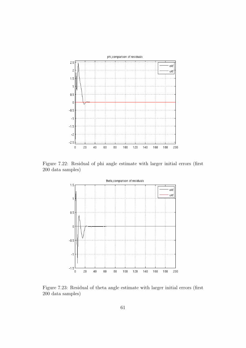
Figure 7.22: Residual of phi angle estimate with larger initial errors (first200 data samples)

Figure 7.23: Residual of theta angle estimate with larger initial errors (first200 data samples)

61

Figure 7.24: Residual of psi angle estimate with larger initial errors (first 200data samples)

62

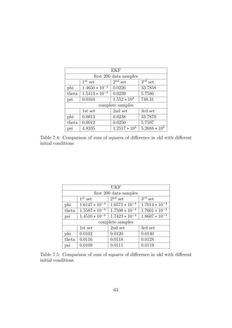
EKFfirst 200 data samples

1st set 2nd set 3rd setphi 1.4650 ∗ 10−4 0.0226 33.7858theta 1.5413 ∗ 10−4 0.0239 5.7586psi 0.0164 1.552 ∗ 103 748.31

complete samples1st set 2nd set 3rd set

phi 0.0013 0.0238 33.7870theta 0.0012 0.0250 5.7597psi 4.8335 1.2517 ∗ 104 5.2688 ∗ 103

Table 7.4: Comparison of sum of squares of difference in ekf with differentinitial conditions

UKFfirst 200 data samples

1st set 2nd set 3rd setphi 1.6147 ∗ 10−4 1.6571 ∗ 10−4 1.7014 ∗ 10−4

theta 1.5587 ∗ 10−4 1.7598 ∗ 10−4 1.7601 ∗ 10−4

psi 1.4510 ∗ 10−4 1.7423 ∗ 10−4 1.8607 ∗ 10−4

complete samples1st set 2nd set 3rd set

phi 0.0102 0.0120 0.0140theta 0.0116 0.0118 0.0128psi 0.0109 0.0111 0.0119

Table 7.5: Comparison of sum of squares of difference in ukf with differentinitial conditions

63

7.2 INS-GPS Integration Results

Because of the lack of time, the complete tuning of the UKF filter for INS-GPS integration had to stop in the middle. Some available results so far isadded below. Figures 7.25, 7.26 and 7.27 are results of estimation of latitudelongitude and altitude respectively. Both implementation and tuning of thefilter have to be improved from the current state and so far no considerableresult is obtained.

Figure 7.25: latitude

64

Figure 7.26: longitude

Figure 7.27: altitude

65

Chapter 8

Conclusion

Attitude estimation of a stabilized platform is studied and implemented tocompare ekf and ukf. The original plan of implementing the ins-gps inte-gration and to compare performance was not able to finish due to differentdifficulties faced and also due to time constraints. The attitude estimationresults show that the performance comparison of the ekf and ukf filter is notthat important to mention. But ukf performance with large initial error isvery good, which makes it very acceptable for applications like navigation,where system is more susceptible to initial errors. But computational com-plexity of ukf algorithms compared to ekf is very evident with approximately40 times more time consuming in terms of CPU time usage.

66

Chapter 9

Future Works

The information gathered and experience gained are useful in completing theimplementation of ins-gps integration. Also the Square Root UKF can betested because it claims to be more stable and less computational intensive.In Shin’s PhD thesis [23], he point out the need of special treatment for theposition (lat, long, alt) and quaternion states in UKF implementation. Thereason being is that they are not belonging to any vector space. Accordingto him, intrinsic characteristics of rotation needs to consider in quaternionestimation and also suggested the intrinsic gradient descent algorithm forthat. It would also be interesting to test some auxiliary sensors like odometerand speedometer in navigation implementation in land vehicle applications.

67

Bibliography

[1] N. Shantha Kumar, T. Jann 2004 Estimation of attitudes from a low-costminiaturized inertial platform using Kalman Filter-based sensor fusionalgorithm . In Sadhana Vol. 29,Part 2, Pages 217-235.

[2] Randal W. Beard,Dep. of Electrical and Computer Engineering,Brighamuniversity,Provo,Utah 2007 State Estimation for micro Air Vehicles,Studies in Computational intelligence. Springer Berlin/Heidelberg

[3] Brian L. Stevens,Frank L. Lewis 2003 Aircraft control and Simulation,Edition 2. Wiley-IEEE,ISBN 0471371459, 9780471371458

[4] Robert M. Rogers Applied Mathematics in integrated Navigation System,Edition 2. American Institute of Aeronautics and Astronautics,Inc.

[5] Anderson B D,Moore J B 1979 Optimal Filtering. Englewood Cliffs, NJ,Prentice Hall

[6] http : //en.wikipedia.org/wiki/Kalmanf ilter Kalman Filter . accessedon 13 june 2009

[7] http : //en.wikipedia.org/wiki/GlobalPositioningSystem Global Posi-tioning System . accessed on 3rd august 2009

[8] http : //www.kowoma.de/en/gps/errors.htm Global Positioning Sys-tem . accessed on 3rd august 2009

[9] http : //www.kowoma.de/en/gps/index.htm Global Positioning System. accessed on 3rd august 2009

[10] http : //www.hsg − imit.de/en/ Inertial Sensors . accessed on 13thaugust 2009

[11] http : //www.aerospaceweb.org/question/performance/q0146.shtmlBody Frame . accessed on 13th august 2009

68

[12] http : //www.mathworks.com ECI,ECEF frames . accessed on 13thaugust 2009

[13] http : //www.u−dynamics.com/aerosim/ AeroSim,u-dynamics . HoodRiver, OR 97031, USA

[14] Unmanned Dynamics AEROSIM BLOCKSET VERSION 1.2 - IN-STALLATION INSTRUCTIONS. Hood River, OR 97031, USA

[15] Unmanned Dynamics AEROSIM BLOCKSET Version 1.2 UsersGuide. Hood River, OR 97031, USA

[16] Eric A. Wan, Rudolph van der Merwe http ://cslu.cse.ogi.edu/nsel/ukf/test.html The Unscented Kalman Filterfor Nonlinear Estimation . accessed on 14 june 2009

[17] Collinson R P G 1998 Introduction to Avionics. London: Chapman andHall

[18] Julier S.J,Uhlmann J.K 1997 A New Extension of the Kalman Filterto Nonlinear Systems. In Proc. of AeroSense: The 11th Int. Symp. onAerospace/Defence Sensing, Simulation and Controls.

[19] Rudolph van der Merwe , Eric A. Wan 1997 THE SQUARE-ROOTUNSCENTED KALMAN FILTER FOR STATE AND PARAMETER-ESTIMATION. Oregon Graduate Institute of Science and TechnologyBeaverton, Oregon 97006, USA

[20] Julier S.J,IDAK Industries,Jefferson City,MO,USA 2002 The Scaled Un-scented Transformation. American Control Conference,2002,proceedingsof the 2002, Volume:6 On Page(s) 4555-4559

[21] David H. Titterton, John L. Weston Strapdown Inertial NavigationTechnology,2nd Edition. The Institution of Electrical Engineers.

[22] Adriano Solimeno 2007 Low-Cost INS/GPS Data Fusion with ExtendedKalman Filter for Airborne Applications,MSc Thesis. Universidade Tec-nica de lisboa

[23] Eun Hwan Shin 2005 Estimation Techniques for Low-Cost In-ertial Navigation,Phd Thesis. Department of Geomatics Engineer-ing,Calgary,Alberta,CA

69

[24] Jouni Hartikainen,Simo Srkk 2008 Optimal filtering with Kalman filtersand smoothers a Manual for Matlab toolbox EKF/UKF. Department ofBiomedical Engineering and Computational Science, Helsinki Universityof Technology, Espoo, Finland.

[25] http://www.lce.hut.fi/research/mm/ekfukf/. Centre of Excellence inComputational Complex Systems Research, Helsinki University of Tech-nology, Espoo, Finland.

70