i

Dipartimento di Ingegneria AerospazialePolitecnico di Milano

METHODOLOGIES FOR ACCURATE SPACECRAFTRELATIVE CONTROL IN SUPPORT TO VERY

DEMANDING SCIENTIFIC MISSIONS

Piergiovanni MagnaniMatricola D01104

Tesi di Dottorato di Ricerca in Ingegneria AerospazialeXVI Ciclo – Anno 2004

ii

iii

Politecnico di MilanoDipartimento di Ingegneria AerospazialeVia La Masa 34, 20156 Milano

Dottorato di Ricerca in Ingegneria Aerospaziale – XVI° Ciclo

Autore: Piergiovanni Magnani

Relatore della ricerca: Prof. Amalia Ercoli Finzi

Coordinatore della Scuola di Dottorato di ricerca: Prof. Paolo Mantegazza

iv

v

TABLE OF CONTENT

1. INTRODUCTION 11.1 List of References

2. EVALUATION OF PRESENT MISSION SCENARII (Summary) 6

3. REFERENCE IN ORBIT SCENARIO FOR S/Cs RELATIVE CONTROL EVALUATION 103.1 Proposed In Orbit Experiment Mission3.2 Relative Control Acquisition and Keeping and Reference Requirements

4. SENSORS 194.1 Absolute Attitude Sensors4.1.1 Autonomous Star Trackers (‘Lost in Space’ type)4.1.2 Narrow Field of View Star Trackers4.2 Interferometric Relative Attitude Sensor4.2.1 Relative attitude sensor configuration4.2.2 Performance degradation due to biasing effects4.2.3 Summary of performances4.3 Gyroscopic Sensors4.3.1 Types of gyroscopes4.3.2 RLG Platform4.3.3 HRG Platform4.4 Orbit Position Sensors

5. ACTUATORS 475.1 Pulse Plasma Thrusters5.2 Colloidal Thrusters5.3 FEEP5.4 Reaction Wheels

6. MAIN EXTERNAL DISTURBANCES 546.1 Generalities6.2 Solar radiation pressure6.3 Solar and lunar attraction6.4 Tesseral terms effects6.5 Gravity gradient6.6 Tidal effects6.7 Meteoroid impacts

7. MODELLING AND EVALUATION OF PERFORMANCES 657.1 Reference Frames definition and Pointing S/C Structural Scheme7.2 Dynamics (modelling and measurments)7.3 Control Schemes7.3.1 Control schemes for relative target acquisition and keeping7.3.2 Control scheme for position recovery7.4 Simulation Results7.4.1 Target relative acquisition and keeping with thrusters control

vi

7.4.2 Scientific phase7.4.3 Position recovery phase7.4.4 Summary tables

8. CONCLUSIONS 131

Annex 1: Evaluation of present mission scenarii and actual requirement range 133

Annex 2: Exctract from seminar ‘Conceptual investigation of a Relativistic In OrbitExperiment Mission requiring very demanding S/C relative control’ 147

Annex 3: Exctract from seminar ‘Wave front Interferometric techniques for accurate S/Csrelative determination’ 165

1

1. INTRODUCTION

This doctoral thesis summarises the outcomes of the research on: “Methodologies for accurate Spacecrafts relative control in support to very demanding scientific missions”

performed in the frame of the 'Dottorato di Ricerca (PhD)' degree activity.

The basic area of the research has been the study of the main system and technological issues necessary toachieve accurate and stable Spacecrafts (S/Cs) relative control in the frame of very demanding missions. In thisrespect, among the ones which pose the most stringent requirements, certainly are the scientific missions whichforesee optical alignment between the platforms themselves or between the platform and very distant targets.The final goal of the activity has been to assess the range of performances achievable in terms of key featuressuch as accuracy, stability and jitter by evaluating the performances in a reference demanding in orbit scenario.More specifically it has been considered a scientific mission involving an extremely high relative attitudecontrol of a Pointing S/C with respect to a Target S/C coorbiting in Geostationary orbit (GEO). To reach thisgoal the following areas have been addressed in the research:

− Evaluation of present mission scenarii;− Reference In Orbit scenario;− Sensors and especially extreme accuracy relative attitude sensors;− Actuators and particularly very low noise thrusters;− Main external disturbances (in GEO);− System modelling, control schemes and simulation.

The evaluation of the present mission scenarii has been performed considering important scientific missionsspanning the period 1990 to 2010 and beyond, involving therefore presently operative missions, missions indevelopment and futuristic scenarii. The objective has been to have an overview of the technology utilised forS/C control especially in the area of extremely accurate attitude sensors and actuators. The summary outcomesof the survey is reported at paragraph 2 while the survey itself is in Annex1.Concerning the reference in orbit scenario, considered for the S/Cs performances evaluation, it has beenconsidered a relativistic mission of different nature than the most nowadays studied (Gravity Probe B andLISA). Indeed one debated and controversial area is on the possible unification of gravitation andelectromagnetism. This topic is extremely challanging and no consensus has been so far reached within thescientific community. However the impressive and progressive achievements in space technology may allowto conceive future space operational scenarii which could support possible verifications on such a challangingsubject. According to some important theories one consequence of the unification would be the non symmetryof the space-time fundamental tensor with associated non symmetry on the connection cefficients induced byelectromagnetic fields; in case non symmetry of space-time were detected then some indications on theunification issues could be derived. The possibility to configure an in orbit relativistic mission (by exploitingthe very large separation distances and quietness allowed in space), with the aim to indirectly measure such nonsymmetries, has been here considered. The experiment could be implemented by means of three coorbitingSpacecrafts, which can be named the Gun, the Distorter and the Target, placed in GEO orbit as schematicallyshown in fig. 1-1.GEO orbit allows large separation with basically no atmospheric disturbances on the Spacecrafts and on thepropagation line of the lasers.The Gun platform is equipped by a focussable laser source which beam is pointed towards the Target DetectorArray forming a “spot” on it.At the initial part of its trajectory the laser beam crosses a volume, placed at the Distorter and possiblyprotruding from it, where very high electric-magnetic fields can be generated. These fields (when activated)could impart the beam a very small swing that could be detected at the Target Detector Array as a minute laserspot transversal displacement. The swing could be the effects of the non symmetries of the fundamental tensorand connection coefficients induced by the electromagnetic field.

2

Gun S/C

Distorter S/C

Target S/C

Laser Beam

GEO Orbit

Thousands of kilometers Tens of meters

Detector array

Fig. 1-1 Proposed in orbit experiment mission

Detailed conceptual evaluations on this subject have been performed in the frame of the 2nd year seminars ofthe Doctorate school [55][56] and a summary is reported in Annex 2.From this scenario the basic control problem considered has been the extremely accurate relative alignment ofthe Pointing S/C with respect to the Target S/C to allow the conduction of the scientific experimentation. In thisrespect the position control of the S/Cs would not be important but for periodic position recovery.

The sensors here evaluated to support the control problem, have been of three types: arcsec class star trackers,ultra precise relative attitude measurment systems and advanced solid state gyroscopes. The relative attitudemeasurment system is of extreme importance. It has been decided to evaluate a sensor which is based on flatreflectors and does not make use of curved optics (like in the relativistic mission Gravity Probe B and LISA).This because flat reflectors can be manufactured with extreme flatness thus allowing higher potentialities inperspective.The sensor work on the principle of wave front splitting interferometry and does not need any positioninformation on the Spacecrafts. It has been evaluated in detail in the frame of the 2nd year seminars of theDoctorate school [35] and a summary is reported in Annex 3.The positioning sensors (for orbital location) has been assumed with performances in line with the capabilitiesof present techniques for satellite position determination (e.g. Laser Ranging, GPS ‘side lobe’ utilisation atGEO and RF based techniques).

Concerning the actuators the following approach has been considered. During Target acquisition and keepingthe relative attitude control is performed by µN class low disturbance thrusters. Three types have beenevaluated: Pulsed Plasma, Colloidal, FEEP. The preferred ones have been FEEP.Position recovery is assumed performed by mN class thrusters of classical type and performances equivalent toxenon thrusters have been assumed. During the core scientific phase all thrusters are excluded.Reaction wheels, for attitude control, have been also evaluated but judged too noisy for the jitters inducedabove 1 Hz even if of high balance degree and isolation mounted.

The disturbances considered have been the ones predominant in GEO orbit which affect S/Cs attitudes andposition over short time periods since the S/Cs are always under attitude control and undergo position recoveryprocedure every 2-3 hours (at most). The disturbances evaluated include forces (luni solar effects, earth nonspherical potential effects, radiation pressure effects, tidal effects, micrometeoroid impacts) and torques(radiation pressure effects, gravity gradient effects, micrometeoroids impacts).

The modelling, control and simulation represent the main activity during the thrid year of Doctorate.The two main phases of Target acquisition and keeping and of repeated acquisition in support to the scientificmeasurments have been simulated to derive the key performances. The Poiting S/C system has been modelled

3

with 38 states inclusive of S/C body structural modes and two short appendages. The Target S/C has beenassumed non cooperative but for the functions of ‘guide star’ achieved via a laser beam. The 9 componentsmeasurement vector includes the two relative attitude measurements.The system and measurement equations have been linearized around the nominal alignment frame since thedisplacement from this frame in these phases is always less than 1 arcsec (with a range of interest is 0.01-0.001arcsec) while the position drift is less than few hundereds of meters.Two types of control schemes have been tested: without Kalman Filter (KF) and with KF. The most performingone is with KF, in this application primarily used as noise suppressor. The filter has been implemented withmeasurement matrices, system distribution matrices and system dynamic matrix affected by inaccuracies andbecame, in the final version, an extended sub-optimal non linear filter.The position recovery phase has been tackled using a trajectory generation approach to fully exploit the (verylow) thrust available and guarantee a finite and controlled timing for recovery. A classical control scheme withsensor prefiltering has been utilized in this case.

1.1 List of References

[1] HST servicing Mission 3A. Fine Guidance Sensor FS-1999-06-011-GSFC[2] The Hubble Space Telescope (http://www.asmac.ab.ca/html/hubble.htm)[3] The Cassini Mission to Saturn and Titan - ESA bulletin 92[4] SRU Navigation Camera http://www.spazio.galileoavionica.com[5] XMM Attitude and Orbit control system (http://sci.esa.int/content/doc/6e/1902_.htm)[6] The Pointing and Alignment of XMM – ESA bulletin 100[7] Gravitation and Inertia - Ignazio Ciufolini and John Arcibald Wheeler – Princeton Series in Physics[8] Gravity Probe B (http://www.resonance-pub.com/gravity.htm)[9] The shaping of Gravity Probe B (http://www.onr.navy.mil/02/c0241e/GPB4.htm)[10] SPIE WEB - OE Reports 175 – July 1998 Gravity Probe B[11] The Space Infrared Telescope Facility (SIRTF) – JPL, SAO, Cornell University, Ball Aerospace,

University of Arizona, Locked Martin[12] Overview of SIRTF Pointing Control System (http://sirtf.caltech.edu/SSC/PCS/SSC_B3.html)[13] Launch of NASA’s Infrared Telescope delayed

http://www.space.com/scienceastronomy/astronomy/sirtf_delay_000828.html)[14] Fine pointing control of the Next Generation Space Telescope – GSFC, STSI, JHU, JPL, MSFC[15] “Simple” modelling of NGST – Richard Burg - NASA[16] Multidiscipline design as applied to space – TRW Space and Electronics Group[17] LISA Technology Plan – JPL Feb. 4, 1999[18] LISA - Laser Interferometer Space Antenna (http://lisa.jpl.nasa.gov) Oct, 2000[19] LISA – Detecting and Observing Gravitational Waves, ESA bulletin 103[20] The Selection of New Science Missions – ESA bulletin 105. Feb. 2001[21] GLAS - Precision Attitude Determination (PAD), Center for Space Research, The University of Texas,

Feb. 2001[22] A high accuracy, small field of view star guider with application to SNAP – Berkeley, Oct. 2000[23] CT-600/CT-633 Star Tracker data sheet – Ball Aerospace[24] A-STR Autonomous Star Tracker data sheet – Galileo Avionica[25] SED 16 Star Tracker data sheet (and http://www.esa.int/est/prod/prod0566.htm for FOV and noise) -

Sodern[26] HR-STR High Resolution Star Tracker data sheet – Galileo Avionica[27] AGARD Lecture Series No. 95 – Strap Down Inertial System[28] Laser Gyroscopes - Dr. James H. Sharp[29] New European Gyroscopes for Space – Spacecraft Control and Data System Division, ESTEC[30] LN – 100S Gyro Reference Assembly data sheet – Litton

4

[31] SIRU (Space Inertial Reference Unit) data sheet – Litton[32] MAXIM Pathfinder [maxim.gsfc.nasa.gov][33] Darwin Mission preparation – Alcatel Telecommunication Review, 4th quarter 2001[34] Formation Flying for Assembly of Deep Space Interferometers – Ball Aerospace and Technologies

Corp.[35] Wavefront Interferometric technique for accurate S/Cs relative attitude determination – Piergiovanni

Magnani – November 2002 (Technical note for 2° year seminar)[36] Microdynamic Materials Properties of composites for Space Applications – JPL june 99[37] Invar – http://asuwlink.uwyo.edu[38] Super Invar 32-5 technical data – http:\www.hightempmetals.com[39] Precision Structures – http://www.kodak.com[40] Zerodur Transparent glass ceramic – pgo - online[41] ULE Ultra Low Expansion Glass – pgo - online[42] Optical Grade Fused Quartz – http://www.almazoptics.com[43] Air Spaced Etalons – SLS Optics (http://www.slsoptics)[44] Piezo Motors and Controllers – Michigan Aerospace Corporation (http://www.michiganaero.com)[45] Progress towards picometer accuracy laser metrology for the Space Interferometry Mission – JPL –

ICSO 2000[46] Lecture notes on the course “Astrodinamica Applicata”, held by Prof. F. Graziani at the Scuola

Superiore di Ingegneria Aerospaziale. University of Rome.[47] “Modern Spacecraft Dynamics & control”, Marshall H. Kaplan, John Wiley & Sons.[48] “Le mouvement du Vehicule Spatial en Orbit”, Course de technologie spatiale, CNES 1980.[49] “Aspects of FAME data analysis”, Astronomical Application Department, U.S. Naval Observatory -

1999.[50] “An estimate of the solar background irradiance power spectrum”, Astronomy and Astrophysics, 318,

970-974 (1997)[51] S. Maruccio, A. Genovese, M. Andrenucci,”FEEP microthruster technology. Status and potential

applications” – (Centrospazio, Pisa), IAF 1997.[52] S. Maruccio, S. Giannelli, M. Andrenucci, “Attitude and Orbit Control of small Satellites and

Constellations with FEEP thrusters”– (Centrospazio, Pisa).[53] J. G. Reichbach, R. J. Sedwick, M. M. Sanchez “Micropropulsion system selection for precision

formation flying satellites”, Jan 2001.[54] M. Tajmar, W. Steiger, A. Genovese “Experimental Characterisation of indium FEEP microthrusters” –

(Space Propulsion, Austrian Research Centers Seibersdorf), NASA advanced propulsion workshop,MSFC, April 2001.

[55] “Relativistic In Orbit Experiment Mission Conceptual Evaluation”, Piergiovanni Magnani, May 2002(Technical note for 2° year seminar).

[56] “Light Beam Deflection Caused by a Maxwellian Field in the Non Symmetric Electrogravity Theory”,Piergiovanni Magnani, Oct. 2002 (Technical note for 2° year seminar).

[57] A. Gelb, J.F. Kasper, R.A. Nash, C.F. Price, A.A. Sutherland “Applied Optimal Estimation”, theM.I.T. Press 1986

[58] Lecture notes on the course “Azionamento e Controll dei Sistemi Meccanici”, held by Prof. F. Bernelliat Politecnico di Milano, Scuola di Dottorato.

[59] C. Zakrzwski, S. Benson “Pulsed Plasma Thrusters (PPT)”, NASA Mission Tech. Forum[60] S. B. Gabriel, M. D. Paine “Design and fabrication of a colloidal michrothruster”, Astronautics

Research Group, University of Southampton[61] Oliver de Weck “Reaction wheel disturbance analysis”, Space System Laboratory, MIT 1998[62] G. Moiser, M. Femiano, K. Ha “Fine Pointing Control for a Next Generation Space Telescope”, GSFC

NASA[63] Y.Fukuda, L. Foldvary “A practical method to correct the gravity effects of fluid envelopments of the

earth using satellite gravity data”, EGS XXVI General Assembly, Nice, March 2001

5

[64] M. D. Lester “GPS navigation for use in orbits higher than semisynchronous: a look at the possibilitiesand a proposed flight experiment”, University of Colorado

[65] J. L. Gerner, J. L. Issler, D. Laurichesse, C. Mehlen, N. Wilhelm “TOPSTAR 3000 – An enhanced GPSreceiver for space applications”, ESA Bulletin 104, Nov. 2000

[66] PRARE design, ESA, Earth Observation Earthnet Online[67] C. Jayles, J. P. Berthias, D. Laurichesse, S. Nordine, P. Cauquil “DORIS-DIODE: from SPOT4 to

Jason 1”, CNES-COFRAMI[68] F. Schiavone “Matera Satellite Laser Ranging Station – Report on the Operational Performance

Evaluation Activities”, Telespazio, 2002[69] J. Nicolas, P. Bonnefond, O. Laurain, P. Exertier “Validation of the French Transportable Laser

Ranging Station (FLTRS) new performances with a triple collocation experiment at the Grasseobservatory, France”, 2001

6

2. EVALUATION OF PRESENT MISSION SCENARII (Summary)

In this paragraph a number of significative space missions are summarized in order to have a first indication onthe range of performances (primarily pointing and control) presently considered for the most demandingscenarios. The missions described are of scientific type and cover the period 1990-2010 approximately; someof them have therefore already been launched, and are operative, while others are still in a study phase. For themissions not yet launched, and of course for the ones still in a definition phase, the presented data can besubject to modifications.

The missions considered have been the following:- Hubble Space Telescope (HST);- Cassini/Huygens;- X-ray Multy-mirror Mission (XMM);- Gravity Probe B;- Space Infrared Telescope Facility (SIRTF);- Next Generation Space Telescope (NGST);- Laser Interferometer Space Antenna (LISA);- Hyper Precision Atom Interferometry in Space (HYPER)- Micro Arcsecond X-ray Imaging Mission (MAXIM Pathfinder)- Darwin Mission

A detailed description of the missions is reported in Annex 1 and the key features are summarized in Tab. 2-1a), b), c).

With reference to the more specific aspects of attitude control the following observations can be done:- the majority of the advanced scientific operative missions involve S/Cs with absolute attitude control

capability in the range of some arcsec. Common technologies utilised involve accurate Star Trackersand Reaction Wheels;

- the most performing absolute pointing machine presently operative is the HST with a Line of Sightabsolute pointing and jitters onto a Guide Star in the 0.01 arcsec range. It utilises an attitudedetermination technique based on ‘white light interferometry’ on images of the Guide Star taken fromdifferent location of the curved entrance optic (wave front splitting like); for control Reaction Wheelsare utilised;

- the most performing absolute pointing machine foreseen operative in the next future is the GP-B with aLine of Sight absolute pointing to the Guide Star in the 0.001 arces range. The attitude determination isbased on telescope plus detector technique. The control utilises boiled off He already present on boardfor thermal control purposes;

- the most performing relative pointing system potentially operative by the next decade could be LISA.The S/Cs relative Line of Sight will need stability in the range of some milliarcsec. The relativeattitude measurment could be based on telescope plus quadrant photodetector techniques. The controlcould be based on FEEP or Colloidal type thrusters.

7

Mission Launch

Orbit Objectives (Fine) Pointing and Control Remarks

Hubble SpaceTelescope

1990 LEO 590km, 28° Ultraviolet, Visible, near IRobservation of distant targetsand object in the solar ystem

Reaction wheels driven by Rate Gyrosand Fine Guidance Sensors(interferometer telescope).

Fine Lock pointing of distant object:- accuracy < 0.01 arcsec;- jitter < 0.007 arcsec (rms).

FGS is the key sensor. It locks onGuide Star: - FOV 5’’x5’’ selectable - accuracy < 0.0028 arcsec (at speeds < some tenths

of arcsec/s).

HST is the most accurate pointing S/Coperative.

Cassini/Huygens 1997 Gravity assisted toSaturn (VVEJ)

Study of Saturn system andlanding of a probe(Huygens)on the moon Titan

Reaction wheels driven by an InertialReference Unit and a StellarReference Unit (Star Tracker).

This is a classically organisedplatform.The Stellar Reference Unit is anaccurate medium field of view startracker (tracking capabilities up to 5stars) with accuracies < 10 arcsec.

XMM 1999 Higly elliptical:A=114000km,P=7000km,i=40°

Observation of distant X-raysources

Reaction wheels driven by InertialSensors and Star Trackers

This is a classically organisedplatform.The Star Tracker telescopes providearcsec level pointing measurementwith sub arcsec level measurmentnoise.

Gravity Probe B End2003 (?)

650 km, Polar Relativistic measurment:- Geodetic Precession- Inertial Drag

(gravitimagnetism)

Helium Thrusters (two directions) andSpin (one direction).Stellar telescope (operating at 1.8°K)

Fine Lock pointing of Guide Star(Rigel) for 1.5 years:

- accuracy < 0.001 arcsec;(possibly < 0.0002 arcsec)

(Position control achieved through‘proof mass’ with residual non gravit.

accel. <9

10−

m/s² )

The Stellar Telescope operating at1.8°K is the key sensor.

GP-B will likely be the most accuratepointing S/C operativefor some years

Tab 2-1(a) Missions Summary Table

8

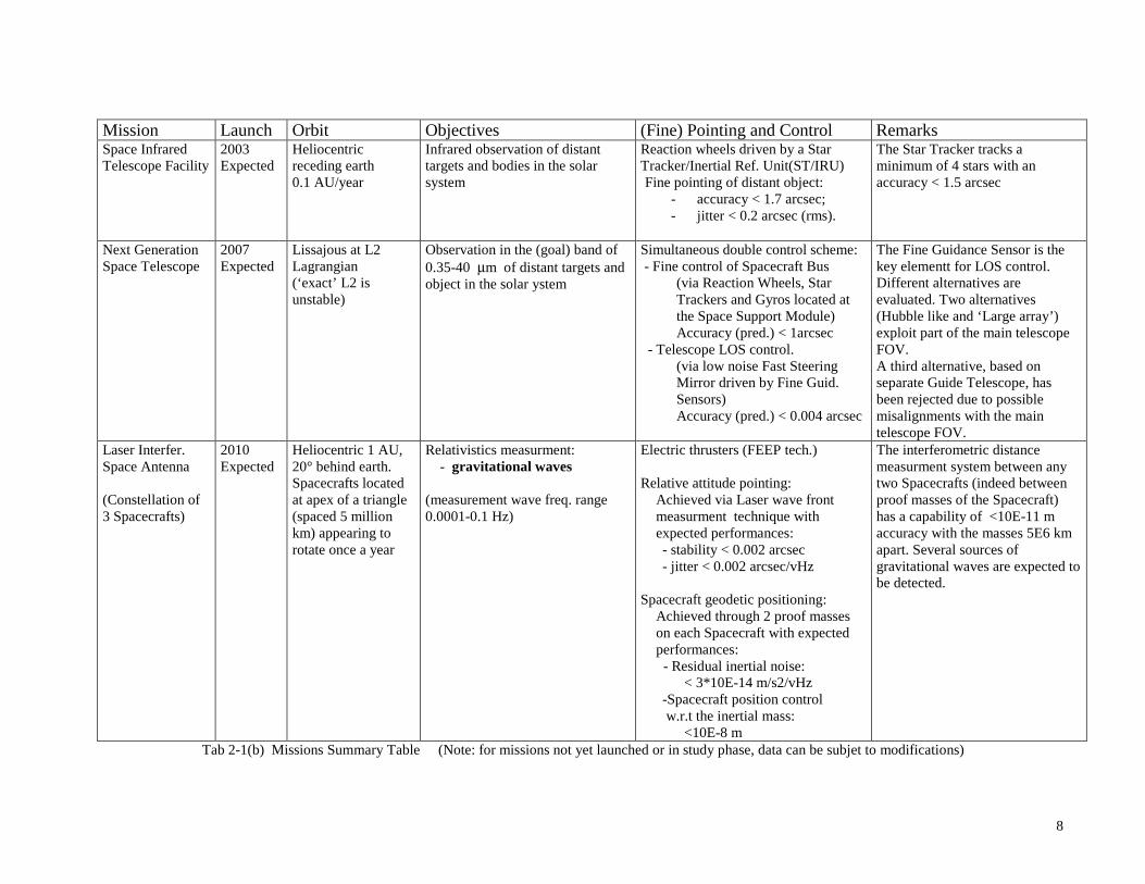
Mission Launch Orbit Objectives (Fine) Pointing and Control RemarksSpace InfraredTelescope Facility

2003Expected

Heliocentricreceding earth0.1 AU/year

Infrared observation of distanttargets and bodies in the solarsystem

Reaction wheels driven by a StarTracker/Inertial Ref. Unit(ST/IRU)Fine pointing of distant object:

- accuracy < 1.7 arcsec;- jitter < 0.2 arcsec (rms).

The Star Tracker tracks aminimum of 4 stars with anaccuracy < 1.5 arcsec

Next GenerationSpace Telescope

2007Expected

Lissajous at L2Lagrangian(‘exact’ L2 isunstable)

Observation in the (goal) band of0.35-40 µm of distant targets andobject in the solar ystem

Simultaneous double control scheme: - Fine control of Spacecraft Bus

(via Reaction Wheels, StarTrackers and Gyros located atthe Space Support Module)Accuracy (pred.) < 1arcsec

- Telescope LOS control.(via low noise Fast SteeringMirror driven by Fine Guid.Sensors)Accuracy (pred.) < 0.004 arcsec

The Fine Guidance Sensor is thekey elementt for LOS control.Different alternatives areevaluated. Two alternatives(Hubble like and ‘Large array’)exploit part of the main telescopeFOV.A third alternative, based onseparate Guide Telescope, hasbeen rejected due to possiblemisalignments with the maintelescope FOV.

Laser Interfer.Space Antenna

(Constellation of3 Spacecrafts)

2010Expected

Heliocentric 1 AU,20° behind earth.Spacecrafts locatedat apex of a triangle(spaced 5 millionkm) appearing torotate once a year

Relativistics measurment: - gravitational waves

(measurement wave freq. range0.0001-0.1 Hz)

Electric thrusters (FEEP tech.)

Relative attitude pointing:Achieved via Laser wave frontmeasurment technique withexpected performances:

- stability < 0.002 arcsec - jitter < 0.002 arcsec/vHz

Spacecraft geodetic positioning:Achieved through 2 proof masseson each Spacecraft with expectedperformances: - Residual inertial noise:

< 3*10E-14 m/s2/vHz -Spacecraft position control w.r.t the inertial mass: <10E-8 m

The interferometric distancemeasurment system between anytwo Spacecrafts (indeed betweenproof masses of the Spacecraft)has a capability of <10E-11 maccuracy with the masses 5E6 kmapart. Several sources ofgravitational waves are expected tobe detected.

Tab 2-1(b) Missions Summary Table (Note: for missions not yet launched or in study phase, data can be subjet to modifications)

9

Mission Launch Orbit Objectives (Fine) Pointing and Control RemarksHyper TBD

(Study)Sun Synchronous Relativistic measurment:

- Inertial Drag (gravitim.)Physics: - Determination of fine

structure constant; - Investigate distinct sources

of matter-wavedecoherence.

Electric thrusters (FEEP tech.)High precision Star TrackerAtomic GyroscopesAtomic Accelerometers

Fine pointing to Guide Star: - accuracy <0.02 arcsec

(Position control achieved via ‘proof masses’

with residual non gravit. accel.<2*10

10−

m/s² )

Very innovative atomic gyrosand accelerometers. They arerealised using four on boardcold atom interferometers.The achievable gyroscopessensitivity is <E-12 rad/sec(about 2*10E-7 arcsec/sec)

MAXIM Pathfinder

(Constellation of 2Spacecrafts: oneOptics S/C and oneDetector S/C)

TBD(Study)

Far from LEOorbit (either driftaway or deepspace).The two S/Cs arelocated 450 kmapart.

Mapping of X-ray sources witha resolution of 0.0001’’

Precision thrusters

Optics S/C attitude pointing:Achieved via two visible lightinterferometers viewing stars approx.perpendicular to the X-ray LOS and to eachother. Expected perf.:

- P/Y stabil. < 0.0003 arcsec - R stability < 20 arcsec

Detector S/C positioning and attitude pointing:Positioning is achieved via Laser retroreflectors data (Laser Ranging Systemlocated on Optics S/C). Expected perf.:- Lateral stability < 5 mm- Focal stability <10 meters

- P/Y/R stabil. < 20 arcsec

The Optics S/C P/Yknowledge is expected in theorder of 0.00005 arcsec.The Detector S/C LateralKnowledge is expected in theorder of 50µm.

Darwin(Constellation ofseven S/Cs: sixcollectors and onecombiner)

TBD(Study)

One LagrangianPoint. Optical baseline 100-200 m.

Detect Earth-like planets byperforming observations in theI/R range (5-20µm).

Electric thrusters (FEEP tech.)

-Pointing per axis: 0.01-0.02 arcsec

Optical path difference keptbetter than 5 nm.

Tab 2-1(c) Missions Summary Table (Note: for missions not yet launched or in study phase, data can be subjet to modifications)

10

3. REFERENCE IN ORBIT SCENARIO FOR SPACECRAFTS RELATIVE CONTROLEVALUATION

This paragraph summarizes the main characteristics of the In Orbit Scenario proposed as reference for specificevaluations on the relative control aspects issues. The following area are adressed:

• proposed reference in orbit experiment mission;• relative control acquisition and keeping and reference requirements.

The proposed mission is based on the outcomes of “ Conceptual Investigation of a Relativistic In OrbitExperiment Mission Requiring Very Demanding S/Cs Relative Control “ performed in the frame of the 2nd yearSeminars of the Doctorate School and covered in detail in ref. [55] and ref. [56] with a summary reported inAnnex 2.

3.1 Proposed In Orbit Experiment Mission

The mission considered is aiming at some indications in support to the presumed unified nature of thegravitation and electromagnetic fields.The unified theories revised for this purpose have been the ones based on a four dimensional continuum space-time non-Riemannian and in general endowed by a non symmetric fundamental tensor gαβ and a non-

symmetric connection Γ βγα . The key investigated aspect was how to reveal a possible non symmetry of the

fundamental tensor, and of the connection coefficients, in relation to the presence of electro/magnetic fields.The topic of field unification is extremely challanging and no consensus has been so far reached within thescientific community on the interpretation of the Unified Field Equations proposed by Einstein and others bothin the basic formulation and in the possible variants with sources. However the impressive and progressiveachievements in space technology may allow to conceive future space operational scenarii which may supportsome possible verifications on such a challanging subject.

A possible experimental approach which could provide some indications on the subject of non-simmetry ofspace-time is the investigation of the equation of motion for photons travelling in a unified non symmetric background metric and could be based on the following steps:

a highly collimated laser light beam (photons) is fired toward a very distant target sensor arraywhere the ‘spot’ can be centroided;

in the initial part of the laser beam trajectory, extremely high electric/magnetic fields (withappropriate geometrical orientations) are applied in confined regions;

upon the application of such fields the spacetime metric can be fleebely distorted rendering thefundamental tensor slightly non symmeteric;

the effect of such non symmetries could be a swing in the beam direction (although very small)that can be revealed as a very small change of the ‘spot’ centroid at the distant target.

The experiment could then be implemented by means of three coorbiting Spacecrafts, which can be named theGun the Distorter and the Target, placed in geostationary orbit as schematically shown in fig. 3.1-1.The Gun is an extremely accurate pointing platform and is equipped by a focussable laser source. The laserbeam is pointed toward the Target Detector Array forming a “spot” on it.At the initial part of its trajectory the laser beam crosses a volume, placed at the Distorter and possiblyprotruding from it, where very high electric-magnetic fields can be generated. These fields (when activated)could impart the beam a very small swing that could be detected at the Target Detector Array as a minute laserspot transversal displacement.The motion has been studied for different specific cases inside a ‘distorsion area’ where properly orientedelectric/magnetic fields are generated. In all the evaluated cases (see [55] and [56] and summary in Annex 2) a

11

Gun S/C

Distorter S/C

Target S/C

Laser Beam

GEO Orbit

Thousands of kilometers Tens of meters

Detector array

Laser Beam (distorted)

Fig. 3.1-1 Proposed in orbit experiment mission

non null swing appears and the photon motion seems affected, according to the different assumptions taken(geometrical entities which play the role of the electromagnetic tensors, structure of equation of motion, ….),by the presence of the fields.

Reference Experiment Mission

Taking into account the discussed results, an experimental scheme can be considered according to thefollowing schematics (fig. 3.1-2) :

Sensor target

Swing

Metric distorter

Laser source

L

L sep

(Electromagnetic fields F)

Laser spot (prturbed)

Laser spot (unperturbed)

Z

Y M

Fig. 3.1-2 Experiment schematics

where the objective would be to detect (at the target sensor) the transversal displacement M of a laser beam.Such a displacement would be a magnification, through the long distance Lsep, of the fleeble angular swingexperienced by the beam while crossing the ‘metric distorter’. Inside it the following types of terms contributeto the swing (see also references):

2

space

FFA

∂∂⋅⋅ or FD

space

mwith

space

mm ⋅−=⋅

2

2

∂∂

∂∂

where F is the generated field and where the coupling constants A, D, …. are unknown. In the variouscombinations these terms control the second derivative of the transversal displacement.

As pointed out the expected quantitative amount of such a displacement depends also on the numerical valueof coupling costant(s) which are not known. The determination of such constant(s) would then be part of the

12

experiment itself. It therefore turns out that the transversal beam displacement at the target (see fig. 3.1-2) isobservable if the coupling constant(s) allow for an actual displacement which exceed the resolution on themeasurment M.For example considering the second case reported in Annex 2, the equation for the displacement M can be putin the form:

⋅⋅=

==

=∂∂

==

⋅⋅

∂∂⋅≅

mkg

sCoulombconstant coupling ddimensioneUnknown B

(m) S/CTarget theand S/C Pointing hebetween t distance SeparationL

(m)lenght distorter EquivalentL

)(Volt/m z coordinate beamlaser at thegradient Fieldz/F

(Volt/m) z coordinate beamlaser at the FieldF

(m) target at thent DisplacemeM

LLz

FFBM

2

sep

2z

z

sepz

z2

and the displacement will then be observable if:

=

⋅⋅

∂∂

>

(m) M measurment on thesolution ReMres

LLz

FF

MresB

sepz

z

In case of fields and geometries in the following range:

==

=∂∂=

(m) 10Lsep

(m) 10L

)Volt/m(10zF/

(Volt/m) 10F

7

27

7

the observability condition would becomes (see also plot in fig. 3.1-3): 1110

MresB >

No guess can presently be done on the actual value of the coupling constant(s) axcept that it will likely be verysmall.

0.01

B(Q*s²)/(kg*m)

Mres (µm)0.1 1 10 100 1000

1510−

1410−

130−

Observability Area

Non Observability Area

Fig 3.1-3 Observability condition for the displacement (example only)

13

3.2 Relative control acquisition and keeping and reference requirements.

From a nominal point of view the control of the three S/Cs ought to be performed with the following scheme:- constant GEO position keeping with respect an earth fixed frame and therefore constant S/Cs

relative separation;- constant attitude keeping with respect an earth fixed frame and therefore constant S/Cs relative

attitude.

Indeed even starting from initial contitions of zero errors and zero errors speed (both for position and attitude),anyhow basically impossible, the following actual conditions are encountered:

- the position (absolute and relative) tend to be modified by the force disturbance effects of solarradiation pressure, solar-lunar attractions and earth tesseral effects;

- the attitude (absolute and relative) tend to be modified by the torques induced by the solar radiationpressure and the gravity gradient torque (even if these last effects would be negligible in GEO formoderate size and well balanced S/Cs).

In order to compensate for the disturbances, trying to achieve above stated nominal control scheme, appropriatecontrol actions can be applied with the objective of:

- guarantee the short term relative control in order to be able to perform the scientificexperimentation.

- guarantee the long term overall S/Cs orbital configuration.

During compensations other disturbances will in turn be injected in the system and are related to:- sensors errors;- actuator (thrusters) errors;- control action algorithm limited performances.

Given the nature of the scientific investigation to be performed, the operational approach considered can bebased on the following points:

1. the Pointing S/C need be optically aligned onto the sensor surface array of the Target S/C forsequences of Basic Time Interval (BTI) each allowing the execution of a portion of scientificinvestigation. During each BTI the vibration on the Pointing S/C and Target S/C need be reallyminimum in order not to disturb the scientific measurment;

2. we can take the BTI to a reference value of some tens of seconds and during this time the onlypractical source of disturbances (with frequency content) are the ones related to the fluctuations ofthe solar radiation pressure;

3. during BTI the Pointing S/C Line of Sight tend to drift away from the target (due to the effects ofnon zero initial relative angular speed rate and the disturbance torques due to the radiation pressureand gravity gradient). Furthermore the Pointing S/C position (as well as the Target S/C position)tend to drift due to non zero initial speed rate, radiation pressure, sun/moon perturbations, earthpotential distorsion terms;

4. after each generic BTI the actuators can be fired within a suitable Firing Time (FT) in order to:- for the Pointing S/C generate the appropriate starting conditions to properly initiate and

allow the development of the next BTI by re-centering the Pointing S/C Line of Sight to theTarget S/C;

- for the Target S/C recover the drifting attitude ( only within a coarse accuracy).5. the allowed FT for the actuators can be taken to a reference value of few hundereds of seconds;6. the S/Cs position recovery can be performed every time the position error exceed a maximum

allowed value. The recovery need be performed by thrusters in the class 20 (mN) and in timeperiod not overlapped to the attitude control.

14

Concerning more specifically the scientific investigation it can be implemented by:- perform an initial target acquisition;- repeat for a sufficiently large number of times the combined sequence:

BTI followed by a FT.Above combination could be repeted for e.g. tens of times (as shown in the schematics of fig. 3.2-1).

PositioningManoeuver(Motor Firing)

InitialPosition Motor

Firing

Free Drift

Target sensorArray

Initial Positioning Manoeuver→Free Drift→Fire→Free Drift→Fire→ Free Drift→Fire→

Fig. 3.2-1 Relative pointing control strategy (not to scale)

During the Basic Time Interval (BTI) the real part of the scientific investigation is performed. Although thescientific aspects will not be furthermore addressed, the following considerations are worth being pointed out:

every 0.5 second or a fraction of this (indicative) three types of measurments are performed by usingthe target sensor array signals:1) background illumination (the laser beam is blocked to reach the target sensor array);2) laser illumination pattern with the electric/magnetic fields activated;3) laser illumination pattern with the electric/magnetic fields not activated or modulated.

in real time the following computations can then be carried out:centroiding computation of signal 2 minus signal 1 above;centroiding computation of signal 3 minus signal 1 above;

15

the comparison of the centroids trajectories (reconstructed in the free drift passage) could provide anindication of the searched ‘laser beam transversal displacement’.

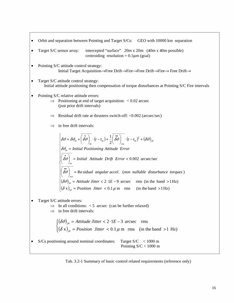
Concerning the control requirements to be utilised, for the detailed evaluations, the couple formed by thePointing S/C and Target S/C will be considered. The requirements are summarised in tab. 3.2-1 and areherebelow briefly discussed.

Distance between Pointing and Target S/Cs.GEO orbit is characterised (with respect to LEO orbit) by:

- large allowed S/Cs separation;- no atmospheric drag and no atmospheric related optical disturbances;- reduced disturbances of earth potential terms and reduced gravity gradient related torques.

The separation between the S/Cs ought to exploit the advantages allowed by GEO orbit and can be taken 10000km as reference. It can be reduced to some hundereds kilometer or further increased (see sketch in fig 3.2-2showing the spacecrafts at different separations).

Pointig S/C control strategy (and Target S/C control strategy)(See fig. 3.2-1 and previous relevant discussion)

Target S/C sensor array.The dimensions of the Target S/C sensor array ought to be compatible with the foreseen technologicalpossibilities (for manufacturing, launch, in orbit deployment). A reference “surface” of approximately20m x 20m is well in line with present standard technology and can be taken as reference for therelative control evaluations (also larger surfaces of 40m x 40m could be considered).The centroiding measurment resolution (which should be taken as low as possible) is related to thebasic transducer technology employed for the array.A resolution requirement of 0.1 µm is considered.

Pointing S/C relative attitude error (Pointing S/C relative to Target S/C).Based on the described control strategy, the target acquisition should be performed with a relativeaccuracy better than +/-0.02 (arcsec). This would allow a good sensor surface exploitation since wouldcorrespond to approximately 10% of a 20 (m) size sensor (center to boarder distance).The attitude drift rate (between subsequent target acquisitions) shall support the illumination of theTarget sensor array for an acceptable time. A drift rate < 0.002 arcsec/s at the beginning of each freedrift interval allows (if it were the only source of drift) a permanence in the order of 100 s.The attitude jitter (see schematics in fig. 3.2-3) can be a very difficult requirement to be met since itshall be such not to cause beam ‘spot’ oscillations at the Target sensor array larger than e.g. 0.1 µm (theassumed sensor resolution) in a frequency band which may potentially imply signal aliasin effects.Given the involved geometries the attitude oscillations can be required to be < 2·1E-9 arcsec rms (inthe band > 1 Hz).The position jitter translates directly in beam ‘spot’ jitter and can be required < 0.1 µm rms (in the band>1 Hz).

Target S/C attitude error.No major requirements are placed on the maximum attitude error for the Target S/C. The limitingfactor is not related to control aspects but to the power of the ‘illuminating laser’ onboard the TargetS/C. A reference of 5 arcsec (but it could even be larger) is considered for reference; this would allowto keep the divergence of the beam to 10-20 arcsec enough to guarantee sufficient power to reach thehigh accuracy interferometer onboard the Pointing S/C.

16

• Orbit and separation between Pointing and Target S/Cs: GEO with 10000 km separation

• Target S/C sensor array: intercepted “surface” 20m x 20m (40m x 40m possible)centroiding resolution = 0.1µm (goal)

• Pointing S/C attitude control strategy:Initial Target Acquisition→Free Drift→Fire→Free Drift→Fire→ Free Drift→

• Target S/C attitude control strategy: Initial attitude positioning then compensation of torque disturbances at Pointing S/C Fire intervals

• Pointing S/C relative attitude errors: Positioning at end of target acquisition: < 0.02 arcsec

(just prior drift intervals)

Residual drift rate at thrusters switch-off: <0.002 (arcsec/sec)

in free drift intervals:

( ) ( ) ( )

( )( )

><=

>−⋅<=

=

<=

=

+−⋅

+−⋅

+=

••

•

•••

Hz) 1 band (in the rms m 1.0 x

Hz) 1 band (in the rms arcsec 912

) ( . Re

arcsec/sec 002.0

2

1 2

µδδϑ

δϑ

δϑ

δϑ

δϑδϑδϑδϑδϑ

JitterPosition

EJitterAttitude

torquesedisturbancnullable non celangular acsidual

ErrorDriftAttitudeInitial

ErrorAttitudegPositioninInitial

tttt

jit

jit

res

in

in

jitinres

inin

in

• Target S/C attitude errors: In all conditions: < 5 arcsec (can be further relaxed) in free drift intervals:

( )( )

><=

−⋅<=

Hz) 1 band (in the rms m 1.0 x

rms arcsec 312

µδδϑ

JitterPosition

EJitterAttitude

jit

jit

• S/Cs positioning around nominal coordinates: Target S/C < 1000 m Pointing S/C < 1000 m

Tab. 3.2-1 Summary of basic control related requirements (reference only)

17

Concerning the jitter, at least along one direction (see schematic of fig. 3.2-4), it shall be such not toinduce sensor dispacements larger than the resolution. A requirement < 2·1E-3 arcsec rms (in the band> 0.1 Hz) is considered for reference. The position jitter translation is required < 0.1 µm rms (in theband > 1 Hz) as for the Pointing S/C.

Target 2

Target 1

Distorter 1

Distorter 2

Gun

Athmosphere

EARTH

~6400 km ~42.000 km

d 2

d 1

Case of GEO orbit (not to scale)

Target 2

Target 1

Distorter 1

Distorter 2

Athmosphere

EARTH

~6400 km

~6900 km

d 2 d

1

Case of LEO orbit (not to scale)

Gun

d1 = 1000 km d2 = 10000 km

d1 = 1000 km d2 = 3000 km

200 - 300 km

Fig 3.2-2 Sketch of S/Cs placed on GEO orbit (Vs. LEO orbit)

18

S/Cs positioning around nominal coordinates.The positioning control does not result in a stringent requirement. It can be set to +/-1000 (m) for boththe Target and the Pointing S/Cs. This allows the Target S/C to be within the Field of View of theRelative Attitude Sensor placed at the Pointing S/C even with no S/W compensation for the positionoffsets.

Laser

d teta

Target sensor array

10000 km separation

Beam displacement at target due to Pointing S/C jitter

Pointing S/C

Fig 3.2-3 Pointing S/C jitter effects schematics (not to scale)

C.M

V bar

Laser Beam

Beam 'Spot'

Theta

Oscillations (jitter) on Theta causes transversal sensor array oscillations

Target sensor array

Fig 3.2-4 Target S/C jitter effects schematics

19

4. SENSORS

During the scientific mission phase it is necessary to perform the optical alignment of the Pointing S/C to theTarget S/C in a very accurate way although no major requirements are placed on position control.The sensors utilized shall be able to guide the Line of Sight alignment independently on the S/Cs position (e.g.with respect to a nominal alignment frame) and independently on the accuracy of position knowlwdge.The sensors here evaluated to support the control problem, are of three types: arcsec class absolute attitudesensors, ultra precise relative attitude measurment systems and advanced solid state gyroscopes. The relativeattitude measurment system is of extreme importance. It has been decided to evaluate a sensor which is basedon flat reflectors and does not make use of curved optics (like in the relativistic mission Gravity Probe B andLISA). This because flat reflectors can be manufactured with extreme flatness thus allowing higherpotentialities in perspective.The sensor work on the principle of wave front splitting interferometry and does not need any positioninformation on the Spacecrafts. It has been evaluated in detail in the frame of the 2nd year Seminars of theDoctorate school [35] and a summary is reported in Annex 3.The positioning sensors (for orbital location) has been assumed with performances in line with the capabilitiesof present techniques for satellite position determination (e.g. Laser Ranging, GPS ‘side lobe’ utilisation atGEO and RF based techniques) but no ultra precise measurements with respect to ‘geodetic proof masses’ arenecessary.

4.1 Absolute attitude sensors

The capability to perform precise absolute attitude determination to the arcsec level can be tackeld by means ofStar Tracker sensors capable to harmonise two contrasting requirements:

- absolute attitude determination capability to a medium accuracy level (e.g. 10 arcsec level range);- improvement of the absolute attitude determination to the arcsec level range (typical of

astronomical instruments).

As a basic approach the combination of two Star Trackers can be used:- one Autonomous Star Tracker with ‘lost in space’ capabilities and a moderate Field of View;- one very high accuracy Star Tracker with (Very) Narrow Field of View.

The first type Star Trackers can provide the absolute attitude of the Spacecraft with respect to the CelestialReference Frame in terms of quaternions starting from whatsoever S/C condition with no need of other sensorsor information. These sensors are basically available ‘off the shelf’ in the space commercial market.The second type of Star Trackers are very special products and depending on the design/customisationapproach may be devised to provide the angular position of the tracked star/s with respect to the OpticalBoresight of the instrument or, if supported by a specific Star Catalogue and processing, the absolute attitude ofthe Spacecraft with respect to the Celestial Reference Frame. These sensors are typical for application drivingastronomical instruments and can provide full performances at a much lower Spacecraft attitude rate than thefirst type. If used for absolute attitude determination they likely need be initialised (with initial attitudeconditions) to an accuracy in the range of sone tenths of degrees which can be provided either by theAutonomous Star Tracker or even by Sun/Earth sensors. Very few manufactures can provide reliable sensors ofthis second type.Some basic features of star trackers will be presented and candidate high performance units identified in orderto derive a reference set of characteristics which can be used as inputs to a simulation activity (see ref.[21],[22], [23], [24], [25], [26]).

The operating principles will only be briefly reviewed (since the star trackers works according to a classicalapproach) with the main scope to allow a better understanding and interpretation of the given performances.

20

Operating principle

The core sensing part of the Star Tracker is composed by the optics and the sensor array, typically a CCD, asschematised in fig. 4.1.-1. The image of the stars in the field of view form on the CCD and, based on theseinformation, the orientation of the Star Tracker reference Frame (STF) can be computed with respect to theCelestial Reference Frame (CRF).The foollowing steps are noted:

- the images of the stars are formed on the CCD sligtly defocused in order to illuminate more thanone pixel each star;

- the images formation is allowed to occure for a proper observation time (e.g.0.05 sec-0.5 sec) priorthe CCD being red;

- on the most bright star images (e.g. up to 6) a centroiding operation is then performed in order tocompute the ‘central position of each star image’;

- the defocussing allows the determination of the star position (on the CCD) with aresolution in the range of 1/5 to 1/20 of the pixel dimensions depending on the techniqueused (if no defocusing were done then a maximum of one pixel size in resolution would beachieved);

- the pattern of the observed stars (basically their relative geometrival layout) is compared in an onboard Star Catalogue to determine which stars are actually being obseved;

- the star pattern position on the CCD allow to determine the orientation of the STF with respect tothe pattern itself;

- being known the stars, the orientation of the STF with respect to the absolute frame used in theCatalogue (e.g. the CRF) can therefore be computed.

The performances achievable by the Star Tracker depends on specific factors like:- the number of stars being observed;- the brightness of the observed stars;- the Field of View and CCD dimension (pixel number);- the observation time (integration time on the CCD).

and a balanced selection of them is necessary.The final performances will result in a blend and compromise among many factors including also the specifictechnological ones:

- mechanical and optical tolerancing and alignment;- alignment sensitivity to temperature variations;- degradation of parts with operating time in space conditions;- detailed electronic design;- algorithms utilisation and calibration;

which should indeed be in hand and under control of the equipment manufacturer.

Mathematical ModelThe modern Autonomous Star Trackers provide in output the orientation of the SRF with respect to anabsolute frame (like the CRF) via quaternions.The matematical model can be described by the following equation:

tm qIq ⋅+= ]2

1[ ε

where:=tq True quaternion of the frame SRF with respect to the frame CRF (4x1)

21

=mq Measured (by Star Tracker) quaternion of the frame SRF with respect to the frame CRF (4x1)

I = Identity Matrix (4x4)

MatrixError

zyx

zxy

yxz

xyz

0

0

0

0

=

−−−−

−−

=

δδδδδδδδδδδδ

ε

=zyx δδδ ,, Axis components errors

Above model hold for low values of axis component errors (which is the case considered). The structure ofeach axis component error encompasses the following contributions:

nxolfxbxx δδδδ ++==bxδ constant residual bias=olfδ orbital and low frequency bias

=nxδ measurement noise

The constant residual bias can be modeled as an unknown constant and is the bias gathering mechanical, opticaland sensor residual misalignments.The orbital and low frequency bias can be modeled as harmonics with unknown amplitudes and phases andgather the thermal effects along the orbit and the errors associated to the star identification and catalogue. Themeasurement noise can be modeled as a white sequence (in the discrete domain).

For Star Trackers devised to provide the angular position of the tracked star/s with respect to the OpticalBoresight of the instrument (rather than quaternion) the model reduce to three errors ,,, zyx δδδ abovedescribed. It will be part of the complete attitude measurment system to process such errors in a more generalspacecraft attitude model.

Z (boresight)

X

Y

Optical lens

Star 1Star 2

Star 3

CCD array

f (approx)

Fig. 4.1-1 Simple illustration of the Star Tracker core sensing part (three stars shown)

22

4.1.1 Autonomous Star Trackers (‘Lost in Space’ type)

In this section the basic features of three Autonomous Star Trackers are reported. To allow this, the specificproducts of three of the most well known manufacturers of Star Trackers in the world are presented andsummarised in Tab. 4.1.1-1. All such products have Medium Field of View features and ‘lost in space’capabilities in the sense that they can provide full Spacecraft attitude information from whichever initialconditions with no need of other information.The data have been taken from the catalogues for these equipments. Sometimes the declared data refer to nonhomogeneous conditions and, in order to put them in a comprehensive summary table, some adjustment havebeen done when the data were referred to different conditions (e.g. σ value). Some notes have also been added.The three products are of high performance profile and, apart some differences, can be considered to belong toa similar functional class. For our purposes we refer to the performances of the A-STR Autonomous StarTracker from Galileo Avionica (see picture in fig. 4.1.1-1) as a reference equipment.

4.1.2 Narrow Field of View Star Tracker

In order to improve the performances on absolute attitude determination (complementing the ones achievableby means of the fully autonomous star trackers previously described), the possibility to utilise a Narrow Fieldof View star tracker instrument has been investigated.In this respect specific contacts have been undertaken with the manufacturer company Galileo Avionica(Florence).

A very accurate instrument is available from this company and its core configuration is composed by an OpticalHead (OH) and an Electronic Unit (EU). This instrument (indeed a Narrow Field of View star tracker) is undercontinuous enhancements and the present version, depicted in fig. 4.1.2-1, has the impressive performances asreported in tab. 4.1.2-1. In the core configuration the star tracker provides the position (and magnitude) of theobserved stars with respect to the SRF and, in the enhanced version, by using embedded star catalogues, patternrecognition and attitude determination algorithms, is able to autonomously provide attitude information in theform of quaternions; for this operation mode, due to the narrowness of the Field of View, an initial attitudeinformation need be provided by some external sensors. Alternatively the core star tracker configuration can beused coupled to an autonomous star tracker.The overall performances achievable render suitable the utilisation of this instrument also for thepointing of astronomical instrument and in general attitude determination in situations with lowattitude rate changes (in the specific case < 180 arcsec/sec).For our purposes we consider the HRA-STR High Resolution Star Tracker as a reference equipment.

Fig. 4.1.1-1 Picture of the A-STR (AutonomousStar Tracker) – Galileo Avionica

Fig. 4.1.2-1 Picture of the HR-STR (High ResolutionStar Tracker) – Galileo Avionica

23

Feature CT-633Ball Aerospace

A-STRGalileo Avionica

SED 16Sodern

Field of View (degrees) 20°x20° 16.4°x16.4° 25°x25°

CCD size (pixels) 512x510 512x512 (not given in basic catalogue)

Attitude Determ. Perf. (1σ) (arcsec)- bias- orbital & low frequency- random noise

Pitch/Yaw Roll (boresight)

10 (incl. bias) 40 (incl. bias)6 (@ 0.2°/s) 30 (@ 0.2 °/s)(declared per star over temp. range)

Pitch/Yaw Roll (boresight)3.3 42.4 104.3 (@ 0.5°/s) 44 (@ 0.5°/s)(derived from declared data at 3σ)

Pitch/Yaw Roll (boresight)4.6 3.34.3 101-3.3 6.8-18(derived from declared data at 3σ;noise ranges based on differentcatalogues data)

Star Sensitivity Range(Visible Magnitude)

0.1 to 4.5 1.5 to 5.5 (not given in basic catalogue)

Max Number of Trackable Stars 5 10 (not given in basic catalogue)

Max Spacecraft Attitude Rate (°/sec)(for mantain track)

(not given in basic catalogue) 10 10

Data Update Rate (Hz) 5 10 10 (max)

Attitude (initial) acquisition time (sec) < 60 sec (> 98% probab.) <15 sec (@1°/sec and >99.9% probab.)<20 sec (@2°/sec and >95% probab.)

< 60 sec (> 99.9% probab.)

Attitude Output Format Quaternion in the embedded size 2000Star Catalogue

Quaternion in the J2000 Star CatalogueRaw star dataHousekeeping data

(not given in basic catalogue)

Interfaces Data bus: 1553 or 1773 or RS 422Supply: 28+/-6 Volts

Data bus: 1553B or RS422Supply: 22-50 Volts

Data bus: 1553 or RS422Supply: 16-55 Volts

Dimensions 135 (D)x 142 (L) (without baffle) 160(H)x146(W)x158(W) (without baffle)250(L)x190 (D) (standard baffle)

170x144x147 (without baffle)278x158x147 (including baffle)

Mass (kg) 2.5 (without baffle) 2.5 (without baffle)0.4 (standard baffle)

2.9 (including baffle)

Power consumption (W) 8 (@ 20°C) 10.5 (@20°C including 1553 I/F) 8

Tab 4.1.1-1 Autonomus Star Tracker Expected Performances (data derived from catalogues)

24

Feature HR-STRGalileo Avionica

Field of View (degrees) 4°x 4°

CCD size (pixels) 512 x 512 (17µm x 17µm / pixel)

Accuracy (2σ) (arcsec)• Stars position

- bias and low frequency (central FoV) (total FoV)

- random noise

• Attitude (multistar) in Autonomous Configuration (N = 3 as worst case)

- bias and low frequency

- random noise

(Accuracies referred to CCD MeasurmentReference Frame)

X,Y

0.351.35

1.3

Pitch/Yaw Roll (Boresight)

0.8 27

0.7 25

Star Sensitivity Range(Visible Magnitude)

Up to 8.3

Max Number of Trackable Stars 10

Max Spacecraft Attitude Rate (°/sec)(for mantain track)

0.05 (or 180 arcsec/sec)

Data Update Rate (Hz) 2

Attitude Output Format Positions of detected stars with respect to the SRF;Quaternions (in Autonomous Configuration)

Interfaces Data bus: MIL 1553BSupply: 20 – 50 Volts

Dimensions (mm) OH: 120x219x140 (without baffle) EU: 220x200x65

Mass (kg) OH: 3.2 (without baffle) EU: 1.8

Power consumption (W) <11 @ 20°C<14 @ 60°C

Tab 4.1.2-1 High Resolution Star Tracker (with Narrow Field of View)-Galileo AvionicaPerformances of the Core Platform

25

4.2 Interferometric Relative Attitude Sensor

The high accuracy relative attitude sensor considered is based on laser wavefront splitting interferometry whoseoperating principle and mechanisation is described in detail in RD[35].The proposed sensor exploits a suitable number of reflectors to create an interference pattern whose positionon a detector plane is a function of the S/Cs relative pitch and yaw angles.

The two key elements determining the performances in terms of pitch and yaw information are theinterferometer located on the Pointing Spacecraft and the quality of the laser beam casted by the TargetSpacecraft as schematically shown in fig. 4.2-1.

Target S/C

IlluminatingLaser beam

Pointing S/C(Interferometer)

Beam Wavefron(Coherence)

α (Pitch)

Pointing Direction

Wavefront Intakes

Fig. 4.2-1 Application Scheme of the considered relative attitude sensor (wavefront splitting interferometry).(Two dimensional drawing: only pitch angle shown)

Concerning the interferometer the approach based on the utilisation of flat reflectors is considered. Suchreflectors are the easiest to manufacture (at very high optical quality) and to align and can be arranged so as tocreate an opportune interferometric pattern.As far as the laser beam it has be appropriate quality, ideally:

- frequency placed at a good level of the detector quantum efficiency curve;- single transversal mode TEM00 ;- single cavity longitudinal mode (or at least a multimode with an overall frequency banwidth range

to present an acceptable coherence length);- sufficient optical power to allow a good processing of the fringe signal levels.

4.2.1 Relative attitude sensor configuration

The interferometric sensor configuration finally considered for the studied scenario is based on three secondaryreflections as shown in fig. 4.2.1-1 and the main characteristics are herebelow summarized:

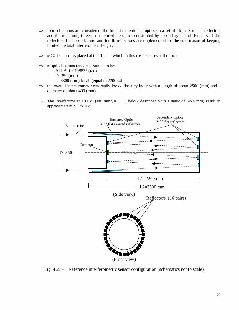
26

four reflections are considered, the first at the entrance optics on a set of 16 pairs of flat reflectorsand the remaining three on intermediate optics constituted by secondary sets of 16 pairs of flatreflectors; the second, third and fourth reflections are implemented for the sole reason of keepinglimited the total interferometer lenght;

the CCD sensor is placed at the ‘focus’ which in this case occures at the front;

the optical parameters are assumed to be:ALFA=0.0198837 (rad)D=350 (mm)L=8800 (mm) focal (equal to 2200x4)

the overall interferometer externally looks like a cylinder with a length of about 2500 (mm) and adiameter of about 400 (mm);

The interferometer F.O.V. (assuming a CCD below described with a mask of 4x4 mm) result inapproximately 93’’x 93’’

Entrance Optic# 32 flat skewed reflectors

Detector

Secondary Optics# 32 flat reflectors

Entrance Beam

D=350

L1=2200 mm

L2=2500 mm

(Side view)

(Front view)

Fig. 4.2.1-1 Reference interferometric sensor configuration (schematics not to scale)

Reflectors (16 pairs)

27

The entrance ‘mirrors’ can be made simply by substrate optical material surfaces (e.g. ULE with n=1.4828 @0.589 µm) very flat and polished which sees the incoming beam at a very high incidence angle ( in this caseabout 89.43°) while the secondary optics which sees the beam at a very low incidence angle (in this case about1.139°) can be constituded by actual mirrors. The dimensions for the two types of mirrors are assumes as:

- entrance reflectors: 7 (mm)x 350(mm);- secondary mirror: 8 (mm)x 8 (mm);- Rt ≈ 0.9 (cumulative of all reflections)

Mismatch < 0.02

Herebelow are reported the main features of CCD detector and illuminating laser source that can be consideredfor an initial performances evaluation.The CCD considerd (Philips FT18 shown in fig 4.2.1-2) is operating in the visible range, in line with the lasersource and is characterized by a very low pixel size, compared to similar high quality products, allowing forlimited interferometer length; the main features are the following:

- optical size: 7.68 (mm)x 7.68 (mm);- pixels number: 1024x1024;- pixel dimension: 7.5µm x 7.5µm;- conversion factor: 10 µV/el;- full well capacity: 45 kel/px (max voltage about 0.45V);- read out noise: 30 el @ 30 Hz frame rate (estimated < 25 el @ 2Hz frame rate);- shot noise: 10 el/px;- dark current: 1400 el/sec/px @ 45°C conditions;- dark signal non uniformity (after compensation): 140 el/sec/px (estimated as 10% of dark current)

@ 45°C conditions;- dark signal non uniformity (after compensation): 10 el/sec/px estimated @ +5°C (moderate

thermal conditioning);- pixel FOV: 0.1757’’.

This CCD is not space graded and the possibility to utilise it would require a specific qualification processespecially in the areas of :

- thermal vacuum;- radiation tolerancing.

The same would apply to the other commercial CCD with similar small pixels dimension available on themarket. Specific mounting solution ought to be evaluated for its installation on the interferometer.

CCD presently suitable for space have pixels dimensions of 13µm x 13µm or larger. They are of very goodperformances but would imply interferometer lenght greater than the one shown (e.g. 2.5 m instead of 1.75 m).The technology trend is however to utilize in space CCDs with pixel size progressively smaller and, formissions like the ones considered it is likely that in few years CCD of the class here considered would beavailable.As far as the laser source and optics placed on the target illuminating spacecraft, it has not been found aselection of products already available for space. For this analysis we can refer to data of good commercialproducts which could in principle be subject to an appropriate improvement and qualification process. Thecommercial products considered are derived from Melles Griot (see also fig. 4.2.1-3):

- laser type: Melles Griot CW HeNe (05LHP927);- λ= 632.8 nm;- output power> 35 mW;- transversal mode: TEM00;- coherence lenght> 1 m (typical);- polarization: linear >500:1

28

- beam divergence (prior to beam expander) ≅ 0.66 mrad = 136 arcsec- precision beam expander type: Melles Griot 09 LBM 017 (20x)- beam divergence (at the exit of the precision beam expander) ≅ 7.5 arcsec

- illumination area at 10000 km distance: disk of 363 m diameter (1/ 2e )- irradiance at 10000 km distance within 4 arcsec > 0.00000116 (W/m2)- control requirement on illuminating (target) S/C ≅ ± 2 arcsec

In case no space products would be available, the possible improvement and qualification process to beconsidered for the commercial laser and optics should cover as a minimum the following aspects:

- utilisation of al structural and casing materials with very low thermal expansion coefficients (e.g.super invar, quartz silica, zerodur);

- thermal verification/redesign for space vacuum using only conduction (and heath pipes ifnecessary);

- verification of laser thermal stability;- machining of optics with superior flatness features (e.g. > λ/20);

Four cases have been evaluated to assess the performances and summarized in tab. 4.2.1-1:

First case (‘very large’ attitude value)Total angle inclination (input) = 8.01’’Direction ψ of inclination (input) = 225° this means:

True Pitch= -5.663925’’ True Yaw=-5.663925’’

Second case (‘large’ attitude value)Total angle inclination (input) = 1.0656’’Direction ψ of inclination (input) = 13° this means:

True Pitch= 0.2397078’’ True Yaw=1.0382887’’

Third case (‘small’ attitude value)Total angle inclination (input) = 0.0102’’Direction ψ of inclination (input) = 119° this means:

True Pitch=0.0089211’’ True Yaw= -0.0049450’’

Fourth case (‘zero’ attitude value)Total angle inclination (input) = 0’’Direction ψ of inclination (input) = 70° this means:

True Pitch=0’’ True Yaw=0’’

Tab. 4.2.1-1 Summary of the considered cases

For all cases the effects of pixel finite dimensions, reflection coefficients cumulative value and mismatch, shotnoise, dark signal non uniformity and read out noise were included.

The results of the simulations (interf06.m, baric6.m) are reported in fig. 4.2.1-4 and the followingconsiderations are noted:

- the pitch and yaw measurments are very good and the observed errors are in the range from 0.001to 0.0025 arcsec (rms);

- such errors are the contribution of effects related to CCD finite pixel dimensions and statisticalnoise (going to pixel level);

- given a CCD this type of error can be reduced by reducing the angle α (basically enlonging theinterferometer) and cooling further the CCD;

- alternatively, not to enlong the interferometer, utilise CCD with smaller pixel size (which iscertainly realistic for missions potentially planned by the next decade) and always keep cooled thesensor;

29

- the centroiding algorithm utilised is quite simple and not much different from the typical ones usedin star position determination. It consists in ‘x line centroiding’ and ‘y line centroiding’ on 11pixels each. The pixels voltage outputs have been treated by an exponent of 1.2 to increase thecontribution of the high signal pixels. There are margins to improve the centroiding technique.

In the next paragraphs the biasing type errors, for many respects more critical than the ones here considered,will be discussed togheter with the need of the ‘internal metrology measurment system’.

Sensor picture Quantum efficiency curve

Fig. 4.2.1-2 CCD sensor Philips FT18

HeNe Laser schematics (Melles Griot)

Fig. 4.2.1-3 Commercial HeNe laser scheme and Precision Beam Expander (Melles Griot)

30

First caseTrue Pitch (arcsec)= -5.663925True Yaw (arcsec)= -5.663925Pitch average (arcsec)= -5.6657Pitch error rms (arcsec)= 0.0019Yaw average (arcsec)= -5.6657Yaw error rms (arcsec)=0.0019(shown 111x111 pixels = 19.5’’ FOV)

Second caseNominal pitch (arcsec)= 0.2397078Nominal yow (arcsec)= 1.0382887Pitch average (arcsec)= 0.2403Pitch error rms (arcsec)= 8.7121e-004Yaw average (arcsec)= 1.0360Yaw error rms (arcsec)= 0.0024(shown 61x61 pixels = 10.7’’ FOV)

Third caseNominal pitch (arcsec)= 0.0089211Nominal yow (arcsec)= -0.0049450Pitch average (arcsec)= 0.0098Pitch error rms (arcsec)= 0.0011Yaw average (arcsec)= -0.0056Yaw error rms (arcsec)= 8.8168e-004(shown 31x31 pixels = 5.4’’ FOV)

Fourth caseNominal pitch (arcsec)= 0Nominal yow (arcsec)= 0Pitch average (arcsec)= -8.7601e-005Pitch error rms (arcsec)= 0.0013Yaw average (arcsec)= -2.0807e-005Yaw error rms (arcsec)= 0.0011(shown 31x31 pixels = 5.4’’ FOV)

Fig. 4.2.1-4 Simulation results for the three considered cases

Note: included effects of pixel finite dimensions, reflection coefficients cumulative value and mismatch, shotnoise, dark signal non uniformity, read out noise.

10 20 30 40 50 60

10

20

30

40

50

60

5 10 15 20 25 30

5

10

15

20

25

30

10 20 30

5

10

15

20

25

30

10 20 30 40 50 60 70 80 90 100 110

10

20

30

40

50

60

70

80

90

100

110

31

4.2.2 Performance degradation due to biasing effects

In this paragraph the performances of the interferometer will be discussed with respect to the degradationeffects caused by thermal and manufacturing dimensional distorsions.A substantial difference exists between the two types of effects:

- the thermal distorsions change with temperature and even assuming a reasonably narrow thermalcontrol range (however achievable by simple passive means) such distorsions fluctuate during themission;

- the manufacturing dimensional distorsions can be assumed constant and oncemeasured/compensated (e.g. in orbit) it is for all.

The attitude measurments errors induced by thermal distorsions can in principle be compensated in line (orpartially compensated) by means of a correction procedure based on temperature measurments and a thermo-mechanical model. It is however important to evaluate the order of magnitude for such errors in order toestimate the relevent impacts and the need for compensation techniques much more efficients than the onesallowed by athermomechanical model prediction.

Thermal stabilisation methods based on bath of liquid coolants (e.g. liquid He or other) will not be consideredhere for the impacts they have in operational complexity, limited operational lifetime, technical complexity andconstraints on S/C design, versatility of potential applications.

4.2.2.1 Thermal distorsion effects

In this paragraph the attitude measurment accuracy degradation caused by thermal related structural distorsionswill be discussed. For the evaluation the following assumptions are done:

- the interferometer temperature distribution is kept uniform in the range of +/ 5 °C by means ofpassive means;

- the temperature of several points of the interferometer is measured with an accuracy of +/- 0.5 °C;- a thermo mechanical model is available which allow the evaluation of the structural distorsions to a

good approximation (limited however by the temperature uncertaities measurments).

In general, given a structure, the thermal distorsions depend primarily on three factors: the type of material(indeed its CTE), the temperature variations, the geometry of parts on which the temperature variation apply.Concerning the materials, tab 4.2.2.1-1 summarises the most important ones potential candidates for spaceinterferometry structures (see also ref [36], [37], [38], [39], [40], [41], [42]).Two alternative approaches may be considered for the interferometer structure:

- laminate technologies (hybrid, reiforced) with Invar or Super Invar inserts (final overall CTE in the

order of +/- 0.1* 610− 1/°K);- assembly of structural elements obtained by machining blocks of Zerodur and/or ULE (achievable

CTE in the range of +/- 0.1* 610− to +/- 0.03* 610− 1/°K).

Let us now consider different cases of thermal inhomogeneities acting on the interferometer structure andevaluate the expected attitude drift starting from a reference initial calibrated situation of zero pitch and zeroyaw (which is anyway the final aiming control).

The evaluated cases indicates that the axial (circumferentially) non uniform gradient may constitute a seriousproblem in the operation of the interferometer if the milli arcsec (or sub milliarcsec) class performances.

32

Indeed even assuming the utilisation of a longitudinal interferometer structure with an CTE of the ULE class (0.03*E-6) and assuming to know the temperature distribution up to +/- 0.5°C, an uncompensated attitude driftin the order of some 0.01’’ can be present.A compensation technique more efficient than the one based on temperature measurment andthermomechanical model ought to be considered to detect the relative displacement (mainly rotation) of thesecondary reflective surface with respect to the primary mirrors and detector. Such rotation, once measured,can be utilised in the compensation process to eliminate (or reduce) the effects of thermal drift.The compensation technique can be implemented by means of an Internal Metrology System and issummarised at paragraph 4.2.2.3.

Material CTE range ( x 610− ) Remarks

Reinforced Fibres (Carbon/Boron +Epoxy/Cynate)

+2/-2 Good forming and shaping.Possibility to place inserts. Excellentstructural element.

Invar 1.6 Depending on type may present somedifficulty to be machined and some timerelated structural instabilities (dimensionalvariations) and special processes (e.g.annealing) may be needed to control it.

Super Invar 0.63(in the –65°C to +95°Ctemperature range)

Contain more cobalt than Invar. It is themost suffering of (time) dimensionalinstabilities and special processes (e.g.annealing) are needed to control it.

Precision optical benchmaterial/approach

0-03-0.1 Bench tests realised by proper design andselection of structural elements andutilisation of laminates with ‘zero CTE’(e.g. Hybrid Laminate Technology patentedby Kodak)

Fused quartz silica 0.55 Suitable also for optics and containmentstructures

Zerodur (Schott) +/- 0.1(in the 0°C to 50°Ctemperature range)

Suitable for precision optics, mirrorsubstrates for telescopes,precision measurment technology, ringlaser gyroscopes.

ULE (Corning) +/- 0.03(in the +5°C to +35°Ctemperature range)

Suitable astronomical telescopes, precisionmeasurments technology, laser cavities,mirror mounts, .….Components with dimensions from somemillimeters to several meters can be made.

Tab 4.2.2.1-1 Summary of candidate materials for space interferometry structures.

First case: homogeneous temperature variation for all parts

∆T = 5 (°C); CTE=0.1 E-6 (1/°K)

The angle α is not changing.D changes from 350 mm to 350.000175 mm.L changes from 8800 mm to 8800.0044 mm.L1 changes from 2200 to 2200.0011 mm.The interferometer pattern will remain centered onthe sensor. No pitch and yaw error arise at the zeroposition.

∆T

33

Second case: pure axial gradient

∆T = 5 (°C); CTE=0.1 E-6 (1/°K)

L changes from 8800 mm to 8800.0022 mm.L1 changes from 2200 to 2200.00055 mm.Optical D changes slightly.The angle α may change slightly depending onmirrors mounting (symmetrical for all).The interferometer pattern will remain centered onthe sensor. No pitch and yaw error arise at the zeroposition.

Third case: symmetrical radial gradient

∆T

∆T = 5 (°C); CTE=0.1 E-6 (1/°K)

D changes from 350 to 350.0000875 mm.L changes slightly.The angle α may change slightly depending onmirrors mounting (but symmetrical for all).The interferometer pattern will remain centered onthe sensor. No pitch and yaw error arise at the zeroposition.

Fourth case: semiradial (half circle) uniform gradient at the entrance mirrors

∆T

∆T = 5 (°C); CTE=0.1*E-6 (1/°K)

This has a major effect:Slight translation of the interference pattern on thedetector plane equivalent to a measurment off set.This correspond to an attitude drift.

Offset=0,218*E-4 mm (on detector plane) Attitude drift= 0.000519’’Note1: in case CTE=0.03*E-6 then the attitude driftwould reduce to 0.00015’’

Fifth case: semiradial (half circle) non uniform gradient at the entrance mirrors

∆Τ2∆T1

∆T1 = -5 (°C); ∆T2 =+ 5 (°C); CTE=0.1*E-6 (1/°K)

This has a major effect:Slight rotation of the “nominal optical axis”appearing as an interference pattern off set.This correspond to an attitude drift.

Attitude drift= 0.009’’Note1: in case CTE=0.03*E-6 then the attitudedrift would reduce to about 0.003’’Note2: if the temperature distribution is knownto +/-0.5°C then the drift can be compensated upto a residual error of about 0.0003’’

∆T

34

Sixth case: axial (circumferentially) non uniform gradient

∆T2

∆T1

∆T1 = -5 (°C); ∆T2 =+ 5 (°C); CTE=0.1*E-6 (1/°K)

This has a major effect:Slight rotation of the secondary optics plane withrespect to the entrance optics appearing as aninterference pattern off set. This correspond to anattitude drift.Offset=0,02 mm (on detector plane)

Attitude drift= 0.5’’Note1: in case CTE=0.03*E-6 then the attitude driftwould reduce to about 0.15’’Note2: if the temperature distribution is known to+/-0.5°C then the drift can be compensated up to aresidual error of about 0.015’’

4.2.2.2 Manufacturing aspects

The interferometer can be conceived as formed by three main parts:- an entrance flange assembly;- a secondary flange;- the ‘shell’.

The entrance flange, schematically shown in fig. 4.2.2.2-1, is a structural element that can be realised byassemblying a very limited number of parts made by ULE.The entrance flange implements the flats for the entrance optics, the mirrors for secondariy reflections and thereceptacle for the detector.The outer of this flange firmly support the fiducials/optical elements of the Internal Metrology System andimplement the attachment point of the body.The secondary flange, also schematically shown in fig. 4.2.2.2-1, is a structural element that can be realised inone part made by ULE.The secondary flange implements the mirrors for secondary reflections The outer of this flange firmly supportthe fiducials reflectors of the Internal Metrology System and implement the attachment point of the body.All flat reflectors can be machined directly on the ULE substrate by flatning , polishing and deposition ofproperly arranged reflective coatings. The secondary reflectors can be realised as a whole on largr portions ofsurfaces with no need to separate the small sized parts.

The body can be realised by means of unidimensional or bidimensional elements with a very limited CTE (e.g.Hybrid Laminate Technology) or even manufactured out of ULE or Zerodur boules.Two main types of tolerancing are present:

- interface tolerancing of parts;- quality of optical flats and mirrors.

The interface tolerancing shall allow a fringe formation matching as much as possible the geometrical patternspreviously presented. Once achieved the pattern will be stable in shape although moving on the detector planeaccording to the relative attitude angles.With zero relative attitude, the pattern should occupy the central part of the detector (e.g. centered within 0.5mm). For the interferometer body the tolerancing refer to the lenght of one ‘longitudinal element’ relative to theother (comparative).The acceptable tolerancing can be set only after a detailed design phase, which is not however in the scope ofthis research. As a reference, assuming +/- 1µm for interface tolerancing, the offset of the fringe pattern on thedetector (at zero input attitude angles) with respect to the nominal central position would be approximately 0.04mm which correspond to approximately an apparent attitude drift of 1’’.

35

Since this effect would not drift with temperature, an interface tolerancing in the order of 1µm could beacceptable.Concerning the quality of the mirrors/reflectors the ‘flatness’ is one of the key elements. For the entrancereflectors, a flatness of λ/20 (which is a good commercial standard) can be easily achieved but this meansfluctuations of the reflected beams in the range of 0.2’’ that may alter the shape of the patterns to a levelrequiring calibration and S/W compensation. The reflection surfaces have to be manufactured extremely flat,possibly approaching λ/100 or λ/200, the flatness range of etalons as shown in fig. 4.2.2.2-2 (see alsoRD[43]).

The reflectors of the entrance optics may require some tiny adjustments prior to operations; this can beachieved by implementing nano-positioning piezo actuators. In most advanced applications (like tunable opticalcavity) this approach is already being used. Piezo actuators with a stroke range of some microns and tuningaccuracy of less than 0.1 nm are already utilised (e.g. see ref RD[44]).

Fiducial/ReflectorsFiducial/Reflectors

Flat Mirrors

Flat Mirrors

Detector

Body

Fig. 4.2.2.2-1 Schematics of entrance flange and secondary flanges (not to scale) Fig. 4.2.2.2-2 Examples offlatness for Etalon

(SLS Optics)

4.2.2.3 Internal Metrology System

During operation the interferometer can change shape due to temperature variations of its structural elements.In principle, assuming a ‘perfect’ distributed temperature measurment and the availability of a ‘perfect’ thermo-mechanical model, the induced distorsions could be estimated and used to compensate the attitudemeasurements. In a practical situations, however, uncertainties in temperature measurements and in physicaldata/models imply residual attitude errors approaching the arcsec range, excessively high in view of theapplications considered.Even assuming to start from an initial perfectly calibrated configuration, it is necessary to determine/track thedimensional modifications of the interferometer in order to achieve the maximum performances. The techniqueconsidered foresees (see also [45]) the monitoring of distances modifications among fiducials placed atappropriate positions on the interferometer structure. The technique is similar to the ones used for Long BasedInterferometry applications implemented on earth and foreseen in future advanced space missions.The number and location of the fiducials to be utilised (and implemented by means of reflectors and mirrorsmanufactured with substrate in ULE or Zerodur) can be determined by performing a thorough thermo-

36

dimensional analysis. In our case, for purpose of discussion, the Internal Metrology System layout could beimplemented as shown in fig. 4.2.2.3-1a where three measurments are of interest: L1, L2, L3. Each measurmentcan be implemented as shown if fig. 4.2.2.3-1b.

a) Fiducial layout schematics

b) Measurment schematic

Fig. 4.2.2.3-1 Possible schematics of the Internal Metrology System for the discussed Interferometer.

F11

F21F31

(Fij = Fiducial Points)

F11 F12

F21 F22

L1

L2 (L3 behind)

Entrance Flange Secondary Flange

L1 (or L2 or L3)

Laser source (λ1, λ2)

Detector

Fiducial F11

Fiducial F11

37

Starting from calibrated conditions it is then possible to determine the interferometer lenght increase and thetwo rotation angles of the secondary flange with respect the entrance flange. If the two transversal displcementsof the secondary flange were also of interest, a little more complex measurment scheme can be considered.There is however a complication due to the fact that the lenghts considered can vary by more than onewavelenght. Indeed assuming temperature oscillations of +/- 10°C with respect some calibrated condition,variations on L1 (or L2 or L3) in the order of 2 to 3 µm are expected. Such lenght variations exceed onewavelenght (of the visible range) and cannot be measured, at a generic power-on, with a single wavelenghtsystem. To overcome this type of problem, and also to have more margin on the operative temperature range, amultiwavelenght measurment technique is considered which is based on the following approach:

- each lenght L1, L2, L3, is measured sequentially (but closed in time) using two slightly differentlaser wavelenght λlow and λhigh;

- each of the two measurment provide a fractional information within the range of the wavelenght(multiples of the wavelenght are lost);

- the two fractional measurments, if the wavelenght λlow and λhigh are properly selected, can becombined to obtain the absolute lenght variation of L1 (or L2 or L3) even if the variations exceedthe average wavelenght.

The selection of the wavelenghts then depend on the maximum lenght variation to be measured:

)(2max

lowhigh

highlowLλλ

λλ−

=∆

After a short initial period in which the first absolute determination of the L1, L2 and L3 variations isperformed (with respect to a reference calibrated condition), the internal metrology laser can be driven on oneof the two wavelenght (λhigh or λhigh ) and the lenght variations followed.

The expected accuracies in the measurments of the L1, L2 and L3 lenght variations is very high; tipically:

Accuracy on ∆L ≈ 410− *λ

which imply attitude residual errors in the order of 0.0001’’.Taking into account that the actual attitude determination errors induced by thermal effects follow a modelmore complex than the ones here considered, we can assume prudentially residuals in the order of 0.001’’.Fig. 4.2.2.3-2 illustrate, as an example, the external metrology lines and some siderostat/fiducial prototypingstudied in the frame of the Space Interferometry Mission (see ref [45]).

4.2.3 Summary of performances

The overall schematics for the complete relative attitude sensor is summarised in fig. 4.2.3-1 which includes thefollowing basic elements:

- main wavefront splitting interferometer;- internal metrology system;- high resolution star tracker HRST (for the initial pointing of the interferometer);- alignment system between the interferometer and the HRST;- navigation star tracker (for the initialisation of the HRST).

At the beginning of operations the navigation star tracker (a Wide Field of View star tracker with ‘lost in spacecapabilities’) determines the absolute attitudes of the Spacecraft and this information is fed to the highresolution star tracker in order to initialise its computation.

38

Fig. 4.2.2.3-2 External metrology lines and example of siderostat/fiducial prototyping studied in the frame ofthe Space Interferometry Mission (JPL).

Once this in done the absolute attitudes of the Spacecraft are determined and tracked by means of the HRSTwith accuracies, referred to the star tracker CCD measurment frame, in the order of one arcsec for pitch andyaw and ten/twenty arcsec in roll.

The HRST and the interferometer have nominally the same optical axes. However, due to thermally inducedstructural deformations, some misalignments can build up. In order to partially compensate for this effect, adedicated alignment system is implemented by means of a laser beam aiming at both the CCD sensor of theinterferometer and the CCD sensor of the star tracker. This will allow to perform an absolute pointing of theinterferometer optical axis to an accuracy, in pitch and yaw, not worse than e.g. 10 arcsec. This is sufficient(with a due margin) to point at the Target Spacecraft with a relative accuracy well within the field of view ofthe interferometer (93’’ x 93’’). The operations of the interferometer are furthermore supported by its owninternal metrology system.The performances in terms of relative attitudes for a system like the one previously described (of similar sizeand assuming an illuminating power of 75 mW) are preliminary expected as:

====

===

=++⋅+==++⋅+=

2Hz offrequency updatean at (rms) 0.001" termsnoise yaw andpitch nb np,

0.002" stablity) termlong (e.g. termsbiasing yaw andpitch by bp,

0.005 factors scale measurment yaw andpitch y p,

trueyaw andpitch yaw ,pitch

measurment yaw ny byyawy) (1yaw

measurmentpitch npbppitchp) (1pitch

tt

tm

tm

εε

εε

39

Fig. 4.2.3-1 Overall schematics for the relative attitude sensor (not to scale)

Entrance Optic# 32 flat skewed reflectors

Detector

Secondary Optics# 32 flat reflectors

Entrance Beams

D=350 mm

L1=2200 mm

Incoming wavefronts

High ResolutionStar Tracker (HRST)(Very Narrow FOV)

Interferometer / HRST Alignment system

Interferometer

Navigation Star Tracker(Lost in space capability)(Wide FOV)Internal Fiducial Sysyem

Initialisation Data

40

4.3 Gyroscopic Sensors

In this paragraph the gyroscopic sensors will be discussed. These sensors provide absolute rate informationwhich can be utilised in the relative control schemes.In view of the potential very demandin application scenarios the gyroscopic system considered need becharacterised by two key features:

- excellent performances in term of absolute angular rate information;- full solid state design.

Concerning the performances information, as later on discussed in more detail, they are normallycharacterised by :

- slow time varying biasing terms;- noise terms (white and/or coloured).

In order to gain a rough indication on the class of performances that might be considered the followingconsiderations can be done:

- the gyros information are utilised in an overall estimation scheme, tipically a Kalman Filter,which integrates also information available from other sensors and dynamic models;

- the estimator can run in a ‘nested mode’ with the outer loop performing state and covarianceupdate using the basic sensor information available at the lowest frequency (for example 2 Hzof the Narrow Field of View Star Tracker);

- as far as the slow varying biasing term we may consider (only for sensor class identificationpurposes) not to be able to improve its estimation in flight. This would mean that already thebasic performance of the gyro ought allow a control of the Spacecraft attitude rate notexceedingly too far from the thight limits imposed by the possible scientific mission. Suchlimits are not yet fixed however only gyros with biases in the class of 0.001 deg/hour = 0.001arcsec/sec (or better) should be considered;

- as far as the noise performances they should be the better ones allowed by the technology. As ageneral discussion, assuming they be of white nature for simplicity, then we should consideronly gyros for which the attitude covariance propagation (seen as an integration of the rate) isnot overwhelming the drift in attitude following the integration of the bias in a time frame ofone outer loop of the Kalman Filter (which would tend to reoptimise the covariances). In oursituation this would means rate gyro noises in the rough range of 0.0001 deg/sqrt Hr (thelower is the better is).

The need to consider only solid state gyroscopes, as candidates, is motivated by two reasons.The first one (but less important) is that the actual technology trend is to move toward such devices sincethey would appear more robusts, more reliable and with a longer operational life.The second aspect is related to the microdisturbances levels that might be tolerated on board the Spacecraft.Indeed every rotating part, although ‘perfectly balanced’, generates small forces/torques disturbances whichcan propagate to the Spacecraft payloads (typically optical). In order to reduce the risks of even the faintestjitter on Spacecraft attitude (always in view of extreeme demanding experiments) no moving parts shall bepresent, including the navigation gyroscopes.In the continuation of this paragraph (see also ref.[27], [28], [29], [30], [31]), the structure of the gyroscopematematical model is first introduced then the very basic operating principles of the most advanced solidstate gyroscopes will be discussed. Finally the performances of two of the likely most advanced moderninertial measurment platforms (LN-100S RLG and SIRU HRG both from Litton) will be reported asreference for the overall performances assessment. The platforms are in a similar range of performances;the one based on RLG has the advantage of being normally equipped with navigation accelerometers whilethe one based on HRG (in the high grade gyro performances) presents slightly better characteristics in termsof bias stability and rate white noise but the ‘full performances’ are achievable up to 12 deg/s rotationspeed. For discussion we can consider the LN-100S platform as a reference equipment.

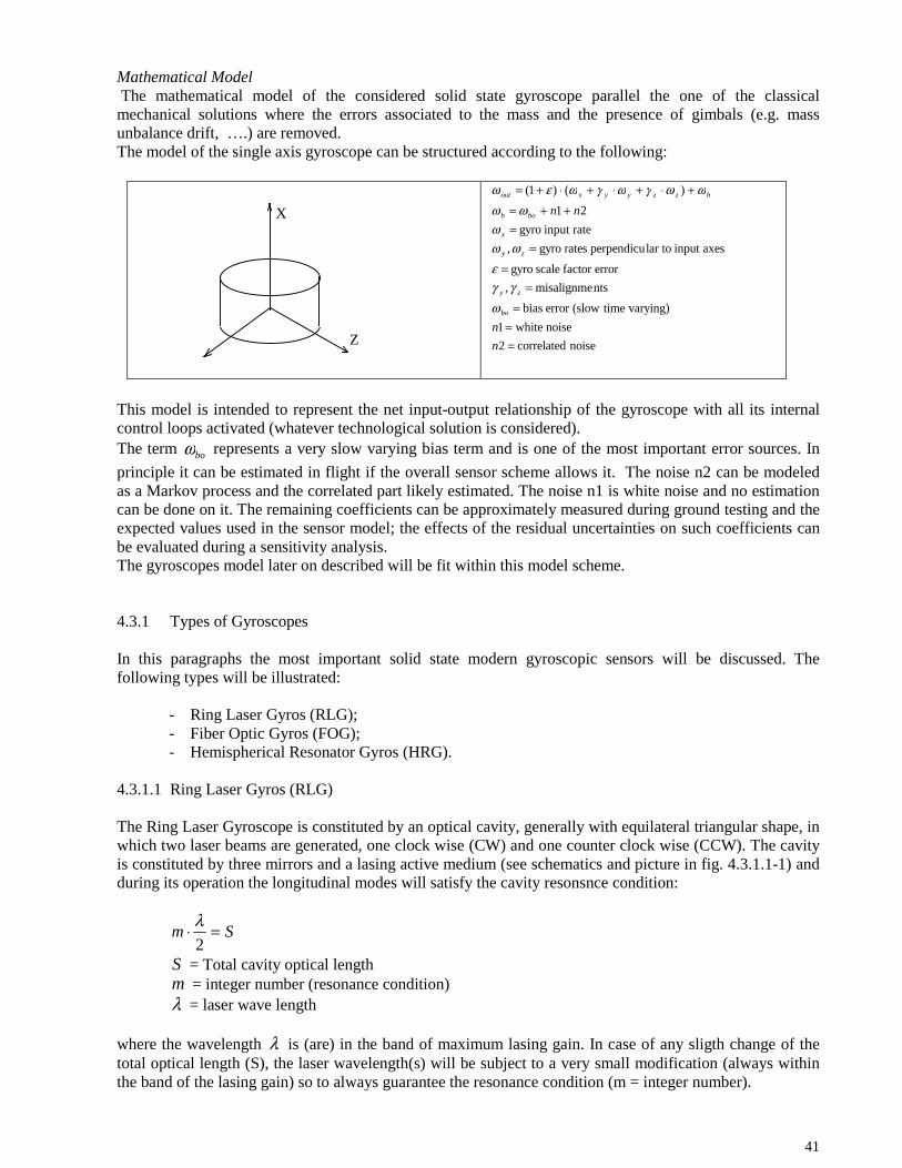
41

Mathematical Model The mathematical model of the considered solid state gyroscope parallel the one of the classicalmechanical solutions where the errors associated to the mass and the presence of gimbals (e.g. massunbalance drift, ….) are removed.The model of the single axis gyroscope can be structured according to the following:

X

Z

noise correlated2

noise white1

varying) time(slowerror bias

ntsmisalignme,

errorfactor scale gyro

axesinput lar toperpendicu rates gyro,

rateinput gyro

21

)()1(

===

==

==

++=

+⋅+⋅+⋅+=

n

n

nn

bo

zy

zy

x

bob

bzzyyxout

ωγγ

εωω

ωωω

ωωγωγωεω

This model is intended to represent the net input-output relationship of the gyroscope with all its internalcontrol loops activated (whatever technological solution is considered).The term boω represents a very slow varying bias term and is one of the most important error sources. In

principle it can be estimated in flight if the overall sensor scheme allows it. The noise n2 can be modeledas a Markov process and the correlated part likely estimated. The noise n1 is white noise and no estimationcan be done on it. The remaining coefficients can be approximately measured during ground testing and theexpected values used in the sensor model; the effects of the residual uncertainties on such coefficients canbe evaluated during a sensitivity analysis.The gyroscopes model later on described will be fit within this model scheme.

4.3.1 Types of Gyroscopes

In this paragraphs the most important solid state modern gyroscopic sensors will be discussed. Thefollowing types will be illustrated:

- Ring Laser Gyros (RLG);- Fiber Optic Gyros (FOG);- Hemispherical Resonator Gyros (HRG).

4.3.1.1 Ring Laser Gyros (RLG)

The Ring Laser Gyroscope is constituted by an optical cavity, generally with equilateral triangular shape, inwhich two laser beams are generated, one clock wise (CW) and one counter clock wise (CCW). The cavityis constituted by three mirrors and a lasing active medium (see schematics and picture in fig. 4.3.1.1-1) andduring its operation the longitudinal modes will satisfy the cavity resonsnce condition:

Sm =⋅2

λ

S = Total cavity optical lengthm = integer number (resonance condition)λ = laser wave length

where the wavelength λ is (are) in the band of maximum lasing gain. In case of any sligth change of thetotal optical length (S), the laser wavelength(s) will be subject to a very small modification (always withinthe band of the lasing gain) so to always guarantee the resonance condition (m = integer number).

42

Fig. 4.3.1.1-1 Schematics and picture of a Ring Laser Gyroscope (ZLG =Zero Lock Gyroscope)

When the gyroscope rotates around its input axis, a difference in the optical path arise for the CW andCCW beams (basically this is due to the constancy of the speed of light and the fact that the mirrors inrotation ‘approaches one of the two beams’ and are ‘moving away with respect to the other’). The twobeams will then result in having a slight different laser frequency.Taking into account the geometry of the cavity, such a difference in frequency results into:

Sc

fAf

⋅⋅⋅Ω⋅=∆ 4

where:

f∆ = Difference in frequency between the CW and CCW beams

Ω = Gyroscope angular velocity

A= Area subtended by the triangular shape of the cavity

f = Beams average frequency

c = Speed of light

S = Cavity optical length = 3 L (L= laser side)

In fig. 3.2.1.1-1 is also shown a method for deriving the output of the Laser Gyroscope. In the example oneof the mirrors is partially transmitting so a very small portion of the CW and CCW beams pass through.One of the two beams is subject to a small angular rotation θ (obtained in this case by means of a prismwith an apex of not exactly 90°). When the beams are recombined at a surface of a detector they will forman interference pattern:

- if the gyroscope angular velocity Ω is zero then the interference pattern is stationary;- if the gyroscope rotates the interference pattern moves across the detector at a speed

proportional to the angular velocity and with a direction of movements indicating the directionof the angular velocity.

The most critical technological issue to solve, associated to the utilisation of the Ring Laser Gyroscopes, isthe so called Lock-In and its effect is shown in fig. 4.3.1.1-2. Each of the two laser beams reaching themirrors, although mostly reflected, is partially scattered back into the opposite travelling beam. If thedifference in frequency is very small (typically at the very low angular velocity) the CW and CCW beamslock together tending to null the difference in frequency. This will lead to a zero output even with a nonzero input angular velocity. Different techniques have been evaluated and tested since the beginning oflaser gyroscopes development to progressively overcome the lock-in (which was indeed the very basiclimiting factor on performances). Some of such techniques are herebelow illustrated:

Mechanical ditherThis technique consists in mechanical dithering the laser block case at high frequency (and lowamplitude) around the input axis via a very stiff suspension spring actuated by a piezoelectricsystem. The result is a gyro that has an alterating biased input (‘far from zero input’), superimposedto the true gyro input, but during the crossing of the zero dither speed. The readout prism andprocessing electronics can be implemented so to have an output signal that accurately represent thetrue gyro input rate free from dither. The penality is the introduction of random noise and somebadwidth limitation.

43

Faraday cellThis technique consists in placing in the laser cavity a magnetic active optical material (plus otheroptical elements) whose index or refraction can be modified by the application of a magnetic field.The modification of the index of refraction can be made different for the CW and CCW beams. Thedifferential change in the speed of light is equivalent to a differential modification of the opticalpath length between the two beams. This gives raise to a difference in the laser frequency for thetwo beams (similar to a controllable input bias rate); the output can then be processed to removethe biasing.

Fig. 4.3.1.1-2 Laser Gyro uncompensated lock-in effect

Magnetic mirrorThis technique consists in applying to one of the three mirrors a magnetic sensitive coating. Byapplying a suitable magnetic field to such coating a differential phase shift is introduced betweenthe CW and CCW beams. This is equivalent a differential path length change around the cavity forthe two beams. This again gives raise to a difference in the laser frequency for the two beams seenas a bias; the output can then be processed to remove the biasing.

The specific detailed solutions utilised by the manufactures to compensate the lock-in are proprietary sincesuch solutions can control the real performances for this type of gyros.The inertial platforms based on RLG zero-lock technology are today very performing.

4.3.1.2 Fiber Optic Gyros

The schematics of a fiber optic gyroscope, and the basic relationship for phase difference, is shown in fig.4.3.1.2-1. The light from a laser source is split (at a splitter) in two beams entering, in opposite directions,the two ends of a fiber optic wounded in a coil. The two counter rotating beams emerges from the ends ofthe fiber optic after a certain time and recombine, by means of the beam splitter, to a suitable detector(arranged as a fringe counter). If the optic coil is not rotating the difference in phase of the two beams at thecounter will be zero. If the coil is subject to an input rotation rate then time of permanence of the twocounter rotating beams in the coil will be slightly different one from the other giving raise, at the fringecounter, to a certain phase difference. The counting of the fringe pulses provides the input rotation rate.

λπ

⋅⋅Ω⋅⋅⋅=∆Φ

c

NA8= Phase difference where:

=A Area of the coil Ω= Input rotation rate N= Number of fibre turns C= Speed of light λ= Laser wavelength

Fig.4.3.1.2-1 Schematics of a Fiber Optic Gyroscope

44

The Fiber Optic Gyroscopes, although originally developed for commercial application and industry, aregaining interest also for space applications. Their performances are not yet to the levels reached by the RLGand HRG (described in the next paragraph).

4.3.1.3 Hemispheric Resonator Gyro

The Hemispherical Resonator Gyro is based on the inertial property of a standing vibration wave at the rimof a hemispherical body. Indeed it has been noted that the location of a vibration pattern at the rim of ahemispherical shell precesses, relative to a reference fixed to the shell body, as a constant factor of the inputrotation. The measurement of precession rate provides a measure of the input speed rate. Fig. 4.3.1.3-1shows an HRG resonator and HRG gyroscope.

Fig. 4.3.1.3-1 HRG components (Litton)

4.3.2 Ring Laser Gyro platform

A very performing RLG based platform is the LN-100S (Litton). The platform is based on the followingmain features:

- 4 Zero Lock Laser Gyros;- suitable for LEO and GEO orbits with a Rad-hard of 100 Krad;- dual processing electronics and dual power supply;- 1553, RS422 interfaces;- equipped with accelerometers.

The main features of such a platform are reported in Fig. 4.3.2-1With reference to the mathematical model previously described, and to above table, the following are noted:

- the contribution to gyro scale factor (ε) and bias error slow varying (ωbo) are clearly identified- the rate white noise (n1) is the contribution called ‘angle random walk’;- the rate correlated noise (n2) is zero;- the term named ‘noise equivalent angle’ of tab. 3.2.2-1 is not to add-up to the rate noise budget;- the misalignments are not declared; they can be evaluated for sensitivity (if necessary).

Fig. 4.3.2-1 Main features of the LN-100S RLG Zero-Lock Gyro platform (Litton)

45

4.3.3 Hemispherical Resonator Gyro platform (Litton)

A very performing HRG based platform is the SIRU (Litton). The platform (see fig. 4.3.3-1) is based on thefollowing main features:

- 4 Hemispherical Resonator Gyros;- suitable for earth orbits and deep space missions, Rad-hard of 100 Krad;- dual processing electronics and dual power supply;- 1553, RS422 interfaces;- optionallly equipped with accelerometers.

The mai features of such a platform are reported in Fig. 4.3.3-1

Fig. 4.3.3-1 Main performances of the SIRU HRG platform (Litton)

The platform is available with two standard of gyroscopes, the moderate performance and the highperformance.With reference to the structure of mathematical model previously described, and to above table, thefollowing are noted:

the contribution to gyro scale factor (ε) and bias error slow varying (ωbo) are clearly identified the rate white noise (n1) is the contribution called ‘angle random walk’; the rate correlated noise (n2) is present and could be modeled as a first order Markov process based

on the term named ‘angle white noise’ of fig. 4.3.3-1 indeed seen as a noise (on the integral of therate) with constant power spectral density within the stated bandwidth;

the term named ‘noise equivalent angle’ of fig. 4.3.3-1 is not to add-up to the rate noise budget; the misalignments are not declared; they can be evaluated for sensitivity (if necessary).

4.4 Orbit Position Sensors

As already evidenced the Pointing S/C alignment relative to the Target S/C can be performed with no needof accurate position control or position knowledge. It has however been assumed to keep the S/Cs aroundtheir nominal allocated coordinates within a range less than 1000 (m) and the position knowledge shallsuffice to guarantee this recovery.Four methods of position measurements are presented:

- GPS utilisation in high orbits;- Radiolocalisation methods;- Laser Ranging.

GPS based autonomous navigation at high orbits ([64][65]) is still in an evolving phase. GPS satellitessignals are directed toward the earth with a broadcast pattern that is slightly wider than the planet. Thus aGEO S/C at the opposite side of the earth can, with a proper receiver, collect and process the GPS

46

‘spillover’ signals. Two main issues affect the whole performances: the weakness of the signals received bythe user S/C and the time of coverage.Special receivers/antennae need be used in GEO capable to deal with the very low level signals receivedand capable to cope with the limited visibility by implementing the functions of ‘orbital navigation’, aKalman Filter based navigation system which combine GPS measurments with orbital force models. Tocope with the visibility problems in GEO the correct approach would be, for future scenarii, to extend theL-band coverage for example by means of dedicated antenna onboard GPS satellites.Some GPS receivers capable to operate in GEO are being developed. As an example Alcatel TOPSTAR3000 GPS can provide the position with an accuracy of 100 m (3D, 1σ).

Radiolocalization method are developed with the aim to provide all weather, continuous visibilityautonomous navigation features. These methods utilize transmitters/receivers on board the S/C and anappropriate arrangement of ground stations.The basic measurements performed are related to range and range rate of the S/C with respect to the groundstations. At least two frequencies are involved in the trasmission in order to allow for atmospheric relatedcorrections. Based on this, the S/C position can in principle be computed by a real time on board navigator.For an indication of achievable performances with these method two developments are mentioned.PRARE system [66] (Precision Range and Range-rate Equipment) has been a national development of theFederal Republic of Germany. The predicted ranging accuracy is given as 5-10 cm.DORIS-DIODE [67] (Doppler Orbitography and Radiopositioning Integrated by Satellite – DeterminationImmediate d’Orbite par Doris Embarqueé) is a system being developed by CNES and can provide on boardreal time 3D positioning. Some of these system have already flown (e.g. SPOT 4), others are planned to fly(e.g. Jason 1).The predicted 3D positioning accuracy is in the range of 30 cm (rms).The degree of applicability and adaptability of the radiolocalisation methods to GEO orbit need be dulyassessed based on the specific system/application.

Satellite Laser Ranging is certainly one of the most precise technique for satellites position determination.Depending on the application considered centimetric accuracy can be achieved.In the specific case the S/Cs, equipped by retroreflectors, are nominally geostationary and their accuratelocalization from ground is facilitated; the approach could be to compute the 3D coordinates on ground andthen transmit them to the S/Cs. Time delay, dynamics, … can be taken into account prior to datatransmission.The ground satellite laser ranging stations can be fixed (like Matera Range Station [68]) or transportable(like the French FTLRS [69]).Based on the S/Cs assigned orbital positions and to cope with the visibility uncertainties associated to theweather conditions, an appropriate number of transportable ground station can support the in orbitexperiment. The stations can be placed at well selected locations characterized by favourable weatherconditions. Based on data from Topex/Poseidon and Lageos, the transportable FTLRS stations can provideaccuracies in the order of 2 cm.

To support the simulation phase it can certainly be assumed an orbit position determination, for the S/Csinvolved in the experiment (in GEO), with the following range of performances:

- residual error (biasing) < 0.05 m- noise < 0.05 m rms

which can be achieved by laser ranging or by laser ranging supported by radiolocalization.It is however noted that biasing in the order of tens of meters will not affect the experiment performances.

47

5. Actuators

Concerning the actuators the following approach has been considered.During Target acquisition and keeping the relative attitude control is performed by µN class lowdisturbance thrusters. Three types have been evaluated: Pulsed Plasma, Colloidal, FEEP (Field EmissionElectric Propulsion).The thrusters for ultraprecise control need to have the following basic features:

- very high exaust speed (to minimise the amount of propellant to be stored and handled);- controllable thrust down to < 1 µN (and up to some onehundered µN;- extremely low minimum controllable impulse (to minimise the subsequent motion drift);- electrically throttable with no mechanical moving parts;- low noise during continuous operations;- no propellant sloshing associated to the operations.

Of the different type of electric propulsion system presented (which are all in study or under developmentfor advanced space applications like control of interferometric platforms, drag free control, …), the FEEPbased technology seems to present really outstanding performances which render them potential candidatesfor the most advnced missions.They are yaken as reference for the evaluation of dynamic performances in the considered mission scenario.Reaction wheels, for attitude control, have been also evaluated but judged too noisy for the jitters inducedabove 1 Hz even if of high balance degree and isolation mounted.

Position recovery is assumed performed by mN class thrusters of classical type and performancesequivalent to xenon thrusters have been assumed. During the core scientific phase all thrusters are excluded.

5.1 Pulse Plasma Thrusters

Pulsed Plasma Thrusters (PPT) are electromagnetics type thrusters which utilise solid Teflon as propellant([59] and [53]).The operative principle (see also fig. 5.1-1 for a PPT schematics) is the following:

- the Teflon at the surface layer is made ablating by means of a large voltage potential whichproduces a breakdown; the arc passing through the ablated teflon ionises it;

- the formed ions are accellerated downstream by means of the Lorentz force induced by themagnetic field associated to the arc;

- the accelleration is furthermore enhanced by a thermal gas dynamic effect.

The PPT mode of operation is of pulsed type: it consists of continuous repetitions of interval with thrustand of interval with no thrusts. The basic performance parameters are the Impulse bit deliverable Ibit(µN.s), the Pulse Repetition Rate PRR (Hz) and the specific Impulse during the periods of thrusts Isp (s).

Fig. 5.1-1 Schematics of PPT Thruster

48

The processes involved are very complicated and most of the available models are of empirical type.The average thrust can be modulated by acting on the Ibit (which generally is in the range 20-2000 µN.swith some attempts to go toward 2 µN.s) and the PRR ( which generally does not exceed 10 Hz). Also theIbit to Ibit variability can be of a problem for high precision applications (this variability tend to increase bylovering the Ibit ). PPT thrusters have flown many times.

Fig. 5.1-2 shows a PPT thruster system EO-1 PPT made od two single thrusters and the relevant typicalperformances.

Fig. 5.1-2 Example of PPT thruster ([59])

5.2 Colloidal Thrusters

Colloidal thrusters ([53]) are based on the principle to extract ionized droplets/particles or atoms from anelectrolitic liquid, or ionic liquid, and accellerate them by means of strong electric fields. A schematicprinciple of colloidal thruster on needle type is shown in fig. 5.2-1.

Fig 5.2-1 Schematic of colloidal thruster of needle type

These needle thrusters can be clustered together to form groups or blocks that can be separately activated.This feature combined with the possibility to regulate the accellerating voltage allows to reach a continuousthrottling capability through a wide range of thrusts.It is however noted that the activations of a group or block is not immediate at command but require sometime to allow the formation of the fluid menisci into the cone-jets and to emit droplets.Reference characteristics achievable by colloidal thrusters are summarized herebelow:

49

Thrust (one needle) = 0.13 (µN)Isp = 509 (s)Power (one needle) = 0.25 (mW)Clustering possibility = some hundereds

One manufacturing technology that can allow the implementation of a large number of emitters array persurface area is MEMS Micro Electronic Mechanical System [60]. The small features achievable withMEMS would allow to reduce the thrusters size also allowing to reduce the needed voltages. An example ofthrusters batch of this type is shown in fig. 5.2-2.

Fig. 5.2-2 Example of a cluster of colloidal thrusters [60]

To date these colloidal thrusters have been developed at laboratory level but likely never flown.

5.3 FEEP Thrusters

FEEP technology, at an excellent development stage, is here considered (see also ref. [ 51], [52], [53], [54])and the main features discussed.

FEEP thrusters are designed to utilise as propellant liquid phase metal stored locally to the thruster; twodesign have so far been performed:

- cesium based thrusters (in development at Centrospazio-Pisa);- indium based thrusters (in development by the Austrian Research Centers).

In fig. 5.3-1 is shown the schematics of a cesium based thruster. It consists of a slit shaped emitter whichalso locate the propellant reservoir, the accelerator (or extractor) and the neutraliser. The approximate slitdimensions are in the order of 1-2 µm in height and between 1 mm to several centimeters in width. Theaccelerator is placed in front of (but very near) the emitter slit and the neutraliser in front of the acceleratorto null the net emitted charge. Basically positive cesium ions are generated et the emitter, acceleratedtoward the accelerator and then neutralised in the exaust phase.

The actuator is throttable and the performances can be tailored by adjusting:- the emitter voltage (Ve)- the accelerator voltage (Va)- the choice of slit width

For the slit type design, the following relations provide an estimate of thrust (F) and specific impulse (Isp):

( )( )(s) Impulse SpecificVe122.3Isp

(N)Thrust V0.9167)-1E(23)-1E (1.666NF

(Volts) Voltages Va Ve,

mm 5by normalizedlenght Slit

0011.0e

=⋅=

=⋅⋅⋅⋅⋅⋅⋅=

==

+⋅ ae VVe

N

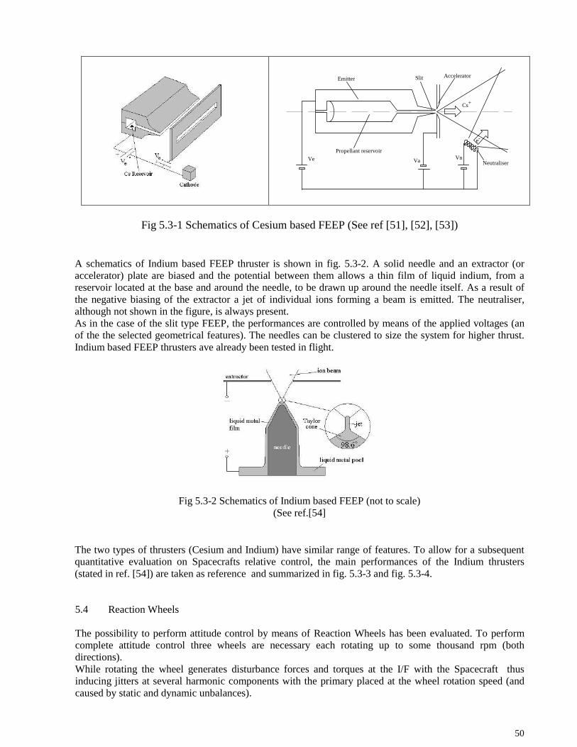
50

Emitter Slit Accelerator

Propellant reservoir

Neutraliser

Cs+

e-

VnVaVe

Fig 5.3-1 Schematics of Cesium based FEEP (See ref [51], [52], [53])

A schematics of Indium based FEEP thruster is shown in fig. 5.3-2. A solid needle and an extractor (oraccelerator) plate are biased and the potential between them allows a thin film of liquid indium, from areservoir located at the base and around the needle, to be drawn up around the needle itself. As a result ofthe negative biasing of the extractor a jet of individual ions forming a beam is emitted. The neutraliser,although not shown in the figure, is always present.As in the case of the slit type FEEP, the performances are controlled by means of the applied voltages (anof the the selected geometrical features). The needles can be clustered to size the system for higher thrust.Indium based FEEP thrusters ave already been tested in flight.

Fig 5.3-2 Schematics of Indium based FEEP (not to scale)(See ref.[54]

The two types of thrusters (Cesium and Indium) have similar range of features. To allow for a subsequentquantitative evaluation on Spacecrafts relative control, the main performances of the Indium thrusters(stated in ref. [54]) are taken as reference and summarized in fig. 5.3-3 and fig. 5.3-4.

5.4 Reaction Wheels

The possibility to perform attitude control by means of Reaction Wheels has been evaluated. To performcomplete attitude control three wheels are necessary each rotating up to some thousand rpm (bothdirections).While rotating the wheel generates disturbance forces and torques at the I/F with the Spacecraft thusinducing jitters at several harmonic components with the primary placed at the wheel rotation speed (andcaused by static and dynamic unbalances).

51

Fig 5.3-3 Summary of performances for Indium based FEEP (see ref.[54])

Thrust Resolution

Thrust noise Power Spectral Density

Fig 5.3-4 Summary of performances for Indium based FEEP (see ref.[54])

52

Fig. 5.4-1 illustrates the wheel ITHACO-E [61], evaluated in the frame of the Next Generation SpaceTelescope program (NGST) Yardstick mission design. In tab. 5.4-1 are reported some of the mainspecifications of the wheel in particular the static mass unbalance and the dynamic mass unbalance.

Fig. 5.4-1 Schematic of the ITHACO-E Reaction Wheel [61]

Tab. 5.4-1 Main specification of the ITHACO-E Reaction Wheel [61]

The disturbance effects on the relative alignment of the Pointing S/C to Target S/C has been evaluated,considering the static and dynamic unbalances, for one reaction wheel with characteristics similar to theITHACO-E. The wheel speed range evaluated has been 180-950 rpm and a vibration attenuation factor hasbeen considered at the mount to simulate the presence of vibration suppressors. The attenuation factor hasbeen derived as the response of a Low Pass passive system (an approach similar to [62]) with 2 Hzbandwidth.

The results are shown in Tab. 5.4-2. The simulation evidence pointing jitters in the range 1E-3 to 1E-4(arcsec) which corresponds to approximately 0.05 to 0.005 (m) at the target surface. The presence of at leastthree wheels plus the disturbances induced by other causes like bearings, motors and drive electronics,further increase such jitters which turn out very large in comparison the the one achievable withmicrothrusters control (which will turn out orders of magnitute lower). Furthermore during the scientificportions of the missions the thrusters can be switched off while the wheel cannot unless with a de saturationlike procedure not compatible with the mission itself.

53

NRW=3 rps (180 rpm)RAWF=1

NRW=3 rps (180 rpm)RAWF= 0.5598

NRW=6 rps (360 rpm)RAWF=1

NRW=6 rps (360 rpm)RAWF= 0.2077

NRW=15.8 rps (948 rpm)RAWF=1

NRW=15.8 rps (948 rpm)RAWF= 0.0520

CASE: REACWA DT=0.01(s) TTOT=120(s) REG=0.5(s) Reaction wheel (HST class) simul08rwh

Tab. 5.4-2 Example of disturbances (at one wheel speed) on relative attitude caused by reaction wheel

0 500 1000 1500 2000 2500 3000 3500 4000 4500 50000

0.2

0.4

0.6

0.8

1

1.2x 10

-3

rela

tive

gam

ma

fft (

arcs

ec)

freq (Hz) shown range 1-50 Hz

0 500 1000 1500 2000 2500 3000 3500 4000 4500 50000

0.2

0.4

0.6

0.8

1

1.2x 10

-3

rela

tive

gam

ma

fft (

arcs

ec)

freq (Hz) shown range 1-50 Hz

0 500 1000 1500 2000 2500 3000 3500 4000 4500 50000

0.2

0.4

0.6

0.8

1

1.2

1.4

1.6

1.8x 10

-3

rela

tive

gam

ma

fft (

arcs

ec)

freq (Hz) shown range 1-50 Hz

0 500 1000 1500 2000 2500 3000 3500 4000 4500 50000

1

2

3

4

5

6x 10

-4

rela

tive

gam

ma

fft (

arcs

ec)

freq (Hz) shown range 1-50 Hz

0 500 1000 1500 2000 2500 3000 3500 4000 4500 50000

0.5

1

1.5

2

2.5x 10

-4

rela

tive

gam

ma

fft (

arcs

ec)

freq (Hz) shown range 1-50 Hz

0 500 1000 1500 2000 2500 3000 3500 4000 4500 50000

0.2

0.4

0.6

0.8

1x 10

-4

rela

tive

gam

ma

fft (

arcs

ec)

freq (Hz) shown range 1-50 Hz

54

6. Main External Disturbances

6.1 Generalities

In this chapter the major sources of ‘disturbance’ acting on a Spacecraft are reviewed and commented. Theterm ‘disturbance’ includes the torques and forces acting on the Spacecraft with the sole exclusion of themain gravity force acting at the Spacecraft center of mass and generated by the one nominal sphericalsimmetric attractive body. A summary of such disturbances, for a generic orbit, is reported in tab. 6-1.

Disturbance effect on S/CDisturbance type Torque Force

Remarks

Solar RadiationPressure

yes yes Level of disturbances depend on the optical/geometricalproperties of the S/C surfaces. Torques depend on S/Cshape non symmetries and optical mismatch.

Solar and Lunarattraction

yes These effects depend on Moon-S/C-earth and Sun-S/C-earth relative position. Lowering the height of the orbitthe effects reduce. This is the strongest disturbance atGEO.

Earth geopotentialdistortions

yes Different contributing terms exist. Effects stronglyreduce with orbital heigth.

Gravity gradienttorques

yes They depend on inertial balancing of the Spacecraft andon it orientation with respect the local gravity. Theyreduce with orbital heigth and, in principle, can berendered very small ‘by design’.

Tidal effects yes These effects are induced by the movements of the‘fluid’ parts of the integrated earth/oceans/athmospheresystem. The disturbances strongly reduce with heigth.

Athmospheric drag yes yes Predominant at LEO orbits. Drops very quickly withorbit heigth.

Meteoroid impacts yes yes The effects can be evaluated based on meteoroids fluss-mass models and result in very low disturbances.

Tab. 6-1 Main disturbances actin on an orbiting Spacecraft

In the specific case considered, the mission taken as reference is conceived in GEO orbit, the S/Cs arealways under attitude control and undergo position recovery procedure every 2-3 hours (at most), the strictcontrol performed appearing very robust. Above listed disturbances are reviewed in the next paragraphs forthe GEO case, with the exception of the atmospheric drag, in order to asses them for the purpose of aquantitative evaluation of the S/Cs performances.General reference is done to documents [46], [47] and [48] while more specific references are shownwhere necessary.

6.2 Solar radiation pressure

Let us consider an elementary surface perpendicular to the sun direction and illuminated by it. The photonsenergy flux from the sun (solar energy flux or irradiance) hits the surface and undergo a change inmomentum. This creates the so called solar radiation pressure, and therefore a force on the surface.

55

Such a a force is of the following type (see also ref. [49], [50]):

( )

( )

=⋅=

=

==⋅≅=

+===

=

=⋅⋅=

pressure radiation Average N/m 104.55 c

F : toleads This

)(W/m nsfluctuatioflux energy Solar F

1AU)(at flux energy solar Average W/m 1365 F

(m/s) 103 light of Speedc

FF )(W/mflux energy Solar F

)(msun the toexposedsection (cross) Surface S

)reflectantfully is surface thecasein 2

absorbant,fully is surface thecasein (1 2-1 range in theC

pressureradiation the todue (N) Force SCF

26-0

2d

20

8

d02

2

p

p c

F

The resulting force is directed along the sun-surface line and opposite to the sun and will be formed by anaverage value plus fluctuations.Concerning the fluctuations they are the contributions from time and spatial variations of small scale solarsurface structures integrated over the solar disk. From low to high frequencies, surface inhomogeneitiessuch as sunspots and faculae, convective structures and their evolution, produce the ‘noise’ contribution tothe solar energy flux.An example of solar irradiance fluctuation is shown in fig. 6.2-1 (both as time history and power spectrum).The following considerations are worth being pointed out.

Average effectsIn spite of a good knowledge of the average energy flux, the average force can only be computed to anapproximate degree. Indeed two factors contribute to its uncertainty.

- The first factor, and the less important, is related to the actual S/C shape far from being a flatsurface pointing to the sun. This imply, assuming fully known the local optical and geometricalproperties of the surface, a complex integration over the spacecraft surface leading to an‘average force’ estimation which will have components also perpendicular to the sun’sdirection.

- The second factor, more important that the above one, is related to the knowledge of thespacecraft optical properties (basically leading to the estimate of the coefficient Cp in thereported formulation). Such properties change during the operative lifetime of the spacecraftalso by some tens per cent causing a similar amount of uncertainty in the average forcecomputation.

Concerning the average force we can therefore say that the radial component could be in the range of 4.55

– 9.9 ( 2/ mNµ ) times the cross sectional area of the spacecraft and that there will be a transversalcomponent, not easily definable, lower than the radial one but not far as order of magnitude (e.g. 10%).Also a disturbing torque will appear depending on the geometrical and optical non symmetries of the

spacecraft. Disturbing torques in the range 0.5 – 1 ( 2/ mmN ⋅µ ) could be considered even for symmetricgeometries.

Sun

Surface (S)

Force

56

If not compensated the radial component of the force will tend to render the orbit eccentric; the orbital timeperiod would be approximately maintained with no neat energy introduction:

Earth

Perigees

Apogees

From Sun

Fluctuation effectsThe data collected on irradiance fluctuation are covering the 0.01 Hz range approximately.

Time History - SoHO/VIRGO Ref.[49] Power Spectrum - SoHO/VIRGO Ref.[49])

Power Spectrum trend Ref.[50]

Fig. 6.2-1 Example of solar irradiance fluctuation

It however appears that the fluctuation spectrum goes beyond such low values even if the quantitativebehaviour seems not available.

For our evaluation purposes we can consider two limit power spectra cases:

First irradiance limit spectra

White noise with a constant PSD of about ( )

Hz

22W/m 5 .0 hereafter shown:

57

IrradianceLog PSD

0

-1

-2

FrequencyLog Hz

0-1-2 1-3

This corresponds to an infinite rms disturbance not realistic but in principle acceptable forphysically low pass band systems and very easy to be modeled;

Second irradiance limit spectraWhite noise, with PSD of 10 W/m², filtered with a first order filter ( τ = 1000 s)

IrradianceLog PSD

1

0

-1

FrequencyLog Hz

-1-2-3 0-4 +1

-2

This corresponds to a more realistic disturbance with an rms value of approximately 0.1 (W/m2); thishowever constitute a worst case of rms since the actual value seems to be in the range of 0.05 (W/m2).At frequencies in the order of 10 Hz the disturbance seems very low; it has anyway to be remembered thatalso the observed phenomena are extremely low.

Assuming a criteria similar as for the average effects, the fluctuation effects (considered generated fromwhite noise with PSD of 10 W/m²) will apear at spacecraft level as:

radial fluctuation forces in the order of 0.00035 - 0.0007 ( 2/ mNµ rms) times the cross sectionalarea of the spacecraft and transversal fluctuation forces with the transversal effects in the 10%range of the radial;

torque disturbances (in pitch and yaw) in the range of 0.000035 – 0.00007 ( 2/ mmN ⋅µ rms)times the cross sectional area of the spacecraft (for spacecraft in the meters size).

The treatment of the solar radiation pressure effects as ‘pseudo potential’ is not applicable to our situation.

6.3 Solar and Lunar attraction

The perturbing force experienced by an earth orbiting satellite caused by a perturbing body (the sun or themoon) is expressed as the body attraction on the satellite minus the body attraction on the earth, for themoon this is hereafter shown.

58

( )m

mm

m

mmeffm r

r

rr

rrf

µµ−

−−

=

where:

( )

(m)center earth .r.t position w vector Satellite

(m)center earth .r.t position wtor center vecMoon

/m 104.896constantMoon

plane) orbital satellite not the is which on the lays (Note

(N/kg) direction n'' thealongcomponent force Perturbing

(N/kg) direction r'' thealongcomponent force Perturbing

(N/kg) massunit per satellite on the acting force perturbing Effective''

2312

,

,

,

==

⋅≅=

=

=

=

=

r

r

s

rrf

f

f

f

m

m

meff

nm

effnm

effrm

effm

µ

The expression for the forces components is:

( )

ΦΦ−=

−Φ=

mm

meffnm

mmm

meffrm

r

r

rf

r

r

r

r

rf

sin cos 3

cos 3

2,

2

2,

µ

µ

with a similar expression holding for the sun.

As can be noted the forces depend on the angle Φ (note: is not on the satellite orbital plane) which changesdepending on the motion of satellite, earth and perturbing body with periodicities hereafter described.The maximum values for the forces components are (where such maximums do not occure simultaneously):

=

=

=

=

N/kg 46.2

N/kg 28.3

N/kg 44.5

N/kg 26.7

max,

max,

max,

max,

µ

µ

µ

µ

effns

effrs

effnm

effrm

f

f

f

f

6.4 Earth geopotential distortions

A generic S/C orbiting the earth in a nominal circular orbit (e = o) and with nominal zero inclination (i = 0),is subject to a primary perturbing potential of the following type (with respect to a perfectly spherical bodywith spherical symmetric density distribution):

MoonΦ

Earth

effnmf ,

Satellite

r

mr

effrmf ,

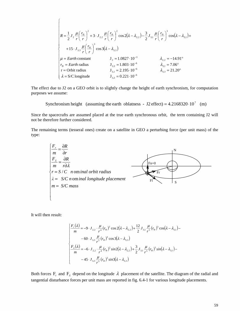
59

( ) ( )

( )

°=⋅=⋅=

==

°=⋅==°−=⋅==

−

⋅+

+−

−−

⋅+

=

−

−

−⊕

−

⊕

⊕⊕⊕

20.21

10221.0J

10195.2J

longitude S/C

radiusOrbit r 06.7 10803.1J radius

91.14 100827.1J constant

3cos15

cos2

32cos3

2

1

3,3

63,3

63,1

1,36

2,2

2,23

2

3,3

3

3,3

1,3

3

1,32,2

2

2,2

2

2

λλ

λλµ

λλµ

λλµλλµµ

Earthr

Earth

r

r

rJ

r

r

rJ

r

r

rJ

r

r

rJR

The effect due to J2 on a GEO orbit is to slightly change the height of earth synchronism, for computationpurposes we assume:

(m) 102168320.4effect) J2 - oblatnessearth the(assumingheight mSynchronis 7⋅=

Since the spacecrafts are assumed placed at the true earth synchronous orbit, the term containing J2 willnot be therefore further considered.

The remaining terms (tesseral ones) create on a satellite in GEO a perturbing force (per unit mass) of thetype:

===

∂∂=

∂∂=

S/C massm

menttude placeinal longi S/C nλ radiusinal orbitnCSr

r

R

m

Fr

R

m

Fr

om

om /λ

λ

N

S

Fn=0

Fr

Fl

It will then result:

( ) ( ) ( ) ( ) ( )

( ) ( )( ) ( ) ( ) ( ) ( )

( ) ( )

−⋅−

−−+−⋅⋅−=

−⋅−

−−+−⋅⋅−=

⊕

⊕⊕

⊕

⊕⊕

3,33

53,3

1,33

51,32,22

42,2

3,33

53,3

1,33

51,32,22

42,2

345

2

326

3cos60

cos2

122cos9

λλµ

λλµλλµλ

λλµ

λλµλλµλ

λ

sinrr

J

sinrr

Jsinrr

Jm

F

rr

J

rr

Jrr

Jm

Fr

Both forces rF and λF depend on the longitude λ placement of the satellite. The diagram of the radial and

tangential disturbance forces per unit mass are reported in fig. 6.4-1 for various longitude placements.

60

It is noted that for satellites holding a given assigned longitude (e.g. with accuracies in the rough range oftypical GEO stellite station keeping control) the forces per unit mass can be considered constant around thekept position.

0 50 100 150 200 250 300 350 400-1

0

1x 10

-7

placement degrees

Fr/m

0 50 100 150 200 250 300 350 400-1

0

1x 10

-7

placement degrees

Fl/m

Fig. 6.4-1 Diagram of the radial and tangential disturbance forces per unit mass for various longitudeplacements (geosynchronous orbit)

6.5 Gravity gradient torques

For a GEO satellite the gravity gradient related torques normally can be neglected from a short termdynamic analysis. In the scenarios here considered such torques can however induce variation in attitudeswhich can impact the permanence time on target. It is then necessary to quantify this effect in order to setsome limits on the maximum allowed inertia unbalance.Fig 6.5-1 quantify the gravity gradient torques effect.

k

j

i

GEO orbit+v bar

r TGG= Gravity Gradient Torque= 3 n² [(C-B)ef i+(A-C)df j+(B-A)ed k]

where:

i j k = Spacecraft principal axis of inertia

r = d i + e j + f k = Local gravity direction

A, B, C, Spacecraft principal M.o.I.

n = Orbit angular speed

Fig. 6.5-1 Gravity gradient torques

61

In the specific experiment scenario considered the principal axis of the Pointing S/C are assumed orientedalong the Nominal Alignment Frame with a relative error at most in the arcsec order. With reference to thelocal gravity only the pitch angle (γ ~ 5°) plays a role since this angle is needed to optically align to thedistant Target S/C.In these conditions the k axis is perpendicular to the orbital plane (f = 0) and the torque would limit to:

TGG = 3 n² (B-A)ed kwhere:d = cos(γ) e = -sin(γ) and with γ = pitch angle

To keep limited the torque effects, given a certain pitch angle, it is then necessary to have the S/C balancedin terms of inertia. Assuming to accept a residual torque in the order of 10% of the unbalance torqueprovided by the solar pressure unbalance it turns out that the moment of inertia (A and B) should differ byno more than 25 (kg*m^2) which can be achieved by balancing methods. In such conditiong the gravitygradient torque would approximately be 5*1E-8 (Nm).

6.6 Tidal effects

Tidal disturbances are gravity field variations associated to mass redistribution of the integratedearth/ocean/athmosphere system. The masses displacement and redistribution is caused primarily by theMoon and Sun differential effects on the ‘fluid’ parts of the integrated system.As an example fig. 6.6-1 sketches the ocean tide at two combinations of the Moon-Sun relative position[63].

Fig. 6.6-1 Sketchs of the ocean tide caused by Moon and Sun

The gravity field variations induced by tides depend on both position and time and for the relevantmeasurements very precise instrumentation is needed.Tab. 6.6-1 summarizes the order of magnitude for the gravity fields variation experienced nearby the earthsurface. It appears that the major disturbance effect is caused by earth tides followed by the contributionsfrom oceans, ground water, athmosphere and polar motions. Taking into consideration that 1m/s2 = 108

Gals disturbances in the order of 10-6 m/s2 are expected at earth surface and they will reduce very muchincreasing the distance from earth.

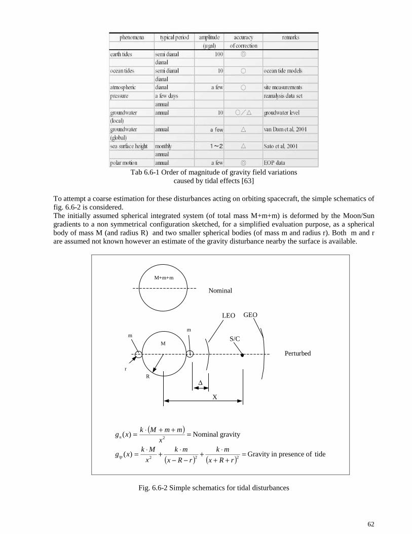
62

Tab 6.6-1 Order of magnitude of gravity field variationscaused by tidal effects [63]

To attempt a coarse estimation for these disturbances acting on orbiting spacecraft, the simple schematics offig. 6.6-2 is considered.The initially assumed spherical integrated system (of total mass M+m+m) is deformed by the Moon/Sungradients to a non symmetrical configuration sketched, for a simplified evaluation purpose, as a sphericalbody of mass M (and radius R) and two smaller spherical bodies (of mass m and radius r). Both m and rare assumed not known however an estimate of the gravity disturbance nearby the surface is available.

∆R

X

M+m+m

M

mm

LEO GEO

S/C

r

Nominal

Perturbed

( )

( ) ( ) tideof presencein Gravity )(

gravity Nominal )(

222

2

=++

⋅+−−

⋅+⋅=

=++⋅=

rRx

mk

rRx

mk

x

Mkxg

x

mmMkxg

tp

n

Fig. 6.6-2 Simple schematics for tidal disturbances

63

A generic spacecraft at distance ‘x’ from the earth center will experience a variation of the gravity fieldpassing from the nominal condition ‘n’ to the tide perturbed conditions ‘tp’ given by:

( ) ( )onsperturbati related Tide

2)(

222=⋅⋅−

++⋅+

−−⋅=−=

x

mk

rRx

mk

rRx

mkggxg ntpδ

For spacecrafts nearby GEO (x ~ 6*R) and LEO (e.g. ∆=600 km) the following is expected:

onsperturbati related Tide)(

onsperturbati related Tide200

)(

2

2

=∆⋅≅

=⋅⋅≅

mkLEOg

R

mkGEOg

δ

δ

Passing from LEO to GEO a very strong reduction is present (thousands of times). Since the disturbances inLEO are not greater than the ones measured at the surface, then the tidal effects on a spacecraft placed inGEO will be very much smaller than the other type of disturbances (which add up to an approximate rangeof 10-5 m/s2). In the frame of the mission control scheme considered the tdal effects are neglected.

6.7 Meteoroid impacts

In GEO orbit meteoroids are much more likely to be encountered than orbital debris and are the onlypenetration hazard in outer space.For this evaluation, reference is made to Grun model of meteoroid flux reported in fig. 6.7-1.

Fig. 6.7-1 Grun meteoroid flux model

The diagram provides, for each generic value of particle mass m, the total number of particles (with masslarger than the mass m) hitting the spacecraft per unit reference surface per unit reference time.Assuming for example a flux of particles with speed Vp relative to the spacecraft, the force acting per unitof normal surface can be estimated as:

==

=

=⋅⋅⋅−=

(m/s) speed Particles V

le)(kg/partic mass Particle

)//m(particlesFlux )(

)(N/m surfaceunit per forceImpact

p

2

2

m

smF

dmmdm

dFVP p

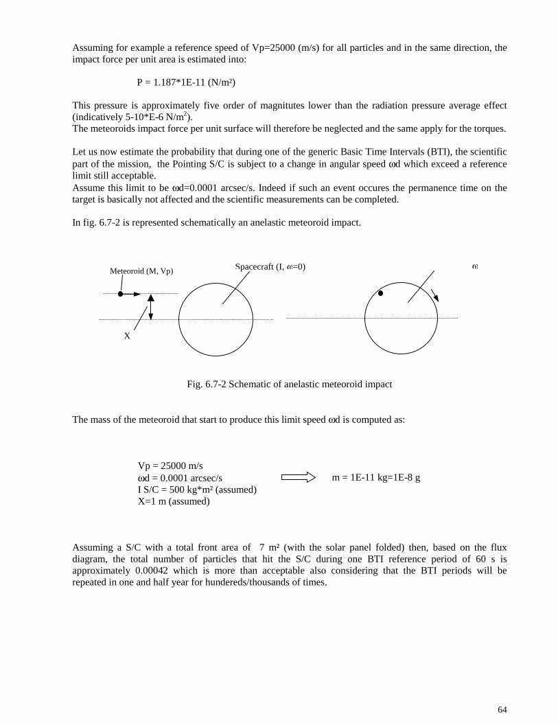
64

Assuming for example a reference speed of Vp=25000 (m/s) for all particles and in the same direction, theimpact force per unit area is estimated into:

P = 1.187*1E-11 (N/m²)

This pressure is approximately five order of magnitutes lower than the radiation pressure average effect(indicatively 5-10*E-6 N/m2).The meteoroids impact force per unit surface will therefore be neglected and the same apply for the torques.

Let us now estimate the probability that during one of the generic Basic Time Intervals (BTI), the scientificpart of the mission, the Pointing S/C is subject to a change in angular speed ωd which exceed a referencelimit still acceptable.Assume this limit to be ωd=0.0001 arcsec/s. Indeed if such an event occures the permanence time on thetarget is basically not affected and the scientific measurements can be completed.

In fig. 6.7-2 is represented schematically an anelastic meteoroid impact.

Fig. 6.7-2 Schematic of anelastic meteoroid impact

The mass of the meteoroid that start to produce this limit speed ωd is computed as:

Vp = 25000 m/sωd = 0.0001 arcsec/sI S/C = 500 kg*m² (assumed)X=1 m (assumed)

m = 1E-11 kg=1E-8 g

Assuming a S/C with a total front area of 7 m² (with the solar panel folded) then, based on the fluxdiagram, the total number of particles that hit the S/C during one BTI reference period of 60 s isapproximately 0.00042 which is more than acceptable also considering that the BTI periods will berepeated in one and half year for hundereds/thousands of times.

ωMeteoroid (M, Vp) Spacecraft (I, ω=0)

X

65

7. MODELLING AND EVALUATION OF PERFORMANCES

In this paragraph the relative control performances of the Pointing S/C with respect to the Target S/C, forthe experimental configuration identified at previous paragraph 4, will be presented as evaluated by meansof a dedicated simulations.The paragraph is organised according to the following scheme:

- reference frames definition and Pointing S/C structural scheme;- modelling (dynamic and measurements);- control schemes;- simulation results (organised per phases).

and the results are reported and discussed for the main operational phases of:- target acquisition and keeping under thrusters control;- scientific phase;- position recovery.

7.1 Reference Frames definition and Pointing S/C structural scheme

The reference frames defined for the simulation are shown in fig 7.1-1 and fig. 7.1-2 and herebelowdescribed:

),,,( TTTT kjiO

= Target S/C nominal orbital frame;

TO placed at the Target S/C nominal location;

Tj

oriented along the nominal +V bar;

Ti

radial from the earth centre directed outward;this frame is fully defined and rotates at a uniform rotation speed (around the z axis)of OMEGAN.

),,,( PPPP kjiO

= Pointing S/C nominal orbital frame;

PO placed at the Pointing S/C nominal location

Tj

oriented along the nominal +V bar;

Ti

radial from the earth centre directed outward:this frame is fully defined and rotates at a uniform rotation speed (around the z axis)of OMEGAN.

),,,( APAPAPAP kjiO

= Nominal alignment frame at Pointing S/C (rotation of the Pointing S/C nominalorbital frame aroung the z axis);

APO placed at the Pointing S/C nominal location (coincident with PO )

Aj

oriented to nominal Target;this frame is fully defined (by GEO distance nd S/Cs nominal separation distanceD) and rotates at a uniform rotation speed (around the z axis) of OMEGAN.

),,,( ATATATAT kjiO

= Nominal alignment frame at the Target S/C (rotation of the Target S/C nominalorbital frame around the z axis);

ATO placed at the Target S/C nominal location (coincident with TO )

ATj

oriented as APj

;this frame is fully defined (by GEO distance and S/Cs nominal separation distanceD) and rotates at a uniform rotation speed (around the z axis) of OMEGAN.

66

)( ARj

= Required alignment direction;this direction is defined by means of the true positions of the Pointing and TargetS/Cs

),,,( SSSS kjiO

= Pointing S/C outer structural frame;

SO placed at the outer structure C.M.

Sj

oriented along the ‘forward’;

Si

oriented along the ‘outer radial’ direction;

this frame is defined w.r.t. the Nominal alignment frame ),,,( AAAA kjiO

by meansof:

- a small translation (XS,YS,ZS);- a small rotation (ALFAS, BETAS, GAMMAS - yaw, bank, pitch).

),,,( oooo kjiO

= Pointing S/C inner optical platform frame;

oO placed at the optical platform C.M.

oj

oriented along the ‘forward’ optical axis;

oi

oriented along the ‘outer radial’ direction.

this frame is defined w.r.t. the Pointing S/C outer structural frame ),,,( SSSS kjiO

by means of:- a small translation (XO,YO,ZO);- a small rotation (ALFAO, BETAO, GAMMAO - yaw, bank, pitch).

The Pointing S/C structural scheme is also illustrated in fig. 7.1-2 and is composed of:- inner optical platform carrying the high accuracy optical payload (relative attitude sensor

interferometer, pointing laser, narrow field of view star tracker, metrology system) andgyroscopes;

- an outer structural frame carrying all remaining typical S/C sub systems (propulsion, power,thermal, TT&C, OBDH);

- two short appendages representing e.g. solar panels folded and locked, antennas, ….. .

The inner optical platform and the outer structure are connected by means of 6 springs (3 linear, 3 angular)and 6 dampers (3 linear, 3 angular). Each of the the two appendages are connected to the outer structuralframe by means of 2 springs (1 linear, 1 angular) and 2 dampers (1 linear and 1 angular).The Pointing S/C state vector is described by 38 components (32 needed to describe positions and speedsof the assumed masses and 6 needed as extensions, to describe the non white noise of the solar radiationpressure fluctuations).

67

ATj

ATi

Pointing S/C NominalOrbital Frame ---------

Pointing S/C

Target S/C NominalOrbital Frame -------

Target S/C

PiPj

Ti

Tj

GEO ORBIT

+ V bar

+ V bar

ND

Earth

OP,OAP

Nominal AlignmentFrame

APi

APj

Required Pointing Direction

ARj

Fig. 7.1-1 Pointing S/C and Target S/C nominal orbital frames (not to scale)

OT, OAT

Nominal AlignmentFrame (at Target)

TD

68

Fig. 7.1-2 Pointing S/C outer structural frame, optical frames and appendages (schematis only)

oi

oj

oo

Target Optical Platformsi

sj

Target Outer Structure

sO

Optical axis

oO

Os

Outer structure and Optical platform connected byequivalent 6 axis springs (3 rotational, 3 translational)

and 6 axis dampers (3 translational, 3 rotational).

sj

sk

Short appendages each connected with 2 axissprings (1’x’ rotational, 1 ‘y’ translational) and

2 axis dampers (1 ‘x’ rotational, 1’y’translational), rigid otherwise

69

7.2 Dynamics (modelling and measurements)

For the objectives of the present analysis the system composed by the Pointing S/C and the Target S/C hasbeen linearized and modelled around the nominal configuration. Different models have been derived and,in the final configuration, the following set of equations have been considered:

→+⋅+⋅+⋅+⋅=

→+⋅+⋅+⋅+⋅=

→⋅+⋅+⋅+⋅+⋅+⋅+⋅+⋅=

•

•

dynamicsspacecraftetT

thrtsfluxTBtesttTBperbtTBpostarATpostar

measurmentspacecraftingPo

nvecfvecztxtMCoffpospMCoffvMCpstvMCymeas

dynamicsspacecraftingPo

pnovDtoggGGBpsfvBpepvBpbpvBbrtvBpntvBpstvApstv

arg

654

int

),( 3421

int

1765431

The Target S/C has been assumed as an independently controlled platform whose co ordinates (xt, yt, zt)enter the measurement equations of the Pointing S/C. In turn the control loop of the Pointing S/C inject theinformation on the Target S/C position into the Pointing S/C dynamics via the regulator equations. Theobjective is to keep the Pointing S/C as much as possible relatively aligned to the Target S/C and with theminimum possible relative jitter.

A brief description of the vector and matrices involved in above equations is hereafter reported and on thecomposition of the main state and measurement vectors is given.

Pointing Spacecraft Dynamics

)138( xpstv = Pointing spacecraft state vectorThe pointing spacecraft state vector is summarised in tab. 7.2-1. and the following points are remarked:

- the spacecraft dynamics (structural frame, optical platform, left and right appendages) is

described in the nominal alignment frame ),,,( APAPPAAP kjiO

which is not an inertial framebut rotates at a nominally constant angular rate;

- the alignment of the spacecraft with respect to this frame is at most within some tens ofarcseconds and the relative very small rotations can be added;

- the six disturbances related to solar radiation pressure noise (3 forces, 3 torques) are included inthe state vector since they are modelled starting from white noise.

)3838( xA = Pointing spacecraft dynamic matrixThe Pointing spacecraft dynamic matrix encompass the following terms:

- inertia and ‘proximity motion’ of centre of masses;- inertia and Euler equations for rotation around centre of masses;- terms associated to stiffness and damping among modelled parts;- terms associated to the shape filter to produce grey solar radiation fluctuations.

70

==

==

==

==

======

=+=+=+

=+=+=+

=======+=+=+

=+=+=+======

=

appendageleft of rate yaw ALFAP2D

appendageleft of yaw ALFAP2

appendageleft of speedy YP2D

appendageleft of coordinatey YP2

appendageright of rate yaw ALFAP1D

appendageright of yaw ALFAP1

appendageright of speedy YP1D

appendageright of coordinatey YP1

z along noise torquepressureradiation RPMNZ

y along noise torquepressureradiation RPMNY

xalong noise torquepressureradiation RPMNX

z along noise force pressureradiation RPFNZ

y along noise force pressureradiation RPFNY

xalong noise force pressureradiation RPFNX

frame platform optical theof ratepitch GAMMAODGAMMASD

frame platform optical theof ratebank BETAODBETASD

frame platform optical theof rate yaw ALFAODALFASD

frame platform optical theofpitch GAMMAOGAMMAS

frame platform optical theofbank BETAOBETAS

frame platform optical theof yaw ALFAOALFAS

frame structural spacecraft theof ratepitch GAMMASD

frame structural spacecraft theof ratebank BETASD

frame structural spacecraft theof rate yaw ALFASD

frame structural spacecraft theofpitch GAMMAS

frame structural spacecraft theofbank BETAS

frame structural spacecraft theof yaw ALFAS

frame platform optical theof speed z ZODZSD

frame platform optical theof speedy YODYSD

frame platform optical theof speed x XODXSD

frame platform optical theof coordinate z ZOZS

frame platform optical theof coordinatey YOYS

frame platform optical theof coordinate x XOXS

frame structural spacecraft theof speed z ZSD

frame structural spacecraft theof speedy YSD

frame structural spacecraft theof speed x XSD

frame structural spacecraft theof coordinate z ZS

frame structural spacecraft theof coordinatey YS

frame structural spacecraft theof coordinate x XS

(38x1) pstv

Tab. 7.2-1 pstv - Pointing spacecraft state vector

71

Concerning linearisation some notes are herebelow evidenced.

1. The equation for linear proximity motion of a puntiform body around an orbital frame are of the form(with the symbols and conventions shown in the picture):

=+−=

+−=

++=

⋅⋅

⋅⋅⋅

⋅⋅⋅

frameofspeedangular

fzz

fxy

fxyx

z

y

x

2

32

2

2

ωω

ω

ωω

They are already in a linearized form (around the point O of coordinates x=0, y=0, z=0) and hold fordisplacements from the reference point O limited to some kilometres. This is indeed the case of ourconcern. Above written equations have to be adapted to describe the motion around a frame inclinedwith respect to the one shown in the picture but still remain linear.

2. The equation for angular motion of a rigid body around the center of mass are of the form (Eulerequations):

+−⋅⋅−=⋅

+−⋅⋅−=⋅

+−⋅⋅−=⋅

⋅⋅⋅⋅

⋅⋅⋅⋅

⋅⋅⋅⋅

MzIxIyIz

MyIzIxIy

MxIyIzIx

)(

)(

)(

βαγ

αγβ

βγα

Since for the phases of motion considered the body is always aligned with respect to the nominalalignment frame by less than some arcsec (and in the really important phases by less than fractions ofarcsec) and with angular rates relative to this frame of much less than fractions of arcsec/s then theequations are linearised around the condition:

======

===⋅⋅⋅

) om ( 0 0

, , 0 0 0

, , 0 0 0

zy framealignmentinalnofspeedangularmeanswhich

ratepitchraterollrateyawrelative

pitchrollyawrelative

x ωωωωγβα

γβα

and take the form:

=⋅

+−⋅−=⋅

+−⋅−=⋅

⋅⋅

⋅⋅

⋅⋅

MzIz

MyIzIxIy

MxIyIzIx

γ

ωβ

ωα

)(

)(

3. The stiffness damping behaviour has been assumed linear.

)16( xpntv = Pointing spacecraft nominal thrust vectorThe Pointing spacecraft nominal thrust vector is the thrust vector command (Fx, Fy, Fz, Mx, My, Mz) asgenerated by the position regulator and encompasses, in general, the three forces and three torques actions.This command vector in given in input to the thrusters drive electronics which command the thrustersassumed fixed to the outer structural frame of the spacecraft.

O

GEO orbit

x

Gun S/C

y

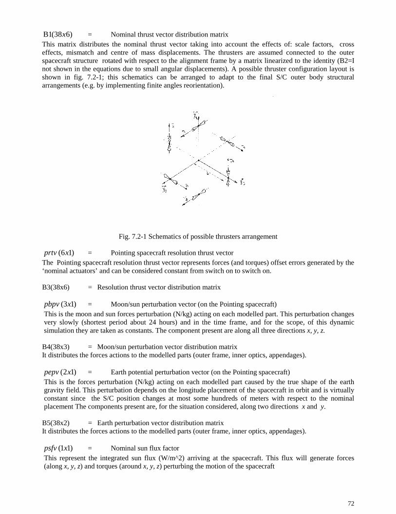
72

)638(B1 x = Nominal thrust vector distribution matrixThis matrix distributes the nominal thrust vector taking into account the effects of: scale factors, crosseffects, mismatch and centre of mass displacements. The thrusters are assumed connected to the outerspacecraft structure rotated with respect to the alignment frame by a matrix linearized to the identity (B2=Inot shown in the equations due to small angular displacements). A possible thruster configuration layout isshown in fig. 7.2-1; this schematics can be arranged to adapt to the final S/C outer body structuralarrangements (e.g. by implementing finite angles reorientation).

Fig. 7.2-1 Schematics of possible thrusters arrangement

)16( xprtv = Pointing spacecraft resolution thrust vectorThe Pointing spacecraft resolution thrust vector represents forces (and torques) offset errors generated by the‘nominal actuators’ and can be considered constant from switch on to switch on.

B3(38x6) = Resolution thrust vector distribution matrix

)13( xpbpv = Moon/sun perturbation vector (on the Pointing spacecraft)This is the moon and sun forces perturbation (N/kg) acting on each modelled part. This perturbation changesvery slowly (shortest period about 24 hours) and in the time frame, and for the scope, of this dynamicsimulation they are taken as constants. The component present are along all three directions x, y, z.

B4(38x3) = Moon/sun perturbation vector distribution matrixIt distributes the forces actions to the modelled parts (outer frame, inner optics, appendages).

)12( xpepv = Earth potential perturbation vector (on the Pointing spacecraft)This is the forces perturbation (N/kg) acting on each modelled part caused by the true shape of the earthgravity field. This perturbation depends on the longitude placement of the spacecraft in orbit and is virtuallyconstant since the S/C position changes at most some hundreds of meters with respect to the nominalplacement The components present are, for the situation considered, along two directions x and y.

B5(38x2) = Earth perturbation vector distribution matrixIt distributes the forces actions to the modelled parts (outer frame, inner optics, appendages).

)11( xpsfv = Nominal sun flux factorThis represent the integrated sun flux (W/m^2) arriving at the spacecraft. This flux will generate forces(along x, y, z) and torques (around x, y, z) perturbing the motion of the spacecraft

73

B6(38x1) = Nominal sun flux force/torque distribution matrix.This matrix generates (and distributes) forces and torques to the spacecraft starting from the radiationpressure present at GEO orbit. It takes into account an average reflection and shape factors to distinguishbetween different directions and apply these effects to the outer structural frame.

)12( xtogg = Gravity gradient torques vectorThis represent the torques (around z) generated by the gradient of gravity on the two major parts of thepointing spacecraft (the outer structure, inclusive of appendages, and the optical platform).

B7GG(38x2) = Gravity gradient torques distribution matrix.This matrix distributes the torques to the outer structure (inclusive of the effects of appendages) and to theinner optical platform.

)112( xpnov = Overall (white) noise vectorThis vector encompasses all white noise sources acting on the system and include the thrust vector randomnoise (6x1) and the white generators (here taken 6x1) for the generation of the solar radiation noisefluctuations.

D1(38x12) = Noise vector distribution matrix.It distributes the thrusters noise to the outer structure of the spacecraft and generates the solar radiationfluctuations (forces and torques) for filtering and later distribution.

The integration of the dynamic equation of the Pointing Spacecraft is performed by utilising transitionmatrix tecqnique with series expansion up to the 11th order. A comparative evaluation has been performedby using an expansion up to the 18th order and a relative accuracy on angles better than 6 significative digitshas been achieved with integration steps of 0.01 (s) both for maximum values and jitters (>1Hz).

Pointing Spacecraft Measurement

The pointing spacecraft measurment vector (summarized in tab. 7.2.-2) gather the different types ofmeasurments assumed available. The following remarks apply:

- the configuration of the measurment vector changes based on the assumed sensors configuration;- the measurments include the nominal part, offsets, scale factors, the noise;- the following basic sensors are assumed:

interferometric relative attitude sensor; high accuracy star tracker; pointing spacecraft position determination (based on SLR satellite laser ranging,

transponding techniques, GPS); rate gyros.

- the relative yaw and bank (of the the pointing spacecraft optical platform w.r.t the target spacecraft)

are defined w.r.t. the required alignment direction vector ARj

and the signs are in agreement with

the nominal alignment frame )( APAR jj

≅ ;

- the absolute yaw of the pointing spacecraft optical platform is defined in the ),,,( APAPAPAP kjiO

frame;- the pointing spacecraft position are referred to the outer structural frame. It does not need to be

specified for optical platform frame since the accuracy of interest is in the several centimetre rangeand not in the micron or sub micron range; we can assume such measurements relate to the outerstructural frame. The pointing spacecraft position is referred to the nominal alignment frame;

- the attitude rates are absolute and relates to the optical platform frame ),,,( oooo kjiO

.

)19( xymeas = Measurement vectorThis vector encompasses all measurments as summarized in tab.7.2-2.

74

=========

=

rateangular z absolute platform optical

rateangular y absolute platform optical

rateangular x absolute platform optical

position z spacecraft ZS

positiony spacecraft YS

position x spacecraft XS

pitch absolute S/C target toplatform optical S/C pointing ABANK

bank relative S/C target toplatform optical S/C pointing RPITCH

yaw relative S/C target toplatform optical S/C pointing RYAW

)19(

OMEGAZ

OMEGAY

OMEGAX

xymeas

Tab. 7.2.-2 ymeas - Pointing spacecraft Measurment Vector

MC1(9x38) = Measurement distribution matrix.This matrix support the distribution of the state vector into measurements and encompasses terms including:

- scale factors on relative yaw (partial), relative pitch (partial), absolute bank;- scale factors on absolute angular rate yaw, absolute angular rate pitch (partial), absolute angular rate

bank;- effects of true separation distance TD (partial).

)16( offv x = Offset vector #1This vector encompasses the offset relative to the measurements of: relative yaw, relative pitch, absolutebank, absolute angular rate yaw, absolute angular rate bank, absolute angular rate pitch.

MC2 (9x6) = Offset vector distribution matrix.This matrix distributes the offset vector #1

)13( ofposp x = Offset vector #2This vector encompasses the offset relative to the measurements of: pointing spacecraft position

MC4 (9x3) = Offset vector distribution matrix.This matrix distributes the offset vector #2

)13( fvec x = Forcing vectorThis vector, which can be seen a ‘forcing term’ into the equation, encompasses the Target Spacecraftposition as it evolves from its dynamic (injection point into the Pointing Spacecraft system) and the angularrate ω of the orbital frame.

MC3 (9x3) = Forcing vector distribution matrix.This matrix support the distribution of the forcing state vector into measurements and encompasses termsincluding:

- scale factors on relative yaw (partial), relative pitch (partial), absolute angular rate pitch;- effects of true separation distance TD (partial).

)19( xnvec = Overall measurement (white) noise vectorThis vector encompasses all white noise sources acting on the measurements and include relative yaw,relative pitch, absolute bank, position measurements(x, y, z) absolute angular rate (yaw, bank, pitch).

Concerning linearisation some notes are here below evidenced.

1. The true distance TD is a function of the nominal distance ND and the two involved spacecrafts position,In general it has the following form:

75

222 )()()( ZPZTXPXTYPYTNDTD −+−+−+=

Taking into account the nominal separation distance involved (10000 km) and the maximum spacecraftsoff position (some hundereds of meters), it can be taken:

NDTD ≅

since this approximation injects an inaccuracy in the relative parameters determination (relative yaw,relative pitch) at most in the order of 1:10000 (i.e. 0.001 arcsec at the very high relative attitudes of 10arcsec).

The Pointing S/C measurement vector is assumed available at a frequency of 2 Hz which is compatible withthe update rate of the high accuracy star trackers and the interferometric relative attitude sensor.The rate gyros information are however available also at high update rates (e.g. >100 Hz).

Target Spacecraft Dynamics

The target spacecraft dynamics is related to the computation of the Target S/C co ordinates (XT, YT, ZT).The attitudes of the Target S/C are assumed controlled by means of an attitude sensor of performancescomparable to a high resolution Star Tracker (and therefore in the range of few arcsec in roll and pitch) andare not modelled.

)16( xpostar = Target spacecraft state vector

The target spacecraft state vector is summarized in tab.7.2-3. and the following points are remarked:

- the spacecraft dynamics is described in the nominal alignment frame at

target ),,,( ATATPTAT kjiO

which is not an inertial frame but rotates at a nominally constantangular rate;

- the same consideration concerning linearisation of proximity motion as described for thepointing S/C apply.

======

=

speed z S/C target ZTARD

speedy S/C target YTARD

speed x S/C target XTARD

position z S/C target ZTAR

positiony S/C target YTAR

position x S/C target XTAR

)16( xpostar

Tab. 7.2.-3 postar - Target spacecraft state vector

)66( xAT = Target spacecraft dynamic matrixThe Target spacecraft dynamic matrix model the target as a single rigid body and encompass the followingterms:

- ‘proximity motion’ of centre of mass;)13( xperbt = Moon/sun perturbation vector (on the Target spacecraft)

This is the moon and sun forces perturbation (N/kg) acting on the target S/C. This perturbation changes veryslowly (shortest period about 24 hours) and in the time frame, and for the scope, of this dynamic simulationthey are taken as constants. The present component are along all three directions x, y, z and differ ‘slightly’from the equivalent components on the pointing S/C.

76

B4T(6x3) = Moon/sun perturbation vector distribution matrixIt distributes the forces actions to the S/C body.

)12( xtestt = Earth potential perturbation vector (on the Target spacecraft)This is the forces perturbation (N/kg) acting on the S/C body caused by the true shape of the earth gravityfield. This perturbation depends on the longitude placement of the spacecraft in orbit and is virtuallyconstant since the S/C position changes at most some hundreds of meters with respect to the nominalplacement The present components are, for the situation considered, along two directions x and y and differ‘slightly’ from the equivalent components on the pointing S/C.

B5T(6x2) = Earth perturbation vector distribution matrixIt distributes the forces actions to the S/C body.

)11( xsflux = Nominal sun flux factorThis represent the integrated sun flux (W/m^2) arriving at the target spacecraft. This flux will generateforces (along x, y, z) and torques (around x, y, z) perturbing the motion of the spacecraft

B6T(6x1) = Nominal sun flux forces distribution matrix.This matrix generates (and distributes) forces to the spacecraft starting from the radiation pressure present atGEO orbit. It takes into account an average reflection and shape factors to distinguish between differentdirections and apply these effects to the S/C body.

)16( xthrt = Thrust vector (per unit mass)This vector encompasses the control forces acting on the target S/C. It is written with no distribution matrixand has the following components (0, 0, 0, Fx/MT, Fy/MT, Fz/MT).

The performed simulations encompass three modalities of target position evolution:- target in position free drift mode (in this case the x, y, z position control is off and thrt =0) and

controlled attitude (with respect to the alignment frame);- target in position and attitude free drift mode;- target assumed kept still at XT=YT=ZT=0 and controlled attitude (with respect to the alignment

frame). In this case no simulation on target is performed.

In all conditions the target position and attitude jitters are considered in the overall relative budget:- in the first case position and attitude jitters are estimated based on the position and attitude jitters of

the pointing S/C when in position drift and controlled in attitude (projecting the performances with asensor similar to an high resolution star tracker and with thrusters of xenon type);

- in the second case position and attitude jitters are taken similar to position and attitude jitters ofpointing S/C in full drift mode;

- in the third case position and attitude jitters are taken similar to the position and attitude jitters ofthe pointing S/C in the steady phase at the end of position recovery (position and attitude controlledby a sensor of performance similar to an high resolution star tracker and by thrusters of xenon type).

The integration of the dynamic equation of the Target Spacecraft is performed by utilising transition matrixtecqnique with series expansion up to the 11th order. A comparative evaluation has been performed by usingan expansion up to the 18th order and no difference has been noticed between positions with integrationsteps of 0.01 (s).

77

7.3 Control schemes

In this paragraph the basic control schemes utilised for the simulation are introduced. In all schemes thecontrol is achieved by implementing control loops based on six independent PID regulators dedicated to :

- two relative attitudes (Pointing to Target S/Cs relative alfa and gamma angles);- one absolute attitude (beta, however relative to the local alignment frame);- three positions coordinates (X opt, Y opt, Z opt however relative to the local alignment frame).

The control analysis has been carried out by considering two types of thrusters system utilised in differentperiods of the mission:

- a very accurate micronewton class thrusters (limited to 100µN and 300µNm)

dedicated to the relative target acquisition (and keeping) phase and:

- millinewton class thrusters (limited to 20mN and 60mNm,

dedicated to the position recovery phase.

During the relative target acquisition phase the position control is not active (OFF) since it is not needed bythe mission and because the micronewton thrusters would not anyhow be able to perform it and only the tworelative attitudes and the absolute attitude are controlled. The utilisation of millinewton thrusters wouldinduce strong disturbances in the relative pointing/alignment.During the position recovery phase the micronewton thrusters are not active (OFF) since they would not beof any effect while the control is performed in absolute mode (however relative to the local alignmentframe) in all six coordinates.

7.3.1 Control scheme for relative target acquisition (and keeping)

The basic control scheme utilised is shown in fig. 7.3.1-1 with the position control switched OFF. It is basedon direct sensors information with specific filtering implemented on the most noisy parameters. Two timingare considered in the simulation: an interval DT for the simulation of the dynamics and an interval REG forthe simulation of the control loops and the attitude/position sensors acquisition (relative attitudeinterferometer, high accuracy star tracker and position measurement system even if not used in this scheme).The gyros are sensors which allow data availability at high frequency and it has then been assumed for thesesensors a faster acquisition rate (than 1/REG) followed by strong filtering.Typically DT=0.01 (s), with sensitivity testing carried out at lower times (e.g. 0.0025 s, 0.001 s) and REG =0.5 (s) with sensitivity testing carried out at larger times (e.g. 2 s). It is noted that although the commandedforces (Fxc, Fyc, Fzc) are zero, the actual forces exterted by the thrusters are not zero because of thepractical imperfections involved (positioning, alignments, mismatch,…).All the features described in the model presented at paragraph 7.2 are implemented.

The gains of the regulators have been selected based on two approaches: tuning of gains with ‘trial and test’(e.g. placement and regulation of proportional gains followed by placement and regulation of derivativegains and integral gains with iterations) and utilisation of deterministic optimum control techniques [58] toderive proportional and derivative gains of comparable regulators.

In order to assess the capabilities achievable through the support of an in line dynamic filtering, a variant ofcontrol scheme utilising a Kalman Filter has been prepared [57] [58]. The schematics is shown in fig. 7.3.1-2and makes use of a basic sensor acquisition all done at the ‘REG’ interval.

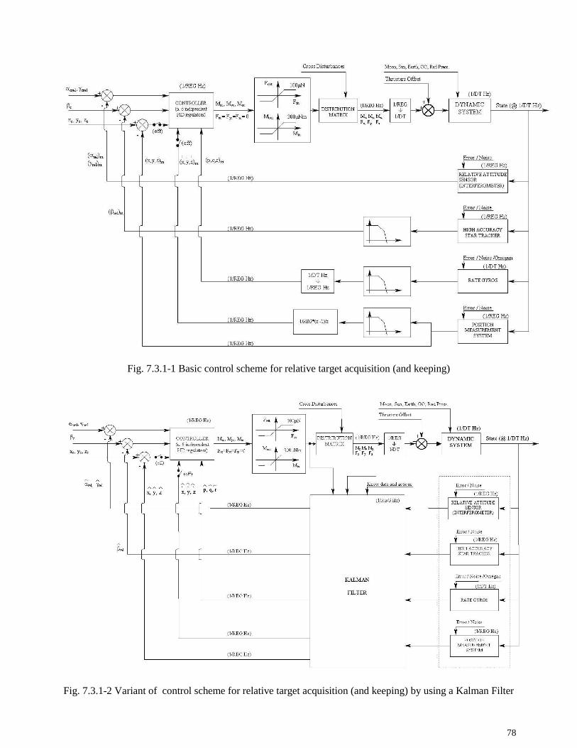
78

Fig. 7.3.1-1 Basic control scheme for relative target acquisition (and keeping)

Fig. 7.3.1-2 Variant of control scheme for relative target acquisition (and keeping) by using a Kalman Filter

79

Concerning the KF implementation, the following considerations are noted:

a) the system distribution matrices, the radiation pressure average disturbances, the measurement matrixand some forcing parameter in the measurment equation have been implemented with inaccuracies;indeed 21 perturbing parameters are present directly affecting the attitude behaviour;

b) the system dynamic matrix have been assumed strongly perturbed in two primary stiffnesses to simulatepartial structural failure during launch.

Above perturbations have two types of effects at the level of performances considered: the perturbations oftype a) create some relative attitude offsets (in the order of 0.01 arcsec) in the KF state reconstructionshowing minor sensitivity while the perturbations of type b) are more important and tend to render the KFunstable showing an important sensitivity.

To cope with above situations the following approach have been used:a) the minor offsets have been controlled by implementing an integration action within the KF structure

(see also Fig. 7.3.1-3);b) the strong sensitivity to uncertainties in the dynamic matrix have been controlled by extending the KF to

the uncertain parameters; the KF becomes then non linear so it has been linearized,

Other methods like ‘memory loss’ can indeed control the instabilities due to dynamic matrix uncertaintiesbut the relative attitude errors increase to approximately 0.02-0.03 arcsec and the jitter in the band >1 Hzincreases by a factor of 50 which is to be avoided for the specific application considered.The approach utilised allows a robust estimator with no need of an excessive extension of the filter.The Kalman Filter here implemented has the main scope of noise reduction.

7.3.2 Control scheme for position recovery phase

During the recovery phase large amount of position displacements are to be managed, typically tens orhundereds of meters in the case considered. A control scheme which utilises the final commanded coordinates directly in the control loop can require large time of stabilisation if the control has very limitedaction capabilities (e.g. non linear control caused by weak saturation thresholds like in our case). In suchcircumstances speed limitations may be needed otherwise the regulation action of the PID could requireseveral passages near the final reference coordinates to damp the oscillations. An alternative and moredeterministic approach can be devised taking as examples the ‘trajectory generation techniques’ also used inother branches of engineering (like robotics).With such an approach smooth reference trajectories can be planned with polynomial profiles compatiblewith the characteristics of the actuators and the desired quality of motion. For the specific case a quadraticgeneration has been considered for each of the six controlled co ordinates.The recovery manoeuvers are implemented in two steps (see also Fig. 7.3.2-1 for a generic coordinate S):during the first step speed slow down till zero is achieved, in the second step the position is recovered to thenominal zero coordinate (and zero speed).

For each step the process is the following:- an initial sensor reading is performed;- for each of the coordinates a minimum required manoeuver time is computed compatible to both the

target coordinate and a selectable amount of thrust/torque not to exceed; in such a way a due extraamount of force/torque is still available for the regulation actions (external disturbances compensations,specific regulation, …);

- the longest of the six times is taken as reference and the six profiles are re generated by using thisreference time;

- in such a way the planned maximum forces/torques for each of the nominal generated trajectories will bebelow the allowed limits;

- the six profiles are then passed to the system controller.

80

- +K

- +K+1

[ ]

)1()1(ˆ)1(ˆ

)()1()1()()1(

)1(

)1(ˆ)1()1(ˆ)1(ˆ

)1()1(

)()1(ˆ

1

1

+⋅++=+−⋅+−++=+

↓

+=++⋅−+++=+

+++⋅=++⋅Φ=+

++

++

−

−+−+

+−

kIGIkxkx

ttkzkzkIkI

kz

GkxMkzKkxkx

WGkxMkz

Fkxkx

C

kk

k

Fig. 7.3.1-3 KF modification with a ‘weak’ integrator during the update phase

Fig. 7.3.2-1 Schematics of trajectory generation

The selection of the parameters used for the trajectory profile generation affect primarily the time ofmanoeuvers and the electric power requirements, to a lesser extent the fuel consumption. The gains used inthe control loop, related to the allowed errors during manoeuvers, affect the fuel consumption; optimumdetermined gains from linear theory are considered. However it has to be said that the closed loop systemvery easily becomes non linear (due to the forces saturation) as soon as the manoeuver is tried to be quiker.The approach considered allows anyway to perform stable and reliable recovery.

81

A schematic of control loop for the recovery phase is shown in Fig. 7.3.2-2 and realises the control on allaxes (positions and attitudes). It has been simulated by considering a relative attitude sensor withcharacteristics typical of an absolute high accuracy star tracker and by considering actuators of Xenon typecapable of thrusts level compatible with this type of mission. The obtained performances are representativeof an absolute control in the nominal alignment frame and with the target S/C placed at zero.

Fig. 7.3.2-2 Basic control scheme for the position recovery phase controller

82

7.4 Simulation results

In this paragraph some indicative simulation results are reported and organised per experiment operationalphase:

- target acquisition and keeping under thrusters control;- scientific phase;- position recovery.

7.4.1 Target relative acquisition and keeping under thrusters control

In this phase the alignment of the Pointing S/C on to the Target S/C is achieved and maintained by thePointing S/C via attitude control. The Target S/C is not cooperative: it has just to maintain an attitudeorientation (with respect to the nominal alignement frame) within several tens of arcsec.

Five study cases (out of the whole cases evaluated) are reported and hereafter discussed:

- Case # 1: fast moving target and ‘low’ control gains;- Case # 2: still target with perturbed motion and ‘low’ control gains;- Case # 3: fast moving target and ‘medium’ control gains;- Case # 4: fast moving target with perturbed motion and control by KF with ‘low ‘ gains;- Case # 5: fast moving target with perturbed motion and control by KF with ‘high‘ gains determined

with optimum techniques;

Case # 1: fast moving target and ‘low’ control gains

This case refers to the following situation:- the target spacecraft is in position free drift with high initial speeds conditions; it is assumed in

attitude control mode with respect to the target nominal alignment frame (xenon thrusters and highresolution ST);

- the pointing spacecraft is in position free drift mode with high initial attitude errors; it is in relative totarget attitude mode guided by the information from the interferometric relative attitude sensor andFEEP thrusters;

- the gains of the regulator are classified as ‘low’ since they allow initial a pronounced overshoot;- general features:

Total simulation time =1000(s);Measurement and regulator frequency = 2 Hz;Dynamic time step = 0.01 (s)

The achieved results are reported in fig. 7.4.1-1 a) to f) and the following comments apply:

- fig. 7.4.1-1 a) provides an overview of performances from T=0 (s) except where otherwise indicated.It is noted the initial overshot and a full settlement time of approximately 150 (s);

- fig 7.4.1-1 b) provides the relative performances in time domain from T=700 (s) to T=1000 (s) withsome statistical information. Overall pointing accuracy in the order of (per axis):

relative attitude error (rms) < 0.006 arcsecrelative attitude error (max observed) < 0.013 (arcsec)position on target error (rms)< 0.27 (m)position on target error (max observed) < 0.6 (m)

83

The pointing spacecraft drifts in position by approximately 3 (m) which would grow to about 300(m) in three hours;

- fig. 7.4.1-1 c) provides an overview of the performances in frequency domain (for f >1 Hz) as resultfrom data evaluation from T=900 (s) to T=1000 (s). For the positions a modification of the input filehas been necessary to be able to carry out a meaningful fft.Concerning the Target S/C the jitters in attitudes and displacements can be estimated based onsimulations performed on the pointing S/C when controlled in attitude by means of Xenon thrustersand high accuracy Star Tracker (SENXENHST); considering a safety factor of 10, due to possibleTarget spacecraft structural frequency magnifications, the following can be certainly reached withsuitable gains:

target S/C attitude jitter (rms) < 8.3*1E-5*10= 8.3*1E-4 (arcsec) which induce a sensordisplacement in the order of 4.2*1E-8 (m) for a Target CM to Target sensor distance of 10(m);target S/C position jitter (rms)< 1.1*1E-12*10= 1.1*1E-11 (m)

Such target S/C behaviour do not affect the relative pointing performances at the target sensor planewhich are controlled basically by the attitude related performances of the pointing spacecraft (whichare reported in the figure); per axis they are:

jitter at target sensor plane (rms) (in terms of attitudes)< 1.2*1E-6 (arcsec)jitter at target sensor plane (rms) (in terms of displacements)<5.4*1E-5 (m)= 54 (µm)

- fig. 7.4.1-1 d) provide some other data including the commanded torques (by the control loop). Theangular rate ωx reported shows a non zero sustained value which is due to both the target spacecraftand the pointing spacecraft position drifts;

- fig 7.4.1-1 e) shows the position displacement of the target S/C. It seems a linear function because ofthe assumed high initial speeds; indeed is a parabolic like curve. The final values of displacementsare already indicative of the ones expected after three hours of mission in realistic free motion. Alsoreported are pitch and yaw of the pointing spacecraft relative to the local alignment frame: theychange since the pointing S/C keep tracking of the moving target;

- fig 7.4.1-1 f) report the total fuel consumption for this 1000 (s) mission. Also shown are the electricpower and energy at thrusters electronics input. Assuming this type of control continuously activefor two years the total amount of fuel consumption (e.g. indium or cesium) would be 0.05 (kg).

84

From t=250.51 (s) to T=1000 (s)

Fig. 7.4.1-1 a) Case # 1: fast moving target and ‘low’ control gains;

TARGACQ01TA Simul08finbt inputflex01fint xxx08 prepro02E low gains S/C separation= 10000 (km)DT=0.01 (s) TTOT=1000 (s) REG=0.5 (s) Fast moving target

0 1 2 3 4 5 6 7 8 9 10

x 104

-2

-1.5

-1

-0.5

0

0.5

1re

lativ

e ga

mm

a (a

rcse

c)

time (s*100)0 1 2 3 4 5 6 7 8 9 10

x 104

-1.5

-1

-0.5

0

0.5

1

1.5

2

rela

tive

alfa

(ar

csec

)

time (s*100)

0 1 2 3 4 5 6 7 8 9 10

x 104

-100

-50

0

50

rela

tive

Xs (

m)

time (s*100)0 1 2 3 4 5 6 7 8 9 10

x 104

-60

-40

-20

0

20

40

60

80

100

rela

tive

Zs (

m)

time (s*100)

85

MEAN= 0.0010 (arcsec)RMS= 0.0050 (arcsec) referred to zeroRMS= 0.0049 (arcsec) referred to MEANMax error= 0.01 (arcsec) approxFrom t=700 (s) to t=1000 (s)

MEAN= -0.0024 (arcsec)RMS= 0.0054 (arcsec) referred to zeroRMS= 0.0048 (arcsec) referred to MEANMax error= 0.013 (arcsec) approxFrom t=700 (s) to t=1000 (s)

MEAN= 0.0507 (m)RMS= 0.2427 (m) referred to zeroRMS= 0.2374 (m) referred to MEANMax error= 0.5 (m) approxFrom t=700 (s) to t=1000 (s)

MEAN= -0.1187 (m)RMS= 0.2631 (m) referred to zeroRMS= 0.2348 (m) referred to MEANMax error= -0.6 (m) approxFrom t=700 (s) to t=1000 (s)

Fig. 7.4.1-1 b) Case # 1: fast moving target and ‘low’ control gains

TARGACQ01TB Simul08finbt inputflex01fint xxx08 prepro02E low gains S/C separation= 10000 (km)DT=0.01 (s) TTOT=1000 (s) REG=0.5 (s) Fast moving target

0 0.5 1 1.5 2 2.5 3

x 104

-0.01

-0.008

-0.006

-0.004

-0.002

0

0.002

0.004

0.006

0.008

0.01re

lativ

e ga

mm

a (a

rcse

c)

time (s*100)0 0.5 1 1.5 2 2.5 3

x 104

-0.015

-0.01

-0.005

0

0.005

0.01

rela

tive

alfa

(ar

csec

)

time (s*100)

0 0.5 1 1.5 2 2.5 3

x 104

-0.5

-0.4

-0.3

-0.2

-0.1

0

0.1

0.2

0.3

0.4

0.5

rela

tive

Xs (

m)

time (s*100)0 0.5 1 1.5 2 2.5 3

x 104

-0.8

-0.6

-0.4

-0.2

0

0.2

0.4

0.6

rela

tive

Zs (

m)

time (s*100)

0 1 2 3 4 5 6 7 8 9 10

x 104

0

0.5

1

1.5

2

2.5

3

X op

t (m

)

time (s*100)

0 1 2 3 4 5 6 7 8 9 10

x 104

0

0.1

0.2

0.3

0.4

0.5

0.6

0.7

0.8

0.9

Z op

t (m

)

time (s*100)

86

RMS= 1.0975e-006 (arcsec) from 1-50 Hz RMS= 1.1039e-006 (arcsec) from 1-50 Hz

RMS= 5.3209e-005 (m) from 1-50 Hz RMS= 5.3520e-005 (m) from 1-50 Hz

RMS= 6.6442e-013 (m) from 1-50 Hz RMS= 1.2933e-014 (m) from 1-50 Hz

Fig. 7.4.1-1 c) Case # 1: fast moving target and ‘low’ control gains

TARGACQ01TC Simul08finbt inputflex01fint xxx08 prepro02E low gains S/C separation= 10000 (km)DT=0.01 (s) TTOT=1000 (s) REG=0.5 (s) Fast moving target

0 100 200 300 400 500 600 700 800 900 10000

0.5

1

1.5

2

2.5

3

3.5x 10

-7

rela

tive

gam

ma

fft (

arcs

ec)

rms

freq (Hz) shown range 1-10 Hz0 100 200 300 400 500 600 700 800 900 1000

0

0.5

1

1.5

2

2.5

3

3.5

4x 10

-7

rela

tive

alfa

fft

(arc

sec)

rm

s

freq (Hz) shown range 1-10 Hz

0 100 200 300 400 500 600 700 800 900 10000

0.2

0.4

0.6

0.8

1

1.2

1.4

1.6x 10

-5

rela

tive

Xs ff

t (m

) rm

s

freq (Hz) shown range 1-10 Hz0 100 200 300 400 500 600 700 800 900 1000

0

0.2

0.4

0.6

0.8

1

1.2

1.4

1.6

1.8

2x 10

-5

rela

tive

Zs ff

t (m

) rm

s

freq (Hz) shown range 1-10 Hz

0 100 200 300 400 500 600 700 800 900 10000

0.2

0.4

0.6

0.8

1

1.2

1.4

1.6x 10

-13

X op

t fft

(m

) rm

s

freq (Hz) shown range 1-10 Hz

0 100 200 300 400 500 600 700 800 900 10000

2

4

6x 10

-15

Z op

t fft

(m

) rm

s

freq (Hz) shown range 1-10 Hz

87

From t=700 (s) to t=1000 (s)

Fig. 7.4.1-1 d) Case # 1: fast moving target and ‘low’ control gains

TARGACQ01TD Simul08finbt inputflex01fint xxx08 prepro02E low gains S/C separation= 10000 (km)DT=0.01 (s) TTOT=1000 (s) REG=0.5 (s) Fast moving target

0 1 2 3 4 5 6 7 8 9 10

x 104

-20

-15

-10

-5

0

5

beta

(ar

csec

)

time (s*100) 0 0.5 1 1.5 2 2.5 3

x 104

-17.5

-17

-16.5

-16

-15.5

-15

-14.5

-14

beta

(ar

csec

)

time (s*100)

0 1 2 3 4 5 6 7 8 9 10

x 104

-10

-5

0

5x 10

-5

Mx

(Nm

)

time (s*100)0 1 2 3 4 5 6 7 8 9 10

x 104

-3

-2

-1

0

1

2

3x 10

-4

My

(Nm

)

time (s*100)

0 1 2 3 4 5 6 7 8 9 10

x 104

-4

-2

0

2

4

6

8

10x 10

-5

Mz

(Nm

)

time (s*100)0 1 2 3 4 5 6 7 8 9 10

x 104

-0.2

-0.15

-0.1

-0.05

0

0.05

0.1

0.15

omeg

ax (

arcs

ec/s

)

time (s*100)

88

Fig. 7.4.1-1 e) Case # 1: fast moving target and ‘low’ control gains

TARGACQ01TE Simul08finbt inputflex01fint xxx08 prepro02E low gains S/C separation= 10000 (km)DT=0.01 (s) TTOT=1000 (s) REG=0.5 (s) Fast moving target

0 1 2 3 4 5 6 7 8 9 10

x 104

0

50

100

150

200

250

300

350X

targ

et (

m)

time (s*100)

0 1 2 3 4 5 6 7 8 9 10

x 104

0

50

100

150

200

250

300

350

Z ta

rget

(m

)

time (s*100)

0 1 2 3 4 5 6 7 8 9 10

x 104

-2

-1

0

1

2

3

4

5

6

7

gam

ma

opt

(arc

sc)

time (s*100)

0 1 2 3 4 5 6 7 8 9 10

x 104

-2

-1

0

1

2

3

4

5

6

7

alfa

opt

(ar

csc)

time (s*100)

89

MEAN POWER =11.5397 (W)

Fig. 7.4.1-1 f) Case # 1: fast moving target and ‘low’ control gains

TARGACQ01TF Simul08finbt inputflex01fint xxx08 prepro02E low gains S/C separation= 10000 (km)DT=0.01 (s) TTOT=1000 (s) REG=0.5 (s) Fast moving target

0 1 2 3 4 5 6 7 8 9 10

x 104

0

1

2

3

4

5

6

7

8x 10

-7

fuel

cum

ulat

ive

cons

umpt

ion

(kg)

time (s*100)

0 1 2 3 4 5 6 7 8 9 10

x 104

0

10

20

30

40

50

60

70

pow

er c

onsu

mpt

ion(

W)

inpu

t to

thr

uste

rs e

lect

roni

cs

time (s*100)

0 1 2 3 4 5 6 7 8 9 10

x 104

0

2000

4000

6000

8000

10000

12000

ener

gy c

onsu

mpt

ion(

J) in

put

to t

hrus

ters

ele

ctro

nics

time (s*100)

90

Case # 2: still target with perturbed motion and ‘low’ control gains

This case refers to the following situation:- the target spacecraft is kept controlled position (at X=0, Y=0, Z=0) and in attitude with respect to

the target nominal alignment frame (xenon thrusters and high resolution ST);- the X and Z positions of the target S/C are artificially perturbed stepwise:

Delta XT=8 (m) Delta ZT=16 (m) @ T=250(s)

- the pointing spacecraft is in position free drift mode with high initial attitude errors; it is in relative totarget attitude mode guided by the information from the interferometric relative attitude sensor andFEEP thrusters;

- the gains of the regulator are classified as ‘low’ since they allow initial pronounced overshoot;- general features:

Total simulation time =1000(s);Measurement and regulator frequency = 2 Hz;Dynamic time step = 0.01 (s)

The achieved results are reported in fig. 7.4.1-2 a) to d) and the following comments apply:

- fig. 7.4.1-2 a), b), c) provides, among others, an overview of relative pointing performances (in termsof maximum errors, settlement time, statistics and jitter (for f>1Hz). The axis performances aresimilar to the ones of Case # 1:

relative attitude error (rms) < 0.006 arcsecrelative attitude error (max observed) < 0.014 (arcsec)position on target error (rms)< 0.28 (m)position on target error (max observed) < 0.7 (m)

In this study case the Target S/C is also controlled in position and the relevant performances in termsof jitters can be derived from simulations on the Pointing S/C when controlled in position andattitude by thrusters of xenon type and using high accuracy Star Tracker (RECF2); the expectedperformances for the target are in the range of (again with a safety factor of 10):

target S/C attitude jitter (rms) < 4*1E-3*10=4*1E-2 (arcsec) which induce a sensordisplacement in the order of 2*1E-6 (m) for a Target CM to sensor distance of 10 (m);target S/C position jitter (rms)< 1.7*1E-7*10=1.7*1E-6 (m)

Such target S/C behaviour do not still significantly affect the relative jitter pointing performances atthe target sensor plane which are controlled basically by the attitude related performances of thepointing spacecraft (which are reported in the figure); per axis they are:

jitter at target sensor plane (rms) (in terms of attitudes)< 1.2*1E-6 (arcsec)jitter of relatve pointing at target plane (rms)< 5.4*1E-5 (m) = 54 µm.

- fig. 7.4.1-2 d) provide other data. The angular rate ωx reported do not show the non zero sustainedvalue (as was in Case # 1) because of the still condition of the target S/C.

91

From t=250.51 (s) to T=1000 (s)

Fig. 7.4.1-2 a) Case # 2: still target with perturbed motion and ‘low’ control gains

TARGACQ01A Simul08fin inputflex01fin xxx08 prepro02E low gains S/C separation= 10000 (km)DT=0.01 (s) TTOT=1000 (s) REG=0.5 (s) DeltaXT=8 (m) Delta ZT=16 (m) @ T=250 (s)

0 1 2 3 4 5 6 7 8 9 10

x 104

-2

-1.5

-1

-0.5

0

0.5

1re

lativ

e ga

mm

a (a

rcse

c)

time (s*100)

0 1 2 3 4 5 6 7 8 9 10

x 104

-1.5

-1

-0.5

0

0.5

1

1.5

2

2.5

rela

tive

alfa

(ar

csec

)

time (s*100)

0 1 2 3 4 5 6 7 8 9 10

x 104

-100

-50

0

50

rela

tive

Xs (

m)

time (s*100)0 1 2 3 4 5 6 7 8 9 10

x 104

-60

-40

-20

0

20

40

60

80

100

rela

tive

Zs (

m)

time (s*100)

92

MEAN= 0.0014 (arcsec)RMS= 0.0057 (arcsec) referred to zeroRMS= 0.0055 (arcsec) referred to MEANMax error= 0.014 (arcsec) approxFrom t=700 (s) to t=1000 (s)

MEAN= -0.0020 (arcsec)RMS= 0.0048 (arcsec) referred to zeroRMS= 0.0044 (arcsec) referred to MEANMax error= -0.011 (arcsec) approxFrom t=700 (s) to t=1000 (s)

MEAN= 0.0683 (m)RMS= 0.2772 (m) referred to zeroRMS= 0.2686 (m) referred to MEANMax error= 0.7 (m) approxFrom t=700 (s) to t=1000 (s)

MEAN= -0.0960 (m)RMS= 0.2347 (m) referred to zeroRMS= 0.2142 (m) referred to MEANMax error= -0.5 (m) approxFrom t=700 (s) to t=1000 (s)

Fig. 7.4.1-2 b) Case # 2: still target with perturbed motion and ‘low’ control gains

TARGACQ01B Simul08finb inputflex01fin xxx08 prepro02E low gains S/C separation= 10000 (km)DT=0.01 (s) TTOT=1000 (s) REG=0.5 (s) (2 PN) DeltaXT=8 (m) Delta ZT=16 (m) @ T=250 (s)

0 0.5 1 1.5 2 2.5 3

x 104

-0.015

-0.01

-0.005

0

0.005

0.01

0.015

rela

tive

gam

ma

(arc

sec)

time (s*100)0 0.5 1 1.5 2 2.5 3

x 104

-0.015

-0.01

-0.005

0

0.005

0.01

rela

tive

alfa

(ar

csec

)

time (s*100)

0 0.5 1 1.5 2 2.5 3

x 104

-0.6

-0.4

-0.2

0

0.2

0.4

0.6

0.8

rela

tive

Xs (

m)

time (s*100)

0 0.5 1 1.5 2 2.5 3

x 104

-0.8

-0.6

-0.4

-0.2

0

0.2

0.4

0.6

rela

tive

Zs (

m)

time (s*100)

0 1 2 3 4 5 6 7 8 9 10

x 104

0

0.5

1

1.5

2

2.5

3

X op

t (m

)

time (s*100)0 1 2 3 4 5 6 7 8 9 10

x 104

0

0.1

0.2

0.3

0.4

0.5

0.6

0.7

0.8

0.9

Z op

t (m

)

time (s*100)

93

RMS= 1.0975e-006 (arcsec) from 1-50 Hz RMS= 1.1039e-006 (arcsec) from 1-50 Hz

RMS= 5.3209e-005 (m) from 1-50 Hz RMS= 5.3520e-005 (m) from 1-50 Hz

Fig. 7.4.1-2 c) Case # 2: still target with perturbed motion and ‘low’ control gains

TARGACQ01C Simul08finb inputflex01fin xxx08 prepro02E low gains S/C separation= 10000 (km)DT=0.01 (s) TTOT=1000 (s) REG=0.5 (s) DeltaXT=8 (m) Delta ZT=16 (m) @ T=250 (s)

0 100 200 300 400 500 600 700 800 900 10000

0.5

1

1.5

2

2.5

3

3.5x 10

-7re

lativ

e ga

mm

a fft

(ar

csec

) rm

s

freq (Hz) shown range 1-10 Hz

0 100 200 300 400 500 600 700 800 900 10000

0.5

1

1.5

2

2.5

3

3.5

4x 10

-7

rela

tive

alfa

fft

(arc

sec)

rm

s

freq (Hz) shown range 1-10 Hz

0 100 200 300 400 500 600 700 800 900 10000

0.2

0.4

0.6

0.8

1

1.2

1.4

1.6x 10

-5

rela

tive

Xs ff

t (m

) rm

s

freq (Hz) shown range 1-10 Hz

0 100 200 300 400 500 600 700 800 900 10000

0.2

0.4

0.6

0.8

1

1.2

1.4

1.6

1.8

2x 10

-5

rela

tive

Zs ff

t (m

) rm

s

freq (Hz) shown range 1-10 Hz

94

From t=700 (s) to t=1000 (s)

Fig. 7.4.1-2 d) Case # 2: still target and ‘low’ control gains

TARGACQ01D Simul08fin inputflex01fin xxx08 prepro02E low gains S/C separation= 10000 (km)DT=0.01 (s) TTOT=1000 (s) REG=0.5 (s) DeltaXT=8 (m) Delta ZT=16 (m) @ T=250 (s)

0 0.5 1 1.5 2 2.5 3

x 104

-17.5

-17

-16.5

-16

-15.5

-15

-14.5

-14

rela

tive

beta

(ar

csec

)

time (s*100)0 1 2 3 4 5 6 7 8 9 10

x 104

-20

-15

-10

-5

0

5re

lativ

e be

ta (

arcs

ec)

time (s*100)

0 1 2 3 4 5 6 7 8 9 10

x 104

-10

-5

0

5x 10

-5

Mx

(Nm

)

time (s*100)0 1 2 3 4 5 6 7 8 9 10

x 104

-3

-2

-1

0

1

2

3x 10

-4

My

(Nm

)

time (s*100)

0 1 2 3 4 5 6 7 8 9 10

x 104

-4

-2

0

2

4

6

8

10x 10

-5

Mz

(Nm

)

time (s*100) 0 1 2 3 4 5 6 7 8 9 10

x 104

-0.2

-0.15

-0.1

-0.05

0

0.05

0.1

0.15

omeg

ax (

arcs

ec/s

)

time (s*100)

95

Case # 3: fast moving target and ‘medium’ control gains

This case is similar to #1 but for the control gains:

- the target spacecraft is in position free drift with high initial speeds conditions; it is assumed inattitude control mode with respect to the target nominal alignment frame (xenon thrusters and highresolution ST);

- the pointing spacecraft is in position free drift mode with high initial attitude errors; it is in relative totarget attitude mode guided by the information from the interferometric relative attitude sensor andFEEP thrusters;

- the gains of the regulator are classified as ‘medium’ since they allow for an initial moderateovershoot;

- general features:Total simulation time =1000(s);Measurement and regulator frequency = 2 Hz;Dynamic time step = 0.01 (s)First pseudo noise sequence

The achieved results are reported in fig. 7.4.1-3 a) to d) and the following comments apply:

- fig.7.4.1-3 a), b), c) provides, among others, an overview of relative pointing performances (in termsof maximum errors, settlement time, statistics and jitter (for f>1Hz). The cumulative overall axixperformances (over the whole frequency span from 0 Hz upward) are improved with respect to Cases# 1 and # 2:

relative attitude error (rms) < 0.0033 arcsecrelative attitude error (max observed) < 0.008 (arcsec)position on target error (rms)< 0.17 (m)position on target error (max observed) < 0.4 (m)

The overshoot is reduced to approximately 25 % of to the one associated to the ‘low’ gains and nomajor oscillations are present during stabilisation.The relative jitter pointing performances at the target sensor plane are controlled basically by theattitude related performances of the pointing spacecraft (which are reported in the figure);unfortunately the rejection to disturbances decreases at increasing gains and so a degradation by afactor of approximately 2-3 is noted with respect to cases # 1 and # 2. Per axis the jitterperformances are:

jitter at target sensor plane (rms) (in terms of attitudes)< 3.3*1E-6 (arcsec)jitter of relatve pointing at target plane (rms)< 1.6*1E-4 (m) = 160 µm.

- fig 7.4.1-3 d) report the total fuel consumption for this 1000 (s) mission. Also shown are the electricpower and energy at thrusters electronics input. Basically the same amount of fuel consumption andpower/energy consumptions as per Case # 1 are noted..

96

From t=250.51 (s) to T=1000 (s)

Fig. 7.4.1-3 a) Case # 3: fast moving target and ‘medium’ control gains

TARGACQ02TA Simul08finbt inputflex02fint xxx08 prepro02E medium gains S/C separation= 10000(km) DT=0.01 (s) TTOT=1000 (s) REG=0.5 (s) Fast moving target

0 1 2 3 4 5 6 7 8 9 10

x 104

-2

-1.5

-1

-0.5

0

0.5

rela

tive

gam

ma

(arc

sec)

time (s*100)

0 1 2 3 4 5 6 7 8 9 10

x 104

-20

0

20

40

60

80

100

rela

tive

Zs (

m)

time (s*100)

0 1 2 3 4 5 6 7 8 9 10

x 104

-100

-80

-60

-40

-20

0

20

rela

tive

Xs (

m)

time (s*100)

0 1 2 3 4 5 6 7 8 9 10

x 104

-0.5

0

0.5

1

1.5

2

rela

tive

alfa

(ar

csec

)

time (s*100)

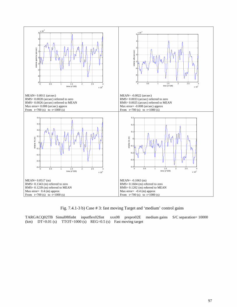
97

MEAN= 0.0011 (arcsec)RMS= 0.0028 (arcsec) referred to zeroRMS= 0.0026 (arcsec) referred to MEANMax error= 0.008 (arcsec) approxFrom t=700 (s) to t=1000 (s)

MEAN= -0.0022 (arcsec)RMS= 0.0033 (arcsec) referred to zeroRMS= 0.0025 (arcsec) referred to MEANMax error= -0.008 (arcsec) approxFrom t=700 (s) to t=1000 (s)

MEAN= 0.0517 (m)RMS= 0.1343 (m) referred to zeroRMS= 0.1239 (m) referred to MEANMax error= 0.4 (m) approxFrom t=700 (s) to t=1000 (s)

MEAN= -0.1063 (m)RMS= 0.1604 (m) referred to zeroRMS= 0.1202 (m) referred to MEANMax error= -0.4 (m) approxFrom t=700 (s) to t=1000 (s)

Fig. 7.4.1-3 b) Case # 3: fast moving Target and ‘medium’ control gains

TARGACQ02TB Simul08finbt inputflex02fint xxx08 prepro02E medium gains S/C separation= 10000(km) DT=0.01 (s) TTOT=1000 (s) REG=0.5 (s) Fast moving target

0 0.5 1 1.5 2 2.5 3

x 104

-8

-6

-4

-2

0

2

4

6

8x 10

-3

rela

tive

gam

ma

(arc

sec)

time (s*100)

0 0.5 1 1.5 2 2.5 3

x 104

-8

-6

-4

-2

0

2

4

6x 10

-3

rela

tive

alfa

(ar

csec

)

time (s*100)

0 0.5 1 1.5 2 2.5 3

x 104

-0.4

-0.3

-0.2

-0.1

0

0.1

0.2

0.3

0.4

rela

tive

Xs (

m)

time (s*100)0 0.5 1 1.5 2 2.5 3

x 104

-0.4

-0.3

-0.2

-0.1

0

0.1

0.2

0.3

rela

tive

Zs (

m)

time (s*100)

98

RMS= 3.0508e-006 (arcsec) from 1-50 Hz RMS= 3.2542e-006 (arcsec) from 1-50 Hz

RMS= 1.4791e-004 (m) from 1-50 Hz RMS= 1.5777e-004 (m) from 1-50 Hz

Fig. 7.4.1-3 c) Case # 3: fast moving Target and ‘medium’ control gains

TARGACQ02TC Simul08finbt inputflex02fint xxx08 prepro02E medium gains S/C separation= 10000(km) DT=0.01 (s) TTOT=1000 (s) REG=0.5 (s) Fast moving target

0 100 200 300 400 500 600 700 800 900 10000

0.1

0.2

0.3

0.4

0.5

0.6

0.7

0.8

0.9

1x 10

-6

rela

tive

gam

ma

fft (

arcs

ec)

rms

freq (Hz) shown range 1-10 Hz 0 100 200 300 400 500 600 700 800 900 10000

0.2

0.4

0.6

0.8

1

1.2x 10

-6

rela

tive

alfa

fft

(arc

sec)

rm

s

freq (Hz) shown range 1-10 Hz

0 100 200 300 400 500 600 700 800 900 10000

0.5

1

1.5

2

2.5

3

3.5

4

4.5x 10

-5

rela

tive

Xs ff

t (m

) rm

s

freq (Hz) shown range 1-10 Hz 0 100 200 300 400 500 600 700 800 900 10000

2

4

6x 10

-5

rela

tive

Zs ff

t (m

) rm

s

freq (Hz) shown range 1-10 Hz

99

MEAN POWER =11.4924 (W)

Fig. 7.4.1-3 d) Case # 3: fast moving target and ‘medium’ control gains

TARGACQ02TD Simul08finbt inputflex02fint xxx08 prepro02E medium gains S/C separation= 10000(km) DT=0.01 (s) TTOT=1000 (s) REG=0.5 (s) Fast moving target

0 1 2 3 4 5 6 7 8 9 10

x 104

0

1

2

3

4

5

6

7

8x 10

-7

fuel

cum

ulat

ive

cons

umpt

ion

(kg)

time (s*100)

0 1 2 3 4 5 6 7 8 9 10

x 104

0

10

20

30

40

50

60

70

80

90

pow

er c

onsu

mpt

ion

(W)

inpu

t to

thr

uste

rs e

lect

roni

cs

time (s*100)

0 1 2 3 4 5 6 7 8 9 10

x 104

0

2000

4000

6000

8000

10000

12000

ener

gy c

onsu

mpt

ion

(J)

inpu

t to

thr

uste

rs e

lect

roni

cs

time (s*100)

100

Case # 4: fast moving target with perturbed motion and P S/C controlled by KF with ‘low’ control gains

This case refers to the following situation:- the target spacecraft is in position free drift with high initial speeds conditions and with the X and Z

positions artificially perturbed stepwise; it is assumed in attitude control mode with respect to the targetnominal alignment frame (xenon thrusters and high resolution ST);

- the pointing spacecraft is in position free drift mode with high initial attitude errors; it is in relative totarget attitude mode guided by the information from the interferometric relative attitude sensor and FEEPthrusters integrated in a KF;

- the gains of the regulator are classified as ‘low’ since they allow initial a pronounced overshoot;- general features:

Total simulation time =1000(s);Measurement and regulator frequency = 2 Hz;Dynamic time step = 0.01 (s)

The achieved results are reported in fig. 7.4.1-4 a) to d) with KF not extended (and no perturbations in thesystem dynamic matrix).In fig. 7.4.1-4 e) the case is repeated with strong perturbations in the dynamic matrix (50% simulated error inyaw stiffness and pitch stiffness) and the KF extended to 40 states. The following comments apply:

- fig. 7.4.1-4 a) provides an overview of performances from T=0 (s) It is noted the initial overshot and afull settlement time of approximately 150 (s); the settlement time of the KF is in the order of 10 (s) for acovariance reduction from 100% to 20%;

- fig 7.4.1-4 b) provides the relative performances in time domain from T=700 (s) to T=1000 (s) withsome statistical information and drift position of target S/C (from T=0 s to T=1000 s). Overall pointingaccuracy is in the order of (per axis):

relative attitude error (rms) < 0.0027 arcsecrelative attitude error (max observed) < -0.0045 (arcsec)position on target error (rms)< 0.13 (m)position on target error (max observed) < -0.22 (m)

The target spacecraft position drift appears approximately 300 (m) which is due to the simulatedinitial high speed. Such drift is similar to the one expected in actual three hours mission;

- fig. 7.4.1-4 c) provides an overview of the performances in frequency domain (for f >1 Hz) as resultfrom data evaluation from T=900 (s) to T=1000 (s).Concerning the Target S/C the jitters in attitudes and displacements are reported from case#1:

target S/C attitude jitter (rms) < 8.3*1E-5*10= 8.3*1E-4 (arcsec) which induce a sensordisplacement in the order of 4.2*1E-8 (m) for a Target CM to Target sensor distance of 10(m);target S/C position jitter (rms)< 1.1*1E-12*10= 1.1*1E-11 (m)

Such target S/C behaviour still do not significantly affect the relative pointing performances at thetarget sensor plane which are controlled basically by the attitude related performances of the pointingspacecraft (which are reported in the figure); per axis they are:

jitter at target sensor plane (rms) (in terms of attitudes)< 1.6*1E-8 (arcsec)jitter at target sensor plane (rms) (in terms of displacements)<8*1E-7 (m)= 0.8 (µm)

It is noted the very strong reduction (factor 50-100) with respect to the case with no KF.

101

- fig 7.4.1-4 d) reports the total fuel consumption for this 1000 (s) mission. Also shown are the electricpower and energy at thrusters electronics input. It is noted a reduction of fuel consumption with respectto case #1 by a factor of approximately 10 (caused by low noise on the filtered state vector used for thecontrol). Assuming this type of control continuously active for two years the total amount of fuelconsumption (e.g. indium or cesium) would be 0.005 (kg).Concerning power and energy the sockets for the electronics are to be added.

- fig 7.4.1-4 e) reports the relative angles (gamma and alfa) showing that the system is stable and nodegradations appear due to the strong inaccuracies injected in the dynamic matrix.

102

Fig. 7.4.1-4 a) Case#4: Fast moving target with perturbed motion (P S/C control by KF and ‘low’ controlgains)

KFF5TA Simulkfbfin4t inputkfb01ft prepro02E low gains KF (with integrator and full memory) S/Cseparation = 10000 (km) DT=0.01 (s) TTOT=1000 (s) REG=0.5 (s) Fast moving targetDeltaXT=32 (m) Delta ZT=64 (m) @ T=250 (s)

0 1 2 3 4 5 6 7 8 9 10

x 104

-2

-1.5

-1

-0.5

0

0.5

1re

lativ

e ga

mm

a (a

rcse

c)

time (s*100) 0 1 2 3 4 5 6 7 8 9 10

x 104

-1.5

-1

-0.5

0

0.5

1

1.5

2

rela

tive

alfa

(ar

csec

)

time (s*100)

0 1 2 3 4 5 6 7 8 9 10

x 104

-100

-50

0

50

rela

tive

Xs (

m)

time (s*100)0 1 2 3 4 5 6 7 8 9 10

x 104

-80

-60

-40

-20

0

20

40

60

80

100

rela

tive

Zs (

m)

time (s*100)

0 200 400 600 800 1000 1200 1400 1600 1800 2000-2

-1.5

-1

-0.5

0

0.5

1

best

(K

F)r

elat

ive

gam

ma

(arc

sec)

time (s*2)0 200 400 600 800 1000 1200 1400 1600 1800 2000

-1.5

-1

-0.5

0

0.5

1

1.5

2

2.5

best

(K

F)

rela

tive

alfa

(ar

csec

)

time (s*2)

103

MEAN=0.0024 (arcsec)RMS= 0.0024 (arcsec) referred to zeroRMS= 4.3956e-004 (arcsec) referred to meanMax error= 0.0035 (arcsec) approxFrom T=700(s) to T=1000(s)

MEAN= -0.0024 (arcsec)RMS= 0.0027 (arcsec) referred to zeroRMS= 0.0011 (arcsec) referred to meanMax error= -0.0045 (arcsec) approxFrom T=700(s) to T=1000(s)

MEAN= 0.1147 (m)RMS= 0.1166 (m) referred to zeroRMS= 0.0213 (m) referred to meanMax error= 0.16 (m) approxFrom T=700(s) to T=1000(s)

MEAN= -0.1179 (m)RMS= 0.1286 (m) referred to zeroRMS= 0.0513 (m) referred to meanMax error= -0.22 (m) approxFrom T=700(s) to T=1000(s) curve

From T=0(s) to T=1000(s) From T=0(s) to T=1000(s)

Fig. 7.4.1-4 b) Case#4: Fast moving target with perturbed motion (P S/C control by KF and ‘low’ controlgains)

KFF5TB Simulkfbfin4t inputkfb01ft prepro02E low gains KF (with integrator and full memory) S/Cseparation = 10000 (km) DT=0.01 (s) TTOT=1000 (s) REG=0.5 (s) Fast moving targetDeltaXT=32 (m) Delta ZT=64 (m) @ T=250 (s)

0 0.5 1 1.5 2 2.5 3

x 104

1

1.5

2

2.5

3

3.5x 10

-3

rela

tive

gam

ma

(arc

sec)

time (s*100)

0 0.5 1 1.5 2 2.5 3

x 104

-4.5

-4

-3.5

-3

-2.5

-2

-1.5

-1

-0.5

0x 10

-3

rela

tive

alfa

(ar

csec

)

time (s*100)

0 0.5 1 1.5 2 2.5 3

x 104

0.06

0.08

0.1

0.12

0.14

0.16

0.18

rela

tive

Xs (

m)

time (s*100)0 0.5 1 1.5 2 2.5 3

x 104

-0.25

-0.2

-0.15

-0.1

-0.05

0

rela

tive

Zs (

m)

time (s*100)

0 1 2 3 4 5 6 7 8 9 10

x 104

0

50

100

150

200

250

300

350

400

X ta

rget

(m

)

time (s*100)0 1 2 3 4 5 6 7 8 9 10

x 104

0

50

100

150

200

250

300

350

400

Z ta

rget

(m

)

time (s*100)

104

RMS= 1.3433e-008 (arcsec) from 1 to 50 Hz RMS= 1.5360e-008 (arcsec) from 1 to 50 Hz

RMS= 6.5126e-007 (m) from 1 to 50 Hz RMS= 7.4467e-007 (m) from 1 to 50 Hz

Fig. 7.4.1-4 c) Case#4: Fast moving target with perturbed motion (P S/C control by KF and ‘low’ controlgains)

KFF5TC Simulkfbfin4t inputkfb01ft prepro02E low gains KF (with integrator and full memory) S/Cseparation = 10000 (km) DT=0.01 (s) TTOT=1000 (s) REG=0.5 (s) Fast moving targetDeltaXT=32 (m) Delta ZT=64 (m) @ T=250 (s)

0 100 200 300 400 500 600 700 800 900 10000

0.5

1

1.5

2

2.5

3

3.5

4x 10

-9

rela

tive

gam

ma

fft (

arcs

ec)

rms

freq (Hz) shown range 1-10 Hz

0 100 200 300 400 500 600 700 800 900 10000

1

2

3

4

5

6x 10

-9

rela

tive

alfa

fft

(arc

sec)

rm

s

freq (Hz) shown range 1-10 Hz

0 100 200 300 400 500 600 700 800 900 10000

0.2

0.4

0.6

0.8

1

1.2

1.4

1.6

1.8x 10

-7

rela

tive

Xs ff

t (m

) rm

s

freq (Hz) shown range 1-10 Hz0 100 200 300 400 500 600 700 800 900 1000

0

0.5

1

1.5

2

2.5

3x 10

-7

rela

tive

Zs ff

t (m

) rm

s

freq (Hz) shown range 1-10 Hz

105

Note: socket power consumption to be added to above power

Note: socket energy consumption rate to be added to above energy

Fig. 7.4.1-4 d) Case#4: Fast moving target with perturbed motion (P S/C control by KF and ‘low’ controlgains)

KFF5TD Simulkfbfin4t inputkfb01ft prepro02E low gains KF (with integrator and full memory) S/Cseparation = 10000 (km) DT=0.01 (s) TTOT=1000 (s) REG=0.5 (s) Fast moving targetDeltaXT=32 (m) Delta ZT=64 (m) @ T=250 (s)

0 1 2 3 4 5 6 7 8 9 10

x 104

0

1

2

3

4

5

6

7x 10

-8

fuel

cum

ulat

ive

cons

umpt

ion

(kg)

time (s*100)

0 1 2 3 4 5 6 7 8 9 10

x 104

0

10

20

30

40

50

60

70

pow

er c

onsu

mpt

ion

(W)

inpu

t to

thr

uste

rs e

lect

roni

cs

time (s*100)

0 1 2 3 4 5 6 7 8 9 10

x 104

0

100

200

300

400

500

600

700

800

900

1000

ener

gy c

onsu

mpt

ion

(J)

inpu

t to

thr

uste

rs e

lect

roni

cs

time (s*100)

106

0 1 2 3 4 5 6 7 8 9 10

x 104

-2

-1.5

-1

-0.5

0

0.5

1re

lativ

e ga

mm

a (a

rcse

c)

time (s*100)0 1 2 3 4 5 6 7 8 9 10

x 104

-1.5

-1

-0.5

0

0.5

1

1.5

2

rela

tive

alfa

(ar

csec

)

time (s*100)

0 0.5 1 1.5 2 2.5 3

x 104

1.8

2

2.2

2.4

2.6

2.8

3

3.2

3.4

3.6x 10

-3

rela

tive

gam

ma

(arc

sec)

time (s*100)

MEAN= 0.0028 (arcsec)RMS= 0.0028 (arcsec) referred to zeroRMS= 3.7918e-004 (arcsec) referred to meanMax error= 0.0036 (arcsec approx.From T=700 (s) to T=1000 (s)

0 0.5 1 1.5 2 2.5 3

x 104

-4

-3.5

-3

-2.5

-2

-1.5

-1

-0.5

0

0.5x 10

-3

rela

tive

alfa

(ar

csec

)

time (s*100)

MEAN= -0.0022 (arcsec)RMS= 0.0024 (arcsec) referred to zeroRMS= 0.0010 (arcsec) referred to meanMax error= -0.0039 (arcsec approx.From T=700 (s) to T=1000 (s)

0 100 200 300 400 500 600 700 800 900 10000

0.5

1

1.5

2

2.5

3

3.5

4x 10

-9

rela

tive

gam

ma

fft (

arcs

ec)

rms

freq (Hz) shown range 1-10 Hz

RMS= 1.3649e-008 (arcsec) from 1 to 50 Hz

0 100 200 300 400 500 600 700 800 900 10000

1

2

3

4

5

6x 10

-9

rela

tive

alfa

fft

(arc

sec)

rm

s

freq (Hz) shown range 1-10 Hz

RMS= 1.7090e-008 (arcsec) from 1 to 50 Hz

Fig. 7.4.1-4 e) Case#4: Fast moving target with perturbed motion (P S/C control by KF extended and ‘low’control gains)

EXTENCIA Simulkfext2 inputext2 KANGX*1.5 KANGZ*1.5 with integrator S/C separation =10000 km DT=0.01 (s)TTOT = 10000 (s) REG = 0.5 (s) DeltaXT=32 (m) Delta ZT=64 (m) @ T=250 (s)

107

Case # 5: fast moving target with perturbed motion and P S/C controlled by KF with ‘high‘ gains determinedwith optimum techniques

This case refers to the following situation:- the target spacecraft is in position free drift with high initial speeds conditions and with the X and Z

positions artificially perturbed stepwise; it is assumed in attitude control mode with respect to the targetnominal alignment frame (xenon thrusters and high resolution ST);

- the pointing spacecraft is in position free drift mode with high initial attitude errors; it is in relative totarget attitude mode guided by the information from the interferometric relative attitude sensor and FEEPthrusters integrated in a KF;

- the regulator gains (high) have been selected with deterministic optimum tecqniques and in the specificcase reported compromising pointing errors and fuel consumption in a ratio 9:1 in the weighingfunctional:

Q(1,1)=Q(3,3)=16000 Q(2,2)=4.8 R(1,1)=R(3,3)=0.8 R(2,2)=0.08

with the overall aim to have a fast responding system and accurate.

- general features:Total simulation time =1000(s);Measurement and regulator frequency = 2 Hz;Dynamic time step = 0.01 (s)

The achieved results are reported in fig. 7.4.1-5 a) to c) and the following comments apply:

- fig. 7.4.1-5 a) provides an overview of performances from T=0 (s) It is noted the initial overshot reducedto 50% of the one using ‘intermediate gains’ and a full settlement time of approximately 30 (s) followedby a residual smooth converging phase to the commanded relative attitudes;

- fig 7.4.1-5 b) provides the relative performances in time domain from T=700 (s) to T=1000 (s) withsome statistical information and the result of a 2000 (s) simulation aiming at explore the overall stabilityassociated to the modified KF. Overall pointing accuracy is in the order of (per axis):

relative attitude error (rms) < 0.0028 arcsecrelative attitude error (max observed) < -0.0045 (arcsec)position on target error (rms)< 0.14 (m)position on target error (max observed) < -0.22 (m)

- fig. 7.4.1-5 c) provides an overview of the performances in frequency domain (for f >1 Hz) as resultfrom data evaluation from T=900 (s) to T=1000 (s).The relative pointing performances at the target sensor plane are controlled basically by the attituderelated performances of the pointing spacecraft (which are reported in the figure); per axis they are:

jitter at target sensor plane (rms) (in terms of attitudes)< 1.3*1E-7 (arcsec)jitter at target sensor plane (rms) (in terms of displacements)<6.2*1E-6 (m)= 6.2 (µm)

It is noted the increased bandwidth is achieved at the expenses of jitter performances above 1Hz.

108

0 200 400 600 800 1000 1200 1400 1600 1800 2000-1.5

-1

-0.5

0

0.5

1

1.5

2

2.5

best

(K

F)

rela

tive

alfa

(ar

csec

)

time (s*2)

Fig. 7.4.1-5 a) Case # 5: fast moving target with perturbed motion and P S/C controlled by KF with ‘highoptimum‘ gains

KFF6TA Simulkfbfin4t inputkfb02ft prepro02E ‘optimum’ gains KF (with integrator and full memory)S/C separation= 10000 (km) DT=0.01 (s) TTOT=1000 (s) REG=0.5 (s) Fast moving targetDeltaXT=32 (m) Delta ZT=64 (m) @ T=250 (s)

0 1 2 3 4 5 6 7 8 9 10

x 104

-1.8

-1.6

-1.4

-1.2

-1

-0.8

-0.6

-0.4

-0.2

0

0.2

rela

tive

gam

ma

(arc

sec)

time (s*100)0 1 2 3 4 5 6 7 8 9 10

x 104

-1.5

-1

-0.5

0

0.5

1

1.5

2

rela

tive

alfa

(ar

csec

)

time (s*100)

0 1 2 3 4 5 6 7 8 9 10

x 104

-90

-80

-70

-60

-50

-40

-30

-20

-10

0

10

rela

tive

Xs (

m)

time (s*100)0 1 2 3 4 5 6 7 8 9 10

x 104

-80

-60

-40

-20

0

20

40

60

80

100

rela

tive

Zs (

m)

time (s*100)

0 200 400 600 800 1000 1200 1400 1600 1800 2000-1.8

-1.6

-1.4

-1.2

-1

-0.8

-0.6

-0.4

-0.2

0

0.2

best

(K

F)

rela

tive

gam

ma

(arc

sec)

time (s*2)

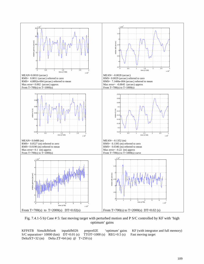
109

MEAN=0.0010 (arcsec)RMS= 0.0011 (arcsec) referred to zeroRMS= 4.0892e-004 (arcsec) referred to meanMax error= 0.002 (arcsec) approxFrom T=700(s) to T=1000(s)

MEAN= -0.0028 (arcsec)RMS= 0.0029 (arcsec) referred to zeroRMS= 7.1406e-004 (arcsec) referred to meanMax error= -0.0045 (arcsec) approxFrom T=700(s) to T=1000(s)

MEAN= 0.0488 (m)RMS= 0.0527 (m) referred to zeroRMS= 0.0198 (m) referred to meanMax error= 0.1 (m) approxFrom T=700(s) to T=1000(s)

MEAN= -0.1352 (m)RMS= 0.1395 (m) referred to zeroRMS= 0.0346 (m) referred to meanMax error= -0.22 (m) approxFrom T=700(s) to T=1000(s) curve

From T=700(s) to T=2000(s) DT=0.02(s) From T=700(s) to T=2000(s) DT=0.02 (s)

Fig. 7.4.1-5 b) Case # 5: fast moving target with perturbed motion and P S/C controlled by KF with ‘highoptimum‘ gains

KFF6TB Simulkfbfin4t inputkfb02ft prepro02E ‘optimum’ gains KF (with integrator and full memory)S/C separation= 10000 (km) DT=0.01 (s) TTOT=1000 (s) REG=0.5 (s) Fast moving targetDeltaXT=32 (m) Delta ZT=64 (m) @ T=250 (s)

0 0.5 1 1.5 2 2.5 3

x 104

-5

0

5

10

15

20x 10

-4

rela

tive

gam

ma

(arc

sec)

time (s*100)

0 0.5 1 1.5 2 2.5 3

x 104

-4.5

-4

-3.5

-3

-2.5

-2

-1.5

-1x 10

-3

rela

tive

alfa

(ar

csec

)

time (s*100)

0 0.5 1 1.5 2 2.5 3

x 104

-0.02

0

0.02

0.04

0.06

0.08

0.1

rela

tive

Xs (

m)

time (s*100)0 0.5 1 1.5 2 2.5 3

x 104

-0.22

-0.2

-0.18

-0.16

-0.14

-0.12

-0.1

-0.08

-0.06

-0.04

rela

tive

Zs (

m)

time (s*100)

0 1 2 3 4 5 6 7

x 104

-1

0

1

2

3

4

5x 10

-3

rela

tive

gam

ma

(arc

sec)

time (s*50)

0 1 2 3 4 5 6 7

x 104

-4

-3.5

-3

-2.5

-2

-1.5

-1x 10

-3

rela

tive

alfa

(ar

csec

)

time (s*50)

110

RMS= 1.2675e-007 (arcsec) from 1 to 50 Hz RMS= 1.1035e-007 (arcsec) from 1 to 50 Hz

RMS= 6.1449e-006 (m) from 1 to 50 Hz RMS= 5.3500e-006 (m) from 1 to 50 Hz

Fig. 7.4.1-5 c) Case # 5: fast moving target with perturbed motion and P S/C controlled by KF with ‘highoptimum‘ gains

KFF6TC Simulkfbfin4t inputkfb02ft prepro02E ‘optimum’ gains KF (with integrator and full memory)S/C separation= 10000 (km) DT=0.01 (s) TTOT=1000 (s) REG=0.5 (s) Fast moving targetDeltaXT=32 (m) Delta ZT=64 (m) @ T=250 (s)

0 100 200 300 400 500 600 700 800 900 10000

0.5

1

1.5

2

2.5

3

3.5x 10

-8

rela

tive

gam

ma

fft (

arcs

ec)

rms

freq (Hz) shown range 1-10 Hz

0 100 200 300 400 500 600 700 800 900 10000

0.5

1

1.5

2

2.5

3

3.5

4x 10

-8

rela

tive

alfa

fft

(arc

sec)

rm

s

freq (Hz) shown range 1-10 Hz

0 100 200 300 400 500 600 700 800 900 10000

0.2

0.4

0.6

0.8

1

1.2

1.4

1.6

1.8x 10

-6

rela

tive

Xs ff

t (m

) rm

s

freq (Hz) shown range 1-10 Hz

0 100 200 300 400 500 600 700 800 900 10000

0.2

0.4

0.6

0.8

1

1.2

1.4

1.6

1.8

2x 10

-6

rela

tive

Zs ff

t (m

) rm

s

freq (Hz) shown range 1-10 Hz

111

7.4.2 Scientific phase

In this phase the scientific part of the mission is envisaged. The scientific phase is characterised by thefollowing basic features:

- its duration can be set to approximately three hours (then it repeats);- during this period neither the Target S/C nor the Pointing S/C are controlled in position: they can

drift freely under the influence of the external perturbations up to few hundreds of meters;- the scientific phase can be considered formed by two repeating sub-phases: the scientific

measurement sub-phase and the target re-acquisition and attitude recovery sub-phase;- during the scientific measurement sub-phase both the Target S/C and the Pointing S/C are freely

drifting also in attitudes so to reduce the jitter to an absolute minimum. In this period the line of sightof the optical platform of the Pointing S/C hits the wide sensor at the Target S/C and slowly drifts onit until exit (this sub phase can last 40-60 seconds) and the true scientific measurements performed;

- once the exit from the wide sensor has happened the attitude recovery sub phase take place (withinthe next e.g. 200 seconds):

the Pointing S/C recover its line of sight onto the target wide sensor via relative attitudecontrol (using the high performing interferometric relative sensor) to accuracies <0.01(arcsec);

the Target S/C recovers its coarse attitude with respect to the local alignment frame aimingat the Pointing S/C with moderate accuracies (e.g. < 5 arcsec). The attitude of the TargetS/C can be controlled by utilising absolute attitude informations provided by the on boardhigh accuracy star tracker. The pointing coordinates can be computed with respect to thelocal nominal alignment frame knowing the positions of the Target and Pointing S/C withrespect to the local frames within several tens of meters;

- when the spacecrafts have abandoned the nominal position by more than some hundereds ofmeters the scientific phase is suspended and the position of the spacecrafts recovered (asillustrated in the next paragraph)

Four study cases (out of the whole cases evaluated) are hereafter reported:

- Case # 6: scientific phase with fast moving target;- Case # 7: scientific phase with fast moving target and perturbation plus increased radiation pressure

torque imbalance- Case # 8: measurement sub phase;- Case # 9: measurement sub phase with increased radiation pressure noise and radiation pressure torque

imbalance.

These cases are here below presented and commented.

Case # 6: scientific phase with fast moving target

This case provides an overall view of the mission showing the overall behaviour of some importantparameters for an overall simulation time of 700 (s). The results are reported in fig. 7.4.2-1 from a) to c) andthe following comments apply:

- fig. 7.4.2-1a) provides an overview of performances in terms of relative attitudes and centering on thetarget sensor plane, Are clearly visible the phases with attitude control active (target acquisition) and freedrift (measurment sub phase). Each free drift sub phase, defined as the time necessary for the line ofsight to drift 12 (m) at the target sensor plane, lasts approximately 60 (s) as also appears from fig. 7.4.2-1c). Also shown are the profile of the X coordinate of the Target S/C as it evolves and the pitch derivativeangle of the pointing S/C (referred to the local alignment frame) showing the rate necessary for tracking.

112

- fig 7.4.2-1 b) provides a drawing showing the relative motion of the line of sight at the target sensorplane and the derivatives of the relative attitude angles. It appears that at the end of each target trackingphase a relative speed of less than 0.001-0.002 (arcsec/s) is achieved. The target tracking phase isconsidered achieved based on distance criteria from the centre target and stabilisation time;

- fig. 7.4.2-1 c) provides the profiles of the commanded torques (from which clearly appears the driftingsub phase) and the fuel, power, energy profiles necessary to achieve the shown mission. Forces are notshown since they are null. Assuming to perform the scientific phase with a duty cycle 1:2 with respect tothe recovery phase then, for a 1.5 year orbit operation, a total of 7 (grams) of fuel would be necessary, inthe evaluated case indium or cesium.

Case # 7: scientific phase with fast moving target and perturbation plus increased radiation pressure torqueimbalance

With respect to Case # 6 an increase of the torque imbalance for the radiation pressure by a factor of three isconsidered (which corresponds for the specific case to approximately 15% average non homogeneity overtwo halves of S/C). Furthermore a sudden position perturbation to the Target S/C is superimposed. In thiscase a line of sight drift of 20 (m) has been considered and the resulting free drift time appears approximately43 (s); the considered drift distance is still fully compatible with sensor at target size in the range of 30-40 mstill in the technology range. The results are reported in fig. 7.4.2-2 from a) to c) and the following commentsof the same type as per Case #6 apply. Furthermore the following are noted:

- the perturbation has been applied at T= 340 (s) during a drifting sub phase;- this perturbation cause the line of sight to relatively drift to more tha 20 (m) and this re activate the

attitude control;- the effect of the perturbation is also clearly visible on the plane of the sensor at target S/C.

113

Fig. 7.4.2-1a) Case # 6: scientific phase with fast moving target

ONOFF1TA Simul06bt inputmission06c01ft dataeval feep01 FFEP interferometer fast moving targetDT=0.01(s) TTOT=700(s) REG=0.5(s) RINF=0.5(m) RSUP=12(m) ‘low gains’

0 1 2 3 4 5 6 7

x 104

-0.4

-0.3

-0.2

-0.1

0

0.1

0.2

0.3re

lativ

e ga

mm

a (a

rcse

c)

time (s*100)0 1 2 3 4 5 6 7

x 104

-0.2

-0.1

0

0.1

0.2

0.3

0.4

0.5

rela

tive

alfa

(ar

csec

)

time (s*100)

0 1 2 3 4 5 6 7

x 104

-20

-15

-10

-5

0

5

10

15

rela

tive

Xs (

m)

time (s*100)0 1 2 3 4 5 6 7

x 104

-10

-5

0

5

10

15

20

rela

tive

Zs (

m)

time (s*100)

0 1 2 3 4 5 6 7

x 104

0

50

100

150

200

250

X ta

rget

(m

)

time (s*100)

0 1 2 3 4 5 6 7

x 104

-0.015

-0.01

-0.005

0

0.005

0.01

0.015

0.02

0.025

gam

mad

ot o

pt (

arcs

ec/s

)

time (s*100)

114

Fig. 7.4.2-1b) Case # 6: scientific phase with fast moving target

ONOFF1TB Simul06bt inputmission06c01ft dataeval feep01 FFEP interferometer fast moving targetDT=0.01(s) TTOT=700(s) REG=0.5(s) RINF=0.5(m) RSUP=12(m) ‘low gains’

0 200 400 600 800 1000 1200 1400-0.02

-0.015

-0.01

-0.005

0

0.005

0.01

0.015

0.02

rela

tive

gam

ma

spee

d (a

rcse

c/s)

time (s*2)0 200 400 600 800 1000 1200 1400

-0.03

-0.025

-0.02

-0.015

-0.01

-0.005

0

0.005

0.01

rela

tive

alfa

spe

ed (

arcs

ec/s

)

time (s*2)

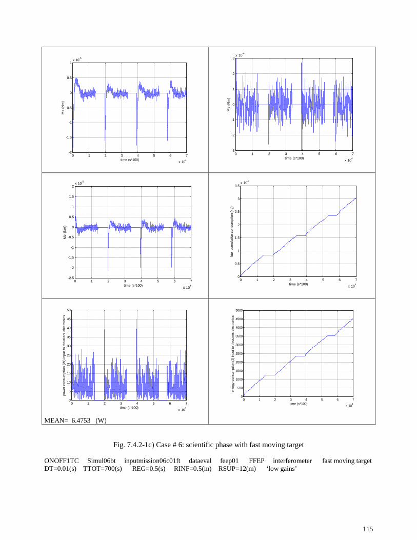
115

MEAN= 6.4753 (W)

Fig. 7.4.2-1c) Case # 6: scientific phase with fast moving target

ONOFF1TC Simul06bt inputmission06c01ft dataeval feep01 FFEP interferometer fast moving targetDT=0.01(s) TTOT=700(s) REG=0.5(s) RINF=0.5(m) RSUP=12(m) ‘low gains’

0 1 2 3 4 5 6 7

x 104

-2

-1.5

-1

-0.5

0

0.5

1x 10

-5

Mx

(Nm

)

time (s*100)

0 1 2 3 4 5 6 7

x 104

-3

-2

-1

0

1

2

3x 10

-4

My

(Nm

)

time (s*100)

0 1 2 3 4 5 6 7

x 104

-2.5

-2

-1.5

-1

-0.5

0

0.5

1

1.5

2x 10

-5

Mz

(Nm

)

time (s*100)

0 1 2 3 4 5 6 7

x 104

0

0.5

1

1.5

2

2.5

3

3.5x 10

-7

fuel

cum

ulat

ive

cons

umpt

ion

(kg)

time (s*100)

0 1 2 3 4 5 6 7

x 104

0

5

10

15

20

25

30

35

40

45

50

pow

er c

onsu

mpt

ion

(W)

inpu

t to

thr

uste

rs e

lect

roni

cs

time (s*100)

0 1 2 3 4 5 6 7

x 104

0

500

1000

1500

2000

2500

3000

3500

4000

4500

5000

ener

gy c

onsu

mpt

ion

(J)

inpu

t to

thr

uste

rs e

lect

roni

cs

time (s*100)

116

Fig. 7.4.2-2 a ) Case # 7: scientific phase with fast moving target and perturbation plus increasedradiation pressure torque imbalance

ONOFF2TA Simul06bt inputmission06c02ft dataeval feep01 FFEP interferometer fast moving targetwith perturbation DT=0.01(s) TTOT=700(s) REG=0.5(s) RINF=0.5(m) RSUP=12(m) ‘low gains’DELTAXT=16(m) DELTAZT=32 (m) @T= 340 (s)

0 1 2 3 4 5 6 7

x 104

-0.4

-0.3

-0.2

-0.1

0

0.1

0.2

0.3

0.4re

lativ

e ga

mm

a (a

rcse

c)

time (s*100) 0 1 2 3 4 5 6 7

x 104

-0.8

-0.6

-0.4

-0.2

0

0.2

0.4

0.6

rela

tive

alfa

(ar

csec

)

time (s*100)

0 1 2 3 4 5 6 7

x 104

-20

-15

-10

-5

0

5

10

15

20

rela

tive

Xs (

m)

time (s*100)0 1 2 3 4 5 6 7

x 104

-40

-30

-20

-10

0

10

20

rela

tive

Zs (

m)

time (s*100)

0 1 2 3 4 5 6 7

x 104

0

50

100

150

200

250

X ta

rget

(m

)

time (s*100)0 1 2 3 4 5 6 7

x 104

0

50

100

150

200

250

Z ta

rget

(m

)

time (s*100)

117

From t=0 (s) to t=300 (s)

Fig. 7.4.2-2 b ) Case # 7: scientific phase with fast moving target and perturbation plus increased radiationpressure torque imbalance

ONOFF2TB Simul06bt inputmission06c02ft dataeval feep01 FFEP interferometer fast moving targetwith perturbation DT=0.01(s) TTOT=700(s) REG=0.5(s) RINF=0.5(m) RSUP=12(m) ‘low gains’DELTAXT=16 (m) DELTAZT=32 (m) @T= 340 (s)

0 200 400 600 800 1000 1200 14000

5

10

15

20

25

30

35

cent

er t

arge

t tr

ue r

elat

ive

dist

ance

(m

)

time (s*2)0 100 200 300 400 500 600

-0.03

-0.025

-0.02

-0.015

-0.01

-0.005

0

0.005

0.01

0.015

0.02

rela

tive

gam

ma

spee

d (a

rcse

c/s)

time (s*2)

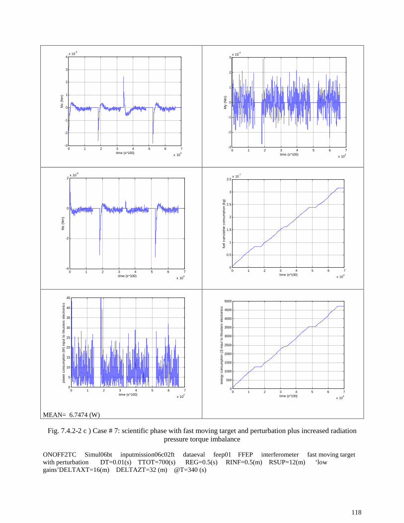
118

MEAN= 6.7474 (W)

Fig. 7.4.2-2 c ) Case # 7: scientific phase with fast moving target and perturbation plus increased radiationpressure torque imbalance

ONOFF2TC Simul06bt inputmission06c02ft dataeval feep01 FFEP interferometer fast moving targetwith perturbation DT=0.01(s) TTOT=700(s) REG=0.5(s) RINF=0.5(m) RSUP=12(m) ‘lowgains’DELTAXT=16(m) DELTAZT=32 (m) @T=340 (s)

0 1 2 3 4 5 6 7

x 104

-3

-2

-1

0

1

2

3

4x 10

-5

Mx

(Nm

)

time (s*100)0 1 2 3 4 5 6 7

x 104

-3

-2

-1

0

1

2

3x 10

-4

My

(Nm

)

time (s*100)

0 1 2 3 4 5 6 7

x 104

-4

-2

0

2x 10

-5

Mz

(Nm

)

time (s*100)

0 1 2 3 4 5 6 7

x 104

0

0.5

1

1.5

2

2.5

3

3.5x 10

-7

fuel

cum

ulat

ive

cons

umpt

ion

(kg)

time (s*100)

0 1 2 3 4 5 6 7

x 104

0

5

10

15

20

25

30

35

40

45

pow

er c

onsu

mpt

ion

(W)

inpu

t to

thr

uste

rs e

lect

roni

cs

time (s*100)0 1 2 3 4 5 6 7

x 104

0

500

1000

1500

2000

2500

3000

3500

4000

4500

5000

ener

gy c

onsu

mpt

ion

(J)

inpu

t to

thr

uste

rs e

lect

roni

cs

time (s*100)

119

Case # 8: measurement sub phase

This case explores the relative pointing jitters during the true scientific part of the mission when thespacecrafts are in total drifting mode. The time duration for the measurement phase has been artificiallyextended with respect to the real ones (40-60 seconds) in order to allow a better frequency resolution for theanalysis.The results are reported in fig. 7.4.2-3 and the following comments apply:

- the jitter on relative line of sight pointing is basically caused by the jitter of the Pointing S/C relativeattitudes and the jitters in position appears negligible;

- the following performances are achievable (per axis):

jitter at target sensor plane (rms) (in terms of attitudes)< 1.1*1E-12 (arcsec)jitter at target sensor plane (rms) (in terms of displacements)<5.3*1E-11 (m)= 53 (pm)

In principle, if the sensor at the target S/C allows it, very accurate transversal measurments of the laser beamspot would be possible.

Case # 9: measurement sub phase with increased radiation pressure noise and radiation pressure torqueimbalance.

With respect to case # 8 the following modifications are done:• the torque imbalance for the radiation pressure is increased by a factor of of three (which

corresponds for the specific case to approximately 15% average non homogeneity over two halves ofS/C);

• the Power Spectra Density of the basic white noise of the solar radiation fluctuations has beenincreased by a factor of four.

The results are reported in fig. 7.4.2-4 and the following comments apply:

- the following performances are achievable (per axis):

jitter at target sensor plane (rms) (in terms of attitudes)< 6.5*1E-12 (arcsec)jitter at target sensor plane (rms) (in terms of displacements)<3.2*1E-10 (m)= 0.32 (nm)

- such performances, degrade by a factor of 6 with respect to the ones reported at Case # 8, arecompatible with the modified parameters (increase on RMS by 3*√4=6)

120

RMS= 1.0820e-012 (arcsec) from 1 to 50 Hz RMS= 9.3397e-013 (arcsec) from 1 to 50 Hz

RMS= 5.2454e-011 (m) from 1 to 50 Hz RMS= 4.5280e-011 (m) from 1 to 50 Hz

0 100 200 300 400 500 600 700 800 900 10000

1

2

3

4

5

6x 10

-17

X op

t fft

(m

) rm

s

freq (Hz) shown range 1-10 Hz

RMS= 2.2569e-016 (m) from 1 to 50 Hz

0 100 200 300 400 500 600 700 800 900 10000

1

2

3

4

5

6

7x 10

-17

Z op

t fft

(m

) rm

s

freq (Hz) shown range 1-10 Hz

RMS= 2.0022e-016 (m) from 1 to 50 Hz

Fig. 7.4.2-3Case # 8: measurement sub phase

SCIENF01A/D Simul08finb inputflexsci01fin xxx08 prepro02E free drift S/C separation= 10000 (km)DT=0.01 (s) TTOT=1000 (s) REG=N.A. (s) Rad. press. torque unb=5% Rad. press PSD=10

0 100 200 300 400 500 600 700 800 900 10000

0.2

0.4

0.6

0.8

1

1.2

1.4

1.6

1.8

2x 10

-11

rela

tive

Xs ff

t (m

) rm

s

freq (Hz) shown range 1-10 Hz0 100 200 300 400 500 600 700 800 900 1000

0

0.2

0.4

0.6

0.8

1

1.2

1.4x 10

-11

rela

tive

Zs ff

t (m

) rm

s

freq (Hz) shown range 1-10 Hz

0 100 200 300 400 500 600 700 800 900 10000

0.5

1

1.5

2

2.5

3

3.5

4x 10

-13

rela

tive

gam

ma

fft (

arcs

ec)

rms

freq (Hz) shown range 1-10 Hz0 100 200 300 400 500 600 700 800 900 1000

0

0.5

1

1.5

2

2.5

3

3.5x 10

-13

rela

tive

alfa

fft

(arc

sec)

rm

s

freq (Hz) shown range 1-10 Hz

121

RMS= 6.4917e-012 (arcsec) from 1 to 50 Hz RMS= 5.6284e-012 (arcsec) from 1 to 50 Hz

RMS= 3.1473e-010 (m) from 1 to 50 Hz RMS= 2.7287e-010 (m) from 1 to 50 Hz

Fig. 7.4.2-4 Case # 9: measurement sub phase with increased radiation pressure noise and radiation pressuretorque imbalance.

SCIENF03B Simul08finb inputflexsci03finbis(except where noted) xxx08 prepro02E free driftS/C separation= 10000 (km) DT=0.01 (s) TTOT=100 (s) REG=N.A. (s)Rad. press. torque unb=15% (three times Case 8) Rad. press PSD=40 (PSD four times Case 8)

0 100 200 300 400 500 600 700 800 900 10000

0.5

1

1.5

2

2.5x 10

-12

rela

tive

gam

ma

fft (

arcs

ec)

rms

freq (Hz) shown range 1-10 Hz

0 100 200 300 400 500 600 700 800 900 10000

0.2

0.4

0.6

0.8

1

1.2

1.4

1.6

1.8x 10

-12

rela

tive

alfa

fft

(arc

sec)

rm

s

freq (Hz) shown range 1-10 Hz

0 100 200 300 400 500 600 700 800 900 10000

0.2

0.4

0.6

0.8

1

1.2x 10

-10

rela

tive

Xs ff

t (m

) rm

s

freq (Hz) shown range 1-10 Hz0 100 200 300 400 500 600 700 800 900 1000

0

1

2

3

4

5

6

7

8

9x 10

-11

rela

tive

Zs ff

t (m

) rm

s

freq (Hz) shown range 1-10 Hz

122

7.4.3 Position Recovery phase

During this phase the recovery of the nominal allocated position is performed. As pointed out at paragraph7.3.2 the recovery command will be done by utilising a reference generated trajectory which can allow theexecution of a controlled recovery profile. The recovery can be performed in absolute mode by utilising highlevel thrusters (e.g. xenon based ) and high accuracy star trackers.A possible strategy is to perform the recovery at the end of each scientific phase (lasting approximately twoto three hours) and this will require at least a double amount of time to be completed by using xenonthrusters.During the scientific phase the position control is off and a position drift in the order of some hunderds ofmeters will grow. Starting from this, the recovery profile is generated.The manoeuvre can be performed with different level of performances depending on fidelity needed tofollow the generated profile. In the approach considered the position recovery can be performed in absolutecontrol and indeed there is no a specific need to follow the generated profile with great accuracy. During therecovery maneuver the electric power demand is ‘high’ and, as mentioned, specific solar panels need bedeployed to be then folded back and rigidised at the end of the recovery phase itself. One specific case isreported and hereafter discussed:

Case # 10: position recovery after scientific phase

In general the behaviour during recovery is time variant since it depends from the relative Earth-S/C-Moon-Sun positions. In the case shown a kind of worst case situation has been considered since the startingconditions has been assumed around the full alignment of the bodies involved. The results are shown in fig.7.4.3-1 a), b) c) and d) and the following remarks are noted:- the recovery starts from an initial position offset of about 330 (m) and initial speeds which would

accumulate from a previous Scientific phase lasting in the order of three hours;- the first step of the recovery manoeuvre (fig. 7.4.3-1 a and b) lasts about 8113 (s) and slow down the

S/C motion to zero speed while the position error would grow to about 600 (m); the second step (fig.7.4.3-1 c and d) lasts about 14006 (s) and would bring the S/C to its zero position with zero speedready to start a new scientific phase;

- the total fuel consumption for the recovery (in the assumed conditions) result approximately 0.021(kg) which would lead for a 1.5 years mission to approximately 30 (kg) of fuel (e,g, xenon);

- the electric power consumption present an average value of 920 (W) approximately with sustainedperiod of 1400 (W) which will pose due requirements on the Power and Distribution System.

While the time is evolving the perturbation effects from the Sun and Earth are continuously changing but wecan assume the case reported representative for the feasibility of the manoeuver. This case is run withoptimum gains and a reduction of noises on the x, y, z measurments certainly allowed by Kalman Filtering.To support the power demand during recovery phase it is necessary to foresee an extra solar panel surfacewith respect to the body mounted one. With reference to a power level of 1160 (W) (laying between theaverage value and the maximum value) then a surface area of 6 (m²) would be needed according to thefollowing assumptions:

- technology: triple junction- efficiency EOL (1.5 years)= 25%- efficiency optical coating= 0.9- average geometrical losses (only one angular compensation)= 0.9- surface filling= 0.9- power management= 0.9

123

0 0.5 1 1.5 2 2.5 3 3.5 4 4.5 5

x 105

300

350

400

450

500

550co

mm

ande

d X

opt

(m)

time (s*50)0 0.5 1 1.5 2 2.5 3 3.5 4 4.5 5

x 105

300

350

400

450

500

550

X op

t (m

)

time (s*50)

0 0.5 1 1.5 2 2.5 3 3.5 4 4.5 5

x 105

-190

-180

-170

-160

-150

-140

-130

-120

-110

-100

com

man

ded

Y o

pt (

m)

time (s*50) 0 0.5 1 1.5 2 2.5 3 3.5 4 4.5 5

x 105

-190

-180

-170

-160

-150

-140

-130

-120

-110

-100

Y o

pt (

m)

time (s*50)

0 0.5 1 1.5 2 2.5 3 3.5 4 4.5 5

x 105

100

110

120

130

140

150

160

170

180

com

man

ded

Z op

t (m

)

time (s*50)0 0.5 1 1.5 2 2.5 3 3.5 4 4.5 5

x 105

100

110

120

130

140

150

160

170

180

Z op

t (m

)

time (s*50)

Fig. 7.4.3-1 a) Case # 10: Position recovery after scientific phase (first step).

STASP05A Simul0sdin1 inputrecovery0sdin1 trajectory0speed2 DT=0.02 (s) TTOT=10000 (s)REG=0.5 (s) TRF= 3.2 TMAN= 8113 (s) Xo=300 (m) Yo=-100 (m) Zo=100 (m) Vxo=0.06 (m/s)Vyo=-0.02 (m/s) Vzo=0.02 (m/s)(Note: relative means w.r.t. a Target S/C in nominal orbital position-control performed in absolute mode via highaccuracy star tracker)

124

0 0.5 1 1.5 2 2.5 3 3.5 4 4.5 5

x 105

-0.02

-0.015

-0.01

-0.005

0

0.005

0.01

0.015

0.02F

x (N

)

time (s*50)

0 0.5 1 1.5 2 2.5 3 3.5 4 4.5 5

x 105

0

0.001

0.002

0.003

0.004

0.005

0.006

0.007

0.008

0.009

0.01

cum

ulat

ive

fuel

con

sum

ptio

n (k

g)

time (s*50)

FUEL (TMAN) = 0.00789 (kg)

MEAN (TMAN)= 9.18e+002 (W)

0 0.5 1 1.5 2 2.5 3 3.5 4 4.5 5

x 105

-1

0

1

2

3

4

5

erro

r X

opt

(m)

time (s*50)

Fig. 7.4.3-1 b) Case # 10: Position recovery after scientific phase (first step).

STASP05B Simul0sdin1 inputrecovery0sdin1 trajectory0speed2 DT=0.02 (s) TTOT=10000 (s)REG=0.5 (s) TRF= 3.2 TMAN= 8113 (s) Xo=300 (m) Yo=-100 (m) Zo=100 (m) Vxo=0.06 (m/s)Vyo=-0.02 (m/s) Vzo=0.02 (m/s)(Note: relative means w.r.t. a Target S/C in nominal orbital position-control performed in absolute mode via highaccuracy star tracker)

125

0 1 2 3 4 5 6 7 8

x 105

0

100

200

300

400

500

600co

mm

ande

d X

opt

(m)

time (s*50)0 1 2 3 4 5 6 7 8

x 105

-100

0

100

200

300

400

500

600

X op

t (m

)

time (s*50)

0 1 2 3 4 5 6 7 8

x 105

-200

-180

-160

-140

-120

-100

-80

-60

-40

-20

0

com

man

ded

Y o

pt (

m)

time (s*50) 0 1 2 3 4 5 6 7 8

x 105

-200

-150

-100

-50

0

50

Y o

pt (

m)

time (s*50)

0 1 2 3 4 5 6 7 8

x 105

0

20

40

60

80

100

120

140

160

180

200

com

man

ded

Z op

t (m

)

time (s*50) 0 1 2 3 4 5 6 7 8

x 105

0

20

40

60

80

100

120

140

160

180

200

Z op

t (m

)

time (s*50)

Fig. 7.4.3-1 c) Case # 10: Position recovery after scientific phase (second step).

RF5A Simul05terdin trajectory05sens (NTT=1/3 TRF=3) inputrf5 X0=545 (m) Y0=-182 (m) Z0=180 (m)VX0=0.001 (m/s) VY0=0.001 (m/s) VZ0= 0.001 (m/s) (optimum gains) TMAN= 14006 (s) DT=0.02 (s)TTOT= 14000 (s) REG=0.5 (s) TPREVM=8113 (s)

126

0 1 2 3 4 5 6 7 8

x 105

-0.02

-0.015

-0.01

-0.005

0

0.005

0.01

0.015

0.02

Fx

(N)

time (s*50)

0 1 2 3 4 5 6 7 8

x 105

0

0.005

0.01

0.015

cum

ulat

ive

fuel

con

sum

ptio

n (k

g)

time (s*50)

FUEL (TMAN) = 0.0138 (kg)

MEAN (TMAN)= 928 (W)0 1 2 3 4 5 6 7 8

x 105

-20

-10

0

10

20

30

40

50

erro

r X

opt

(m)

time (s*50)

Fig. 7.4.3-1 d) Case # 10: Position recovery after scientific phase (second step).

RF5B Simul05terdin trajectory05sens (NTT=1/3 TRF=3) inputrf5 X0=545 (m) Y0=-182 (m) Z0=180 (m)VX0=0.001 (m/s) VY0=0.001 (m/s) VZ0= 0.001 (m/s) (optimum gains) TMAN= 14006 (s) DT=0.02 (s)TTOT= 14000 (s) REG=0.5 (s) TPREVM=8113 (s)

127

7.4.4 Summary tables

In this paragraph the performances achieved in the simulation of the three evaluated main operational phasesare summarised together with the outcomes of some of the sensitivity verifications performed.

The performances relevant to the phase of ‘Target relative acquisition and (fine) keeping’ are reported in tab.7.4.4-1 and the following comments/considerations apply:

- the Target acquisition and keeping is performed by the Pointing S/C in relative mode with noinformation concerning the position of both S/Cs with respect to the respective local nominalalignment frames;

- even starting from strong initial pointing errors, and also assuming very large perturbation on theTarget S/C motion, the acquisition is basically completed and stable in a time span of 100-200 (s);

- the relative pointing error is very small (sub meter range at 10000 km nominal separation distance)and primarily depending on the performances of the relative attitude interferometer sensor ( 0.0025arcsec offset and 1.5 arcsec rms noise classes combined axis) and on the characteristics of thecontrol system (thrusters and control scheme). The performances achieved are consideredsatisfactory taking into account the class of sensors/actuators assumed. To further increase therelative performances it would be necessary to upgrade the class of the relative attitude sensor;

- the coarse position of the S/Cs, with an accuracy of several tens of meters, is used by the Target S/Cjust to keep reasonably aligned the illuminating laser toward the Pointing S/C and such an accuracycan be progressively relaxed by increasing the power of the illuminating laser and even nulled if arelative attitude measurement system were installed onboard the Target S/C;

- the jitter performances (for f > 1Hz) seems very good and result in displacements at the target planein the range 200-1 µm depending on the different control schemes utilized. Although these jitterperformances seems quite good, also considering the separation distance, they could still constitutea limit to the scientific objective of the mission: measurement of photon trajectory transversaldisplacement. It is therefore assumed not to carry out any scientific measurement when the relativecontrol is on but to demand this to a more quiet phase (so that the measurement limits are moved tothe goodness of the technology for the specific sensor foreseen at the target S/C).

Performances sensitivity to some important parameters/conditions have also been performed and is worth tosummarise the following:

- when controlling with no KF the disturbances induced by the sensor prevail on the ones induced bythe actuators. By using a relative attitude sensor of the class of a HST (high accuracy star tracker),still with FEEP thrusters, a degradation of approximately 40 times is experiences for both pointingerrors and jitters (sensitivity on case #2) ;

- to check the effect of the type of thrusters it is necessary to refer to cases controlled by the KF. Inthis conditions (XENON thrusters still with high accuracy interferometer) the pointing errorsdouble while jitters become 50 time larger than in the similar condition with FEEP thrusters(sensitivity on case #4);

- in one case considered (case #2) it has been assumed the Target S/C kept at zero position withstepwise perturbation superimposed. Indeed also the residual oscillations of the position controllerare present. Such oscillations are in the order of some millimeters with periods in the range of 350 –400 (s). For sensitivity such oscillations, but artificially magnified 200 times, have beensuperimposed to the motion of the Target S/C . No noticeable effects (both as error and as jitter) ispresent in the relative motion of the Pointing S/C.

- one high precision case (case # 4) has been tested against relaxation on sensors and controllersampling times. The nominal step of 0.5 (s) has been quadrupled to 2 (s) and no degradations areobserved.

128

POINTING MAX ERROR POINTING JITTER (> 1 Hz)MISSIONMODE

STUDY CASE POINTING S/CCONTROL Relative Attitude

(Arcsec)Relative TargetAlignment (m)

Relative AttitudeRMS (Arcsec)

Relative TargetAlignment RMS (m)

REMARKS

# 1:Fast moving Targetand ‘low’ controlgains

A/S: FEEP+Interf.Att.: Relative pointing to Target S/CPos: Freedrift

0.016 0.78 1.56 ·1E-6 7.56 ·1E-5

Pointing S/C:- Position drift of ∼ 310 (m) in 3 hours- Propellant consumption ∼ 49 (grams) for

2 years continuous pointingTarget S/C:

- A/S: XENON+HST- Att.: absolute pointing- Pos: freedrift

# 2:Still Target withperturbed motion and‘low’ control gains

A/S: FEEP+Interf.Att.: Relative pointing to Target S/CPos: Freedrift

0.018 0.86 1.5 ·1E-6 7.55 ·1E-5Target S/C:

- A/S: XENON+HST- Att.: absolute pointing- Pos: kept at zero plus stepwise

perturbationSensitivity evaluations:

- Pointing S/C A/S: FEEP+HST- Target S/C: residual control oscillation

# 3:Fast moving Targetand ‘medium’ controlgains

A/S: FEEP+Interf.Att.: Relative pointing to Target S/CPos: Freedrift

0.011 0.56 4.5 ·1E-6 2.16 ·1E-4Sensitivity evaluations:

- System integration time DT=0.0025 (s)

# 4:Fast moving Targetwith perturbed motionand Pointing S/Ccontrolled with KFand with ‘low’ controlgains

A/S: FEEP+Interf.Att.: Relative pointing to Target S/CPos: Freedrift

0.0058 0.27 2.2·1E-8 1.1 ·1E-6Pointing S/C:

- For KF system distribution matrices,measurment matrices, system matrix allperturbed (filter sub-optimal); addedintegrator ON

Target S/C:- A/S: XENON+HST- Att.: absolute pointing- Pos: freedrift plus stepwise perturbation

Sensitivity evaluations:- Pointing S/C A/S: XENON+Interf.- Regulator sampling time = 2 (s)- Memory loss technique

Target RelativeAcquisition andFine Keeping

# 5:Fast moving Targetwith perturbed motionand Pointing S/Ccontrolled with KFand with control gainsfor ‘fast response’

A/S: FEEP+Interf.Att.: Relative pointing to Target S/CPos: Freedrift

0.0049 0.24 1.67.·1E-7 8.16·1E-6Pointing S/C: regulator gains determined withdeterministic optimum techniques for ‘fastresponse’ :

Q(1,1)=Q(3,3)=16000 Q(2,2)=4.8R(1,1)=R(3,3)=0.8 R(2,2)=0.08

Tab. 7.4.4-1 Performances relevant to the phase of ‘Target relative acquisition and (fine) keeping’

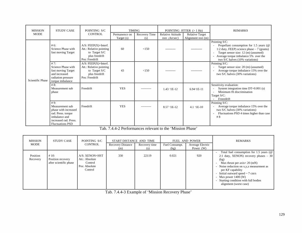
129

TIMING POINTING JITTER (> 1 Hz)MISSIONMODE

STUDY CASE POINTING S/CCONTROL Permanence on

Target (s)Recovery Time

(s)Relative Attitude

RMS (Arcsec)Relative Target

Alignment RMS (m)

REMARKS

# 6:Science Phase withfast moving Target

A/S: FEEP(X)+Interf.Att.: Relative pointing to Target S/C plus freedriftPos: Freedrift

60 <150 ---------- -----------

Pointing S/C:- Propellant consumption for 1.5 years (@

1:2 duty, FEEP) science phase ∼ 7 (grams)- Target sensor size: 12 (m) (assumed)- Average torque imbalance 5% over the

two S/C halves (10% variations)# 7:Science Phase withfast moving Targetand increasedradiation pressuretorque imbalance

A/S: FEEP(X)+Interf.Att.: Relative pointing to Target S/C plus freedriftPos: Freedrift

43 <150 ---------- -----------

Pointing S/C:- Target sensor size: 20 (m) (assumed)- Average torque imbalance 15% over the

two S/C halves (30% variations)

# 8:Measurement subphase

Freedrift YES ---------- 1.43 ·1E-12 6.94·1E-11Sessitivity evaluation:

- System integration time DT=0.001 (s)- Minimum fft discrimination

Target S/C:- Freeedrift

Scientific Phase

# 9:Measurement subphase with increasedrad. Press. torqueimbalance andincreased rad. Press.Fluctuations PSD

Freedrift YES ---------- 8.57 ·1E-12 4.1 ·1E-10Pointing S/C:

- Average torque imbalance 15% over thetwo S/C halves (30% variations)

- Fluctuations PSD 4 times higher than case# 8

Tab. 7.4.4-2 Performances relevant to the ‘Mission Phase’

START DISTANCE AND TIME FUEL AND POWERMISSIONMODE

STUDY CASE POINTING S/CCONTROL Recovery Distance

(m)Recovery time

(s)Fuel Consumpt.

(kg)Average Electric

Power (W)

REMARKS

PositionRecovery

# 10:Position recoveryafter scientific phase

A/S: XENON+HSTAtt.: Absolute ControlPos: Absolute Control

330 22119 0.021 920- Total fuel consumption for 1.5 years (@

2:1 duty, XENON) recovery phases ∼ 30(kg)

- Max thrust per axis= 20 (mN)- Noise reduction on x,y,z measurment as

per KF capability- Initial outward speed ~ 7 cm/s- Max power 1400 (W)- Starting condition with full bodies

alignment (worst case)

Tab. 7.4.4-3 Example of ‘Mission Recovery Phase’

130

- as already mentioned most of the times the dynamic has been propagated at 100 Hz. For case # 3 (withgood control dynamics, a sensitivity has been carried out with propagation at 400 Hz. No basicvariations are observed;

- in alternative to the filter extension technique, it has been tested the method of ‘memory loss’ to copewith inaccuracies (of about +/- 20 %) on some components of the system matrix. The method stabilisethe filter but increases the residual jitter approaching the ones achievable without KF and increases theerror in relative attitude (to 0.02’’-0.03’’). The method of filter extension has been selected.

The performances relevant to the ‘Scientific phase’ are reported in tab. 7.4.4-2 and the followingcomments/considerations apply:

- the Scientific Phase (appropriate sequence of target acquisition and measurement sub phases in full freedrift) is feasible with times of permanence on Target sensor array of some tens of seconds andassuming sensor sizes within technological feasibility (e.g. physical detection grid in the order of 30/40meters in diameter);

- the achievable jitters performances ( for f > 1 Hz), while the Pointing S/C is aligned on the targetsensor array, are extremely low and the resolution on detection of any possible transversaldisplacements of the photon beam used for the scientific part of the experiment, is solely limited by theTarget array resolution capability;

- even assuming an uncertainty factor of 100 on the largest considered basic solar fluctuations (of 40W/m²/√Hz) and imbalance, the resulting jitter at the sensor plane due to system dynamics would be4.1*1E-9 (m) = 0.0041 (µm) still twenty five times larger than the 0.1 (µm) taken as reference.

Performances sensitivity have been done on some parameters/conditions, to summarise:

- the computation of the free drift jitter by propagating the dynamics at 1000 Hz does not presentsignificative changes with respect the propagation at 100 Hz;

- an rough estimation on the minimum resolution achievable in the jitter determination with thepreprocessing/fft method employed, lead to (less then):

- attitude jitter resolution < 5.6109e-017 (arcsec) corresponding to- jitter at sensor plane < 2.8e-015 (m)

An example of performances relevant to the ‘Position Recovery Phase’ are reported in tab. 7.4.4-3 and thefollowing comments/considerations apply:

- the position recovered corresponds approximately to the error accumulated over three hours ofscientific mission in average conditions. The recovery is performed by using ‘high power’ elecricthrusters and in the specific case Xenon thrusters;

- the time necessary for a recovery manoeuver depends on the maximum thrusts (and then electricpower) allowed. In the specific case considered a maximum thrust per axis of 20 (mN) has beenassumed. This, in total, leads to a recovery time approximately twice the preceding free drift time;

- the electric power needed for the thrusters is considerably higher than for the sole attitude control andthe deployment (and subsequent recovery) of dedicated small size solar panel is considered;

- the amount of total fuel consumption needed for 1.5 years mission is 30 kg and such not to significantlychange the inertias of the S/C.

131

8. CONCLUSIONS

The extrordinary possibilities offered by the space environment and the progressive improvements in spacerelated technologies, open to new potential scenarii for performing in orbit experimentation related to basicphysics issues.Line of Sight relative control of a Pointing S/C to a distant Target S/C can be performed with very highperformances even if the position of the two S/Cs and the attitude of the Pointing one are disturbed by externalcauses and without requiring large dimensions of the Pointing S/C (for large optical baseline measurmentsensors). For example, considering two reference S/Cs in GEO and at a nominal distance in the order of 10000(km) during the sustained alignment phases of the Pointing S/C toward the Target S/C, the following range ofcharacteristics appears achievable (with different modality of control and gains):

Target S/C interception error ~ 0.27 m (relative pointing error of ∼ 0.005 arcsec)Target S/C interception jitter (in the band f > 1 Hz) ~ 2 µ m

When the alignment is reached and stable if the relative control is disabled, leaving the S/Cs in free drift mode,the Line of Sight relative jitter (in the band f> 1 Hz) will drop to somethig in the order of:

Target S/C interception jitter (in the band f> 1 Hz) ~ 0.0001 µ m

and this condition could be exploited to perform scientific experimentation requiring exceptionally smoothrelative conditions.

Very important issues in order to achieve above performances are the on board availability of direct relativeattitude measurments (with performances far below the arcsec level) and ultra low noise thrusters.

Relative attitude sensors based on wavefront splitting interferometry, here considered, constitute a verypromising technique for the future missions involving two or more Spacecrafts to be relatively controlled. Thetechnique utilizes flat reflectors only which in principle can be manufactured with extreme flatness.This characteristic, in conjunction with the ever increasing CCD technology and in combination with highefficiency centroiding algorithms, allows for potential performances likely superior the those achievable bymeans of more classical techniques like telescope (employing non flat reflectors) plus quadrant photodiode.Of course the final performances of these interferometer systems will depend on other parameters of which ofprimary importance are the dimensional stability against changing envioronmental conditions as well asdeformation following launch. To exploit full performances it will be necessary to implement an internalmetrology system in a manner similar to multitelescope techniques for astrometric missions.Also the physical size of the interferometer, specifically diameter and length, plays an important role for thefinal performances. For interferometers all contained on board a single spacecraft and with optical baselines inthe order of some decimeters, relative attitude measurement accuracies in the range of the fraction ofmilliarcsecond can be confidently achieved.

The thrusters are very important elements to achieve the performances in target acquisition and keeping mode.Of the evaluated types, FEEP based ones present ideal characteristics of very low noise, throttability and highspecific impule and have been taken as reference for the performances evaluation.

Another important issue is the availability of information with very low noise. On line dynamic filtering isquite effective but the uncertainties on both the distribution matrices and the system matrix need due attention.For the level of performances here considered the straight application of ‘loss of memory techniques’, althougheffective for system stability, tend to reduce the level of noise suppression. Modified filter with integrationaction and addition of extended states for the remaining sensible parameters allow for very good performances.

132

The reachable accuracies could be exploited to perform relativistic type experimentation related to light beamtransversal displacement detection as shown herebelow:

Three spacecraft would be involved one of which, the Pointing S/C, to be exceptionally well aligned to thetarget S/C.This mission is aiming at a tentative approach to detect possible non symmetries of the fundamental space-timetensor caused by electro magnetic fields generated, in the considered experiment, at the Distorter S/C. In thisrespect the considered reference mission would represent a complementary scenario with respect to the moststudied and well known relativistic missions LISA (gravitational wave detection) and Gravity Probe B (gravitomagnetism detection – inertial drag).

Gun S/C

Distorter S/C

Target S/C

Laser Beam

GEO Orbit

Thousands of kilometers Tens of meters

Detector array

ANNEX 1

133

EVALUATION OF PRESENT MISSION SCENARII AND REQUIREMENT RANGE

1 INTRODUCTION

In this Annex 1 a number of significative space missions are presented and discussed in order to have a firstindication on the range of performances (primarily pointing and control) presently considered for the mostdemanding scenarios. The missions described are of scientific type and cover the period 1990-2010approximately; some of them have therefore already been launched, and are operative, while others are still in astudy definition phase. For the missions not yet launched, and of course for the ones still in a definition phase,the presented data can be subject to modifications.

The missions considered have been the following:- Hubble Space Telescope (HST);- Cassini/Huygens;- X-ray Multy-mirror Mission (XMM);- Gravity Probe B;- Space Infrared Telescope Facility (SIRTF);- Next Generation Space Telescope (NGST);- Laser Interferometer Space Antenna (LISA);- Hyper Precision Atom Interferometry in Space (HYPER);- Micro Arcsecond X-ray Imaging Mission (MAXIM Pathfinder);- Darwin Mission

2 MISSIONS DESCRIPTION

2.1 Hubble Space Telescope (HST)

The Hubble Space Telescope is an astronomical platform for observations in the visible/ultraviolet/nearinfrared bands. Its main scientific objectives are:

- investigate the composition, physical characteristics and dynamics of celestial bodies;- examine the formation, structure and evolution of stars and galaxies;- study the history and evolution of the universe;- provide a long term space based research facility for optical astronomy.

The scientific instruments equipping the platform are the following:- Faint Object Camera (FOC);- Space Telescope Imaging Spectrograph (STIS);- Wide Field Planetary Camera (WFPC);- Near Infrared Camera and Multy Object Spectrometer (NICMOS);- (one of the) Fine Guidance Sensor (FGS) for astrometry and photometry.

The HST (shown in fig.2.1-1) can perform target acquisition and tracking of distant objects as well as objectsbelonging to the solar system and is presently the operative most performing platform in term of pointingcapability.

ANNEX 1

ANNEX 1

134

The fine pointing control of HST is performed by using the following basic elements (Ref.[1], [2]):- Fine Guidance Sensors (FGS)-total of three on board;- Accelerometers-total of six rate gyros on board;- Reaction wheels to achieve three axis stabilisation-total of four on board.

Fig 2.1-1 Picture of the HST Fig. 2.1-2 Schematics of FGS

The key component for pointing is the FGS (see also fig.2.1-2), an optical sensor operating between 467 nm to700 nm, which exploits a small amount of the outer portion of the HST field of view (5’’x5’’ of selectedregions within a 69 arcminsquare allowed). The FGS operate as a stellar interferometer locking onto a GuideStar and measure its position (two angles) with an accuracy of 0.0028 (arsec) by tracking its interferometersfringes. The Guide Star is selected from a Guide Star Catalogue, a collection of about 18 million of objects to14.5 visible magnitude. Two of the three FGS are usd for full attitude determination while the thir one, beingso performant, is used as scientific instrument. Each FGS has a mass of 220 kg.

The typical pointing performances of the HST in Fine Lock pointing of distant object are:- pointing accuracy < 0.01 arcsec;- pointing jitter < 0.007 arcsec (rms).

The HST is characterised by:- Dimensions: D=4.3 m, L=13.3 m;- Mass: 10800 kg;- Orbit: LEO 590 km, 28°;- Launch date: 1990.

2.2 Cassini/Huygens

Cassini/Huygens is a Spacecraft launched to perform scientific investigation of the Saturn system (Saturnsurface/athmosphere, rings, moons). The Spacecraft is formed by two main vehicles (see fig. 2.2-1), theOrbiter and the Huygens probe.

ANNEX 1

135

The Spacecraft will reach the Saturn system after more than six years cruise and exploiting a Venus-Venus-Earth-Jupiter gravity assist orbit (VVEJ). The Huygens probe will then separate for its descent to the moonTitan, for in situ scientific measurment, while the Orbiter will begin its remote sensing activity carried outduring the foreseen 74 planet orbits.

Fig 2.2-1 Cassini/Huygens Spacecraft: the Orbiter and Huygens probe.

The fine pointing control of the Spacecraft (basically the Orbiter) is performed during cruise and during remotesensing activity by utilising the following basic elements (see Ref [4] and [5]):

- Stellar Reference Unit (SRU);- Inertial Reference Unit (IRU);- Reaction Wheels.

The key component for pointing is the SRU, an accurate Star Tracker with the followin key features:- FOV 15°;- Accuracy < 4arcsec bias,

< 6 arcsec noise and capable to track 3 to 5 stars simultaneously from a ‘catalogue’ of about 5000 stars.Three IRU are present on board, two operational and one as backup. Each IRU comprises four solid stategyroscops of Hemispherical Resonator type (HRG).The overall pointing performances of the whole Spacecrat are expected in the 10 arcsec range.The Cassini/Huygens Spacecraft is characterised by:

- Dimensions: L=6.8 m;- Mass: 5600 kg (initial, about 50% propellant);- Orbit: interplanetary, VVEJGA gravity assisted (Venus-Venus-Earth-Jupiter);- Launch date: 1997.

2.3 X-ray Multi-mirror Mission (XMM)

XMM spacecraft is an astronomical platform aiming at distant X-ray sources for long observation periodsschematically shown in fig. 2.3-1.

It basically consistes of a quite big telescope installing three mirror modules (see fig 2.3-2 for an explodedview) which is kept pointed to distant targets with high accuracy. The information collected by the mirrors areprocessed by:

- Optical Monitor (OM);- Charged Coupled Devices placed at primary focus (EPIC cameras);- Charged Coupled Devices placed at secondary focus (RGS cameras).

ANNEX 1

136

The XMM fine pointing control at distant target is performed utilising the following basic elements (see alsoRef [5], [6]):

- Star Tracker Telescopes (two);- Inertial Sensors;- Reaction wheels (four).

The measured Star Tracker accuracy has been (beginning of life):- bias ∼ 1.5 arcsec (2σ)- noise ∼ 0.3 arcsec (2σ)

XMM is controlled in attitude with a Relative Pointing Error over 2 minutes at sub arcsec level.

Fig 2.3-1 XMM Spacecraft pictorial view Fig 2.3-2 XMM exploded view

XMM Spacecraft is characterised by:- Dimensions: L=10 m;- Mass: 3800 kg;- Orbit: higly elliptical

Apogee 114000 (km) / Perigee 7000(km)Inclination 40°;

- Launch date: 1999.

2.4 Gravity Probe B

Gravity Probe B (GP-B) is a scientific platform primarily developed to test two of the key predictions of thegeneral relativity:

- the “geodetic” precession of gyroscopes;- the “inertial drag” produced by the earth rotation.

The Spacecraft, described below in more detail, contains exceptionally stable gyroscopes whose tiny changes inspin direction reveals the two mentioned phenomena (see also Ref.[7], [8], [9], [10]).

The “geodetic” precession of gyroscopes (definitively the less important of the two effects) is caused by thespin-orbit coupling experienced by gyroscopes orbiting a massive body. This effect for the operative conditionsof Gravity Probe B is ‘fairly large’ and amounts to approximately 6 arcsec/year. It is caused by the warping ofspace time caused by the mass of the main body independent wheter the body rotates or not.

ANNEX 1

137

The “inertial drag”, sometimes called gravitomagnetic effect, is due to the rotation of the earth and representshow earth drags the local space-time around it because of its spin. In principle an ideal gyroscope suspendedwith no friction above the pole, will not keep its spin axis fixed to the distant stars but will be subject to afleeble rotation drift because of the local dragging of space-time (spin-spin interaction). This effect (whichdepends on the latitude and for which exists an orbital average) amounts to approximately 40 milliarcsec/yearfor the operative conditions of Gravity Probe B and, although discovered in 1917 (Lense-Thirring effect)solving the General Relativity equations around a massive spinning body, has so far never been measured. Theinertial drag is definitively the most important of the two predictions to verify.

Gravity Probe B (see schematics in fig 2.4-1) will orbit the earth on a polar orbit 650 km altitude.

The spacecraft is kept accurately pointed to a Guide Star in two directions while slowly spinning around thestar Line of Sight. The spin direction of the internal gyroscopes are monitored with respect to the Line of Sightand the small deviations integrated and monitored during the 1.5 years foreseen mission. The two effects of“geodetic precession” and “inertial drag” can then be separated.

The key elements of Gravity Probe B, which directly enter in the attitude and orbit control loop, are thefollowing:

- four ‘drift free’ gyroscopes;- a proof mass;- a stellar telescope;- attitude control thrusters.

The four gyroscopes (with the relevant read out devices), the proof mass and the stellar telescope are includedin a block of fused quartz, as shown in fig. 2.4-2, all kept at a temperature of 1.8°K by means of liquid helium,for the whole 1.5 years mission time.

Fig. 2.4-1 Schematics of Gravity Probe B Fig 2.4-2 Quartz block assembly containing gyros, telescopeand proof mass (GP-B)

Each of the four gyroscopes is constituted by a sphere of fused quartz of 38 mm diameter coated niobium (seefig 2.4-3) which becomes a superconductor at liquid helium temperature and allowing the gyroscopes to beelectrically suspended by applying voltages to two saucer shaped electrodes. The gyroscopes are spun at about

ANNEX 1

138

10000 rpm with the spin axis aligned with the axis of the optical telescope and the changes in direction of thespin axis is detected by by means of a Superconducting Quantum Interference Device (SQUID).

The drift rate of such gyroscopes caused by non relativistics effects is < 11

10−

degrees/hour (a total of about 0.5milliarcsec in 1.5 years) sufficient for a good measurement of the investigated relativistics effects.The proof mass is a non spinned mass identical to the sphere-rotor of the gyroscopes and floating in anevacuated cavity near the Spacecraft center of mass. Such a proof mass, being shielded from the externaldisturbances (residual athmosphere, solar radiation pressure) tends to follow an ideal space-time geodetictrajectory; by sensing the position of the proof mass with respect the containment cavity, the Spacecraft is keptby thrusters action to chase the mass always in non contact with it (drag forces free satellite).

The residual non relativistic acceleration of the Spacecraft reduce in such a way to <9

10−

m/s² about 1000 timesbetter than in case such a technique were not used. The perturbances on the accelerometers are therefore alsoreduced.The telescope is implemented as a Cassagrain telescope with aperture of 144 mm a focal lenght of 3810 mmand utilises three mirrors (see fig.2.4-4) and is capable of tracking the Guide Star (Rigel) with accuracies in therange of 0.1-1 milliarcses (on the two pointing directions).

The quartz block assembly (containing the gyroscopes, the proof mass and the telescope) is placed in the mainbody of the Spacecraft designed as Dewar vessel (see fig. 2.4-5) containing about 2300 liters of liquid heliumand capable of keeping cold all instruments for the whole mission.

Fig 2.4-3 Gyroscope picture (GP-B) Fig 2.4-4 Telescope (GP-B)

Fig 2.4-5 Main body of GP-B (designed as Dewar vessel)

ANNEX 1

139

The Spacecraft is spinning at about 0.1-1 rpm around the telescope axis (parallel to the initial gyroscopes axis)so to average the read out errors of gyros and telescope caused by residual disturbances.The force drag free actuation is performed by attitude thrusters utilising the helium boiled off from the dewar.GP-B Spacecraft is characterised by:

- Dimensions: about 2 meters size;- Mass: about 3300 kg (initial life);- Orbit: 650 km, polar- Launch date: end 2002 (expected).

2.5 Space Infrared Telescope Facility (SIRTF)

The Space Infrared Telescope Facility is an astronomical platform aiming at infrared observations of distanttargets and of bodies in the solar system. The observations are carried out by a telescope of 0.85 m diameter, inthe band > 3 micron, supported by three cryogenically cooled (by liquid helium) science instruments for a totalmission duration of 2.5 years. SIRTF platform is illustrated in fig. 2.5-1 and fig. 2.5-2.The pointing control of SIRFT is performed by using the following basic elements (Ref.[11], [12],[13]):

- High performance Star tracker;- Inertial Reference Unit;- Reaction wheels to achieve three axis stabilisation-total of four on board.

Fig. 2.5-1 SIRTF pictorial view Fig. 2.5-2 SIRTF outline

The Star Tracker has a Field of View of 5x5 degrees and is capable to track a minimum of four starssimultaneously and provide an absolute pointing accuracy of 1.5 arcsec at an update rate of 2 Hz. It utilises acatalogue of 87000 stars.The expected pointing performances for the Spacecraft are:

- accuracy < 1.7 arcsec;- jitter < 0.2 arcsec (rms).

SIRFT platform is characterised by:- Dimensions: D=3.5 m, L=1.3 m (approximatly);- Mass: 900 kg (including liquid helium for cryogenic cooling);- Orbit: Heliocentric receeding earth at 0.1AU/year;- Launch date: 2003 (expected).

ANNEX 1

140

2.6 Next Generation Space Telescope (NGST)

The Next Generation Space Telescope can be considered the successor of the Hubble Space Telescope andconsists of a passively cooled 6 m class telescope (8 m goal) aiming at visible and infrared observation of bothdistant targets and objects of the solar system. The goal imaging spectral band is 0.35 to 40 µm. The telescope,and the associated mission, is presently in a definition phase and several approaches have been studied. Apossible telescope schematic is shown in fig. 2.6-1 (see Ref.[14],[15],[16]) and such a configuration isconsidered for the present discussion.

Fig. 2.6-1 NGST possible configuration

With respect to the Hubble Space Telescope, three major differences are foreseen:- the collecting area is about ten times larger and is realised via a deployable primary mirror

approach;- the overall structure is much larger and need be deployed after launch;- the orbit is far from earth and the telescope cannot be serviced after launch.

The mirror modes for such a Spacecraft have quite low resonance frequencies as shown in fig. 2.6-2 and thisfavour a pointing control approach different from the one utilised for the Hubble Space Telescope (with mirrorsmode 60-80 Hz).In case of NGST, the optical pointing stability is achieved by means of a nested loop design involving aninertial Attitude Control System and a Fast Steering Mirror.

The Attitude Control System (ACS) is in charge to provide a stable pointing of the Spacecraft bus by utilisingStar Trackers, Accelerometers and Reaction Wheels all co-located at the Space Support Module. This lowbandwidth loop (0.025 Hz) provides a payload reference frame stable to the arcsec level.

The Fast Steering Mirror (FSM), a rotationally balanced 2 degrees of freedom mechanism, is in charge tomaintain a stable and accurate optical pointing to a Guide Star within few milliarcsec. The FSM has a controlbandwidth of 6Hz and is in charge to suppress the low frequencies disturbances not controlled by the ACS andnot filtered by the isolation trusses. The FSM is located in the Science Instrument module.

The Guide Star sensing can be achieved by using part of the FOV of the telescope. An approach could besimilar to the HST where at any one time a very small FOV (5’’x5’’) is selected out of a larger allowed one (69

ANNEX 1

141

arcminsquare) by means of a moving device. However due to the availability of 4000x4000 pixel large arrays,a fixed size FOV of 3x3 arcmin can be usd for the NGST. Other solutions based on separate guide telescopeshave been discarded because of potential misalignments with respect to the LOS of the main telescope.

Concerning the orbit a candidate proposal is a Lissajous orbit at the Lagrangian L2 point (see schematics in fig.2.6-3) which require a limited deltaV for keeping (although L2 ‘exact’ orbit is unstable). Other alternatives arebeing investigated.

Fig 2.6-2 NGST primarystructural modes

Fig. 2.6-3 NGST possible operative orbit

As presently foreseen (the mission in under definition), the NGST platform can be (preliminary) characterisedby:

- Dimensions: Telescope primary mirror D=6-8m (when deployed);Shield D=15-20 m (when deployed);

- Inertia: 20000 kgm2 (when deployed);- Orbit: Lissajous at L2 non serviceable;- Launch date: 2007 (expected).

2.7 Laser Interferometer Space Antenna (LISA)

LISA mission is being studied with the aime of detecting Gravitational Waves and is basically constituted by agigant Space Interferometer as schematically shown in fig. 2.7-1.LISA mission consists of (see Ref.[17],[18],[19]) a constellation of three identical Spacecrafts placed 5E6 kmapart on the apex of an equilateral triangle. Each of the Spacecrafts has a cilindrical shape realised through astructure made of graphite-epoxy carbon fibre so to minimise thermal expansion effects as schematically shownin fig. 2.7-2.The center of this Spacecraft constellation run an Heliocentric orbit at 1AU and is located 20° behind earth.Due to the particular orbit the triangular formation is maintained throughout the year with the Spacecrafts (sothe triangle) appearing to rotate about its center once a year as schematically shown in Fig. 2.7-3.

ANNEX 1

142

Fig 2.7-1 Pictorial view of LISA missionFig 2.7-2 LISA Spacecraft schematics (three

Spacecrafts identical)

Fig 2.7-3 Orbital features of LISA constellation

Internally to the cilindrical structure is located the Y shaped Scientific Payload (see fig 2.7-4) and a visiblecircular radiator plate.

Fig 2.7-4 Y shaped Payload schematics

ANNEX 1

143

The Payload is formed by two identical Optical Assemblies each containing a T/R Laser Telescope of 30 cmdiameter pointing to one of the other two Spacecrafts, and implementing an interferometric scheme capable todetect variations of the ‘distance between the Spacecrafts’ as accurate as 10E-11 m sufficient to measure thedistance variations between the spacecrafts caused by the flleble fluctuations of the fundamental tensoroccuring during the passage of the gravitational wave. Each of the two Optical Assembly include a proof mass.A more detailed schematics of the Optical Assembly is shown in fig. 2.7-5.

Fig 2.7-5 Internal details of the Optical Assembly

The basic operations performed are herebelow summarised:- each laser of the optical assembly has a power of 1 W continuous in the near infrared and is pointed

to one of the other two spacecrafts. The laser beam is received at the receiver telescope (some pWpower) and used to phase lock the local laser source which is the retransmitted back with full 1Wpower;

- the same happen for the other direction;- the distance taken as reference for the measurments is between the proof masses that are following

a ‘geodetic line’. By performing interferometric measurments between the two interferometer sidesis possible to reveal the passage of a gravitational wave;

- each Spacecraft is kept in the right position by controlling it around its proof masses in order tocompensate for the external disturbances of non gravitational nature;

- the relative attitude is measured by means of incoming laser wave front;- the actuators utilised for Spacecraft position and attitude control are based on FEEP technology

allowing very low thrusts level with accurate control capabilities.

The expected performances for the LISA system are of the following type: Relative attitude pointing:

Achieved via Laser wave front direction technique with expected performances: - stability < 0.002 arcsec - jitter < 0.002 arcsec/vHz

Spacecrafts geodetic positioning:Achieved through 2 proof masses on each Spacecraft with expected performances: - Residual inertial noise < 3*10E-14 m/s2/vHz

-Spacecraft position control w.r.t the inertial mass <10E-8 m Accuracy of the interferometric distance measurment system between any two Spacecrafts (indeed

between proof masses of the Spacecraft) <10E-11 m with the masses at 5E6 km apart.

ANNEX 1

144

Each LISA platform is (preliminary) characterised by:- Dimensions: flat cylinder D=1.8 m, H=0.5 m (approximatly);- Mass: 265 kg (operational, 30% contingency included);- Orbit: Heliocentric with triangular constellation formation;- Launch date: 2010 (expected – study phase).

2.8 Hyper Precision Atom Interferometry in Space (Hyper)

The Hyper mission (see Ref.[20]), presently in a preliminary study phase, will have the following mainscientific objectives:

- mapping the frame-dragging (gravitomagnetism) effects of the earth, in terms of magnitude andsign, as a function of of the latitude;

- perform basic phisics verifications by determining the fine structure constant and investigatedistinct sources of matter-wave decoherence.

The Spacecraft, schematically depicted in fig. 2.8-1, is planned to be placed in a sun synchronous orbit at 700km altitude.

Fig. 2.8-1 Pictorial view of Hyper S/C

With reference to the mapping of the gravitomagnetic field, the Spacecraft will be kept pointed to a referenceGuide Star and the drift (of gravitational nature) experienced by the very accurate on board gyroscopes willprovide the information on the frame dragging effect.The basic basic elements utilised for the pointing control and gravitomagnetic measurments are:

- Electric propulsion thrusters;- Star telescope;- Gyroscopes and Accelerometers;- Proof Masses.

The electric propulsion is foreseen to be accomplished by 16 FEEP type thrusters sized for 500µN max thrusteach. The Star telescope keeps tracking of a reference Guide Star with an accuracy < 0.02 arcsec and is basedon a Cassegrain approach.

The real technological issue is related to the gyroscopes and accelerometers. Indeed Hyper carry four cold atominterferetometers, which exploit atom-laser light interaction, and in which the drift velocity of the atoms can bereduced to 20 cm/s (at an atom temperature of 1µ°K). These four interferometers can be configured to form two

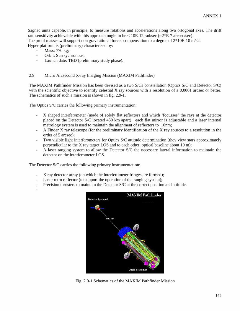
ANNEX 1

145

Sagnac units capable, in principle, to measure rotations and accelerations along two ortogonal axes. The driftrate sensitivity achievable with this approach ought to be < 10E-12 rad/sec (≅2*E-7 arcsec/sec).The proof masses will support non gravitational forces compensation to a degree of 2*10E-10 m/s2.Hyper platform is (preliminary) characterised by:

- Mass: 770 kg;- Orbit: Sun sychronous;- Launch date: TBD (preliminary study phase).

2.9 Micro Arcsecond X-ray Imaging Mission (MAXIM Pathfinder)

The MAXIM Pathfinder Mission has been devised as a two S/Cs constellation (Optics S/C and Detector S/C)with the scientific objective to identify celestial X ray sources with a resolution of a 0.0001 arcsec or better.The schematics of such a mission is shown in fig. 2.9-1.

The Optics S/C carries the following primary instrumentation:

- X shaped interferometer (made of solely flat reflectors and which ‘focusses’ the rays at the detectorplaced on the Detector S/C located 450 km apart); each flat mirror is adjustable and a laser internalmetrology system is used to maintain the alignment of reflectors to 10nm;

- A Finder X ray telescope (for the preliminary identification of the X ray sources to a resolution in theorder of 5 arcsec);

- Two visible light interferometers for Optics S/C attitude determination (they view stars approximatelyperpendicular to the X ray target LOS and to each other; optical baseline about 10 m);

- A laser ranging system to allow the Detector S/C the necessary lateral information to maintain thedetector on the interferometer LOS.

The Detector S/C carries the following primary instrumentation:

- X ray detector array (on which the interferometer fringes are formed);- Laser retro reflector (to support the operation of the ranging system);- Precision thrusters to maintain the Detector S/C at the correct position and attitude.-

Fig. 2.9-1 Schematics of the MAXIM Pathfinder Mission

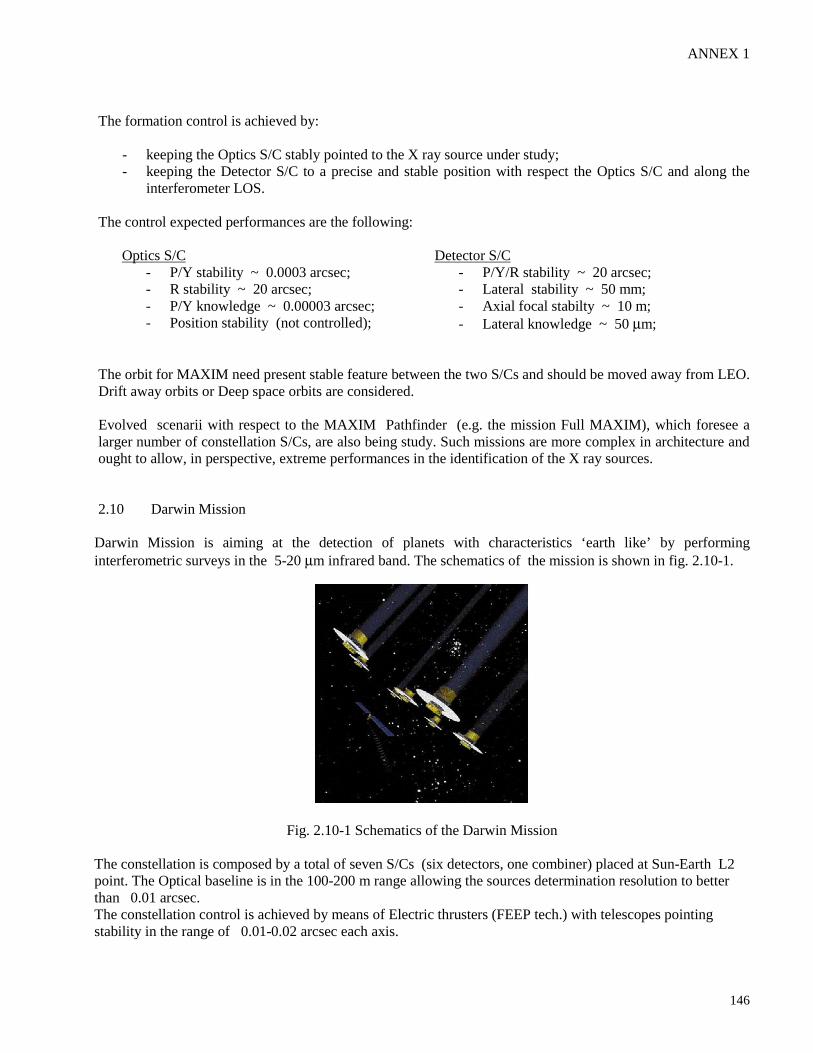
ANNEX 1

146

The formation control is achieved by:

- keeping the Optics S/C stably pointed to the X ray source under study;- keeping the Detector S/C to a precise and stable position with respect the Optics S/C and along the

interferometer LOS.

The control expected performances are the following:

Optics S/C- P/Y stability ~ 0.0003 arcsec;- R stability ~ 20 arcsec;- P/Y knowledge ~ 0.00003 arcsec;- Position stability (not controlled);

Detector S/C- P/Y/R stability ~ 20 arcsec;- Lateral stability ~ 50 mm;- Axial focal stabilty ~ 10 m;- Lateral knowledge ~ 50 µm;

The orbit for MAXIM need present stable feature between the two S/Cs and should be moved away from LEO.Drift away orbits or Deep space orbits are considered.

Evolved scenarii with respect to the MAXIM Pathfinder (e.g. the mission Full MAXIM), which foresee alarger number of constellation S/Cs, are also being study. Such missions are more complex in architecture andought to allow, in perspective, extreme performances in the identification of the X ray sources.

2.10 Darwin Mission

Darwin Mission is aiming at the detection of planets with characteristics ‘earth like’ by performinginterferometric surveys in the 5-20 µm infrared band. The schematics of the mission is shown in fig. 2.10-1.

Fig. 2.10-1 Schematics of the Darwin Mission

The constellation is composed by a total of seven S/Cs (six detectors, one combiner) placed at Sun-Earth L2point. The Optical baseline is in the 100-200 m range allowing the sources determination resolution to betterthan 0.01 arcsec.The constellation control is achieved by means of Electric thrusters (FEEP tech.) with telescopes pointingstability in the range of 0.01-0.02 arcsec each axis.

ANNEX 2

147

Extract from the Seminar held on November 2002 on:

“Conceptual Investigation of a Relativistic In Orbit Experiment Mission RequiringVery Demanding S/Cs Relative Control”

Summary of some significant cases

1. Motivations and Ojectives

This Annex 2 summarises some of the representative outcomes of the conceptual investigation of aRelativistic in orbit experiment mission evaluated in the frame of the ‘Dottorato di Ricerca (PhD)’ carriedout on the main subject of:

“ Methodologies for Accurate Spacecrafts Relative Control in Support to Very Demanding ScientificMissions”

The presented experiment is intended as a possible scenario from which to derive a challanging range ofrequirements for the key technological topic of the PhD research.For more detailed information reference is made to documents [55] and [56] related to the seminar activityforeseen the second year of the Doctorate School.

Reference experiment missionThe mission considered is aiming at some indications in support to the presumed unified nature of thegravitation and electromagnetic fields.The unified theories revised for this purpose have been the ones based on a four dimensional continuumspace-time non-Riemannian and in general endowed by a non symmetric fundamental tensor gαβ and a non-

symmetric connection Γ βγα . The key investigated aspect was how to reveal a possible non symmetry of the

fundamental tensor, and of the connection coefficients, in relation to the presence of electro/magnetic fields.The topic of field unification is extremely challanging and no consensus has been so far reached within thescientific community on the interpretation of the Unified Field Equations proposed by Einstein and othersboth in the basic formulation and in the possible variants with sources. However the impressive andprogressive achievements in space technology may allow to conceive future space operational scenariiwhich may support some possible verifications on such a challanging subject.

2. Fundamentals and Field Equation Structure

General Relativity

The theory is based on a symmetric fundamental tensor gαβ and a symmetric connection γαβΓ of a Riemann

space:

−=−

=

−

−

∂∂

=

αβαβαβ

γ

δ

βαδγ

δ

αδβγαβ

γαβ

χTRgR

ggx

gg

2

1

0;

ANNEX 2

ANNEX 2

148

Equation provides the link between the connection coefficients

γ

δ

α , in this case the Christoffel

symbols of the Riemann space, and the fundamental tensor αβg .

Equation is the field equation. It links the fundamental tensor αβg (which describes the gravitational field

and enters in the contracted curvature tensor αβR ) to the matter total energy/momentum tensor αβT .

Einstein Unified Field

The theory assumes a non symmetric fundamental tensor gαβ and a non symmetric connection γαβΓ :

=→=

=→=

=

=Γ−Γ−∂∂

=−+

)0 t to(equivalen 0

)0 t to(equivalen 0

0

0

],[][

][

)(

βγδβγδαβγδ

αβαβ

αβ

δγβαδ

δαγδβγ

αβγαβ

ε RR

Sf

R

ggx

gg

Equation provides link between the connection coefficients Γβγα and the fundamental tensor gαβ .

Formally it differs from the equivalent equation of general relativity by the presence of polarisation +/- in thecovariant derivative of gαβ ; the polarisation is now possible because of the asymmetries in gαβ and Γβγ

α .Equation is the first of the three field equations and can be seen as an extension of the only field equationof General Relativity. Equations and are the remaining two field equations and play the role ofgeneralized Maxwell equations.All three field equations contain both the symmetric part ( )g αβ and the skew symmetric part [ ]g αβ of the

fundamental tensor.

Einstein Unified Field with sources appended

These are basically the Einstein unified equation to which ‘source term’ have been appended. One exampleof formulation is the following:

( )

( )

=++

−=

−=

+−=−+

αβγαβγβγαγαβ

αβ

αβ

γηγη

αβαβαβ

γηαβγβαηηβαγα

ηαβ

π∂

∂

π

π

KRRR

jgx

g

TssTR

ggggggjg

],[],[],[

][

)(

][

4g-

2

18

3

4Where αβs is defined by:

( )− = −

=

ss gg

s s

αβ αβ

γδαδ

γαδ

and constitute the fundamental tensor of an intermediateRiemann space.Added sources terms:

αβT = Matter Energy/Momentum tensor

αJ = Electric current four vector

αβγK = Magnetic current four vector

The shown equations maintain a meaning similar to the ones of the unifiedEinstein/Schrodinger field equations even if in this case the formal structure is complicated by the addition

ANNEX 2

149

of sources. The curvature tensor considered is the ‘simmetrised’ one. Above equations reduce to the Einsteinunified ones when no sources are present and are ‘transposition invariant’ even when sources are present.They allow for both electric currents and magnetic currents.

3. Possible Structure of the Equation of Motion

As mentioned in the introductory part no consensus has been so far reached within the scientific communityon the interpretation of the Unified Field Equations. This apply not only to the correlation of the physicalentities to the geometrical ones (e.g. electromagnetic tensors with respect to the skew symmetric part of thefundamental tensor or to the skew symmetric part of the contracted Riemann tensor, structure andsymmetries of the total energy tensor, ….) but clearly also to the equations of motion (for charged or notparticles, photons).

The only case theoretically well accepted is the one relevant to general relativity.

Concerning the equations of motion in the unified space, their final structure ought to be derived by utilisingthe characteristics identities of the space (like the Bianchi identities for the Riemann cases) arriving then to aset of four differential equation. In spaces with fundamental tensor and connection not symmetric thisprocess is quite complex also considering the different possibilities for the interpretation of the physicalentities.For the Unified Space two main assumptions on motion have been evaluated:

- the equation of motion is an autoparallel of the unified space;- the equation of motion is an autoparallel (and null geodesic) of an ‘intermediate’ Riemann space

Equation of motion of a neutral test particle in vacuum: case of General Relativity

The equation of motion are controlled by the following equation:

0T ; =βαβ

where αβT represents the total momentum-energy tensor.Assuming solved the field equation, the motion of neutral particles result in:

==

=

=

+→=

==

) d takingparticles physicalfor ( 1

photons)(for 0with

0d

0

parameter line re whe

i

i

i

mk 2

2

;i

jiij

i

i

mkij

j

ii

dxdxg

d

dx

d

dx

d

x

d

dx

ξλλ

λλξξξ

λλ

ξξ

λ

where:

;= covariant derivative with respect to the Christoffel Symbols

γ

α

β

Above trajectories are autoparallel (and geodesics) of the General Relativity Riemannian Spacetime.

Equation of motion of a neutral test particle in vacuum: case of Unified Space (in the showncase the motion is assumed as an autoparallel of the full connection)

Assuming the motion of a neutral test particle be an autoparallel of the full connection such amotion can be described by:

ANNEX 2

150

Γ=

=Γ+→===

=

−+

i

mki

i

dq

dx

dq

dx

dq

x

qdq

dx

m)(k

m)(k 2

2

connection neutral therespect to with derivativeCovariant

0d

0

parameter) line=(

ββ

αββ

αβ

β

α

αα

λλλλλλ

λ

Concerning the total connection coefficients , they are described by the following structure:

=+Λ=++

=Γ αβγ

αβγ

αβγ

αβγ

αβγ βγ

α

SSA Total connection coefficients (transforms like

Christoffel symbols)

βγα = Christoffel symbols, symmetric in βγ, associated to )(αβg

αβγ A = Symmetric tensor in βγ (contains αβg effects)α

βγ S = Skew symmetric part in βγ of the total connection (torsion tensor; contains αβg

effects)αβγ Λ = Symmetric part in βγ of the total connection =

αβγ )(Γ = Neutral connection

This type of motion converges to the General Relativity one in case of no electromagnetic field.

Equation of motion of a neutral test particle in vacuum: case of Unified Space (motion assumeddescribed by an autoparallel and geodesic of an intermediate Riemannian space)

Following recent approaches, an intermediate Riemann space endowed with a fundamentatal tensor αβs ,

anyway related to the unified space fundamental tensor, can be introduced as previously described. In case ofnull electric and magnetic currents the equation of motion can take the following form:

( ) ( ) ( ) 0 02

1;

][][

;=−→=−+−=−

βγηβηαγην

νγηγηηαγ

βγηβηαγ TsssggKRjgsTsss

which results into:

0d

0Ti

mk 2

2

; =

+→=

ξξξβ

αβ

d

dx

d

dx

d

x mki

where αβT play the role of the total momentum energy tensor and the Christoffel symbols are associated to

the ijs space.

A situation similar to the General Relativity would result this time applied to the intermediate Riemannspace. Also in this case the motion reduce to the General Relativity one in case no electromagnetic field werepresent.

4. Cases Investigated and Possible Light Beam Transversal Displacement

A possible experimental condition which may provide indications on the subject of non-symmetry of space-time and to the possible structure of the equation of motion, could be based on the following steps:

a highly collimated laser light beam (photons) is fired at a very distant target sensor arraywhere the ‘spot’ can be centroided;

in the initial part of the laser beam trajectory, extremely high electric/magnetic fields (withappropriate geometrical orientations) are applied in confined regions;

upon the application of such fields the spacetime metric can be fleebely distorted renderingthe fundamental tensor slightly non symmeteric;

ANNEX 2

151

the effect of such non symmetries could be a swing in the beam direction that can berevealed as a very small change of the ‘spot’ centroid at the distant target.

The possible structure of a light beam transversal displacement have been studied, based on the previousdiscussion, according to the assumption:

• assumed motion type: autoparallel of the full connection

and, for one specific case, the following has also been investigated:

• assumed motion type: autoparallel and geodesic of an intermediate Riemann space

The evaluations have been carried out for stationary electric and magnetic fields of simple geometries.The motion has been studied inside a ‘distorsion area’ where properly oriented electric/magnetic fields aregenerated. With reference to the following schematics these fields can been oriented in order to have thepossible motion laying on the z-y plane.

x

z

y 1

3

2

Swing s

L

1)= Initial trajectory

2) = Trajectory continuation when

E E E H H Hx y z x y z= = = = = = 0

(at most distorted by the earth gravity field)

3) = Possible distorted trajectory when the electromagneticfield is activated

As far as the mating of the electromagnetic tensor with geometrical entities, the following has beenexplored:

Tensor lFundamenta theofpart symmetric skew the toed tensor tineticElectromag =αβF

For one specific conditions however the following has been investigated:

Tensor Curvature contracted theofpart symmetric skew the totied tensor neticElectromag =αβF

Summary of the reported cases

Two of the significative study cases are summarized in this note and hereafter reported:

• First reported case: it is relevant to a circular field induced by an infinite rectilinear conductor carrying astationary current; here the light beam has been assumed to arrive perpendicular to the conductor and at acertain distance. The motion has been assumed as an autoparallel of the full connection and theelectromagnetic tensor tied to the skew symmetric part of the fundamental tensor;

• Second reported case: it is relevant to a radial field induced by a very long rectilinear conductorelectrically charged; in this case the light beam has been assumed to arrive parallel to the conductor andat a certain distance. The motion has been assumed as an autoparallel of the full connection and twoinvestigations were performed:

- electromagnetic tensor tied to the skew symmetric part of the fundamental tensor;- electromagnetic tensor tied to the skew symmetric part of the contracted curvature tensor.

ANNEX 2

152

4.1 First reported case

This case is relevant to a circular magnetic field induced by a stationary current running in a long rectilinearconductor (coincident with the x axis) according to the following scheme:

Magnetic field structure (b is a known constant):

+⋅−=

+⋅=

)(y

yF

)(y

zF

22z

22y

zb

zb

Assuming the Electromagnetic tensor tied to the skew symmetric part of the fundamental tensor (via anunknown coupling constant B), the fundamental tensor can be computed with exact solution leading to thefollowing:

++−

−−

=

)FBFB(1BFBF0

BF-100

BF-010

0001

g

2z

22y

2zy

z

yij

The connection coefficients will have a limited number of non null terms which can be grouped in the nonsymmetric ones and symmetric ones:

[ ]

[ ]

[ ]

[ ]

⋅∂∂−=Γ

⋅∂∂−=Γ

⋅∂∂

−=Γ

⋅∂∂

−=Γ

Bz

By

Bz

By

Fz

Fz

F

F

343

342

y243

y242

Λ=⋅

∂∂−

∂∂−=Γ

Λ=⋅

∂∂

−∂∂

−=Γ

344

2zz

zy

344

244

2yz

yy

244

BF

FF

F

BF

FF

F

zy

zy

Computation of the trajectory as an autoparallel of the full connection

The autoparallel trajectory can now be computed based on the form previously introduced:

=Λ+

==

0

parameter) line (

i 2

2

ξξξ

ξξ

λ

d

dx

d

dx

d

xd

d

dx

mk

mk

i

ii

z

x y

zLaser beam

∆

ANNEX 2

153

Taking in to account the non null connection terms and referring to the following entrance conditions:

=−∞=∂∂

=−∞=∂∂

0)(

0)(

yy

z

yy

x

and

∆=−∞==−∞= )(

0)(

yz

yx

the trajectory can be written as:

=

=Λ+

=Λ+

=

0)(

0)()(

0)()(

0

2

2

3 442

2

2 442

2

2

2

ξ

ξξξ

ξξξ

ξ

d

ctd

d

ctd

d

ctd

d

zd

d

ctd

d

ctd

d

yd

d

xd

the motion remaining on the yz plane.

Upon substitution of the magnetic field equation, the motion will be described by:

=

+−=

+−=

=

0)(

)()(

)(b

)()(

)(b

0

2

2

22222

2

2

22222

2

2

2

2

ξ

ξξξ

ξξξ

ξ

d

ctd

d

ctd

d

ctd

zy

zB

d

zd

d

ctd

d

ctd

zy

yB

d

yd

d

xd

It is noted that, for the achievable magnetic field strength (even if very high), the possible perturbedtrajectory would be extremely close to the unperturbed one. Furthermore since the interest is in thetransversal displacement (z), above equation can be written as:

≅∆+

∆−=

cty

yB

dy

zd222

222

2

)(b

Above equation can be easily integrated leading to the geometricl profiles with a total angular deflectionreported in table 4.1-1.

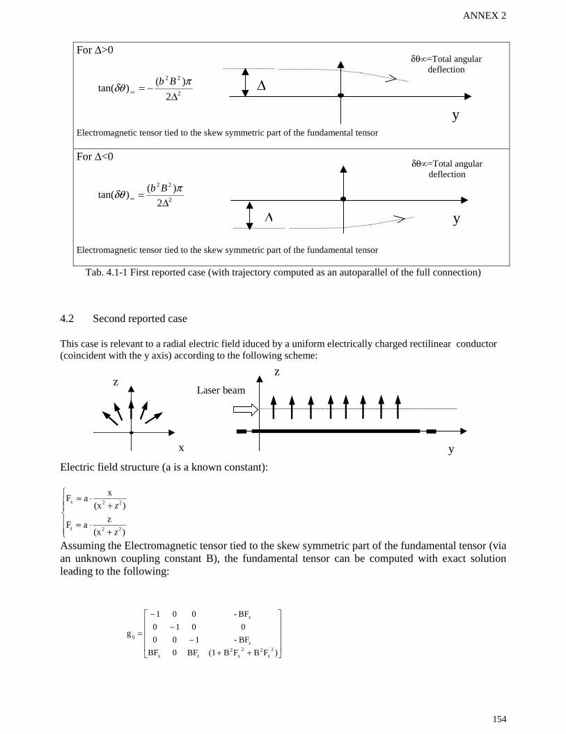
ANNEX 2

154

For ∆>0

2

22

2

)()tan(

∆−=∞

πδθ Bb

Electromagnetic tensor tied to the skew symmetric part of the fundamental tensor

For ∆<0

2

22

2

)()tan(

∆=∞

πδθ Bb

Electromagnetic tensor tied to the skew symmetric part of the fundamental tensor

Tab. 4.1-1 First reported case (with trajectory computed as an autoparallel of the full connection)

4.2 Second reported case

This case is relevant to a radial electric field iduced by a uniform electrically charged rectilinear conductor(coincident with the y axis) according to the following scheme:

z

x

Laser beam

z

y

Electric field structure (a is a known constant):

+⋅=

+⋅=

)(x

zaF

)(x

xaF

22z

22x

z

z

Assuming the Electromagnetic tensor tied to the skew symmetric part of the fundamental tensor (viaan unknown coupling constant B), the fundamental tensor can be computed with exact solutionleading to the following:

++−

−−

=

)FBFB(1BF0BF

BF-100

0010

BF-001

g

2z

22x

2zx

z

x

ij

∆ y

δθ∞=Total angulardeflection

∆

y

δθ∞=Total angulardeflection

ANNEX 2

155

The connection coefficients again will have a limited number of non null terms which can be grouped in thenon symmetric ones and symmetric ones:

[ ]

[ ]

[ ]

[ ]

⋅∂∂−=Γ

⋅∂∂−=Γ

⋅∂∂

−=Γ

⋅∂∂

−=Γ

Bz

B

Bz

B

Fzx

Fz

Fx

F

343

341

x143

x141

⋅

∂∂−

∂∂−=Γ

⋅

∂∂−

∂∂−=Γ

2zz

zx

344

2xz

xx

144

BF

Fx

FF

BF

Fx

FF

z

z

Computation of the trajectory as an autoparallel of the full connectionThe trajectory can now be computed with a similar approach as in the first reported case

The trajectory equation takes the form:

=Λ+

==

0

parameter) line (

i 2

2

ξξξ

ξξ

λ

d

dx

d

dx

d

xd

d

dx

mk

mk

i

ii

Considering the previous results (only two of the i mkΛ are non null) the trajectory would result into:

=

=Λ+

=

=Λ+

0)(

0)()(

0

0)()(

2

2

3 442

2

2

2

1 442

2

ξ

ξξξ

ξ

ξξξ

d

ctd

d

ctd

d

ctd

d

zd

d

yd

d

ctd

d

ctd

d

xd

With the assumed structure for the electric field and taking the following entrance conditions:

==∂∂

==∂∂

0)0(

0)0(

yy

z

yy

x

and

∆====

)0(

0)0(

yz

yx

the resultant trajectory will remain on the yz plane and the connection coefficients can be written as:

==∂∂

==

0),0(

0),0(

zxz

F

zxF

x

x

∂∂

−==Λ

==Λ

z

FFBzx

zx

zz

23 44

1 44

),0(

0),0(

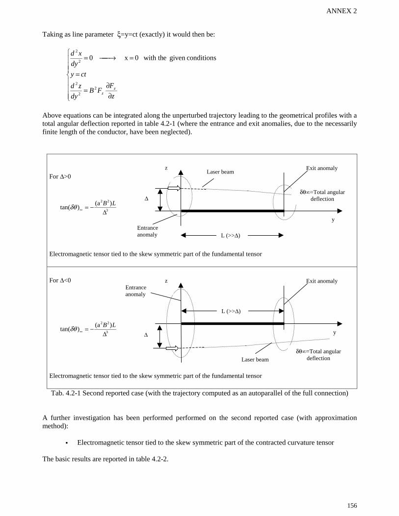
ANNEX 2

156

Taking as line parameter ξ=y=ct (exactly) it would then be:

∂∂

=

=

=→=

z

FFB

dy

zd

cty

dy

xd

zz

22

2

2

2

conditionsgiven e with th0 x 0

Above equations can be integrated along the unperturbed trajectory leading to the geometrical profiles with atotal angular deflection reported in table 4.2-1 (where the entrance and exit anomalies, due to the necessarilyfinite length of the conductor, have been neglected).

For ∆>0

3

22 )a()tan(

∆−=∞

LBδθ

Electromagnetic tensor tied to the skew symmetric part of the fundamental tensor

For ∆<0

3

22 )a()tan(

∆−=∞

LBδθ

Electromagnetic tensor tied to the skew symmetric part of the fundamental tensor

Tab. 4.2-1 Second reported case (with the trajectory computed as an autoparallel of the full connection)

A further investigation has been performed performed on the second reported case (with approximationmethod):

Electromagnetic tensor tied to the skew symmetric part of the contracted curvature tensor

The basic results are reported in table 4.2-2.

z

y

Laser beam

L (>>∆)

Entranceanomaly

Exit anomaly

∆

δθ∞=Total angulardeflection

z

y

Laser beam

L (>>∆)Entranceanomaly

Exit anomaly

∆δθ∞=Total angular

deflection

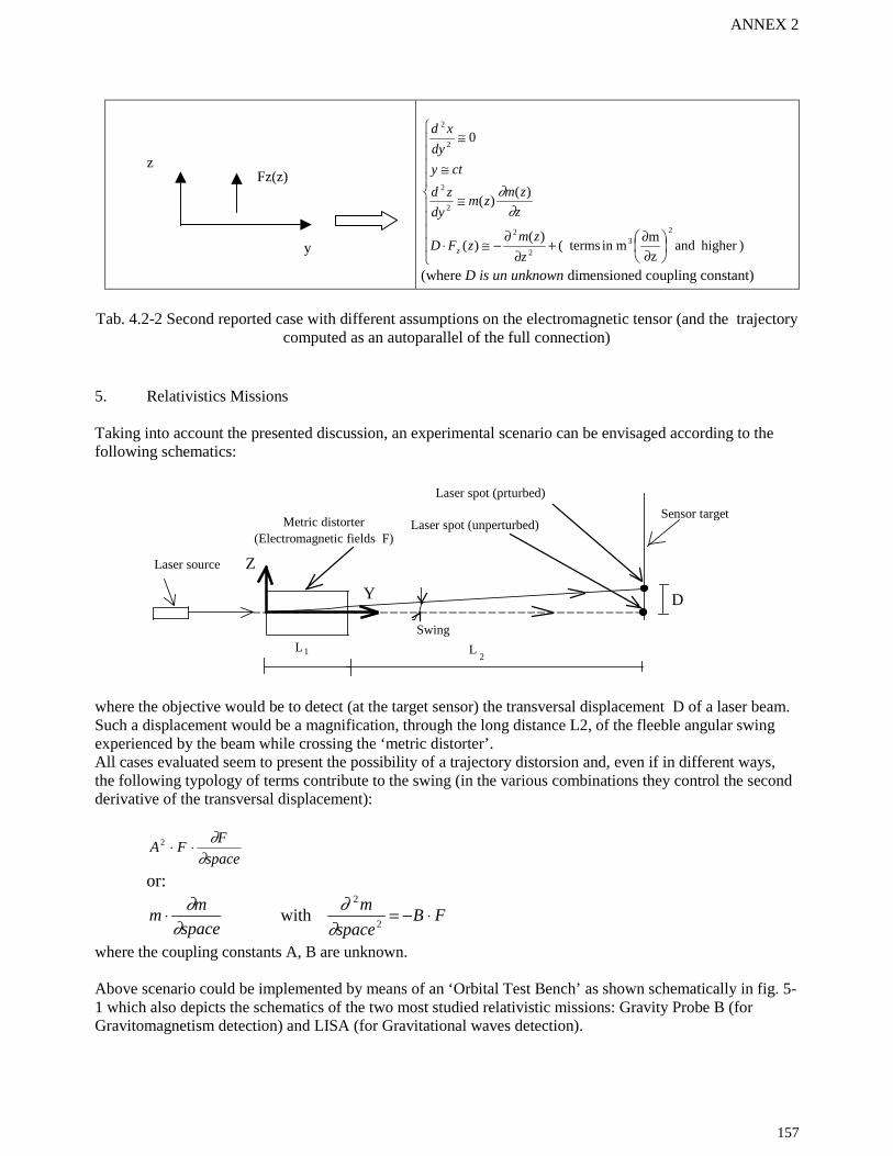
ANNEX 2

157

∂∂+

∂∂

−≅⋅

≅

≅

≅

)higher andz

mmin terms(

)()(

)()(

0

23

2

2

2

2

2

2

z

zmzFD

z

zmzm

dy

zd

cty

dy

xd

z

∂∂

(where D is un unknown dimensioned coupling constant)

Tab. 4.2-2 Second reported case with different assumptions on the electromagnetic tensor (and the trajectorycomputed as an autoparallel of the full connection)

5. Relativistics Missions

Taking into account the presented discussion, an experimental scenario can be envisaged according to thefollowing schematics:

Sensor target

Swing

Metric distorter

Laser source

L 1 2

L

(Electromagnetic fields F)

Laser spot (prturbed)

Laser spot (unperturbed)

Z

Y D

where the objective would be to detect (at the target sensor) the transversal displacement D of a laser beam.Such a displacement would be a magnification, through the long distance L2, of the fleeble angular swingexperienced by the beam while crossing the ‘metric distorter’.All cases evaluated seem to present the possibility of a trajectory distorsion and, even if in different ways,the following typology of terms contribute to the swing (in the various combinations they control the secondderivative of the transversal displacement):

2

space

FFA

∂∂⋅⋅

or:

FBspace

m

space

mm ⋅−=⋅

2

2

with ∂∂

∂∂

where the coupling constants A, B are unknown.

Above scenario could be implemented by means of an ‘Orbital Test Bench’ as shown schematically in fig. 5-1 which also depicts the schematics of the two most studied relativistic missions: Gravity Probe B (forGravitomagnetism detection) and LISA (for Gravitational waves detection).

zFz(z)

y

ANNEX 2

158

Gravity Probe B

Main Objective:Inertial Drag Detection(Gravitomagnetism)

Configuration:one S/C in Polar Orbit

LISA

Main objective:Gravitational Waves Detection

Configuration:three S/Cs constellation at 1AU,30° earth retrograde and 5 milionkilometers apart

Orbital Test Bench for relativisticsverifications

Main Objectives:Support in the evaluation on thepossible electro-gravity unifiedtheories

Configuration:3 S/Cs constellation in GEO

Gun S/C

Distorter S/C

Target S/C

GEO Orbit

Laser Beam

Laser Beam (distorted)

Thousands of kilometers Tens of metersDetector

Fig. 5-1 Schematics of the two most studied Relativistic Missions (Gravity Probe B and LISA) and of theproposed Orbital Test Bench in support to unified theory studies

ANNEX 3

159

Extract from the Seminar held on November 2002 on:

Wave front Interferometric technique for accurate S/C’s relative attitude determination(Summary)

1. INTRODUCTION

This Annex 3 summarises the operational principle and some of the main features of a wavefrontinterferometric technique that can be considered for the implementation of a very accurate relative attitudesensor between Spacecrafts.

This specialistic activity has been performed in the frame of the ‘Dottorato di Ricerca (PhD)’ degree activitycarried out on the main subject of:

“ Methodologies for Accurate Spacecrafts Relative Control in Support to Very Demanding ScientificMissions”

For more detailed information reference is made to document [35] related to the seminar activity foreseen thesecond year of the Doctorate School.

2. INTERFEROMETER APPROACH BASED ON FLAT REFLECTORS

The interferometer considered is of wavefront splitting type capable to operate in the application schemerepresented in Fig.2-1.

(Two dimensional drawing: only pitch angle shown)

Fig. 2-1 Application scheme for the considered interferometer

The two key elements determining the performances in terms of pitch and yaw information are theinterferometer located on the Pointing S/C and the quality of the laser beam casted by the Target Spacecraft.

Target S/C

Laser beam

Pointing S/C(Interferometer)

Beam Wavefron(Coherence)

α (Pitch)

Pointing Direction

Wavefront Intakes

ANNEX 3

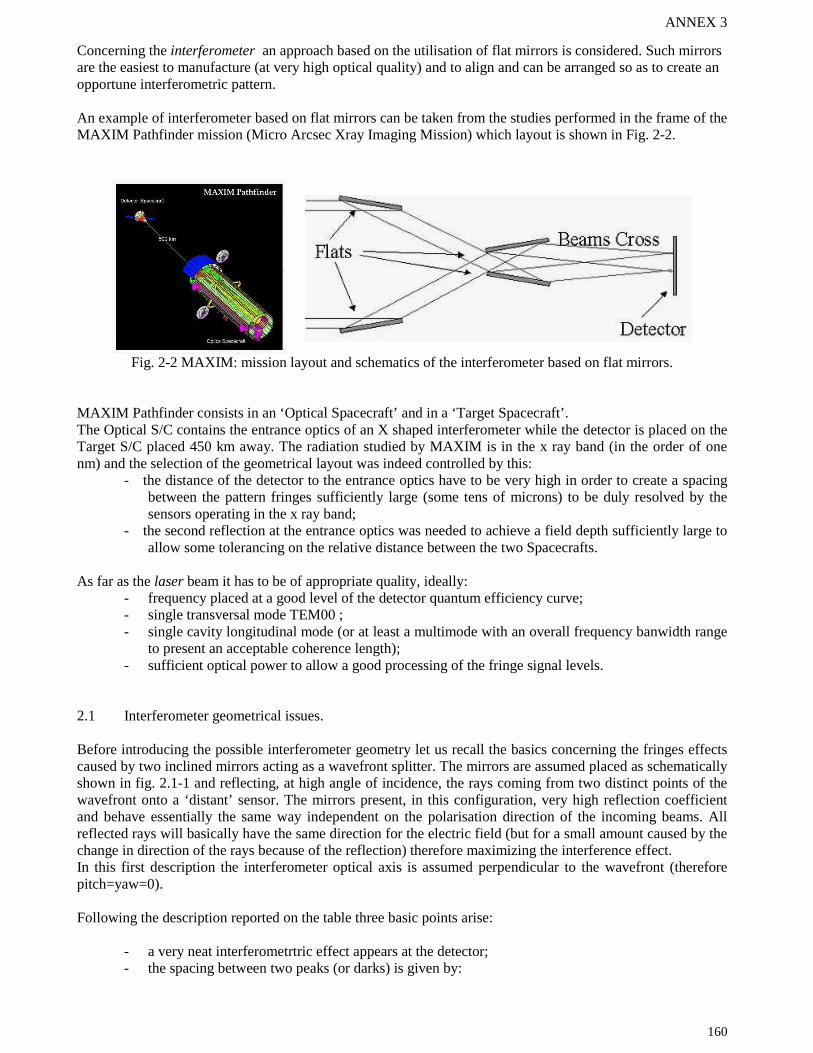
ANNEX 3

160

Concerning the interferometer an approach based on the utilisation of flat mirrors is considered. Such mirrorsare the easiest to manufacture (at very high optical quality) and to align and can be arranged so as to create anopportune interferometric pattern.

An example of interferometer based on flat mirrors can be taken from the studies performed in the frame of theMAXIM Pathfinder mission (Micro Arcsec Xray Imaging Mission) which layout is shown in Fig. 2-2.

Fig. 2-2 MAXIM: mission layout and schematics of the interferometer based on flat mirrors.

MAXIM Pathfinder consists in an ‘Optical Spacecraft’ and in a ‘Target Spacecraft’.The Optical S/C contains the entrance optics of an X shaped interferometer while the detector is placed on theTarget S/C placed 450 km away. The radiation studied by MAXIM is in the x ray band (in the order of onenm) and the selection of the geometrical layout was indeed controlled by this:

- the distance of the detector to the entrance optics have to be very high in order to create a spacingbetween the pattern fringes sufficiently large (some tens of microns) to be duly resolved by thesensors operating in the x ray band;

- the second reflection at the entrance optics was needed to achieve a field depth sufficiently large toallow some tolerancing on the relative distance between the two Spacecrafts.

As far as the laser beam it has to be of appropriate quality, ideally:- frequency placed at a good level of the detector quantum efficiency curve;- single transversal mode TEM00 ;- single cavity longitudinal mode (or at least a multimode with an overall frequency banwidth range

to present an acceptable coherence length);- sufficient optical power to allow a good processing of the fringe signal levels.

2.1 Interferometer geometrical issues.

Before introducing the possible interferometer geometry let us recall the basics concerning the fringes effectscaused by two inclined mirrors acting as a wavefront splitter. The mirrors are assumed placed as schematicallyshown in fig. 2.1-1 and reflecting, at high angle of incidence, the rays coming from two distinct points of thewavefront onto a ‘distant’ sensor. The mirrors present, in this configuration, very high reflection coefficientand behave essentially the same way independent on the polarisation direction of the incoming beams. Allreflected rays will basically have the same direction for the electric field (but for a small amount caused by thechange in direction of the rays because of the reflection) therefore maximizing the interference effect.In this first description the interferometer optical axis is assumed perpendicular to the wavefront (thereforepitch=yaw=0).

Following the description reported on the table three basic points arise:

- a very neat interferometrtric effect appears at the detector;- the spacing between two peaks (or darks) is given by:

ANNEX 3

161

λ⋅=D

LPs

λ=light wavelength L=interferometer length D=interferometer inpot diameter;

- the spacing is therefore magnified with respect to the wavelength and this will be very importantin view of the pixel size of the detector.

The fringe shaping which appears in this case is along one direction only and it would feel only pitch attitudevariations (with the absolute information practically lost as soon as a pitch value of λ/D is achieved).

To overcame such limitations, as well as to increase the peaks of irradiance at the detector, a multiple mirrorapproach is used.Several geometry schematics have been considered as shown in fig. 2.1-2 and they foresee the utilisation of 1,4, 8 and 16 pairs of symmetrically placed mirrors. The field at the detector is therefore the contribution of allmirrors and the its estimation follow the guidelines illustrated in fig. 2.1-3 (always with pitch=yaw=0).

The irradiance at a generic point P at the detector will then result in:

2),(

1)( tPE

ocPI ⋅

⋅=

µ (W/m^2)

C= Speed of lightµo= Vacuum magnetic permeabilityE(P,t)= Elecrtic field

In order to evaluate the irradiance felt by the detector a simulation program has been prepared aiming at thecomputation of:

20

2),(

E

tPE

at the different points of the detector surface and a number of simulations performed (one for each of thepresented mirror configuration). For all cases the following basic data were assumed:

λ= light wavelength= 0.0000005 (m)= 0.5 (µ)α= 0.03 (rad)DELTA= sensor discretisation= 0.0000005 (m)= 0.5 (µ)N=+/ -100 (overall points along the two dimensions of the sensor)Pitch=Yaw=0

The interferometric fringes obtained are shown in fig. 2.1-4 and the following points are noted:

- the images become progressively more central simmetric as the number of mirror pairs increasesallowing a progressively better possibility for centroinding;

- the brightest spot increase with the square of the mirrors number (the electric field increaseslinearly with the mirror numbers);

- the brightest spot is at the center of the detector (but for the case of one pair mirror which presentsbands);

- the discretisation at the detector has been taken as 0.5µ which is 10-20 times smaller than theactual pixel size for the real detectors; what represented corresponds approximately to what seenby a ‘continuous’ detector.

ANNEX 3

162

Geometry

( )

( )

[ ]

⋅=⋅−

−=⋅

⋅−=−=

++

−=

−+

+=

⋅

−=

ssilowerupper

iilower

iiupper

is

yAytgtg

ytg

lll

tg

yb

tgyLl

tg

yb

tgyLl

ytg

tgy

)()2/(cos

cos12

)2/(cos

cos12

)2/(cos

1

2/

1

)2/(cos

1

2/

1

)2/(1

ααα

αδαααδ

αδ

ααδ

αδ

ααδ

δαα

Irradiance Pattern

( ) .... ,2 ,1 ,0 )(

)( ±±=⋅=⋅=→⋅== mwithPsmA

myyAmlatPeaks peaksss λ

ααλδ

Assuming α<< 1 → λ⋅≅D

LPs

Fig. 2.1-1 Schematics of a single pair of flat reflecting mirrors (with pitch and yaw = 0)

xs

ys Sensor

Bright

Darks

ys

I(W/m2)

Peak spacing = Ps

δyi

D

L

ys

α

α/2

b

x

y

h

Wavefront(phase coherence)

Sensor plane

ANNEX 3

163

First case: one pair of mirrors

Second case: four pairs ofmirrors

Third case: eight pairs ofmirrors

Fourth case: sixteen pairs ofmirrors

Fig 2.1-2 Geometry layout of the considered multiple pair flat reflecting mirrors interferometers.

The next step performed has been to introduce an angular misalignment in two directions (pitch and yaw)between the direction of propagation of the laser beam (normal to the wavefront) and the optical axis of theinterferometer.First of all the effect of one angular misalignment has been evaluated for one pair of mirror (as schematicallyreported in fig. 2.1-5) then the effects of a vectorial rotation (pitch and yaw) have been assessed on each pairof mirrors and then on all pairs (see also fig. 2.1-6).

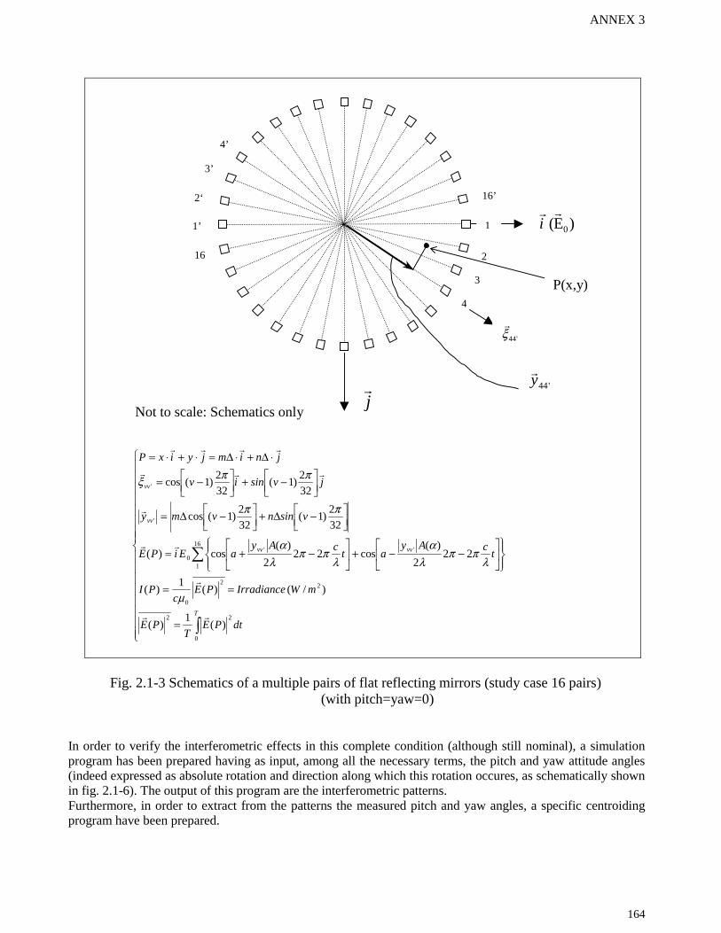
ANNEX 3

164

Not to scale: Schematics only

=

==

−−+

−+=

−∆+

−∆=

−+

−=

⋅∆+⋅∆=⋅+⋅=

T

vvvv

vv

vv

dtPET

PE

mWIrradiancePEc

PI

tcAy

atcAy

aEiPE

vsinnvmy

jvsiniv

jnimjyixP

0

22

22

0

16

1

''0

'

'

)(1

)(

)/( )(1

)(

222

)(cos22

2

)(cos)(

32

2)1(

32

2)1(cos

32

2)1(

32

2)1(cos

µ

λππ

λα

λππ

λα

ππ

ππξ

Fig. 2.1-3 Schematics of a multiple pairs of flat reflecting mirrors (study case 16 pairs)(with pitch=yaw=0)

In order to verify the interferometric effects in this complete condition (although still nominal), a simulationprogram has been prepared having as input, among all the necessary terms, the pitch and yaw attitude angles(indeed expressed as absolute rotation and direction along which this rotation occures, as schematically shownin fig. 2.1-6). The output of this program are the interferometric patterns.Furthermore, in order to extract from the patterns the measured pitch and yaw angles, a specific centroidingprogram have been prepared.

)E( 0

i

j

11’

2

2‘

3

3’

4

4’

16

16’

P(x,y)

'44ξ

'44y

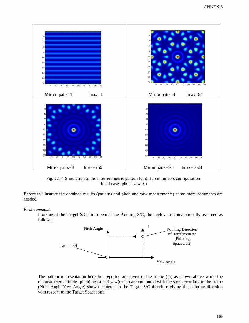
ANNEX 3

165

Mirror pairs=1 Imax=4 Mirror pairs=4 Imax=64

Mirror pairs=8 Imax=256 Mirror pairs=16 Imax=1024

Fig. 2.1-4 Simulation of the interferometric pattern for different mirrors configuration(in all cases pitch=yaw=0)

Before to illustrate the obtained results (patterns and pitch and yaw measurments) some more comments areneeded.

First comment.Looking at the Target S/C, from behind the Pointing S/C, the angles are conventionally assumed asfollows:

The pattern representation hereafter reported are given in the frame (i,j) as shown above while thereconstructed attitudes pitch(meas) and yaw(meas) are computed with the sign according to the frame(Pitch Angle,Yaw Angle) shown centered in the Target S/C therefore giving the pointing directionwith respect to the Target Spacecraft.

20 40 60 80 100 120 140 160 180 200

20

40

60

80

100

120

140

160

180

200 20 40 60 80 100 120 140 160 180 200

20

40

60

80

100

120

140

160

180

200

20 40 60 80 100 120 140 160 180 200

20

40

60

80

100

120

140

160

180

20020 40 60 80 100 120 140 160 180 200

20

40

60

80

100

120

140

160

180

200

Target S/C

Pointing Directionof Interferometer

(PointingSpacecraft)

Yaw Angle

Pitch Angle i

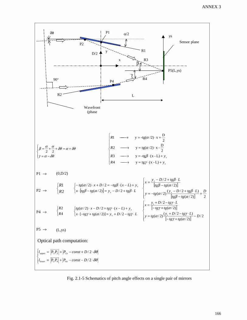
ANNEX 3

166

R4

R3

R2

R1D/2

P2

P1

P4

γ

β

90°

Sensor plane

δθ α/2

Wavefront(phase

L

ys

x

y

P5(L,ys)

−=

+=++=

δθαγ

δθαδθααβ22

+⋅=→

+⋅=→

⋅=→

+⋅=→

s

s

yR

yR

R

R

L)-x(tgy 4

L)-x(-tgy 3

2

D-x /2)tg(y 2

2

Dx /2)-tg(y 1

γβ

α

α

P1 → (0,D/2)

P2 →

2

1

R

R[ ]

⋅+−=−⋅+−⋅−=+⋅−

LtgDytgtgx

yLxtgDxtg

s

s

βαββα

2/)2/(

)(2/)2/( [ ]

[ ]

+−

⋅+−−=

−⋅+−

=

2)2/(

)2/()2/(

)2/(

2/

D

tgtg

LtgDytgy

tgtg

LtgDyx

s

s

αββα

αββ

P4 →

4

2

R

R

⋅−+=+−⋅+−⋅=−⋅

LtgDytgtgx

yLxtgDxtg

s

s

γαγγα

2/)]2/([

)(2/)2/( [ ]

[ ]

−+−

⋅−+=

+−⋅−+

=

2/)2/(

)2/()2/(

)2/(

2/

Dtgtg

LtgDytgy

tgtg

LtgDyx

s

s

αγγα

αγγ

P5 → (L,ys)

Optical path computation:

⋅−−+=

⋅+−+=

δθ

δθ

2/P

2/P

445

225

DconstPPl

DconstPPl

xlower

xupper

Fig. 2.1-5 Schematics of pitch angle effects on a single pair of mirrors

ANNEX 3

167

=

−⋅+

−⋅−=•=

−+

−−=

+=⋅=

'

32

2)1(cos

32

2)1(cos)(

32

2)1(cos

32

2)1()(

)cos(

'

'

vvpairtheaffectingRotation

vsinvsin

jvivsin

sinjin

aanvva

nvv

aaa

δθ

πψδθπψδθξθδδθ

ππξ

ψψδθδθθδ

Fig. 2.1-6 Effects of pitch and yaw rotations on all pairs of flat reflecting mirrors

Second comment.

With reference to the schematic reported in Fig.2.1-5, and to refelected rays phasing consideration, therelation between the ideal coordinates of the target spot in the sensor plane and the pitch and yawangles is given by (after all signs convention):

⋅⋅=

⋅⋅=

1803600) (cos

1803600) (cos

2

2

πα

πα

pitchLy

yawLx

s

s

where:L=Interferometer Length (m)ALFA= Interferometer aspect ratio (rad)Pitch= Pitch angle (arcsec)Xs, Ys = Ideal coordinates of the target spot in the sensor plane (m)

This allows to compute the pitch(meas) and yaw(meas) based on the Target spot coordinatesXs(meas) and Ys(meas), estimated by an appropriate centroiding algorithm.Furthermore above relations can be used for the definition of the ‘field of view’ that can be consideredas the max values of the pitch and yaw angles bringing the Target nominal spot in the sensor plane tothe sensor boarders.

Four reference cases have been investigated to have a first overview of the ‘nominal interferometer’behaviour. The results are summarized in fig. 2.1-7 and hereafter discussed.For all cases the following conditions were assumed:

λ= light wavelength= 0.0000005 (m)= 0.5 (µ)Interferometer Diameter = 0.3 (m)α= 0.03 (rad)DELTA= sensor discretisation= 0.0000005 (m)= 0.5 (µ)

j

ψ

θδ

ξ

)(ξ

ANNEX 3

168

Case # 1N=-/+ 70Total angle inclination (input) = 1.0300’’Direction ψ of inclination (input) = 70° True Pitch=0.9679’’ True Yaw=0.3523’’

Case # 2N=-/+ 20Total angle inclination (input) = 0.2350’’Direction ψ of inclination (input) = 135° True Pitch=0.16617’’ True Yaw=-0.16617’’

Case # 3N=-/+ 20Total angle inclination (input) = 0.0130’’Direction ψ of inclination (input) = 340° True Pitch=-0.004446’’

True Yaw=0.01222’’

Case # 4N=-/+ 20Total angle inclination (input) = 0.0020’’Direction ψ of inclination (input) = 250° True Pitch=-0.001879’’ True Yaw=-0.0006840’’

Shown F.O.V 2.9’’x 2.9’’True Attitude: Pitch=0.9679’’ Yaw=0.3523’’Measured Attitude: Pitch=0.9675’’ Yaw=0.3521’’Max. Power=1023.8 Attitude errors < 0.0004’’

Case # 1

Shown F.O.V. 0.84’’x 0.84’’True Attitude: Pitch=0.1662’’ Yaw=-0.1662’’Measured Attitude: Pitch=0.1661’’ Yaw=-0.1661’’Max. Power=1023.9 Attitude errors<0.0001’’

Case # 2

Shown F.O.V. 0.84’’x 0.84’’True Attitude: Pitch=-0.004446’’ Yaw=0.01222’’Measured Attitude: Pitch=-0.0043’’ Yaw=0.0125’’Max. Power=1020.1 Attitude errors<0.0003’’

Case # 3

Shown F.O.V. 0.84’’x 0.84’’True Attitude: Pitch=-0.001879’’ Yaw=-.0006840’’Measured Attitude: Pitch=-0.0018’’ Yaw=-0.00066388’’Max. Power=1023.8 Attitude errors<0.00008’’

Case # 4

Fig. 2.1-7 Summary of investigated cases with pitch and yaw inclinations

As can be seen in above nominal cases the accuracy in pitch and yaw reconstruction is very high and theresults achieved utilizes always the same centroiding algorithm.

20 40 60 80 100 120 140

20

40

60

80

100

120

140

5 10 15 20 25 30 35 40

5

10

15

20

25

30

35

40

5 10 15 20 25 30 35 40

5

10

15

20

25

30

35

40

5 10 15 20 25 30 35 40

5

10

15

20

25

30

35

40

ANNEX 3

169

3. EVALUATION OF PERFORMANCES

In this section the performances of the interferometric relative attitude sensor are evaluated with a realisticCCD detector. A ‘medium size’ interferometer equipped with an existing CCD sensor of good quality isconsidered and the effects of the following types of disturbances simulated:

CCD pixels finite dimensions; difference on Fresnel reflection coefficients as a function of the polarization direction of the beam

electric field ( with respect to the beam-normal to mirror plane); CCD dark currents inhomogeneities, photons shot noise, read out noise;

The medium size interferometer configuration considered for performances evaluation has the following maincharacteristics (see also Fig. 3-1):

two reflections are considered, the first at the entrance optics on a set of 16 pairs of flat ‘mirrors’and the second on an intermediate optics constituted by a secondary set of 16 pairs of flat mirrors;the second reflection is implemented for the sole reason of keeping limited the total interferometerlenght;

the CCD sensor is placed at the ‘focus’ which in this case occures at the front; the optical parameters are assumed to be:

ALFA=0.02 (rad)D=300 (mm)L≅7500 (mm) focal

the overall interferometer externally looks like a cylinder with a length of about 4000 (mm) and adiameter of about 400 (mm).

The interferometer F.O.V. (assuming the CCD below described) result in 211’’x 211’’

Reflectors (mirrors)The entrance ‘mirrors’ can be made simply by substrate optical material surfaces (e.g. sapphire refractionindex n=1.77 @ 0.55 µm) very flat and polished which sees the incoming beam at a very high incidence angle( in this case about 89.5°) while the secondary optics which sees the beam at a very low incidence angle(in thiscase about 0.5°) can be constituded by actual mirrors. The dimensions for the two types of mirrors are assumesas:

- entrance mirror: 20 (mm)x 1000(mm); the lenght can be reduced to e.g. 500 (mm) with a reductionin the FOV to 105’’x105’’ which is acceptable;

- secondary mirror: 12 (mm)x 12 (mm).Other types of optical substrate materials, with very low CTE, can be considered for space.

CCD detectors

The CCD considerd (Philips FT18) is operating in the visible range, in line with the laser source and ischaracterized by low pixel size compared to similar high quality products; the main features are the following:

- optical size: 7.68 (mm)x 7.68 (mm);- pixels number: 1024x1024;- pixel dimension: 7.5µm x 7.5µm;- conversion factor: 10 µV/el;- full well capacity: 45 kel/px (max voltage about 0.45V);- read out noise: 30 el;- shot noise: 10 el/px;- dark current: 1400 el/sec/px;- dark signal non uniformity (after compensation): 140 el/sec/px (estimated as 10% of dark current).

ANNEX 3

170

Interferometer schemetics (not to scale)

Front View Overall view (some mirror are not shown for viewing purposes)

Fig. 3-1 Medium size Interferometer configuration with single secondary reflection

Laser source

As far as the laser source, the following is assumed:- type: Melles Griot CW HeNe (05LHP927);- λ= 632.8 nm;- output power> 35 mW;- transversal mode: TEM00;- coherence lenght> 1 m (typical);- polarization: linear >500:1

Two reference cases are reported for the medium size study case:

Case 1:Total angle inclination (input) = 0.2025’’Direction ψ of inclination (input) = 20° this means:

True Pitch=0.06926’’ True Yaw=0.19029’’

Case 2:Total angle inclination (input) = 0.00136’’Direction ψ of inclination (input) = 95° this means:

True Pitch=0.001355’’ True Yaw=-0.0001185’’

Starting from the results achieved in nominal conditions with no disturbance sources and pixels very small(Cases 1N and 2N shown in Fig. 3-2) three types of analysis have been performed for each of the cases:

Entrance Optic# 32 flat skewed mirrors

Detector

Secondary Optics

Entrance Beam

D=300 mm

L=4000 mm

ANNEX 3

171

- Finite pixel dimensions effects (Cases 1N1 and 2N1 in Fig. 3-3);- Finite pixel dimensions effects and reflection coefficients mismatch (Cases 1N2 and 2N2, Fig. 3-5);- Finite pixel dimensions effects and reflection coefficients mismatch and CCD photoelectrical

disturbances (reported in Tab. 3-1).

Fig 3-4 summarizes the main relations of Fresnel reflection.To include the CCD electrooptical features the logical steps followed have been:

- computation of the energy per pixel gathered in a specified exposure time (taking into accountpixel size and reflection coefficient mismatch);

- computation of the electrons per pixel generated by the signal;- perturbation of the electron number by the disturbances of dark currents inhomogeneities, photons

shot noise and read out noise;- computation of the CCD output voltage map and centroiding for pitch and yaw estimation.

Shown F.O.V. 1.11’’x 1.11’’True Attitude: Pitch=0.06926’’ Yaw=0.19029’’Measured Attitude: Pitch=0.0692’’ Yaw=0.1903’’Max. Power=1023.9 Attitude errors<0.0001’’Case # 1N

Shown F.O.V. 0.83’’x 0.83’’True Attitude: Pitch=0.001355’’ Yaw=-0.0001185’’Measured Attitude: Pitch=0.0013’’ Yaw=-0.0001174’’Max. Power=1024.0 Attitude errors<0.0001’’Case # 2N

Fig. 3-2 Nominal reference cases

Shown F.O.V. 6.4’’x 6.4’’Pixel size=7.5µmTrue Attitude: Pitch=0.06926’’ Yaw=0.19029’’Measured Attitude: Pitch=0.0699’’ Yaw=0.1892’’Max. Power=895.6 Attitude errors=0.001’’Case # 1N1

Shown F.O.V. 6.4’’x 6.4’’Pixel size=7.5µmTrue Attitude: Pitch=0.001355’’ Yaw=-0.0001185’’Measured Attitude: Pitch=0.0015’’ Yaw=-0.000127’’Max. Power=1024.0 Attitude errors<0.0002’’Case # 2N1

Fig. 3-3 Effects of pixel finite dimensions on the two Nominal reference cases

10 20 30 40 50 60 70 80

10

20

30

40

50

60

70

8010 20 30 40 50 60

10

20

30

40

50

60

5 10 15 20 25 30

5

10

15

20

25

30

5 10 15 20 25 30

5

10

15

20

25

30

ANNEX 3

172

Fig. 3-4 Schematics for the reflection coefficients

Shown F.O.V. 6.4’’x 6.4’’Pixel size=7.5µmRefl. Mismatch=2.9%True Attitude: Pitch=0.06926’’ Yaw=0.19029’’Measured Attitude: Pitch=0.0698’’ Yaw=0.1892’’Max. Power=929.6 Attitude errors=0.001’’Case # 1N2

Shown F.O.V. 6.4’’x 6.4’’Pixel size=7.5µmRefl. Mismatch=2.9%True Attitude: Pitch=0.001355’’ Yaw=-0.0001185’’Measured Attitude: Pitch=0.0015’’ Yaw=-0.000127’’Max. Power=1062 Attitude errors<0.0002’’Case # 2N2

Fig. 3-5 Effects of reflection coefficients mismatch and of pixel finite dimensions

Furthermore the follwing remarks are noted:- the irradiance (W/m^2) at the entrance of the interferometer is computed considering a 35 mW

laser with beam divergence controlled at 5 arcsec. The irradiance at the interferometer will resultof at least 0.000001 (W/m^2) assuming a target/interferometer distance of 10000 km;

- the exposure time should be high enough to collect a number of electrons from the signalsufficient to duly exceed the shot and read out electrons (which constitute a socket);

- the dark current inhomogeneities represent the residual errors of the dark currents after theircompensation; the inhomogeneities integrate with time as the number of photons/electrons of thesignal.

5 10 15 20 25 30

5

10

15

20

25

30

5 10 15 20 25 30

5

10

15

20

25

30

ANNEX 3

173

Case 1N2 (update rate of 10 Hz and 35 mW laser)True Pitch=0.06926’’True Yaw=0.19029’’ Frequency update rate [Hz]:10Number of row :31Number of columns :31Number of cases for statistics :100pitch error rms (arcsec) = 0.0096pitch average (arcsec) = 0.0609yaw error rms (arcsec) = 0.0043yaw average (arcsec) = 0.1904

Case 1N2 (update rate of 2 Hz and 35 mW laser)True Pitch=0.06926’’True Yaw=0.19029’’Frequency update rate [Hz]:2Number of row :31Number of columns :31Number of cases for statistics :100pitch error rms (arcsec) = 0.0033pitch average (arcsec) = 0.0664yaw error rms (arcsec) = 0.0019

yaw average (arcsec) = 0.1897

Case 2N2 (update rate of 10 Hz and 35 mW laser)True Pitch=0.001355’’True Yaw=-0.0001185’’Reflection coefficients :0.958Frequency update rate [Hz]:10Number of row :31Number of columns :31Number of cases for statistics :100pitch error rms (arcsec) = 0.0044pitch average (arcsec) = 0.0018yaw error rms (arcsec )= 0.0041yaw average (arcsec) = -8.0759e-004

Case 2N2 ( update rate of 2 Hz and 35 mW laser)True Pitch=0.001355’’True Yaw=-0.0001185’’Reflection coefficients :0.958Frequency update rate [Hz]:2Number of row :31Number of columns :31Number of cases for statistics :100pitch error rms (arcsec) = 0.0017pitch average (arcsec) = 0.0016yaw error rms (arcsec) = 0.0016yaw average (arcsec) = -5.1987e-004

Tab. 3-1 Performances including all disturbances for the two reference cases and at twoacquisition frequencies (for the discussed interferometer)

4. GENERAL REMARKS

Relative attitude sensors based on wavefront splitting interferometry constitute a very promisingtechnique for the future missions involving two or more Spacecrafts to be relatively controlled. Thetechnique here presented utilizes flat mirrors only which in principle can be manufactured withextreme flatness.This characteristics, in conjunction with the ever increasing CCD technology and in combinationwith high efficiency centroiding algorithms, allows for very precise relative attitude determination.Of course the final performances of these interferometer systems will depend on other parameters ofwhich of primary importance are the dimensional stability against changing envioronmentalconditions as well as deformation following launch. To exploit full performances it will be necessaryto implement an internal metrology system in a manner similar to multitelescope techniques forastrometric missions.Depending on the specific mission/scientific needs, Space Platforms forming the future constellationscan be relatively aligned with great accuracy thus opening to impressive scientific and experimentalpossibilities.