Dipartimento di Elettronica e Telecomunicazioni ... · Politecnico di Torino - DET M. Taragna • A...
67
SYSTEM IDENTIFICATION Michele TARAGNA Dipartimento di Elettronica e Telecomunicazioni Politecnico di Torino [email protected] Master Course in Mechatronic Engineering Master Course in Computer Engineering 01RKYQW / 01RKYOV “Estimation, Filtering and System Identification” Academic Year 2019/2020
Transcript of Dipartimento di Elettronica e Telecomunicazioni ... · Politecnico di Torino - DET M. Taragna • A...

SYSTEM IDENTIFICATION
Michele TARAGNA
Dipartimento di Elettronica e Telecomunicazioni
Politecnico di Torino
Master Course in Mechatronic Engineering
Master Course in Computer Engineering
01RKYQW / 01RKYOV “Estimation, Filtering and System Identi fication”
Academic Year 2019/2020
Politecnico di Torino - DET M. Taragna
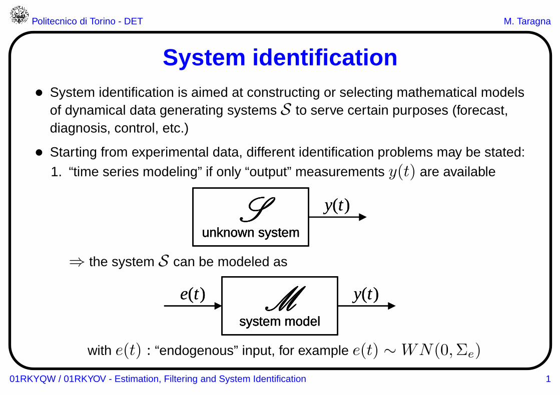
System identification• System identification is aimed at constructing or selecting mathematical models
of dynamical data generating systems S to serve certain purposes (forecast,diagnosis, control, etc.)
• Starting from experimental data, different identification problems may be stated:
1. “time series modeling” if only “output” measurements y(t) are available
unknown systemS y(t)
unknown systemS
unknown systemS
unknown systemS y(t)
⇒ the system S can be modeled as
e(t)
system modelM y(t)e(t)
system modelM
system modelM
system modelM y(t)
with e(t) : “endogenous” input, for example e(t) ∼WN(0,Σe)
01RKYQW / 01RKYOV - Estimation, Filtering and System Identification 1
Politecnico di Torino - DET M. Taragna
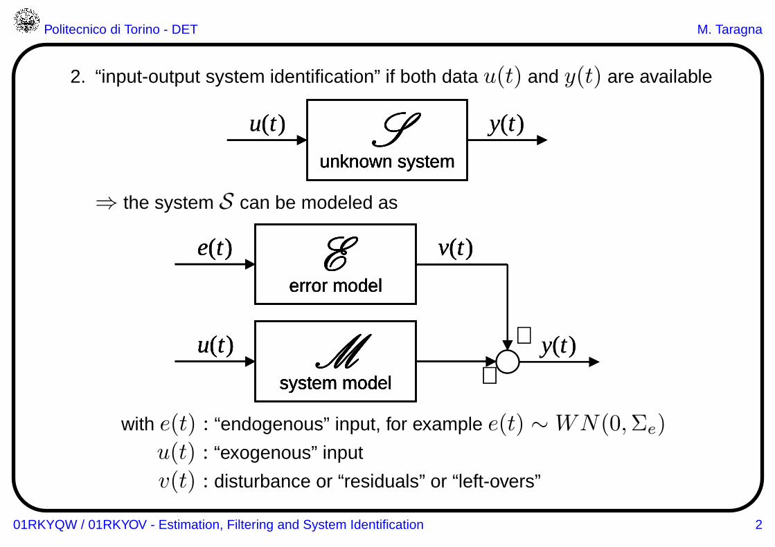
2. “input-output system identification” if both data u(t) and y(t) are available
u(t)
unknown systemS y(t)u(t)
unknown systemS
unknown systemS
unknown systemS y(t)
⇒ the system S can be modeled as
e(t)
error modelE v(t)
u(t)
system modelM
+
+y(t)
e(t)
error modelE v(t)e(t)
error modelE
error modelE
error modelE v(t)
u(t)
system modelMu(t)
system modelM
system modelM
system modelM
+
+y(t)
with e(t) : “endogenous” input, for example e(t) ∼WN(0,Σe)
u(t) : “exogenous” input
v(t) : disturbance or “residuals” or “left-overs”
01RKYQW / 01RKYOV - Estimation, Filtering and System Identification 2
Politecnico di Torino - DET M. Taragna
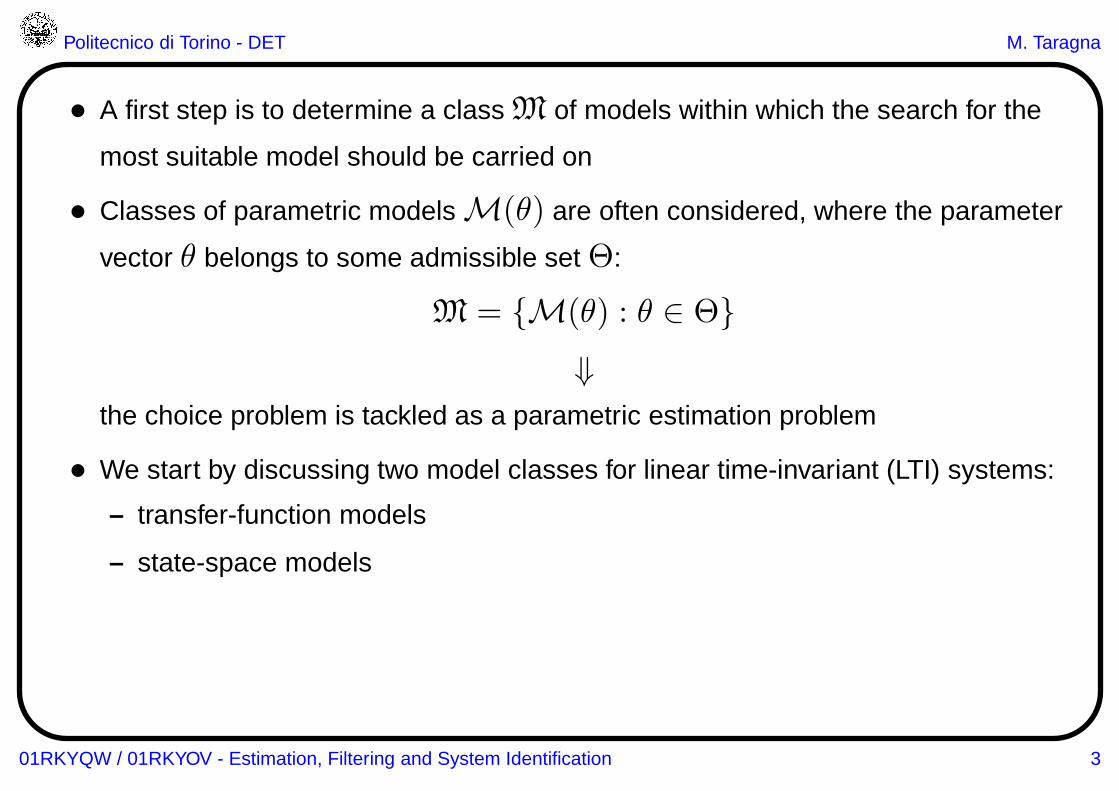
• A first step is to determine a class M of models within which the search for the
most suitable model should be carried on
• Classes of parametric models M(θ) are often considered, where the parameter
vector θ belongs to some admissible set Θ:
M = {M(θ) : θ ∈ Θ}⇓
the choice problem is tackled as a parametric estimation problem
• We start by discussing two model classes for linear time-invariant (LTI) systems:
– transfer-function models
– state-space models
01RKYQW / 01RKYOV - Estimation, Filtering and System Identification 3
Politecnico di Torino - DET M. Taragna
Transfer-function models
• The transfer-function models, known also as black-box or Box-Jenkins models,
involve external variables only (i.e., input and output variables) and do not require
any auxiliary variable
• Different structures of transfer-function models are available:
– equation error or ARX model structure
– ARMAX model structure
– output error (OE) model structure
– Box-Jenkins (BJ) model structure
01RKYQW / 01RKYOV - Estimation, Filtering and System Identification 4
Politecnico di Torino - DET M. Taragna
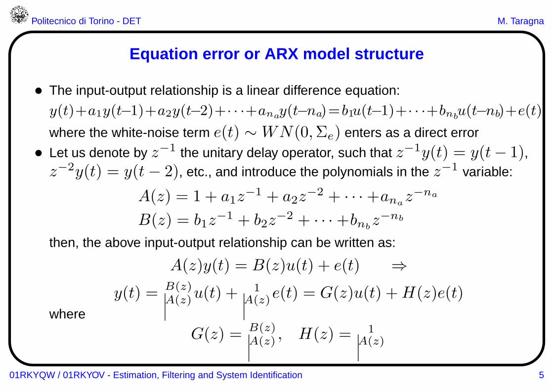
Equation error or ARX model structure
• The input-output relationship is a linear difference equation:
y(t)+a1y(t−1)+a2y(t−2)+· · ·+anay(t−na)=b1u(t−1)+· · ·+bnbu(t−nb)+e(t)
where the white-noise term e(t) ∼WN(0,Σe) enters as a direct error
• Let us denote by z−1 the unitary delay operator, such that z−1y(t) = y(t− 1),z−2y(t) = y(t− 2), etc., and introduce the polynomials in the z−1 variable:
A(z) = 1 + a1z−1 + a2z
−2 + · · ·+anaz−na
B(z) = b1z−1 + b2z
−2 + · · ·+bnbz−nb
then, the above input-output relationship can be written as:
A(z)y(t) = B(z)u(t) + e(t) ⇒y(t) = B(z)
A(z)u(t) +1
A(z)e(t) = G(z)u(t) +H(z)e(t)
where
G(z) = B(z)A(z) , H(z) = 1
A(z)
01RKYQW / 01RKYOV - Estimation, Filtering and System Identification 5
Politecnico di Torino - DET M. Taragna
+
+y(t)
e(t) v(t)H(z)=
A(z)1
u(t)G(z)=
A(z)B(z) +
+y(t)
e(t) v(t)H(z)=
A(z)1e(t) v(t)
H(z)=A(z)
1H(z)=
A(z)1
H(z)=A(z)
1A(z)
1
u(t)G(z)=
A(z)B(z)u(t)
G(z)=A(z)B(z)
G(z)=A(z)B(z)
G(z)=A(z)B(z)A(z)B(z)
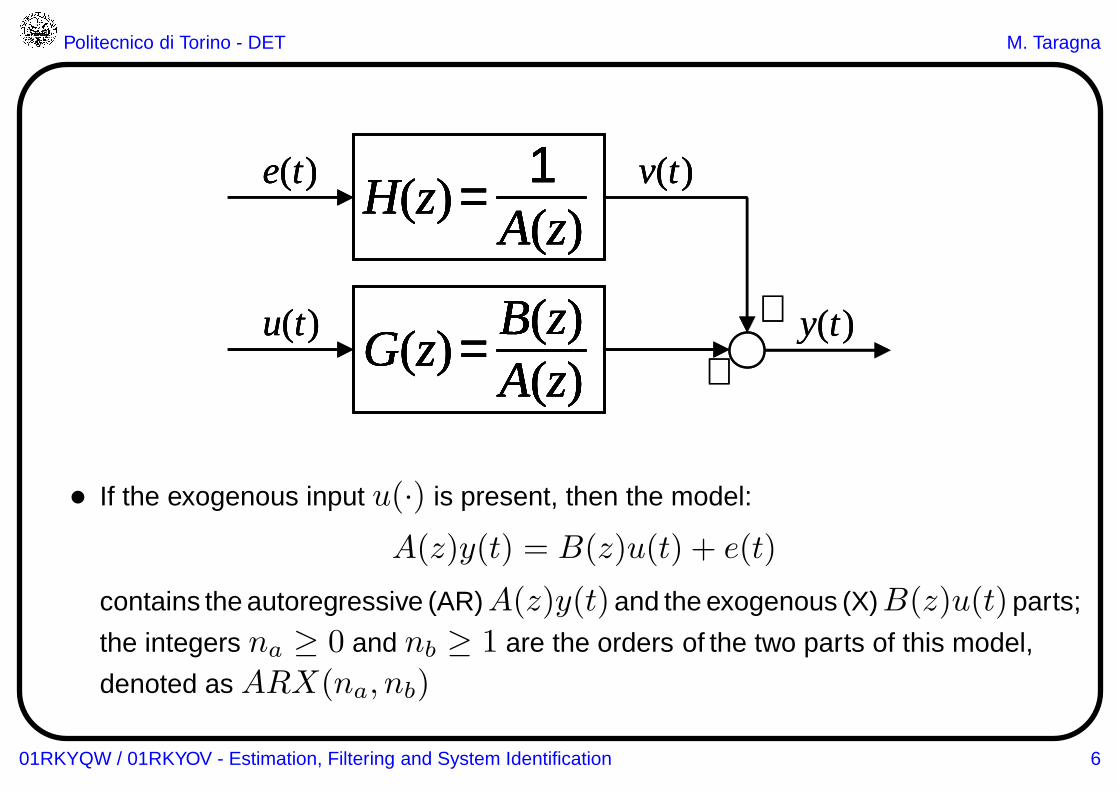
• If the exogenous input u(·) is present, then the model:
A(z)y(t) = B(z)u(t) + e(t)
contains the autoregressive (AR)A(z)y(t)and the exogenous (X)B(z)u(t)parts;
the integers na ≥ 0 and nb ≥ 1 are the orders of the two parts of this model,
denoted as ARX(na, nb)
01RKYQW / 01RKYOV - Estimation, Filtering and System Identification 6
Politecnico di Torino - DET M. Taragna
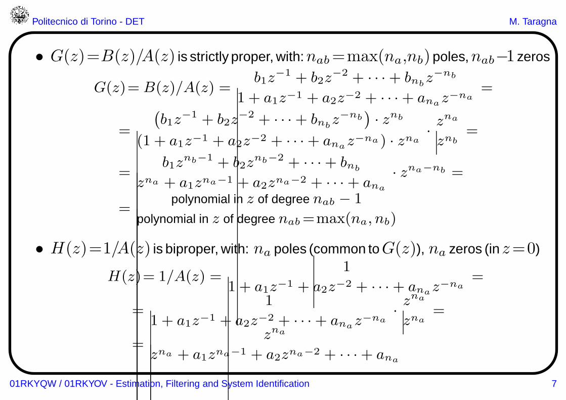
• G(z)=B(z)/A(z) is strictly proper, with:nab=max(na,nb)poles,nab−1 zeros
G(z)= B(z)/A(z) =b1z
−1 + b2z−2 + · · ·+ bnb
z−nb
1 + a1z−1 + a2z−2 + · · ·+ anaz−na
=
=
(
b1z−1 + b2z
−2 + · · ·+ bnbz−nb
)
· znb
(1 + a1z−1 + a2z−2 + · · ·+ anaz−na) · zna
·zna
znb=
=b1z
nb−1 + b2znb−2 + · · ·+ bnb
zna + a1zna−1 + a2zna−2 + · · ·+ ana
· zna−nb =
=polynomial in z of degree nab − 1
polynomial in z of degree nab=max(na, nb)
• H(z)=1/A(z) is biproper, with: na poles (common toG(z)), na zeros (inz=0)
H(z)= 1/A(z) =1
1 + a1z−1 + a2z−2 + · · ·+ anaz−na
=
=1
1 + a1z−1 + a2z−2 + · · ·+ anaz−na
·zna
zna=
=zna
zna + a1zna−1 + a2zna−2 + · · ·+ ana
01RKYQW / 01RKYOV - Estimation, Filtering and System Identification 7
Politecnico di Torino - DET M. Taragna
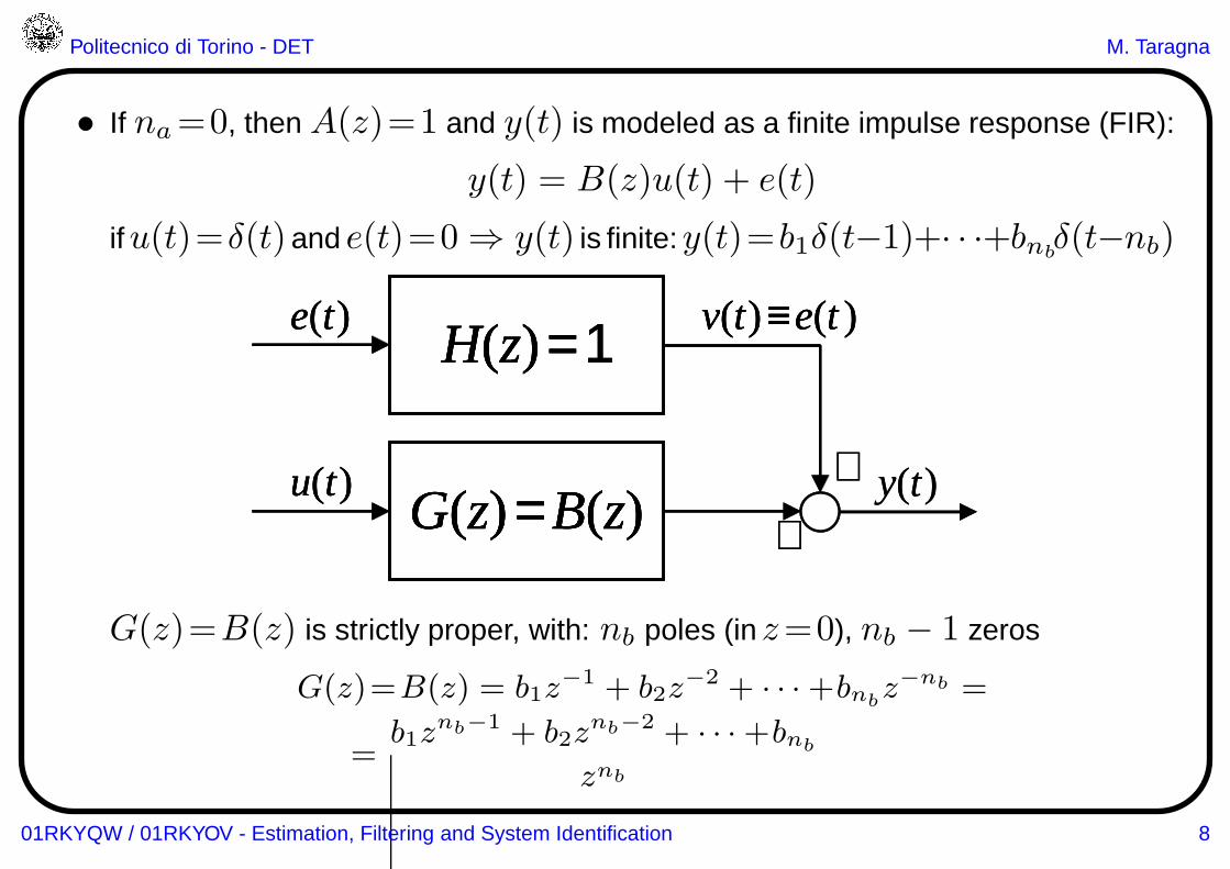
• If na=0, then A(z)=1 and y(t) is modeled as a finite impulse response (FIR):
y(t) = B(z)u(t) + e(t)
ifu(t)=δ(t)and e(t)=0 ⇒ y(t) is finite:y(t)=b1δ(t−1)+· · ·+bnbδ(t−nb)
+
+y(t)
e(t) v(t)≡ e(t )H(z)= 1
u(t)G(z) = B(z)
+
+y(t)
e(t) v(t)≡ e(t )H(z)= 1e(t) v(t)≡ e(t )H(z)= 1H(z)= 1
u(t)G(z) = B(z)
u(t)G(z) = B(z)G(z) = B(z)
G(z)=B(z) is strictly proper, with: nb poles (inz=0), nb − 1 zeros
G(z)=B(z) = b1z−1 + b2z
−2 + · · ·+bnbz−nb =
=b1z
nb−1 + b2znb−2 + · · ·+bnb
znb
01RKYQW / 01RKYOV - Estimation, Filtering and System Identification 8
Politecnico di Torino - DET M. Taragna
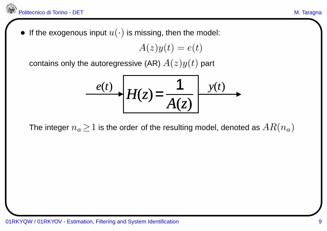
• If the exogenous input u(·) is missing, then the model:
A(z)y(t) = e(t)
contains only the autoregressive (AR) A(z)y(t) part
e(t) y(t)H(z) =
A(z)1e(t) y(t)
H(z) =A(z)
1H(z) =
A(z)1
H(z) =A(z)
1A(z)
1
The integer na≥1 is the order of the resulting model, denoted as AR(na)
01RKYQW / 01RKYOV - Estimation, Filtering and System Identification 9
Politecnico di Torino - DET M. Taragna
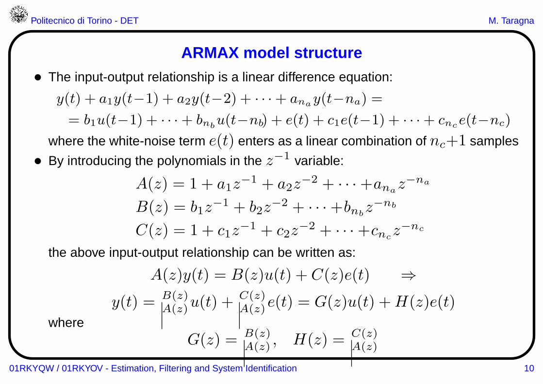
ARMAX model structure• The input-output relationship is a linear difference equation:
y(t) + a1y(t−1) + a2y(t−2) + · · ·+ anay(t−na) =
= b1u(t−1) + · · ·+ bnbu(t−nb) + e(t) + c1e(t−1) + · · ·+ cnce(t−nc)
where the white-noise term e(t) enters as a linear combination of nc+1 samples
• By introducing the polynomials in the z−1 variable:
A(z) = 1 + a1z−1 + a2z
−2 + · · ·+anaz−na
B(z) = b1z−1 + b2z
−2 + · · ·+bnbz−nb
C(z) = 1 + c1z−1 + c2z
−2 + · · ·+cncz−nc
the above input-output relationship can be written as:
A(z)y(t) = B(z)u(t) + C(z)e(t) ⇒y(t) = B(z)
A(z)u(t) +C(z)A(z)e(t) = G(z)u(t) +H(z)e(t)
whereG(z) = B(z)
A(z) , H(z) = C(z)A(z)
01RKYQW / 01RKYOV - Estimation, Filtering and System Identification 10
Politecnico di Torino - DET M. Taragna
+
+y(t)
e(t) v(t)H(z)=
A(z)C(z)
u(t)G(z)=
A(z)B(z) +
+y(t)
e(t) v(t)H(z)=
A(z)C(z)e(t) v(t)
H(z)=A(z)C(z)
H(z)=A(z)C(z)
H(z)=A(z)C(z)A(z)C(z)
u(t)G(z)=
A(z)B(z)u(t)
G(z)=A(z)B(z)
G(z)=A(z)B(z)
G(z)=A(z)B(z)A(z)B(z)
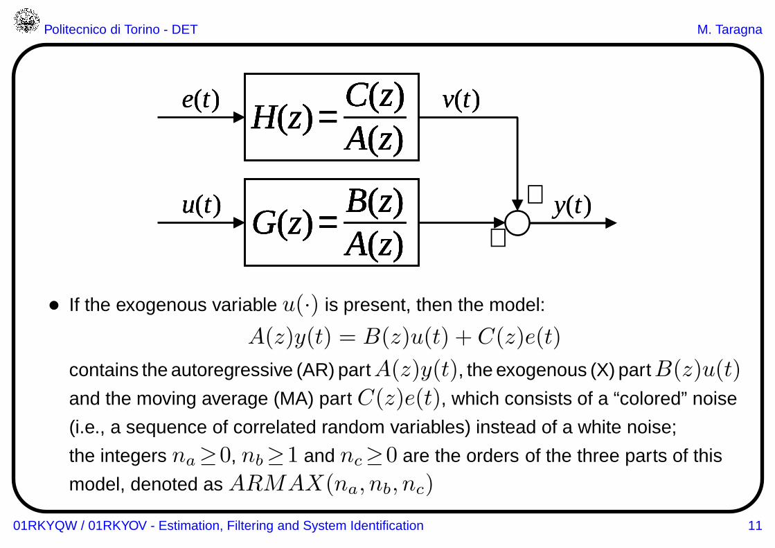
• If the exogenous variable u(·) is present, then the model:
A(z)y(t) = B(z)u(t) + C(z)e(t)
contains the autoregressive (AR) partA(z)y(t), the exogenous (X) partB(z)u(t)
and the moving average (MA) part C(z)e(t), which consists of a “colored” noise
(i.e., a sequence of correlated random variables) instead of a white noise;
the integers na≥0, nb≥1 and nc≥0 are the orders of the three parts of this
model, denoted as ARMAX(na, nb, nc)
01RKYQW / 01RKYOV - Estimation, Filtering and System Identification 11

Politecnico di Torino - DET M. Taragna
• G(z)=B(z)/A(z) is strictly proper, with:nab=max(na,nb)poles,nab−1 zeros
• H(z)=C(z)/A(z) is biproper, with: nac=max(na,nc)poles, nac zeros
H(z)= C(z)/A(z) =1 + c1z
−1 + c2z−2 + · · ·+ cncz
−nc
1 + a1z−1 + a2z−2 + · · ·+ anaz−na
=
=
(
1 + c1z−1 + c2z
−2 + · · ·+ cncz−nc
)
· znc
(1 + a1z−1 + a2z−2 + · · ·+ anaz−na) · zna
·zna
znc=
=znc + c1z
nc−1 + c2znc−2 + · · ·+ cnc
zna + a1zna−1 + a2zna−2 + · · ·+ ana
· zna−nc =
=polynomial in z of degree nac=max(na, nc)
polynomial in z of degree nac
The na roots of the polynomial A(z) are common poles to G(z) and H(z)
01RKYQW / 01RKYOV - Estimation, Filtering and System Identification 12
Politecnico di Torino - DET M. Taragna
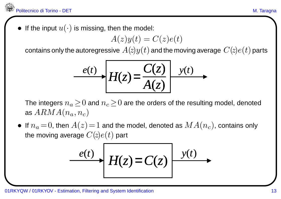
• If the input u(·) is missing, then the model:
A(z)y(t) = C(z)e(t)
contains only the autoregressive A(z)y(t)and the moving average C(z)e(t)parts
e(t) y(t)H(z) =
A(z)C(z)e(t) y(t)
H(z) =A(z)C(z)
H(z) =A(z)C(z)
H(z) =A(z)C(z)A(z)C(z)
The integers na≥0 and nc≥0 are the orders of the resulting model, denotedas ARMA(na, nc)
• If na=0, then A(z)=1 and the model, denoted as MA(nc), contains onlythe moving average C(z)e(t) part
e(t) y(t)H(z) = C(z)
e(t) y(t)H(z) = C(z)H(z) = C(z)
01RKYQW / 01RKYOV - Estimation, Filtering and System Identification 13
Politecnico di Torino - DET M. Taragna
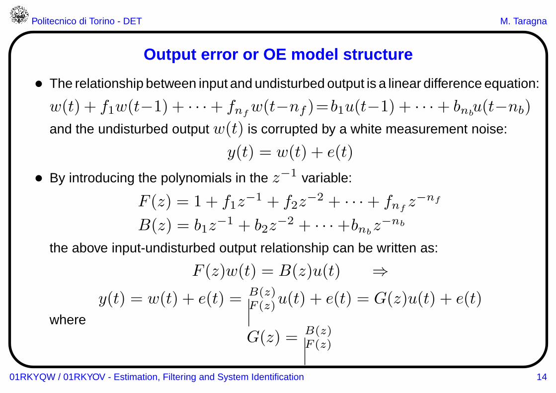
Output error or OE model structure
• The relationship between input and undisturbed output is a linear difference equation:
w(t) + f1w(t−1) + · · ·+ fnfw(t−nf )=b1u(t−1) + · · ·+ bnb
u(t−nb)
and the undisturbed output w(t) is corrupted by a white measurement noise:
y(t) = w(t) + e(t)
• By introducing the polynomials in the z−1 variable:
F (z) = 1 + f1z−1 + f2z
−2 + · · ·+ fnfz−nf
B(z) = b1z−1 + b2z
−2 + · · ·+bnbz−nb
the above input-undisturbed output relationship can be written as:
F (z)w(t) = B(z)u(t) ⇒y(t) = w(t) + e(t) = B(z)
F (z)u(t) + e(t) = G(z)u(t) + e(t)
whereG(z) = B(z)
F (z)
01RKYQW / 01RKYOV - Estimation, Filtering and System Identification 14
Politecnico di Torino - DET M. Taragna
+
+y(t)
e(t) v(t)≡ e(t )H(z)= 1
u(t)G(z)=
F(z)B(z) w(t) +
+y(t)
e(t) v(t)≡ e(t )H(z)= 1e(t) v(t)≡ e(t )H(z)= 1H(z)= 1
u(t)G(z)=
F(z)B(z) w(t)u(t)
G(z)=F(z)B(z)
G(z)=F(z)B(z)
G(z)=F(z)B(z)F(z)B(z) w(t)
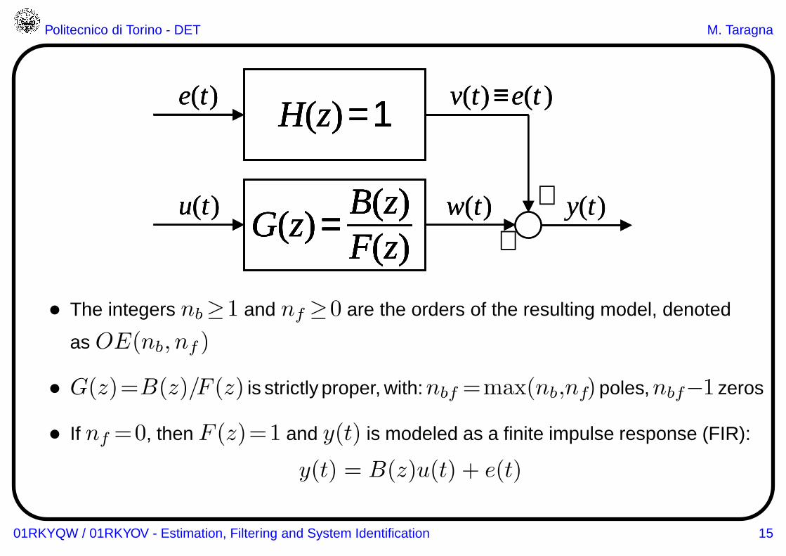
• The integers nb≥1 and nf ≥0 are the orders of the resulting model, denoted
as OE(nb, nf )
• G(z)=B(z)/F (z) is strictly proper, with:nbf =max(nb,nf)poles,nbf−1 zeros
• If nf =0, then F (z)=1 and y(t) is modeled as a finite impulse response (FIR):
y(t) = B(z)u(t) + e(t)
01RKYQW / 01RKYOV - Estimation, Filtering and System Identification 15
Politecnico di Torino - DET M. Taragna
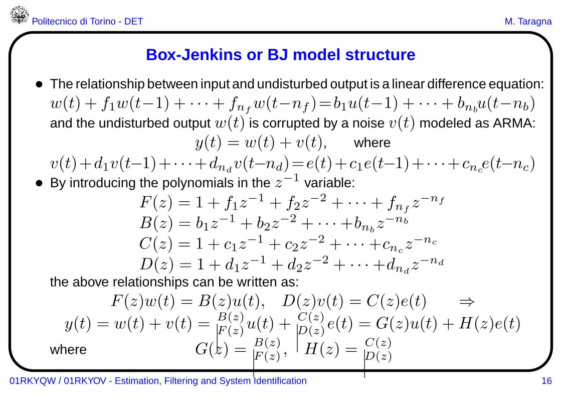
Box-Jenkins or BJ model structure
• The relationship between input and undisturbed output is a linear difference equation:w(t) + f1w(t−1) + · · ·+ fnf
w(t−nf )=b1u(t−1) + · · ·+ bnbu(t−nb)
and the undisturbed output w(t) is corrupted by a noise v(t) modeled as ARMA:y(t) = w(t) + v(t), where
v(t)+d1v(t−1)+ · · ·+dndv(t−nd)=e(t)+c1e(t−1)+ · · ·+cnc
e(t−nc)• By introducing the polynomials in the z−1 variable:
F (z) = 1 + f1z−1 + f2z
−2 + · · ·+ fnfz−nf
B(z) = b1z−1 + b2z
−2 + · · ·+bnbz−nb
C(z) = 1 + c1z−1 + c2z
−2 + · · ·+cncz−nc
D(z) = 1 + d1z−1 + d2z
−2 + · · ·+dndz−nd
the above relationships can be written as:F (z)w(t) = B(z)u(t), D(z)v(t) = C(z)e(t) ⇒
y(t) = w(t) + v(t) = B(z)F (z)u(t) +
C(z)D(z)e(t) = G(z)u(t) +H(z)e(t)
where G(z) = B(z)F (z) , H(z) = C(z)
D(z)
01RKYQW / 01RKYOV - Estimation, Filtering and System Identification 16
Politecnico di Torino - DET M. Taragna
+
+y(t)
e(t) v(t)H(z)=
D(z)C(z)
u(t)G(z)=
F(z)B(z) w(t) +
+y(t)
e(t) v(t)H(z)=
D(z)C(z)e(t) v(t)
H(z)=D(z)C(z)
H(z)=D(z)C(z)
H(z)=D(z)C(z)D(z)C(z)
u(t)G(z)=
F(z)B(z) w(t)u(t)
G(z)=F(z)B(z)
G(z)=F(z)B(z)
G(z)=F(z)B(z)F(z)B(z) w(t)
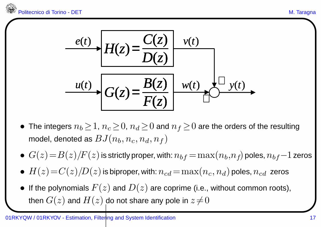
• The integers nb≥1, nc≥0, nd≥0 and nf ≥0 are the orders of the resulting
model, denoted as BJ(nb, nc, nd, nf )
• G(z)=B(z)/F (z) is strictly proper, with:nbf =max(nb,nf)poles,nbf−1 zeros
• H(z)=C(z)/D(z) is biproper, with:ncd=max(nc, nd)poles,ncd zeros
• If the polynomials F (z) and D(z) are coprime (i.e., without common roots),
then G(z) and H(z) do not share any pole in z 6=0
01RKYQW / 01RKYOV - Estimation, Filtering and System Identification 17
Politecnico di Torino - DET M. Taragna
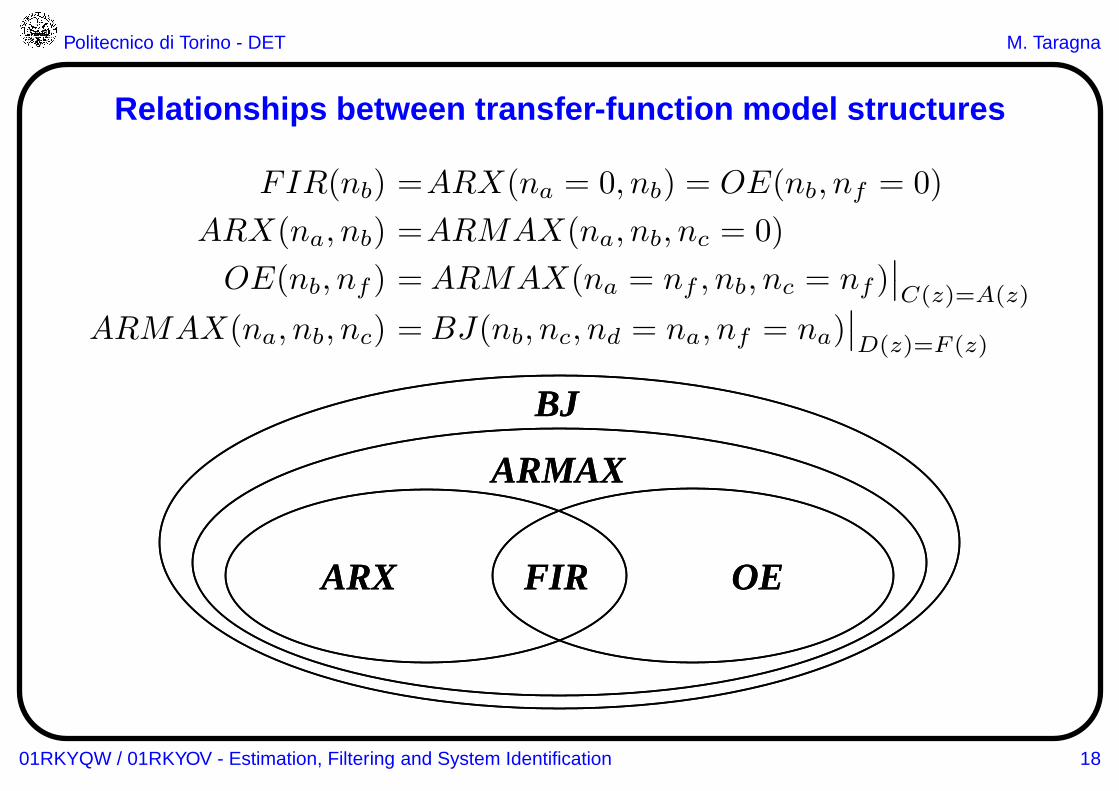
Relationships between transfer-function model structure s
FIR(nb) =ARX(na = 0, nb) = OE(nb, nf = 0)
ARX(na, nb) =ARMAX(na, nb, nc = 0)
OE(nb, nf ) = ARMAX(na = nf , nb, nc = nf )∣∣C(z)=A(z)
ARMAX(na, nb, nc) = BJ(nb, nc, nd = na, nf = na)∣∣D(z)=F (z)
FIR OEARX
ARMAX
BJ
FIR OEARX
ARMAX
BJ
01RKYQW / 01RKYOV - Estimation, Filtering and System Identification 18
Politecnico di Torino - DET M. Taragna
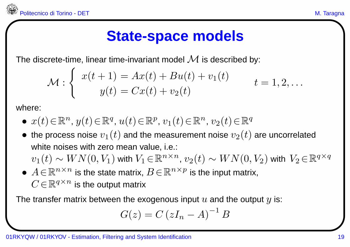
State-space modelsThe discrete-time, linear time-invariant model M is described by:
M :
{
x(t+ 1) = Ax(t) +Bu(t) + v1(t)
y(t) = Cx(t) + v2(t)t = 1, 2, . . .
where:
• x(t)∈Rn, y(t)∈R
q , u(t)∈Rp, v1(t)∈R
n, v2(t)∈Rq
• the process noise v1(t) and the measurement noise v2(t) are uncorrelatedwhite noises with zero mean value, i.e.:v1(t) ∼WN(0, V1) with V1∈R
n×n, v2(t) ∼WN(0, V2) with V2∈Rq×q
• A∈Rn×n is the state matrix, B∈R
n×p is the input matrix,C∈R
q×n is the output matrix
The transfer matrix between the exogenous input u and the output y is:
G(z) = C (zIn −A)−1B
01RKYQW / 01RKYOV - Estimation, Filtering and System Identification 19
Politecnico di Torino - DET M. Taragna
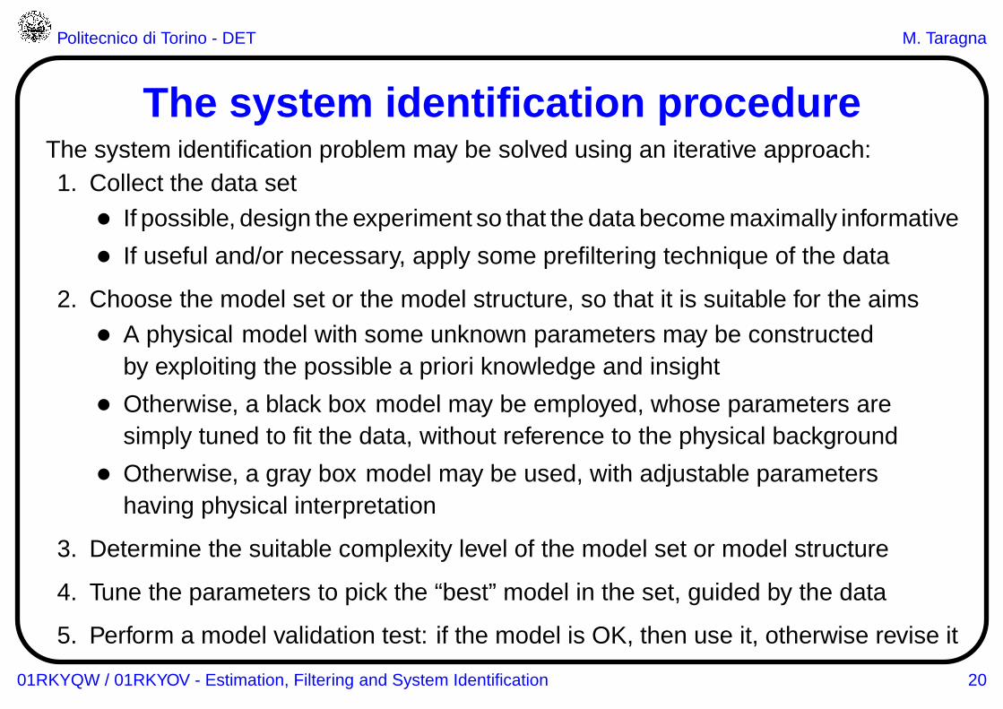
The system identification procedureThe system identification problem may be solved using an iterative approach:1. Collect the data set
• If possible, design the experiment so that the data become maximally informative
• If useful and/or necessary, apply some prefiltering technique of the data
2. Choose the model set or the model structure, so that it is suitable for the aims
• A physical model with some unknown parameters may be constructedby exploiting the possible a priori knowledge and insight
• Otherwise, a black box model may be employed, whose parameters aresimply tuned to fit the data, without reference to the physical background
• Otherwise, a gray box model may be used, with adjustable parametershaving physical interpretation
3. Determine the suitable complexity level of the model set or model structure
4. Tune the parameters to pick the “best” model in the set, guided by the data
5. Perform a model validation test: if the model is OK, then use it, otherwise revise it
01RKYQW / 01RKYOV - Estimation, Filtering and System Identification 20
Politecnico di Torino - DET M. Taragna
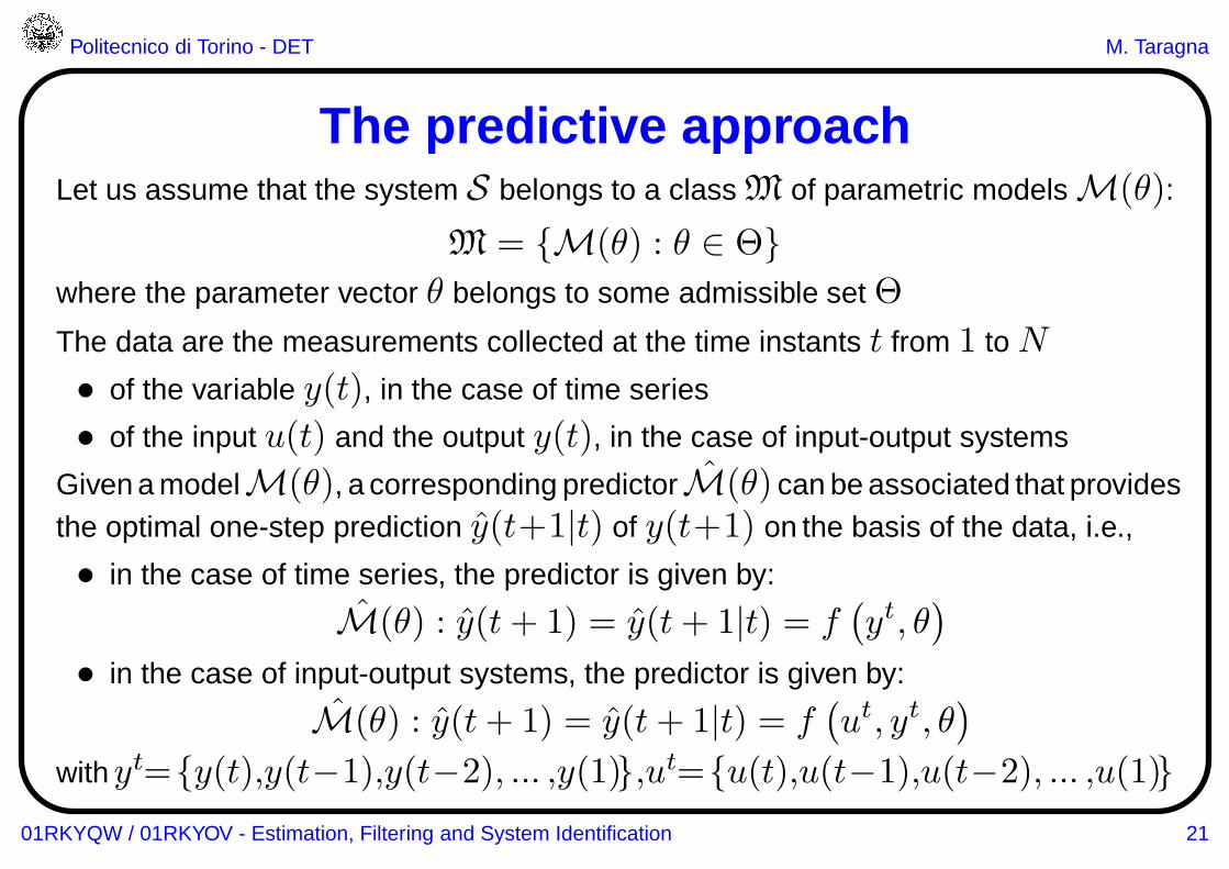
The predictive approachLet us assume that the system S belongs to a class M of parametric models M(θ):
M = {M(θ) : θ ∈ Θ}where the parameter vector θ belongs to some admissible set Θ
The data are the measurements collected at the time instants t from 1 to N
• of the variable y(t), in the case of time series
• of the input u(t) and the output y(t), in the case of input-output systems
Given a modelM(θ), a corresponding predictorM(θ) can be associated that providesthe optimal one-step prediction y(t+1|t) of y(t+1) on the basis of the data, i.e.,
• in the case of time series, the predictor is given by:
M(θ) : y(t+ 1) = y(t+ 1|t) = f(yt, θ
)
• in the case of input-output systems, the predictor is given by:
M(θ) : y(t+ 1) = y(t+ 1|t) = f(ut, yt, θ
)
withyt={y(t),y(t−1),y(t−2), ... ,y(1)},ut={u(t),u(t−1),u(t−2), ... ,u(1)}01RKYQW / 01RKYOV - Estimation, Filtering and System Identification 21
Politecnico di Torino - DET M. Taragna
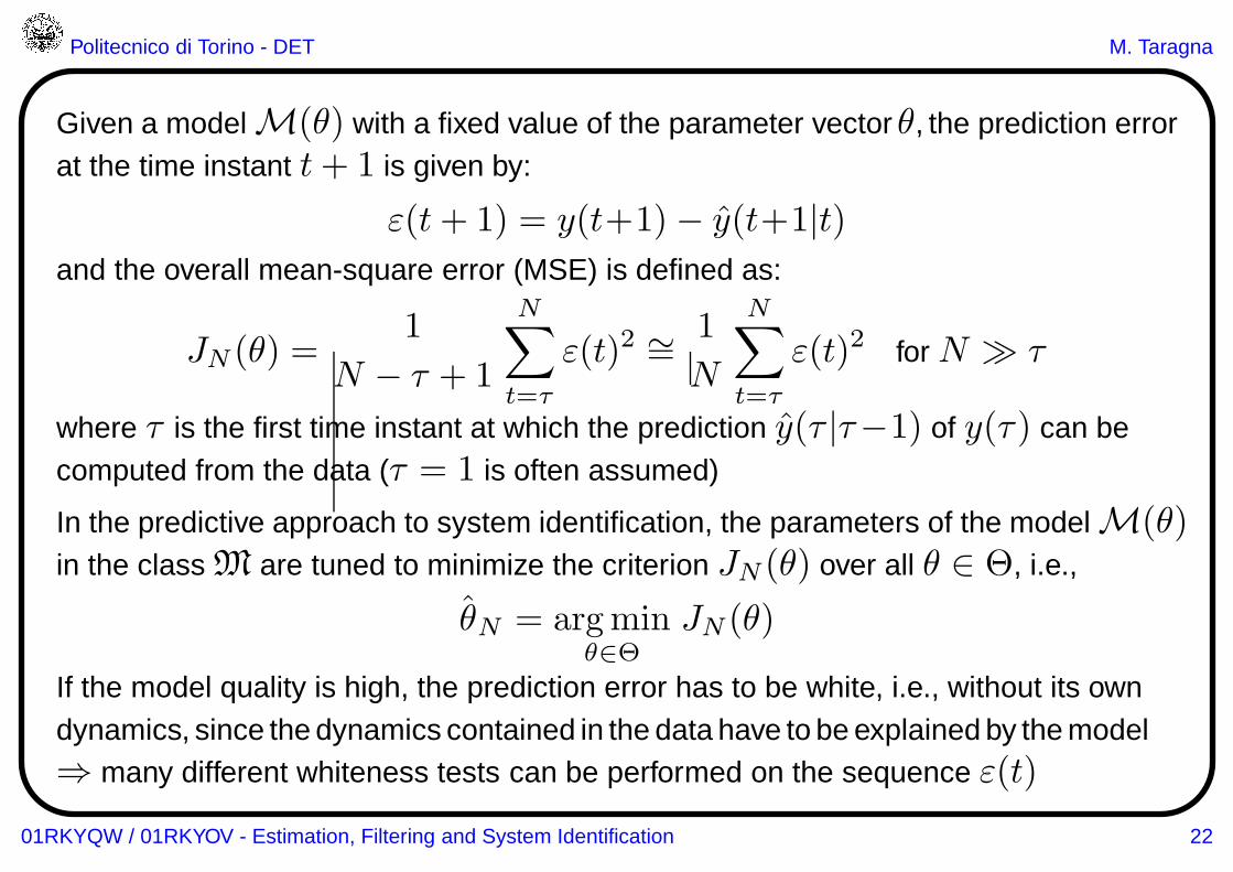
Given a model M(θ) with a fixed value of the parameter vectorθ, the prediction errorat the time instant t+ 1 is given by:
ε(t+ 1) = y(t+1)− y(t+1|t)and the overall mean-square error (MSE) is defined as:
JN (θ) =1
N − τ + 1
N∑
t=τ
ε(t)2 ∼= 1
N
N∑
t=τ
ε(t)2 for N ≫ τ
where τ is the first time instant at which the prediction y(τ |τ−1) of y(τ) can becomputed from the data (τ = 1 is often assumed)
In the predictive approach to system identification, the parameters of the model M(θ)in the class M are tuned to minimize the criterion JN (θ) over all θ ∈ Θ, i.e.,
θN = argminθ∈Θ
JN (θ)
If the model quality is high, the prediction error has to be white, i.e., without its owndynamics, since the dynamics contained in the data have to be explained by the model⇒ many different whiteness tests can be performed on the sequence ε(t)
01RKYQW / 01RKYOV - Estimation, Filtering and System Identification 22
Politecnico di Torino - DET M. Taragna
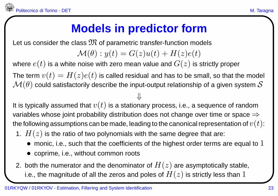
Models in predictor formLet us consider the class M of parametric transfer-function models
M(θ) : y(t) = G(z)u(t) +H(z)e(t)
where e(t) is a white noise with zero mean value and G(z) is strictly proper
The term v(t) = H(z)e(t) is called residual and has to be small, so that the modelM(θ) could satisfactorily describe the input-output relationship of a given system S
⇓It is typically assumed that v(t) is a stationary process, i.e., a sequence of randomvariables whose joint probability distribution does not change over time or space ⇒the following assumptions can be made, leading to the canonical representation ofv(t):1. H(z) is the ratio of two polynomials with the same degree that are:
• monic, i.e., such that the coefficients of the highest order terms are equal to 1• coprime, i.e., without common roots
2. both the numerator and the denominator of H(z) are asymptotically stable,i.e., the magnitude of all the zeros and poles of H(z) is strictly less than 1
01RKYQW / 01RKYOV - Estimation, Filtering and System Identification 23
Politecnico di Torino - DET M. Taragna
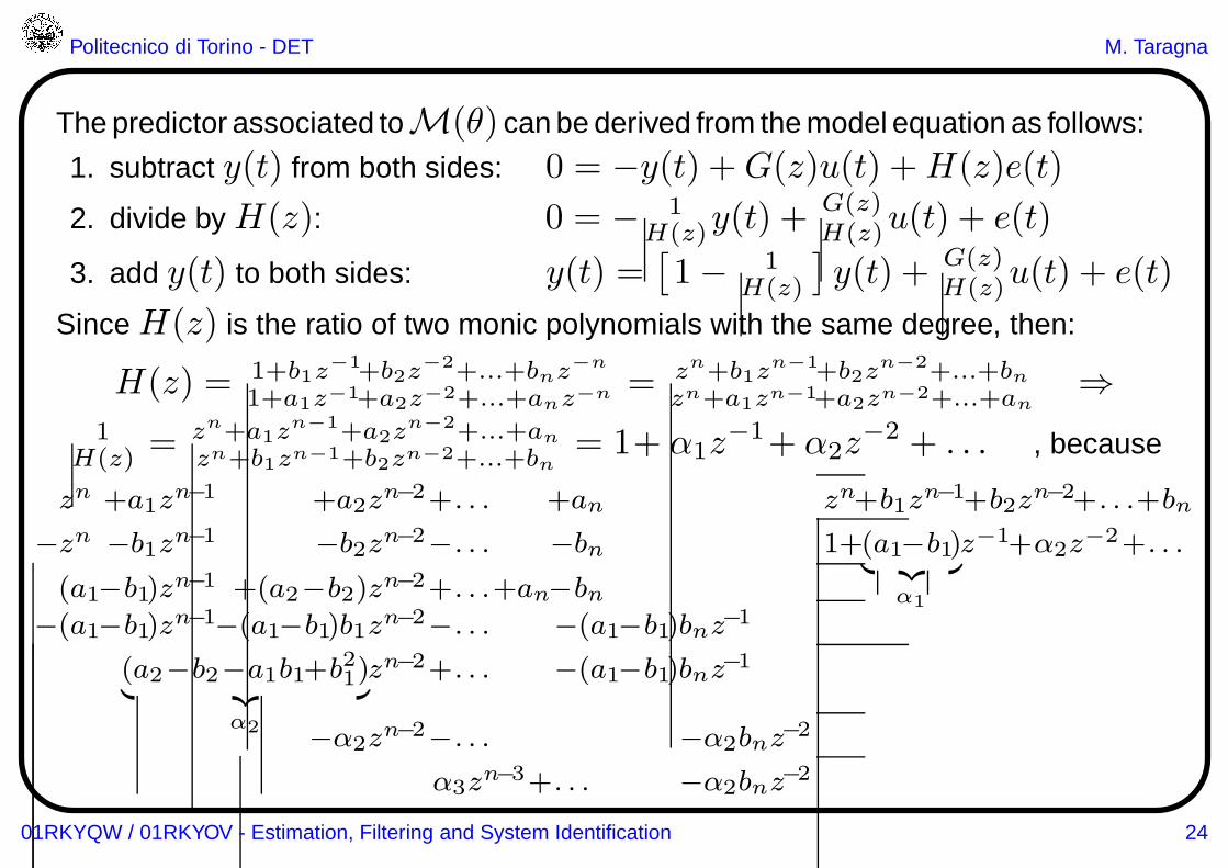
The predictor associated toM(θ) can be derived from the model equation as follows:
1. subtract y(t) from both sides: 0 = −y(t) +G(z)u(t) +H(z)e(t)
2. divide by H(z): 0 = − 1H(z)y(t) +
G(z)H(z)u(t) + e(t)
3. add y(t) to both sides: y(t) =[1− 1
H(z)
]y(t) + G(z)
H(z)u(t) + e(t)
Since H(z) is the ratio of two monic polynomials with the same degree, then:
H(z) = 1+b1z−1+b2z
−2+...+bnz−n
1+a1z−1+a2z−2+...+anz−n = zn+b1zn−1+b2z
n−2+...+bnzn+a1zn−1+a2zn−2+...+an
⇒1
H(z) =zn+a1z
n−1+a2zn−2+...+an
zn+b1zn−1+b2zn−2+...+bn= 1+ α1z
−1+ α2z−2 + . . . , because
zn +a1zn−1 +a2z
n−2+. . . +an zn+b1zn−1+b2z
n−2+. . .+bn
−zn −b1zn−1
−b2zn−2
−. . . −bn 1+(a1−b1)︸ ︷︷ ︸
α1
z−1+α2z−2+. . .
(a1−b1)zn−1 +(a2−b2)zn−2+. . .+an−bn−(a1−b1)zn−1
−(a1−b1)b1zn−2−. . . −(a1−b1)bnz−1
(a2−b2−a1b1+b21)︸ ︷︷ ︸
α2
zn−2+. . . −(a1−b1)bnz−1
−α2zn−2
−. . . −α2bnz−2
α3zn−3+. . . −α2bnz
−2
01RKYQW / 01RKYOV - Estimation, Filtering and System Identification 24
Politecnico di Torino - DET M. Taragna
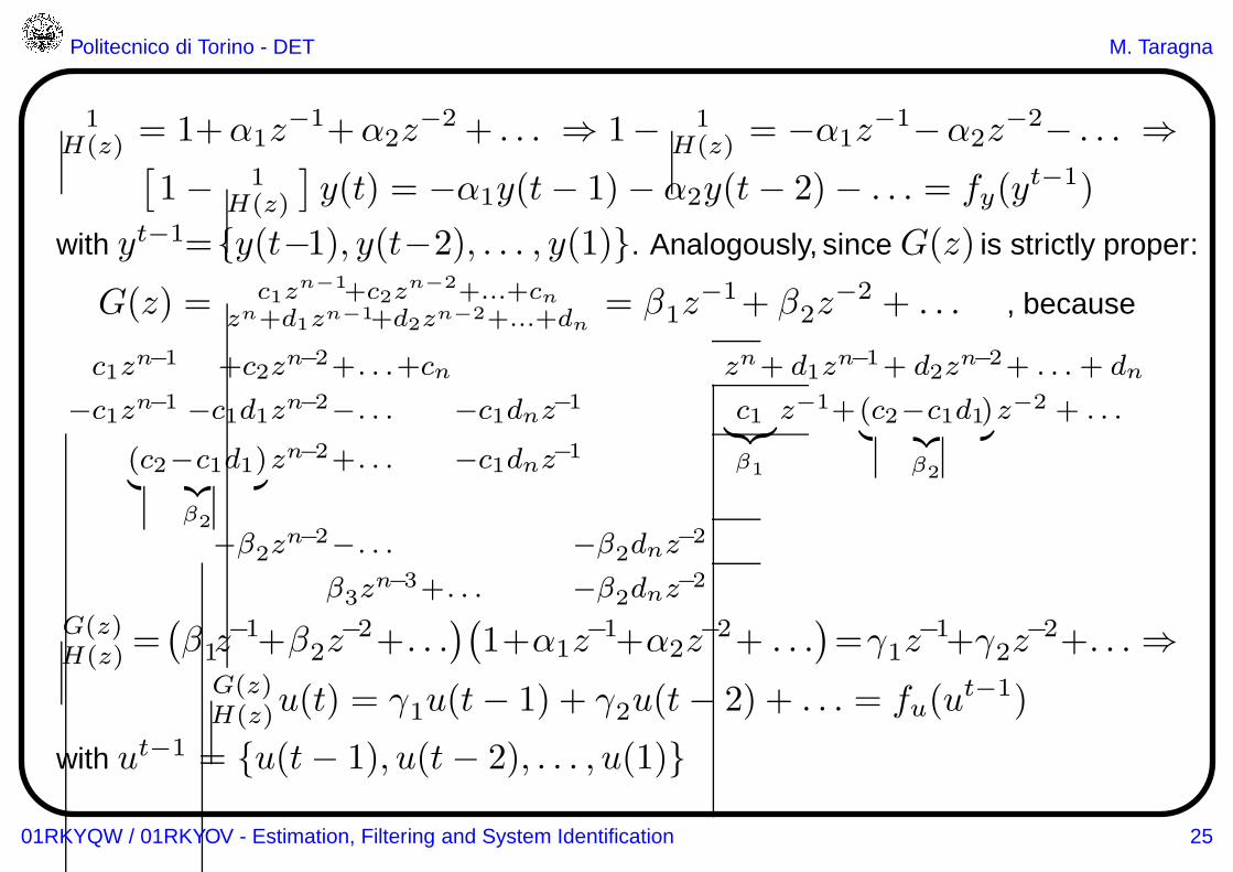
1H(z) = 1+α1z
−1+α2z−2 + . . . ⇒ 1− 1
H(z) = −α1z−1−α2z
−2− . . . ⇒[1− 1
H(z)
]y(t) = −α1y(t− 1)− α2y(t− 2)− . . . = fy(y
t−1)
with yt−1={y(t−1), y(t−2), . . . , y(1)}. Analogously, since G(z) is strictly proper:
G(z) = c1zn−1+c2z
n−2+...+cnzn+d1zn−1+d2zn−2+...+dn
= β1z−1+ β2z
−2 + . . . , because
c1zn−1 +c2z
n−2+. . .+cn zn+ d1zn−1+ d2z
n−2+ . . .+ dn
−c1zn−1
−c1d1zn−2
−. . . −c1dnz−1 c1
︸︷︷︸
β1
z−1+(c2−c1d1)︸ ︷︷ ︸
β2
z−2 + . . .
(c2−c1d1)︸ ︷︷ ︸
β2
zn−2+. . . −c1dnz−1
−β2zn−2
−. . . −β2dnz−2
β3zn−3+. . . −β2dnz
−2
G(z)H(z) =
(β1z
−1+β2z−2+. . .
)(1+α1z
−1+α2z−2+ . . .
)=γ1z
−1+γ2z−2+. . .⇒
G(z)H(z)u(t) = γ1u(t− 1) + γ2u(t− 2) + . . . = fu(u
t−1)
with ut−1 = {u(t− 1), u(t− 2), . . . , u(1)}
01RKYQW / 01RKYOV - Estimation, Filtering and System Identification 25
Politecnico di Torino - DET M. Taragna
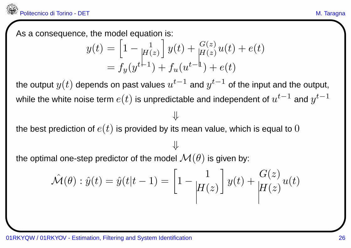
As a consequence, the model equation is:
y(t) =[
1− 1H(z)
]
y(t) + G(z)H(z)u(t) + e(t)
= fy(yt−1) + fu(u
t−1) + e(t)
the output y(t) depends on past values ut−1 and yt−1 of the input and the output,
while the white noise term e(t) is unpredictable and independent of ut−1 and yt−1
⇓the best prediction of e(t) is provided by its mean value, which is equal to 0
⇓the optimal one-step predictor of the model M(θ) is given by:
M(θ) : y(t) = y(t|t− 1) =
[
1− 1
H(z)
]
y(t) +G(z)
H(z)u(t)
01RKYQW / 01RKYOV - Estimation, Filtering and System Identification 26
Politecnico di Torino - DET M. Taragna
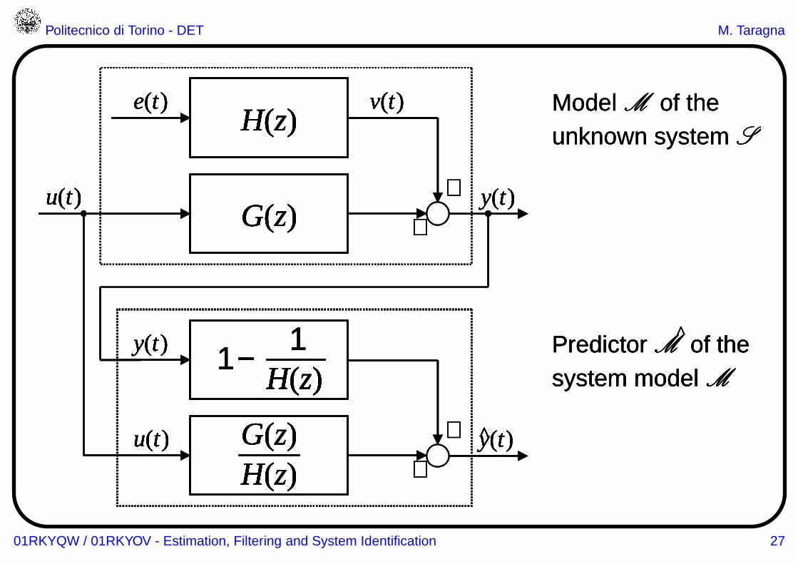
+
+y(t)
e(t) v(t)H(z)
u(t)G(z)
+
+
y(t) 1 −H(z)
1
u(t)
H(z)G(z) y(t)^
Model M of theunknown system S
Predictor M of thesystem model M
^
+
+y(t)
e(t) v(t)H(z)
u(t)G(z)
+
+
y(t) 1 −H(z)
1
u(t)
H(z)G(z) y(t)^
+
+y(t)
e(t) v(t)H(z)
u(t)G(z)
+
+y(t)
e(t) v(t)H(z)
e(t) v(t)H(z)H(z)
u(t)G(z)
u(t)G(z)G(z)
+
+
y(t) 1 −H(z)
1
u(t)
H(z)G(z) y(t)^+
+
y(t) 1 −H(z)
1y(t) 1 −H(z)
11 −H(z)
11 −H(z)
1H(z)
1
u(t)
H(z)G(z)u(t)
H(z)G(z)H(z)G(z) y(t)y(t)^
Model M of theunknown system SModel M of theunknown system S
Predictor M of thesystem model M
^Predictor M of thesystem model MPredictor M of thesystem model M
^
01RKYQW / 01RKYOV - Estimation, Filtering and System Identification 27
Politecnico di Torino - DET M. Taragna
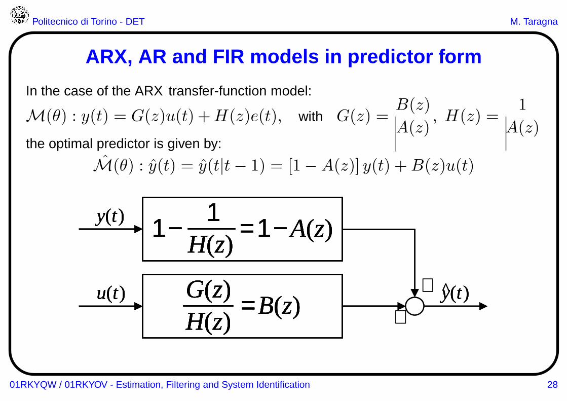
ARX, AR and FIR models in predictor form
In the case of the ARX transfer-function model:
M(θ) : y(t) = G(z)u(t) +H(z)e(t), with G(z) =B(z)
A(z), H(z) =
1
A(z)the optimal predictor is given by:
M(θ) : y(t) = y(t|t− 1) = [1− A(z)] y(t) +B(z)u(t)
+
+
y(t) 1 − = 1 − A(z)H(z)
1
y(t)^u(t)
H(z)G(z) = B(z)
+
+
y(t) 1 − = 1 − A(z)H(z)
1y(t) 1 − = 1 − A(z)H(z)
11 − = 1 − A(z)H(z)
1H(z)
1
y(t)y(t)^u(t)
H(z)G(z) = B(z)
u(t)
H(z)G(z) = B(z)H(z)G(z)H(z)G(z) = B(z)
01RKYQW / 01RKYOV - Estimation, Filtering and System Identification 28
Politecnico di Torino - DET M. Taragna
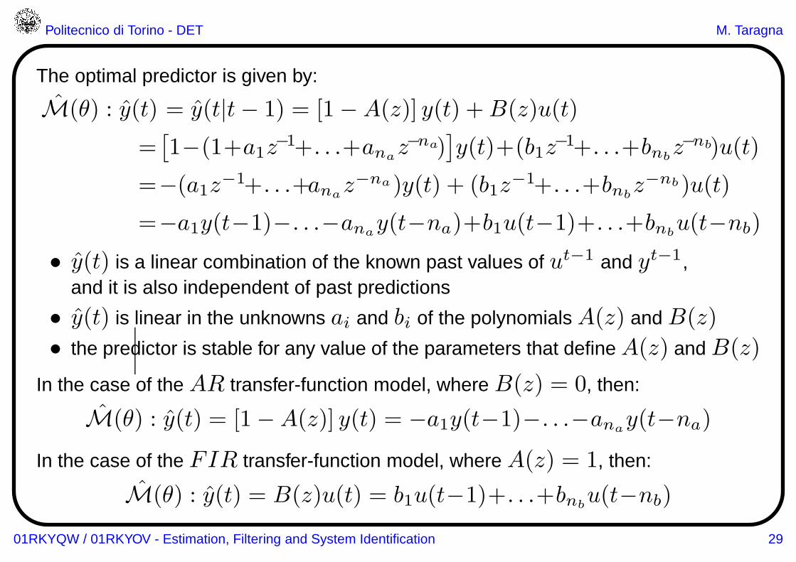
The optimal predictor is given by:
M(θ) : y(t) = y(t|t− 1) = [1− A(z)] y(t) +B(z)u(t)
=[1−(1+a1z
−1+. . .+anaz−na)
]y(t)+(b1z
−1+. . .+bnbz−nb)u(t)
=−(a1z−1+. . .+ana
z−na)y(t) + (b1z−1+. . .+bnb
z−nb)u(t)
=−a1y(t−1)−. . .−anay(t−na)+b1u(t−1)+. . .+bnb
u(t−nb)
• y(t) is a linear combination of the known past values of ut−1 and yt−1,and it is also independent of past predictions
• y(t) is linear in the unknowns ai and bi of the polynomials A(z) and B(z)
• the predictor is stable for any value of the parameters that defineA(z) and B(z)
In the case of the AR transfer-function model, where B(z) = 0, then:
M(θ) : y(t) = [1−A(z)] y(t) = −a1y(t−1)−. . .−anay(t−na)
In the case of the FIR transfer-function model, where A(z) = 1, then:
M(θ) : y(t) = B(z)u(t) = b1u(t−1)+. . .+bnbu(t−nb)
01RKYQW / 01RKYOV - Estimation, Filtering and System Identification 29
Politecnico di Torino - DET M. Taragna
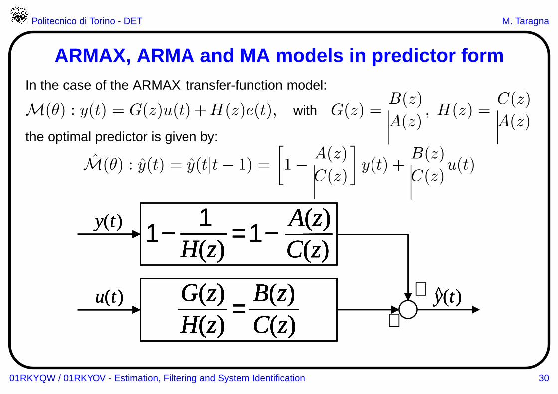
ARMAX, ARMA and MA models in predictor formIn the case of the ARMAX transfer-function model:
M(θ) : y(t) = G(z)u(t) +H(z)e(t), with G(z) =B(z)
A(z), H(z) =
C(z)
A(z)the optimal predictor is given by:
M(θ) : y(t) = y(t|t− 1) =
[
1− A(z)
C(z)
]
y(t) +B(z)
C(z)u(t)
+
+y(t)^u(t)
H(z)G(z) =
C(z)B(z)
y(t) 1 − = 1 −H(z)
1C(z)A(z)
+
+y(t)y(t)^u(t)
H(z)G(z) =
C(z)B(z)u(t)
H(z)G(z) =
C(z)B(z)
H(z)G(z) =
C(z)B(z)
H(z)G(z)H(z)G(z) =
C(z)B(z)C(z)B(z)
y(t) 1 − = 1 −H(z)
1C(z)A(z)y(t) 1 − = 1 −
H(z)1
C(z)A(z)1 − = 1 −
H(z)1
H(z)1
C(z)A(z)C(z)A(z)
01RKYQW / 01RKYOV - Estimation, Filtering and System Identification 30
Politecnico di Torino - DET M. Taragna
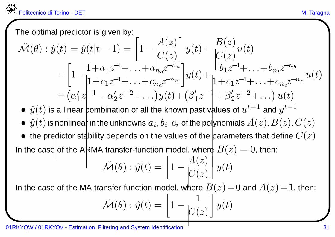
The optimal predictor is given by:
M(θ) : y(t) = y(t|t− 1) =
[
1− A(z)
C(z)
]
y(t) +B(z)
C(z)u(t)
=
[
1− 1+a1z−1+. . .+ana
z−na
1+c1z−1+. . .+cncz−nc
]
y(t)+b1z
−1+. . .+bnbz−nb
1+c1z−1+. . .+cncz−nc
u(t)
=(α′
1z−1+ α′
2z−2+. . .
)y(t)+
(β′
1z−1+ β′
2z−2+. . .
)u(t)
• y(t) is a linear combination of all the known past values of ut−1 and yt−1
• y(t) is nonlinear in the unknowns ai, bi, ci of the polynomials A(z),B(z),C(z)
• the predictor stability depends on the values of the parameters that define C(z)
In the case of the ARMA transfer-function model, where B(z) = 0, then:
M(θ) : y(t) =
[
1− A(z)
C(z)
]
y(t)
In the case of the MA transfer-function model, where B(z)=0 and A(z)=1, then:
M(θ) : y(t) =
[
1− 1
C(z)
]
y(t)
01RKYQW / 01RKYOV - Estimation, Filtering and System Identification 31
Politecnico di Torino - DET M. Taragna
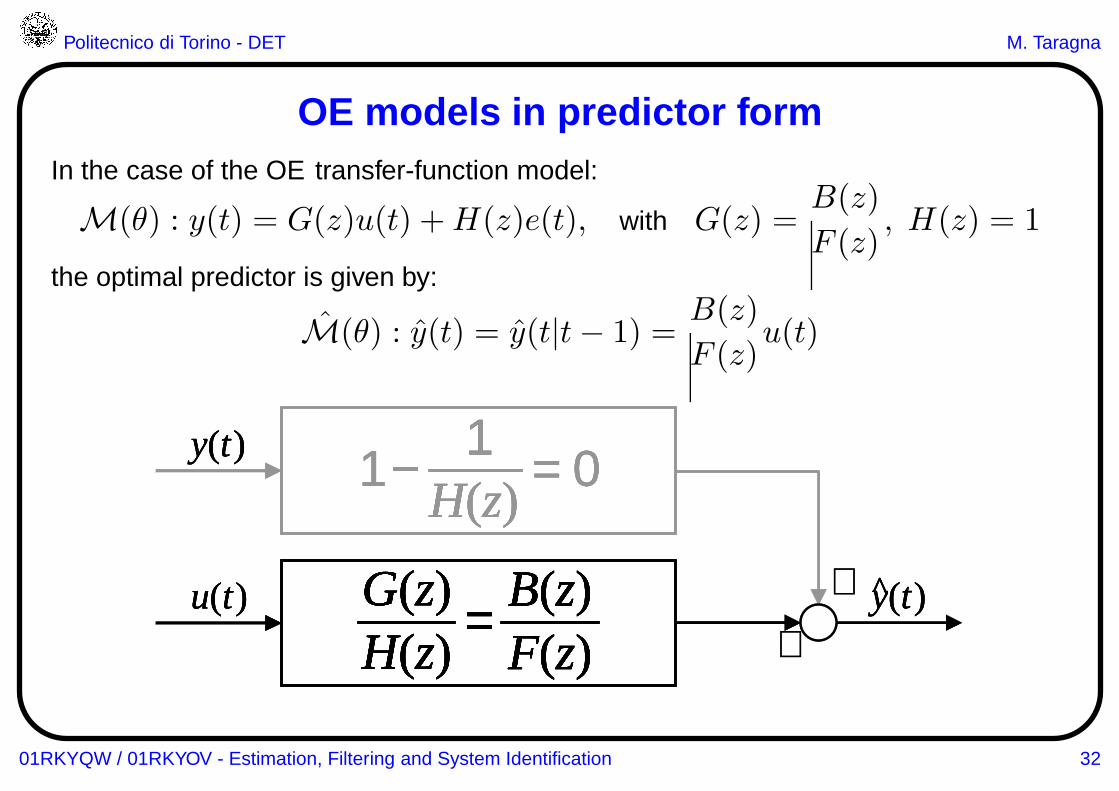
OE models in predictor formIn the case of the OE transfer-function model:
M(θ) : y(t) = G(z)u(t) +H(z)e(t), with G(z) =B(z)
F (z), H(z) = 1
the optimal predictor is given by:
M(θ) : y(t) = y(t|t− 1) =B(z)
F (z)u(t)
+
+y(t)^u(t)
H(z)G(z) =
F(z)B(z)
y(t) 1 − = 0H(z)
1
+
+y(t)y(t)^u(t)
H(z)G(z) =
F(z)B(z)u(t)
H(z)G(z) =
F(z)B(z)
H(z)G(z) =
F(z)B(z)
H(z)G(z)H(z)G(z) =
F(z)B(z)F(z)B(z)
y(t) 1 − = 0H(z)
1y(t) 1 − = 0H(z)
11 − = 0H(z)
1H(z)
1
01RKYQW / 01RKYOV - Estimation, Filtering and System Identification 32
Politecnico di Torino - DET M. Taragna
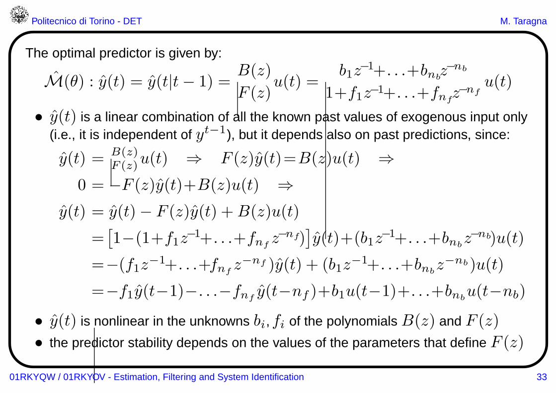
The optimal predictor is given by:
M(θ) : y(t) = y(t|t− 1) =B(z)
F (z)u(t) =
b1z−1+. . .+bnb
z−nb
1+f1z−1+. . .+fnfz−nf
u(t)
• y(t) is a linear combination of all the known past values of exogenous input only(i.e., it is independent of yt−1), but it depends also on past predictions, since:
y(t) = B(z)F (z)u(t) ⇒ F (z)y(t)=B(z)u(t) ⇒
0 = −F (z)y(t)+B(z)u(t) ⇒y(t) = y(t)− F (z)y(t) +B(z)u(t)
=[1−(1+f1z
−1+. . .+fnfz−nf)
]y(t)+(b1z
−1+. . .+bnbz−nb)u(t)
=−(f1z−1+. . .+fnf
z−nf )y(t) + (b1z−1+. . .+bnb
z−nb)u(t)
=−f1y(t−1)−. . .−fnfy(t−nf )+b1u(t−1)+. . .+bnb
u(t−nb)
• y(t) is nonlinear in the unknowns bi,fi of the polynomials B(z) and F (z)
• the predictor stability depends on the values of the parameters that define F (z)
01RKYQW / 01RKYOV - Estimation, Filtering and System Identification 33
Politecnico di Torino - DET M. Taragna
Asymptotic analysis ofprediction-error identification methods
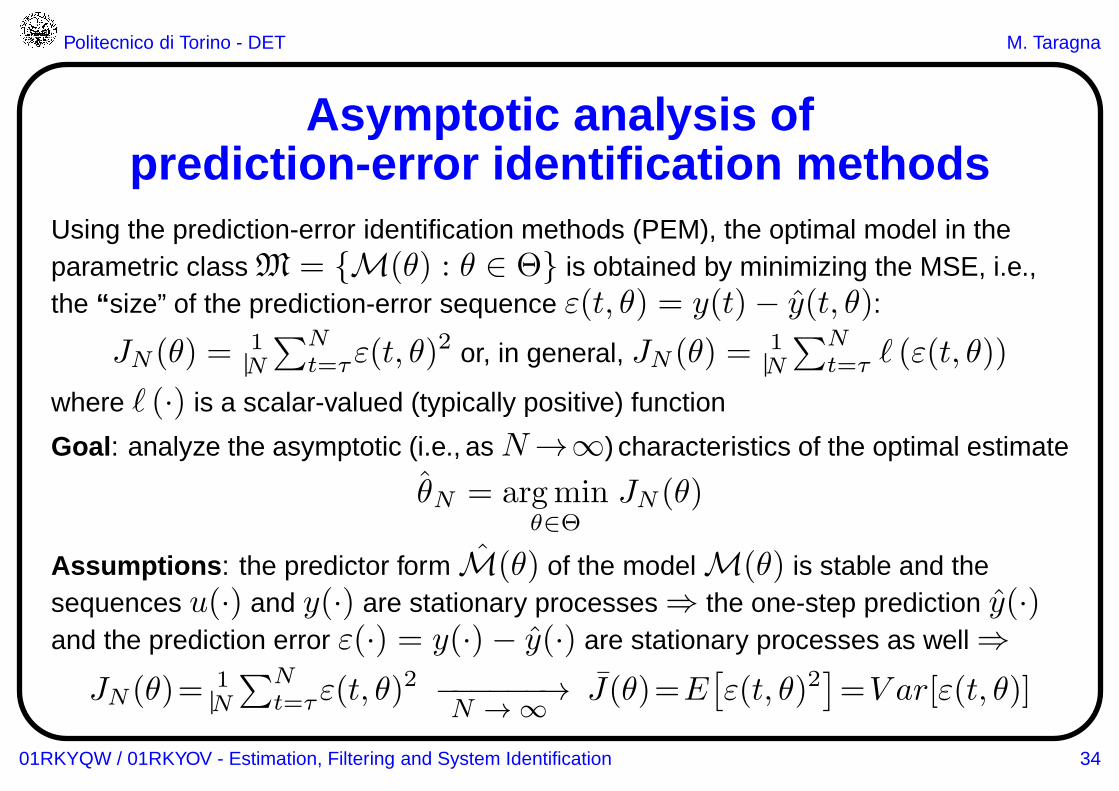
Using the prediction-error identification methods (PEM), the optimal model in theparametric class M = {M(θ) : θ ∈ Θ} is obtained by minimizing the MSE, i.e.,the “ size” of the prediction-error sequence ε(t, θ) = y(t)− y(t, θ):
JN (θ) = 1N
∑Nt=τε(t, θ)
2 or, in general, JN (θ) = 1N
∑Nt=τ ℓ (ε(t, θ))
where ℓ (·) is a scalar-valued (typically positive) function
Goal : analyze the asymptotic (i.e., asN→∞) characteristics of the optimal estimate
θN = argminθ∈Θ
JN (θ)
Assumptions : the predictor form M(θ) of the model M(θ) is stable and thesequences u(·) and y(·) are stationary processes ⇒ the one-step prediction y(·)and the prediction error ε(·) = y(·)− y(·) are stationary processes as well ⇒JN (θ)= 1
N
∑Nt=τε(t, θ)
2 −−−−−−→N → ∞
J(θ)=E[ε(t, θ)2
]=V ar[ε(t, θ)]
01RKYQW / 01RKYOV - Estimation, Filtering and System Identification 34
Politecnico di Torino - DET M. Taragna
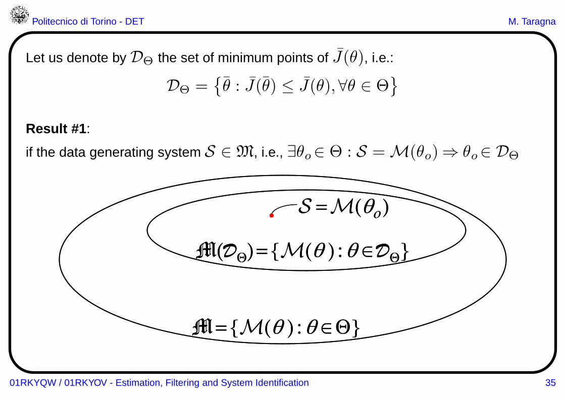
Let us denote by DΘ the set of minimum points of J(θ), i.e.:
DΘ ={θ : J(θ) ≤ J(θ),∀θ ∈ Θ
}
Result #1 :
if the data generating system S ∈ M, i.e., ∃θo∈ Θ : S = M(θo)⇒ θo∈ DΘ
M={M(θ ) :θ ∈Θ}
M(DΘ)={M(θ ) :θ ∈D
Θ}
S =M(θο)
M={M(θ ) :θ ∈Θ}
M(DΘ)={M(θ ) :θ ∈D
Θ}
S =M(θο)
01RKYQW / 01RKYOV - Estimation, Filtering and System Identification 35
Politecnico di Torino - DET M. Taragna
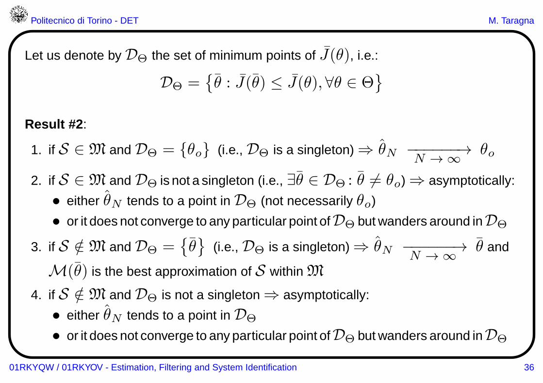
Let us denote by DΘ the set of minimum points of J(θ), i.e.:
DΘ ={θ : J(θ) ≤ J(θ),∀θ ∈ Θ
}
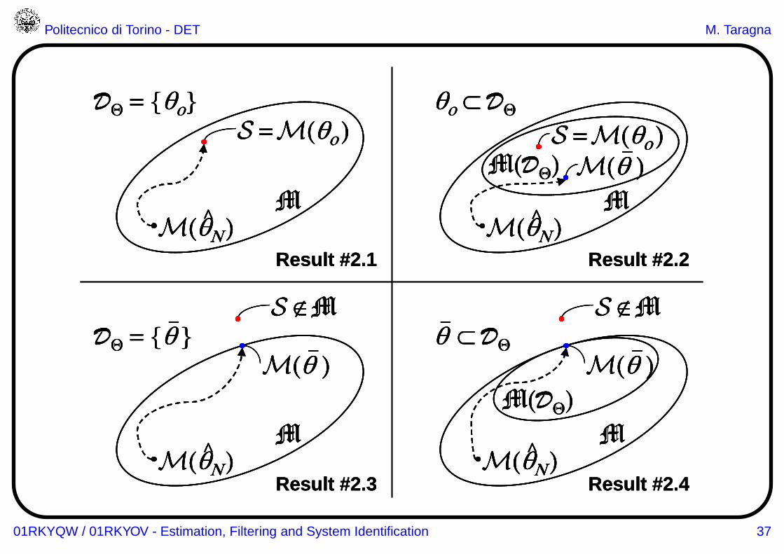
Result #2 :
1. if S ∈ M and DΘ = {θo} (i.e., DΘ is a singleton) ⇒ θN −−−−−−→N → ∞
θo
2. if S ∈ M and DΘ is not a singleton (i.e., ∃θ ∈ DΘ : θ 6= θo) ⇒ asymptotically:
• either θN tends to a point in DΘ (not necessarily θo)
• or it does not converge to any particular point ofDΘ but wanders around inDΘ
3. if S /∈ M and DΘ ={θ}
(i.e., DΘ is a singleton) ⇒ θN −−−−−−→N → ∞
θ and
M(θ) is the best approximation of S within M
4. if S /∈ M and DΘ is not a singleton ⇒ asymptotically:
• either θN tends to a point in DΘ
• or it does not converge to any particular point ofDΘ but wanders around inDΘ
01RKYQW / 01RKYOV - Estimation, Filtering and System Identification 36
Politecnico di Torino - DET M. Taragna
M
S =M(θο)
M(θΝ
)^
DΘ
= {θο}
Result #2.1
MM(θ
Ν)
^
DΘ
= {θ }_ S ∉M
M(θ )_
Result #2.3
MM(θ
Ν)
^
θ ⊂ DΘ
_ S ∉M
M(θ )_
M(DΘ)
Result #2.4
M(DΘ)
MM(θ
Ν)
^
θο
⊂ DΘ
S =M(θο)
M(θ )_
Result #2.2
M
S =M(θο)
M(θΝ
)^
DΘ
= {θο}
Result #2.1
M
S =M(θο)
M(θΝ
)^
DΘ
= {θο}
M
S =M(θο)S =M(θ
ο)
M(θΝ
)^
M(θΝ
)^
DΘ
= {θο}
Result #2.1
MM(θ
Ν)
^
DΘ
= {θ }_ S ∉M
M(θ )_
Result #2.3
MM(θ
Ν)
^
DΘ
= {θ }_ S ∉M
M(θ )_
MM(θ
Ν)
^M(θ
Ν)
^
DΘ
= {θ }_ S ∉MS ∉M
M(θ )_
M(θ )_
Result #2.3
MM(θ
Ν)
^
θ ⊂ DΘ
_ S ∉M
M(θ )_
M(DΘ)
Result #2.4
MM(θ
Ν)
^
θ ⊂ DΘ
_ S ∉M
M(θ )_
M(DΘ)
MM(θ
Ν)
^M(θ
Ν)
^
θ ⊂ DΘ
_ S ∉MS ∉M
M(θ )_
M(θ )_
M(DΘ)
Result #2.4
M(DΘ)
MM(θ
Ν)
^
θο
⊂ DΘ
S =M(θο)
M(θ )_
Result #2.2
M(DΘ)
MM(θ
Ν)
^
θο
⊂ DΘ
S =M(θο)
M(θ )_
M(DΘ)
MM(θ
Ν)
^M(θ
Ν)
^
θο
⊂ DΘ
S =M(θο)S =M(θ
ο)
M(θ )_
M(θ )_
M(θ )_
Result #2.2
01RKYQW / 01RKYOV - Estimation, Filtering and System Identification 37
Politecnico di Torino - DET M. Taragna
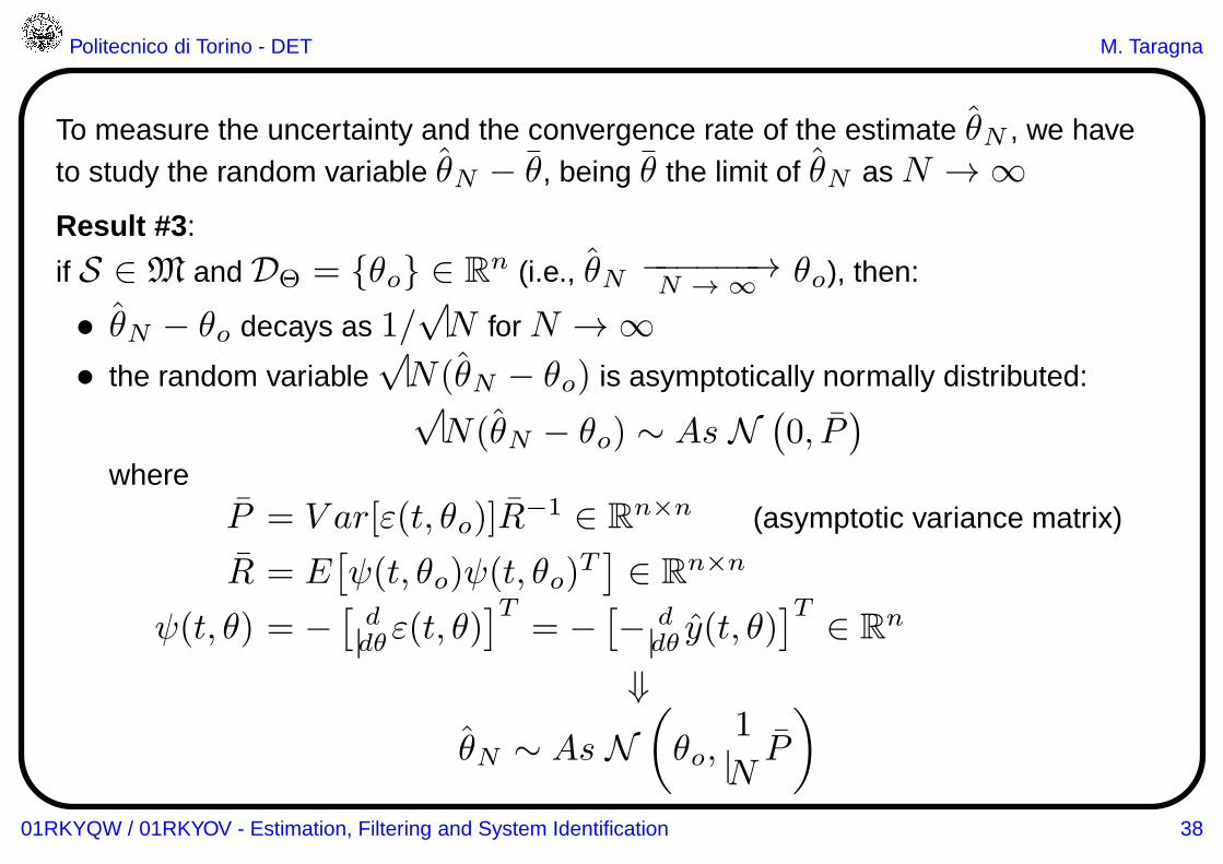
To measure the uncertainty and the convergence rate of the estimate θN , we haveto study the random variable θN − θ, being θ the limit of θN as N → ∞Result #3 :
if S ∈ M and DΘ = {θo} ∈ Rn (i.e., θN −−−−−−→
N → ∞θo), then:
• θN − θo decays as 1/√N for N → ∞
• the random variable√N(θN − θo) is asymptotically normally distributed:√N(θN − θo) ∼ As N
(0, P
)
where
P = V ar[ε(t, θo)]R−1 ∈ R
n×n (asymptotic variance matrix)
R = E[ψ(t, θo)ψ(t, θo)
T]∈ R
n×n
ψ(t, θ) = −[
ddθε(t, θ)
]T= −
[− d
dθ y(t, θ)]T ∈ R
n
⇓θN ∼ As N
(
θo,1
NP
)
01RKYQW / 01RKYOV - Estimation, Filtering and System Identification 38
Politecnico di Torino - DET M. Taragna
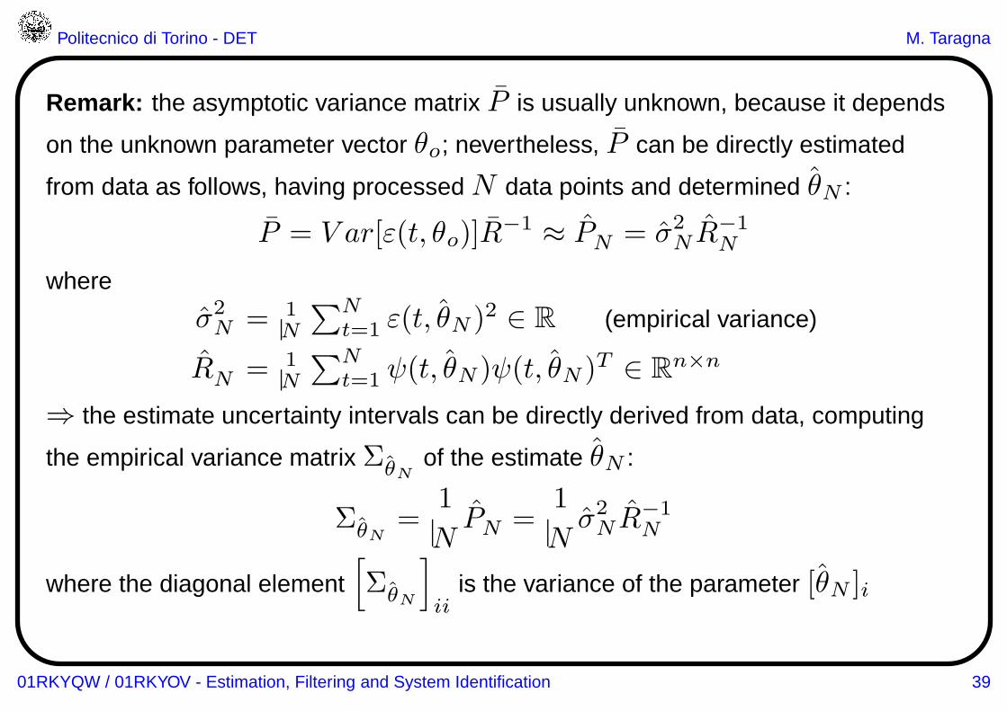
Remark: the asymptotic variance matrix P is usually unknown, because it depends
on the unknown parameter vector θo; nevertheless, P can be directly estimated
from data as follows, having processed N data points and determined θN :
P = V ar[ε(t, θo)]R−1 ≈ PN = σ2
N R−1N
where
σ2N = 1
N
∑Nt=1 ε(t, θN )2 ∈ R (empirical variance)
RN = 1N
∑Nt=1 ψ(t, θN )ψ(t, θN )T ∈ R
n×n
⇒ the estimate uncertainty intervals can be directly derived from data, computing
the empirical variance matrix ΣθNof the estimate θN :
ΣθN=
1
NPN =
1
Nσ2N R
−1N
where the diagonal element[
ΣθN
]
iiis the variance of the parameter [θN ]i
01RKYQW / 01RKYOV - Estimation, Filtering and System Identification 39
Politecnico di Torino - DET M. Taragna
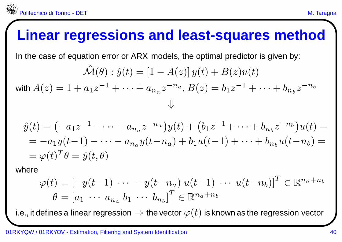
Linear regressions and least-squares methodIn the case of equation error or ARX models, the optimal predictor is given by:
M(θ) : y(t) = [1−A(z)] y(t) +B(z)u(t)
with A(z) = 1 + a1z−1 + · · ·+ ana
z−na , B(z) = b1z−1 + · · ·+ bnb
z−nb
⇓
y(t) =(−a1z−1− · · · − ana
z−na)y(t) +
(b1z
−1+ · · ·+ bnbz−nb
)u(t) =
= −a1y(t−1)− · · · − anay(t−na) + b1u(t−1) + · · ·+ bnb
u(t−nb) =
= ϕ(t)T θ = y(t, θ)
where
ϕ(t) = [−y(t−1) · · · − y(t−na) u(t−1) · · · u(t−nb)]T ∈ R
na+nb
θ = [a1 · · · anab1 · · · bnb
]T ∈ R
na+nb
i.e., it defines a linear regression ⇒ the vector ϕ(t) is known as the regression vector
01RKYQW / 01RKYOV - Estimation, Filtering and System Identification 40
Politecnico di Torino - DET M. Taragna
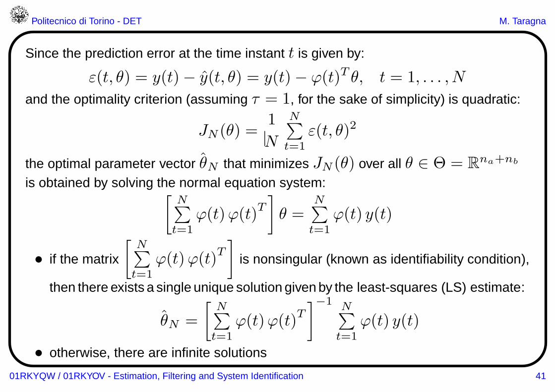
Since the prediction error at the time instant t is given by:
ε(t, θ) = y(t)− y(t, θ) = y(t)− ϕ(t)T θ, t = 1, . . . , N
and the optimality criterion (assuming τ = 1, for the sake of simplicity) is quadratic:
JN (θ) =1
N
N∑
t=1ε(t, θ)2
the optimal parameter vector θN that minimizes JN (θ) over all θ ∈ Θ = Rna+nb
is obtained by solving the normal equation system:[
N∑
t=1ϕ(t)ϕ(t)
T
]
θ =N∑
t=1ϕ(t) y(t)
• if the matrix
[N∑
t=1ϕ(t)ϕ(t)
T
]
is nonsingular (known as identifiability condition),
then there exists a single unique solution given by the least-squares (LS) estimate:
θN =
[N∑
t=1ϕ(t)ϕ(t)
T
]−1 N∑
t=1ϕ(t) y(t)
• otherwise, there are infinite solutions
01RKYQW / 01RKYOV - Estimation, Filtering and System Identification 41
Politecnico di Torino - DET M. Taragna
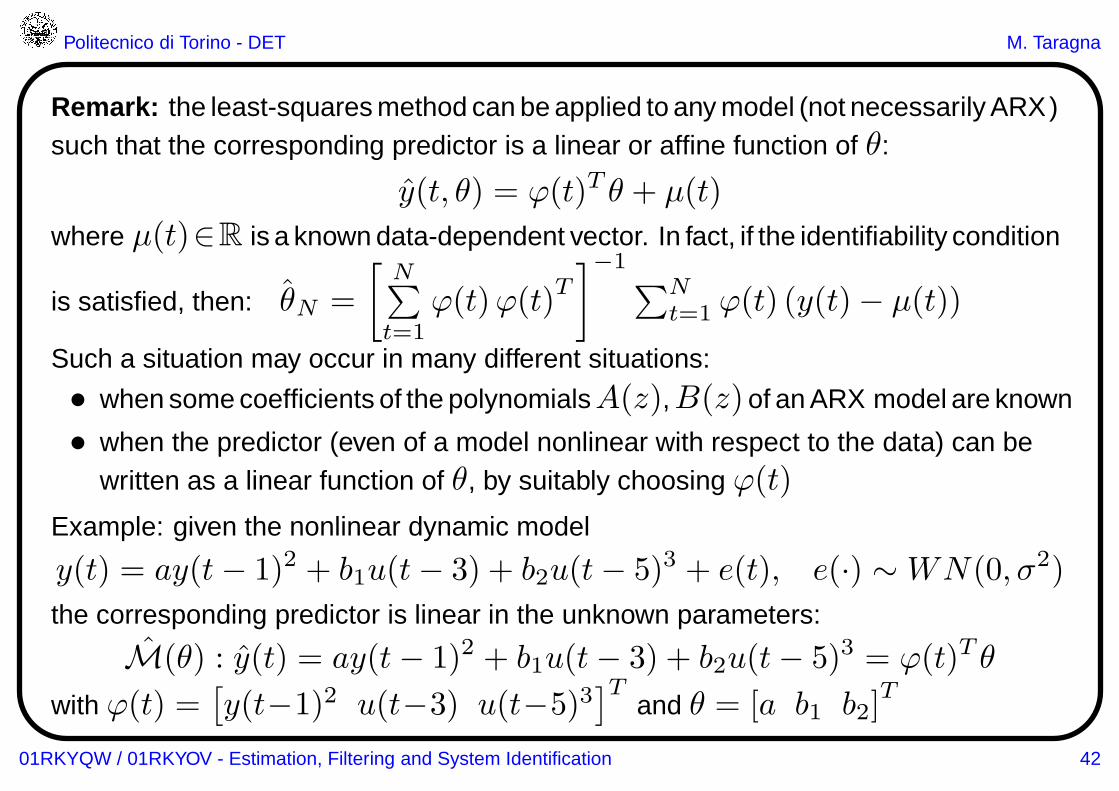
Remark: the least-squares method can be applied to any model (not necessarily ARX )such that the corresponding predictor is a linear or affine function of θ:
y(t, θ) = ϕ(t)T θ + µ(t)
where µ(t)∈R is a known data-dependent vector. In fact, if the identifiability condition
is satisfied, then: θN =
[N∑
t=1ϕ(t)ϕ(t)
T
]−1∑N
t=1 ϕ(t) (y(t)− µ(t))
Such a situation may occur in many different situations:
• when some coefficients of the polynomialsA(z),B(z)of an ARX model are known
• when the predictor (even of a model nonlinear with respect to the data) can bewritten as a linear function of θ, by suitably choosing ϕ(t)
Example: given the nonlinear dynamic model
y(t) = ay(t− 1)2 + b1u(t− 3) + b2u(t− 5)3 + e(t), e(·) ∼WN(0, σ2)
the corresponding predictor is linear in the unknown parameters:
M(θ) : y(t) = ay(t− 1)2 + b1u(t− 3) + b2u(t− 5)3 = ϕ(t)T θ
with ϕ(t) =[y(t−1)2 u(t−3) u(t−5)3
]Tand θ = [a b1 b2]
T
01RKYQW / 01RKYOV - Estimation, Filtering and System Identification 42
Politecnico di Torino - DET M. Taragna
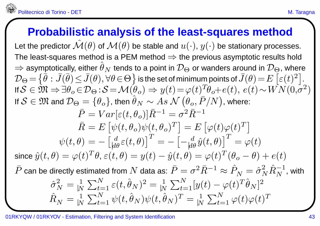
Probabilistic analysis of the least-squares methodLet the predictor M(θ) of M(θ) be stable and u(·), y(·) be stationary processes.The least-squares method is a PEM method ⇒ the previous asymptotic results hold⇒ asymptotically, either θN tends to a point in DΘ or wanders around in DΘ, whereDΘ=
{θ : J(θ)≤ J(θ),∀θ∈Θ
}is the set of minimum points of J(θ)=E
[ε(t)2
].
IfS ∈ M ⇒∃θo∈DΘ :S=M(θo) ⇒ y(t)=ϕ(t)Tθo+e(t), e(t)∼WN(0,σ2)If S ∈ M and DΘ = {θo}, then θN ∼ As N
(θo, P /N
), where:
P = V ar[ε(t, θo)]R−1 = σ2R−1
R = E[ψ(t, θo)ψ(t, θo)
T]= E
[ϕ(t)ϕ(t)T
]
ψ(t, θ) = −[
ddθ ε(t, θ)
]T= −
[− d
dθ y(t, θ)]T
= ϕ(t)
since y(t, θ) = ϕ(t)T θ, ε(t, θ) = y(t)− y(t, θ) = ϕ(t)T (θo − θ) + e(t)
P can be directly estimated from N data as: P = σ2R−1 ≈ PN = σ2N R
−1N , with
σ2N = 1
N
∑Nt=1 ε(t, θN )2 = 1
N
∑Nt=1[y(t)− ϕ(t)T θN ]2
RN = 1N
∑Nt=1 ψ(t, θN )ψ(t, θN )T = 1
N
∑Nt=1 ϕ(t)ϕ(t)
T
01RKYQW / 01RKYOV - Estimation, Filtering and System Identification 43
Politecnico di Torino - DET M. Taragna
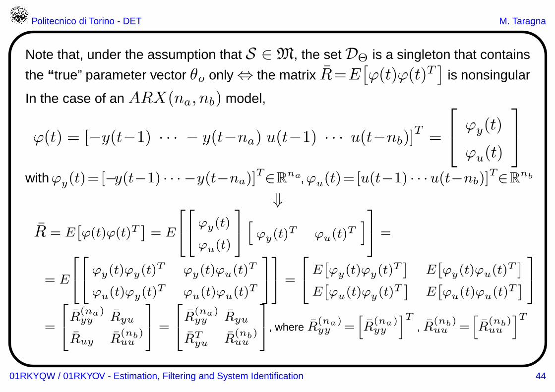
Note that, under the assumption that S ∈ M, the set DΘ is a singleton that contains
the “ true” parameter vector θo only ⇔ the matrix R=E[ϕ(t)ϕ(t)T
]is nonsingular
In the case of an ARX(na, nb) model,
ϕ(t) = [−y(t−1) · · · − y(t−na) u(t−1) · · · u(t−nb)]T=
ϕy(t)
ϕu(t)
withϕy(t)=[−y(t−1) · · · −y(t−na)]T∈R
na,ϕu(t)=[u(t−1) · · ·u(t−nb)]T∈R
nb
⇓
R = E[ϕ(t)ϕ(t)T
]= E
ϕy(t)
ϕu(t)
[
ϕy(t)T ϕu(t)
T]
=
= E
ϕy(t)ϕy(t)
T ϕy(t)ϕu(t)T
ϕu(t)ϕy(t)T ϕu(t)ϕu(t)
T
=
E[ϕy(t)ϕy(t)
T]
E[ϕy(t)ϕu(t)
T]
E[ϕu(t)ϕy(t)
T]
E[ϕu(t)ϕu(t)
T]
=
R
(na)yy Ryu
Ruy R(nb)uu
=
R
(na)yy Ryu
RTyu R
(nb)uu
, where R(na)yy =
[
R(na)yy
]T, R
(nb)uu =
[
R(nb)uu
]T
01RKYQW / 01RKYOV - Estimation, Filtering and System Identification 44
Politecnico di Torino - DET M. Taragna
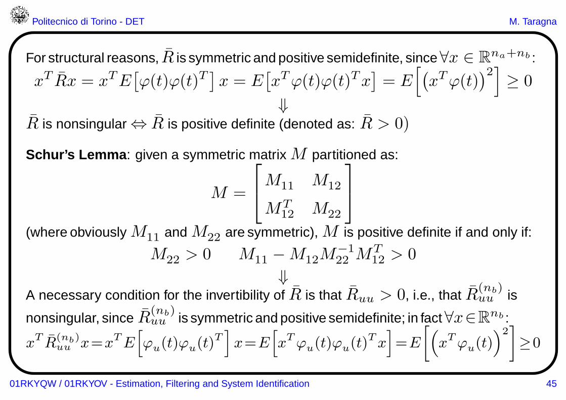
For structural reasons, R is symmetric and positive semidefinite, since∀x ∈ Rna+nb :
xT Rx = xTE[ϕ(t)ϕ(t)T
]x = E
[xTϕ(t)ϕ(t)Tx
]= E
[(xTϕ(t)
)2]
≥ 0
⇓R is nonsingular ⇔ R is positive definite (denoted as: R > 0)
Schur’s Lemma : given a symmetric matrix M partitioned as:
M =
M11 M12
MT12 M22
(where obviouslyM11 and M22 are symmetric), M is positive definite if and only if:
M22 > 0 M11 −M12M−122 M
T12 > 0
⇓A necessary condition for the invertibility of R is that Ruu > 0, i.e., that R
(nb)uu is
nonsingular, since R(nb)uu is symmetric and positive semidefinite; in fact∀x∈R
nb :
xTR
(nb)uu x=x
TE[
ϕu(t)ϕu(t)T]
x=E[
xTϕu(t)ϕu(t)
Tx]
=E
[
(
xTϕu(t)
)2]
≥0
01RKYQW / 01RKYOV - Estimation, Filtering and System Identification 45
Politecnico di Torino - DET M. Taragna
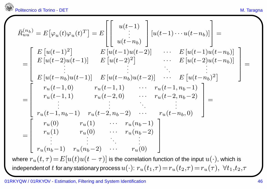
R(nb)uu = E
[ϕu(t)ϕu(t)
T]= E
u(t−1)...
u(t−nb)
[u(t−1) · · ·u(t−nb)]
=
=
E[u(t−1)2
]E [u(t−1)u(t−2)] · · · E [u(t−1)u(t−nb)]
E [u(t−2)u(t−1)] E[u(t−2)2
]· · · E [u(t−2)u(t−nb)]
.
.
....
. . ....
E [u(t−nb)u(t−1)] E [u(t−nb)u(t−2)] · · · E[u(t−nb)
2]
=
=
ru(t−1, 0) ru(t−1, 1) · · · ru(t−1, nb−1)
ru(t−1, 1) ru(t−2, 0) · · · ru(t−2, nb−2)...
.
.
.. . .
.
.
.ru(t−1, nb−1) ru(t−2, nb−2) · · · ru(t−nb, 0)
=
=
ru(0) ru(1) · · · ru(nb−1)
ru(1) ru(0) · · · ru(nb−2)...
.
.
.. . .
.
.
.ru(nb−1) ru(nb−2) · · · ru(0)
where ru(t, τ)=E[u(t)u(t− τ)] is the correlation function of the input u(·), which is
independent of t for any stationary processu(·): ru(t1,τ)=ru(t2,τ)=ru(τ), ∀t1,t2,τ
01RKYQW / 01RKYOV - Estimation, Filtering and System Identification 46
Politecnico di Torino - DET M. Taragna
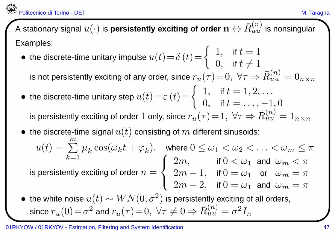
A stationary signal u(·) is persistently exciting of order n⇔ R(n)uu is nonsingular
Examples:
• the discrete-time unitary impulse u(t)=δ (t)=
{
1, if t = 10, if t 6= 1
is not persistently exciting of any order, since ru(τ)=0, ∀τ ⇒ R(n)uu = 0n×n
• the discrete-time unitary step u(t)=ε (t)=
{
1, if t = 1, 2, . . .0, if t = . . . ,−1, 0
is persistently exciting of order 1 only, since ru(τ)=1, ∀τ ⇒ R(n)uu = 1n×n
• the discrete-time signal u(t) consisting of m different sinusoids:
u(t) =m∑
k=1
µk cos(ωkt+ ϕk), where 0 ≤ ω1 < ω2 < . . . < ωm ≤ π
is persistently exciting of order n =
2m, if 0 < ω1 and ωm < π2m− 1, if 0 = ω1 or ωm = π2m− 2, if 0 = ω1 and ωm = π
• the white noise u(t) ∼ WN(0, σ2) is persistently exciting of all orders,
since ru(0)=σ2 and ru(τ)=0, ∀τ 6= 0⇒ R
(n)uu = σ2In
01RKYQW / 01RKYOV - Estimation, Filtering and System Identification 47
Politecnico di Torino - DET M. Taragna
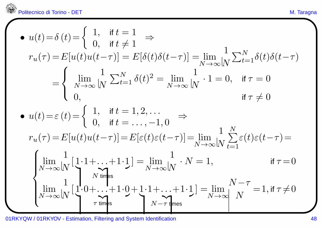
• u(t)=δ (t)={
1, if t = 10, if t 6= 1
⇒
ru(τ)=E[u(t)u(t−τ )] = E[δ(t)δ(t−τ )] = limN→∞
1
N
∑Nt=1δ(t)δ(t−τ)
=
limN→∞
1
N
∑Nt=1 δ(t)
2 = limN→∞
1
N· 1 = 0, if τ = 0
0, if τ 6= 0
• u(t)=ε (t)={
1, if t = 1, 2, . . .0, if t = . . . ,−1, 0
⇒
ru(τ)=E[u(t)u(t−τ )]=E[ε(t)ε(t−τ)]= limN→∞
1
N
N∑
t=1ε(t)ε(t−τ)=
limN→∞
1
N[ 1·1+. . .+1·1︸ ︷︷ ︸
N times
] = limN→∞
1
N·N = 1, if τ=0
limN→∞
1
N[ 1·0+. . .+1·0︸ ︷︷ ︸
τ times
+1·1+. . .+1·1︸ ︷︷ ︸
N−τ times
] = limN→∞
N−τN
=1, if τ 6=0
01RKYQW / 01RKYOV - Estimation, Filtering and System Identification 48
Politecnico di Torino - DET M. Taragna
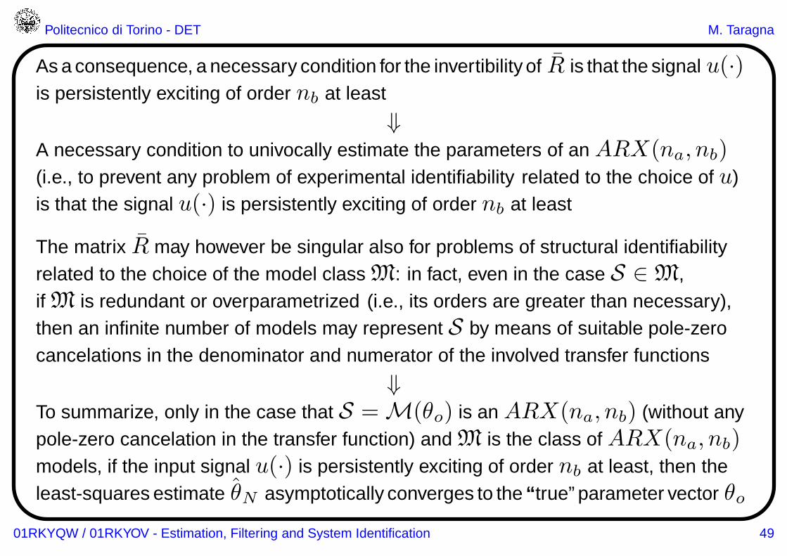
As a consequence, a necessary condition for the invertibility of R is that the signal u(·)is persistently exciting of order nb at least
⇓A necessary condition to univocally estimate the parameters of an ARX(na, nb)(i.e., to prevent any problem of experimental identifiability related to the choice of u)is that the signal u(·) is persistently exciting of order nb at least
The matrix R may however be singular also for problems of structural identifiabilityrelated to the choice of the model class M: in fact, even in the case S ∈ M,if M is redundant or overparametrized (i.e., its orders are greater than necessary),then an infinite number of models may represent S by means of suitable pole-zerocancelations in the denominator and numerator of the involved transfer functions
⇓To summarize, only in the case that S = M(θo) is an ARX(na, nb) (without anypole-zero cancelation in the transfer function) and M is the class of ARX(na, nb)models, if the input signal u(·) is persistently exciting of order nb at least, then theleast-squares estimate θN asymptotically converges to the “ true” parameter vector θo
01RKYQW / 01RKYOV - Estimation, Filtering and System Identification 49
Politecnico di Torino - DET M. Taragna
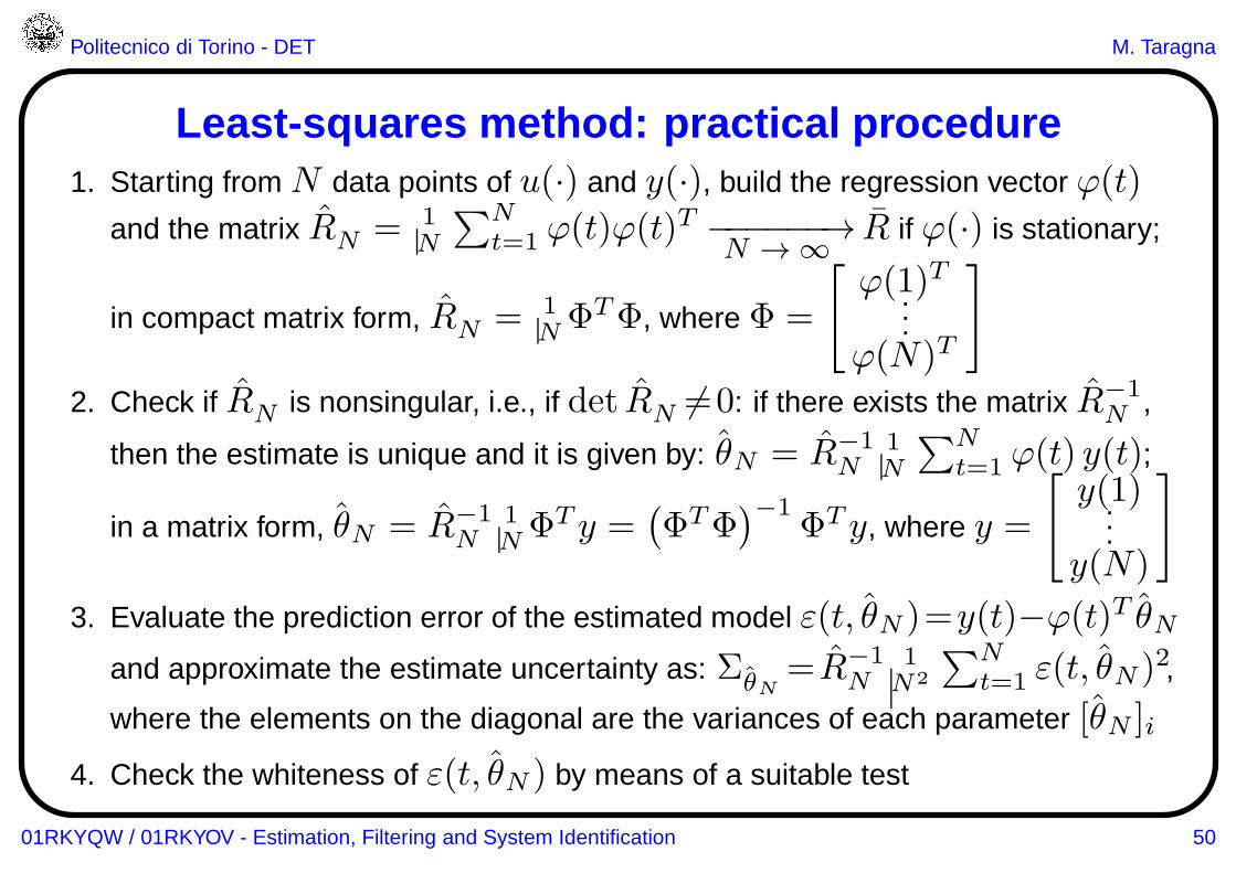
Least-squares method: practical procedure1. Starting from N data points of u(·) and y(·), build the regression vector ϕ(t)
and the matrix RN = 1N
∑Nt=1 ϕ(t)ϕ(t)
T −−−−−−→N → ∞
R if ϕ(·) is stationary;
in compact matrix form, RN = 1NΦTΦ, where Φ =
[ϕ(1)T...ϕ(N)T
]
2. Check if RN is nonsingular, i.e., if det RN 6=0: if there exists the matrix R−1N ,
then the estimate is unique and it is given by: θN = R−1N
1N
∑Nt=1 ϕ(t) y(t);
in a matrix form, θN = R−1N
1NΦT y =
(ΦTΦ
)−1ΦT y, where y =
[y(1)...y(N)
]
3. Evaluate the prediction error of the estimated model ε(t, θN )=y(t)−ϕ(t)T θNand approximate the estimate uncertainty as: ΣθN
=R−1N
1N2
∑Nt=1 ε(t, θN )2,
where the elements on the diagonal are the variances of each parameter [θN ]i
4. Check the whiteness of ε(t, θN ) by means of a suitable test
01RKYQW / 01RKYOV - Estimation, Filtering and System Identification 50

Politecnico di Torino - DET M. Taragna
Anderson’s whiteness testLet ε(·) be the signal under test and N be the (sufficiently large) number of samples
1. Compute the sample correlation function rε(τ)=1
N
N∑
t=τ+1ε(t)ε(t−τ), 0≤τ≤ τ
(τ=25or30), and the normalized sample correlation function ρε(τ)=rε(τ)
rε(0)⇒
if ε(·) is white with zero mean, then ρε(τ) is asymptotically normally distributed:
ρε(τ) ∼ As N(0, 1
N
), ∀τ > 0
moreover, ρε(τ1) and ρε(τ2) are asymptotically uncorrelated ∀τ1 6= τ22. Fix a confidence level α, i.e., the probability α that asymptotically |ρε(τ)| ≤ β,
and evaluate β; in particular, it turns out that: β =
1/√N, for α=68.3%
2/√N, for α=95.4%
3/√N, for α=99.7%
3. The test is failed if the number of τ values such that |ρε(τ)|≤β is less than ⌊ατ⌋,
where ⌊x⌋ denotes the biggest integer less than or equal tox, otherwise it is passed
01RKYQW / 01RKYOV - Estimation, Filtering and System Identification 51
Politecnico di Torino - DET M. Taragna
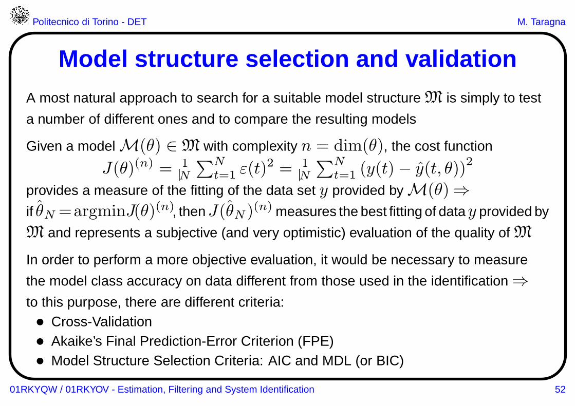
Model structure selection and validationA most natural approach to search for a suitable model structure M is simply to test
a number of different ones and to compare the resulting models
Given a model M(θ) ∈ M with complexity n = dim(θ), the cost function
J(θ)(n) = 1N
∑Nt=1 ε(t)
2 = 1N
∑Nt=1 (y(t)− y(t, θ))2
provides a measure of the fitting of the data set y provided by M(θ)⇒if θN =argminJ(θ)(n), thenJ(θN )(n) measures the best fitting of datay provided by
M and represents a subjective (and very optimistic) evaluation of the quality of M
In order to perform a more objective evaluation, it would be necessary to measure
the model class accuracy on data different from those used in the identification ⇒to this purpose, there are different criteria:• Cross-Validation• Akaike’s Final Prediction-Error Criterion (FPE)• Model Structure Selection Criteria: AIC and MDL (or BIC)
01RKYQW / 01RKYOV - Estimation, Filtering and System Identification 52
Politecnico di Torino - DET M. Taragna
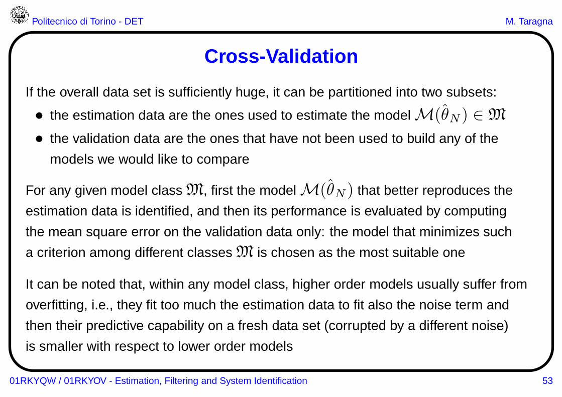
Cross-Validation
If the overall data set is sufficiently huge, it can be partitioned into two subsets:
• the estimation data are the ones used to estimate the model M(θN ) ∈ M
• the validation data are the ones that have not been used to build any of the
models we would like to compare
For any given model class M, first the model M(θN ) that better reproduces the
estimation data is identified, and then its performance is evaluated by computing
the mean square error on the validation data only: the model that minimizes such
a criterion among different classes M is chosen as the most suitable one
It can be noted that, within any model class, higher order models usually suffer from
overfitting, i.e., they fit too much the estimation data to fit also the noise term and
then their predictive capability on a fresh data set (corrupted by a different noise)
is smaller with respect to lower order models
01RKYQW / 01RKYOV - Estimation, Filtering and System Identification 53
Politecnico di Torino - DET M. Taragna
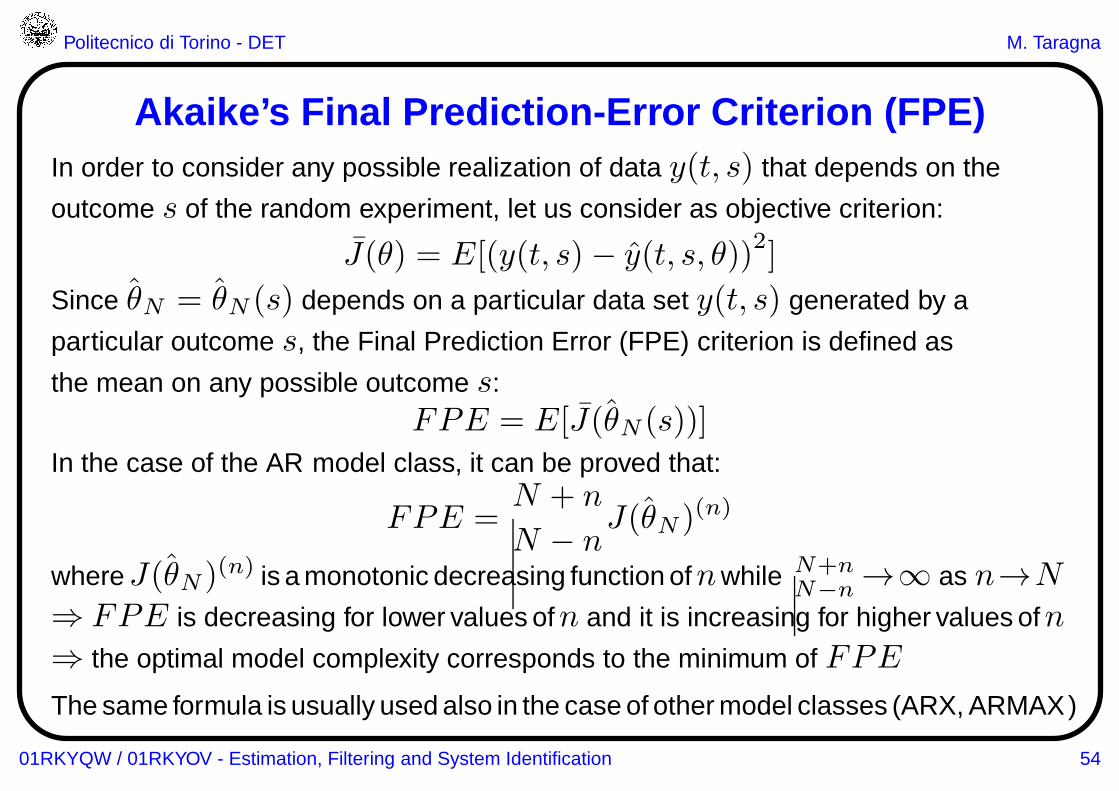
Akaike’s Final Prediction-Error Criterion (FPE)In order to consider any possible realization of data y(t, s) that depends on the
outcome s of the random experiment, let us consider as objective criterion:
J(θ) = E[(y(t, s)− y(t, s, θ))2]
Since θN = θN (s) depends on a particular data set y(t, s) generated by a
particular outcome s, the Final Prediction Error (FPE) criterion is defined as
the mean on any possible outcome s:FPE = E[J(θN (s))]
In the case of the AR model class, it can be proved that:
FPE =N + n
N − nJ(θN )(n)
whereJ(θN )(n) is a monotonic decreasing function ofnwhile N+nN−n →∞ as n→N
⇒ FPE is decreasing for lower values ofn and it is increasing for higher values ofn
⇒ the optimal model complexity corresponds to the minimum of FPE
The same formula is usually used also in the case of other model classes (ARX, ARMAX )
01RKYQW / 01RKYOV - Estimation, Filtering and System Identification 54
Politecnico di Torino - DET M. Taragna
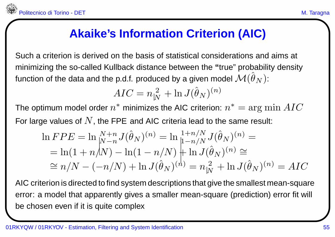
Akaike’s Information Criterion (AIC)
Such a criterion is derived on the basis of statistical considerations and aims atminimizing the so-called Kullback distance between the “ true” probability densityfunction of the data and the p.d.f. produced by a given model M(θN ):
AIC = n 2N + ln J(θN )(n)
The optimum model order n∗ minimizes the AIC criterion: n∗ = arg min AIC
For large values of N , the FPE and AIC criteria lead to the same result:
lnFPE = ln N+nN−nJ(θN )(n) = ln 1+n/N
1−n/N J(θN )(n) =
= ln(1 + n/N)− ln(1− n/N) + ln J(θN )(n) ∼=∼= n/N − (−n/N) + ln J(θN )(n) = n 2
N + ln J(θN )(n) = AIC
AIC criterion is directed to find system descriptions that give the smallest mean-squareerror: a model that apparently gives a smaller mean-square (prediction) error fit willbe chosen even if it is quite complex
01RKYQW / 01RKYOV - Estimation, Filtering and System Identification 55
Politecnico di Torino - DET M. Taragna
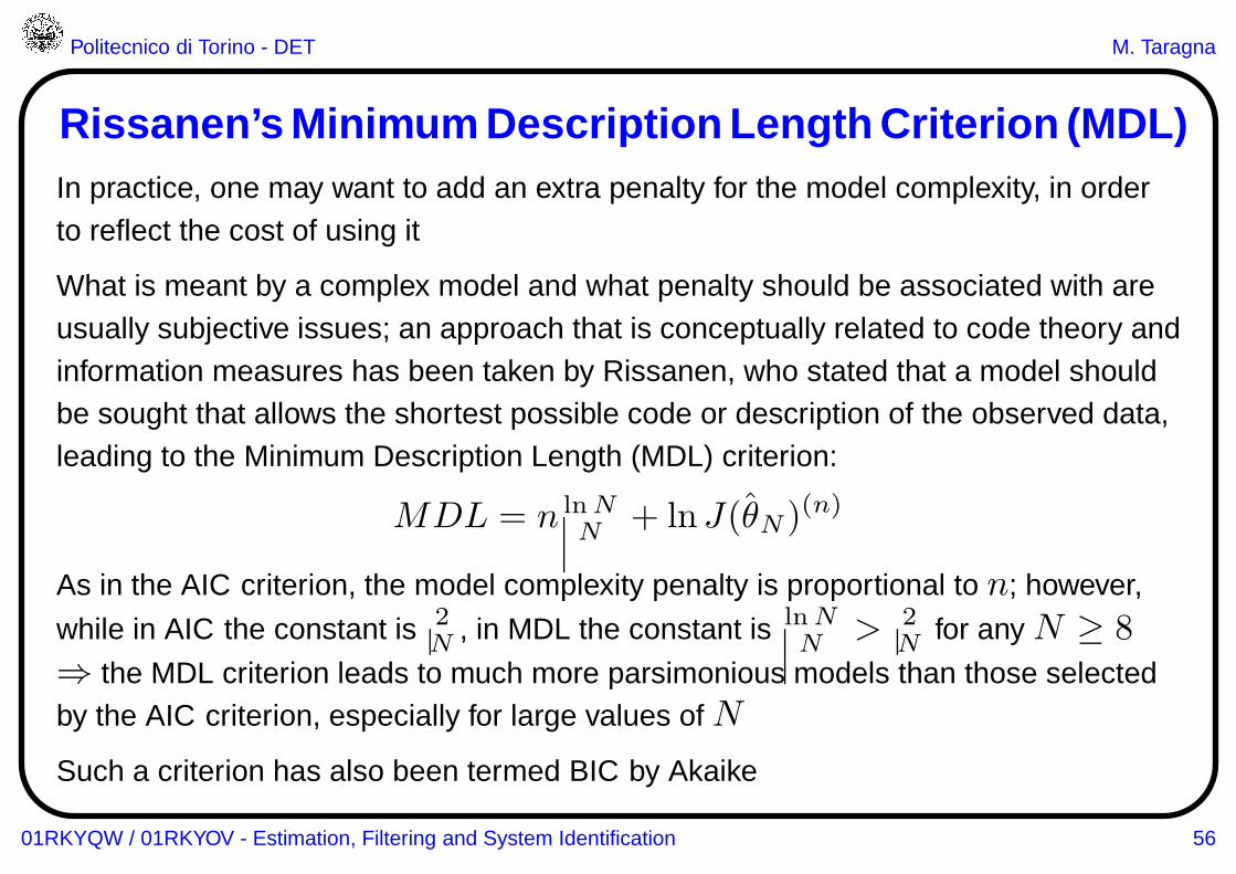
Rissanen’s Minimum Description Length Criterion (MDL)In practice, one may want to add an extra penalty for the model complexity, in orderto reflect the cost of using it
What is meant by a complex model and what penalty should be associated with areusually subjective issues; an approach that is conceptually related to code theory andinformation measures has been taken by Rissanen, who stated that a model shouldbe sought that allows the shortest possible code or description of the observed data,leading to the Minimum Description Length (MDL) criterion:
MDL = n lnNN + ln J(θN )(n)
As in the AIC criterion, the model complexity penalty is proportional to n; however,
while in AIC the constant is 2N , in MDL the constant is lnN
N > 2N for any N ≥ 8
⇒ the MDL criterion leads to much more parsimonious models than those selectedby the AIC criterion, especially for large values of N
Such a criterion has also been termed BIC by Akaike
01RKYQW / 01RKYOV - Estimation, Filtering and System Identification 56
Politecnico di Torino - DET M. Taragna
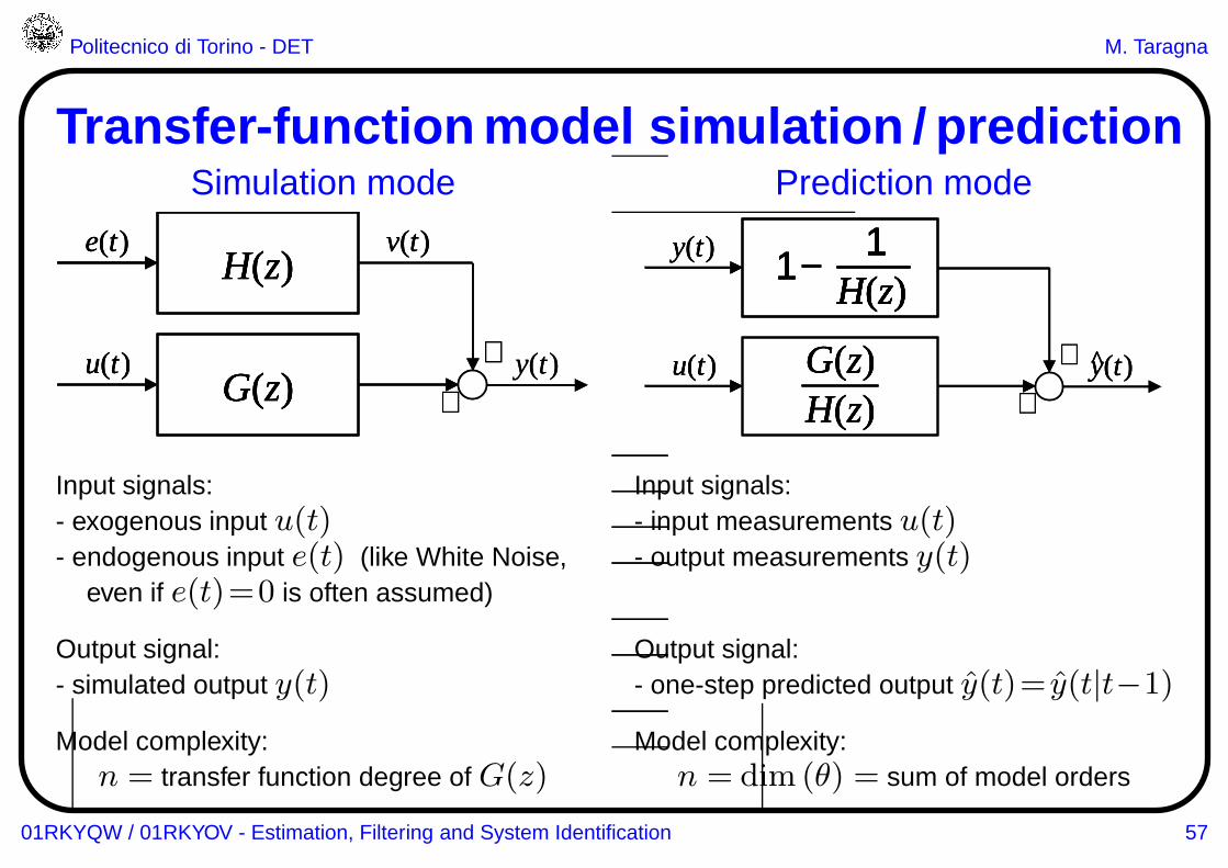
Transfer-function model simulation / predictionSimulation mode Prediction mode
+
+y(t)
e(t) v(t)H(z)
u(t)G(z)
+
+y(t)
e(t) v(t)H(z)
e(t) v(t)H(z)H(z)
u(t)G(z)
u(t)G(z)G(z)
+
+
y(t) 1 −H(z)
1
u(t)
H(z)G(z) y(t)^+
+
y(t) 1 −H(z)
1y(t) 1 −H(z)
11 −H(z)
11 −H(z)
1H(z)
1
u(t)
H(z)G(z)u(t)
H(z)G(z)H(z)G(z) y(t)y(t)^
Input signals: Input signals:- exogenous input u(t) - input measurements u(t)- endogenous input e(t) (like White Noise, - output measurements y(t)
even if e(t)=0 is often assumed)
Output signal: Output signal:- simulated output y(t) - one-step predicted output y(t)= y(t|t−1)
Model complexity: Model complexity:n = transfer function degree of G(z) n = dim (θ) = sum of model orders
01RKYQW / 01RKYOV - Estimation, Filtering and System Identification 57
Politecnico di Torino - DET M. Taragna
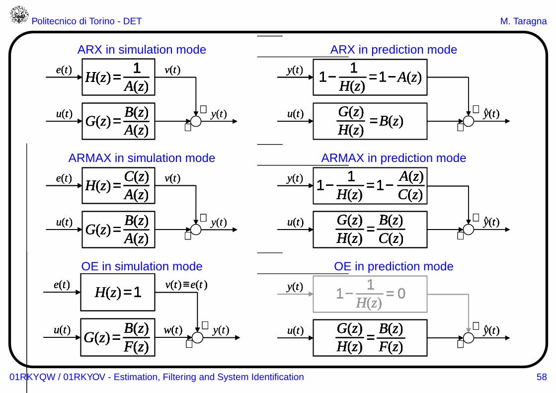
ARX in simulation mode ARX in prediction mode
+
+y(t)
e(t) v(t)H(z)=
A(z)1
u(t)G(z)=
A(z)B(z) +
+y(t)
e(t) v(t)H(z)=
A(z)1e(t) v(t)
H(z)=A(z)
1H(z)=
A(z)1
H(z)=A(z)
1A(z)
1
u(t)G(z)=
A(z)B(z)u(t)
G(z)=A(z)B(z)
G(z)=A(z)B(z)
G(z)=A(z)B(z)A(z)B(z) +
+
y(t) 1 − = 1 − A(z)H(z)
1
y(t)^u(t)
H(z)G(z) = B(z)
+
+
y(t) 1 − = 1 − A(z)H(z)
1y(t) 1 − = 1 − A(z)H(z)
11 − = 1 − A(z)H(z)
1H(z)
1
y(t)y(t)^u(t)
H(z)G(z) = B(z)
u(t)
H(z)G(z) = B(z)H(z)G(z)H(z)G(z) = B(z)
ARMAX in simulation mode ARMAX in prediction mode
+
+y(t)
e(t) v(t)H(z)=
A(z)C(z)
u(t)G(z)=
A(z)B(z) +
+y(t)
e(t) v(t)H(z)=
A(z)C(z)e(t) v(t)
H(z)=A(z)C(z)
H(z)=A(z)C(z)
H(z)=A(z)C(z)A(z)C(z)
u(t)G(z)=
A(z)B(z)u(t)
G(z)=A(z)B(z)
G(z)=A(z)B(z)
G(z)=A(z)B(z)A(z)B(z) +
+y(t)^u(t)
H(z)G(z) =
C(z)B(z)
y(t) 1 − = 1 −H(z)
1C(z)A(z)
+
+y(t)y(t)^u(t)
H(z)G(z) =
C(z)B(z)u(t)
H(z)G(z) =
C(z)B(z)
H(z)G(z) =
C(z)B(z)
H(z)G(z)H(z)G(z) =
C(z)B(z)C(z)B(z)
y(t) 1 − = 1 −H(z)
1C(z)A(z)y(t) 1 − = 1 −
H(z)1
C(z)A(z)1 − = 1 −
H(z)1
H(z)1
C(z)A(z)C(z)A(z)
OE in simulation mode OE in prediction mode
+
+y(t)
e(t) v(t)≡ e(t )H(z)= 1
u(t)G(z)=
F(z)B(z) w(t) +
+y(t)
e(t) v(t)≡ e(t )H(z)= 1e(t) v(t)≡ e(t )H(z)= 1H(z)= 1
u(t)G(z)=
F(z)B(z) w(t)u(t)
G(z)=F(z)B(z)
G(z)=F(z)B(z)
G(z)=F(z)B(z)F(z)B(z) w(t) +
+y(t)^u(t)
H(z)G(z) =
F(z)B(z)
y(t) 1 − = 0H(z)
1
+
+y(t)y(t)^u(t)
H(z)G(z) =
F(z)B(z)u(t)
H(z)G(z) =
F(z)B(z)
H(z)G(z) =
F(z)B(z)
H(z)G(z)H(z)G(z) =
F(z)B(z)F(z)B(z)
y(t) 1 − = 0H(z)
1y(t) 1 − = 0H(z)
11 − = 0H(z)
1H(z)
1
01RKYQW / 01RKYOV - Estimation, Filtering and System Identification 58
Politecnico di Torino - DET M. Taragna
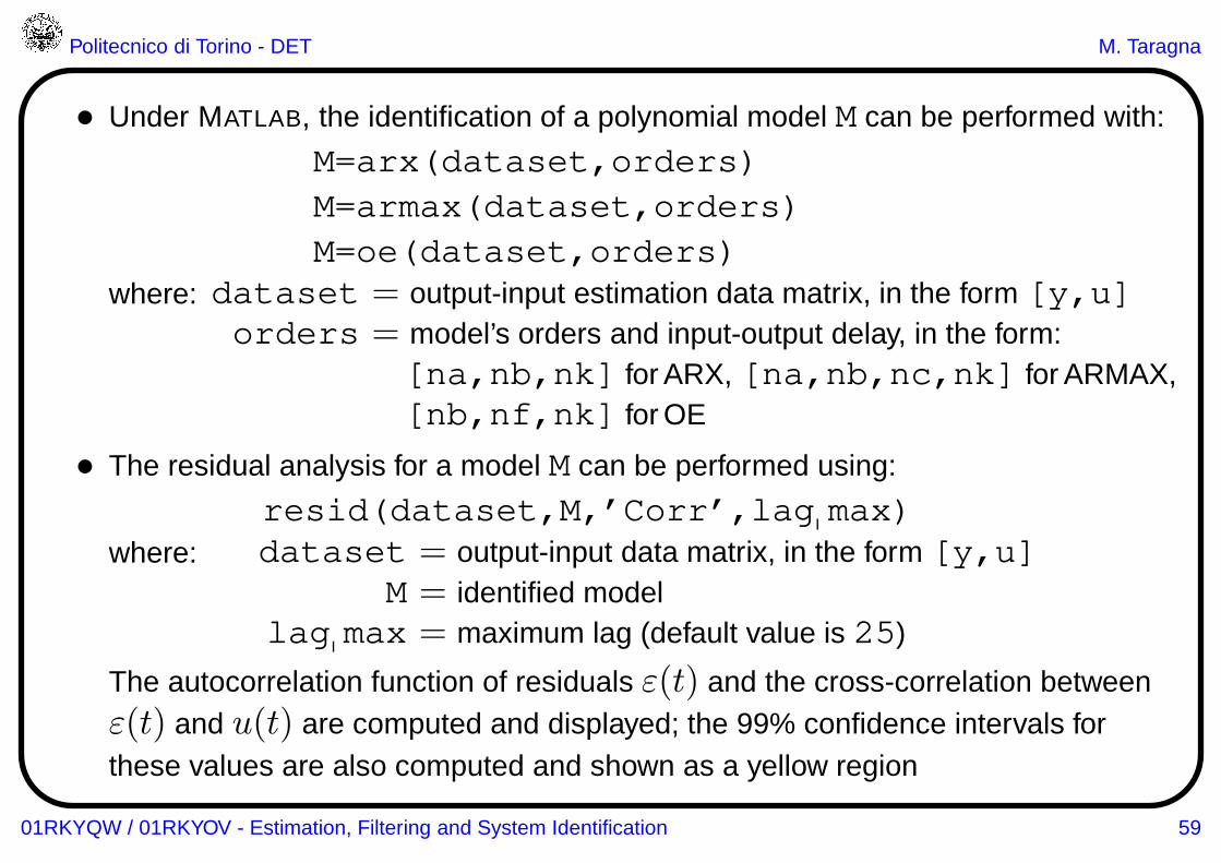
• Under MATLAB, the identification of a polynomial model M can be performed with:
M=arx(dataset,orders)
M=armax(dataset,orders)
M=oe(dataset,orders)
where: dataset = output-input estimation data matrix, in the form [y,u]
orders = model’s orders and input-output delay, in the form:[na,nb,nk] for ARX, [na,nb,nc,nk] for ARMAX,[nb,nf,nk] for OE
• The residual analysis for a model M can be performed using:
resid(dataset,M,’Corr’,lag max)
where: dataset = output-input data matrix, in the form [y,u]
M = identified modellag max = maximum lag (default value is 25)
The autocorrelation function of residuals ε(t) and the cross-correlation betweenε(t) and u(t) are computed and displayed; the 99% confidence intervals forthese values are also computed and shown as a yellow region
01RKYQW / 01RKYOV - Estimation, Filtering and System Identification 59
Politecnico di Torino - DET M. Taragna
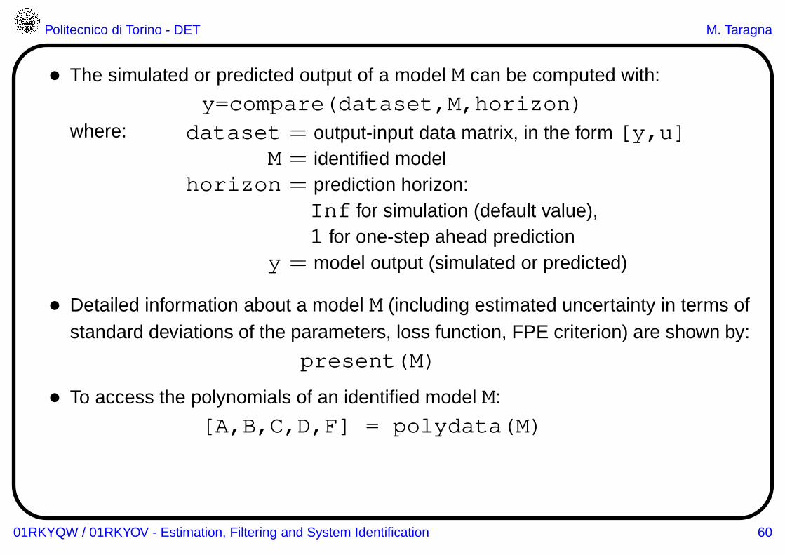
• The simulated or predicted output of a model M can be computed with:
y=compare(dataset,M,horizon)
where: dataset = output-input data matrix, in the form [y,u]
M = identified modelhorizon = prediction horizon:
Inf for simulation (default value),1 for one-step ahead prediction
y = model output (simulated or predicted)
• Detailed information about a model M (including estimated uncertainty in terms ofstandard deviations of the parameters, loss function, FPE criterion) are shown by:
present(M)
• To access the polynomials of an identified model M:
[A,B,C,D,F] = polydata(M)
01RKYQW / 01RKYOV - Estimation, Filtering and System Identification 60
Politecnico di Torino - DET M. Taragna
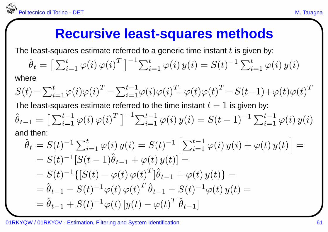
Recursive least-squares methodsThe least-squares estimate referred to a generic time instant t is given by:
θt =[∑t
i=1 ϕ(i)ϕ(i)T ]−1∑t
i=1 ϕ(i) y(i) = S(t)−1 ∑ti=1 ϕ(i) y(i)
where
S(t)=∑t
i=1ϕ(i)ϕ(i)T=∑t−1
i=1ϕ(i)ϕ(i)T+ϕ(t)ϕ(t)
T=S(t−1)+ϕ(t)ϕ(t)
T
The least-squares estimate referred to the time instant t− 1 is given by:
θt−1 =[∑t−1
i=1 ϕ(i)ϕ(i)T ]−1∑t−1
i=1 ϕ(i) y(i) = S(t− 1)−1 ∑t−1i=1 ϕ(i) y(i)
and then:
θt = S(t)−1∑t
i=1 ϕ(i) y(i) = S(t)−1[∑t−1
i=1 ϕ(i) y(i) + ϕ(t) y(t)]
=
= S(t)−1[S(t− 1)θt−1 + ϕ(t) y(t)] =
= S(t)−1{[S(t)− ϕ(t)ϕ(t)T]θt−1 + ϕ(t) y(t)} =
= θt−1 − S(t)−1ϕ(t)ϕ(t)Tθt−1 + S(t)−1ϕ(t) y(t) =
= θt−1 + S(t)−1ϕ(t) [y(t)− ϕ(t)Tθt−1]
01RKYQW / 01RKYOV - Estimation, Filtering and System Identification 61
Politecnico di Torino - DET M. Taragna
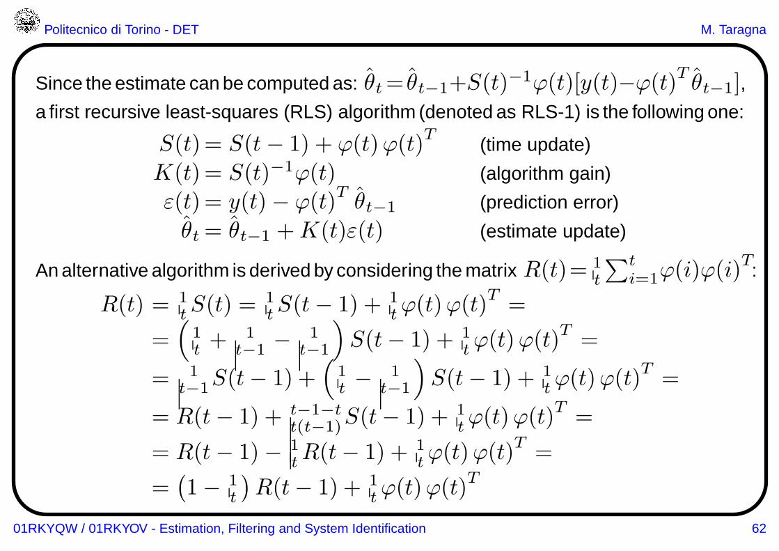
Since the estimate can be computed as: θt= θt−1+S(t)−1ϕ(t)[y(t)−ϕ(t)T θt−1],
a first recursive least-squares (RLS) algorithm (denoted as RLS-1) is the following one:
S(t)= S(t− 1) + ϕ(t)ϕ(t)T
(time update)
K(t)= S(t)−1ϕ(t) (algorithm gain)
ε(t)= y(t)− ϕ(t)T θt−1 (prediction error)
θt = θt−1 +K(t)ε(t) (estimate update)
An alternative algorithm is derived by considering the matrix R(t)= 1t
∑ti=1ϕ(i)ϕ(i)
T:
R(t) = 1tS(t) =
1tS(t− 1) + 1
tϕ(t)ϕ(t)T=
=(
1t +
1t−1 − 1
t−1
)
S(t− 1) + 1tϕ(t)ϕ(t)
T=
= 1t−1S(t− 1) +
(1t − 1
t−1
)
S(t− 1) + 1tϕ(t)ϕ(t)
T=
= R(t− 1) + t−1−tt(t−1)S(t− 1) + 1
tϕ(t)ϕ(t)T=
= R(t− 1)− 1tR(t− 1) + 1
tϕ(t)ϕ(t)T =
=(1− 1
t
)R(t− 1) + 1
tϕ(t)ϕ(t)T
01RKYQW / 01RKYOV - Estimation, Filtering and System Identification 62
Politecnico di Torino - DET M. Taragna
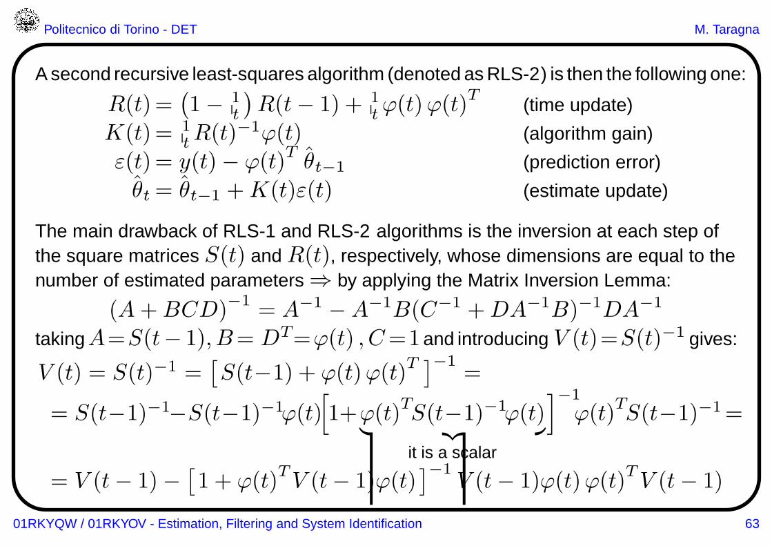
A second recursive least-squares algorithm (denoted as RLS-2) is then the following one:
R(t)=(1− 1
t
)R(t− 1) + 1
tϕ(t)ϕ(t)T
(time update)
K(t)= 1tR(t)
−1ϕ(t) (algorithm gain)
ε(t)= y(t)− ϕ(t)T θt−1 (prediction error)
θt = θt−1 +K(t)ε(t) (estimate update)
The main drawback of RLS-1 and RLS-2 algorithms is the inversion at each step ofthe square matrices S(t) and R(t), respectively, whose dimensions are equal to thenumber of estimated parameters ⇒ by applying the Matrix Inversion Lemma:
(A+BCD)−1 = A−1 − A−1B(C−1 +DA−1B)−1DA−1
takingA=S(t− 1), B= DT=ϕ(t) , C=1and introducing V (t)=S(t)−1 gives:
V (t) = S(t)−1 =[S(t−1) + ϕ(t)ϕ(t)
T ]−1=
= S(t−1)−1−S(t−1)−1ϕ(t)[
1+ϕ(t)TS(t−1)−1ϕ(t)
︸ ︷︷ ︸
it is a scalar
]−1
ϕ(t)TS(t−1)−1=
= V (t− 1)−[1 + ϕ(t)
TV (t− 1)ϕ(t)
]−1V (t− 1)ϕ(t)ϕ(t)
TV (t− 1)
01RKYQW / 01RKYOV - Estimation, Filtering and System Identification 63
Politecnico di Torino - DET M. Taragna
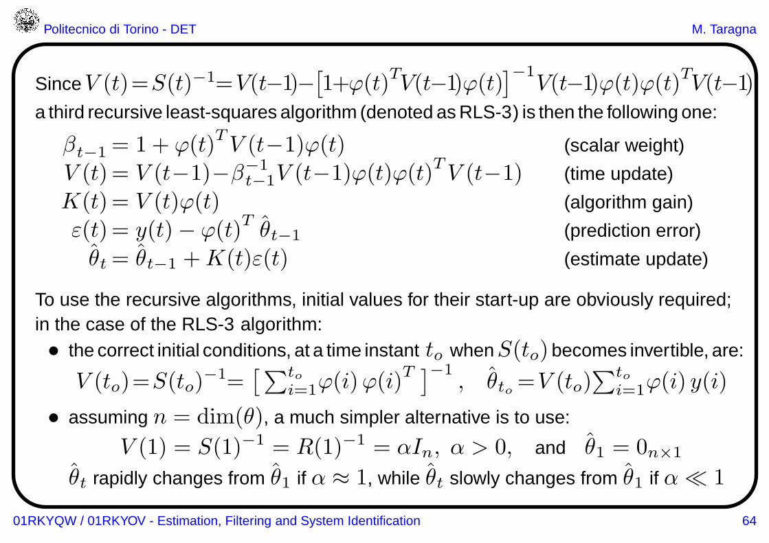
SinceV (t)=S(t)−1=V(t−1)−[1+ϕ(t)
TV(t−1)ϕ(t)
]−1V(t−1)ϕ(t)ϕ(t)TV(t−1)
a third recursive least-squares algorithm (denoted as RLS-3) is then the following one:
βt−1 = 1 + ϕ(t)TV (t−1)ϕ(t) (scalar weight)
V (t)= V (t−1)−β−1t−1V (t−1)ϕ(t)ϕ(t)
TV (t−1) (time update)
K(t)= V (t)ϕ(t) (algorithm gain)
ε(t)= y(t)− ϕ(t)Tθt−1 (prediction error)
θt = θt−1 +K(t)ε(t) (estimate update)
To use the recursive algorithms, initial values for their start-up are obviously required;in the case of the RLS-3 algorithm:• the correct initial conditions, at a time instant to whenS(to)becomes invertible, are:
V (to)=S(to)−1=
[∑toi=1ϕ(i)ϕ(i)
T ]−1, θto =V (to)
∑toi=1ϕ(i) y(i)
• assuming n = dim(θ), a much simpler alternative is to use:
V (1) = S(1)−1 = R(1)−1 = αIn, α > 0, and θ1 = 0n×1
θt rapidly changes from θ1 if α ≈ 1, while θt slowly changes from θ1 if α≪ 1
01RKYQW / 01RKYOV - Estimation, Filtering and System Identification 64
Politecnico di Torino - DET M. Taragna
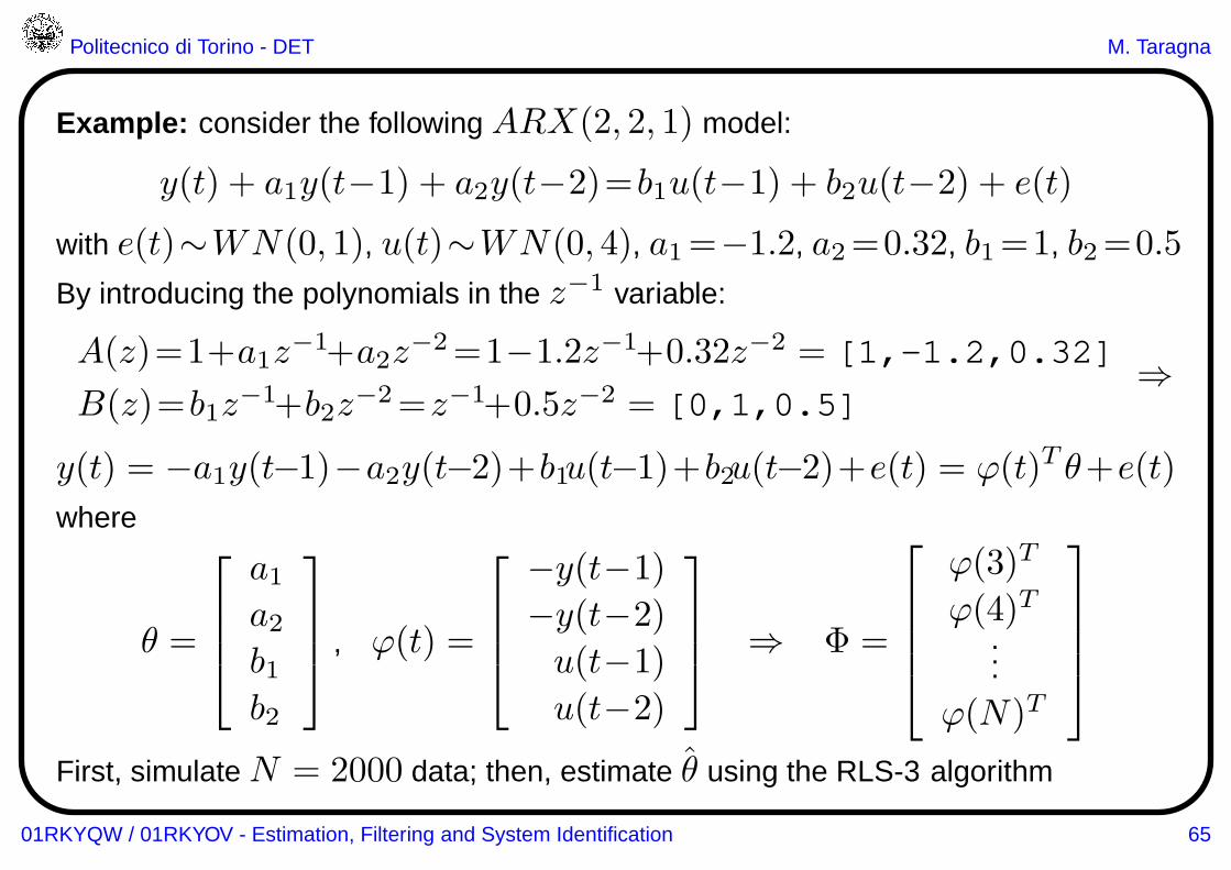
Example: consider the following ARX(2, 2, 1) model:
y(t) + a1y(t−1) + a2y(t−2)=b1u(t−1) + b2u(t−2) + e(t)
with e(t)∼WN(0, 1), u(t)∼WN(0, 4), a1=−1.2, a2=0.32, b1=1, b2=0.5
By introducing the polynomials in the z−1 variable:
A(z)=1+a1z−1+a2z
−2=1−1.2z−1+0.32z−2 = [1,-1.2,0.32]
B(z)=b1z−1+b2z
−2=z−1+0.5z−2 = [0,1,0.5]⇒
y(t) = −a1y(t−1)−a2y(t−2)+b1u(t−1)+b2u(t−2)+e(t) = ϕ(t)T θ+e(t)
where
θ =
a1a2b1b2
, ϕ(t) =
−y(t−1)
−y(t−2)
u(t−1)
u(t−2)
⇒ Φ =
ϕ(3)T
ϕ(4)T...
ϕ(N)T
First, simulate N = 2000 data; then, estimate θ using the RLS-3 algorithm
01RKYQW / 01RKYOV - Estimation, Filtering and System Identification 65
Politecnico di Torino - DET M. Taragna
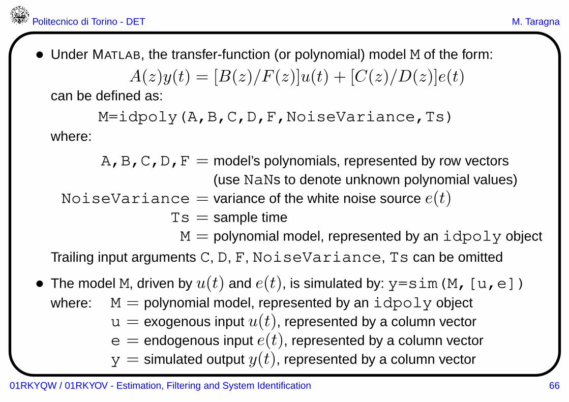
• Under MATLAB, the transfer-function (or polynomial) model M of the form:
A(z)y(t) = [B(z)/F (z)]u(t) + [C(z)/D(z)]e(t)can be defined as:
M=idpoly(A,B,C,D,F,NoiseVariance,Ts)
where:
A,B,C,D,F = model’s polynomials, represented by row vectors(use NaNs to denote unknown polynomial values)
NoiseVariance = variance of the white noise source e(t)Ts = sample timeM = polynomial model, represented by an idpoly object
Trailing input arguments C, D, F, NoiseVariance, Ts can be omitted
• The model M, driven by u(t) and e(t), is simulated by: y=sim(M,[u,e])where: M = polynomial model, represented by an idpoly object
u = exogenous input u(t), represented by a column vectore = endogenous input e(t), represented by a column vectory = simulated output y(t), represented by a column vector
01RKYQW / 01RKYOV - Estimation, Filtering and System Identification 66