Dipartimento di COSTRUZIONI E TRASPORTI -...
245
Sede Amministrativa: Università degli Studi di Padova Dipartimento di COSTRUZIONI E TRASPORTI SCUOLA DI DOTTORATO DI RICERCA IN: SCIENZE DELL’INGEGNERIA CIVILE ED AMBIENTALE CICLO XXII° IMPLEMENTATON AND VALIDATION OF ADVANCED CONSTITUTIVE MODELS FOR THE ANALYSIS OF HYDRO-THERMO-MECHANICAL INTERACTIONS IN GEO-ENVIRONMENTAL ENGENEERING PROBLEMS Direttore della Scuola: Ch.mo Prof. Stefano Lanzoni Supervisori: Ch.mo Prof. Bernhard Schrefler Dr. Lorenzo Sanavia Dottorando: Loris Luison
Transcript of Dipartimento di COSTRUZIONI E TRASPORTI -...

Sede Amministrativa: Università degli Studi di Padova
Dipartimento di COSTRUZIONI E TRASPORTI
SCUOLA DI DOTTORATO DI RICERCA IN: SCIENZE DELL’INGEGNERIA CIVILE ED
AMBIENTALE
CICLO XXII°
IMPLEMENTATON AND VALIDATION OF ADVANCED
CONSTITUTIVE MODELS FOR THE ANALYSIS OF
HYDRO-THERMO-MECHANICAL INTERACTIONS
IN GEO-ENVIRONMENTAL ENGENEERING PROBLEMS
Direttore della Scuola: Ch.mo Prof. Stefano Lanzoni
Supervisori: Ch.mo Prof. Bernhard Schrefler
Dr. Lorenzo Sanavia
Dottorando: Loris Luison


ABSTRACT
III
ABSTRACT
In recent years increasing interest in thermo-hydro-mechanical analysis of multiphase porous materials, i.e. saturated
and partially saturated porous materials, is observed, because of a wide spectrum of their engineering applications. An
area of particular interest is Environmental Geomechanics, where some challenging problems are of interest. Examples
are subsidence above gas reservoirs, injection of fluids into deep or superficial aquifers, long-term storage of carbon
dioxide, onset of flowslides and catastrophic landslides, nuclear and other hazardous waste disposal and stability of salt
marshes.
In all the aforementioned situations, the soil or rock need to be considered as multiphase porous medium in isothermal
or non-isothermal conditions, made of a solid phase and voids containing one or more fluids, in which the interaction
between all the components of the material cannot be neglected. In case of liquid and gaseous fluids, capillary effects
cannot be a priori neglected and also phase change for liquid water and its vapour can play a role.
This thesis aims to contribute to develop a general framework for the computational analysis of geo-environmental
engineering problems analysed as coupled multi-physics processes.
To this end, advanced constitutive models for isothermal and non-isothermal water saturated or unsaturated soils have
been implemented and numerically validated in the finite element code COMES-GEO.
In this THM model the porous medium is assumed to be a multiphase system where interstitial voids of the deforming
solid matrix may be filled with liquid water, water vapour and dry air or other gas. To handle this multiphase system, an
analytical multi-scale approach has been used by the general frame of averaging theories in deriving the governing
balance equations. These equations have been discretized in space and time by means of the finite element method for
a numerical solution.
These following advanced constitutive models for soil have been implemented:
1. ACMEG-T for water saturated clays in non isothermal condition;
2. ACMEG-TS for water saturated and partially saturated clays in non isothermal condition;
3. Pastor-Zienkiewicz for water saturated sands in isothermal condition;
4. Bolzon-Schrefler-Zienkiewicz for partially saturated sands in isothermal condition;
5. Bolzon-Schrefler for partially saturated sands in non isothermal condition.
Validation of the implemented models was performed by comparison between the F.E.M. results and the results
obtained by experimental tests or by the model driver. Three different tests were simulated: isotropic compression test,
oedometric compression test and triaxial compression test in different conditions of confining pressure, temperature and
suction and for different kind of soils. This comparison was done in cooperation with the research group of Prof. Lyesse
Laloui (EPFL of Lausanne) and the research group of the Prof. Manolo Pastor (UPM of Madrid).
Preliminary results concerning typical geo-environmental problems such as the thermo-hydro-mechanical behaviour of
deep nuclear waste disposal in a geological clay formation and the simulation of the subsidence above gas reservoirs
due to gas production close this present work, pointing out that with a sufficiently general thermo-hydro-mechanical
model the main couplings occurring in soils may be reproduced in a relevant manner and that very different situations
can be modelled without special assumptions.


SOMMARIO
V
SOMMARIO
Negli ultimi anni è aumentato notevolmente l’interesse per le analisi termo-idro-meccaniche sui mezzi porosi multifase,
che possono essere ad esempio analisi rivolte allo studio del comportamento dei terreni in parziale o totale saturazione,
per via della vasta gamma di applicazioni ingegneristiche che è possibile investigare. In particolare un’area di grande
interesse è rappresentata dai problemi di Geomeccanica Ambientale, dove si incontrano fenomeni di considerevole
importanza per la salvaguardia della società.
Alcuni esempi sono la subsidenza dovuta all’estrazione di gas dal sottosuolo, iniezione di fluidi dentro acquiferi profondi
o superficiali, stoccaggio a lungo termine di biossido di carbonio per la mitigazione del riscaldamento globale, innesco di
frane, stoccaggio di scorie nucleari o pericolose e la stabilità delle barene marine.
In tutte le situazioni menzionate, il terreno deve essere considerato come un mezzo poroso multifase, in condizioni
anche non isoterme, costituito da uno scheletro solido e da vuoti riempiti da uno o più fluidi dove le interazioni fra tutti i
costituenti non possono essere trascurate. In particolare nel caso di fluidi liquidi e gassosi, l’effetto delle pressioni
capillari non può essere tralasciato a priori, come anche il cambiamento di fase dell’acqua liquida e del vapor acqueo.
Lo scopo di questa tesi di dottorato è quello di contribuire a sviluppare uno strumento di carattere generale per l’analisi
computazionale di problemi ingegneristici di geomeccanica ambientale e questo è stato fatto mediante
l’implementazione e la validazione numerica di due modelli costitutivi avanzati nel codice agli elementi finiti COMES-
GEO.
Considerando il mezzo poroso multifase costituito da uno scheletro solido deformabile dove i vuoti possono essere
riempiti da acqua, vapore e aria secca (o un altro gas), tramite un approccio multiscala basato sulla teoria ibrida delle
miscele, con opportune procedure di media sono state derivate le equazioni di bilancio del modello. Queste equazioni
sono state poi discretizzate nello spazio e nel tempo per poter ottenere una soluzione numerica col metodo degli
elementi finiti.
I modelli costitutivi implementati sono i seguenti:
1. ACMEG-T per argille sature in condizioni non isoterme;
2. ACMEG-TS per argille parzialmente sature in condizioni non isoterme;
3. Pastor-Zienkiewicz per sabbie sature in condizioni isoterme;
4. Bolzon-Schrefler-Zienkiewicz per sabbie parzialmente sature in condizioni isoterme;
5. Bolzon-Schrefler per sabbie parzialmente sature in condizioni non isoterme.
La validazione dell’implementazione numerica dei modelli costitutivi è stata fatta tramite il confronto fra i risultati F.E.M. e
risultati sperimentali od ottenuti con il driver del modello. Le prove simulate sono di tre tipi: compressione isotropa,
compressione edometrica e compressione triassiale eseguite in differenti condizioni di pressione di confinamento,
temperatura e grado di saturazione per diversi tipi di materiale. Il lavoro di validazione è stato svolto in collaborazione col
gruppo di ricerca del Prof. Lesse Laloui (EPFL di Losanna) e quello del Prof. Manolo Pastor (UPM di Madrid).
Infine vengono mostrati alcuni risultati preliminari riguardanti due tipici problemi di Geomeccanica Ambientale, quali lo
stoccaggio di scorie nucleari e la subsidenza, per dimostrare come con un modello termo-idro-meccanico di carattere
sufficientemente generale, senza particolari assunzioni, sia possibile studiare un numero rilevante di problematiche
inerenti i problemi di accoppiamento nei terreni.


RINGRAZIAMENTI
VII
RINGRAZIAMENTI
Un ringraziamento particolare va al Dr. Lorenzo Sanavia prima per avermi proposto il dottorato e poi per avermi
indirizzato nel mondo della ricerca scientifica tramite varie vie. Non tralascio di ringraziarlo per l’attento e preciso
controllo fatto al presente lavoro.
Ringrazio Prof. Schrefler, senza il quale questo lavoro non sarebbe mai potuto essere stato fatto.
Parte di questo lavoro devo condividerlo anche con Mareva Passarotto per le analisi svolte assieme nella validazione e
per aver letto con pazienza le pagine successive.
Un ringraziamento anche a Raffaella Santagiuliana e Roberto Bortolotto per il contributo datomi nelle simulazioni.
Un aiuto fondamentale per poter completare questo lavoro è giunto dal Prof. Lyesse Laloui e dal Dr. Bertrand Francois
di Losanna con i quali il rapporto di cooperazione è iniziato già prima del dottorato.
Un grazie anche al Prof. Manolo Pastor e al Dr. Pablo Mira per il materiale che mi hanno fornito e senza il quale non
avrei potuto ottenere il risultato finale.
Volgo un ringraziamento particolare al Controrelatore di questa tesi, la Prof. Cristina Jommi di Milano, la quale, dopo
aver controllato con pazienza e profonda competenza il mio lavoro, ne ha dato un giudizio che mi ha infuso maggiore
sicurezza e consapevolezza.
Oltre che per il materiale fornitomi, ringrazio di cuore il Prof. Claudio Tamagnini per la disponibilità dimostratami e per la
compagnia offertami nelle occasioni in cui ci siamo incontrati.
Un ringraziamento infine va a tutto quello che ha rappresentato il dottorato in questi tre anni, alle persone incontrate nei
vari convegni e alle scuole di dottorato, a questo periodo della mia vita che ricorderò sempre con immenso piacere, per
gli infiniti stimoli che il mondo della ricerca ha saputo darmi e per le grandi persone che ne fanno parte e che ho potuto
conoscere o solo apprezzare.
Il mio ultimo pensiero infine va al mondo che sta al di fuori di quello che ho ringraziato finora, che indirettamente mi ha
permesso di fare tutto ciò con serenità e convinzione: Mareva, famiglia, amici.


CONTENTS
IX
CONTENTS
1 INTRODUCTION ..........................................................................................................................................3
2 MATHEMATICAL MODEL.........................................................................................................................11
2.1 INTRODUCTION ..........................................................................................................................................................11
2.2 AVERAGING PRINCIPLES ............................................................................................................................................11
2.2.1 AVERAGING PROCESS.............................................................................................................................................12
2.2.2 MICROSCOPIC BALANCE EQUATIONS........................................................................................................................15
2.2.3 MACROSCOPIC BALANCE EQUATIONS ......................................................................................................................15
2.3 MACROSCOPIC BALANCE EQUATIONS FOR A NON ISOTHERMAL PARTIALLY SATURATED POROUS MATERIAL..................17
2.3.1 KINEMATIC EQUATIONS...........................................................................................................................................18
2.3.2 MASS BALANCE EQUATIONS ....................................................................................................................................20
2.3.3 LINEAR MOMENTUM BALANCE EQUATION..................................................................................................................23
2.3.4 ANGULAR MOMENTUM BALANCE EQUATION ..............................................................................................................23
2.3.5 BALANCE OF ENERGY EQUATION .............................................................................................................................23
2.3.6 ENTROPY INEQUALITY .............................................................................................................................................24
2.4 CONSTITUTIVE EQUATIONS ........................................................................................................................................25
2.4.1 STRESS TENSOR IN THE FLUID PHASES ....................................................................................................................25
2.4.2 GASEOUS MIXTURE OF DRY AIR AND WATER VAPOUR................................................................................................26
2.4.3 SORPTION EQUILIBRIUM ..........................................................................................................................................26
2.4.4 CLAUSIUS-CLAPEYRON EQUATION...........................................................................................................................27
2.4.5 PORE SIZE DISTRIBUTION ........................................................................................................................................27
2.4.6 EQUATION OF STATE FOR WATER ............................................................................................................................28
2.4.7 DARCY'S LAW .........................................................................................................................................................28
2.4.8 FICK'S LAW.............................................................................................................................................................29
2.4.9 STRESS TENSOR IN THE SOLID PHASE AND TOTAL STRESS ........................................................................................30
2.4.10 SOLID DENSITY .....................................................................................................................................................31
2.4.11 FOURIER'S LAW ....................................................................................................................................................31
2.5 GENERAL FIELD EQUATIONS ......................................................................................................................................32
2.5.1 MASS BALANCE EQUATION ......................................................................................................................................32
2.5.2 LINEAR MOMENTUM BALANCE EQUATION..................................................................................................................35
2.5.3 ENERGY BALANCE EQUATION ..................................................................................................................................35
2.6 PHYSICAL APPROACH: EXTENDED BIOT'S THEORY......................................................................................................36
2.6.1 THE PHYSICAL MODEL .............................................................................................................................................36
2.6.2 CONSTITUTIVE EQUATIONS......................................................................................................................................40

CONTENTS
X
2.6.3 GOVERNING EQUATIONS ........................................................................................................................................ 42
2.7 QUASI STATIC CASE.................................................................................................................................................. 45
2.8 BOUNDARY AND INITIAL CONDITIONS ......................................................................................................................... 46
3 FEM MODEL ............................................................................................................................................. 51
3.1 THE CODE COMES-GEO ......................................................................................................................................... 51
3.1.1 INTRODUCTION ...................................................................................................................................................... 51
3.1.2 FINITE ELEMENT METHOD ...................................................................................................................................... 52
3.1.3 FINITE ELEMENT LIBRARY ...................................................................................................................................... 55
3.1.4 NUMERICAL INTEGRATION ...................................................................................................................................... 57
3.1.5 MATRIX SOLUTION PROCEDURE ............................................................................................................................. 58
3.1.6 CONVERGENCE AND ERROR ANALYSIS .................................................................................................................... 59
3.2 PLASTICITY IN SOILS ................................................................................................................................................. 60
3.2.1 CLASSICAL ELASTOPLASTICITY ............................................................................................................................... 61
3.2.2 MOHR-COULOMB YIELD SURFACE ........................................................................................................................... 64
3.2.3 CRITICAL STATE MODEL.......................................................................................................................................... 67
3.2.4 CORNERS OF YIELD AND POTENTIAL SURFACES...................................................................................................... 73
3.2.5 ADVANCED CONSTITUTIVE MODEL........................................................................................................................... 74
3.3 SIMULATION METHOD................................................................................................................................................ 74
3.3.1 INTRODUCTION ...................................................................................................................................................... 74
3.3.2 FINITE ELEMENTS USED FOR THE NUMERICAL VALIDATION........................................................................................ 74
3.3.3 TYPES OF TESTS.................................................................................................................................................... 75
3.3.4 REMARKS ON THE F.E.M. MODELLING APPROACH ................................................................................................... 79
4 THE THERMO-ELASTO-PLASTIC CONSTITUTIVE MODEL ACMEG-T................................................. 87
4.1 TEMPERATURE EFFECTS IN SOILS.............................................................................................................................. 87
4.1.1 THERMAL PROBLEM IN SOILS .................................................................................................................................. 87
4.1.2 THERMO-MECHANICAL BEHAVIOUR OF SOILS ........................................................................................................... 87
4.1.3 TEMPERATURE EFFECT ON PRECONSOLIDATION PRESSURE ..................................................................................... 91
4.1.4 TEMPERATURE EFFECTS ON SHEARING BEHAVIOUR ................................................................................................. 92
4.2 ACMEG-T MODEL ................................................................................................................................................... 93
4.2.1 INTRODUCTION ...................................................................................................................................................... 93
4.2.2 ACMEG MODEL .................................................................................................................................................... 94
4.3 ACMEG-T MODEL.................................................................................................................................................. 101
4.3.1 THERMO ELASTICITY ............................................................................................................................................ 101
4.3.2 THERMO PLASTICITY ............................................................................................................................................ 102

CONTENTS
XI
4.4 VALIDATION OF THE IMPLEMENTATION OF ACMEG-T MODEL IN COMES-GEO F.E. CODE ........................................105
4.4.1 INTRODUCTION .....................................................................................................................................................105
4.4.2 ELASTIC ISOTROPIC COMPRESSION IN NON-ISOTHERMAL CONDITION.......................................................................105
4.4.3 ELASTOPLASTIC ISOTROPIC COMPRESSION IN ISOTHERMAL CONDITION ...................................................................115
4.4.4 ELASTOPLASTIC TRIAXIAL COMPRESSION IN ISOTHERMAL CONDITION ......................................................................119
4.4.5 ELASTOPLASTIC ISOTROPIC COMPRESSION IN NON-ISOTHERMAL CONDITION ...........................................................120
4.5 A NON ISOTHERMAL CONSOLIDATION EXAMPLE ........................................................................................................123
5 THE THERMO-HYDRO-ELASTO-PLASTIC CONSTITUTIVE MODEL ACMEG-TS...............................131
5.1 PARTIAL SATURATION IN SOIL ..................................................................................................................................131
5.1.1 MECHANICAL BEHAVIOUR ......................................................................................................................................132
5.1.2 CONCLUSION........................................................................................................................................................135
5.2 ACMEG-TS MODEL................................................................................................................................................136
5.2.1 ISOTROPIC PLASTIC MECHANISM............................................................................................................................136
5.2.2 DEVIATORIC PLASTIC MECHANISM..........................................................................................................................137
5.2.3 COUPLING BETWEEN THE TWO PLASTIC MECHANISMS.............................................................................................137
5.3 WATER RETENTION CONSTITUTIVE PART ..................................................................................................................140
5.3.1 BROOKS AND COREY ............................................................................................................................................141
5.3.2 SAFAI AND PINDER ...............................................................................................................................................143
5.3.3 ACMEG-HYDRO ................................................................................................................................................144
5.3.4 COMPARISON .......................................................................................................................................................146
5.4 VALIDATION OF THE IMPLEMENTATION OF ACMEG-TS MODEL IN COMES-GEO F.E. CODE ......................................147
5.4.1 TRIAXIAL COMPRESSION TEST ...............................................................................................................................147
5.4.2 OEDOMETRIC COMPRESSION TESTS ......................................................................................................................153
6 THE GENERALIZED PLASTICITY MODEL FOR WATER SATURATED SANDS .................................165
6.1 GENERALIZED PLASTICITY .......................................................................................................................................165
6.2 PASTOR-ZIENKIEWICZ MODEL FOR SAND ..................................................................................................................168
6.2.1 PZ IN LOADING CONDITIONS ..................................................................................................................................171
6.2.2 PZ IN UNLOADING CONDITIONS ..............................................................................................................................177
6.2.3 LIQUEFACTION AND CYCLIC MOBILITY PHENOMENA .................................................................................................177
6.3 VALIDATION OF THE IMPLEMENTATION OF PZ MODEL IN COMES-GEO .....................................................................179
6.3.1 BANDING SAND .....................................................................................................................................................179
6.3.2 ADIGE SAND .........................................................................................................................................................183
6.3.3 DENSE SAND ........................................................................................................................................................187

CONTENTS
XII
7 THE GENERALIZED PLASTICITY MODEL FOR UNSATURATED SANDS ......................................... 191
7.1 INTRODUCTION ....................................................................................................................................................... 191
7.2 BSZ MODEL ........................................................................................................................................................... 192
7.3 BS MODEL ............................................................................................................................................................. 194
7.3.1 BS MODEL FOR SATURATED SOILS ....................................................................................................................... 195
7.3.2 BS MODEL FOR PARTIALLY SATURATED SOILS....................................................................................................... 196
7.4 VALIDATION OF THE IMPLEMENTATION OF THE BSZ MODEL IN THE F.E. CODE COMES-GEO..................................... 198
7.5 REMARKS............................................................................................................................................................... 203
8 APPLICATION TO GEO-ENVIRONMENTAL ENGINEERING PROBLEMS .......................................... 207
8.1 DEEP NUCLEAR WASTE DISPOSAL ........................................................................................................................... 207
8.1.1 INTRODUCTION .................................................................................................................................................... 207
8.1.2 SOURCE OF TEMPERATURE .................................................................................................................................. 208
8.1.3 MATERIAL PARAMETERS....................................................................................................................................... 210
8.1.4 INITIAL AND BOUNDARY CONDITIONS ..................................................................................................................... 211
8.1.5 MESH .................................................................................................................................................................. 213
8.1.6 SIMULATIONS....................................................................................................................................................... 213
8.1.7 RESULTS ............................................................................................................................................................. 214
8.1.8 FAILURE CONDITIONS ........................................................................................................................................... 219
8.2 SUBSIDENCE DUE TO GAS PRODUCTION................................................................................................................... 220
8.2.1 INTRODUCTION .................................................................................................................................................... 220
8.2.2 IDENTIFICATION OF PARAMETERS.......................................................................................................................... 220
8.2.3 RESERVOIR ANALYSIS .......................................................................................................................................... 225
9 CONCLUSIONS AND FUTURE DEVELOPMENTS................................................................................ 231


CHAPTER 1
3
1 INTRODUCTION
In recent years, increasing interest in thermo-hydro-mechanical analysis of multiphase porous materials, i.e. saturated
and partially saturated porous materials, is observed, because of a wide spectrum of their engineering applications. An
area of particular interest is Environmental Geomechanics [Vul02], [Sch01] and [S&D10], where some challenging
problems are of interest. Examples are subsidence above gas reservoirs with possible water injection to maintain
pressure (Figure 1.1), injection of other fluids into deep or superficial aquifers, long-term storage of carbon dioxide for
the mitigation of global warming, problems linked with soil failure such as the onset of flowslides and catastrophic
landslides (Figure 1.2), problems connected with nuclear and other hazardous waste disposal (Figure 1.3 and Figure
1.4), or groundwater, saturation response and stability of salt marshes subjected to both tide fluctuation and flooding
(Figure 1.5).
Figure 1.1: Scheme of extraction of gas and injection of CO2 [Sci09]
In all the aforementioned situations, the soil or rock need to be considered as multiphase porous medium in isothermal
or non-isothermal conditions, made of a solid phase and voids containing one or more fluids, in which the interaction
between all the components of the material cannot be neglected. In case of liquid and gaseous fluids, capillary effects
cannot be a priori neglected, and also phase change for liquid water and its vapour can play a role.

INTRODUCTION
4
Figure 1.2: Geologic section of Vajont slide before and after 9 October 1963 [R&S65] and [H&P85]
Figure 1.3: Repository tunnel with used fuel containers (Yucca tunnel, USA. NAI)
For enabling significant predictive simulations to be carried out, in particular for the long term behaviour, suitable
physical and mathematical models have to be developed and based on robust science; then, powerful and well validated

CHAPTER 1
5
software is necessary. To this end, coupled Thermo-Hydro-Mechanical (THM) finite element codes are of paramount
importance for simulation and analysis of geo-environmental engineering problems.
There are no general purpose codes available which handle all the above mentioned situations. There exist only a few
specialized codes which need however improvement.
Figure 1.4: Geological disposal of nuclear waste (M. Nuth, EPFL)
Figure 1.5: View of Venice lagoon marshes and view of a marsh border [Col08]
This thesis aims to contribute to develop a general framework for the computational analysis of geo-environmental
engineering problems analysed as coupled multi-physics processes.
To this end, advanced constitutive models for isothermal and non-isothermal water saturated or unsaturated soils have
been implemented and numerically validated in the finite element code COMES-GEO [G&S96], [L&S98], [S&P04],
[San06], [G&S09]. This code is based on an existing fully coupled Thermo-Hydro-Mechanical (THM) model developed
during years at the University of Padua [G&S96], [L&S98], [Sch02], [G&S09].
In this THM model the porous medium is assumed to be a multiphase system where interstitial voids of the deforming
solid matrix may be filled with liquid water, water vapour and dry air [L&S98] or other gas such as methane. To handle

INTRODUCTION
6
this multiphase system, an analytical multi-scale approach has been used by the general frame of averaging theories in
deriving the governing balance equations, [H&G79/1] and [H&G79/2]. These equations have been discretized in space
and time by means of the finite element method for a numerical solution [L&S98] and [Zie99].
In particular, the following advanced constitutive models for soil have been implemented:
1. ACMEG-T (Advanced Constitutive Model for Environmental Geomechanics – Thermal effects) for water
saturated clays in non isothermal condition, [M&L97] and [L&C08];
2. ACMEG-TS (Advanced Constitutive Model for Environmental Geomechanics – Thermal and Suction effects) for
water saturated and partially saturated clays in non isothermal condition [Fra08];
3. Pastor-Zienkiewicz for water saturated sands in isothermal condition, [Pas90] and [Zie99];
4. Bolzon-Schrefler-Zienkiewicz for partially saturated sands in isothermal condition [Bol96];
5. Bolzon-Schrefler for partially saturated sands in non isothermal condition [B&S05].
The first two models are based on the multi-mechanism elastoplasticity theory integrated by the bounding surface
theory, while the other three are based on the Generalized Plasticity theory.
The computational formulation of the elastoplastic algorithms developed for this thesis is of explicit type (Euler Forward
Method); for the tangent operator of the linearized system of equations [3.12] elastoplastic continuum tangent operator
has been computed.
Validation of the implemented models was performed by comparison between the F.E.M. results and the results
obtained by experimental tests or by the model driver. Three different tests were simulated: isotropic compression test,
oedometric compression test and triaxial compression test in different conditions of confining pressure, temperature and
suction and for different kind of soils.
This comparison was done in cooperation with:
1. the research group of Prof. Lyesse Laloui (EPFL of Lausanne) and in particular with the Dr. Bertrand Francois
for the ACMEG models;
2. the research group of the Prof. Manolo Pastor (UPM of Madrid) and in particular with the Dr. Pablo Mira for the
PZ model.
Validation of the implementation of BS model will be performed in the near future.
As further numerical validation a linear thermo elastic consolidation in fully saturated condition proposed originally by
Aboustit et al. [Abo85] and then by Lewis and Schrefler [L&S98] was analyzed. Then this case was extended to non liner
elasticity and [San08].
Preliminary results concerning typical geo-environmental problems such as the thermo-hydro-mechanical behaviour of
deep nuclear waste disposal in a geological clay formation and the simulation of the subsidence above gas reservoirs
due to gas production close this present work, pointing out that with a sufficiently general thermo-hydro-mechanical

CHAPTER 1
7
model the main couplings occurring in soils may be reproduced in a relevant manner and that very different situations
can be modelled without special assumptions.
This thesis is organized as follows:
After the introduction, CHAPTER 2 presents the governing equations of the T-H-M model following [L&S98].
Then CHAPTER 3 describes the space and time discretization of the mathematical model, a brief summary of the
elastoplasticity in soils and the F.E.M. modelling approach need in this work.
CHAPTER 4 to 7 present the constitutive models implemented in the finite element code COMES-GEO and the main
results concerning the validation of their FEM implementation.
CHAPTER 8 shows the preliminary results of the thermo-hydro-mechanical behaviour of deep nuclear waste disposal in
a geological clay formation and the simulation of the subsidence above gas reservoirs due to gas production.

INTRODUCTION
8
References
[Abo85] Aboustit B.L., Advani S.H. and Lee J.K. (1985). Variational principles and finite element simulations for
thermo-elastic consolidation. International Journal for Numerical and Analytical Methods in Geomechanics,
9: 49-69.
[B&S05] G. Bolzon, B.A. Schrefler. Thermal effects in partially saturated soils: a constitutive model. International
Journal for Numerical and Analytical Methods in Geomechanics, Vol. 29, pp. 861-877, 2005.
[Col08] Cola S., L. Sanavia, P. Simonini, B.A. Schrefler (2008) Coupled thermo-hydro-mechanical analysis of
Venice lagoon marshes. Water Resources Research, 44, W00C05. DOI:10.1029/2007WR006570.
[Fra08] François B. (2008). Thermo-Plasticity of Fine-Grained Soils at Various Saturation States: Application to
Nuclear Waste Disposal. PhD Thesis. École Polytechnique Fédérale De Lausanne. Suisse.
[G&S09] Gawin D., and L. Sanavia, (2009 – online first), Simulation of cavitation in water saturated porous media
considering effects of dissolved air, Transport in porous media. DOI: 10.1007/s11242-009-9391-4.
[G&S96] Gawin, D., and B.A. Schrefler, (1996), Thermo- hydro- mechanical analysis of partially saturated porous
materials, Engineering Computations, 13(7), 113-143.
[H&G79/1] Hassanizadeh, M. and Gray W.G., General conservation equations for multiphase systems: 1 Averaging
procedure, Adv. Water Resources, 2 (1979), 131-144.
[H&G79/2] Hassanizadeh, M. and Gray W.G., General conservation equations for multiphase systems: 2. Mass,
momenta, energy and entropy equations, Adv. Water Resources, 2(1979), 191-203.
[H&P85] Hendron, A.J. Patton, F.D.: The Vaiont slide, a geotechnical analysis based on new geologic observations
of the failure surface, Technical Report GL-85-5. Washington DC, Department of the Army US Corps of
Engineers vol. I, 1985.
[L&C08] Laloui L. and Cekerevac C. (2008). Non-isothermal plasticity model for cyclic behaviour of soils.
International Journal for Numerical and Analytical Methods in Geomechanics, 32(5): 437-460.
[L&S98] Lewis R.W. and Schrefler B.A. The Finite Element Method in the Static and Dynamic Deformation and
Consolidation of Porous Media. J. Wiley, Chichester 1998.
[M&L97] Modaressi H. and Laloui L. (1997). A thermo-viscoplastic constitutive model for clays. International Journal
for Numerical and Analytical Methods in Geomechanics, 21(5): 313–315.
[R&S65] Rossi D., Semenza E., Carte geologiche del versante settentrionale del Monte Toc e zone limitrofe, prima e
dopo il fenomeno di scivolamento del 9 ottobre 1963, Istituto di Geologia dell’Università di Padova, 1965.
[S&D10] B.A.Schrefler and Pierre Delage. Environmental Geomechanics. ISTE-Wiley, 2010.
[S&P04] Schrefler BA, F. Pesavento, Multiphase flow in deforming porous material., Computers and Geotechnics,
31 (2004), 237-250.
[San06] Sanavia, L., F. Pesavento, and B.A. Schrefler, (2006), Finite element analysis of non-isothermal multiphase
geomaterials with application to strain localization simulation, Computational Mechanics, 37(4), 331-348.
[San08] Sanavia L., François B., Bortolotto R., Luison L., Laloui L. (2008). Finite element modelling of thermo-
elasto-plastic water saturated porous materials. Journal of Theoretical and Applied Mechanics, 38, 1-2, pp
7-34.

CHAPTER 1
9
[Sch01] B.A. Schrefler. Environmental Geomechanics. CISM Courses and Lectures No 417, Springer Verlag Wien,
New York, 2001.
[Sch02] Schrefler, B.A., (2002), Mechanics and Thermodynamics of Saturated-Unsaturated Porous Materials and
Quantitative Solutions, Applied Mechanics Review, 55(4), 351-388.
[Sci09] Science. 25 september 2009 vol 325, issue 5948, pages 1585-1740
[Vul02] L. Vulliet, L. Laloui, B.A. Schrefler. Environmental Geomechanics – Monte Verità. EPFL Press, Lausanne,
2002.
[Zie99] Zienkiewicz, O.C., A. Chan, M. Pastor, B.A. Schrefler, and T. Shiomi, (1999) Computational Geomechanics
with special Reference to Earthquake Engineering. John Wiley & Sons, Chichester.


CHAPTER 2
11
2 MATHEMATICAL MODEL*
2.1 INTRODUCTION
In this chapter the governing equations for the full dynamic behaviour of a partially saturated porous medium are
developed. In particular, we consider here the voids filled with water and air. Today the description of multiphase
systems made of interpenetrating continuous bodies, such as porous media, is based either on the mixture theory
integrated by the concept of volume fractions, or on averaging theories and from a classical point of view on Biot's
theory. Since the averaging theories offer the possibilities of a better understanding of the microscopic situation and its
relation to the macroscopic one, which is, however, the natural domain of all continuum mechanical models, we use in
the following the averaging theory based on spatial averaging operators. Within this theory we make use of macroscopic
variables which correspond to real measurable quantities directly linked to laboratory practice, e.g. in soil mechanics. It
has to be pointed out that, under appropriate assumptions, the averaging theory yields the same equations as the
classical mixture theory, as shown in [deB91]. Care has to be taken, however, in the linear momentum balance equation
as explained in section 2.3.3.
For the reader mainly interested in the resulting governing equations and their numerical solution we derive these
equations again in section 2.6 using Biot's theory. This also permits us to establish a link between the classical,
phenomenological approach and the description of the real microscopic composition of the multiphase system.
Furthermore, it shows the essential correctness of Biot's findings.
Tensorial notation is used throughout this chapter.
2.2 AVERAGING PRINCIPLES
Here only a short summary of the principles necessary for the development of the governing equations is given. For a
full account of the averaging theories the reader is referred to References [deB91] and [B&D83]. Sections 2.2 and 2.3
follow, in particular, the work by Hassanizadeh and Gray [H&G79/1] and [Has86/2] and by de Boer et al. [deB91].
We introduce the following definitions:
1. microscopic level: we consider the real nonhomogeneous structure of the porous medium domain (Figure
2.1). The scale of inhomogeneity is of the order of magnitude of the dimensions of a pore or a grain, say d.
Attention is focussed on what happens at a mathematical point within a single phase and the field variables
describing the status of a phase are defined only at the points occupied by that phase. For the practical
* From Chapter 2: Mechanics of saturated and partially saturated porous media of: “Lewis R.W. and Schrefler B.A. The Finite
Element Method in the Static and Dynamic Deformation and Consolidation of Porous Media. J. Wiley, Chichester 1998”.

MATHEMATICAL MODEL
12
description of the processes taking place in a porous medium, this level is not useful since microscopic
quantities are generally not measurable. Only their average values are measurable.
2. macroscopic level: the real multiphase system that occupies the porous medium domain is replaced by a
model in which each phase is assumed to fill up the entire domain. This means that at every point all phases
are supposed present at the same time (overlapping continua). This is the level of interest of continuum
mechanics, where we investigate the continuous distribution of the constituents through a macroscopic control
space. At this level, we usually deal with homogeneous media, but nonhomogeneities may still be present, e.g.
strata. Their scale is of the order of magnitude comparable with the order of magnitude of the entire domain,
say L.
3. megascopic level: at this level the conditions are similar to those of the previously defined level. The difference
depends on the fact that some macroscopic inhomogeneities are eliminated by averaging and/or on the fact
that the mathematical model is stated in a domain which has less dimensions than the real domain, e.g. 2-D
problem with field values averaged over the thickness [B&C81] and [S&S89]. Typical applications of this level
are found in the simulation of land subsidence problems of regional scale.
Figure 2.1: Typical averaging volume dv of a porous media consisting of three constituents
2.2.1 Averaging process
We consider here a multiphase system occupying a total volume, V, and bounded by surface, A. The constituents
p=1,2,….,k have the partial volumes Vp. Each point of the total volume, V, is considered to be the centroid of a
representative elementary volume (R.E.V.) or average volume element, dv. The position of the centre of an R.E.V. in a
global coordinate system is described by position vector x while r indicates the position of a microscopic volume

CHAPTER 2
13
element, dvm, see Figure 2.1. The volume of constituent p within an R.E.V, called average volume element dvp, is
obtained by defining a phase distribution function, gp
≠∈∈=
απ
πγ
α
π
r 0
r 1),r(dvfor
dvfort [2.1]
where ξ+= xr
and the integration refers to the microscopic local coordinate system with its origin in x (Figure 2.1).
Similarly we write for the part of area dap of the R.E.V., occupied by constituent p
( ) ( ) mda
dattda ,rx, ∫= ππ γ [2.2]
where mda is the microscopic area element
The knowledge of dvp enables the introduction of the concept of volume fraction, hp, which is of paramount importance
in multiphase systems
( ) ( ) mdv
dvtdvdv
dvt ,
1, rx ∫== π
ππ γη [2.3]
with
11
=∑=
κ
π
πη [2.4]
In fact, as indicated under the heading "macroscopic level" in paragraph 2.2, substitute continua fill the entire domain
simultaneously, instead of the real fluids and the solid which each fill only part of it. These substitute continua have a
reduced density which is obtained through the volume fractions.
dvmin dv
Ave
rage
valu
e of
dvmax
Domain ofmicroscopic
inhomogeneity
Domain ofmacroscopic
inhomogeneity
Range for dv
Homogeneousmedium
Inhomogeneousmedium
Figure 2.2: Averaged value zzzz versus size of the average volume dv

MATHEMATICAL MODEL
14
In the following, averaged quantities are obtained by integrating (averaging) a microscopic quantity over the volume, dv,
or the area, da, of an R.E.V. A field of macroscopic variables results from this, where the average volume, dv, and the
average area, da, is associated with material points.
The importance in the choice of size of an R.E.V. is self evident. Average quantities have to be independent of the size
of the average volume and continuous in space and time. Thus an R.E.V. has to fulfil the following requirements:
- dv has to be small enough to be considered as infinitesimal, i.e. the partial derivatives appearing in the governing
equations must make sense and
-dv must be large enough, with respect to the heterogeneities of the material to give average quantities without
fluctuations depending on the size of the R.E.V., Figure 2.2.
To obtain meaningful average values, the characteristic length, l, of the average volume must satisfy the inequality
Lld <<<< [2.5]
where l is dependent on the specific material which constitutes the medium.
Some typical values of l are given in [L&C88]
l [mm]
metals 0.5
plastics 1.0
wood 10.0
Table 2.1: characteristic length l for some materials
The following average operators are now defined and applied to a function, z, which is a microscopic field variable.
Volume average operators
phase average
( ) ( ) ( ) mdv
dvttdv
t ,,1
, rrx π
πγζζ ∫= [2.6]
intrinsic phase average
( ) ( ) ( ) mdv
dvttdv
t ,,1
, rrx ππ
π
πγζζ ∫= [2.7]
From the definition of volume fraction [2.3] it follows that
( ) ( ) ( )ttt ,,, xxxπ
π
π
πζηζ = [2.8]
Mass average operator, with ( )t,rρ microscopic mass density as weighting function
( )( ) ( ) ( )
( ) ( )∫∫=
dv m
dv m
dvtt
dvtttt
,,
,,,,
rr
rrrx
π
ππ
γρ
γζρζ [2.9]
with constant microscopic mass density the following equation holds
CHAPTER 2
15
( ) ( ) ( )ttt
,,,
1xx
x
π
ππζζ
η= [2.10]
Area average operator
( ) ( ) ( ) mda
dattda
t , . ,1
, rnrx ππ
γζζ ∫= [2.11]
with n the outward normal unit vector of an area element dam and z has a tensorial nature.
In the following, averages of velocity, external body force, internal energy, external supply of heat, internal entropy,
external supply of entropy and total production of entropy are obtained through the mass average operator [H&G79/1].
2.2.2 Microscopic balance equations
We now consider the classical balance equations of continuum mechanics which are used to describe the microscopic
situation of any p phase. At the interfaces with other constituents, the material properties and thermodynamic quantities
may present step discontinuities.
For a generic conserved variable, y, the conservation equation within the p phase may be written as
( ) ( ) Gbir ρρρψρψ =−−+∂
∂ divdiv
t& [2.12]
where r& is the local value of the velocity field of the phase in a fixed point in space
i is the flux vector associated with y
b is the external supply of y
G is the is the net production of y
At the interface between two constituents p and a, the jump condition holds
( )[ ] ( )[ ] 0 . . =+−++− απ
α
παπ ρψρψ nirwnirw && [2.13]
where w is the velocity of the interface
παn is the unit normal vector pointing out of the p phase and into the a phase, with
αππα nn −= [2.14]
and π indicates that the preceding term [...] must be evaluated with respect to the p phase
No thermomechanical properties are attributed to these interfaces. This assumption does not exclude the possibility of
exchange of mass, momentum or energy between the constituents.
Moreover the local thermodynamic equilibrium hypothesis is assumed to hold because the time scale of the modelled
phenomena is substantially larger than the relaxation time required to reach equilibrium locally.
2.2.3 Macroscopic balance equations
Instead of deriving the macroscopic balance equation separately for each quantity to which the conservation law applies,
we derive it for the generic quantity, y, as in [deB91] and [B&D83] and specialise the law afterwards for specific

MATHEMATICAL MODEL
16
quantities: mass, linear momentum, angular momentum and energy. Note that the balance equations are written in a
material free manner. The constitutive equations are introduced successively.
A general, average macroscopic balance equation is obtained from the microscopic balance equation [2.12] by
multiplying it with the distribution function ( )t,rπγ and by integrating this product over the volume element, dv, and
over the total volume, V. In this elaboration of the balance equations, macroscopic quantities are obtained through the
previously defined averaging operators.
This averaging procedure yields that ([deB91] and [B&D83])
( ) ( )( ) ( ) dVdvtt
ttdvV dv
m ,,,1
∫ ∫
∂∂
rrr πγ
ψρ
(( ) ( ) )( ) ( ) dVdvttttdivdvV dv
m ,,, ,1
∫ ∫
+ rrrrr πγψρ &
( ) ( )∫ ∫
−V dv m dVdvttdiv
dv , ,
1rri πγ [2.15]
( ) ( )∫ ∫
−V dv m dVdvttdiv
dv , ,
1rri πγ
( ) ( ) ( ) dVttt
dvV dv ,, ,
1∫ ∫
− rrbr πγρ
( ) ( ) ( ) dVdvtttdvV dv
m ,,,1
∫ ∫
= rrGr πγρ
As suggested in References [H&G79/1], [H&G79/2], [H&G80/3] and [deB91], it is possible obtain the following form of
the general balance equation for the macroscopic thermodynamic property, πψ , associated with the phase
( ) ( ) ( ) ( ) ( )∫
+
∂∂
VdVtttdivtt
t,,v,,, xxxxx
ππ
π
π
πψρψρ
( ) ( ) ( ) ( )[ ] ( )∫ ∑∫
⋅−−
≠V
k
da m dVdatttttdv πα
παπα
ψρ ,,,,,1
rnrrrwrr &
( ) ( ) dVdattdvV
k
mda∫ ∑∫
⋅−≠πα
παπα
,, 1
rnri [2.16]
( ) ( ) ( )[ ] ( )∫ ∫
⋅−−
A da m dAdattttda
πππ γξψρ ,~
,,~
,,1
rnrxrri &
( ) ( ) ( ) ( )dVttdVttVV
,,,, xGxxbxπ
π
π
πρρ ∫∫ =−
or in more concise form
πππ
π
π
πψρψρ i v divdiv
tV−
+
∂∂
∫

CHAPTER 2
17
( ) dvdVebV
π
ππππ
πρρψρ GI ∫=
++− [2.17]
where πi is the flux vector associated with πψ
πb is the external supply of πψ
π
ρ is the volume average value of mass density
This last balance equation contains two further interaction terms, which describe chemical and physical exchanges.
Exchange of due to mechanical interactions between the constituents is given by
∑ ∫≠
⋅=πα
πα
π
π
παρda
mdadv
1
inI [2.18]
Phase change of a constituent or possible mass exchange between the constituent p and the other constituents a is
given by
( ) ( ) mdada
dvπα
παπ
ππαρψ
ρρψ nrw ⋅−= ∑∫
≠
&1
e [2.19]
2.3 MACROSCOPIC BALANCE EQUATIONS FOR A NON ISOTHERMAL
PARTIALLY SATURATED POROUS MATERIAL
In this section, the macroscopic balance equations for mass, linear momentum, angular momentum and energy
(enthalpy) are obtained and then specialised for a deforming porous material where heat transfer and flow of water
(liquid and vapour) and of dry air is taking place. The starting points are the microscopic balance equations [2.12],
where, for each constituent, the generic thermodynamic variable, z, is replaced by appropriate microscopic quantities,
suitable for a microscopic non polar material.
For the proper description of the nonisothermal unsaturated porous medium we need to take into account not only heat
conduction and vapour diffusion, but also heat convection, liquid water flow due to pressure gradients or capillary effects
and latent heat transfer due to water phase change (evaporation and condensation) inside the pores. Furthermore the
solid is deformable, resulting in coupling of the fluid, the solid and the thermal fields. All fluid phases are in contact with
the solid phase.
The constituents are assumed to be immiscible except for dry air and vapour, and chemically non reacting. Because of
the local thermodynamic equilibrium hypothesis, the temperatures of each constituent at a point in the multiphase
medium are taken to be equal. This does not mean that the temperature is uniform throughout the medium but only that
at each point one temperature is sufficient to characterize the state.
Momentum exchanges due to mechanical interaction are independent of the temperature gradient.
In the following, the stress is defined as tension positive for the solid phase, while pore pressure is defined as
compressive positive for the fluids.

MATHEMATICAL MODEL
18
It should be noticed that in this section the formulation is still material free, i.e. no specific assumptions for the material
behaviour have been introduced so far, except for the quite general ones, indicated above. For the development of the
macroscopic balance equations in the following sections, we still need to specify kinematics.
2.3.1 Kinematic Equations
As indicated in section 2.2, a multiphase medium can be described as the superposition of all p phases, whose material
points, Xn, can be thought of as occupying simultaneously each spatial point x in the actual configuration. The state of
motion of each phase is, however, described independently. Based on these assumptions, the kinematics of a
multiphase medium is dealt with next.
In a Lagrangian or material description of motion, the position of each material point, xp, at time, t, is function of its
placement in a chosen reference configuration, and of the current time, t
( ) ( ) ( ) ( ) 321321 ,, i,tXX,t,X,XXx,tXxx ti ===== ππππππ ff [2.20]
To have this mapping continuous and bijective at all times, the Jacobian, J, of this transformation must be non zero and
strictly positive, since it is equal to the determinant of the deformation gradient tensor,
( ) ππππ XF xF1
gradGrad ==−
[2.21]
Because of the non-singularity of the Lagrangian relationship [2.20], its inverse can be written and the Eulerian or spatial
description of motion follows
( )t,πππ xXX = [2.22]
It is also assumed that functions which describe the motion have continuous derivatives. If the path of the particle of the
p-phase is known, its velocity and acceleration are, in the material description
( )t
t∂
∂= , πππ Xx
V [2.23]
( )2
2 ,t
t∂
∂=ππ
π XxA [2.24]
The corresponding spatial expression can be obtained by introducing equation [2.22] into the above two equations. But,
if only the spatial description is given for the velocity field in the form
),( tπππ xvv = [2.25]
to evaluate its time derivative with material coordinates held constant, we introduce the description of motion of equation
[2.20] into the last equation. By applying the chain rule of differentiation, it follows
πππ
π vvv
a ⋅+∂
∂= gradt
[2.26]
The material time derivative of any differentiable function, ( )tf ,xπ , given in its spatial description and referring to a
moving particle of the phase is
ππππ
π
v ⋅+∂
∂= fgradt
fDtfD
[2.27]

CHAPTER 2
19
If superscript a is used for the operator DtD
απππ
α
v ⋅+∂
∂= fgradt
fDtfD
[2.28]
the time derivative is taken moving with the a-phase.
Subtraction of equation [2.27] from equation [2.28] yields the following relation
απππ
ππ
α
v ⋅+= fgradDtfD
DtfD
[2.29]
where
πααπ v v v −= [2.30]
is the velocity of the a phase with respect to the p phase. This velocity is called the diffusion velocity [H&G80/3].
The operator DtD
is a scalar operator and may be applied either to a vector quantity or a scalar quantity. If πf is a
vector property per unit volume referring to the p phase, the total time derivative of its integral over a volume, V, is given
by
( )∫∫∫
⊗+
∂∂=
+⋅+
∂∂=
vvvdVdiv
tVddivgrad
tdV
dtd
f
f ππ
πππππ
ππ vfvfvff [2.31]
For a scalar property, πf
( ) dVdivt
dVdtd
v v∫ ∫
+
∂∂= πππ
π vff
f [2.32]
In the above equations, velocities and accelerations of the p phase are considered as mass averaged quantities since
these are the quantities usually measured in a field situation or in laboratory practice. In porous media theory it is
customary to describe the motion of the fluid phases in terms of mass averaged velocities relative to the moving solid.
Their motion is described with reference to the actual configuration assumed by the solid skeleton. The velocities and
accelerations of each fluid particle can then be written with reference to the ones of corresponding solid points, once the
relative velocities are introduced. We specify the superscripts p now as s for soil, w for the liquid phase and g for the
gas phase (dry air plus vapour) and write for the relative velocities of water and gas phase respectively,
swws vvv −= [2.33]
sggs vvv −= [2.34]
Water and gas acceleration are given from [2.26], [2.28], [2.33] and [2.34] as
( ) wswssws
s
sw gradDt
Dvvv
vaa ⋅+++= [2.35]
( ) gsgssgs
s
sg gradDt
Dvvv
vaa ⋅+++= [2.36]

MATHEMATICAL MODEL
20
The deformation process of the solid skeleton can be described by the velocity gradient tensor, Ls, which, referred to
spatial co-ordinates, is given by [C&T92] and [Mol86]:
ssss grad WDvL +=≡ [2.37]
Its symmetric part Ds, is called the eulerian strain rate tensor, being related to pure straining while its skew-symmetric
component Ws is the spin tensor.
2.3.2 Mass balance equations
Figure 2.3: Schematic composition of soil
In the following, we identify the volume fractions, hp, of the constituents as
solid phase
ns −= 1η [2.38]
where dv
dvdvn
gw += is the porosity
water
ww Sn ⋅=η [2.39]
where gw
w
w dvdvdv
S+
= is the degree of water saturation
gas
gg Sn ⋅=η [2.40]
where gw
g
g dvdvdv
S+
= is the degree of gas saturation
It follows immediately that
1=+ gw SS [2.41]
2.3.2.1 Solid phase
In the microscopic situation, the variables for solid in equation [2.12] assume the following values

CHAPTER 2
21
0 ,0 ,0 ,1 ==== Gbiψ [2.42]
and the microscopic mass balance equation results in
( ) 0 =+∂∂
r&ρρ
divt
[2.43]
The averaged macroscopic solid mass balance equation is
( )ρρρρ s
s
s
ss evdiv
t=
+
∂∂
[2.44]
Where rs stands simply forπ
ρ , the phase averaged solid density and sv is the mass averaged solid velocity. The
same simplified notation will be used for the other constituents, once p is accordingly specified.
From [2.27] we have
s
sss
s
gradtDt
Dv ⋅+
∂∂= ρρρ
[2.45]
By introducing the latest in the previous equation we obtain
0v =+s
ss
s
divDt
Dρ
ρ [2.46]
By introducing intrinsic phase averaged densities through equation [2.8] we have finally
( ) ( ) 0v 11 =−+− ss
ss
divnDt
nDρ
ρ [2.47]
where the shorthand s
ss ρρ = has been introduced for the intrinsic phase averaged density.
2.3.2.2 Liquid phase: water
As for the solid phase we have:
( )ρρρρ w
w
w
ww edivt
v =
+
∂∂
[2.48]
( )ρρρρ w
w
w
ww
w
edivDt
D v =+ [2.49]
( ) meww
&−=ρρ [2.50]
Is the quantity of water per unit time and volume, lost through evaporation.
2.3.2.3 Gaseous phases: dry air and vapour
The gaseous phase here is a multi-component material, composed of two different species: dry air and vapour. These
species are miscible. We first write the mass balance equations for both species.
Their microscopic mass balance equations are again given by equation [2.43] if we neglect net production of mass of
each species, due to chemical reactions with the other species [Has86/2].

MATHEMATICAL MODEL
22
The macroscopic mass balance equation for dry air is given by equation [2.44] with appropriate super/subscripts and
with exchange term zero. We introduce intrinsic phase averaged densities and use super/subscript ga to indicate dry air.
Because the two species, dry air and vapour, are miscible, they have the same volume fraction nSg
( ) 0v =
+
∂∂ gaga
gga
g SndivSnt
ρρ [2.51]
Similarly we write for vapour, using super/subscript
( ) ( ) meSnSndivSnt
gwgwg
gwgwg
gwg
&==
+
∂∂
ρρρρ v [2.52]
We now derive the mass balance equation for the whole gaseous phase. This is obtained by summing the macroscopic
balance equations of the two species and using appropriate definitions for bulk properties of the gaseous phase
[Has86/2].
( ) mSndivSnt
ggg
gg
&=
+
∂∂
v ρρ [2.53]
with
gwgag ρρρ += [2.54]
and
gwgwgagagwgwgagag
gcc vvvvv +=
+= ρρ
ρ
1 [2.55]
where gc ρρππ = is the mass fraction of component p, subject to
gagwc , ,1 ==∑ ππ
π
[2.56]
We introduce further the macroscopic diffusive dispersive velocity, gwga,, =ππu defined as [Has86/1]
ggvvvu −==
πππ [2.57]
and subject to
∑ ==+π
ππρρρ 0uuu cggwgwgaga [2.58]
Transformation of [2.53] as in the case of the mass balance equation for the solid phase yields for gas
( )mdivSn
Dt
SnD ggg
gg
g
&=+ v
ρρ
[2.59]
With a proceedings similar to the earlier we obtained the following form of the mass balance equation for vapour
( ) ( ) mdivSnSndivSnDtD ggw
ggwgw
ggw
g
g
&=++ vu ρρρ [2.60]
We introduce now the diffusive-dispersive mass flux of component gw as [E&S64]
gwgwg
gwg Sn uJ ρ = [2.61]
and now we can write

CHAPTER 2
23
( ) mdivSndivSnDtD ggw
ggwg
gwg
g
&=++ vJ ρρ [2.62]
2.3.3 Linear momentum balance equation
Solid phase
( ) 0tagt =+−+ ss
sss
sdiv ˆ ρρ [2.63]
Liquid phase
( ) ( )[ ] 0treagt =++−+ πππ
πππ
π ρρρ ˆ &div [2.64]
where mdv
dvdv
π
π
π γρρ ∫= gg
1 is the external momentum supply, which we assume to be related to
gravitational effects
πππ
ππ vvv
va ⋅+== gradt∂∂& is the p-phase acceleration
The term
m
k
da m dadv
πα
παπ
πππαρ
nttI 1ˆ ⋅== ∑∫
≠ [2.65]
accounts for the exchange of momentum due to mechanical interaction of p-phase with the other a-phases.
2.3.4 Angular momentum balance equation
As indicated in section 2.3, all phases of the semi-saturated porous medium are considered microscopically non-polar.
The following microscopic variables are necessary for the balance equation [2.12] when angular momentum balance is
considered
0=
=
=
G
grb
tri
rr
x
x
x
m
&=ψ
[2.66]
With a proceedings similar to the earlier balance equation, or with an appropriate method chosen for the development of
the average angular momentum equation [deB91] and [H&G79/2], that for non-polar media, also at macroscopic level, it
can be shown that the partial stress tensor is symmetric
( )Tππ tt = [2.67]
and that the sum of the coupling vectors of angular momentum between the phases vanishes.
2.3.5 Balance of energy equation
For the energy balance, the following components must be taken into account in the generic microscopic balance
equation [2.12]:

MATHEMATICAL MODEL
24
0=
+
=21
G
rgb
qrti
rr
hm
&
&
&&
⋅=−
⋅+= Eψ
[2.68]
where ( )tE ,r is the specific intrinsic energy
( )t,rρ is the heat flux vector
( )th ,r is the intrinsic heat source
The energy balance equation can be written as follows
ππ
πππ
πππ
π
π ρρρ RdivhDtED +−+= qDt ~: [2.69]
where ( ) ( )[ ]πππππ
ππ ρρρρ QEeEeR +−= ˆ
The equilibrium between all the phases can be write
( ) ( ) ( ) 0ˆ21~ˆ =
+⋅+⋅+⋅+∑π
ππππππππππ ρρρρ QeeEe vtvvvr& [2.70]
and physically means that the total balance of energy exchange between all the phases is zero.
2.3.6 Entropy inequality
Exploitation of entropy inequality is a tool for developing constitutive equations in a systematic manner, leading to a
consistent thermodynamic description of the material behaviour at macroscale. The use of entropy inequality further
assures that the second law of thermodynamics is not violated. The procedure was proposed by Coleman and Noll
[C&N63]. It is, for instance, exploited in [S&W79], and by Gray and Hassanizzadeh [G&H91/1] for the development of
constitutive equations for unsaturated flow in dry or partially saturated soil, including interfacial phenomena.
The variables in the microscopic balance equation [2.12] are now
f=
=
G
b
i
s
Ø
=
=λψ
[2.71]
where l is the specific entropy
Ø is the entropy flux vector
s is an intrinsic entropy source
The net production f denotes an increase of entropy. The balance equation becomes then
( ) ( ) ρρρλρλ =−−+∂∂
sr Ødivdivt
& [2.72]
Starting from this last equation, lp, the averaged specific entropy of constituent p, and the entropy supply due to mass
exchange are determined for obtain the entropy inequality for the mixture
CHAPTER 2
25
( ) 011 ≥
−
++∑π
πππ
ππ
πππ
ππ
π ρλρρλ
ρ hdiveDt
DQQ
q [2.73]
where mdv
dvdv
π
π
π γρλρ
λ ∫= 1
qp the flux of entropy for unit of temperature
π
π
Q
h is the source of entropy for each phase
Again, this corresponds to the form used in the mixture theory as shown in [deB91].
Before further transformations of the macroscopic balance equations are made, we introduce the constitutive equations
for the constituents.
2.4 CONSTITUTIVE EQUATIONS
To complete the description of the mechanical behaviour, we now need to specify the constitutive equations. The
balance equations developed in the previous sections allows for the introduction of quite elaborate constitutive theories,
especially if the balance equations presented in the previous sections for the bulk material are extended to the
interfaces, as done by Gray and Hassanizadeh in [G&H91/1] and [G&H91/2] for the aspects concerning multiphase flow.
For the solid phase, second-grade material theories are also possible, where the gradients of relevant thermodynamic
properties, such as densities, are considered as independent variables [Ehl89]. However, since this book is application
oriented, i.e. we aim for the quantitative solution of real engineering problems, we make a different choice.
We select constitutive models which are based on quantities currently measurable in laboratory or field experiments, and
which have been extensively validated both with reference to known exact solutions and to experiments. Many of these
constitutive models correspond to linearization of more complex arguments.
We deal first with the properties of the fluid phases, and only briefly mention the solid phase here, because this is the
main aspect of this thesis and then this will be seen later.
2.4.1 Stress tensor in the fluid phases
By applying entropy inequality for the bulk material [H&G80/3] [G&H91/1], it can been shown that the stress tensor in the
fluid phases, is
It πππ η p−= [2.74]
where I is the identity tensor
pp is the macroscopic pressure of the p-phase
The volume fraction, hp, appears in equation [2.74] because tp is the force exerted on the fluid-phase per unit area of
multiphase medium. It should be noted that the stress vector in the fluid phase does not have any dissipating part. The

MATHEMATICAL MODEL
26
macroscopic effects of deviatoric stress components will be accounted for in linear momentum balance equations
through momentum exchange terms.
2.4.2 Gaseous mixture of dry air and water vapour
The moist air in the pore system is usually assumed to be a perfect mixture of two ideal gases, i.e. dry air and water
vapour. Hence the ideal gas law, relating the partial pressure, pgp, of species p, the mass concentration, rgp, of
species p in the gas phase and the absolute temperature, Q, is used.
The equations of state of a perfect gas, applied to dry air (ga), vapour (gw) and moist air (g) are
/
/
wgwgw
agaga
MRp
MRp
Q
Q
ρ
ρ
=
= [2.75]
11
1
−
+=
+=
+=
ag
ga
wg
gw
g
gwgag
gwgag
MMM
ppp
ρ
ρ
ρ
ρ
ρρρ
[2.76]
where Mp is the molar mass of constituent p
R is the universal gas constant
The second of equations [2.76] expresses Dalton's law [M&S93]. For the averaging process it is reminded that dry air,
vapour and moist air occupy the same volume fraction, nSg.
2.4.3 Sorption equilibrium
If an oven-dry porous medium is exposed to moist air, the weight of such solid increases because the moisture is
adsorbed on the inner surfaces of the pores starting with the finest ones. In the cases of interest here, the water is
usually present as a condensed liquid that, because of the surface tension, is separated from its vapour by a concave
meniscus (capillary water). There is then a relationship between the relative humidity, the water content (saturation) and
the capillary pressure in the pores.
The capillary pressure is defined as the pressure difference between the gas phase and the liquid phase, by the capillary
pressure equation
wgc ppp −= [2.77]
where pw is the pressure of the liquid-phase (water).
In [G&H91/2], it is shown that pc=pg-pw is not just a definition, but a derived relationship between two independent
quantities pc and pg-pw, at equilibrium.
For the relationship between the relative humidity (R.H.) and the capillary pressure in the pores, Kelvin-Laplace law is
assumed to be valid
==
QRMp
pp
HR ww
c
gws
gw
exp..ρ
[2.78]

CHAPTER 2
27
The water vapour saturation pressure, pgws, which is a function of the temperature only, can be obtained from the
Clausius-Clapeyron equation indicated below, or from empirical formulas such as the one proposed by Hyland and
Wexler [ASH93].
Assuming zero contact angle between the liquid phase and the solid phase, as is usually accepted for pore water, the
capillary pressure can be obtained through the Laplace equation from the pore radius, r
rpc σ2
= [2.79]
where s is the surface tension
These considerations are applicable if the water is present in the pores, as a condensed liquid (capillary region). When,
instead, the water is present as one or more molecular layers adsorbed on the surface of a solid because of the Van der
Waals and/or other interactions, the capillary pressure no longer has an obvious meaning, even if it can be retained,
referring to the broader concept of water potential or moisture stress. In such a case, a direct relationship between the
water content and the relative humidity is assumed to hold such as the BET equation. [ASH93].
2.4.4 Clausius-Clapeyron equation
As indicated above, this equation links the water vapour saturation pressure with temperature
( )
−−=
0
0 11 exp
∆Q
R
HMpp gwwgwsgws
[2.80]
where Q0 is a reference temperature
pgws is the water vapour saturation pressure at Q
pgws0 is the water vapour saturation pressure at Q0
DHgw is the specific enthalpy of evaporation
The equation is obtained from the second law of thermodynamics and is valid in the vicinity of Q0.
In the following, we denote T as the temperature difference above a reference value such that
0QQ-T = [2.81]
2.4.5 Pore size distribution
As it turns out from equations [2.78] and [2.79], the problem is to know the pore size distribution of the considered
porous medium, to relate the size of the largest pore filled (from which the capillary pressure depends) with the actual
water content. This relationship is obtained through experimental tests, usually centrifuge tests, sorption isotherm
measurements or mercury porosimetry.
The question is somewhat complex, because both the Laplace equation [2.79] and the Kelvin equation [2.78] are
obtained from a force equilibrium, evaluated in a cylindrical capillary tube, and the porous medium is considered as a
bundle of capillary tubes that do not intersect. The real porous media are more correctly represented as three-
dimensional networks of sites (or bodies) interconnected by narrower bonds (or throats) and then intrusion, extrusion,
adsorption and desorption are subjected to hysteresis. In this case, the actual value of capillary pressure can be only

MATHEMATICAL MODEL
28
interpreted as a measurable quantity describing complex adsorbed water-solid matrix interaction. The determination of
pore size distribution from sorption isotherms, results of centrifuge tests and mercury porosimetry should then be done
following the percolation theory approach, [B&S78].
The Rayleigh distribution or the log-normal distributions are often a good estimation of the pore size and often such
distribution can be bi-modal or multi-modal.
For soils, we need the Kelvin-Laplace equation [2.78], the Clausius-Clapeyron equation [2.80] and the capillary pressure
relationship
( )TpSS c ,ππ = [2.82]
which is directly obtained in laboratory.
In later chapters, where the constitutive models are introduced, will show different relationships for the pore size
distribution and one of them gives
( )vc TpSS εππ , ,= [2.83]
where vε is the volumetric strain
2.4.6 Equation of state for water
From the mass conservation in differential form
( )0
=Dt
VD www
ρ [2.84]
It can be possible to obtain
DtTD
DtpD
KDtD
w
w
ww
w
ww
wo βρ
ρ−= 11
[2.85]
where wβ is the thermal expansion coefficient
w
w CK
1=
wC is the compressibility coefficient
and where
ww
w
wo Kp11 =
∂∂ρ
ρ [2.86]
w
w
wo Tβ
ρ
ρ−=
∂∂1
[2.87]
2.4.7 Darcy's law
Darcy's law, generalized to allow for relative permeability
( )g πππ
πππ ρ
µη +−= pgrad
k rs k
v [2.88]

CHAPTER 2
29
where k is the permeability of the medium
m is the dynamic viscosity
krp the relative permeability, a dimensionless parameter varying from zero to one
is assumed valid for the transport of both water and gas in slow phenomena.
For each particular porous medium, the relations ( )wr Sk π are either predicted by models based on some more or less
realistic capillary assumption or experimentally determined in laboratory as well as field conditions. For typical curves of
relative permeabilities to water and air the reader is referred to Corey [Cor57].
The relative permeability goes to zero before the saturation reaches the value zero. The water saturation at which the
relative permeability goes to zero is termed the residual water saturation or displacement residual water saturation.
Relationships used in the following are e.g. those by Brooks and Corey [B&C66]
( )λ
λ32+= e
rw Sk [2.89]
λ
1
e
bc
S
pp =
[2.90]
where wc
wcwe S
SSS
−−=
1 is the effective saturation
Swc is the irreducible saturation
l the pore size distribution index
pb the bubbling pressure
2.4.8 Fick's law
Diffusive-dispersive mass flux is governed by Fick's law
−=
α
ππα
απα ρ
ρρ D J grad [2.91]
where παD is the effective dispersion tensor
p is diffusing phase
a is the phase in which diffusion takes place (a=w,g)
παD is a function of the tortuosity factor, which accounts for the tortuous nature of the pathway in soil; because of
mechanical dispersion, παD is also correlated with seepage velocity.
For dry air and water vapour (binary system) we have in particular, by the first of equations [2.76] and from the relation
gwgag ρρρ += that
gwgg
gw
gg
wag
g
ga
gg
waggag
pp
gradM
MM
pp
gradM
MM
J
J
−=
=
=
−=
D
D
2
2
ρ
ρ
[2.92]

MATHEMATICAL MODEL
30
It is worthwhile to emphasise that gas diffusion can take place even in the absence of a gas pressure gradient, i.e. when
its mass weighted velocity gv is zero.
2.4.9 Stress tensor in the solid phase and total stress
From the entropy inequality written in [G&H91/1] for unsaturated flow, including interfacial phenomena, it can be shown
that the stress vector in the solid phase is
( )( )sse
s pn Itt −−= 1 [2.93]
pressure in the solid phase is
gg
wws SpSpp += [2.94]
and
( ) sen tσ 1' −= [2.95]
is the effective stress tensor.
Introduction of [2.94] into [2.93] yields
( ) ( )[ ]gg
ww
se
s pSpSn 1 +−−= Itt [2.96]
The volume fraction (1-n) indicates that ts is the stress exerted on the solid phase per unit area of a multiphase medium.
The sum of [2.96] and of [2.74] written for gas and for water gives the total stress, s, acting on a unit area of a
multiphase medium
( ) ( )[ ] ( ) ( )gg
ww
se
gg
ww
gg
ww
se
gws pSpSnpnSpnSpSpSn +−−=−−+−−=++= ItIIIttttσ 11 [2.97]
This can be put in the usual soil mechanics form as
( )gg
ww pSpS +−′= Iσσ [2.98]
or
( )gg
ww pSpS ++=′ Iσσ [2.99]
From this last equation, it follows that the relationship between effective stress and total stress, in partially saturated
porous media, is no longer independent of the soil type because of the saturations, while in fully saturated soils, where
Sg=0 and Sw=1, the effective stress principle is unique for all soil types.
An expression of the effective stress principle was obtained by Bishop and Blight [B&B63] using a phenomenological
approach.
The effective stress is responsible for all major deformations in the skeleton and is linked to the strain rate tensor, Ds, by
means of a constitutive relationship
( )[ ]ssTDt
D0
'DDD −=σ
[2.100]
where
( )TpcsTT ,,',σDDD = [2.101]
is a fourth order tensor and s0D represents the increment of all other strains not directly associated with stress changes.

CHAPTER 2
31
2.4.10 Solid density
When considering the solid phase as compressible, a relationship for the material time derivative of the solid density can
be obtained from the mass conservation equation in differential form
( )0=
DtVD ss
s
ρ [2.102]
By assuming that the solid density is a function of ps, of temperature and of the first invariant of the effective stress, and
defining the Biot’s constant [B&W57] as
s
T
KK−= 1α [2.103]
we obtain
( ) ( ) ( )
−−−−−
−= s
s
s
ss
s
ss
s divDtTD
nDtpD
Kn
nDtD
v 11
111
ααβαρ
ρ [2.104]
where KT is the bulk modulus of the skeleton
Ks is the bulk modulus of the of the grain material
bs is the thermal expansion coefficient for the solid
In soils volumetric strain is relatively insignificant and can be ignored (a=1), but it is important in rock mechanics and in
concrete, where the compressibility of the solid phase is comparable to that of the skeleton.
2.4.11 Fourier's Law
A constitutive assumption for the heat flux is the generalized Fourier's Law
Tgradeff ~ χ−=q [2.105]
where ceff is the effective thermal conductivity tensor and is the heat flux of the multiphase medium
For isotropic media the generalized Fourier’s Law becomes the well known empirical Fourier's Law
Tgradq eff χ−= [2.106]
where ceff is the effective thermal conductivity
The effective thermal conductivity can be predicted theoretically as well as determined experimentally.
For porous building materials, for instance, the following linear relationship may be used, which represents with sufficient
accuracy the data by Bomberg and Shirtliffe [B&S78]
( )
−+= s
w
dryeff nnS
ρ
ρχχ
1 41
w
[2.107]

MATHEMATICAL MODEL
32
2.5 GENERAL FIELD EQUATIONS
The macroscopic balance laws are now transformed, and the constitutive equations introduced, to obtain the general
field equations, which will be used in the subsequent chapters. The averaging symbol, overbar, will be omitted in the
remainder of this book, because all quantities belong to the macroscopic situations.
2.5.1 Mass balance equation
2.5.1.1 Solid phase
The macroscopic mass balance equation for the solid phase [2.47], divided by rs is
( ) 0 11 =−+−− s
ss
s
s divnDt
nDDt
Dnv
ρ
ρ [2.108]
2.5.1.2 Liquid phase
Upon introduction of the relative velocity [2.33] and the material time derivative with respect to the moving solid [2.29]
equation [2.49] for liquid water becomes
( ) mdivgradDt
D wssww
wsw
s
&−=++⋅+ vv v
ρρρ
[2.109]
Introduction of intrinsic phase averaged densities with the appropriate volume fractions, use of vector identity written for
water and division by Swrw allows us to transform last equation into
( )w
w
swswww
w
w
s
w
ws
w
s
Sm
divnSndivSDt
SDSn
DtDn
DtnD
ρρ
ρ
ρ
ρ
&−=++++ v v
1
[2.110]
Summation with [2.108], to eliminate Dt
nDs
gives
( ) ( ) mS
SndivSDt
SDSn
DtDn
divDt
Dnw
w
wswww
w
w
s
w
ws
ws
ss
s&
1=v
1 v
1ρ
ρρ
ρ
ρ
ρ
ρ−++++−
[2.111]
Introduction of [2.85] and [2.104] for the material derivatives of the solid and water densities and of [2.94] gives
( ) ( )
( ) mS
SndivSDt
SDSn
DtTD
DtpD
Kndiv
DtTD
npSpSDtD
Kn
ww
wswww
w
w
s
w
s
w
ws
w
s
s
sggww
s
s
&
ρρ
ρ
βααβα
1v
1
1
v
−=++
−++−−+−
[2.112]
where pw, pg and T are independent variables
( )[ ]wswsw nnS ββαβ +−=

CHAPTER 2
33
For incompressible grains ( 1=α and 01 =
sK) this equation may be simplified as follows
( )w
wswww
w
ss
sws
w
ws
w
w mSndiv
DtSD
nDt
TDdivS
DtpD
KSn
ρρ
ρβ
&−=++−+ v
1 v
[2.113]
2.5.1.3 Gaseous phase
The mass balance equation for gas as a mixture of dry air and vapour is dealt with next.
In the same mode of the liquid phase, starting from [2.59] we obtain
( )
( ) ( ) mDtTD
SnnSdivDtSD
nSpK
n
Dt
MpMpR
DnS
divSDtpD
SK
nDtpD
SSK
n
g
s
gsgsg
ggw
s
gc
s
wgw
aga
s
ggs
g
gs
gs
ws
gws
&
ραβρ
ρ
α
ρα
αα
11
1
2
=−−+
+−−
+
+++−+−
v
v Q
[2.114]
where pw, pg and T are independent variables
For incompressible grains ( 1=α and 01 =
sK) this equation may be simplified as follows
( ) ( )
( )g
gsggg
wgw
aga
s
ggs
g
s
gsw
s
mSndiv
MpMpRDt
DnSdivS
DtTD
SnDtSD
n
ρρ
ρ
ρβ
&=+
+++−−−
v 1
1 v 1
Q [2.115]
For heat transfer analysis, in partially saturated porous media, it is more convenient to consider the mass balance
equation for dry air separately from that of vapour [Bag93] [Gaw95] and to sum the mass balance equations for both
water species, liquid water and water vapour. In this way, the mass rate of water evaporation, m& , disappears from the
mass balance equations. An evolution equation needed and this will be given by the energy balance equation. Note that,
in this way, no constitutive model for the mass rate of water evaporation is needed.
2.5.1.4 Gaseous phase: dry air
The mass balance equation for dry air is transformed in the following equation
0 )(
=++ ggag
gag
g
g
divnSdivDt
nSD ga
vJ ρρ
[2.116]
The resulting equation is divided by ggaSρ and summed with [2.108] we obtained
( ) ( ) 01
12
=−−+
+−−
++++−+−
DtTD
SnnSdivDtSD
nSpK
n
divDt
DnSdivS
DtpD
SK
nDtpD
SSK
n
s
gsgsga
ggaw
s
gc
s
gagga
gas
gags
g
gas
gs
ws
gws
αβρρ
α
ρ
ρ
ρα
αα
v
Jv
[2.117]

MATHEMATICAL MODEL
34
For incompressible solid grains this equation is simplified as
( ) ( )
( )g
gsggg
wgw
aga
s
g
gsg
s
gsw
s
mSndiv
MpMpRDt
DnSdivS
DtTD
SnDtSD
n
ρρ
ρ
ρβ
&=+
+++−−−
v 1
1 v 1
Q [2.118]
Introducing now the constitutive equations for rga and for gagJ to obtain
( )
( ) 0v 1
D 1
v 1
2=+
−
++−−−
gsgaggag
ga
gg
wagga
gaa
s
ga
gsg
s
gsw
s
Sndivpp
gradM
MMdiv
pR
MDtDnS
divSDt
TDSn
DtSD
n
ρρ
ρρ
ρβ
Q [2.119]
2.5.1.5 Gaseous phase: vapour
The way to derive the mass balance equation for vapour is identical to that of dry air and results, for the case of
incompressible solid grains, in
( )
( )gw
gsgwggwg
gw
gg
waggw
gww
s
gwgs
g
s
gsw
s
mSndiv
pp
gradM
MMdiv
pR
MDtDnS
divSDtTD
SnDtSD
n
ρρ
ρρ
ρ
ρβ
&=+
−
++−−−
v 1
D 1
v 1
2
Q [2.120]
This equation is now multiplied by rgw and added to the mass balance equation of liquid water, in turn multiplied by rw.
This sum gives the mass balance equation for the water species, liquid and vapour, without mass rate of water
evaporation as
( ) ( )
( ) ( ) 0v v
D
v
2
=++
−
++
++−−
wsww
gsgwg
g
gw
gg
waggww
s
g
ws
w
ww
sw
wg
gw
s
swgw
s
gww
SndivSndiv
pp
gradM
MMdivp
RM
DtD
nSDtpD
KSn
divSSDtTD
DtSD
n
ρρ
ρρ
ρρβρρ
Q [2.121]
where
( )( ) ww
wwwgw
gsswg SnSSn ρβρρββ 1 ++−= [2.122]
In these equations Darcy's law for the fluid velocities relative to the solid has still to be introduced. This law was
introduced in section Darcy's law2.4.7and will be derived again in its generalized form in the next section from the linear
momentum balance equations.

CHAPTER 2
35
2.5.2 Linear momentum balance equation
2.5.2.1 Fluids
A more suitable form for the linear momentum balance equation for the fluid-phases is now obtained by introducing
kinematic equations and constitutive relationships.
Equations [2.35] and [2.36] allow us to write for acceleration, ap
ππππ vvaaa gradsss ⋅++= [2.123]
where aps is the relative acceleration
Introduction in [2.64] of [2.123], [2.64], the momentum exchange term and of the intrinsic phase averaged density yields
( ) ( ) ( ) 0vRgrIvvaa =−++−⋅++− ssss peppdivgrad πππππππππππππππ ηηρηηρη & [2.124]
By neglecting the term dependent on the gradient of the fluid velocity, the effects of phase change and by applying a
vector identity, for the divergence of the stress tensor in the fluid-phase, we obtain the relative velocity of the fluid as
( ) ( )[ ]sss pgrad πππππππ ρηη aagRv −−+−=−1
[2.125]
[ ]) ( ss
rs pgrad
k ππππ
ππ ρµ
η aagk
v −−+−= [2.126]
Finally, neglecting the soil acceleration and the relative acceleration terms, it yields Darcy's law in the form [2.88]
( )g πππ
πππ ρ
µη +−= pgrad
k rs k
v [2.127]
Due to the simplifications introduced, this law is valid as a first approximation for slow flow of a macroscopically inviscid
fluid through a porous medium with incompressible grains.
2.5.2.2 Solid-phase
Taking into account equations [2.93], [2.94], [2.95], the linear momentum balance equation for the solid-phase becomes
( )( )[ ] ( ) ( ) 0 1 11 ' w =++−−−++−− wgggwswsssgg
ww nnpSpSndiv vRvRagIσ ηηρρ [2.128]
2.5.2.3 Multiphase medium
By summing the momentum balance equations, written for water and gas-phase respectively, with that of the solid phase
[2.128], by taking into account the definition of total stress, assuming continuity of stress at the fluid-solid interfaces and
by introducing the averaged density of the multiphase medium
( ) gg
ww
s SnSnn ρρρρ 1 ++−= [2.129]
we obtain the linear momentum balance equation for the whole multiphase medium
[ ] [ ] 0 + =+⋅+−⋅+−− gσvvavvaa ρρρρ divgradSngradSn ggsgsgg
wwswsww
s [2.130]
2.5.3 Energy balance equation
The energy balance equation for the single phase is
MATHEMATICAL MODEL
36
( ) πππ
ππ
πππ
ππ
ππ ρρρρρ HeRdivh
DtD
Cp −+−= q~Q
[2.131]
where ( )ππππ Q,pHH = is the specific enthalphy of the phase p
p
p
HC
∂∂=
π
ππ
Q is the specific heat at constant pressure
For the continuum multiphase, with the impose of thermodynamic equilibrium, the energy balance equation is
( ) ( ) ( ) vapeffgg
pgww
pweffp HmTgraddivTgradCCtT
C ∆&−=−⋅++ χρρρ vv∂
∂ [2.132]
where ( ) gpg
wpw
spseffp CCCC ρρρρ ++=
gwseff χχχχ ++=
wgwvap HHH −=∆
2.6 PHYSICAL APPROACH: EXTENDED BIOT'S THEORY
The governing equations, using Biot's theory [Bio41/1] [Bio41/2] [Bio55] [Bio56/1] [Bio56/2] [Bio63] are again derived but
extended to the case of non-isothermal two-phase flow in deforming porous media. This extension was made in
References [Sch95] [S&Z93] for the case of slow phenomena. Also, inertia forces are taken into account, as was done in
[Zie90] for the isothermal case with the air phase at atmospheric pressure.
The physical approach works directly with macroscopic variables. However, the distinction between a macroscopic and
microscopic domain is not so clear as in the previous sections, because macroscopic variables are sometimes directly
used in the microscopic domain.
For the sake of simplicity, small displacements are assumed for the solid phase. The governing equations in the form
needed for finite strain analysis are those of the previous section. For all queries regarding the assumed hypotheses the
interested reader is referred to the first part of this chapter.
2.6.1 The physical model
The voids of the skeleton are filled partly with water and partly with moist air (mixture of dry air and water vapour), which
is referred to as gas. The degree of water saturation Sw is given as the ratio between the pore space occupied by the
water and the total pore volume in a representative elementary volume element
gw
w
w dvdvdv
S+
= [2.133]
In the following equations the super or subscript p refers to the generic phase, p=s to the solid phase, p=w to water
and p=g to gas. The volume of the R.E.V. is dv, while the partial volumes are dvs, dvw and dvg. Their sum is dv while the
sum of the respective fluid volumes is dvT=dvw+dvg. The definition of the degree of gas saturation Sg is

CHAPTER 2
37
gw
g
g dvdvdv
S+
= [2.134]
and both degrees of saturation sum to one i.e.
1=+ gw SS [2.135]
The porosity n is defined as the ratio between the volume of voids and the total volume of the R.E.V.,
dvdvdv
ngw += [2.136]
As in the first part of this chapter, the stress is defined as tension positive for the solid phase, while pore pressure is
defined as compressive positive for fluids. The water pressure pw and the gas pressure pg are related through the
capillary pressure pc
wgc ppp −= [2.137]
The relation [2.137] is determined experimentally and usually shows hysteresis characteristics, which are ignored in this
case. Equation [2.137] is numerically inverted to obtain
( )pv
c TpSS εππ , ,= [2.138]
The constitutive law of the solid phase is introduced through the concept of effective stress
sp ' I+=σσ [2.139]
which stipulates that the main characteristics of the solid phase constitutive relation can be written in terms of s where
s is the total stress tensor, I the second order unit tensor and ps is the average pressure of both the water and air
surrounding the grains. In the case of immiscible two-phase flow we need a simple averaging technique for the
calculation of ps as described in section 2.2. Thus the modified effective stress principle may be obtained as stated
previously. The effective stress resulting from equation [2.138] is also referred to as Bishop's stress.
+== ∫ ∫∫
s fdv dv
mmmdv
dvdvdv
dvdv
1
1
σσσσ [2.140]
where σ is the macroscopic total stress tensor
For the fluid phases, the stress tensor is given by
πππ τσ p I−= [2.141]
where πσ is the intrinsic phase averaged stress tensor in the p phase
πτ is the shear stress
Under the assumption that the shear stress πτ is negligible in fluids, we obtain
( ) [ ]ww
gg
s pSpSnn +−−= 1 Iσσ [2.142]
The term in square brackets of equation [2.141] represents the intrinsically averaged (or mean) pressure ps of the fluid
phases i.e.
( )ww
gg
s pSpSp += [2.143]

MATHEMATICAL MODEL
38
This weighted pore pressures produce a stress state in the grains, but, for the moment, we assume these will not
undergo any deformation due to this stress, i.e. we introduce the hypothesis of incompressible grains. The deformation
of the solid skeleton, which depends on the effective stress, will be a function of the grain rearrangement only.
Equation [2.142] can be modified to
( )( ) ( ) ( )
s
ssss
ss
p
pnpnpn
pnn
1 1
1
I
III
I
−′=−−−+−=
−−=
σ
σ
σσ
[2.144]
where the overbar for the total stress has been omitted.
The stress tensor is split into two components: the pore pressure effect and the part which deforms the solid skeleton,
i.e. the effective stress. This latter is given by
( ) ( )ss pn 1 I+−=′ σσ [2.145]
Equation [2.144] results in a splitting of the stress tensor similar to that of Terzaghi's principle, which, in presence of
several fluid phases reads
( )gg
ww pSpS ++=′ Iσσ [2.146]
For greater generality, a corrective term known as Biot's constant, has to be introduced to account for the deformability
of the grains [B&W57]. Therefore a more general expression of the effective stress is assumed as follows
( )gg
ww pSpS +=′ ασσ + I [2.147]
where the corrective coefficient a will be determined in section 2.6.2. Note that this equation differs substantially from
the previous one: for the determination of a we need the constitutive equations of the solid phase. This effective stress
is indicated in this chapter by σ ′′ as in [Zie90].
Another, more intuitive way of deriving equation [2.145] follows Bishop [Bis59] and Skempton [Ske61]. Here the
microscopic and macroscopic aspects are somewhat mixed. We consider for this purpose the mean stresses, i.e.
3 ˆσ
σ tr= [2.148]
and
3 ˆσ
σ′
=′ tr [2.149]
If the pores (Figure 2.4) are filled with water and air, then due to the surface tension effect we have
gw pp < [2.150]
If the degree of saturation is relatively low, the water is present as menisci and the corresponding pressure acts over an
area c per unit gross area, [A&D56].
Consequently, the equivalent pore pressure is given by
( ) gw pp 1 χχ −+ [2.151]
and the equivalent pore pressure may be written as
( )wgg ppp −− χ [2.152]

CHAPTER 2
39
or
( ) ( )wgw ppp −−+ 1 χ [2.153]
For the fully saturated case, Bishop suggested the following expression for the mean effective stress σ ′ˆ
( )[ ]wgg ppp −−+=′ χσσ ˆˆ [2.154]
For the full stress tensor, this equation assumes the form
( )[ ]wgg ppp −−+=′ χσσ I [2.155]
das
da
pore waterpressure pw
pore airpressure pg
Figure 2.4: Contact area between two grains in the partially saturated case
The coefficient c is not the same as for problems involving shear strength and consolidation [Ske61]. For a given degree
of saturation the coefficient c must be determined experimentally for both types of problems.
In general the pressure is implied as being an absolute value, but in many soil mechanics problems relative pressures
are used and pg is often assumed to be equal to the atmospheric pressure. If this is the case and the atmospheric
pressure is assumed as the reference pressure then the effective stress principle becomes
wp χσσ I+=′ [2.156]
The comparison between [2.146] and [2.155] is noteworthy. The former may be written as a function of the degree of
saturation Sw
( )[ ]wgw
g ppSp −−− ' = Iσσ [2.157]
and coincides with equation [2.155] if wS=χ .
The coefficient c is related to the area of contact between solid and fluids, whereas the degrees of saturation Sp
depend on the volume occupied by the p phase. We define the volume fraction as
dvdvππη = [2.158]
and cross sectional area fraction as
dadaππα = [2.159]

MATHEMATICAL MODEL
40
For the case of microstructurally isotropic constituents, such that ap is independent of the orientation of the surface,
and assuming that
( )πππ ηαα = [2.160]
it can be shown that [Mor72]
ππ ηα = [2.161]
This conclusion coincides with the basic supposition of Delesse's law, see section 2.2.1.
If this assumption regarding the area and volume fraction is valid, then little difference exists between the definition of
Bishop's coefficient c and the degree of water saturation Sw. Bishop's equation [2.154] has been experimentally
validated by means of a triaxial tests carried out on soil samples [Ske61].
The assumption
wS=χ [2.162]
is acceptable for many materials as shown experimentally in [B&B63].
However, other expressions may also be used, e.g. by Gudehus for clay [Gud95]
( )SS −= 2χ [2.163]
If the solid phase is completely surrounded by a single wetting fluid phase, which is the only one in direct contact with
the porous medium, then Li and Zienkiewicz [L&Z92] use equation [2.156] with 1=χ , as in the case of a fully
saturated porous medium. This assumption is widely used when the two fluids are water and bitumen: only water is in
contact with the solid grains.
A new expression for the effective stress principle in fully saturated conditions only, involving four parameters, has been
proposed by Lade and de Boer [L&B96] and experimentally tested. This formulation, based on principles of mechanics is
valid for all types of materials. A distinction is made between the compressibilities of the grain particles and the skeleton
due to total stresses and pore pressures.
Two distinct expressions are then obtained for effective stresses in granular material and in solid rock with
interconnected pores respectively. For various special conditions these expressions become similar to the expressions
found in the literature, in particular to the expression used here with Biot's constant a. Lade and de Boer [L&B96]
conclude that Terzaghi's proposed effective stress principle works well for stress magnitudes encountered in most
geotechnical applications, but significant deviations occur at very high stresses.
2.6.2 Constitutive equations
For a full account of the constitutive relationships used the reader is referred to section 2.4, and only a few equations,
needed for the remaining part of this section, are recalled. In particular an expression for Biot's constant a is derived,
which was omitted in section 2.4.
The averaged pore pressure ps of the fluids occupying the void space induce a hydrostatic stress distribution in the solid
phase. The ensuing deformation is a purely volumetric strain
s
ssv K
p−=ε [2.164]

CHAPTER 2
41
where Ks is the averaged bulk modulus of the solid grains.
As stated previously, the effective stress causes all relevant deformation of the solid skeleton. The constitutive
relationship may be written as
( )[ ]°−−−=′ εεεεσ ddddd sv
c D T [2.165]
where σ ′d is the stress responsible for all deformations, except for the grain compressibility
εd represents the total strain of the solid
TD is the tangent constitutive tensor
( )εεσ &,,DD ′= TT [2.166]
( )dtgd c σε ′= accounts for the creep strain
odε represents all other strains in the solid skeleton not directly dependent on effective stress
A modified effective stress σ ′′ will now be introduced which will also account for grain compression. This allows the use
of Biot's constant a. Omitting, for brevity, cdε and odε we obtain
( )[ ] [ ] [ ]s
s
TTsvT K
dp Ddε =DdεdεDσd3
I+−=′ [2.167]
Consequently, the effective stress equation written in incremental form becomes
[ ] s
s
s
Ts dp
Kdp
Dσd dpσddσ III −+′′=−′=3
[2.168]
where σ ′′ represents the stress responsible for all deformation of the solid.
For the following developments we use indicial notation and the Kronecker Symbol d instead of the unit tensor I.
It can be immediately verified that equation [2.168] can be written as given by Zienkiewicz and Shiomi [Z&S85]
sij
sklmnklmnnmmnijij dp
KDdd δδδδδσσ
−−′′=
31
31
[2.169]
For an isotropic, elastic material
Tklmnklmn KE
D 921
3 =−
=υ
δδ [2.170]
where E is the Young's modulus
n is the Poisson's ratio
KT is the bulk modulus of the overall skeleton
Hence equation [2.169] can be written as
sijij
sij
s
Tijij dpdpd
KK
dd = 1 δασδσσ −′′
−−′′= [2.171]
where a is Biot's constant.
The resultant expression of the constitutive relationship is therefore
εσ dd T D=′′ [2.172]

MATHEMATICAL MODEL
42
The intrinsic pore pressure pp of the p fluid phase causes a purely volumetric strain of that phase, which is represented
by
π
ππε
Kp
v −= [2.173]
2.6.3 Governing equations
In the following a material coordinate system is employed for the solid phase and a spatial coordinate system for the fluid
phases; convective terms, unless specified otherwise, are neglected. Because of this choice of reference systems the
fluid velocities are conveniently referred to the solid phase by means of the relative velocities for water and gas
respectively
swws vvv −= [2.174]
sggs vvv −= [2.175]
and the accelerations, without convective terms, are
wssw aaa += [2.176]
gssg aaa += [2.177]
where aws is the acceleration of water relative to the solid phase and ags the relative acceleration of gas.
2.6.3.1 Linear momentum balance equation of the multiphase medium
The linear momentum balance equation for the multiphase system is the sum of the dynamics equations for the
individual constituents, but relative to the solid phase via equations [2.176] and [2.176]
0= gaaa ρσρρρ ++−−− divSnSn gsgg
wsww
s [2.178]
where
( ) gg
ww
s SnSnn ρρρρ 1 ++−= [2.179]
is the averaged density of the multiphase systems
rs is the intrinsic density of the solid phase, i.e. the density referred to the volume occupied by the solid phase
only, as opposed to the volume occupied by the multiphase system
rw is the intrinsic density of water
rg the intrinsic density of gas
g an acceleration usually related to gravitational effects
The linear momentum balance equation for each fluid phase yields the generalized form of Darcy's law, where the
dissipative terms arising in a multiphase flow system at the interfaces are taken into account through the relative
permeabilities
( )[ ]wssww
w
rwws
w pgradk
nS aagk
v −−+−= ρµ
[2.180]

CHAPTER 2
43
( )[ ]gssgg
g
rggs
g pgradk
nS aagk
v −−+−= ρµ
[2.181]
Where k is the intrinsic permeability
krw and krg the relative permeabilities of water and gas
mw and mg are the dynamic viscosities
The relative permeabilities vary between 0 and 1 and are a function of the degree of saturation; the dynamic viscosities
are temperature dependent. In the generalized form of Darcy's law for the gas phase the body forces are usually
neglected. The L.H.S. of equations [2.180] and [2.181] are multiplied by the volume fractions nSp because Darcy's law
is expressed in terms of volume averaged relative velocities. These are the velocities measured from experiment work.
2.6.3.2 Mass balance equations
The summation of mass balance equations of mass and fluid, with opportune arrangements and yields the so-called
continuity equation of the fluid phase i.e.
( ) ( )π
π
ππππ
π
π
π
π
π ρρ
ρ
ρ
ρ
ρ
ρ Sm
nSSt
SSnn
divt
n sss
s
&+=++++−
v1
t v
1∂
∂
∂
∂
∂
∂
[2.182]
We consider first the continuity equation for water. Introduction of the constitutive relationships for the time derivatives of
water density and solid density, of the pressure in the solid phase, and multiplication by Sw allows the continuity equation
for water and then with the introduction of Darcy's law and of the definition of capillary pressure yields
( )[ ]w
wssww
w
rww
w
wcw
ssw
sw
g
gws
w
w
ww
s
mpgrad
kdiv
tS
npSK
ntT
divSt
pSS
Kn
tp
KnS
SK
n
ρρ
µρ
ρ
αβ
ααα
&−=
−−+−+
∂∂
+−+
∂∂−
+∂
∂−+∂
∂
+−
aag k1
v 2
[2.183]
In the same way the continuity equation for gas is obtained
( )
( )[ ]g
gssgg
g
rgg
g
gg
ggs
ggs
sw
gc
s
g
gs
w
gws
mpgrad
kdiv
R
Mp
t
nSdivS
tT
Sn
tS
SpK
nn
tp
SK
nt
pSS
Kn
ρρ
µρ
ρ
ρααβ
ααα
&−=
−−+−+
∂∂++
∂∂−−
∂∂
−+−∂
∂−+∂
∂−
aag k1
v
2
Q [2.184]
2.6.3.3 Energy balance equation
By subtracting the kinetic energy from a global energy balance, the balance equation of thermal energy may be written
for constituent p as [Bir60]

MATHEMATICAL MODEL
44
( ) ( ) ππππππππππππ ρτρρ RgraddivpdivEdivEt
s+⋅+−−−=
∂∂
vvqv ~ [2.185]
where Ep is the specific internal energy
t is the deviatoric part of the stress tensor
µp the hydrostatic part of the stress tensor
The L.H.S. represents the rate of accumulation of internal energy in a control volume. The R.H.S. terms express
respectively the rate of internal energy change due to convection and to conduction, the reversible rate of internal energy
increase due to pressure, the irreversible rate of internal energy increase by viscous dissipation and the contribution of
heat sources.
In small strain the energy balance equation becomes
πππππππππππ
π ρτρρ RgraddivpdivEgradt
E +⋅+−−=⋅+∂
∂vvqv ~ [2.186]
The irreversible part of the internal energy increase by viscous dissipation is neglected in what follows. It is convenient to
express this equation in terms of temperature and heat capacity instead of internal energy [Bir60]. This is done through
the concept of enthalpy. Hence with sufficient accuracy for geomechanical applications the energy balance equation can
be rewritten as
ππππππ
ππ ρρ RdivTgradt
TCp +−=
⋅+
∂∂
qv ~ [2.187]
for p=s,w, which for the purpose of the energy balance only may be considered as incompressible, and
ggggg
gggg
gp Rpgrad
tp
divTgradt
TC ρρπ +⋅
∂∂+−=
⋅+
∂∂
+~ vqv [2.188]
where gpC is the specific heat at constant pressure
Some insignificant terms which are related to the mechanical work induced by density variations due to temperature
changes of the water and solid phases have been neglected.
Gas pressure changes are usually very slow and their gradients small in geomaterials, hence the time derivatives of gas
pressure, as well as the convective terms, are negligible with respect to other terms in equation [2.188]. Also, because
gas pressure changes are usually small when compared to atmospheric pressure, the specific heat at constant pressure
may be utilised instead of specific heat at constant volume.
A local equilibrium state is assumed to hold i.e.
TTTT gws === [2.189]
We also introduce the constitutive equation for heat fluxes, and add together equations [2.187] and [2.188], and
introduce the appropriate heat sources to obtain the following form of the energy balance equation
( ) ( ) ( ) vapeffgg
pgww
pw
effp HmTgraddivTgradCCtT
C ∆&−=−⋅++∂∂
χρρρ vv [2.190]
where vapH∆ is the latent heat of evaporation
The convective heat flux in the solid phase has been neglected.

CHAPTER 2
45
2.7 QUASI STATIC CASE
The relationship shown in 2.6.3 are now presented for quasi static conditions. In poor words, the equations are rewritten
by not taking into account the terms in which appear the acceleration, so is possible neglect the terms aw, as, aws, ag and
ags used in the relationship [2.176] and [2.177].
For this work of PhD, the equations used are those in quasi static condition.
2.7.1.1 Linear momentum balance equation of the multiphase medium
The equation [2.178] becomes
0= gρσ +div [2.191]
Where, as for the case seen in 2.6.3.1,
( ) gg
ww
s SnSnn ρρρρ 1 ++−= [2.192]
is the averaged density of the multiphase systems
rs is the intrinsic density of the solid phase
rw is the intrinsic density of water
rg the intrinsic density of gas
g is the gravity acceleration
2.7.1.2 Mass balance equations
The equations [2.183] and [2.184] becomes
[ ] 0g k1
v 2
=
+−+
∂∂
+−+
∂∂−
+∂
∂−+∂
∂
+−
ww
w
rww
w
wcw
ssw
sw
g
gws
w
w
ww
s
pgradk
div
tS
npSK
ntT
divSt
pSS
Kn
tp
KnS
SK
n
ρµ
ρρ
αβ
ααα
[2.193]
In the same way the continuity equation for gas is obtained
( )
[ ] 0g k1
v
2
=
+−+
∂∂++
∂∂−−
∂∂
−+−∂
∂−+∂
∂−
gg
g
rgg
g
gg
ggs
ggs
sw
gc
s
g
gs
w
gws
pgradk
div
R
Mp
t
nSdivS
tT
Sn
tS
SpK
nn
tp
SK
nt
pSS
Kn
ρµ
ρρ
ρααβ
ααα
Q [2.194]

MATHEMATICAL MODEL
46
2.7.1.3 Energy balance equation
The equation [2.190] write in 2.6.3.3 not change for the quasi static case but, using Darcy’ law, can be rewritten in a
complete mode as follow
( ) ( ) ( )[ ]
( )[ ] ( ) vapeffgg
g
ggp
g
wcgwp
w
effp
HmTgraddivTgradgpgradk
C
Tgradgpgradpgradk
CtT
C
∆&−=−⋅
+−
⋅
++−+
∂∂
k
k
r
w
rw
χρµ
ρ
ρµ
ρρ
[2.195]
2.7.1.4 Further developments of the model
The same equations see for this model, hence the linear momentum balance equation, the mass balance equations and
the energy balance equation, were developed by considering air dissolved in water by Gawin and Sanavia. For further
information, see [G&S10/1] and [G&S10/2].
2.8 BOUNDARY AND INITIAL CONDITIONS
For the model closure the initial and boundary conditions are needed. The initial conditions specify the full fields of
primary state variables at time t=t0, in the whole analysed domain B and on its boundary jB:
ug,c,T,BBB q =∂∪∂=∂ πππ [2.196]
BBTT
pp
pp
cc
gg
∂∪
=
=
=
=
on
0
0
0
0
uu
[2.197]
The boundary conditions (BCs) can be of Dirichlet’s type on jBp for t≥t0:
u
T
ccc
ggg
B
BTT
Bpp
Bpp
∂=
∂=
∂=
∂=
on ˆ
on ˆ
on ˆ
on ˆ
uu
[2.198]
or of Cauchy’s type (the mixed BCs) on jBqp for t≥t0:
( ) qg
gagad
gsgag B qvnS ∂=⋅+ onnJρ [2.199]
( ) ( ) qc
gwgwc
wgwgwd
gsgwg
wsww B qqvnSvnS ∂−++=⋅++ ∞ onρρβρρ nJ [2.200]
( ) ( ) ( ) qTc
wTeffvap
wsww B TTeTTqqgradTHnS ∂−+−++=⋅− ∞∞ on44
0σαχρ nv ∆ [2.201]
quB ∂=⋅ ontnσ [2.202]
where n(x,t) is the unit normal vector
qga(x,t) is the imposed fluxes of dry air

CHAPTER 2
47
qgw(x,t) is the imposed fluxes of vapour
qw(x,t) is the imposed fluxes of liquid water
qT(x,t) is the imposed imposed heat flux
t (x,t) is the imposed traction vector related to the total Cauchy stress tensor s(x,t)
gw∞ρ (x,t) is the mass concentration of water vapour
∞T (x,t) is the temperature in the far field of undisturbed gas phase
e(x,t) is the emissivity of the interface
0σ (x,t) is the Stefan-Boltzmann constant
bc(x,t) is the convective heat exchange coefficients
ac(x,t) is the convective mass exchange coefficients
The boundary conditions with only imposed fluxes are called Neumann’ BCs. The purely convective boundary conditions
for heat and moisture exchange are also called Robin’ BCs.

MATHEMATICAL MODEL
48
References
[A&D56] Aitchison, G.D., and Donald, I.B., Effective stress in unsaturated soils, Proc. 2nd Australia-New Zealand
Conf. Soil Mech., 1956, 192-199.
[ASH93] ASHRAE Handbook, Fundamentals Volume, ASHRAE, Atalanta, 1993.
[B&B63] Bishop, A.W. and Blight, G.E.: Some aspects of effective stress in saturated and partly saturated soils,
Géotechnique, 13(1963), 177-197.
[B&C66] Brooks, R.N., and Corey, A.T., Properties of porous media affecting fluid flow, J. Irrig. Drain. Div. Am. Soc.
Civ.Eng., 92(IR2) (1966), 61-68.
[B&C81] Bear, J. and Corapcioglu, Y., Mathematical model for regional land subsidence due to pumping. 2.
Integrated aquifer subsidence equation for vertical and horizontal displacements, Water Resour, Res.,
17(1981), 947-958.
[B&D83] Bear, J. and Bachmat, Y., Transport phenomena in porous media - Basic equations, from Fundamentals of
Transport Phenomena in Porous Media (Bear,J.and Corapcioglu, M. Y.. eds.), Nato ASI Series, Nijhoff,
Dordrecht, 1984, 5-61.
[B&S78] Bomberg M., Shirtliffe, C.J., Influence of moisture gradients on heat transfer through porous building
materials. Thermal transmission measurements of insulation, ASTM STP 660, R.P. Tye, ed., ASTM, 211-
233, 1978.
[B&W57] Biot, M.A., and Willis, P.G., The elastic coefficients of the theory of consolidation, J. Appl. Mech., 24, 594-
601, 1957.
[Bag93] Baggio, P., Bonacina, C., Strada, M., Trasporto di calore e di massa nel calcestruzzo cellullare. La
Termotecnica, 45(1993), 53-60.
[Bio41/1] Biot, M.A., General theory of three-dimensional consolidation, J. Appl. Phys., 12 (1941), 155-64.
[Bio41/2] Biot, M.A., Consolidation settlement under a rectangular load, J. Appl. Phys., 12 (1941), 426-30.
[Bio55] Biot, M.A., Theory of elasticity and consolidation for a porous anisotropo solid, J. Appl. Phys., 26 (1955),
182-5.
[Bio56/1] Biot, M.A., General solution of the equation of elasticity and consolidation for a porous material, J. Appl.
Mech., 23 (1956), 91-6.
[Bio56/2] Biot, M.A., Theory of deformation of a porous viscoelastic anisotropic soil, J. Appl. Phys., 27 (1956), 459-
67.
[Bio63] Biot, M.A., Theory of stability and consolidation of a porous medium under initial stress, J. Math. Mech., 12
(1963), 521-41.
[Bir60] Bird, R.B., Stewart, E.W., Lightfoot, E.N., Transport Phenomena, John Wiley & Sons, 1960.
[Bis59] Bishop, A.V., The principle of effective stress. Teknisk Ukeblad, 39 (1959), 859- 863.
[C&N63] Coleman, B.D., and Noll., W., The thermodynamics of elastic materials with heat conduction and viscosity,
Arch. Ration. Mech. Anal., 13(1963), 168-178.
[C&T92] Chen, W.F. and Tsui, Y., Limitations to the large strain theory, Int. J. Num. Meth. Eng., 33(1992), 101-114.
[Cor57] Corey, A.T., Measurement of water and air permeability in unsaturated soil, Soil Sci. Soc. Am. Proc., 21,1
(1957), 7-10.

CHAPTER 2
49
[deB91] de Boer, R., Ehlers, W., Kowalski S. and Plischka, J., Porous media, a survey of different approaches,
Forschungsbericht aus dem Fachbereich Bauwesen, 54, Universität-Gesamthochschule Essen, 1991.
[E&S64] Eringen A.C. and Suhubi, E.S., Nonlinear Theory of simple micro-elastic solids. Int. J. Engng. Sci. 2 (1964),
189-203.
[Ehl89] Ehlers, W., Poröse Medien, ein kontinuumsmechanisches Modell auf der Basis der Mischungstheory,
Forschungsbericht aus dem Fachbereich Bauwesen, 47, Universität Gesamthochschule Essen, 1989.
[G&H91/1] Gray, W.G., and Hassanizadeh S.M., Unsaturated flow theory including interfacial phenomena, Water
Resour, Res., Vol. 27(1991), 1855-1863.
[G&H91/2] Gray, W.G., and Hassanizadeh, S.M., Paradoxes and realities in unsaturated flow theory, Water Resour.
Res., Vol. 27(1991), 1847-1854.
[G&S10/1] Gawin D., L. Sanavia, Simulation of cavitation in water saturated porous media considering effects of
dissolved air. Transport in porous media, 81, 141-160 (2010). DOI: 10.1007/s11242-009-9391-4.
[G&S10/2] D. Gawin, Sanavia L., A unified approach to numerical modelling of fully and partially saturated porous
materials by considering air dissolved in water. Computer Modeling in Engineering & Sciences (Accepted).
[Gaw95] Gawin, D., Baggio, P. and Schrefler, B.A., Coupled heat, water and gas flow in deformable porous media,
I.J. Num. Methods in Fluids, 20 (1995), 969-987.
[Gud95] Gudehus, G., A comprehensive concept for non-saturated granular bodies, Proc. 1st Int. Conf.on
Unsaturated Soils, Paris 1995, Balkema Rotterdam.
[H&G79/1] Hassanizadeh, M. and Gray W.G., General conservation equations for multiphase systems: 1 Averaging
procedure, Adv. Water Resources, 2 (1979), 131-144.
[H&G79/2] Hassanizadeh, M. and Gray W.G., General conservation equations for multiphase systems: 2. Mass,
momenta, energy and entropy equations, Adv. Water Resources, 2(1979), 191-203.
[H&G80/3] Hassanizadeh, M. and Gray W.G., General conservation equations for multiphase systems: 3. Constitutive
theory for porous media flow, Adv. Water Resources, 3(1980), 25-40.
[Has86/1] Hassanizadeh, S.M., Derivation of basic equations of mass transport in porous media, Part. 1 Macroscopic
balance laws, Adv. Water Resources, Vol. 9(1986), 196-206.
[Has86/2] Hassanizadeh, S.M., Derivation of basic equations of mass transport in porous media, Part. 2 Generalized
Darcy's law and Fick's law, Adv. Water Resources, Vol. 9(1986), 207-222.
[L&B96] Lade, P.V., de Boer, R., The concept of effective stress for soil, concrete and rock, to appear in
Géotechnique, (1996).
[L&C88] Lemaitre, J. and Chaboche J.L., Mécanique des matériaux solides, Dunod, Paris 1988.
[L&S98] Lewis R.W. and Schrefler B.A. The Finite Element Method in the Static and Dynamic Deformation and
Consolidation of Porous Media. J. Wiley, Chichester 1998.
[L&Z92] Li, X., Zienkiewicz, O.C., Multiphase flow in deforming porous media and finite element solutions,
Computers and Structures, 45(1992), 211-227.
[M&S93] Moran, M.J. and Shapiro, H.N., Fundamentals of Engineering Thermodynamics, 2nd ed., J. Wiley, New
York, 1993.
[Mol86] Molenkamp, F., Limits to the Jaumann stress rate, Int. J. Num. Anal. Meth. Geomech., 10(1986), 151-176.

MATHEMATICAL MODEL
50
[Mor72] Morland, L.W., A simple constitutive theory for a fluid saturated porous solid, Journal Geophys. Res.
77(1972), 890-900.
[S&S89] Simoni, L. and Schrefler, B.A., F.E. solution of a vertically averaged model for regional land subsidence. Int.
J. Num. Meth. Eng., 27(1989), 215-230.
[S&W79] Sampaio, R. and Williams W.O., Thermodynamics of diffusing mixtures, Journal de Méchanique, Vol.
18(1979), 19-45.
[S&Z93] Schrefler, B.A., Zhan, X.Y., A fully coupled model for water flow and airflow in deformable porous media,
Water Resour. Res., 29(1993), 155-167.
[San05] L. Sanavia, F. Pesavento, B.A. Schrefler, Finite element analysis of non-isothermal multiphase
geomaterials with application to strain localization simulation, Computational Mechanics Vol. 466, (2005)
(DOI 10.1007/s00466 -005-0673-6).
[Sch95] Schrefler, B.A., Zhan, X., Simoni,L., A coupled model for water flow, airflow and heat flow in deformable
porous media, I.J. Heat and Fluid Flow, 5 (1995), 531-547.
[Ske61] Skempton, A.W., Effective stress in soil, concrete and rocks, from 'Pore Pressure and Suction in Soils',
Butterworths London 1961, 4-16.
[Z&S85] Zienkiewicz, O.C., and Shiomi, T., Dynamic behaviour of saturated porous media: the general Biot's
formulation and its numerical solution, Int. J. Num. Anal. Meth. Geom., 8(1985), 71-96.
[Zie90] Zienkiewicz, O.C., Xie, Y.M., Schrefler, B.A., Ledesma, A., Bicanic, N., Static and dynamic behaviour of
soils: a rational approach for quantitative solutions. II Semi-saturated problems. Proc. R. Soc. London. A
429 (1990), 311-321.

CHAPTER 3
51
3 FEM MODEL
3.1 THE CODE COMES-GEO
3.1.1 Introduction
The COMES-GEO code carries out the mechanical analysis of porous materials with interconnected pores in which the
flow of one or more fluid phases takes place.
The interactions between fluid and solid phases are taken into account. Geomaterials (soils, rocks, concrete), are the
most common examples of such porous media. The general purpose codes, currently available in the market, do not
deal with more than a single fluid phase. Therefore it is not possible to carry out realistic numerical studies of porous
materials structures in partially saturated conditions as:
1. seismic analysis of soil dams where in the upper part wide zones, containing pores filled with air and water, are
present;
2. stability analysis of soil slopes;
3. simulation of the subsidence phenomena in presence of gas extraction from deep reservoir. In this case water
and different gases are present in the pores. The gas reservoirs in the northern Adriatic Sea are an important
example in Italy.
The COMES-GEO code, developed by the University of Padua, is able to deal with these problems and also with many
others applications in the environmental geomechanics.
Due to the high frequency of earthquakes in Italy associated with the rich historical and architectural heritage potentially
affected by seismic or subsidence phenomena (Ravenna, Chioggia, Venezia), it is absolutely necessary to provide the
scientific community and the public institutions (as civil guard) with a COMES-GEO-like code.
Some simplified versions of the same code are already successfully applied to problems of environmental geomechanics
in Holland, United Kingdom and South Africa.
The problem unknowns are the following: temperature, capillary pressure, gas pressure and displacements. These data
allow the calculation of interesting derived outputs (saturation, stress-strain fields).
To reach the solution of the problem using the considered model, four balance equations are imposed (see chapter 2):
mass of the dry air, mass of the water species (both liquid water and vapour; phase change are considered); energy
conservation of the mixture and the linear momentum of the multiphase medium. They are completed by an appropriate
set of constitutive and state equations, as well as some thermodynamic relationships.
COMES-GEO allows any finite element analysis in plane strain and axialsymmetric conditions, using four node bilinear
elements or Serendipity eight node elements or Lagrange nine node elements.
The source is written in FORTRAN 90.

FEM MODEL
52
3.1.2 Finite Element Method
Numerical solution to the mathematical system presented in chapter 2, is done through use of the finite element method.
In what follows, we describe the particular method employed for the spatial discretization of the numerical system.
Specifically, we have elected to apply the Galerkin form of the method of weighted residuals (MWR) to produce an
integral representation of the basic conservation laws.
These relations are then specialized to finite element method.
For further information see Sanavia et al. [San05] and [San06].
3.1.2.1 Method of Weighted Residuals: discretization in space
To apply the MWR to the particular problem at hand, we assume that the region of interest W is divided into a number of
simply shaped regions, the finite elements, as shown in Figure 3.1.
y
x
Finite Element
Surface
Boundary Node
Figure 3.1: Schematic division in simply regions
Within each element, a set of nodal points is established at which the dependent variables pg, pc, T, ux and uy are
evaluated, where
1. pg is the pressure of gas (dry air, vapour or any other perfect gas) expressed in Pa
2. pc is the capillary pressure (or suction) expressed in Pa
3. T is the temperature expressed in K
4. ux and uy are the displacement expressed in m
For the purpose of developing the equations for these nodal unknowns, an individual element is separated from the
assemblage.
Within each element, it is assumed that the dependent variables can be expressed in terms of approximating function to
shape functions by:

CHAPTER 3
53
)()( tpNtp gpg = [3.1]
)()( tpNtp cpc = [3.2]
)()( tTNtT t= [3.3]
)()( tuNtu u= [3.4]
where the upper line indicates the nodal values. Substitution of the relations [3.1], [3.2], [3.2] and [3.4] into the partial
differential equations see in chapter 2, and boundary conditions, will result in a set of residual equations due to the
approximate nature of relations [3.1], [3.2], [3.2] and [3.4].
The MWR is then used to reduce the residual expression to zero in a weighted integral sense through the introduction of:
∫∫ =+ΓΩ
ΓΩ 0RNRN xxxx dd [3.5]
where uTppx ,,, cgT =
Nx are weighting or test functions
R is the residual for a field equation
Rx(b.c.) is the residual for the boundary condition
The integral or weak form of the heat and mass transfer equations (and of the other ones required to complete the
model), obtained by means of the Galerkin procedure (weighted residuals), [Z&T89] and [Z&T91], can be expressed in
matrix form as [Gaw96] and [S&G96]:
0fTCpCpCuC
0fTKpKpKuCTCpCpC
0fTKpKpKuCTCpCpC
0fTKpKpKuCTCpCpC
=++++
=+++++++
=+++++++
=+++++++
uuTcucguguu
TTTcTcgTgTuTTcTcgTg
ccTcccgcgcucTcccgcg
ggTcgcggggugTcgcggg
[3.6]
The above non-symmetric, non-linear and coupled system of ordinary differential equations can be rewritten in compact
form as:
( ) ( ) ( ) 0xfxxKxxC =++& [3.7]
where uTppx ,,, cgT =
and the non-linear (matrix) coefficients C(x), K(x) and f(x) are obtained by assembling the sub-matrices
indicated in [3.6].
3.1.2.2 Linearization: Discretization in time
Finite differences in time, [Z&T89] and [Z&T91], are used for the solution of the initial value problem over a finite time
step
nn ttt −= +1∆ [3.8]
where n is the time step number
Following the Generalised Trapezoidal Method as shown for instance in [L&S98], equation [3.7] is rewritten at time tn+1
using the relationships

FEM MODEL
54
tt
nn
n ∆Q
xxx −=∂
∂ +
+
1 [3.9]
( ) [ ]10 with1 1 ,nnn =+−= ++ QQQQ xxx [3.10]
where nx is the state vector at time tn
1+nx is the state vector at time tn+1
Dt is the time step length
thus obtaining
( ) ( ) ( )( ) 011 =−−−+= +++++ QQQ ∆∆-Q1∆Q nnnnnn ttt FxKCxKCxG [3.11]
Linearized analysis of accuracy and stability suggest the use of 2/1≥Q . In the present work implicit one-step time
integration has been performed ( 1=Q ).
After time integration the non-linear system of equation is linearized, thus obtaining the equations system that can be
solved numerically (in compact form)
( )iin n
in
1
1
11 +
+
−≅⋅∂
∂ ++ xGx
x
G
x
∆ [3.12]
where ( ) 11
++• i
n indicates the current iteration (i+1) in the current time step (n+1)
The Jacobian matrix has the following form
∂
∂
∂
∂
∂
∂
∂
∂
∂
∂
∂
∂
∂
∂
∂
∂
∂
∂
∂
∂
∂
∂
∂
∂
∂
∂
∂
∂
∂
∂
∂
∂
=∂
∂
+
uTpp
uTpp
uTpp
uTpp
x
G
x
uu
c
u
g
u
TT
c
T
g
T
cc
c
c
g
c
gg
c
g
g
g
GGGG
GGGG
GGGG
GGGG
in 1
[3.13]
Owing to the strong coupling between the mechanical, thermal and the pore fluids problem, a monolithic solution of
[3.12] is preferred using a Newton scheme, equation [3.8] can be rewritten as:
( )( ) ( )
( ) ( ) ( )
( ) ( ) ( )
++−−=
=
∂∂++
∂∂+
+
+−∂∂
++++
+
+++++
++++
ln
ln
ln
nlnl
n
ln
ln
ln
ln
ln
ln
lnn
ln
ln
t
t
1111
1
11111
1111
1
xfxxKxx
xC
xxfx
xKxxKx
xxCxxxCx
∆
∆
∆∆
[3.14]
Finally, the solution vector uTppx ,,, cgT = is then updated by the incremental relationship

CHAPTER 3
55
ln
ln
ln 11
11 ++
++ += xxx ∆ [3.15]
For the convergence and error analysis of the method applied here the interested reader is referred to [G&S96].
3.1.3 Finite Element Library
Three basic elements are utilized in the COMES-GEO code: the isoparametric quadrilateral elements with four and eight
node and the Serendipity nine node lagrangian element.
Within a particular element, the state’s variables are approximated using linear or quadratic shape functions.
)()( ttpp gpgg pN== [3.16]
)()( ttpp cpcc pN== [3.17]
)()( ttTT t TN== [3.18]
)()( ttuu uuN== [3.19]
Basic concepts of Finite Element Method element construction and isoparametric element formulation are thoroughly
described e.g. by Zienkiewicz [Z&T89].
The interpolation functions for any elements show below can be found in [Z&T89].
3.1.3.1 Four node quadrilateral elements
The basic four node quadrilateral element used in the code has 20 degrees of freedom as shown in Figure 3.2.
Figure 3.2: 4 node quadrilateral element
X
Y
Pg1,Pc1,T1,ux1,uy1 Pg2,Pc2,T2,ux2,uy2
Pg3,Pc3,T3,ux3,uy3 Pg4,Pc4,T4,ux4,uy4
ξ
η

FEM MODEL
56
3.1.3.2 Eight node quadrilateral elements
The basic four node quadrilateral element used in the code has 40 degrees of freedom as shown in Figure 3.3.
Figure 3.3: 8 node quadrilateral element
3.1.3.3 Nine node quadrilateral elements
The basic nine node quadrilateral element used in the code has 45 degrees of freedom as shown in Figure 3.4.
Figure 3.4: 9 node quadrilateral element
X
Y
Pg1,Pc1,T1,ux1,uy1 Pg3,Pc3,T3,ux3,uy3
Pg5,Pc5,T5,ux5,uy5
Pg7,Pc7,T7,ux7,uy7
ξ
η
Pg8,Pc8,T8,ux8,uy8
Pg6,Pc6,T6,ux6,uy6
Pg4,Pc4,T4,ux4,uy4
Pg2,Pc2,T2,ux2,uy2
X
Y
Pg1,Pc1,T1,ux1,uy1 Pg3,Pc3,T3,ux3,uy3
Pg5,Pc5,T5,ux5,uy5
Pg7,Pc7,T7,ux7,uy7
ξ
η
Pg8,Pc8,T8,ux8,uy8
Pg6,Pc6,T6,ux6,uy6
Pg4,Pc4,T4,ux4,uy4
Pg2,Pc2,T2,ux2,uy2
Pg9,Pc9,T9,ux9,uy9

CHAPTER 3
57
3.1.3.4 Mixed elements
The mixed element is shown in Figure 3.4 and is an element with eight node where the node on the corner are the only
with all the d.o.f..
Figure 3.5: Mixed element
3.1.4 Numerical Integration
As far as the numerical integration is concerned, the classical Gauss method is implemented in the code.
In this method the required matrix integrals, used in F.E.M., are in practice evaluated numerically using, for the case
treated here:
( ) ( )∑∫ =ji
jiij srdrdssr,
,, FF α [3.20]
The above formula is directly applicable to the calculation of matrices of rectangular elements, in which all integration
limits are -1 to +1. Thus we can apply the one-dimensional integration formulas successively in each direction. As the
analytical evaluation of multi-dimensional integrals, in this procedure, successively, the innermost integral is evaluated
by keeping the variables corresponding to the other integrals constant.
Therefore, we have for a two dimensional integral:
( ) ( )∑ ∫∫ ∫+
−
+
−
+
−
=i
ii dssrdrdssr1
1
1
1
1
1
,, FF α [3.21]
or
( ) ( )∑∫ ∫ =+
−
+
− jijiji srdrdssr
,
1
1
1
1
,, FF αα [3.22]
X
Y
Pg1,Pc1,T1,ux1,uy1 Pg3,Pc3,T3,ux3,uy3
Pg5,Pc5,T5,ux5,uy5
Pg7,Pc7,T7,ux7,uy7
ξ
η
ux8,uy8
ux6,uy6
ux4,uy4
ux2,uy2
Pg9,Pc9,T9,ux9,uy9

FEM MODEL
58
In COMES-GEO code we have the possibility to use different orders of integration. The possible numerical integration
are presented in the following table, but for the kind of problems resolved using COMES-GEO, fully coupled and strongly
non-linear, it is suggest to use eight node quadrilateral elements with a 3×3 numerical integration.
Type of element Order of integration Note
2×2
There is not stabilization in case of reduced
interpolation (i.e. with 1 gauss point)
3×3 also 2×2 is available
Table 3.1: Type of element and order of integration
3.1.5 Matrix Solution Procedure
When the solution algorithms of the theory section are applied to a given iteration or time step, the general result is a
matrix equation of the form:
Ax = b
In the problem considered here the A matrix is large (e.g. several thousand equations), sparse, banded, and generally
unsymmetric.
The solution of the equations system [3.14] may be approached by a direct method.
The solution procedure used in COMES-GEO is a form of Gauss elimination developed by Irons, called frontal solution
method. In particular it is a super fast frontal elimination routine using diagonal pivoting reduced fill-in version which
assembles the contribution of each element to form the global stiffness matrix and global load vector and to solve the
resulting set of simultaneous equations by Gaussian direct elimination [Bia03].
The main feature of the frontal solution technique is that it assembles the equations and eliminates the variables at the
same time.
In fact the basic premise of the frontal method is that the process of assembling the system matrix A, from the individual
element matrices and the reduction of A by standard Gauss elimination may be efficiently intertwined.
In processing each element in sequence, the frontal procedure passes through the following steps:
1. assembly of element equations into global matrix A;
2. check each equation in the assembled system to determine if all contributions to this equation have been made;

CHAPTER 3
59
3. condense from the system (by Gaussian elimination) the equations for all degrees of freedom that have been
completely assembled;
4. return to step 1. for the next element.
By combining the assembly and reduction process, computer storage is effectively minimized since only the currently
“active” (i.e. incompletely assembled) degrees of freedom are retained in the core storage.
Following the reduction of the matrix A to an upper triangular form, a back-substitution algorithm completes the solution
process for the vector x.
Since the frontal method is structured around the individual element, it is especially adaptable for general purpose code
with an element library.
The processing of higher order elements (e.g. quadratic basis functions) is also handled efficiently by frontal method.
The frontal procedure in COMES-GEO employs diagonal pivoting reduced fill-in. In our case it is a total pivoting which is
related to the numerical stability in a strong manner, and works on rows and columns to find the “pivot”. The pivoting
technique allows improving the convergence of the numerical system.
3.1.6 Convergence and error analysis
The discretization in space of the balance equations (and of the other ones required to complete the model) with the
standard Galerkin method (weighted residuals), results in a non-symmetric, non-linear and coupled system of ordinary
differential equations as shown in the section 3.1.2:
( ) ( ) ( ) 0xfxxKxxC =++& [3.23]
where uTppx ,,, cgT =
and the non-linear (matrix) coefficients C(x), K(x) and f(x) are obtained by assembling the sub-matrices indicated in
[3.6].
We assume consistency and convergence of the finite element discretization in space.
The time discretization is accomplished through a fully implicit finite difference scheme (backward difference)
0FBxAx =−−+ nn 1 [3.24]
where
( ) ( ) tnn ∆11 ++ += xKxCA [3.25]
( )1+= nxCB [3.26]
( ) tn ∆1+−= xfF [3.27]
where n is the time step number
Dt the time step length
We focus our attention on the global error
Lnn
Ln 111
~~+++ −= xxe [3.28]
where 1~
+nx is the exact solution of the equation [3.24]
L is the number of performed iterations for the time step n+1

FEM MODEL
60
To simplify calculations, we assume that there are not round-off errors generated by the algorithm, except those
introduced by the initial values at time t0.
If we replace 1+nx and nx in equation [3.24] by the corresponding exact values, we obtain:
11~~~
++ ++= nnn rFxBxA [3.29]
where rn+1 is the local truncation error of equation [3.24]
The calculated numerical solution Ln 1+x satisfies equation [3.24], so we can subtract equation [3.24] written for L
n 1+x
and Lnx respectively from the equation [3.29].
This results in:
11 ++ += nLn
Ln rBeAe [3.30]
Neither symmetry not positive definiteness of the matrices is assumed here.
By a recursive application for the index n, we have from equation [3.29] that:
( ) ( ) ( )( ) ( ) ( ) 11
111
1
1
01
1001
11
11
++−
−−−
−+−
−
=+
−−+
−+
+⋅⋅⋅
⋅⋅⋅+⋅⋅⋅= ∑
nnknknkn
n
knn
Ln
rArAAB
ABeABABe [3.31]
The total error Ln 1+e is influenced by the local truncation error rk, being k ≤ n+1 and by the initial round-off error 0
0e
made at the starting step, because then for n=0 and L=0
000
00
~ xxe −= [3.32]
where 00~ xx = is the exact solution of the equation [3.24]
Thus
n∀<− 11BA [3.33]
where ⋅ is the spectral norm
is the sufficient stability condition for applied solution procedure.
The stability condition and the consistency property
( )2tk ∆0r = [3.34]
together with the iteration convergence, indicated below, are sufficient for the above procedure to be globally
convergent.
Considering the non-linearity of the system of equations [3.24] the solution is obtained with a Newton-Raphson type
procedure [3.14] and [3.15].
3.2 PLASTICITY IN SOILS
The aim of this PhD thesis is, as its title suggest, the implementation of advanced constitutive models. These advanced
models are of two different types, the first one belong to ACMEG family and the second one to Generalized Plasticity
family.

CHAPTER 3
61
The ACMEG models are modified Cam-Clay models based on Critical State concept developed with the Classical
Plasticity theory, while the second family models is based on the Generalized Plasticity [Z&M84] [M&Z84].
In this part we will first give a short summary of the classic elastoplastic models for soils (see for further details section
4.5 of [L&S98]).
3.2.1 Classical elastoplasticity
In the case of classical elastoplasticity both Mohr-Coulomb and critical state yield surfaces will be considered in the
present work. The critical state component requires an associated flow rule, whereas the Mohr-Coulomb component can
also consider a non-associated flow rule. A more extensive development of the theory presented in this section can be
found elsewhere, e.g. Zienkiewicz [Zie77], Nayak and Zienkiewicz [N&Z72], Naylor [Nay75] and Humpheson [Hum76].
A yield criterion defines the limits of elasticity under any possible combination of stresses. When written in terms of
stress components, this is called a yield function and represents a surface in the n-dimensional stress space, which
separates the elastic state from an outer zone of impermissible stress states. The position and size of the surface
depends upon the initial yield surface and the hardening law which specifies the manner in which the surface changes
during plastic flow. Hardening is considered here to depend only on plastic strain pε .
The yield surface F can therefore be defined as
( ) 0, =′ pF εσ [3.35]
Irreversible (plastic) straining occurs when the stress state reaches the yield surface, while for F<0 the behaviour is
elastic. The direction of the plastic strain is defined by the plastic potential surface ( )σ′Q .
The increment of plastic strains is given by the flow rule
σε
′∂∂= Q
d p λ [3.36]
where l is a yet unknown scalar (plastic multipliers) giving the amplitude of the plastic strain
If F≡Q the flow rule is said to be associated.
Differentiating equation [3.35] gives the relationship
0=
∂∂+′
′∂∂ p
T
p
T
dF
dF
εε
σσ
[3.37]
lf the flow rule [3.31] is taken into account, then equation [3.37] becomes
0=′∂
∂
∂∂+′
′∂∂
σεσ
σ
Qd
Fd
FT
p
T
λ [3.38]
hence
′∂
∂
∂∂
′
′∂
∂
−=
σε
σσ
QF
dF
d T
p
T
λ [3.39]

FEM MODEL
62
Once the elastic limit has been exceeded for an elastoplastic model, the total strain εd can be expressed as the sum of
the elastic and the plastic components edε and pdε . This is valid for small-strain plasticity theory, which is always
assumed in this work and can also be used in finite strain situations when an updated Lagrangian procedure is used:
01
=′∂
∂+′=+=−
σσD
Qddddd epe λεεε [3.40]
where De is the tangent elastic stiffness matrix
ln the present context only isotropic linear elasticity is considered, so that De is defined by
( )( )
−
−
−
−
−
−
−+=
221
0221
00221
0001
0001
0001
211
ν
ν
ν
ν
νν
ννν
νν
EDe [3.41]
Premultiplying equation [3.40] by eT
DF
′∂∂σ
, and substituting for σσ
′
′∂∂
dF
T
by means of equation [3.38], leads to
the following
σσσεσ ′∂∂
′∂∂+
′∂∂
∂∂−=
′∂∂ Q
dDFQ
dF
dDF e
TT
pe
T
λλε [3.42]
The term dl is now obtained from equation [3.42] and may be substituted into equation [3.40], premultiplying by eD
and rearranging gives the equation defining the tangent elastoplastic modulus matrix epD
εdQ
DFQF
DFQ
DDd
eTT
p
eT
e
e
′∂
∂
′∂
∂+
′∂
∂
∂∂−
′∂
∂
′∂
∂
−=′
σσσε
σσσ [3.43]
Construction of the elastoplastic constitutive matrix requires the vectors σ′∂
∂Q, σ′∂
∂F and p
Fε∂
∂ to be evaluated. These
vectors will be formulated in the follows sections for the Mohr-Coulomb and critical state yield surfaces.
The surfaces will be defined using the stress invariants p, q and q. lt is therefore necessary to evaluate the derivatives
of these invariants with respects to σ′ .
From the definition of the invariants (see 6.2) it follows that

CHAPTER 3
63
=′∂
∂
0
0
0
31
31
31
σ
p [3.44]
−−
−−
−−
=′∂
∂
xz
yz
xy
yxz
zxy
zyx
q
τ
τ
τ
σσσ
σσσ
σσσ
6
6
6
2
2
2
σ [3.45]
Differentiating q yields
′−′−= dq
qJ
Jdq
d 33300
3227
cos3 qq [3.46]
so that
( )
′∂′∂−
′∂∂−
′=
′∂∂=
′∂∂
σσσσ
33
03
0 33cos2
9 JqqJ
q q
qq [3.47]
For the plane stress and axial symmetry tyz=0 and tzx=0, so
( ) ( )( )[ ]23 xyyxz pppJ τσσσ −++−=′ [3.48]
and
( )( )( )( )
( )( )( )
+
+−
−++
++
++
=′∂′∂
0
0
091
0
0
2
2
2
2
2
3q
q
q
p
pp
pp
pp
J
xyz
xyyx
zy
zx
τσ
τσσ
σσ
σσ
σ [3.49]
This derivatives are replaced in 6.2.

FEM MODEL
64
3.2.2 Mohr-Coulomb yield surface
Mohr’s theory of failure involves the construction of an envelope for all possible circles of stress that can be drawn for a
particular problem. These envelopes are generally curved but are usually replaced by a straight line.
n13
tanØc
21+ 3
cØ
21-3
=c- ntanØ
Figure 3.6: Mohr-Coulomb failure envelope
This is equivalent to assuming that the soil conforms to the Coulomb failure criterion [Cou1776], which states there is a
linear relationship between the shear stress t at failure and the normal stress, sn (Figure 3.6):
Øc n tanστ += [3.50]
where c is the apparent cohesion
Ø is the angle of internal friction
From Figure 3.6 it may be deduced that
( )
( )2tan
2sin31
31
σσ
σσ
++
−
=
Øc
Ø [3.51]
or, by rearranging.
( ) ( ) ØØc sincos2 3131 σσσσ ++=− [3.52]
where s1 and s3 are the major and minor principal stresses at failure. This yield criterion is independent of the
intermediate principal stress s2 and is therefore not a complete generality of the true behaviour. This criticism applies to
any yield criterion that can be represented by a single line in a two dimensional stress space.
The sum and the difference of the maximum and minimum principal stresses are, considering the definition of stress
invariants

CHAPTER 3
65
031 cos3
2qq=−σσ [3.53]
031 sin32
2 qqp +=+σσ [3.54]
which, after substitution into equation [3.52], results in the following expression for the Mohr-Coulomb failure surface
( ) 0cos3sin3sinsincos3 00 =−−−= ØcØpqØF qq [3.55]
Figure 3.7: Mohr-Coulomb and Tresca yield surfaces in the principal stress space
- 1
- 2- 3
TRESCAØ=0
MOHR-COULOMBØ>0
Figure 3.8: Mohr-Coulomb and Tresca yield surfaces in the pppp-plane

FEM MODEL
66
In a principal stress space, equation [3.55] represents an irregular right hexagonal pyramid, the axis of which lies along
the space diagonal (Figure 3.7). The p-plane section of the yield surface is shown in Figure 3.8.
The plastic potential surface Q(p, q, qO) = 0, passing through the current stress point can be obtained in a similar
manner. The direction of plastic straining in the t-sn plane is usually expressed by the normal to a line defined as
follows
ψστ tannc += [3.56]
where the value of c ensures that the line passes through the current stress point
y is the dilatancy angle
The potential surface Q, in terms of p, q, qO can be obtained in the same way as the yield surface and results in the
following expression
( ) 0cos3sin3sinsincos3 00 =−−−= ψψψ cpqQ qq [3.57]
Equations [3.55] and [3.56] may be applied to either total or effective stresses by taking into account the appropriate
material properties.
When Ø = y = 0, which is the case in the total stress analysis of undrained, saturated soil, both surfaces assume the
form of a Tresca prism. In the principal stress space this surface is represented by a regular hexagonal cylinder with its
axis also lying along the space diagonal (Figure 3.7 and Figure 3.8).
Strain hardening or softening may be dealt with by making c a function of volumetric plastic strain by using the following
equation
χε
cddc
pv
= [3.58]
where c is a constant
The vectors σ′∂
∂Q, σ′∂
∂F and p
Fε∂
∂ required for the constitutive matrix of equation [3.43] are now derived. The chain
rule of differentiation gives
σσσσ ′∂∂
∂∂+
′∂∂
∂∂+
′∂∂
∂∂=
′∂∂ q
q
FqqFp
pFF
[3.59]
where
ØpF
sin3−=∂∂
[3.60]
ØqF
sinsincos3 00 qq −=∂∂
[3.61]
( )qØF
sincossin3 00 qqq
+−=∂∂
[3.62]
Similarly
σσσσ ′∂∂
∂∂+
′∂∂
∂∂+
′∂∂
∂∂=
′∂∂ q
q
QqqQp
pQQ
[3.63]

CHAPTER 3
67
where
ψsin3−=∂∂
pQ
[3.64]
ψsinsincos3 00 qq −=∂∂
[3.65]
( )qQψsincossin3 00 qq
q+−=
∂∂
[3.66]
Equation [3.55] and [3.58] also lead to
p
pq
pq
p
pv
pv
p
FFFεεε ∂
∂∂∂+
∂∂
∂∂=
∂∂ ε
ε
ε
ε [3.67]
but
0=∂∂
∂∂
p
pq
pq
Fε
ε
ε [3.68]
hence
[ ]
[ ]T
T
pv
p
pv
pv
p
pv
pv
p
Øc
ε
cØ
ccFFF
000111cos3
000111cos3
−−−=
=−−−∂∂=
=∂∂
∂∂
∂∂=
∂∂
∂∂=
∂∂
χ
ε
ε
ε
ε εεε
[3.69]
since
[ ]pQQ
∂∂=
′∂∂−−−σ
000111 [3.70]
it follow that
ψχχ
sincoscos3
Øqc
pQ
ØcQF
T
p −=∂∂=
′∂∂
∂∂
σε [3.71]
which is needed for the constitutive matrix.
3.2.3 Critical state model
The critical state model is a form of elastoplastic isotropic strain-hardening law. It introduces a distinction between
yielding and ultimate collapse by using the concept of a critical state line in conjunction with a strain-dependent yield
surface. A soil is at the critical state [R&P63] if, during continuous deformation, there is no change in the void ratio and
the effective stress components. In this model a soil undergoing shear deformation can pass through a yield point
without collapse and continue to deform until eventually the critical state line is reached, where ideal plasticity conditions
exist. The soil continues to deform without further change of void ratio or stress. Starting from two alternative
assumptions regarding the dissipation of energy during plastic yielding.
FEM MODEL
68
Roscoe and Schofield [R&S63] and Schofield and Wroth [S&W68] proposed the ‘Cam clay’ model and Roscoe and
Burland [R&B68] the ‘modified Cam clay’ model.
3.2.3.1 Modified Cam Clay model
The modified Cam clay model fits experimental data quite satisfactorily and is selected here. Its yield surface is an
ellipse in the p-q plane (Figure 3.9) and is defined by the equation
( ) 02 22
2
=+⋅−= pppMq
F pvc
cs
ε [3.72]
where Mcs is the slope of the failure line in the p-q plane
( )pvcp ε is the current semidiameter of the ellipse in the p-direction
The full surface is a surface of revolution about the q-axis and is therefore defined by p and q only.
As the ellipse changes in magnitude, the locus of the critical state points is a pyramid with its apex at the origin shown by
the critical state line in the plane (Figure 3.9). The flow rule is associative, i.e. F≡Q and the principle of normality
therefore applies to the yield surface. Since the surface is smooth, the direction of plastic straining is uniquely defined for
every point of the surface. At the intersection of the critical state line and the ellipse, the normal to the yield surface is
vertical. Hence at this point no component of plastic volumetric strain exists and all the plastic strain is distortional: the
soil can deform at a constant volume.
The yield surface is therefore strain dependent and expands or contracts as the soil hardens or softens. Strain hardening
is associated with compaction and strain softening with a volume increase. The initial size of the ellipse is governed by
the maximum preconsolidation pressure 2pc0 to which the soil has previously been subjected during its past history. If
the soil has been overconsolidated at some time in its history, then pc0 may be quite large and the soil could sustain
substantial loads before any yielding occurred. For a stress path of type 1-2 (Figure 3.9) the plastic strain vector normal
to the ellipse produces a plastic volumetric decrease which causes the soil to harden. The ellipse expands until
eventually position 2 is reached, at which point no further volumetric strain occurs. The soil flows as a frictional fluid with
constant volume.
The stress 3-4 shows a strain-softening behaviour due to the expansion of the material. Consequently, the ellipse
decreases in size and eventually at point 4 the no-volume-change limit is reached and collapse occurs at constant
volume. Many investigators have serious misgivings about the validity fl the strain-softening behaviour thus described
[Zie75].
The strain-hardening law uses the consolidation parameter l and k obtained by isotropic loading and unloading of
normally consolidated soil. The parameter l it is the slope of the void ratio versus In(p) plot during loading whereas, k
is the initial value of the slope during rebound (Figure 3.11). From the geometry of Figure 3.11 it may be seen that the
relationship between the plastic component of the void ratio change and the mean stress p is given by
( ) ( )00 2ln2ln)( ccp ppee −−−=− κλ [3.73]
or
( ))(
ln 0
0 κλ −−−=
p
c
c eepp
[3.74]

CHAPTER 3
69
q
( q)
( v) p'
Mcs
CSL
Regionoriginally
elastic
pc0
Strainsoftening
Strainhardening
4
3 1
2
Figure 3.9:Modified Cam clay model in the space of the two stress invariants p and q
q
q
q2
q1 q3
q4
STRAINHARDENING
STRAINSOFTENING
Figure 3.10: Strain hardening and strain softening behaviour in modified Cam clay model
The changes in volumetric strain are related to changes in void ratio as follows
eee
vv +−−=−
10
0εε [3.75]
Hence equation [3.74] may be rewritten in the form

FEM MODEL
70
( )χ
εε pvv
epp cc
0
0
−
⋅= [3.76]
where 01 e−
−= κλχ is an empirical constant.
e
ln p'
e0
Figure 3.11: Consolidation parameters llll and kkkk
Denoting the accumulated plastic volumetric strain by h, i.e.
( )pvv
pvdh 0εεε −== ∫ [3.77]
the hardening law assumes the form
χ
h
cc epp ⋅= 0 [3.78]
The derivatives σ′∂
∂F and p
Fσ∂∂
required to set up the constitutive matrix are next obtained. From equation [3.72] it
follows that
σσσ ′∂∂
∂∂+
′∂∂
∂∂=
′∂∂ q
qFp
pFF
[3.79]
where
( )cpppF −=
∂∂
2 [3.80]
2
2
csMq
qF =
∂∂
[3.81]
Equation [3.72] also lead to

CHAPTER 3
71
p
pq
pq
p
pv
pv
p
FFFεεε ∂
∂∂∂+
∂∂
∂∂=
∂∂ ε
ε
ε
ε [3.82]
but
0=∂∂
∂∂
p
pq
pq
Fε
ε
ε [3.83]
hence
[ ]Tpv
cp
pv
pv
pε
pp
FF0001112 −−−
∂∂−=
∂∂
∂∂=
∂∂
εε
ε
ε [3.84]
Equation [3.76] leads to the following result
χ
ε pv
c
c dp
dp = [3.85]
Hence, equation [3.84] becomes
[ ]Tcp
ppF000111
2 −−−⋅−=∂∂
χε [3.86]
From equations [3.43], [3.72] and [3.76] it can be seen that before defining the parameters of the modified Cam clay
model, a knowledge of E, v, pc0, Mcs, e0, l and k is required. A more general critical state model involving the third
stress invariant is discussed in the next section. This requires one more parameter.
3.2.3.2 p-q-qqqq Critical State Model
The generalisation of the model to include the effect of the variation of the third stress invariant q is achieved by letting
the slope of the critical state line vary with q. Zienkiewicz et al. [Zie75] developed an elliptical model whose p-plane
section was the same as that of the Mohr-Coulomb surface. An alternative to that model uses the critical state ellipse
only in the subcritical region (to the right of the critical region, to the right of the critical state line) whereas the
supercritical region may be cut off by a Mohr-Coulomb surface [Hum76].
The model dealt with here consists of the full ellipse with a Mohr-Coulomb, p-plane section and with the critical state
line passing through the origin [Dru59]
( )[ ] ( ) ( ) 02
22
=−
+−= pv
pvp a
nq
pF εεαq
[3.87]
where ( )pvp εα is the p-coordinate of the centre of the elliptical surface
( )qn is the ratio of the diameters in the q and p directions, defined by the Mohr-Coulomb equation for c=0
( )pvaε is the semi-diameter of the ellipse in the p-direction (Figure 3.12)
Plastic yielding is again of the associated form and strain hardening depends on the plastic changes of void ratio or
volumetric strain. From inspection of the critical state line passing through the origin, it follows that

FEM MODEL
72
adad
p
p =α
α [3.88]
q
p'
CSL
p
a
Figure 3.12: p-q-qqqq critical state model
The hardening rule can be obtained in a similar manner [Dru59] as in the previous section, resulting in
χααh
pp e⋅= 0 [3.89]
and
χ
h
eaa ⋅= 0 [3.90]
hence
χ
ε
α
α pv
p
p da
dad== [3.91]
A formula is required for one more term; n is needed to define the yield surface of equation [3.87].
It is assumed that the ‘critical state’ lies on a Mohr-Coulomb surface for which c equals zero. From equation [3.55] with
c=0 it follows that
Ø
Øpq
Mcssinsincos3
sin3
00 qq −=
∂∂= [3.92]
The geometry of Figure 3.12 reveals that
( )Ø
Øaa
Mn pcsp
sinsincos3
sin3
00 qqq
−==αα
[3.93]
The derivatives σ′∂
∂F and p
Fε∂
∂, required for the constitutive matrix, are now derived. Hence, for equations [3.87] and
[3.88] it can be seen that
σσσσ ′∂∂
∂∂+
′∂∂
∂∂+
′∂∂
∂∂=
′∂∂ q
q
FqqFp
pFF
[3.94]

CHAPTER 3
73
where
( )pppF
α−=∂∂
2 [3.95]
2
2nq
qF =
∂∂
[3.96]
Ø
Ønq
ddn
nqF
sinsincos3
sincossin322
00
002
2
3
2
qq −−−=−=
∂∂
[3.97]
From equations [3.87] and [3.91], and also [3.84], obtain
( ) [ ]
( )[ ][ ]Tpp
T
pv
pv
ppp
ap
ε
aa
εp
F
0001112
00011122
2 −−−+−−=
−−−
∂∂−
∂∂
−−=∂∂
ααχ
αα
ε [3.98]
Finally, the product
′∂∂
∂∂
σε
QFT
p appearing in the constitutive matrix is given by
( )[ ]
( )[ ]pQ
ap
QQQap
QF
pp
pp
T
p
∂∂+−−=
′∂∂−
′∂∂−
′∂∂−+−−=
′∂∂
∂∂
2
332211
2
2
2
ααχ
σσσαα
χσε [3.99]
For associated flow,
( )pppF
pQ
α−=∂∂=
∂∂
2 [3.100]
using [3.95], so
( )[ ]( )ppp
T
p papQF
αααχ
−+−−=
′∂∂
∂∂ 24
σε [3.101]
3.2.4 Corners of Yield and Potential Surfaces
The Mohr-Coulomb potential surface and the elliptic p-q-q surface show corners for 60
π±=q , where the plastic
strain direction is no longer uniquely defined. In the Mohr-Coulomb case there is a further complexity when q = 0, at the
apex of the potential surface. In the case of associative plastic How, Drucker [Dru59] concluded that the plastic strain
direction is confined by the normals to the conjoint potential surfaces. For simplicity, in the models described here, the
plastic strain direction is assumed to lie in the planes for which 60
π±=q and at the apex of the Mohr-Coulomb
potential surface, in the negative direction of the p-axis [Nor80].

FEM MODEL
74
3.2.5 Advanced constitutive model
The advanced constitutive models implemented in this work are described in Chapters 4, 5, 6 and 7.
3.3 SIMULATION METHOD
3.3.1 Introduction
Numerical validation of the implementation of the advanced models described in Chapters 4, 5, 6 and 7 are performed
by using a single finite element with four node and 2×2 gauss points, eight node with 2×2 or 3×3 gauss points and 100
eight node elements. Three different types of tests have been used: isotropic compression, oedometric compression and
triaxial compression.
In the following a brief summary on the type of elements used, the simulations performed and the F.E.M. modelling
approach are given.
3.3.2 Finite elements used for the numerical validation
As mentioned before, the finite elements used for the numerical validations are the isoparametric quadrilateral elements
with four or eight node.
One single element (see 3.1.3.2 and Figure 3.3 for the eight node) is used for almost all simulations as described in
section 3.3.4. If not otherwise specified one eight node element has been used.
Figure 3.13 depicts this element, with dimensions chosen of 1×1 m as explained in section 3.3.4.
node 4(0.0;0.0)
node 8(1.0;0.0)
node 6(0.5;0.0)
node 1(0.0;1.0)
node 5(1.0;1.0)
node 2(0.5;1.0)
node 3(0.0;0.5)
node 7(1.0;0.5)
Figure 3.13: 8 node quadrilateral element

CHAPTER 3
75
As reported in Figure 3.15, the degrees of freedom of this element are 5 for each node.
[pg1,pc1,T1,ux1,uy1] [pg5,pc5,T5,ux5,uy5][pg2,pc2,T2,ux2,uy2]
[pg4,pc4,T4,ux4,uy4] [pg8,pc8,T8,ux8,uy8][pg6,pc6,T6,ux6,uy6]
[pg7,pc7,T7,ux7,uy7][pg3,pc3,T3,ux3,uy3]
Figure 3.14: Degree of freedom for the 8 node element
3.3.3 Types of tests
The types of test that we have simulated are three: isotropic compression, oedometric compression and triaxial
compression. All these three types of test are performed in axialsymmetric conditions because the geotechnical samples
are usually cylindrical.
We will depict below for each kind of test the boundary and loading conditions (Figure 3.15, Figure 3.17 and Figure
3.19).
Node 5, for each test, has been selected to plot stress and strain variables.

FEM MODEL
76
3.3.3.1 Isotropic compression
x
y
z
x
y
z
x= y= z
x
y
x= y
Figure 3.15: Scheme of the isotropic compression test
ux1=0uy1=U
uy2=U
ux3=0
ux5=Uuy5=U
ux7=U
ux4=0uy4=0
ux8=Uuy8=0uy6=0
Figure 3.16: Mesh of the isotropic compression test
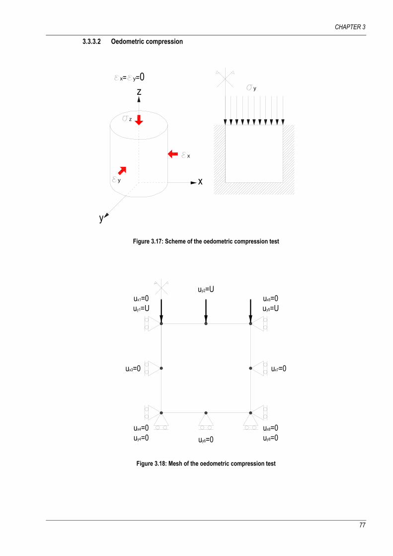
CHAPTER 3
77
3.3.3.2 Oedometric compression
x
y
z
x
y
z
x= y=0y
Figure 3.17: Scheme of the oedometric compression test
ux1=0uy1=U
uy2=U
ux3=0
ux5=0uy5=U
ux4=0uy4=0
ux8=0uy8=0uy6=0
ux7=0
Figure 3.18: Mesh of the oedometric compression test

FEM MODEL
78
3.3.3.3 Triaxial compression
x
y
z
x
y
z
x= y=constant
x
y
x=constantz increases y increases
Figure 3.19: Scheme of the triaxial compression test
ux1=0uy1=Uy
uy2=Uy
ux3=0
ux5=Ux
uy5=Uy
ux7=Ux
ux4=0uy4=0
ux8=Ux
uy8=0uy6=0
Figure 3.20: Mesh of the triaxial compression test

CHAPTER 3
79
N d.o.f. d.o.f. N. condition Value u.o.m.
1 pg 1 Impose pg Pa
2 Impose air flux sm
kg2
2 pc 1 Impose pc Pa
2 Impose vapour flux sm
kg2
3 Impose value of RH %
4 Impose vapour pressure Pa
3 T 1 Impose T K
2 Impose heat flux Km
W2
3 Impose room T (convective) K
4 Impose room T (radiation) K
4 ux 1 Impose ux m
2 Impose sx Pa
5 uy 1 Impose uy m
2 Impose sy Pa
Table 3.2: Model conditions
3.3.4 Remarks on the F.E.M. modelling approach
As mentioned before, one single eight node square element of 1 m has been usually adopted to simulate the isotropic,
oedometric and triaxial tests of the validation phase of this work.
The dimension of this element was chosen for simplicity so that the axial strain equals the axial displacement (in small
strain).
Moreover, during the computations, gravity acceleration was neglected. This was motivated from the experimental
behaviour of the samples during the common geotechnical laboratory tests, in which the effect of the gravity load on the
stress field can be neglected due to the small dimension of the samples (i.e. 72×19 mm, Figure 3.21) and the applied
confining pressure. In addition, also the model drivers neglect the gravity load.
The quadratic element was preferred to the linear one because it is the typical finite element used to discretize the 2D
displacement field of saturated and unsaturated porous media.
Accuracy of the numerical solution was analyzed by solving the same isotropic compression test (see 4.4.3 Elastoplastic
isotropic compression in isothermal condition) with 1 quadratic element of the dimension of a geotechnical sample
(Figure 3.21 integrated with 3×3 gauss points), 30 quadratic element (Figure 3.22), 1 quadratic element of unit

FEM MODEL
80
dimension (Figure 3.23 and Figure 3.24 integrated with 2×2 or 3×3 gauss points respectively), 100 quadratic element
(Figure 3.25) and also discretizing the unit domain with 1 quadratic four node element (Figure 3.26 integrated with 2×2
gauss points).
Figure 3.27 and Figure 3.28 show the numerical results, where it can be observed that the solution obtained with 1 unit
element is accurate from the numerical point of view. Instead the Figure 3.29 shows that the numerical solution obtained
with the use of 1 four node element is also accurate.
As a further remark it is observed that in case of strain localization test, a suitable spatial discretization has to be used in
[San06]. 72
Ø38
19 72
19
N° OF ELEMENTS1
HEIGHT72 mm
WIDTH19 mm
ORDER OFINTEGRATION
3×3
Figure 3.21: Eight node quadrilateral element used
72
Ø38
19 72
19
N° OF ELEMENTS30
HEIGHT72 mm
WIDTH19 mm
ORDER OFINTEGRATION
3×3
Figure 3.22: Eight node quadrilateral elements used

CHAPTER 3
81
N° OF ELEMENTS1
HEIGHT1 m
WIDTH1 m
ORDER OFINTEGRATION
2×2
1 m
1 m
Figure 3.23: Eight node quadrilateral element used
N° OF ELEMENTS1
HEIGHT1 m
WIDTH1 m
ORDER OFINTEGRATION
3×3
1 m
1 m
Figure 3.24: Eight node quadrilateral element used
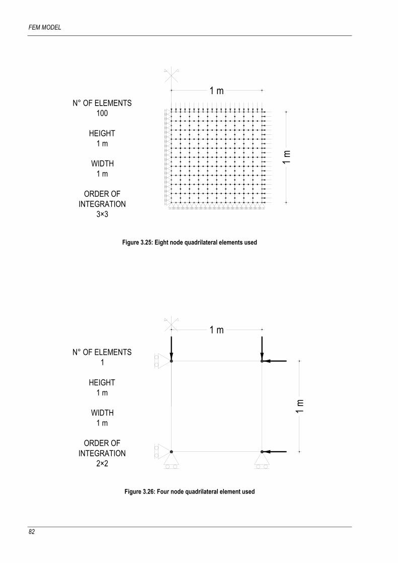
FEM MODEL
82
N° OF ELEMENTS100
HEIGHT1 m
WIDTH1 m
ORDER OFINTEGRATION
3×3
1 m
1 m
Figure 3.25: Eight node quadrilateral elements used
N° OF ELEMENTS1
HEIGHT1 m
WIDTH1 m
ORDER OFINTEGRATION
2×2
1 m
1 m
Figure 3.26: Four node quadrilateral element used

CHAPTER 3
83
-0,15
-0,13
-0,11
-0,09
-0,07
-0,05
-0,03
-0,01
1 10 100 1000
Mean stress [kPa]
Volu
met
ric
stra
in [-]
1x1 - 1 element - 3×3
Sample 1 element
Sample 30 elements
Figure 3.27: Comparison with different meshes and sample dimensions
-0,15
-0,13
-0,11
-0,09
-0,07
-0,05
-0,03
-0,01
1 10 100 1000
Mean stress [kPa]
Volu
met
ric
stra
in [-]
1x1 - 1 element - 3×3
1x1 - 1 element - 2×2
1x1 - 100 element - 3×3
Figure 3.28: Comparison with the same sample dimensions and different discretizations

FEM MODEL
84
-0,15
-0,13
-0,11
-0,09
-0,07
-0,05
-0,03
-0,01
1 10 100 1000
Mean stress [kPa]
Volu
met
ric
stra
in [-]
1x1 - 1 element - 3×3 - 8 nodes
1x1 - 1 element - 2×2 - 4 nodes
Figure 3.29: Comparison with the same sample dimensions and different elements

CHAPTER 3
85
References
[Bia03] Bianco, M., Bilardi, G., Pesavento, F., Pucci, G., Schrefler, B.A.: A frontal solver tuned for fully coupled
non-linear hygro-thermo-mechanical problems. Int. J. Numer. Meth. Engng. 57, 1801-1818 (2003).
[Cou1776] Coulomb, C. A. (1776) Essai sur une application des règles des maximis et minimis a quelques problèmes
de statique relatifs a l'architecture. Mem. Acad. Ro. Pres. Divers Sav. 5, 7.
[Dru59] Drucker, D. C. (1959) A definition of stable inelastic material. Trans. ASME. 26, 00-00.
[G&S96] D.Gawin, B.A.Schrefler, ‘Thermo-hydro-mechanical analysis of partially saturated porous materials’,
Engng.Comp., 13(7), 113-143 (1996).
[Gaw96] D.Gawin, P.Baggio, B.A.Schrefler, ‘Modelling heat and moisture transfer in deformable porous building
materials’, Arch. of Civil Engng. 42(3), 325-349, (1996).
[Hum76] Humpheson. C. (1976) Finite element analysis of elasto-vIsco-plastic soils. PhD thesis. University College
of Swansea.
[L&S98] Lewis R.W. and Schrefler B.A. The Finite Element Method in the Static and Dynamic Deformation and
Consolidation of Porous Media. J. Wiley, Chichester 1998.
[M&Z84] Mroz. Z. and Zienkiewicz. O. C. (1984) Uniform formulation of constitutive equations for clays and sands.
Mechanics of Engineering Materials. C. S. Desai and R. H. Gallagher (eds). Wiley, Chichester. Ch. 22, pp.
415-449.
[N&Z72] Nayak. G. C. and Zienkiewicz. O. C. (1972) Convenient form of stress invariants for plaslicity. Proc. ASCE.
98 (ST4). 949-53.
[Nay75] Naylor, D. J. (1975) Non-linear finite element models for soils. PhD thesis. University College of Swansea.
[Nor80] Norris, V. A. (1980) The elasto-plastic analysis of soil consolidation with special reference to kinematic
hardening. PhD thesis, University College of Swansea.
[R&B68] Roscoe. K. H. and Burland, J. B. (1968) On the generalised stress-strain behaviour of 'wet' clay, in
Engineering Plasticity. Heyman, J.. Lechie, F. A. Cambridge University Press. Cambridge. pp. 535-609.
[R&P63] Roscoe. K. H. and Poorooshasb, H. B. (1963) A theoretIcal and experimental study of strains in triaxial
compression tests on normally consolidated clays. Géotechnique. 13(1). 12-34.
[R&S63] Roscoe. K. H. Schofield. A. N. and Thurairajah, A. (1963) Yielding of clays in states welter than critical.
Géotechnique. 13(3), 211-IO.
[S&G96] B.A.Schrefler, D.Gawin, The effective stress principle: incremental or finite form? Int. J. for Num. and Anal.
Meth. in Geomechanics, 20(11), 785-815, (1996).
[S&W68] Schofield. A. N. and Wroth. C. P. (1968) Critical State Soil Mechanics. McGraw-Hill, New York.
[San05] L. Sanavia, F. Pesavento, B.A. Schrefler, Finite element analysis of non-isothermal multiphase
geomaterials with application to strain localization simulation, Computational Mechanics Vol. 466, (2005)
(DOI 10.1007/s00466 -005-0673-6).
[San06] Sanavia L., F. Pesavento, B.A. Schrefler (2006) Finite element analysis of non-isothermal multiphase
geomaterials with application to strain localisation simulation, Computational Mechanics, 37 (4), 331-348.

FEM MODEL
86
[Z&M84] Zienkiewicz. O. C. and Mroz. Z. (1984) Generalized plasticity formulation and applications to
geomechanics. Mechanics of Engineering Materials. C. S. Desai and R. H. Gallagher (eds). Wiley,
Chichester. Ch. 33, pp. 655-679.
[Z&T89] Zienkiewicz O. C., Taylor R. L., The Finite Element Method, Vol. 1, 4th ed., Mc Graw Hill, London (1989).
[Z&T91] Zienkiewicz O. C., Taylor R. L., The Finite Element Method, Vol. 2, 4th ed., Mc Graw Hill, London (1991).
[Zie75] Zienkiewicz, O. C. Humpheson, C. and Lewis, R. W. (1975) Associated and non-associated viscoplasticity
and plasticity in soil mechanics. Géotechnique, 25(4), 67 1 -89.
[Zie77] Zienkiewicz. O. C. (1977) The Finite Element Method. McGraw-Hill. London.

CHAPTER 4
87
4 THE THERMO-ELASTO-PLASTIC CONSTITUTIVE MODEL
ACMEG-T
4.1 TEMPERATURE EFFECTS IN SOILS
4.1.1 Thermal problem in soils
Thermal effects in geomechanical problems are important for several specific applications as, for instance, nuclear
waste isolation and the use of soil deposits for heat energy storage. Some other applications are related to geothermal
structures, petroleum drilling, injection and production activity, zones around buried high-voltage cables and in soil tests
for to take into account the thermal problem during the time from the situ to the laboratory. In more of the applications
mentioned above, the temperature values considered are between 5 and 95 °C, but, in case of failure situation for
nuclear waste storage, the temperature can reach 400 °C. Research work has shown that an increase in temperature
affects soil characteristics (friction angle, permeability, elastic modulus, etc.) and behaviour is different for the influence
of soil type or stress state or drainage condition or more.
The effect of the temperature, and in greater way the effect of the high temperature, on soils behaviour is not completely
clear, although the relevance of the thermo-mechanical applications and the many test in the literature. This is due to the
complex influence of temperature on the behaviour of soils, and the fact that thermo-mechanical testing of soils is much
more complex than conventional isothermal testing. In fact, for the presence of temperature is necessary an additional
reliable system with specific property. System must maintains constant temperature on sample, must have an heating
equipment that work independently from the other part and more.
In this chapter, for the ACMEG-T model, the soils that we want to model are clay. The model has been developed by the
research group of the Professor Lyesse Laloui in Lausanne at the EPFL, Ecole Polytechnique Federale de Lausanne,
[M&L97] and [L&C08], and it represents an extension in non-isothermal conditions of the modified CAM-CLAY model.
4.1.2 Thermo-mechanical behaviour of soils
Clay is a material with a not common behaviour under non isothermal conditions. In fact, in normally consolidated
conditions (NC), clay contracts under heating, and this is atypical of the normal material, while in over consolidated
conditions, clay dilate under heating (see Figure 4.2). Another important aspect of clay under heating is that a not
negligible part of this contractive deformation is irreversible. Moreover, from the experimental tests, it is possible to note
that the variation of volume is non-linear during heating and linear upon cooling.
The irreversibility of strain due to thermal loading is an evident thermal hardening.
It is clearly impossible to simulate this behaviour with a thermo-elastic model cause the irreversibility of strain, it is
necessary a more complex model, a thermo-elastoplastic model.

THE THERMO-ELASTO-PLASTIC CONSTITUTIVE MODEL ACMEG-T
88
Plasticity induced by temperature, is due to and explained by a combination of certain mechanisms at micro level. The
first one is the partial collapse of the soil structure and a decrease in void ratio until a number of additional bonds are
formed, these bonds are able to allow the soil to carry the stress at the higher temperature [C&M68]. The second micro-
mechanical processes is the thermal degradation of the adsorbed layer, which tends to group particles closer together
and may produce large voids between the platelet aggregates [Pus87]. Another mechanism is the difference in rigidity
and in thermal expansion between the dissimilar minerals forming the solid skeleton that generates a modification of the
contact force networks as temperature increases [Kin76]. The last mechanism of soil under temperature increase, if the
particle arrangement are assumed to be fixed, is the increase of pore size and the inter-particle distance due to the
thermal expansion of each soil constituent that would produce a global dilation of the solid skeleton. This change the
equilibrium between the Van der Waals attractive forces and the electrostatic repulsive forces, which results in the
particles rearranging to reach a new equilibrium [Lal01].
A good indicator of the importance of the water-mineral interactions in clays is the soil plasticity index, Demarks and
Charles [D&C82] show this axpect for six different clays at normally consolidated state. The volumetric thermo-plastic
strain of normally consolidated soil, reported by unit temperature change, seems to increase when the plasticity index
increases (Figure 4.1).
Figure 4.1: Relation between the plasticity index and the temperature-induced contractile strain (redrawn from [Fra08]).

CHAPTER 4
89
Table 4.1: Contractile volumetric strain induced by a temperature change at constant mean effective stress in different NC
clay. Correlation with the plasticity index of the soil. Thermal cycle: Yes: Heating-cooling cycle; No: only heating. (Redrawn
from [Fra08]).
Different by the behaviour of NC clays under temperature increase are OC clays. Indeed, the latter show an almost
completely reversible deformation after a thermal cycle of heating and cooling. The micro-mechanical processes that
could explain the thermoplasticity of NC soils remain active for highly OC soils but, the low stress level does not supply
enough acting force between particles to modify the soil structure. In that sense, the particle arrangement remains fixed,
and only thermo-elastic strain is produced.
In conclusion the typical behaviour of NC clays under a thermal cycle of heating and cooling is the production of
irreversible deformations of contraction and the behaviour of OC clays is, at the opposite, the reversibility of the
deformations of dilatation (Figure 4.2).

THE THERMO-ELASTO-PLASTIC CONSTITUTIVE MODEL ACMEG-T
90
Figure 4.2: Typical volumetric strain induced by heating-cooling cycles at different overconsolidation ratios. (a) Boom clay
[Bal91]; (b) Bangkok clay [A-N07]; (c) Kaolin clay [C&L04]; (d) Pasquasia clay [DeO96]. (Redrawn from [Fra08]).

CHAPTER 4
91
4.1.3 Temperature effect on preconsolidation pressure
In this work, is indicate with p’c the preconsolidation pressure, that is the stress yield limit that separates the elastic part
from the plastic one in terms of behaviour under isotropic or oedometric conditions. Several results from the literature
show a decrease in the preconsolidation pressure with increasing temperature. Laloui and Cekerevac [L&C03] proposed
the following equation to describe this thermo-mechanical behaviour:
−=
0
'0
' log1TT
pp Tcc γ [4.1]
where p’c is the preconsolidation pressure at a given temperature T
p’c0 is the preconsolidation pressure at the reference temperature T0
gT is a material parameters
Others author proposed the following different relations:
( )[ ]0'0
' TTcc epp −−= α
Cui et al., 2000 [4.2]
( ) ( )[ ]00201'0
' 2 TTTTaTTapp cc −−+−+= Hueckel and Baldi, 1990 [4.3]
( )[ ]0'0
' 1 TTCpp cc −+= Boudali et al., 1994 [4.4]
n
cc TT
pp
=
0
'0
' Moritz, 1995 [4.5]
Figure 4.3: Relation between Ip and ggggT (redrawn from [Fra08]).

THE THERMO-ELASTO-PLASTIC CONSTITUTIVE MODEL ACMEG-T
92
Table 4.2: Ip, ggggT and reduction of p’c0 from T0 and T1 (redrawn from [Fra08]).
4.1.4 Temperature effects on shearing behaviour
In terms of elastic behaviour of soil, experimental results show what the temperature has a stiffening effect. Cekerevac
and Laloui [C&L04] observed an higher soil stiffness in Kaolin clay (Figure 4.4 a) as for Kuntiwattanakul et al. [Kun95] in
MC clay where, the increase of the secant modulus is confirmed both for NC clay and OC clay (Figure 4.4 b).
Approximately the same results were found from Abuel-Naga [A-N05] in Bangkok clay.
Figure 4.4: Secant elastic modulus at different temperature for a) Kaolin clay [C&L04] and b) MC clay [Kun95]. (Redrawn
from [Fra08])
Burghignoli et al. [Bur00] instead found that in Tody clay there is not a significant effect of temperature on stiffness of
material if the temperature is the highest temperature experienced by the soil. However, they noted that a thermal cycle
performed before triaxial shearing tends to increase the stiffness of the soil.

CHAPTER 4
93
Not unique is the behaviour of soil under the increase of temperature in terms of shear strength, some research in fact
had found a decrease in strength with heating and others, contrariwise, had found slightly increase of strength.
A series of experimental results summarised by Cekerevac and Laloui [C&L04] tend to confirm that the friction angle at
the critical state can either slightly increase or decrease with temperature. However, comparison is not always possible
due to the variability in experimental techniques, stress and strain paths and drainage conditions during heating and
shearing. For instance, Hueckel and Pellegrini [H&P89] observed that the slope of the friction angle at the critical state of
Pontida clay is unaffected by temperature under both drained and undrained shearing. In contrast, the same authors
noticed a slight increase in friction angle of Boom clay under undrained shearing.
In term of maximal deviatoric stress, Cekerevac [Cek03] in tests performed in a Kaolin clay and Kuntiwattanakul et al.
[Kun95] in tests performed MC clay observed a slight increase in the peak strength during heating (Figure 4.5).
Because of the different results found in literature it is not possible to draw any general conclusion. In fact, for instance,
Abuel-Naga et al. [A-N06] also noticed an increase of the maximal deviatoric stress upon triaxial shearing of normally
consolidated Bangkok clay, while Hueckel et al. [Hue98] suggested that the peak strength of a Spanish clay decreases
by about 25% for a temperature increase from 22° to 120 °C.
Figure 4.5: Maximal deviatoric stress at different temperature for a) Kaolin clay [Cek03] and b) MC clay [Kun95]. (Redrawn
from [Fra08])
4.2 ACMEG-T MODEL
4.2.1 Introduction
The ACMEG-T model [Lal05] [L&F08] is the extension to non-isothermal conditions of the model ACMEG [M&L97] and
[L&C08]. The model can reproduce the different behaviour of NC and OC clay, the decrease of preconsolidation
pressure, and if present, the variation of frictional angle value with temperature.
Here, the considered temperature range is from 5 °C to 95 °C.
THE THERMO-ELASTO-PLASTIC CONSTITUTIVE MODEL ACMEG-T
94
4.2.2 ACMEG Model
The ACMEG model ([M&L97] and [L&C08]) (Advanced Constitutive Model for Environmental Geomechanics), here
presented as in [Fra08], is composed of two parts, one that take into account the volumetric response upon isotropic
compression, and one that take into account the stress-strain behaviour upon soil distortions (deviatoric loading).
The model considers under isotropic conditions:
1. the effect of stress level on the elastic rigidity of soil;
2. the plastic volumetric strain generated when the preconsolidation pressure is surpassed;
3. the progressive transition between the reversible elastic and the irreversible elasto-plastic response;
4. the existence of an elastic nucleus in the stress space in which the produced strains are fully reversible;
5. the volumetric response of soil upon several isotropic loading-unloading-reloading cycles (without
accommodations effects).
The model considers under deviatoric conditions:
1. the effect of stress level on the elastic rigidity of soil;
2. the unique critical state reached upon various distortional paths;
3. the hardening process occurring from the elastic domain to the critical state of normally or slightly
overconsolidated soils;
4. the peak behaviour observed on distortion paths of highly overconsolidated soils;
5. the progressive transition between the reversible responses and the full mobilization of the hardening or
softening processes;
6. the existence of an elastic nucleus in the stress space in which the produced strains are fully reversible;
7. the accurate volumetric response upon distortional paths which can involve a non-associated flow rule.
4.2.2.1 Non linear elasticity
The elastic moduli present a strong dependency from the mean effective stress and the equations governing this
phenomenon are:
en
refref p
pK=K
′′
[4.6]
for the bulk modulus, and:
en
refref p
pG=G
′′
[4.7]
for the shear modulus
where Kref is the bulk modulus at the reference mean effective stress p’ref
Gref is the shear modulus at the reference mean effective stress p’ref
ne is a material parameter
It is possible prove that this non-linear elasticity relation is non-conservative in terms of the work input. Indeed, upon any
purely elastic loading-unloading path for which the final stress state corresponds to the initial one, the total work input

CHAPTER 4
95
must be null. The use of the proposed elastic module does not guarantee such a conservation condition. In other words
the elastic behaviour of model is ipoelastic.
4.2.2.2 The multi-mechanism theory
Starting from the Original Cam-Clay model and its deviatoric yielding mechanism, adding an isotropic mechanism in
agreement with Hujeux [Huj79], it is possible to build a two-mechanism model.
The isotropic mechanism have the following form:
0=′−′= ciso ppf [4.8]
where p’c is the preconsolidation pressure and evolves according to the equation
( )pvepp cc
βε0′=′ [4.9]
where b is the plastic compressibility modulus
The two yield functions define a closed domain in the effective stress space inside which the behaviour of the material is
reversible. If the volumetric plastic strain increases due to the activation of one of the mechanisms, the yield limit of the
other mechanism will also move. When the two mechanisms are activated simultaneously, two consistency conditions
must be met leading to two interrelated plastic multipliers ( lpiso and lp
dev). Thus, the total increment of volumetric
plastic strain is:
devp
visop
vpv ddd ,, εεε += [4.10]
where isopvd ,ε is the volumetric plastic strain induced by the isotropic mechanism
devpvd ,ε is the volumetric plastic strain induced by the deviatoric mechanism
4.2.2.3 Improvement of deviatoric mechanism of Cam Clay model
Ratio between the preconsolidation pressure and the critical pressure is equal to 2.718 in the Original Cam Clay model.
In the ACMEG model, this ratio it is not constant, but, as in realty, depends from the material and it is indicate with d
[Huj79]. The deviatoric yield limit begins now:
0ln1 =
′′⋅−′−=
cdev p
pdpMqf [4.11]
where
cr
c
pp
d′′
= [4.12]
and where p’cr is the critical pressure.
Moreover, for simulate better the heavily overconsolidated soils, the Cam Clay model is modified by introducing the
parameter b for the control of the shape of the yield limit. The deviatoric yield limit begins as:
0ln1 =
′′⋅⋅−′−=
cdev p
pdbpMqf [4.13]

THE THERMO-ELASTO-PLASTIC CONSTITUTIVE MODEL ACMEG-T
96
This expression is similar to the failure locus proposed by Nova and Wood [N&W79] with M
b*β= , where *β is a
parameter of the Nova-Wood model. The b parameter varies from 0 (corresponding to a Mohr-Coulomb criterion) to 1
(for the Original Cam-Clay model) as shown in Figure 4.6. As stated by Hujeux [Huj85], the role of this parameter is
particularly important for highly overconsolidated soils. Generally, the value of b is lower for sand than for clays.
Figure 4.6: Deviatoric yield limit for different values of b (redrawn from [Fra08])
4.2.2.4 Degree of mobilization of the isotropic mechanism
Typical isotropic compression experimental results on a remoulded soil, as shown in Figure 4.7, clearly exhibit
progressive mobilization of the plasticity before reaching the virgin consolidation line.
Figure 4.7:Comparison between experimental results [Jam03] and a numerical simulation (redrawn from [Fra08])

CHAPTER 4
97
Therefore, even before surpassing the isotropic yield limit (i.e. the preconsolidation pressure), the soil undergoes
generally irreversible strains upon isotropic loading. This behavioural feature can have a major effect on the response of
an overconsolidated soils submitted to loading-unloading cycles. In order to reproduce this effect, the model needs to be
improved by means of an additional constitutive artifice. The isotropic yield limit is modified as follows [Huj79]:
0=⋅′−′= isociso rppf [4.14]
where riso is the degree of mobilization of the isotropic mechanism.
During loading, riso is a hyperbolic function of the volumetric plastic strain induced by the isotropic mechanism (Figure
4.8), isopv
,ε :
isopv
isopve
isoiso crr ,
,
ε
ε
++= [4.15]
and (see [Huj85] and [Fra08])
( ) isopv
isoiso d
cr
dr ,21ε
−= [4.16]
where c is a material parameter
eisor is the radius of the isotropic elastic nuclei inside which the produced strains are fully reversible.
During unloading the behaviour is purely elastic.
Figure 4.8: dependence of riso by volumetric plastic strain
In the same way as the isotropic mechanism, the deviatoric mechanism needs to be enhanced by a progressive
plasticity process inside the external deviatoric yield limit. Hujeux [Huj79] proposed to introduce an additional hardening
variable, the deviatoric plastic strain pdε , governing the evolution of the degree of mobilization of the deviatoric
mechanism rdev. The deviatoric yield limit is modified as follows:
0ln1 =⋅
′′⋅⋅−′−= dev
cdev r
ppd
bpMqf [4.17]
During loading, rdev is an hyperbolic function of the deviatoric plastic strain pdε :

THE THERMO-ELASTO-PLASTIC CONSTITUTIVE MODEL ACMEG-T
98
pd
pde
devdev arr
ε
ε
++= [4.18]
and (see [Huj85] and [Fra08])
( ) pd
devdev d
ar
dr ε21−= [4.19]
where a is a material parameter
edevr is the radius of the deviatoric elastic nuclei inside which the produced strains are fully reversible.
4.2.2.5 Isotropic plastic mechanism
Here, the constitutive equations are summarized in a concise way. Within the small strain assumptions, the total strain
increment vector can be written as follow:
pij
eijij ddd εεε += [4.20]
and, the total strain increment induced by plasticity (hardening of the material) is a linear combination of two irreversible
processes: an isotropic as well as a deviatoric process. Therefore, the “total” plastic strain increment, pijdε , is the sum
of “partial” plastic strain increments, induced by the isotropic and the deviatoric mechanisms, isopijd ,ε and devp
ijd ,ε ,
respectively:
devpij
isopij
pij ddd ,, εεε += [4.21]
The isotropic yield limit fiso is:
0=⋅′−′= isociso rppf [4.22]
where ( )pvepp cc
βε0′=′
isopv
isopve
isoiso crr ,
,
ε
ε
++=
The flow rule is assumed to associated (fiso=giso) and hence:
3,
piso
ii
isopiso
isopii
gd
λ
σλε =
′∂∂= [4.23]
The plastic multiplier, pisoλ , is determined using Prager’s consistency equation [Pra49].
4.2.2.6 Deviatoric plastic mechanism
The deviatoric yield limit fdev is:
0ln1 =⋅
′′⋅⋅−′−= dev
cdev r
ppd
bpMqf [4.24]
where Φ
ΦM=
′−′
sin3sin6
is the slope of the critical state line (CSL) in the p’-q plane,
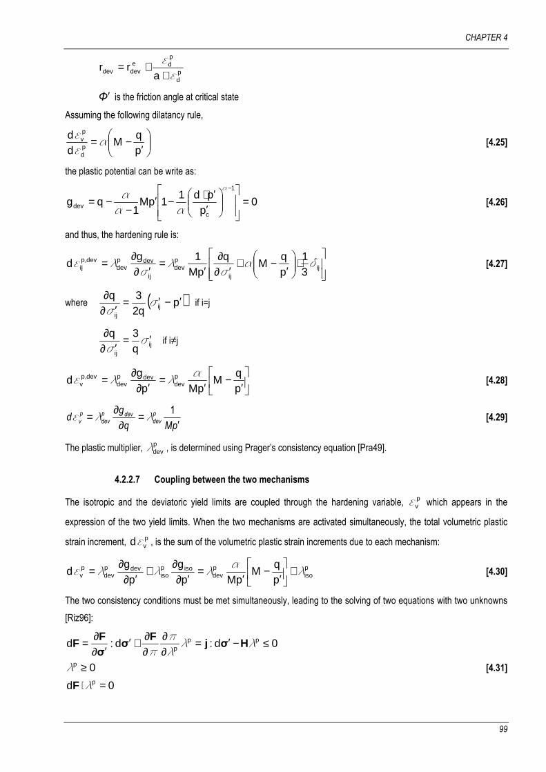
CHAPTER 4
99
pd
pde
devdev arr
ε
ε
++=
Φ′ is the friction angle at critical state
Assuming the following dilatancy rule,
′−=
pq
Mdd
pd
pv αε
ε [4.25]
the plastic potential can be write as:
01
11
1
=
′′⋅−′
−−=
−α
αα
α
cdev p
pdpMqg [4.26]
and thus, the hardening rule is:
⋅
′−+
′∂∂
′=
′∂∂= ij
ij
pdev
ij
devpdev
devpij p
qM
qpM
gd δα
σλ
σλε
311,
[4.27]
where ( )pq
qij
ij
′−′=′∂
∂σ
σ 23
if i=j
ijij q
qσ
σ′=
′∂∂ 3
if i≠j
′−
′=
′∂∂=
pq
MpMp
gd p
devdevp
devdevp
v
αλλε ,
[4.28]
pMq
gd p
devdevp
devpv ′
=∂
∂= 1λλε [4.29]
The plastic multiplier, pdevλ , is determined using Prager’s consistency equation [Pra49].
4.2.2.7 Coupling between the two mechanisms
The isotropic and the deviatoric yield limits are coupled through the hardening variable, pvε which appears in the
expression of the two yield limits. When the two mechanisms are activated simultaneously, the total volumetric plastic
strain increment, pvdε , is the sum of the volumetric plastic strain increments due to each mechanism:
piso
pdev
isopiso
devpdev
pv p
qM
pMpg
pg
d λα
λλλε +
′−
′=
′∂∂+
′∂∂= [4.30]
The two consistency conditions must be met simultaneously, leading to the solving of two equations with two unknowns
[Riz96]:
0
0
0::
=⋅≥
≤−′=∂∂
∂∂+′
′∂∂=
p
p
ppp
d
ddd
λ
λ
λλλ
π
π
F
HσjF
σσ
FF
[4.31]
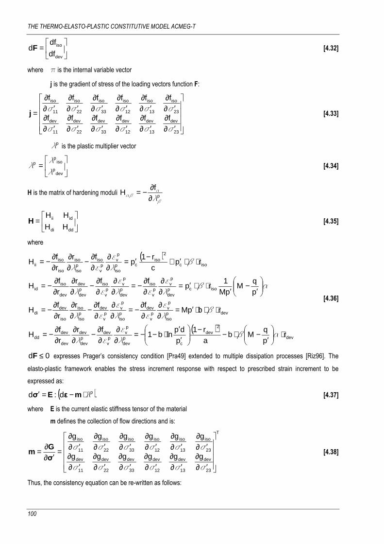
THE THERMO-ELASTO-PLASTIC CONSTITUTIVE MODEL ACMEG-T
100
=
dev
iso
df
dfdF [4.32]
where p is the internal variable vector
j is the gradient of stress of the loading vectors function F:
′∂∂
′∂∂
′∂∂
′∂∂
′∂∂
′∂∂
′∂∂
′∂∂
′∂∂
′∂∂
′∂∂
′∂∂
=
231312332211
231312332211
σσσσσσ
σσσσσσ
devdevdevdevdevdev
isoisoisoisoisoiso
ffffff
ffffff
j [4.33]
pλ is the plastic multiplier vector
=
devp
isop
p
λ
λλ [4.34]
H is the matrix of hardening moduli p
fH
β
ααβ λ∂
∂−=
=
dddi
idii
HH
HHH [4.35]
where
( )
( )dev
dev
cpdev
pv
pv
devpdev
dev
dev
devdd
devpiso
pv
pv
devpiso
pv
pv
devpiso
iso
iso
devdi
isocpdev
pv
pv
isopdev
pv
pv
isopdev
dev
dev
isoid
isociso
cpiso
pv
pv
isopiso
iso
iso
isoii
rpq
Mbar
pdp
bfr
rf
H
rbpMffr
rf
H
pq
MpM
rpffr
rf
H
rpcr
pfr
rf
H
⋅
′−⋅−−
′′
⋅−−=∂∂
∂∂−
∂∂
∂∂−=
⋅⋅⋅′=∂∂
∂∂−=
∂∂
∂∂−
∂∂
∂∂−=
′−
′⋅⋅′=
∂∂
∂∂−=
∂∂
∂∂−
∂∂
∂∂−=
⋅⋅′+−′=∂∂
∂∂−
∂∂
∂∂−=
αβλ
ε
ελ
βλ
ε
ελ
ε
ελ
αβλ
ε
ελ
ε
ελ
βλ
ε
ελ
2
2
1ln1
1
1
[4.36]
0≤Fd expresses Prager’s consistency condition [Pra49] extended to multiple dissipation processes [Riz96]. The
elasto-plastic framework enables the stress increment response with respect to prescribed strain increment to be
expressed as:
( )pdd λ⋅−=′ mεEσ : [4.37]
where E is the current elastic stiffness tensor of the material
m defines the collection of flow directions and is:
T
devdevdevdevdevdev
isoisoisoisoisoiso
gggggg
gggggg
′∂∂
′∂∂
′∂∂
′∂∂
′∂∂
′∂∂
′∂∂
′∂∂
′∂∂
′∂∂
′∂∂
′∂∂
=′∂
∂=
231312332211
231312332211
σσσσσσ
σσσσσσ
σ
Gm [4.38]
Thus, the consistency equation can be re-written as follows:

CHAPTER 4
101
( )
0
0
0::::
=⋅≥
≤⋅+−=
p
p
p
d
dd
λ
λ
λ
F
mEjHεEjF
[4.39]
4.3 ACMEG-T MODEL
In this sections, the ACMEG model is modiefied, taken into account the temperature influence on the behaviour of soils,
to obtain the ACMEG-T model.
4.3.1 Thermo elasticity
The non-isothermal case causes, in elasticity, a reversible strain increment:
dTdEddd ijTklijklTeij
meij
eij ,
1 βσεεε −′=+= − [4.40]
where ijT ,β is the thermal expansion tensor which depends on the temperature, T.
Considering isotropic thermal behaviour, one can express ijT ,β as ijsijT δββ ′=31
, with sβ ′ being the volumetric
thermal expansion coefficient of the solid skeleton.
The volumetric and deviatoric parts of the tensor of the elastic strain increment are, respectively:
dTKpd
ddd sTev
mev
ev βεεε ′−
′=+= [4.41]
Gdq
ddd Tev
mev
ed 3
=+= εεε [4.42]
The volumetric thermal expansion coefficient of the solid skeleton, sβ ′ , it is not constant but increases with temperature
and decreases as stress level increases [L&C03]:
( )[ ]ξζββ 00 TTss −+′=′ [4.43]
where 0sβ ′ is the isotropic thermal expansion coefficient at a reference temperature, T0 (usually ambient
temperature)
Tn
cr
pp
′′
= 0ξ is the ratio between the initial critical state pressure at ambient temperature, p’cr0, and the
mean effective stress, p′ and nT is a material parameter,
ζ is the slope of the variation of sβ ′ with respect to the current temperature, T and when 1=ξ
ζ could be approximated as proposed by Laloui [Lal93] with the following reletionship:
C 1000
°′
−= sβζ [4.44]
and its dimension is °C-2.

THE THERMO-ELASTO-PLASTIC CONSTITUTIVE MODEL ACMEG-T
102
Obviously, the relation [4.43] with the approximation C 100
0
°′
−= sβζ [4.44][4.44], is correct only for temperature
between 20 °C (room temperature) and 95 °C, as mentioned. In fact, when T-T0 is greater then 100 °C, the coefficient
sβ ′ begins negative.
4.3.2 Thermo plasticity
The thermo-plastic strain increment can be expressed as the part of the total strain increment which is not recoverable:
klijklijTijeijij
pij dEdTdddd σβεεεε ′−+=−= −1
, [4.45]
The yield limits of the isotropic and deviatoric mechanism, respectively, are recalled and the temperature-induced
modifications of those relations are presented.
4.3.2.1 Isotropic thermo-plastic mechanism
The thermal effect on the isotropic mechanism is introduced through the evolution of the preconsolidation pressure p’c0
with temperature (Figure 4.9).
Figure 4.9: a) Isotropic yield limit. b) dependency of p’c from ggggT [L&C03] (redrawn from [Fra08])
As shown in section 4.1.3, several authors suggested analytical expressions to describe the shrinkage of the yield limit
with increasing temperature. The evolution of p’c with temperature being rapid for low temperature changes and
becoming asymptotic for the high ones, the logarithmic function of Laloui and Cekerevac [L&C03] is a very suitable
expression to model this phenomenon. The thermo-mechanical evolution of isotropic yield surface is expressed as:
( ) 0log10
0 =
−′−′= isoTciso r
TT
eppfpv γβε
[4.46]
where p’c is the preconsolidation pressure at a given temperature T
p’c0 is the preconsolidation pressure at the reference temperature T0
gT is a material parameters

CHAPTER 4
103
b is the plastic compressibility modulus
pvε is the volumetric plastic strain
riso is the degree of plastification of the isotropic mechanism
The flow rule of the isotropic mechanism remains unchanged regarding to the isothermal mechanism [4.23].
4.3.2.2 Deviatoric thermo-plastic mechanism
Starting from the equation seen in section 4.2.2.6 [Huj79]
0ln1 =⋅
′′⋅⋅−′−= dev
cdev r
ppd
bpMqf [4.47]
where p’c is the preconsolidation pressure
d is the ratio between the preconsolidation pressure, p’c, and the critical pressure, p’cr
b is a material parameter defining the shape of the deviatoric yield limit
rdev is the degree of plastification of the deviatoric mechanism
M is the slope of the critical state line in the p’−q plane
As shown by Laloui [Lal03], the friction angle may be depend on temperature with the following expression:
( )00 TTgMM −−= [4.48]
where M0 is the is the slope of the critical state line at ambient temperature T0
g is an average slope of variation of friction angle at critical state with temperature
Obviously, if for some soil there is no influence of temperature on the frictional angle, the parameter g is equal to zero.
Figure 4.10: Effective stress path on Boom clay in isotropic condition. Influence of temperature on M (redrawn from [Fra08])
Thus, the deviatoric yield surface becomes, under non-isothermal conditions:
( )[ ] 0
log1
ln1
00
00 =⋅
−′
′⋅⋅−′−−−= dev
Tc
dev r
TT
ep
pdbpTTgMqf
pv γβε
[4.49]
The flow rule of the deviatoric mechanism remains unchanged regarding to the isothermal mechanism [4.25] and [4.29].

THE THERMO-ELASTO-PLASTIC CONSTITUTIVE MODEL ACMEG-T
104
4.3.2.3 Coupling between the two thermo-plastic mechanisms
The coupling between the two thermo-plastic mechanisms is similar to the isothermal model. However, inclusion of the
derivation of the yield limits with respect to temperature is required in the consistency conditions for multi-mechanism
due to the evolution of both yield limits with temperature state [Pra58]. In that sense, the effective stress and the
temperature are the two state variables of the model:
0
0
0::
=⋅≥
≤⋅−⋅+′=⋅∂∂⋅
∂∂+⋅
∂∂+′
′∂∂=
p
p
ppp
d
dTddTT
dd
λ
λ
λλλ
π
π
F
HtσjFF
σσ
FF
[4.50]
where t is the temperature-gradient of the loading function F
The stress increment is now:
( ) ( )pp dTdddd λλ ⋅−−=⋅−−=′ mβεEmεεEσ TTe :: [4.51]
where E is the current elastic stiffness tensor of the material
m defines the collection of flow directions and is:
σ
Gm
′∂∂= [4.52]
where G being the potential vector function
The consistency equation is now:
( ) ( )
0
0
0::::::
=⋅≥
≤⋅+−⋅−−=
p
p
p
d
dTdd
λ
λ
λ
F
mEjHtβEjεEjF T
[4.53]
where
T
sss
′′′= 000
333βββ
Tβ [4.54]
⋅
′′⋅⋅−′+
⋅
−
⋅⋅′⋅⋅⋅
′
=
∂∂∂∂
=dev
cT
Tdev
isoT
c
dev
iso
rgp
pdbp
TTT
bprM
rT
ep
TfTf
pv
ln1
10lnlog1
10ln
0
0
γ
γ
γβε
t [4.55]

CHAPTER 4
105
4.4 VALIDATION OF THE IMPLEMENTATION OF ACMEG-T MODEL IN
COMES-GEO F.E. CODE
4.4.1 Introduction
In this section the implementation of ACMEG-T in COMES-GEO is validated by comparison between the results of the
ACMEG-T model’s driver and the results obtained with COMES-GEO.
Obviously, the ACMEG-T model is considerated validate [Lal05], [San08], [Fra08].
The validation in COMES-GEO is performed by checking separately elastic linear and non linear behviour and the two
plastic mechanisms, first in isothermal conditions and then in non-isothermal conditions. For each analysis is reported
the loading path, the material parameters and the most important results. For some of these analysis there is a
comparison with experimental results that have been used for the validation of the driver ACMEG-T.
4.4.2 Elastic isotropic compression in non-isothermal condition
In elastic domain, an isotropic compression is simulated, the material is considerated first as linear elastic, then as non
linear elastic.
The mechanical linear elastic case is a sub-case of the non-linear elastic case, as derived from the relations [4.6] and
[4.7] with 0=en
refref
ref
n
refref K
pp
Kpp
KKe
=
′′
=
′′
=0
[4.56]
refref
ref
n
refref G
pp
Gpp
GGe
=
′′
=
′′
=0
[4.57]
Similarly the thermal linearity, is simulated by the non linear relationship
( )[ ] ( )[ ] 00000 10 ssss TTTT ββξζββ ′=⋅−⋅+′=−+′=′ [4.58]
Tn
cr
pp
′′
= 0ξ [4.59]
assuming 0=ζ and 0=Tn from which results 0ss ββ ′=′ .
ne nT
Case 0 0.0 0.0
Case 1 1.0 0.2
Case 2 0.7 0.4
Case 3 1.0 0.0
Table 4.3: Summary of elastic cases
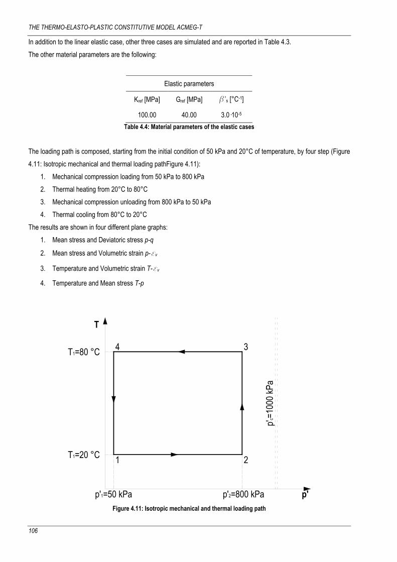
THE THERMO-ELASTO-PLASTIC CONSTITUTIVE MODEL ACMEG-T
106
In addition to the linear elastic case, other three cases are simulated and are reported in Table 4.3.
The other material parameters are the following:
Elastic parameters
Kref [MPa] Gref [MPa] b’s [°C-1]
100.00 40.00 3.010-5
Table 4.4: Material parameters of the elastic cases
The loading path is composed, starting from the initial condition of 50 kPa and 20°C of temperature, by four step (Figure
4.11: Isotropic mechanical and thermal loading pathFigure 4.11):
1. Mechanical compression loading from 50 kPa to 800 kPa
2. Thermal heating from 20°C to 80°C
3. Mechanical compression unloading from 800 kPa to 50 kPa
4. Thermal cooling from 80°C to 20°C
The results are shown in four different plane graphs:
1. Mean stress and Deviatoric stress p-q
2. Mean stress and Volumetric strain p-ev
3. Temperature and Volumetric strain T-ev
4. Temperature and Mean stress T-p
1 2
34
p'1=50 kPa p'2=800 kPa
T1=20 °C
T1=80 °C
p'c=
1000
kPa
p'
T
Figure 4.11: Isotropic mechanical and thermal loading path

CHAPTER 4
107
4.4.2.1 Case 0
0,00
0,05
0,10
0,15
0,20
0,25
0,30
0,35
-0,9 -0,8 -0,7 -0,6 -0,5 -0,4 -0,3 -0,2 -0,1 0,0
Mean stress [MPa]
Dev
iato
ric
stre
ss [M
Pa] COMES-GEO
driver ACMEG-T
Figure 4.12: Mean stress and Deviatoric stress p-q
-0,008
-0,007
-0,006
-0,005
-0,004
-0,003
-0,002
-0,001
0,000
0,001
-0,9 -0,8 -0,7 -0,6 -0,5 -0,4 -0,3 -0,2 -0,1 0,0
Mean stress [MPa]
Volu
met
ric
stra
in [-]
COMES-GEO
driver ACMEG-T
Figure 4.13: Mean stress and Volumetric strain p-eeeev

THE THERMO-ELASTO-PLASTIC CONSTITUTIVE MODEL ACMEG-T
108
-0,008
-0,007
-0,006
-0,005
-0,004
-0,003
-0,002
-0,001
0,000
0,001
0 10 20 30 40 50 60 70 80 90 100
Temperature [°C]
Volu
met
ric
stra
in [-]
COMES-GEO
driver ACMEG-T
Figure 4.14: Temperature and Volumetric strain T-eeeev
-0,90
-0,80
-0,70
-0,60
-0,50
-0,40
-0,30
-0,20
-0,10
0,00
0 10 20 30 40 50 60 70 80 90 100
Temperature [°C]
Mea
n s
tres
s [M
pa]
COMES-GEO
driver ACMEG-T
Figure 4.15: Temperature and Mean stress T-p

CHAPTER 4
109
4.4.2.2 Case 1
0,00
0,05
0,10
0,15
0,20
0,25
0,30
0,35
-0,9 -0,8 -0,7 -0,6 -0,5 -0,4 -0,3 -0,2 -0,1 0,0
Mean stress [MPa]
Dev
iato
ric
stre
ss [M
Pa] COMES-GEO
driver ACMEG-T
Figure 4.16: Mean stress and Deviatoric stress p-q
-0,030
-0,025
-0,020
-0,015
-0,010
-0,005
0,000
-0,9 -0,8 -0,7 -0,6 -0,5 -0,4 -0,3 -0,2 -0,1 0,0
Mean stress [MPa]
Volu
met
ric
stra
in [-]
COMES-GEO
driver ACMEG-T
Figure 4.17: Mean stress and Volumetric strain p-eeeev

THE THERMO-ELASTO-PLASTIC CONSTITUTIVE MODEL ACMEG-T
110
-0,030
-0,025
-0,020
-0,015
-0,010
-0,005
0,000
0 10 20 30 40 50 60 70 80 90 100
Temperature [°C]
Volu
met
ric
stra
in [-]
COMES-GEO
driver ACMEG-T
Figure 4.18: Temperature and Volumetric strain T-eeeev
-0,90
-0,80
-0,70
-0,60
-0,50
-0,40
-0,30
-0,20
-0,10
0,00
0 10 20 30 40 50 60 70 80 90 100
Temperature [°C]
Mea
n s
tres
s [M
pa]
COMES-GEO
driver ACMEG-T
Figure 4.19: Temperature and Mean stress T-p

CHAPTER 4
111
4.4.2.3 Case 2
0,00
0,05
0,10
0,15
0,20
0,25
0,30
0,35
-0,9 -0,8 -0,7 -0,6 -0,5 -0,4 -0,3 -0,2 -0,1 0,0
Mean stress [MPa]
Dev
iato
ric
stre
ss [M
Pa] COMES-GEO
driver ACMEG-T
Figure 4.20: Mean stress and Deviatoric stress p-q
-0,020
-0,015
-0,010
-0,005
0,000
-0,9 -0,8 -0,7 -0,6 -0,5 -0,4 -0,3 -0,2 -0,1 0,0
Mean stress [MPa]
Volu
met
ric
stra
in [-]
COMES-GEO
driver ACMEG-T
Figure 4.21: Mean stress and Volumetric strain p-eeeev

THE THERMO-ELASTO-PLASTIC CONSTITUTIVE MODEL ACMEG-T
112
-0,020
-0,015
-0,010
-0,005
0,000
0 10 20 30 40 50 60 70 80 90 100
Temperature [°C]
Volu
met
ric
stra
in [-]
COMES-GEO
driver ACMEG-T
Figure 4.22: Temperature and Volumetric strain T-eeeev
-0,90
-0,80
-0,70
-0,60
-0,50
-0,40
-0,30
-0,20
-0,10
0,00
0 10 20 30 40 50 60 70 80 90 100
Temperature [°C]
Mea
n s
tres
s [M
pa]
COMES-GEO
driver ACMEG-T
Figure 4.23: Temperature and Mean stress T-p

CHAPTER 4
113
4.4.2.4 Case 3
0,00
0,05
0,10
0,15
0,20
0,25
0,30
0,35
-0,9 -0,8 -0,7 -0,6 -0,5 -0,4 -0,3 -0,2 -0,1 0,0
Mean stress [MPa]
Dev
iato
ric
stre
ss [M
Pa] COMES-GEO
driver ACMEG-T
Figure 4.24: Mean stress and Deviatoric stress p-q
-0,045
-0,040
-0,035
-0,030
-0,025
-0,020
-0,015
-0,010
-0,005
0,000
-0,9 -0,8 -0,7 -0,6 -0,5 -0,4 -0,3 -0,2 -0,1 0,0
Mean stress [MPa]
Volu
met
ric
stra
in [-]
COMES-GEO
driver ACMEG-T
Figure 4.25: Mean stress and Volumetric strain p-eeeev

THE THERMO-ELASTO-PLASTIC CONSTITUTIVE MODEL ACMEG-T
114
-0,045
-0,040
-0,035
-0,030
-0,025
-0,020
-0,015
-0,010
-0,005
0,000
0 10 20 30 40 50 60 70 80 90 100
Temperature [°C]
Volu
met
ric
stra
in [-]
COMES-GEO
driver ACMEG-T
Figure 4.26: Temperature and Volumetric strain T-eeeev
-0,90
-0,80
-0,70
-0,60
-0,50
-0,40
-0,30
-0,20
-0,10
0,00
0 10 20 30 40 50 60 70 80 90 100
Temperature [°C]
Mea
n s
tres
s [M
pa]
COMES-GEO
driver ACMEG-T
Figure 4.27: Temperature and Mean stress T-p
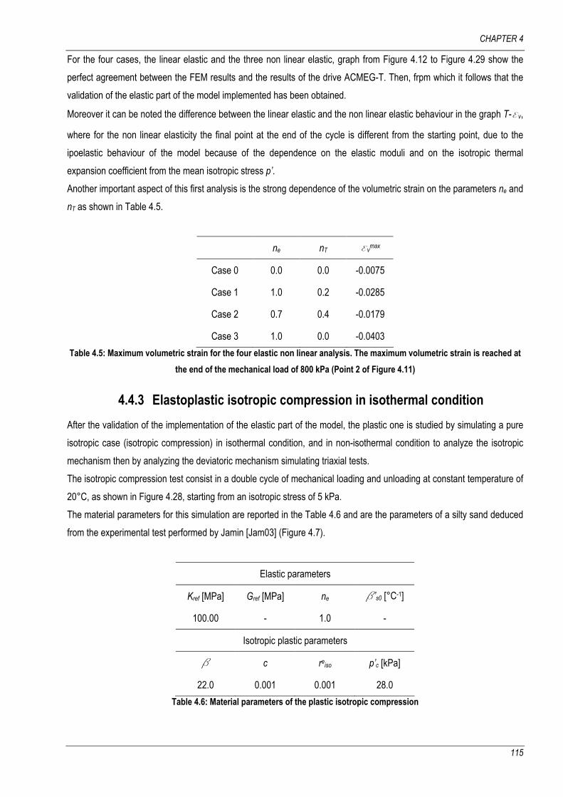
CHAPTER 4
115
For the four cases, the linear elastic and the three non linear elastic, graph from Figure 4.12 to Figure 4.29 show the
perfect agreement between the FEM results and the results of the drive ACMEG-T. Then, frpm which it follows that the
validation of the elastic part of the model implemented has been obtained.
Moreover it can be noted the difference between the linear elastic and the non linear elastic behaviour in the graph T-ev,
where for the non linear elasticity the final point at the end of the cycle is different from the starting point, due to the
ipoelastic behaviour of the model because of the dependence on the elastic moduli and on the isotropic thermal
expansion coefficient from the mean isotropic stress p’.
Another important aspect of this first analysis is the strong dependence of the volumetric strain on the parameters ne and
nT as shown in Table 4.5.
ne nT evmax
Case 0 0.0 0.0 -0.0075
Case 1 1.0 0.2 -0.0285
Case 2 0.7 0.4 -0.0179
Case 3 1.0 0.0 -0.0403
Table 4.5: Maximum volumetric strain for the four elastic non linear analysis. The maximum volumetric strain is reached at
the end of the mechanical load of 800 kPa (Point 2 of Figure 4.11)
4.4.3 Elastoplastic isotropic compression in isothermal condition
After the validation of the implementation of the elastic part of the model, the plastic one is studied by simulating a pure
isotropic case (isotropic compression) in isothermal condition, and in non-isothermal condition to analyze the isotropic
mechanism then by analyzing the deviatoric mechanism simulating triaxial tests.
The isotropic compression test consist in a double cycle of mechanical loading and unloading at constant temperature of
20°C, as shown in Figure 4.28, starting from an isotropic stress of 5 kPa.
The material parameters for this simulation are reported in the Table 4.6 and are the parameters of a silty sand deduced
from the experimental test performed by Jamin [Jam03] (Figure 4.7).
Elastic parameters
Kref [MPa] Gref [MPa] ne b’s0 [°C-1]
100.00 - 1.0 -
Isotropic plastic parameters
b c reiso p’c [kPa]
22.0 0.001 0.001 28.0
Table 4.6: Material parameters of the plastic isotropic compression

THE THERMO-ELASTO-PLASTIC CONSTITUTIVE MODEL ACMEG-T
116
Gref is not necessary for the analysis because the deviatoric mechanism is not activate by the isotropic test. The
coefficient sβ ′ is not necessary because the test is in isothermal condition.
t [s]
p' [kPa]
p'1=77.5 kPa
p'0=5 kPa
p'2=155 kPa
t0=0 s t1=180 s t2=360 s t3=540 s t4=720 s1 3 5
2
4T=20°C
Figure 4.28: Mechanical loading and unloading path
The results of the simulations performed with the F.E. code and with the driver are shown in the p-ev plane (Figure 4.29)
where the good agreement of the results can be observed.
-0,10
-0,09
-0,08
-0,07
-0,06
-0,05
-0,04
-0,03
-0,02
-0,01
0,00
1 10 100 1000
Mean stress [kPa]
Volu
met
ric
stra
in [-]
COMES-GEO
driver ACMEG-T
Figure 4.29: Mean stress and Volumetric strain p-eeeev

CHAPTER 4
117
Moreover, in Figure 4.29 it is possible to compute the value of the material p’c, k and l (see Figure 4.30) and the value
of b.
In fact, from the relation of the volumetric strain vε from the void ratio e
0
0
1 eee
v +−=ε [4.60]
0e results as
0677.110 =
−+=
v
vee
ε
ε [4.61]
Hence from the plotted graph it is possible to compute κ and λ as
( ) ( ) 0026495.0
ln
1ln
1
1
1
00 =
′′
−+=+=
−
−
n
n
nv
nv
pp
ey
xe
εεκ
∆
∆ [4.62]
( ) ( ) 0931369.0
ln
1ln
1
1
1
00 =
′′
−+=+=
−
−
n
n
nv
nv
pp
ey
xe
εελ
∆
∆ [4.63]
1+e0
1+e0
p'c=
28 k
Pa
=0.00147
=0.05172
1 10 100
Mean stress [kPa]
Volu
met
ric
stra
in [-]
-0.005
-0.015
-0.025
-0.035
-0.045
-0.055
Figure 4.30: Graphic extrapolation of p’c, kkkk and llll
From which the parameter β is
85.221 0 =
−+=κλ
βe
[4.64]
similar to the value used in the simulation ( 22=β ).

THE THERMO-ELASTO-PLASTIC CONSTITUTIVE MODEL ACMEG-T
118
The difference between the imposed value and the extrapolated one is due to the imprecision of the slope of the two
lines of the graph due to the effect of the very small value of reiso on the elastic and the plastic curves of Figure 4.30.
Additionally the experimental test performed by Jamin [Jam03] was simulated and the results of the numerical
simulations are showed together with the experimental results (Figure 4.31).
-0,15
-0,13
-0,11
-0,09
-0,07
-0,05
-0,03
-0,01
1 10 100 1000
Mean stress [kPa]
Volu
met
ric
stra
in [-]
COMES-GEO
driver ACMEG-T
Jamin 2003
Figure 4.31: Comparison between numerical results by COMES-GEO and driver ACMEG-T and experimental results by
Jamin [Jam03]
Also for this simulation, as for the elastic one, the finite element results of COMES-GEO coincide with those of the driver
ACMEG-T.
From the simulations of sections 4.4.2and 4.4.3 it can be concluded that the isotropic mechanism is validate.
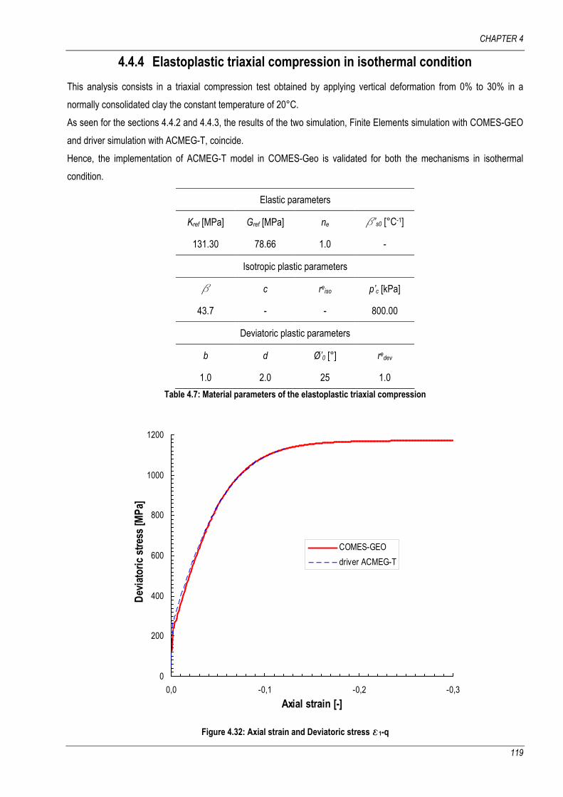
CHAPTER 4
119
4.4.4 Elastoplastic triaxial compression in isothermal condition
This analysis consists in a triaxial compression test obtained by applying vertical deformation from 0% to 30% in a
normally consolidated clay the constant temperature of 20°C.
As seen for the sections 4.4.2 and 4.4.3, the results of the two simulation, Finite Elements simulation with COMES-GEO
and driver simulation with ACMEG-T, coincide.
Hence, the implementation of ACMEG-T model in COMES-Geo is validated for both the mechanisms in isothermal
condition.
Elastic parameters
Kref [MPa] Gref [MPa] ne b’s0 [°C-1]
131.30 78.66 1.0 -
Isotropic plastic parameters
b c reiso p’c [kPa]
43.7 - - 800.00
Deviatoric plastic parameters
b d Ø’0 [°] redev
1.0 2.0 25 1.0
Table 4.7: Material parameters of the elastoplastic triaxial compression
0
200
400
600
800
1000
1200
-0,3-0,2-0,10,0
Axial strain [-]
Dev
iato
ric
stre
ss [M
Pa]
COMES-GEO
driver ACMEG-T
Figure 4.32: Axial strain and Deviatoric stress eeee1-q

THE THERMO-ELASTO-PLASTIC CONSTITUTIVE MODEL ACMEG-T
120
-0,030
-0,025
-0,020
-0,015
-0,010
-0,005
0,000
-0,3-0,2-0,10,0
Axial strain [-]
Volu
met
ric
stra
in [-]
COMES-GEO
driver ACMEG-T
Figure 4.33: Axial strain and Volumetric strain eeee1-eeeev
Therefore, the next analysis will be done with the aim to validate the model in non-isothermal conditions.
4.4.5 Elastoplastic isotropic compression in non-isothermal condition
For the validation of the isotropic mechanism in non-isothermal conditions, an isotropic compression is performed by
applaying a thermal cycle. Starting from the ambient temperature of 21.5 °C, the sample is heated until the temperature
of 95 °C and then cooled until the initial temperature, 21.5 °C (Figure 4.34).
The material parameters are reported in the Table 4.8 and are those of a Boom clay.
Elastic parameters
Kref [MPa] Gref [MPa] ne b’s0 [°C-1]
150.00 130.00 0.4 3.010-5
Isotropic plastic parameters
b c reiso p’c [MPa] gT
47.0 0.0004 0.01 6.0 0.18
Table 4.8: Material parameters of Boom clay
The test is repeat for three times for three different degree of consolidation: OCR=1, OCR=2 and OCR=6.

CHAPTER 4
121
1
2
3T1=21.5 °C
T1=95 °C
T
t0=0 s t [s]t1=200 s t2=400 s
Figure 4.34: Thermal path of heating and cooling
The results of the simulation are shown in the ev-T plane, three simulation are shown in Figure 4.35 to outline the
behaviour of normal consolidated clay (OCR=1) that contracts with the increase of temperature, while on the contrary,
the overconsolidate clay (OCR=6) dilates. Figure 4.35 show also the other main aspect of the behaviour of clays under
heating which is the irreversible dilatant deformation for NC clays.
20
30
40
50
60
70
80
90
100
-0,3% -0,2% -0,1% 0,0% 0,1% 0,2%
Volumetric strain [-]
Tem
per
ature
[°C
]
COMES-GEO
driver ACMEG-TOCR=1
OCR=2
OCR=6
Figure 4.35: Volumetric strain and Temperature eeeev-T

THE THERMO-ELASTO-PLASTIC CONSTITUTIVE MODEL ACMEG-T
122
In the following graph there is the comparison between the results of the finite element simulation with COMES-GEO
and the experimental results obtained by Baldi [Bal91] on Boom clay for OCR=1 and OCR=2.
20
30
40
50
60
70
80
90
100
-0,25% -0,20% -0,15% -0,10% -0,05% 0,00% 0,05%
Volumetric strain [-]
Tem
per
ature
[°C
]COMES-GEO
EXPERIMENTALOCR=1
OCR=2
Figure 4.36: Comparison between finite element COMES-GEO and experimental results obtained by Baldi et al. [Bal91] on
Boom clay for OCR=1 and OCR=2

CHAPTER 4
123
4.5 A NON ISOTHERMAL CONSOLIDATION EXAMPLE†
In this section a case of non-isothermal elastic and elasto-plastic consolidation is studied.
The following example aims to validate the finite element formulation solving an initial boundary value problem. It deals
with the simulation of a non-isothermal fully saturated consolidation problem, for which the numerical solution of the
linear thermo-mechanical problem is known [Abo85].
A column of 7 m height and 2 m width is subjected to an external surface compressive load of 1.0 kPa and to a surface
temperature jump of 50 K above the initial ambient temperature of 293.15 K. The material is initially water saturated. The
upper surface is drained (pw = 0 Pa); the lateral and the bottom surfaces are insulated. Horizontal displacements are
constrained along the vertical boundaries and vertical displacements are constrained at the bottom surface. The column
is discretized by nine eight-node isoparametric elements Figure 4.37. Furthermore, 3×3 Gauss integration points are
used. The material parameters used in the computation are listed in Table 4.9. Gravity forces are taken into account.
Plane strain conditions are assumed.
Figure 4.37: Spatial discretization and boundary conditions for the non-isothernal consolidation example
† This section is reproduced from: Sanavia L., François B., Bortolotto R., Luison L., Laloui L. (2008). Finite element modelling of
thermo-elasto-plastic water saturated porous materials. Journal of Theoretical and Applied Mechanics, 38, 1-2, pp 7-34.

THE THERMO-ELASTO-PLASTIC CONSTITUTIVE MODEL ACMEG-T
124
Elastic parameters
Kref [MPa] Gref [MPa] ne b’s0 [°C-1]
10.0 2.14 0 9.010-7
Isotropic plastic parameters
b c reiso p’c [kPa] gT
20.0 0.001 0.001 800.00 0.2
Diffusive law parameters
rs [kg/m³] n k [m²] ls [W/(mK)] cs [J/(kgK)] lw [W/(mK)] cw [J/(kgK)]
2000 0.2 4.610-17 0.84 16760 0.6 4181
Table 4.9: Material parameters for Aboustit example
The case studied in [Abo85], which assumed constant Young modulus (E = 6.0 MPa) and Poisson ratio (n = 0.4) and
constant cubic thermal expansion coefficient, is here used as validation example. To this aim, the results of [Abo85] as
published in [L&S98] and labelled “Aboustit” in the Figure 4.38 to Figure 4.43, are used to compare the solution obtained
with the finite element formulation proposed in this chapter and labelled “COMES-GEO”. The time histories for the water
pressure (Figure 4.38), the temperature (Figure 4.39) and the vertical displacement (Figure 4.40) of several nodes of the
mesh show the coincidence of the two solutions. The linear behaviour of the thermo-mechanical problem adopting the
ACMEG-T model is obtained by using the mechanical moduli independent of the stress state (ne = 0).
As shown all along the present chapter, soils are often subject to irreversible processes induced by thermal effect. In this
context, the last simulation extends the problem of Figure 4.37 towards elasto-thermoplastic analysis. The material
parameters are listed in Table 4.9, where it can be observed that the linear elasticity is kept for comparison with the
previous simulation; thermo-plasticity is introduced by reducing the preconsolidation pressure to get a mechanical and
thermal hardening when loaded to 1kPa and introducing the decrease of the isotropic yield surface with temperature.
The comparison between the elastic and the elasto-plastic solution shows that the inclusion of the plasticity effects
delays the dissipation of pore water pressure in time (Figure 4.41), because of the reduced thermo-plastic stiffness of the
solid skeleton with respect to the elastic one. Moreover, the predicted water pressures at the same time station are
therefore higher than those from the elastic analysis.
Temperature evolution is almost not modified with respect to the previous simulation, as it can be observed in Figure
4.42. Indeed, because parameters of thermal conduction and convection are almost independent on porosity changes,
at least for this range of volumetric strain, [2.190] remains almost unaffected by mechanical change. On the contrary, the
time history for the vertical displacements appears to be strongly affected by the thermo-plastic behaviour of the solid
skeleton. In particular, an increase of two order of magnitude for the vertical displacements is observed in Figure 4.43,
that makes negligible the thermal component that can be observed in Figure 4.40.

CHAPTER 4
125
-1100
-1000
-900
-800
-700
-600
-500
-400
-300
-200
-100
0
100
1,E-02 1,E-01 1,E+00 1,E+01 1,E+02 1,E+03 1,E+04 1,E+05 1,E+06
Time [day]
Pore
wat
er p
ress
ure
[P
a]
3 COMES-GEO
6 COMES-GEO
12 COMES-GEO
22 COMES-GEO
40 COMES-GEO
45 COMES-GEO
3 Aboustit
6 Aboustit
12 Aboustit
22 Aboustit
40 Aboustit
45 Aboustit
Figure 4.38: Elastic case: Evolution of pore water pressure
290
300
310
320
330
340
350
1,E-02 1,E-01 1,E+00 1,E+01 1,E+02 1,E+03 1,E+04 1,E+05 1,E+06
Time [day]
Tem
per
ature
[K
]
3 COMES-GEO
6 COMES-GEO
12 COMES-GEO
22 COMES-GEO
40 COMES-GEO
45 COMES-GEO
3 Aboustit
6 Aboustit
12 Aboustit
22 Aboustit
40 Aboustit
45 Aboustit
Figure 4.39: Elastic case: Evolution of temperature

THE THERMO-ELASTO-PLASTIC CONSTITUTIVE MODEL ACMEG-T
126
-5,E-04
-4,E-04
-3,E-04
-2,E-04
-1,E-04
0,E+00
1,E-04
1,E-02 1,E-01 1,E+00 1,E+01 1,E+02 1,E+03 1,E+04 1,E+05 1,E+06
Time [day]
Ver
tica
l dis
pla
cem
ent [m
]
3 COMES-GEO
6 COMES-GEO
12 COMES-GEO
22 COMES-GEO
40 COMES-GEO
45 COMES-GEO
3 Aboustit
6 Aboustit
12 Aboustit
22 Aboustit
40 Aboustit
45 Aboustit
Figure 4.40: Elastic case: Evolution of vertical displacement
-1200
-1100
-1000
-900
-800
-700
-600
-500
-400
-300
-200
-100
0
100
1,E-02 1,E+00 1,E+02 1,E+04 1,E+06 1,E+08
Time [day]
Pore
wat
er p
ress
ure
[P
a]
3 COMES-GEO
6 COMES-GEO
12 COMES-GEO
22 COMES-GEO
40 COMES-GEO
45 COMES-GEO
3 Aboustit
6 Aboustit
12 Aboustit
22 Aboustit
40 Aboustit
45 Aboustit
Figure 4.41: Elastoplastic case: Evolution of pore water pressure

CHAPTER 4
127
290
300
310
320
330
340
350
1,E-02 1,E+00 1,E+02 1,E+04 1,E+06 1,E+08
Time [day]
Tem
per
ature
[K
]3 COMES-GEO
6 COMES-GEO
12 COMES-GEO
22 COMES-GEO
40 COMES-GEO
45 COMES-GEO
3 Aboustit
6 Aboustit
12 Aboustit
22 Aboustit
40 Aboustit
45 Aboustit
Figure 4.42: Elastoplastic case: Evolution of temperature
-4,E-02
-3,E-02
-2,E-02
-1,E-02
0,E+00
1,E-02
1,E-02 1,E+00 1,E+02 1,E+04 1,E+06 1,E+08
Time [day]
Ver
tica
l dis
pla
cem
ent [m
] 3 COMES-GEO
6 COMES-GEO
12 COMES-GEO
22 COMES-GEO
40 COMES-GEO
45 COMES-GEO
3 Aboustit
6 Aboustit
12 Aboustit
22 Aboustit
40 Aboustit
45 Aboustit
4
Figure 4.43: Elastoplastic case: Evolution of vertical displacement

THE THERMO-ELASTO-PLASTIC CONSTITUTIVE MODEL ACMEG-T
128
References
[Abo85] Aboustit B.L., Advani S.H. and Lee J.K. (1985). Variational principles and finite element simulations for
thermo-elastic consolidation. International Journal for Numerical and Analytical Methods in Geomechanics,
9: 49-69.
[A-N05] Abuel-Naga H.M. (2005). Thermo-mechanical behaviour of soft Bangkok Clay: experimental results and
constitutive modelling. PhD Thesis, Asian Institute of Technology, Bangkok, Thailand.
[A-N06] Abuel-Naga H.M., Bergado D.T., Ramana G.V., Grino L., Rujivipat P. and Thet Y. (2006). Experimental
evaluation of engineering behaviour of soft Bangkok clay under elevated temperature. Journal of
Geotechnical and Geoenvironmental Engineering, 132(7): 902-910.
[A-N07] Abuel-Naga H.M., Bergado D.T. and Bouazza A. (2007). Thermally induced volume change and excess
pore water pressure of soft Bangkok clay. Engineering Geology, 89(1-2): 144-154.
[Bal91] Baldi G., Hueckel T., Peano A. and Pellegrini R. (1991). Developments in modelling of thermohydro-
mechanical behaviour of Boom clay and clay-based buffer materials (Vol 1 and 2). EUR 13365/1 and
13365/2, Luxembourg.
[Bur00] Burghignoli A., Desideri A. and Miliziano S. (2000). A laboratory study on the thermomechanical behaviour
of clayey soils. Canadian Geotechnical Journal, 37: 764-780.
[C&L04] Cekerevac C. and Laloui L. (2004). Experimental study of thermal effects on the mechanical behaviour of a
clay. International Journal for Numerical and Analytical Methods in Geomechanics, 28(3): 209-228.
[C&M68] Campanella R.G. and Mitchell J.K. (1968). Influence of temperature variations on soil behaviour. Journal of
the Soil Mechanics and Foundation Division, ASCE, 94: 709-734.
[Cek03] Cekerevac C. (2003). Thermal effect on the mechanical behaviour of saturated clays: an experimental and
constitutive study. PhD Thesis. École Polytechnique Fédérale De Lausanne. Suisse.
[D&C82] Demarks K.R. and Charles R.D. (1982). Soil volume changes induced by temperature cycling. Canadian
Geotechnical Journal, 19: 188-194.
[DeO96] Del Olmo C., Fioravante V., Gera F., Hueckel T., Mayor J.C. and Pellegrini R. (1996). Thermomechanical
properties of deep argillaceous formations. Engineering Geology, 41: 87-102.
[Fra08] François B. (2008). Thermo-Plasticity of Fine-Grained Soils at Various Saturation States: Application to
Nuclear Waste Disposal. PhD Thesis. École Polytechnique Fédérale De Lausanne. Suisse.
[H&P89] Hueckel T. and Pellegrini R. (1989). Modelling of thermal failure of saturated clays. International Symposium
on Numerical Models in Geomechanics – NUMOG: 81-90.
[Hue98] Hueckel T., Pellegrini R. and Del Olmo C. (1998). A constitutive study of thermo-elasto-plasticity of deep
carbonatic clays. International Journal of Numerical and Analytical Methods in Geomechanics, 22: 549-574.
[Huj79] Hujeux J.C. (1979). Calcul numérique de problèmes de consolidation élastoplastique. PhD Thesis, Ecole
Centrale, Paris.
[Huj85] Hujeux J.C. (1985). Une loi de comportement pour le chargement cyclique des sols. Génie Parasismique,
Les éditions de l'E.N.P.C., Paris: 287-303.
[Jam03] Jamin F. (2003). Contribution à l'étude du transport de matière et de la rhéologie dans les sols non saturés
à différentes températures. PhD Thesis. Université Montpellier II.

CHAPTER 4
129
[Kin76] Kingery W.D, Bowen H.K. and Uhlmann D.R. (1976). Introduction to Ceramics, 2nd Edition. Wiley, New
York.
[Kun95] Kuntiwattanakul P., Towhata I., Ohishi K. and Seko I. (1995). Temperature effects on undrained shear
characteristics of clay. Soils and Foundations, 35(1): 147-162.
[L&C03] Laloui L. and Cekerevac C. (2003). Thermo-plasticity of clays: An isotropic yield mechanism, Computers
and Geotechnics, 30(8): 649-660.
[L&C08] Laloui L. and Cekerevac C. (2008). Non-isothermal plasticity model for cyclic behaviour of soils.
International Journal for Numerical and Analytical Methods in Geomechanics, 32(5): 437-460.
[L&F08] Laloui L. and François B. (2009) ACMEG-T: A soil thermo-plasticity model. Journal of Engineering
Mechanics. DOI: 10.1061/(ASCE)EM.1943-7889.0000011.
[L&S98] Lewis R.W. and Schrefler B.A. The Finite Element Method in the Static and Dynamic Deformation and
Consolidation of Porous Media. J. Wiley, Chichester 1998.
[Lal01] Laloui L. (2001). Thermo-mechanical behaviour of soils. Environmental Geomechanics. EPFL Press,
Lausanne: 809-843.
[Lal05] Laloui L., Cekerevac C. and François B. (2005) Constitutive modelling of the thermo-plastic behaviour of
soils. Revue Européenne de Génie Civil, 9(5-6): 635-650.
[Lal93] Laloui L. (1993). Modélisation du comportement thermo-hydro-mécanique des milieux poreux anélastique.
PhD Thesis, Ecole Centrale de Paris.
[M&L97] Modaressi H. and Laloui L. (1997). A thermo-viscoplastic constitutive model for clays. International Journal
for Numerical and Analytical Methods in Geomechanics, 21(5): 313–315.
[N&W79] Nova R. and Wood D.M. (1979). A constitutive model for sand in triaxial compression. International Journal
for Numerical and Analytical Methods in Geomechanics, 3: 255–278.
[Pra49] Prager W. (1949). Recent developments in mathematical theory of plasticity. Journal of Applied Physics,
20(3): 239-241.
[Pra58] Prager W. (1958). Non-isothermal plastic deformation. Koninkklijk-Nederland Akademie Van
Wetenschappen Te Amsterdam - Proceedings of the section of sciences- B, 61, 176-182.
[Pus87] Pusch R. (1987). Permanent crystal lattice contraction, primary mechanism in thermally induced alteration
of Na-bentonite. Scientific Basis for Nuclear Waste Management X. MRS, Pittsburgh, 84: 792 802.
[Riz96] Rizzi E., Maier G. and Willam K. (1996). On failure indicators in multi-dissipative materials. International
Journal of Solids and Structures, 33(20-22): 3187-3214
[San08] Sanavia L., François B., Bortolotto R., Luison L., Laloui L. (2008). Finite element modelling of thermo-elasto-
plastic water saturated porous materials. Journal of Theoretical and Applied Mechanics, 38, 1-2, pp 7-34.


CHAPTER 5
131
5 THE THERMO-HYDRO-ELASTO-PLASTIC CONSTITUTIVE
MODEL ACMEG-TS
5.1 PARTIAL SATURATION IN SOIL
Most soils in nature are in condition of partial saturation, and hence is of fundamental importance the development of
constitutive model able to take into account the effects of this state.
As explained in the previous sections, the soils are composed by a solid porous skeleton with voids. The voids can be
filled with water, and soils are said fully saturated, or can be filled with water and air, and soils in this case are defined as
unsaturated or partially saturated. If in a saturated soil the pore fluid pressure can generally be assumed as a neutral
stress, on the contrary, under unsaturated conditions, a new internal stress, namely the suction, s, or the capillary
pressure, pc, (seen in chapter 2), plays a significant role in the behaviour of unsaturated soils and must be, directly or
indirectly, considered in the formulation of the stress-strain relationship. The relative amounts of the pore air and pore
water phases play a key role in the mechanical properties of the unsaturated soils. This proportion, usually defined by
the degree of saturation, Sw, should be considered, directly or indirectly, in the complete description of the hydro-
mechanical soil state.
The degree of saturation is defined as (see 2.6.1):
gw
w
w dvdvdv
S+
= [5.1]
where dvw is the volume of voids filled with water
dvg is the volume of voids filled with the air phase, that can be assumed to be a mixture of dry air and vapour
Sw is connected to the pc through experimental laws that was proposed during the years from some authors as shown in
5.3.
As seen in 2.6, for unsaturated soils we need of an appropriate definition of the effective stress.
Starting from the well known relationship by Terzaghi [Ter36]
ijw
ijij p δσσ −=′ [5.2]
the effective stress ijσ ′ must used for unsaturated soils has been proposed by Bishop [2.155] is
ijc
ijnetijwg
ijg
ijij pppp δχσδχδσσ ⋅+=−+−=′ , )( [5.3]
where ijg
ijijnet p δσσ −=,
wgc ppp −=
As shown in 2.6.1, equation [2.162], we assume that
wS=χ [5.4]

THE THERMO-HYDRO-ELASTO-PLASTIC CONSTITUTIVE MODEL ACMEG-TS
132
as proposed by Schrefler [Sch84].
Others authors proposed expressions for c which depend on a suction ratio rather than on the degree of saturation
[Ait60] [K&K98]. From a micromechanical standpoint, theoretical approaches were also developed to evaluate the c
parameter by examining the forces and fluid pressures that arise in unsaturated soils with idealized soil particles. That
kind of analysis shows that the shape and the arrangement of grains, as well as the contact angle at the solid-liquid
interface, may have a significant impact on the behaviour of the c parameter [L&L04].
Figure 5.1: Effective stress parameter with respect to the degree of saturation for various soils, as reported in [Zer91]. Here
Sr is the notation used for the degree of saturation. (Redrawn from [Fra08]).
5.1.1 Mechanical behaviour
This section presents the stress-strain behaviour of unsaturated soils under isothermal conditions [Fra08]. It will be
shown that the mechanical response of partially saturated soils is significantly affected by the soil suction. The
characterization of the mechanical response of unsaturated soils depends strongly on the stress reference used in the
representation of the experimental results. The curves obtained from laboratory tests are usually displayed according to
net stresses because they are the direct data monitored during the experiments. This provides a consistent framework to
analyse the obtained results. However, the pseudo-effective stress approach may bring substantial clarification to some
observed features of soil behaviour. Therefore, where possible in this section, the experimental results will be presented
using the Bishop-type effective stress with c=Sw , called the generalized effective stress (Nuth and Laloui [N&L08]), in
parallel with the net stress. This interpretation is possible only if the water retention information is available.
5.1.1.1 Effect of suction on the compressive behaviour in isothermal conditions
The apparent preconsolidation pressure increases remarkably upon desaturation. This increase of the elastic domain
with suction is narrowly linked to capillary effects. During a consolidation process, the yield limit corresponds to the

CHAPTER 5
133
stress level that begins to produce a rearrangement of particles. As suction increases, air enters in pores and the
menisci that form at the air-water interface stabilize the particle-particle contact. This stabilizing effect pushes back the
soil yielding limit.
Figure 5.2: Evolution of the yielding limit with respect to suction determined from oedometric compression tests on
compacted Boom clay at ambient temperature [Rom99] (redrawn from [Fra08])
Figure 5.2 shows the evolution of the preconsolidation pressure with suction, as determined from compression tests on
compacted Boom clay in both net stress and generalized effective stress [Rom99]. The evolution of the preconsolidation
pressure appears to be rapid for low values of suction and then becomes asymptotic for higher ones. The Figure 5.2
also shows that the increase in the elastic limit is noticeable only for suction higher than a given limit suction, the air-
entry suction, which is the capillary pressure value at which air begins to enter the pores. Above this limit, a logarithmic
function might be suitable to model this phenomenon. Based on its similarity with the temperature effect and the
evolution law proposed by Laloui and Cekerevac [L&C03], Nuth and Laloui [N&L07] proposed the same logarithmic
formulation to quantify the one-to-one relationship between suction and the preconsolidation pressure in the generalized
effective stress reference:
+=⇒>
=⇒≤
eScce
cce
ss
p'sp'ss
p'sp'ss
log1)(
)(
0
0
γ [5.5]
where 0cp′ is the preconsolidation pressure at saturation
( )spc′ is the preconsolidation pressure at a given suction s
se is the air-entry suction
gs is a material parameter

THE THERMO-HYDRO-ELASTO-PLASTIC CONSTITUTIVE MODEL ACMEG-TS
134
In the saturated domain (i.e. for suction lower than the air-entry suction value), equation [5.5] assumes that a positive
suction can take place without affecting directly the preconsolidation pressure, which remains equal to its value in fully
saturation condition, provided that no volumetric plastic strains are produced during the suction evolution.
Figure 5.3 shows the logarithmic law [5.5] compared with the experimental data referred to two different soil type.
Figure 5.3: Comparison between experimental data and value predicted by the law [5.5]. a) Oedometric test on Boom clay
[Rom99] b) Isotropic compression test on Sion silt [Gei99]. (Redrawn from [Fra08]).
5.1.1.2 Effect of suction on the compressive behaviour in non-isothermal conditions
In addition to the observed behaviour of unsaturated soils at ambient temperature and of saturated soils under non-
isothermal conditions, some coupled effects between suction and temperature arise in soils when unsaturated and non-
isothermal conditions are simultaneously met. These interactions must be considered in the development of constitutive
models in order to cover the range of thermo-hydro-mechanical couplings occurring in fine-grained soils. These coupling
effects, experimentally observed on compression and wetting-drying paths, are described in the following sections.
From experimental programs studying the thermal and the suction effects on the compressive behaviour of soils
separately, the experimental results clearly show a decrease of the preconsolidation pressure with temperature and an
increase with suction.
However, the combined effects of temperature and suction on the preconsolidation pressure lacks of confirmation. On
compacted Boom clay loaded under oedometric conditions, Romero [Rom99] noticed a very small effect due to
temperature, regarding the suction effect, on the evolution of the preconsolidation pressure (Figure 5.4 a). However, the
results confirm the usual decreases of p’c with temperature and its increases with suction. Tang et al. [Tan08] observed
similar behaviour on MX80 bentonite (Figure 5.4 b).

CHAPTER 5
135
Figure 5.4: Effect of temperature and suction on the yield limit. a) Oedometric test on Boom clay [Rom99] b) Isotropic
compression test on MX80 bentonite [Tan08]. (Redrawn from [Fra08]).
5.1.2 Conclusion
For a more complete description of the experimental behaviour of partially saturated soils, in isothermal and non-
isothermal conditions, the interested reader can refers to the Phd thesis of Francois [Fra08] at which part of this chapter
is referred.
In particulary, in the second part of this thesis is presented the influence of temperature on the hydro-mechanical
response of unsaturated soils. The analysis performed in the thesis show the strong link between the mechanical and
the water retention behaviour. Hence, because temperature affects both the stress-strain and degree of saturation-
suction relationships, temperature plays an important role in the global response of unsaturated soils.
In particular, the generated plastic strains upon various thermo-hydro-mechanical paths have been shown to be closely
related to the temperature and suction of the soil. Among other examples, the collapse propensity of a soil, occurring
upon soil humidification, is not only affected by the external stress level but also by temperature. Similarly, the elastic
domain is enhanced with increasing suction, while it decreases with increasing temperature. This has conseguences in
terms of volumetric strains, which implies modification of the water retention capability of unsaturated soil. In fact, the
water retention curve is affected by the mechanical state of the soil and by the temperature [Fra08]. The denser the soil,
the higher its degree of saturation for an equivalent suction. On the other hand, temperature tends to reduce the degree
of saturation at a given suction. This behaviour has to be taken into account in a constitutive model, as it has been
proposd in section 5.3.

THE THERMO-HYDRO-ELASTO-PLASTIC CONSTITUTIVE MODEL ACMEG-TS
136
5.2 ACMEG-TS MODEL‡
5.2.1 Isotropic plastic mechanism
Similarly to equation [4.14], the yield limit, fiso, of the isotropic plastic mechanism is expressed by :
0=⋅′−′= isociso rppf [5.6]
where isor is the degree of mobilization of the isotropic mechanism.
The enhancement of the isotropic elastic domain with increasing suction is introduced through the evolution of the
preconsolidation pressure p’c Figure 5.5. As experimentally observed, the evolution of p’c with combined temperature T
and suction s can be expressed by a logarithmic function [F&L08]
+
−=⇒>
−=⇒≤
esTc
pvce
Tcpvce
ss
TT
p'Tsp'ss
TT
p'Tsp'ss
log1log1),,(
log1),,(
00
00
γγε
γε
[5.7]
Figure 5.5: a) Evolution of the isotropic yield limit with suction at difference temperatures; b) dependence of the isotropic
yield limit on the ggggs parameter. (Redrawn from [Fra08]).
In addition, the mechanical hardening produces an evolution of the preconsolidation pressure with the generated
volumetric plastic strain and hence the thermo-hydro-mechanical evolution of the preconsolidation pressure is expressed
as
+
−⋅=⇒>
−⋅=⇒≤
⋅
⋅
esTc
pvce
Tcpvce
ss
TT
ep'Tsp'ss
TT
ep'Tsp'ss
pv
pv
log1log1),,(
log1),,(
00
00
γγε
γε
εβ
εβ
[5.8]
‡ Refernce [F&L08]

CHAPTER 5
137
where 0cp′ is the preconsolidation pressure in fully saturation conditions and at temperature T0
cp′ is the preconsolidation pressure at a given suction s and at the reference temperature T
se is the air-entry suction
gs is a material parameter for the dependence of preconsolidation pressure on s
gT is a material parameter for the dependence of preconsolidation pressure on T
b is the plastic compressibility modulus (the slope of the linear function in the pvε - ln p’c plane)
The flow rule for the isotropic mechanism is given by equation [4.23].
5.2.2 Deviatoric plastic mechanism
Similarly to equation [4.24], the yield limit, fdev, of the deviatoric plastic mechanism is expressed by Hujeux [Huj79]:
0ln1 =⋅
′′⋅⋅−′−= dev
cdev r
ppd
bpMqf [5.9]
where Φ
ΦM=
′−′
sin3sin6
is the slope of the critical state line (CSL) in the p’-q plane
pd
pde
devdev arr
ε
ε
++= is the degree of plastification of the deviatoric mechanism
Φ′ is the friction angle at critical state
b is a material parameter defining the shape of the deviatoric yield limit
d is the ratio between the preconsolidation pressure, p’c, and the critical pressure, p’cr.
The ACMEG-TS model assumes that the friction angle may depend on temperature by the equation
( )00 TTgMM −−= [5.10]
where M0 is the is the slope of the critical state line at ambient temperature T0
g is an average slope of variation of friction angle at critical state with temperature
but remains unaffected by suction change in the generalized effective stress reference, as noticed by Nuth and Laloui
[N&L08].
The hardening and dilatancy rules of the deviatoric mechanism are expressed by equations [4.25] to [4.29].
5.2.3 Coupling between the two plastic mechanisms
The shape of the elastic domain follows from the combinations of the deviatoric yield limit [4.47] with the thermo-hydro-
mechanical evolution of the preconsolidation pressure [5.8]. Figure 5.6 [F&L08] [Fra08] illustrates the effect of suction,
temperature and generated volumetric plastic strain on the evolution of the elastic domain.
It must be noted that the temperature and suction dependence of the isotropic yield limit is a one-to-one relationship.
Provided that the stress point remains in the elastic domain, a suction and/or a temperature cycle does not modify the
final preconsolidation pressure with respect to the initial one, if the final state is identical to the initial one. On the
contrary, the volumetric plastic strain produces irreversible modification of the isotropic yield limit. In other words, the
volumetric plastic strain is a hardening variable, while temperature and suction are not.

THE THERMO-HYDRO-ELASTO-PLASTIC CONSTITUTIVE MODEL ACMEG-TS
138
The coupling between the two plastic mechanisms is similar to that in the ACMEG-T model under saturated conditions.
However, inclusion of the derivative of the yield limits with respect to suction is required in the consistency conditions for
multi-mechanism [4.50] due to the evolution of both yield limits with suction level. The consistency condition of the two
yielding mechanisms must be met simultaneously, requiring solution of two equations with two unknowns.
Figure 5.6: Effect of (a) suction, (b) temperature and (c) volumetric plastic strain on the shape of coupled mechanical yield
limits [F&L08]. (Redrawn from [Fra08]).

CHAPTER 5
139
0
0
0::
=⋅≥
≤⋅−⋅+⋅+′=⋅∂∂⋅
∂∂+⋅
∂∂+⋅
∂∂+′
′∂∂=
p
p
ppp
d
dTdsddTT
dss
dd
λ
λ
λλλ
π
π
F
HtiσjFFF
σσ
FF
[5.11]
where σ′ is the generalized effective stress vector
p is the internal variable tensor
j collects the stress-gradient
t is the temperature-gradient of the loading function F
H is the matrix of hardening moduli p
f
β
ααβ λ∂
∂−=H
pλ is the plastic multiplier vector
0≤Fd expresses Prager’s consistency condition extended to multiple dissipation processes
i collects the suction-gradient of the loading function
In the framework of generalized effective stress, Borja [Bor04] proved that including suction in the argument of the yield
functions is motivated by thermodynamic considerations.
Within the adopted generalized stress framework, σ′ depends on s, which makes these two state variables dependent.
In order to avoid the two effects of the suction increment (in σ′d and ds itself) in the consistency equation, numerical
integration at the local (Gauss point) level is performed by considering suction fixed at its final value during the plastic
corrector phase. In other words, as suggested by Borja, there is no return map on the suction axis during numerical
integration of the model, which makes ds equal to zero in equation [5.11]. Hence, there is no change in the consistency
relations with respect to the saturated model, excepted that, at each time step, the value of the preconsolidation
pressure is calculated considering the suction at the end of the time step through equation [5.8].

THE THERMO-HYDRO-ELASTO-PLASTIC CONSTITUTIVE MODEL ACMEG-TS
140
5.3 WATER RETENTION CONSTITUTIVE PART
In 2.4.5 we have seen that the pore size distribution is dependent on the capillary pressure, the temperature and the
volumetric strain.
In this section we will summarize the relationship between the degree of saturation Sw and suction s taking into account
also the influence of temperature and usually neglected volumetric strain, following [Fra08].
( )vc TpSS εππ , ,= [5.12]
Generally speaking all the relationship that can be found in literature are derived from experimental data (see Figure 5.7
and Table 5.1).
For this work the following relationship are used and are called Brooks and Corey, Safai and Pinder (from the name of
the authors that have proposed them) and ACMEG-HYDRO (from the name of the model where this law is shown
[Fra08]).
These relationship are summarize in the following togheter with their derivatives necessary for the Jacobian matrix after
linearization of the discretized governing equations (see 3.1.2.2).
0,00
0,10
0,20
0,30
0,40
0,50
0,60
0,70
0,80
0,90
1,00
1,10
0 1 10 100 1000
Suction [MPa]
Deg
ree
of sa
tura
tion [-]
Figure 5.7: Experimental data (from Lyesse Laloui with personal communication)

CHAPTER 5
141
S [MPa] Sw
0,50 0,972
1,00 1,00
0,983 1,041
4,12 4,12 4,12
0,951 0,931 0,944
20,41 20,41 20,41
0,510 0,539 0,531
37,13 37,13 37,13
0,369 0,407 0,428
80,89 80,89 80,89
0,365 0,315 0,348
111,08 111,08 111,08
0,256 0,242 0,260
150,00 150,00 150,00
0,235 0,221 0,196
286,86 286,86 286,86
0,078 0,115 0,103
325,79 325,79 325,79
0,056 0,064 0,049
Table 5.1: Experimental data
5.3.1 Brooks and Corey
The relation proposed by Brooks and Corey [B&C64] is the follow
( )λ
−+
−+==
bref
irrirrww
pps
SSsSS
1
1 [5.13]
where Sirr is the irreducible degree of saturation
λ is the index of the pore size distribution which is defined as the negative slope of the effective Sw
pref is the reference pressure
pb is the bubble pressure

THE THERMO-HYDRO-ELASTO-PLASTIC CONSTITUTIVE MODEL ACMEG-TS
142
First derivative
( )( )21
1
λ
λ λ
ss
Sss
S irrw
+−−=
∂∂
[5.14]
where
λ
λ
−=
bref pps
s
Second derivative
( )( )
−
+⋅⋅+
+−−=
∂∂
λλλ
λ
λλ
λ
λ
ss
sss
SssS irrw
12
1
1222
2
[5.15]
The material parameter filling from the experimental data of Table 5.1 and the graph are
Sirr l pref [MPa] Pb [MPa]
0.0563 1.5 28.00 0.50
Table 5.2: Parameters for Brooks-Corey (equation [5.13])
0,00
0,10
0,20
0,30
0,40
0,50
0,60
0,70
0,80
0,90
1,00
1,10
0 1 10 100 1000
Suction [MPa]
Deg
ree
of sa
tura
tion [-]
EXPERIMENTAL DATA
BROOKS-COREY
Figure 5.8: Graph of the Brooks and Corey law

CHAPTER 5
143
5.3.2 Safai and Pinder
The relationship proposed by Safai and Pinder [S&P77] is the following:
( )( )[ ]r
s
r
s
rww
ssSS ′
+
′′
−+
′′
==γβ1
1Q
Q
Q
Q [5.16]
where irrs
r S=′′Q
Q is the irreducible degree of saturation
b is express in cm-1 if s is expressed in cm as the high of a coloumn of water
First and second derivatives are
( ) ( )( )[ ] 1
1
1+′
+
−′−=
∂∂
rirrw
ss
Ssrs
Sγ
γ
β
γβ [5.17]
( ) ( )( )[ ]
( )( )
+−−
+
−′=
∂∂
+′ γ
γ
γ
γ
β
βγγ
β
γβ
s
s
ss
SsrsS
rirrw
11
1
1122
2
[5.18]
The material parameters filling from the experimental data of the Table 5.1 and the graph are
Sirr b [cm-1] g r’
0.0563 0.035 1.20 1.00
Table 5.3: Parameters for Safai-Pinder (equation [5.16])
0,00
0,10
0,20
0,30
0,40
0,50
0,60
0,70
0,80
0,90
1,00
1,10
0 1 10 100 1000
Suction [MPa]
Deg
ree
of sa
tura
tion [-]
EXPERIMENTAL DATA
SAFAI-PINDER
Figure 5.9: Graph of the Safai and Pinder law

THE THERMO-HYDRO-ELASTO-PLASTIC CONSTITUTIVE MODEL ACMEG-TS
144
5.3.3 ACMEG-HYDRO
If the laws proposed by Brooks and Corey and Safai and Pinder are similar, the retention relantionship proposed for the
ACMEG-TS model [Fra08] presents three additional features:
1. Sw depend not only from s but also from T (temperature) and ev (volumetric strain)
2. it takes into account of the suction entry value se
3. it considers the hysteretic behaviour during drying and wetting
The relationship ACMEG-HYDRO is the following:
( ) eeh
vww
ew
ssss
TsSS
ssS
>
−==
≤=
if ln1
1,,
if 1
βε
[5.19]
with
( ) ( )
−−−== veTevee T
TsTss εε 1loglog1,
00 QQ [5.20]
where se is the suction entry value
bh is the slope of the desaturation curve in the ln(s)-Sw plane (Figure 5.10)
se0 is the suction entry value for T=T0 and ev=0
T0 is the reference temperature
TQ is a material parameters describing the evolution of suction entry value with respect to temperature
eQ is a material parameters describing the evolution of suction entry value with respect to volumetric strain
CHYD=11.0
Sw
ln sse0(T, v)
shys
Sirr
CHYD=1
CHYD=-1
CHYD=-1
CHYD=-2
sHYST,DRY
sHYST,WET
h
Figure 5.10: Schematic representation of water retention curve ACMEG-HYDRO

CHAPTER 5
145
It’s important note that in the equation [5.20] if the temperature T is T<T0 the value of se decrease (because
0log0
>TT
), while if ev increase (in this relation ev are positive in compression) the value of se increase (because
( ) 01log <− vε ). In other words, is more easy for the soil enters in partially saturation if temperature increases and is
more difficult if ev increase.
For the implementation of the ACMEG-HYDRO water retention curve in COMES-GEO we need to introduce the history
of the hydraulic load due to hysteresis. For this reason we have introduced a coefficient (CHDY in Figure 5.10) that
identifies the drying or wetting part of the retention curve and a memory of the saturation reached.
The hysteresis is modelled with the introduction of the parameter shys which that is a material parameter considering the
size of the water retention hysteresis.
Since Sw also depends on the temperature, the derivatives with respect to this variable is needed.
First derivative
h
w
ssS
β
1−=∂
∂ [5.21]
10ln0
Tss
TS
he
eTw
β
Q−=∂∂
[5.22]
Second derivative
h
w
ssS
β22
2 1=∂
∂ [5.23]
( )222
20
2
20
2
2
10ln10ln Ts
sTss
TS
eh
eT
eh
eTw
ββ
QQ −=∂∂
[5.24]
0
22
=∂∂
∂=∂∂
∂sT
STs
S ww [5.25]
The material parameters fitting the experimental data Figure 5.7 and the graph are
se0 [MPa] bh
3.25 4.8
Table 5.4: Parameters for ACMEG-HYDRO (equation [5.19])
For the test case in exam, the parameters TQ , eQ and Shys have not been reported because the data about different
temperature and different volumetric strain were not available.

THE THERMO-HYDRO-ELASTO-PLASTIC CONSTITUTIVE MODEL ACMEG-TS
146
0,00
0,10
0,20
0,30
0,40
0,50
0,60
0,70
0,80
0,90
1,00
1,10
0 1 10 100 1000
Suction [MPa]
Deg
ree
of sa
tura
tion [-]
EXPERIMENTAL DATA
ACMEG-HYDRO
Figure 5.11: Graph of the ACMEG-HYDRO law
5.3.4 Comparison
0,00
0,10
0,20
0,30
0,40
0,50
0,60
0,70
0,80
0,90
1,00
1,10
0 1 10 100 1000
Suction [MPa]
Deg
ree
of sa
tura
tion [-]
EXPERIMENTAL DATA
BROOKS-COREY
SAFAI-PINDER
ACMEG-HYDRO
Figure 5.12: Comparison between the experimental data and the values given by the three water retention relationship
implemented in COMES-GEO

CHAPTER 5
147
5.4 VALIDATION OF THE IMPLEMENTATION OF ACMEG-TS MODEL IN
COMES-GEO F.E. CODE
In this section the implementation of ACMEG-TS in COMES-GEO is validated by comparison between the results of the
ACMEG-T model’s driver and the F.E.M. results obtained using COMES-GEO.
As for 4.4: “Validation of the implementation of ACMEG-T model in COMES-GEO” the model ACMEG-TS is considerate
validate [Fra08] and [F&L08].
A series of tests are performed starting from experimental or fictitious data for material parameters and type of tests.
5.4.1 Triaxial compression test
Here a series of numerical simulations of triaxial compressions at two confining pressures, two temperatures and three
suctions levels are presented. The material parameters and the data for the comparison are taken from Appendix D of
[Fra08].
Elastic parameters
Kref [MPa] Gref [MPa] ne b’s [°C-1]
130.00 130.00 0.4 4.010-5
Isotropic plastic parameters
b gs gT c reiso p’c [MPa]
18.0 1.5 0.2 0.012 0.001 6.0
Deviatoric plastic parameters
b d Ø’0 [°] g a a redev
0.6 1.3 16 4.510-4 1.0 0.007 0.3
Water retention parameters for Safai and Pinder type law (Equation [5.16])
Sirr b [cm-1] g r’
0.40 0.60 1.80 1.0
Table 5.5: Material parameters of the triaxial compression
The water retention reletionship chosen for this test is the one modified by Safai and Pinder (see Figure 5.13) where the
three suctions and the corresponding degree of saturation are:
s=0.0 MPa Sw=1.000
s=1.1 MPa Sw=0.807
s=2.5 MPa Sw=0.595

THE THERMO-HYDRO-ELASTO-PLASTIC CONSTITUTIVE MODEL ACMEG-TS
148
The two compressive pressures are s’c=2.0 MPa and s’c=3.0 MPa, while the two temperatures are T=20 °C and T=80
°C (only for the case with s=2.5 MPa).
s=1,
1 M
pa
s=2,
5 M
pa
0,3
0,4
0,5
0,6
0,7
0,8
0,9
1,0
1,1
0 1 10 100
Suction [MPa]
Deg
ree
of sa
tura
tion [-]
Figure 5.13: Water retention constitutive law Safai and Pinder for this series of simulation
In the tests run by Francois [Fra08] (se0=0.5 MPa, bh=4.0) the water retention curve used is the ACMEG-HYDRO. As is
possible to observe from Figure 5.14 for the chosen suctions, the degree of saturation coincides.
s=1,
1 M
pa
s=2,
5 M
pa
0,3
0,4
0,5
0,6
0,7
0,8
0,9
1,0
1,1
0 1 10 100
Suction [MPa]
Deg
ree
of sa
tura
tion [-]
SAFAI-PINDER
ACMEG-TS
Figure 5.14: Comparison between the SAFAI-PINDER (COMES-GEO) and ACMEG-TS water retention law used

CHAPTER 5
149
0,0
0,5
1,0
1,5
2,0
2,5
3,0
0,00 0,01 0,02 0,03 0,04 0,05 0,06 0,07 0,08
Axial strain [-]
Dev
iato
ric
stre
ss [M
Pa]
COMES-GEO
driver ACMEG-TS
s=0 MPa
T=20 °C
s'c=2 MPa
s'c=3 MPa
Figure 5.15: Axial strain versus Deviatoric Stress for s=0.0 MPa and T=20 °C
0,000
0,002
0,004
0,006
0,008
0,010
0,012
0,00 0,01 0,02 0,03 0,04 0,05 0,06 0,07 0,08
Axial strain [-]
Volu
met
ric
stra
in [-]
COMES-GEO
driver ACMEG-TS
s=0 MPa
T=20 °C
s'c=2 MPa
s'c=3 MPa
Figure 5.16: Axial strain versus Volumetric strain for s=0.0 MPa and T=20 °C

THE THERMO-HYDRO-ELASTO-PLASTIC CONSTITUTIVE MODEL ACMEG-TS
150
0,0
0,5
1,0
1,5
2,0
2,5
3,0
3,5
4,0
0,00 0,01 0,02 0,03 0,04 0,05 0,06 0,07 0,08
Axial strain [-]
Dev
iato
ric
stre
ss [M
Pa]
COMES-GEO
driver ACMEG-TS
s=1,1 MPa
T=20 °C
s'c=2 MPa
s'c=3 MPa
Figure 5.17: Axial strain versus Deviatoric Stress for s=1.1 MPa and T=20 °C
0,000
0,002
0,004
0,006
0,008
0,010
0,00 0,01 0,02 0,03 0,04 0,05 0,06 0,07 0,08
Axial strain [-]
Volu
met
ric
stra
in [-]
COMES-GEO
driver ACMEG-TS
s=1,1 MPa
T=20 °C
s'c=2 MPa
s'c=3 MPa
Figure 5.18: Axial strain versus Volumetric strain for s=1.1 MPa and T=20 °C

CHAPTER 5
151
0,0
1,0
2,0
3,0
4,0
5,0
6,0
0,00 0,01 0,02 0,03 0,04 0,05 0,06 0,07 0,08
Axial strain [-]
Dev
iato
ric
stre
ss [M
Pa]
COMES-GEO
driver ACMEG-TS
s=2,5 MPa
T=20 °C
s'c=2 MPa
s'c=3 MPa
Figure 5.19: Axial strain versus Deviatoric Stress for s=2.5 MPa and T=20 °C
0,000
0,002
0,004
0,006
0,008
0,00 0,01 0,02 0,03 0,04 0,05 0,06 0,07 0,08
Axial strain [-]
Volu
met
ric
stra
in [-]
COMES-GEO
driver ACMEG-TS
s=2,5 MPa
T=20 °C
s'c=2 MPa
s'c=3 MPa
Figure 5.20: Axial strain versus Volumetric strain for s=2.5 MPa and T=20 °C

THE THERMO-HYDRO-ELASTO-PLASTIC CONSTITUTIVE MODEL ACMEG-TS
152
0,0
0,5
1,0
1,5
2,0
2,5
3,0
3,5
4,0
4,5
5,0
0,00 0,01 0,02 0,03 0,04 0,05 0,06 0,07 0,08
Axial strain [-]
Dev
iato
ric
stre
ss [M
Pa]
COMES-GEO
driver ACMEG-TS
s=2,5 MPa
T=80 °C
s'c=2 MPa
s'c=3 MPa
Figure 5.21: Axial strain versus Deviatoric Stress for s=2.5 MPa and T=80 °C
0,000
0,002
0,004
0,006
0,008
0,010
0,00 0,01 0,02 0,03 0,04 0,05 0,06 0,07 0,08
Axial strain [-]
Volu
met
ric
stra
in [-]
COMES-GEO
driver ACMEG-TS
s=2,5 MPa
T=80 °C
s'c=2 MPa
s'c=3 MPa
Figure 5.22: Axial strain versus Volumetric strain for s=2.5 MPa and T=80 °C

CHAPTER 5
153
The results check difference between the F.E. and the driver simulation in the ey-ev plane. This is due to the different
water retention law used; in fact, the simulation performed with COMES-GEO considers the water saturation dependent
by suction only while the simulation performed with the driver ACMEG-TS, considers also the volumetric strain
contribution.
The comparison of the results obtained with the driver ACMEG-TS and the F.E. code COMES-GEO (Figure 5.15 to
Figure 5.22) shows a good agreement for different degree of saturation (i.e. different suction), for different temperature
and for different confining pressure.
5.4.2 Oedometric compression tests
Here a comparison with experimental results of oedometric tests on Sion silt is shown. Triaxial tests are used by
Francois [Fra08] for the calibration of the material parameters.
The triaxial tests are performed at the room temperature (T=22 °C) and in fully saturation conditions (s=0 kPa)., while
the oedometric tests are performed at different temperature (T=22 °C and T=80 °C) and at different suctions (s=0 kPa
and s=300 kPa).
The water retention curve is depicted in Figure 5.23 and the relation ACMEG-HYDRO is used.
The material parameters are listed in Table 5.6.
Elastic parameters
Kref [MPa] Gref [MPa] ne b’s [°C-1]
30.00 19.00 0.5 4.210-5
Isotropic plastic parameters
b gs gT c reiso p’c [MPa]
50.0 0.6 0.46 0.001 0.15 0.60
Deviatoric plastic parameters
b d Ø’0 [°] g a a redev
1.0 2.0 30 0.0 1.0 0.0035 0.01
Water retention parameters (ACMEG-TS model)
se0 [MPa] bH
0.05 2.52
Table 5.6: Material parameters of Sion silt
The oedometric tests consist in two successive loading and unloading paths. Starting from the slurry state (i.e. quasi
virgin state) the first load is applied to consider the entire THM history of the material. Then, after the first unloading, the

THE THERMO-HYDRO-ELASTO-PLASTIC CONSTITUTIVE MODEL ACMEG-TS
154
second load is applied to simulate the real behaviour of the material. The initial preconsolidation pressure of the slurry
has been adjusted for each simulation to fit with experimental results. Results are shown only for the second loading and
unloading path.
Two comparisons with the experimental results and with those predicted from the driver [Fra08] are shown.
In the following, the results of the triaxial test used for the calibration of the material prameters are shown in Figure 5.24
to Figure 5.31, then the results predicted for the oedometric tests are depicted in Figure 5.32 to Figure 5.35.
s=50
kP
a
s=30
0 kP
a
0,20
0,30
0,40
0,50
0,60
0,70
0,80
0,90
1,00
1,10
10 100 1000
Suction [kPa]
Deg
ree
of S
atura
tion [-]
Figure 5.23: Water retention curve for Sion silt

CHAPTER 5
155
5.4.2.1 Triaxial tests
0
100
200
300
400
500
600
700
800
900
0,00 0,05 0,10 0,15 0,20 0,25 0,30
Axial strain [-]
Dev
itori
c st
ress
[kP
a]
COMES-GEO
driver ACMEG-TS
s=0,0 MPa
T=22 °C
Figure 5.24: Axial strain versus Deviatoric Stress for s=0.0 MPa and T=22 °C
-0,035
-0,030
-0,025
-0,020
-0,015
-0,010
-0,005
0,000
0,00 0,05 0,10 0,15 0,20 0,25 0,30
Axial strain [-]
Volu
met
ric
stra
in [-]
COMES-GEO
driver ACMEG-TS
s=0,0 MPa
T=22 °C
Figure 5.25: Axial strain versus Volumetric strain for s=0.0 MPa and T=22 °C

THE THERMO-HYDRO-ELASTO-PLASTIC CONSTITUTIVE MODEL ACMEG-TS
156
0
100
200
300
400
500
600
700
800
900
0,00 0,05 0,10 0,15 0,20 0,25 0,30
Axial strain [-]
Dev
itori
c st
ress
[kP
a]
COMES-GEO
driver ACMEG-TS
s=0,0 MPa
T=80 °C
Figure 5.26: Axial strain versus Deviatoric Stress for s=0.0 MPa and T=80 °C
-0,040
-0,035
-0,030
-0,025
-0,020
-0,015
-0,010
-0,005
0,000
0,00 0,05 0,10 0,15 0,20 0,25 0,30
Axial strain [-]
Volu
met
ric
stra
in [-]
COMES-GEO
driver ACMEG-TS
s=0,0 MPa
T=80 °C
Figure 5.27: Axial strain versus Volumetric strain for s=0.0 MPa and T=80 °C

CHAPTER 5
157
0
200
400
600
800
1000
1200
0,00 0,05 0,10 0,15 0,20 0,25 0,30
Axial strain [-]
Dev
itori
c st
ress
[kP
a]
COMES-GEO
driver ACMEG-TS
s=0,3 MPa
T=22 °C
Figure 5.28: Axial strain versus Deviatoric Stress for s=0.3 MPa and T=22 °C
-0,030
-0,025
-0,020
-0,015
-0,010
-0,005
0,000
0,00 0,05 0,10 0,15 0,20 0,25 0,30
Axial strain [-]
Volu
met
ric
stra
in [-]
COMES-GEO
driver ACMEG-TS
s=0,3 MPa
T=22 °C
Figure 5.29: Axial strain versus Volumetric strain for s=0.3 MPa and T=22 °C

THE THERMO-HYDRO-ELASTO-PLASTIC CONSTITUTIVE MODEL ACMEG-TS
158
0
200
400
600
800
1000
1200
0,00 0,05 0,10 0,15 0,20 0,25 0,30
Axial strain [-]
Dev
itori
c st
ress
[kP
a]
COMES-GEO
driver ACMEG-TS
s=0,3 MPa
T=80 °C
Figure 5.30: Axial strain versus Deviatoric Stress for s=0.3 MPa and T=80 °C
-0,035
-0,030
-0,025
-0,020
-0,015
-0,010
-0,005
0,000
0,00 0,05 0,10 0,15 0,20 0,25 0,30
Axial strain [-]
Volu
met
ric
stra
in [-]
COMES-GEO
driver ACMEG-TS
s=0,3 MPa
T=80 °C
Figure 5.31: Axial strain versus Volumetric strain for s=0.3 MPa and T=80 °C

CHAPTER 5
159
5.4.2.2 Oedometric tests
-0,08
-0,07
-0,06
-0,05
-0,04
-0,03
-0,02
-0,01
0,00
1 10 100 1000
Vertical net stress [kPa]
Ver
tica
l st
rain
[-]
COMES-GEO
driver ACMEG-TS
EXPERIMENTAL
s=0,0 MPa
T=22 °C
Figure 5.32: Vertical net Stress versus Axial strain for s=0.0 MPa and T=22 °C
-0,08
-0,07
-0,06
-0,05
-0,04
-0,03
-0,02
-0,01
0,00
1 10 100 1000
Vertical net stress [kPa]
Ver
tica
l st
rain
[-]
COMES-GEO
driver ACMEG-TS
EXPERIMENTAL
s=0,0 MPa
T=80 °C
Figure 5.33: Vertical net Stress versus Axial strain for s=0.0 MPa and T=80 °C

THE THERMO-HYDRO-ELASTO-PLASTIC CONSTITUTIVE MODEL ACMEG-TS
160
-0,08
-0,07
-0,06
-0,05
-0,04
-0,03
-0,02
-0,01
0,00
1 10 100 1000
Vertical net stress [kPa]
Ver
tica
l st
rain
[-]
COMES-GEO
driver ACMEG-TS
EXPERIMENTAL
s=0,3 MPa
T=22 °C
Figure 5.34: Vertical net Stress versus Axial strain for s=0.3 MPa and T=22 °C
-0,08
-0,07
-0,06
-0,05
-0,04
-0,03
-0,02
-0,01
0,00
1 10 100 1000
Vertical net stress [kPa]
Ver
tica
l st
rain
[-]
COMES-GEO
driver ACMEG-TS
EXPERIMENTAL
s=0,3 MPa
T=80 °C
Figure 5.35: Vertical net Stress versus Axial strain for s=0.3 MPa and T=80 °C

CHAPTER 5
161
A good agreement between the driver and the F.E.M results is shows for both the triaxial and oedometric tests.
The differences on Figure 5.32 to Figure 5.35 are due to the not accurate evaluation of the material parameters because
of the initial slurry state of the samples.

THE THERMO-HYDRO-ELASTO-PLASTIC CONSTITUTIVE MODEL ACMEG-TS
162
References
[Ait60] Aitchison G.D. (1960). Relationships of moisture stress and effective stress functions in unsaturated soils.
Pore Pressure and Suction in Soils, London, Butterworths: 47-52.
[B&C64] Brooks, R.J., and Corey, A.T., Hydraulic properties of porous media, Hydrology Papers 3, Colorado State
University, Fort Collins, 1964.
[Bor04] Borja R.I. (2004). Cam-Clay plasticity. Part V: A mathematical framework for three-phase
deformation and strain localization analyses of partially saturated porous media.
Computer Methods in Applied Mechanics and Engineering, 193: 5301-5338.
[F&L08] François B. and Laloui L. (2008a). ACMEG-TS: A constitutive model for unsaturated soils under non-
isothermal conditions. International Journal for Numerical and Analytical Methods in Geomechanics, 32:
1955-1988.
[Fra08] François B. (2008). Thermo-Plasticity of Fine-Grained Soils at Various Saturation States: Application to
Nuclear Waste Disposal. PhD Thesis. École Polytechnique Fédérale De Lausanne. Suisse.
[Gei99] Geiser F. (1999). Comportement mécanique d'un limon non saturé: Etude expérimentale et modélisation
constitutive. PhD Thesis, EPFL, Lausanne, Switzerland.
[Huj79] Hujeux J.C. (1979). Calcul numérique de problèmes de consolidation élastoplastique. PhD Thesis, Ecole
Centrale, Paris.
[K&K98] Khalili N. and Khabbaz M.H. (1998). A unique relationship for x for the determination of the shear strength of
unsaturated soils. Géotechnique, 48(5): 681-687.
[L&C03] Laloui L. and Cekerevac C. (2003). Thermo-plasticity of clays: An isotropic yield mechanism, Computers
and Geotechnics, 30(8): 649-660.
[L&L04] Likos W.J. and Lu N. (2004). Hysteresis of capillary stress in unsaturated granular soil. Journal of
Engineering Mechanics, ASCE, 130(6): 646-655.
[L&S98] Lewis R.W. and Schrefler B.A. The Finite Element Method in the Static and Dynamic Deformation and
Consolidation of Porous Media. J. Wiley, Chichester 1998.
[N&L07] Nuth M. and Laloui L. (2007). New insight into the unified hydro-mechanical constitutive modeling of
unsaturated soils. 3rd Asian Conference on Unsaturated Soils, Nanjing, China: 109-125.
[N&L08] Nuth M. and Laloui L. (2008). Effective stress concept in unsaturated soils: clarification and validation of a
unified framework. International Journal of Numerical and Analytical Methods in Geomechanics; 32(7): 771-
801.
[Rom99] Romero E. (1999). Characterisation and thermo-mechanical behaviour of unsaturated Boom clay: An
experimental study. PhD Thesis, UPC, Barcelona.
[S&P77] Nader M. Safai and George F. Pinder, Simulation of saturated-unsaturated deformable porous media, Water
Resources Program, Department of Civil Engineering, Princeton University. Princeton, N. J. 08540
[Sch84] Schrefler B.A. (1984). The finite element method in soil consolidation (with applications to surface
subsidence). PhD Thesis. University College of Swansea, C/Ph/76/84.
[Tan08] Tang A.M., Cui Y.J and Barnel N. (2008). Thermo-mechanical behaviour of a compacted swelling clay.
Géotechnique, 58(1). 45-54.

CHAPTER 5
163
[Ter36] Terzaghi K. (1936). The shearing resistance of saturated soils and the angle between the planes of shear.
1st International Conference on Soil Mechanics and Foundations Engineering, Cambridge 1: 54-56.
[Zer91] Zerhouni M.I. (1991). Rôle de la pression interstitielle négative dans le comportement des sols -
application au calcul des routes. PhD Thesis. Ecole Centrale Paris.


CHAPTER 6
165
6 THE GENERALIZED PLASTICITY MODEL FOR WATER
SATURATED SANDS
The second class of constitutive laws, shown in this chapter and the following, is based on the generalised plasticity
theory by Zienkiewicz and Morz [Z&M84] [M&Z84].
In this chapter the Pastor-Zienkiewicz model for sand under monotonic and cyclic loading is presented [Zie85] [Pas85]
[P&Z86] following [Pas90]. This model can be applied also for clay [Pas90]. Then the validation of the implementation of
this constitutive model is presented.
This model was developed to reproduce phenomena as liquefaction, cycling mobiliy or densification under cyclic loading.
After the PZ model other models have been proposed during years to study the above mentioned phenomena but in any
case they are more complex then the generalized plasticity.
The main advantage of the proposed model is that no plastic potential or yield surface are needed to be explicitly defined
and hence neither the consistency rule need to be applied.
6.1 GENERALIZED PLASTICITY
The incremental non-linear constitutive relationship between strain and stress can be written as
εDσ dd :=′ [6.1]
where σ′ is the stress tensor
D is the elastoplastic constitutive tensor
ε is the strain tensor
The inverse relation of [6.1] is
σCε ′= dd : [6.2]
Both the tensor D and C depend on the current state variables and on the directions of loading. If we indicate with l
the direction of loading and with a the state variables, then we can write
( )αλ ,,σDD ′= [6.3]
( )αλ ,,σCC ′= [6.4]
with
( )21
: σσ
σ
′′
′=
dd
dλ [6.5]
Constitutive tensors should be such that all materials symmetries are preserved. This model further assume that
deformation of the material can be considered as the result of deformations produced by M separate mechanism, all of
these subjected to the same state of stress (series models).

THE GENERALIZED PLASTICITY MODEL FOR WATER SATURATED SANDS
166
The strain increment can be written as
∑=
=M
m
mdd1
)(εε [6.6]
And, from [6.2] follows that
σCε ′=∑=
ddM
m
m :1
)( [6.7]
∑=
=M
m
m
1
)(CC [6.8]
If irreversible strain are to be produced, the constitutive tensor has to be dependent on the increment of stress direction,
otherwise application of σ′d followed by σ′− d will be produce an increment of strain
( ) 0:: =′−+′ σCσC dd [6.9]
and hence no plastic permanent deformation can be induced.
For practical purposes, two directions of σ′d provide a sufficiently accurate description of the material behaviour during
loading and unloading.
To this end, a direction vector n(m) in the stress space discriminating between loading and unloading, that depends on
σ′ and α , is thus postulated for each mechanism.
This of course defines a set of surfaces which are equivalent to those used in classical plasticity but these surfaces need
never be explicitly defined.
Loading and unloading are defined by
0: >′ md nσ [6.10]
0: <′ md nσ [6.11]
There is a limit case of neutral loading which is defined as
0: =′ md nσ [6.12]
The above definitions hold for hardening and perfecting plastic materials and will be generalized to account for softening
later. Incremental stress-strain relations for a single mechanism (m) thus have the form
loading :)()( σCε ′= dd mLm [6.13]
unloading :)()( σCε ′= dd mUm [6.14]
Continuity between loading and unloading processes requires that constitutive tensors )(mLC and )(mUC are of the
form [Z&M84]
)()()()( 1 mmgL
L
memL
HnnCC ⊗+= [6.15]
)()()()( 1 mmgU
U
memU
HnnCC ⊗+= [6.16]
where UgL /n , are arbitrary unit tensors and ULH / , are plastic moduli corresponding to loading and unloading.
It can be verified that both laws predict the same strain increment under neutral loading in which both expressions are
valid and hence non-uniqueness is avoided.

CHAPTER 6
167
Material behaviour under neutral loading is reversible and it can therefore be regarded as elastic, as, given an
infinitesimal cycle σσ dd −→+ , we will have
( ) 0:: )()()( =′−+′= σCσCε ddd mUmLm [6.17]
In small strains, the increment of strain caused by the mechanism (m) due to σ′d can thus be assumed to have two
components, elastic and plastic, and
)()()( mpmem ddd εεε += [6.18]
where
σCε ′= dd meme :)()( [6.19]
[ ] σnnε ′⊗= dH
d mmUgL
UL
mp :1 )()(
//
)( [6.20]
We note that irreversible plastic deformations have been introduced without the need for specifying any yield or plastic
potential surfaces, nor hardening rules. All that is necessary to specify the behaviour for mechanism (m) are two scalar
functions ULH / and three directions, UgL /n and n .
To account for softening behaviour of material, i.e. when LH is negative, definitions of loading and unloading haven to
be modified. We can now write
loading 0: )()( >′ mem dn σ [6.21]
loading neutral 0: )()( =′ mem dn σ [6.22]
unloading 0: )()( <′ mem dn σ [6.23]
where
)()()( :1 mmeme dd εCσ
−
=′ [6.24]
It is easily verified that for positive definite )(meC the two definitions are identical when no softening exists.
Finally, total increment of strain is given by the summation of all mechanism
[ ]∑∑==
′⊗+=M
m
mmUgL
UL
M
m
me dH
dd1
)()(/
/1
)( :1
: σnnσCε [6.25]
or, the equivalent
σCε ′= dd epUL :/ [6.26]
Inversion of epC will give epD as
eUgL
eeep DBnDDD 1/
−−= [6.27]
where mnn =
mUgLUgL // nn =
and matrix B is [Pas90]
UgLeT
/nDnHB += [6.28]
where )(miijij HH δ=

THE GENERALIZED PLASTICITY MODEL FOR WATER SATURATED SANDS
168
It is possible to proof that the classical plasticity theory and the bounding surface models are a particular case of the
theory outlined above [Pas90].
6.2 PASTOR-ZIENKIEWICZ MODEL FOR SAND
The behaviour of sands is considerably different, in fact under drained monotonic loading, dense and loose sands exhibit
different characteristic stress-strain curves, which reach a common residual asymptotic state.
However, while very loose sands behaviour can be reproduced by critical state models, dense sands show a peak in
deviatoric stress after which the material softens and local effects such as shear band development begin, making it
difficult to analyse the experimental results.
Even if such phenomena obscure the test results, it seems logical to believe that a peak should exist, although less
pronounced than the ones shown by standard experiments. This pattern could only be qualitatively reproduced by critical
state models if the sand were to be assumed heavily overconsolidated (Figure 6.1).
q
y
q
y
NORMALLY CONSOLIDATED SOIL
LOOSE SAND
OVERCONSOLIDATED SOIL
DENSE SAND
Figure 6.1: Predictions of a Classical Plasticity Model for NC and OC soils and loose and dense sands
However, with such a model, if the confining pressure is raised, a change from dense to loose behaviour for a dense
sand is predicted and accuracy decreases.
A more suitable form of plastic potential can be derived from the analysis of plastic deformations under shearing. If
crushing of sand grains is neglected, particle rearrangement under shear produces volumetric and shear strains related
by dilatancy rules.
Following the experimental results obtained by Frossard [Fro83] in drained triaxial tests it may be observed that dilatancy
dg can be approached by a linear function of the stress ratio h
( )( )ηα −+= ggg Md 1 [6.29]
where ag and Mg are material parameters
and where h is defined as
pq
′=η [6.30]

CHAPTER 6
169
q and p’ are two of the three stress invariant that are defined as
( )zyxJp σσσ ′+′+′==′31
31
1 [6.31]
( ) ( ) ( ) ( )[ ]2222222 2
23
3 zxyzxyzyx pppJq τττσσσ +++′−′+′−′+′−′=′= [6.32]
′
′−= −
23
2
31
233
sin31
J
Jq [6.33]
where
zyxtrJ σσσ ′+′+′=′= )(1 σ [6.34]
zxxzzyyzyxxyxzzyyxJ ττττττσσσσσσ −−−′′+′′+′′=2 [6.35]
( )σ ′= det3J [6.36]
( )2212 3
31
JJJ −=′ [6.37]
( )321313 2792
271
JJJJJ +−=′ [6.38]
It may be seen that dilatancy is zero at the line
( ) 0 =⇒= gg dM η [6.39]
which coincides with the projection on the p’-q plane of the critical state line. Also, note that the flow is non-associated
and the dilatancy serves only in determining the strain vector h.
Once again the zero dilatancy line Mg represents all residual stress states as continuing yield can only be sustained
without volume changes without creating (or destroying) material.
The plastic flow directions ngL/U that from now we call m to simplify the following relations [Mir09], and the loading
direction n, are expressed as
321 uuum ⋅+⋅+⋅= qmmm sv [6.40]
321 uuun ⋅+⋅+⋅= qnnn sv [6.41]
where the base vectors u1, u2 and u3 are the derivatives of the stress invariants p’, q, q with respect to the stress σ′ .
=
0
31
31
31
1u [6.42]

THE GENERALIZED PLASTICITY MODEL FOR WATER SATURATED SANDS
170
′
′
′
′
=
32
32
32
32
2
4
2
3
2
2
2
1
2
J
S
J
S
J
S
J
S
u [6.43]
′−
′−
′−
′−+
′′
′−
′+
′′
′−
′+
′′
=
2
4
3
43
2
3
3
2421
3
2
2
2
3
31
3
2
2
1
3
32
3
2
3
23
)3(31
23
31
)3(31
23
31
)3(31
23
31
)3(31
JS
JSS
tg
JS
JSSS
JJ
tg
JS
JSS
JJ
tg
JS
JSS
JJ
tg
q
q
q
q
u [6.44]
where pS ii ′−′=σ i=1,2,3
44 σ ′=S
For loading stress increments, the mL components are given by [N&W79]
2,1 g
gvL
d
d
+=m [6.45]
2,1
1
g
sLd+
=m [6.46]
2,12
)3cos(
g
gL
d
qM
+
−=
qqm [6.47]
In unloading conditions irreversible strains are contractive. Hence the mU components change as follows:
vLvU ,, mm −= [6.48]
sLsU ,, mm = [6.49]
qq ,, LU mm = [6.50]
The model assumes a non-associated flow rule; thus, the loading direction n is different from m, but with similar
expressions for its components nv, ns, nq that are given by

CHAPTER 6
171
21 f
fv
d
d
+=n [6.51]
21
1
f
sd+
=n [6.52]
212
)3cos(
f
f
d
qM
+−= q
qn [6.53]
where
( )( )ηα −+= fff Md 1 [6.54]
with af and Mf material parameters
The PZ model assumes a non-linear elastic response of the soils. As in a large number of constitutive models, the non-
linear reversible behaviour is described by Pastor et al. [Pas90] through a hypoelastic approach, in which the tangent
bulk modulus K and shear modulus G only depend on the hydrostatic part of the effective stress tensor, according to the
following relationships
en
refref p
pK=K
′′
[6.55]
en
refref p
pG=G
′′
[6.56]
where Kref is the bulk modulus at the reference mean effective stress p’ref
Gref is the bulk modulus at the reference mean effective stress p’ref
ne is a material parameters that in PZ model is assumed ne=1
hence
refref p
pK=K
′′
[6.57]
refref p
pG=G
′′
[6.58]
Although widely used, one of the major shortcomings of such hypoelastic formulation is that it results in a non-
conservative elastic response and energy dissipation over closed stress paths [Zyt78].
In recent years attempts (e.i. [Lor85] [L&N87] [Mol88]) have been made to describe the elastic response of soils within a
conservative framework and a number of energy-conserving elastic models have been proposed in the literature.
6.2.1 PZ in loading conditions
As suggested in [Z&P77] Mg/f is assumed to depend on lode’s angle q. The model define a smoothed version of Mohr’s
criterion widely used in practice
( )( )q3sin1318
18
−+=
cg
g
MM [6.59]

THE GENERALIZED PLASTICITY MODEL FOR WATER SATURATED SANDS
172
( )( )q3sin131818
−+=
cf
f
MM [6.60]
where Mg/f are the critical state line slope
It has to be remarked that both directions have been defined without reference to any yield or potential surfaces, though
of course these can be established a posteriori.
q
p'
Mg Mf
CSL
Figure 6.2: Theoretical yield surface (Equations [6.57] [6.58])
A classical plasticity model would require obtaining those surfaces from mL and n by integration arriving at
′−
+′−=α
α cf p
ppMqf 1
11 [6.61]
′−
+′−=α
α gg p
ppMqg 1
11 [6.62]
A relative position of yield and flow surfaces indicates the possibility of material densification occurring in most of the
loading region which coincides with observed facts.
If we now consider the behaviour under undrained conditions a critical state model with modified surfaces such as given
by expression [6.48] can perform correctly for very loose to medium loose states in monotonic triaxial loading.
Modelling of the behaviour of very dense sands still causes difficulties as failure occurs as soon as the critical state line
is reached.
As proposed by Pastor et al. [Pas85], the relative density of sands can be expressed by
g
fR M
MD = [6.63]
DR values for the various types of sand are given in Table 6.1.

CHAPTER 6
173
q
p'
DR=29 %
DR=44 %
DR=47 %
DR=64 %
Figure 6.3: Schematic behaviour of undrained sand (from [Cas69]) for different DR of material
DR [%] Type
0-20 Very loose
20-40 Loose
40-60 Medium
60-80 Dense
80-100 Very dense
Table 6.1: Classification of sands for different DR
A solution for the difficulties in the modelling of very dense sands is to introduce deviatoric strain hardening as
suggested by Wilde [Wil77] and indeed incorporated earlier in equation, that we will see later, that give the hardening
modulus HL.
For this reasons, we now can make the surface size parameter pc such that
cpv
c pepκλε −
+=∂∂ 1
[6.64]
and then define
ξβββξ
010
−=∂∂
epc [6.65]
where x is the accumulated deviatoric plastic strain
l is the slope of virgin loading in isotropic compression

THE GENERALIZED PLASTICITY MODEL FOR WATER SATURATED SANDS
174
k is the slope of virgin reloading in isotropic compression
The parameter l is strongly dependent on the confining pressure [L&S67], this only accounts for densification caused
by crushing of sand grains, which is of secondary importance to the densification actually occurring owing to
rearrangement under shear.
e
ln p'
e0
Figure 6.4: Graphical identification of kkkk and llll
It thus appears more logical to define the hardening modulus without reference to any consistency condition on the yield
surface based on non realistic hardening laws and to return to the generalized plasticity forms without reference to any
surfaces. With m and ng defined previously, a suitable model can be directly constructed.
An expression for plastic modulus HL has to take into account several well established experimental facts:
1. Residual conditions take place at the critical state line h=Mg.
2. Failure does not necessarily occur when this line is first crossed.
3. The frictional nature of material response requires the establishment of a boundary separating impossible
exterior states from those which are permissible.
As suggested from [P&Z86] and [Pas90], a suitable expression accounting for the stiffness decrease as the shear plastic
deformation increases and the material state get closer to the critical state for the plastic modulus in loading HL is
( )svfL HHHpHH +⋅⋅′⋅= 0 [6.66]
where
κλ−+= 0
0
1 eH [6.67]
4
1
−=
ffH
η
η [6.68]

CHAPTER 6
175
ff
f M
+=α
η1
1 [6.69]
gv M
Hη−= 1 [6.70]
ξβββ 010
−= eHs [6.71]
v
ln p'
-
p
1+e0
Figure 6.5: Graphical identification of H0
6.2.1.1 Very loose sand liquefaction under undrained shearing
This case exhibs a peak in the deviatoric stress after which the strength is reduced to zero while the pore pressure
increases continuously. In this case the stress path approaches the origin, and the soil loses its resistance to shear,
reaching a liquefied state.
It must be emphasized that sand contracts or ‘densifies’ during the whole process which is shown by a continuous
increase in pore pressure, suggesting in turn that hardening is taking place. This seems to be in contradiction to the fact
that a peak exists and the material can be thought of as being softening, but in a frictional material strength has to be
analysed in terms of stress ratios, and no peak is presented by this parameter.
This behaviour can be considered unstable in the sense of Drucker [Dru56] [Dru59]
0<′ pTdd εσ [6.72]
having thus
01 <′
′ σnnσ dH
d Tg
T [6.73]
If such a feature is to be modelled with a positive plastic modulus, associated plasticity has to be abandoned by
choosing
nn ≠g [6.74]
The modification introduced in the definition of equation [6.64] altering the critical state model described earlier is
enough to deal with liquefaction under monotonic loading.

THE GENERALIZED PLASTICITY MODEL FOR WATER SATURATED SANDS
176
6.2.1.2 Deviatoric stress during drained shear of very dense sands
At the other end of the density range, peak exists in deviatoric stress during drained shear of very dense sand, this effect
developing progressively as density is increased.
The factor Hs, is introduced in the expression [6.66] for the plastic modulus to account for
1. crossing of the critical state line (h=Mg) without immediately producing failure;
2. reproduction of softening;
3. residual conditions taking place at CSL.
Deviatoric stress can be increased from zero in drained tests while Hv, and Hs decrease. Infact Hv reaches zero when
CSL is crossed, taking negative values afterwards. A moment arrives at which
0=+ sv HH [6.75]
gp M>η [6.76]
If the rest is run under strain control, at this point
0==′ dqpd [6.77]
Immediately after the peak is reached, Hs, decreases whiIe Hv does not, resulting in
0<+ sv HH [6.78]
and
0<LH [6.79]
From this moment, softening of the material will take place, producing a descending branch in deviatoric stress against
axial strain plot.
Deviatoric strain hardening function Hs will vanish as deformations progress, reaching a final asymptotic value of zero.
Residual conditions will then take place at CSL.
During the softening
0<′ pTdd εσ [6.80]
and
01 <′
′ σnnσ dH
d Tg
T [6.81]
It can be seen that there is no need on this occasion for non associativeness to ensure the existence of peaks as HL is
negative, and, in fact, very dense sands exhibit the limiting associative behaviour with
fg MM = [6.82]
6.2.1.3 Undrained shearing of medium loose to dense sands
The critical state line is reached and an upturn in the stress path produced as soil changes from contractive to dilative
behaviour.
Determination of CSL position can easily be performed from a point at which the undrained stress path has a vertical
tangent in p’-q space, as then

CHAPTER 6
177
0
0
0
=′=
=
pd
d
dev
pv
ε
ε
[6.83]
Figure 6.3 shows how relative density influences the undrained behaviour of sand together with predictions of the
proposed model.
6.2.1.4 Conclusion
At this point, a model has been developed such that
1. it reproduces the most salient features of sand under monotonic shearing;
2. no surfaces are involved and consistency conditions do not have to be fulfilled;
3. it is computationally efficient in FE codes, as the stress point does not have to be brought back to the yield
surface and tangent moduli are easily established.
6.2.2 PZ in unloading conditions
A very important feature of sand behaviour is that plastic strains develop during unloading of the material, their
importance increasing with the stress ratio from which unloading takes place, which is referred to the unloading stress
ratio
u
u pq
′=η [6.84]
Elastic behaviour during undrained shearing is characterized by vertical stress path because the undrained nature of the
test prevents volumetric strains from developing. It can be seen that unloading from a higher stress ratio results in higher
plastic volumetric strain.
A simple expression for a plastic modulus fulfilling these requirements was proposed by Pastor et al. [Pas85]
1 for
1 for
0
0
≤=
>
=
u
guu
u
g
u
guu
MHH
MMHH
u
η
ηη
γ
[6.85]
and extends the range of the model so far proposed hierarchically.
To determine the direction of plastic flow produced upon unloading Pastor et al. [Pas90] noted that irreversible strains
are of contractive (densifying) nature.
Direction ng are those described at [6.48], [6.49] and [6.50].
6.2.3 Liquefaction and cyclic mobility phenomena
When subject to drained cyclic loading of moderate amplitude, sand is observed to exhibit an overall densifying
character. Under undrained conditions this mechanism causes progressive pore pressure buildup leading to failure.
In the case of very loose sands, liquefaction takes place following a series of cycles in which the stress path migrates
towards lower confining pressures.

THE GENERALIZED PLASTICITY MODEL FOR WATER SATURATED SANDS
178
Denser sands do not exhibit liquefaction but cyclic mobility. Failure is progressive since the stress path approaches the
CSL by its shift caused by the pore pressure buildup. Deformation during unloading causes the stress path to check
towards the origin, and strains produced during the next loading branch are of higher amplitude.
Effects of the stress-strain history can be incorporated in the model with the largest intensity events superseding the
memory of preceding ones.
Although the model so far developed predicts liquefaction satisfactorily, a further extension is necessary to account more
accurately for cyclic loading phenomena.
This can be introduced by means of a new discrete memory factor Hdm multiplying the plastic modulus
( ) dmsvfL HHHHpHH ⋅+⋅⋅′⋅= 0 [6.86]
where
γ
ζ
ζ
= MAX
dmH [6.87]
where z is a mobilized stress function defined as
f
ff
f
Mp
αη
α
αζ
1
11
−
+−′= [6.88]
Discrete memory factor is thus simply unity during virgin loading. After unloading, however, reloading takes place with a
higher plastic modulus.

CHAPTER 6
179
6.3 VALIDATION OF THE IMPLEMENTATION OF PZ MODEL IN COMES-
GEO
Here experimental tests have been simulated with three different sands : Banding sand (section 6.3.1), Adige sand
(section 6.3.2) and a dense sand (section 6.3.3). The results of the simulation with COMES-GEO have been compared
with the experimental results (for Banding and Adige sands)and with the results obtained with the driver ot the PZ model
(for all the three simulations).
6.3.1 Banding sand
The first case simulated with the PZ model implemented in COMES-GEO is the one with DR=29 % shown in Figure 6.3
where a series of tests in sands at different relative density are simulated. These tests are triaxial compressions
performed by Castro [Cas69] in undrained condition on Banding sand.
The material parameters are
Material parameters
Kref [MPa] Gref [MPa] Mf Mg af ag H0 b0 b1
35.00 52.50 0.40 1.50 0.45 0.45 350 4.20 0.20
Table 6.2: Material parameters of the undrained tests performed by Castro [Cas69]
from which the Young’s modulus E and the Poisson coefficient n can be calculated
05.5223565.522353
2623 =
⋅+⋅⋅−⋅=
+−=
refref
refref
GKGK
ν [6.89]
( ) ( ) MPa 105015.52212 =+⋅=+= νGE [6.90]
For this reason, the value zero of n, the load apply is a vertical and horizontal impress displacements. The two
displacement are not equal and they are Dy=0.048ly and Dx=0.024lx.
The finite element results are plotted in the p’-q and ev-q plane and comparate with experimental data and the results
obtained by the PZ driver.
Constant temperature (room temperature T=293.15 °K), constant gas pressure (atmospheric pressure pg=101325 Pa)
and constant capillary pressure (fully saturated condition pc=0 Pa) are assumed during the f.e. simulation.

THE GENERALIZED PLASTICITY MODEL FOR WATER SATURATED SANDS
180
0
50
100
150
200
0 100 200 300 400
p' [kPa]
q [kP
a]
COMES-GEO
EXPERIMENTAL DATA
Figure 6.6: Comparison between COMES-GEO and experimental results [Cas69] in p’-q plane
0
50
100
150
200
0 100 200 300 400
p' [kPa]
q [kP
a]
COMES-GEO
PZ driver
Figure 6.7: Comparison between COMES-GEO and PZ driver in p’-q plane

CHAPTER 6
181
0
50
100
150
200
-5%-4%-3%-2%-1%0%
eeeev [-]
q [kP
a]
COMES-GEO
EXPERIMENTAL DATA
Figure 6.8: Comparison between COMES-GEO and experimental results [Cas69] in eeeev-q plane
0
50
100
150
200
-5%-4%-3%-2%-1%0%
eeeev [-]
q [kP
a]
COMES-GEO
PZ driver
Figure 6.9: Comparison between COMES-GEO and PZ driver in eeeev-q plane

THE GENERALIZED PLASTICITY MODEL FOR WATER SATURATED SANDS
182
0
50
100
150
200
0 100 200 300 400
p' [kPa]
q [kP
a]
COMES-GEO
EXPERIMENTAL DATA
PZ driver
Figure 6.10: Comparison between COMES-GEO, experimental results [Cas69] and PZ driver in p’-q plane
0
50
100
150
200
-5%-4%-3%-2%-1%0%
eeeev [-]
q [kP
a]
COMES-GEO
EXPERIMENTAL DATA
PZ driver
Figure 6.11: Comparison between COMES-GEO, experimental results [Cas69] and PZ driver in eeeev-q plane
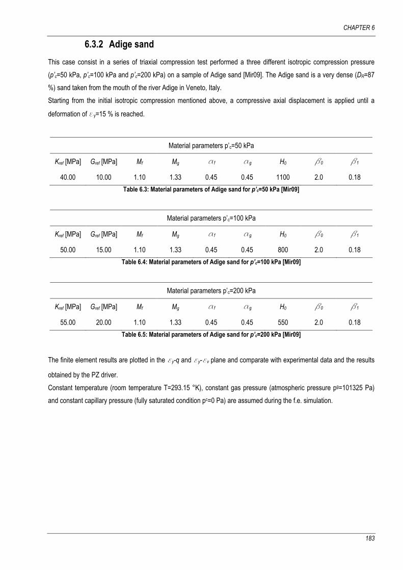
CHAPTER 6
183
6.3.2 Adige sand
This case consist in a series of triaxial compression test performed a three different isotropic compression pressure
(p’c=50 kPa, p’c=100 kPa and p’c=200 kPa) on a sample of Adige sand [Mir09]. The Adige sand is a very dense (DR=87
%) sand taken from the mouth of the river Adige in Veneto, Italy.
Starting from the initial isotropic compression mentioned above, a compressive axial displacement is applied until a
deformation of ey=15 % is reached.
Material parameters p’c=50 kPa
Kref [MPa] Gref [MPa] Mf Mg af ag H0 b0 b1
40.00 10.00 1.10 1.33 0.45 0.45 1100 2.0 0.18
Table 6.3: Material parameters of Adige sand for p’c=50 kPa [Mir09]
Material parameters p’c=100 kPa
Kref [MPa] Gref [MPa] Mf Mg af ag H0 b0 b1
50.00 15.00 1.10 1.33 0.45 0.45 800 2.0 0.18
Table 6.4: Material parameters of Adige sand for p’c=100 kPa [Mir09]
Material parameters p’c=200 kPa
Kref [MPa] Gref [MPa] Mf Mg af ag H0 b0 b1
55.00 20.00 1.10 1.33 0.45 0.45 550 2.0 0.18
Table 6.5: Material parameters of Adige sand for p’c=200 kPa [Mir09]
The finite element results are plotted in the ey-q and ey-ev plane and comparate with experimental data and the results
obtained by the PZ driver.
Constant temperature (room temperature T=293.15 °K), constant gas pressure (atmospheric pressure pg=101325 Pa)
and constant capillary pressure (fully saturated condition pc=0 Pa) are assumed during the f.e. simulation.

THE GENERALIZED PLASTICITY MODEL FOR WATER SATURATED SANDS
184
0
100
200
300
400
500
600
700
800
900
-16%-12%-8%-4%0%
Axial strain [-]
Dev
iato
ric
stre
ss [kP
a]
COMES-GEO
EXPERIMENTALDATA
p'c=50 kPa
p'c=200 kPa
p'c=100 kPa
Figure 6.12: Comparison between COMES-GEO and experimental results [Mir09] in eeeey-q plane
0
100
200
300
400
500
600
700
800
900
-16%-12%-8%-4%0%
Axial strain [-]
Dev
iato
ric
stre
ss [kP
a]
COMES-GEO
PZ driver
p'c=50 kPa
p'c=200 kPa
p'c=100 kPa
Figure 6.13: Comparison between COMES-GEO and PZ driver in eeeey-q plane

CHAPTER 6
185
-7%
-6%
-5%
-4%
-3%
-2%
-1%
0%
1%
-16%-12%-8%-4%0%
Axial strain [-]
Volu
met
ric
stra
in [-]
COMES-GEO
EXPERIMENTALDATA
p'c=50 kPa
p'c=200 kPa
p'c=100 kPa
Figure 6.14: Comparison between COMES-GEO and experimental results [Mir09] in eeeey-eeeev plane
-7%
-6%
-5%
-4%
-3%
-2%
-1%
0%
1%
-16%-12%-8%-4%0%
Axial strain [-]
Volu
met
ric
stra
in [-]
COMES-GEO
PZ driver
p'c=50 kPa
p'c=200 kPa
p'c=100 kPa
Figure 6.15: Comparison between COMES-GEO and PZ driver in eeeey-eeeev plane

THE GENERALIZED PLASTICITY MODEL FOR WATER SATURATED SANDS
186
0
100
200
300
400
500
600
700
800
900
-16%-12%-8%-4%0%
Axial strain [-]
Dev
iato
ric
stre
ss [kP
a]
COMES-GEO
EXPERIMENTAL
PZ driver
p'c=50 kPa
p'c=200 kPa
p'c=100 kPa
Figure 6.16: Comparison between COMES-GEO, experimental results [Mir09] and PZ driver in eeeey-q plane
-7%
-6%
-5%
-4%
-3%
-2%
-1%
0%
1%
-16%-12%-8%-4%0%
Axial strain [-]
Volu
met
ric
stra
in [-]
COMES-GEO
EXPERIMENTAL
PZ driver
p'c=50 kPa
p'c=200 kPa
p'c=100 kPa
Figure 6.17: Comparison between COMES-GEO, experimental results [Mir09] and PZ driver in eeeey-eeeev plane

CHAPTER 6
187
6.3.3 Dense sand
This case consist in a triaxial compression test performed with COMES-GEO and PZ driver for a dense sand [Ton03].
In fact, from Table 6.6, the value of Mf and Mg are Mf=0.95 and Mg=1.41 and then
% 4.6710041.195.0 ===
g
fR M
MD [6.91]
The isotropic compression pressure is p’c=124 kPa, and the loading path is compressive axial displacement applied until
a deformation of ey=15 % is reached.
Material parameters p’c=50 kPa
Kref [MPa] Gref [MPa] Mf Mg af ag H0 b0 b1
20.71 19.00 0.95 1.41 0.45 0.45 1000 2.2 0.12
Table 6.6: Material parameters of dense sand
The finite element results are plotted in the ey-q plane and comparate with the results obtained by the PZ driver.
Constant temperature (room temperature T=293.15 °K), constant gas pressure (atmospheric pressure pg=101325 Pa)
and constant capillary pressure (fully saturated condition pc=0 Pa) are assumed during the f.e. simulation.
100
150
200
250
300
350
400
-15%-13%-10%-8%-5%-3%0%
Volumetric strain [-]
Dev
iato
ric
stre
ss [kP
a]
COMES-GEO
PZ driver
Figure 6.18: Comparison between COMES-GEO and PZ driver in eeeey-q plane

THE GENERALIZED PLASTICITY MODEL FOR WATER SATURATED SANDS
188
References
[Cas69] Castro, G. (1969). Liquefaction of sands. Ph.D. thesis, Harvard Soil Mechanics Series No. 81, Harvard
University, Cambridge, Massachussets.
[Dru56] D.C. Drucker, 1956. On uniqueness in theory of plasticity. Quart. Appl. Match. 14, pp. 35–42.
[Dru59] D.C. Drucker, 1959. A definition of stable inelastic material. J. Appl. Mech. 26, pp. 101–106.
[Fro83] E. Frossard, Une équation d'éoulement simple pour les matériaux granulaires, Géotechnique, 33, 21-29,
1983.
[L&N87] Lade PV, Nelson RB. Modelling the elastic behaviour of granular materials. International Journal for
Numerical and Analytical Methods in Geomechanics 1987; 11:521–542.
[L&S67] Lee K.L. e H.B. Seed (1967) Drained strength characteristics of sands ASCE J. Geotech. Engrg. Vol.93
No.6, 117-141
[Lor85] Loret. The choice of elastic parameters for sand. International Journal for Numerical and Analytical Methods
in Geomechanics 1985; 9(3):285–292.
[M&Z84] Mroz. Z. and Zienkiewicz. O. C. (1984) Uniform formulation of constitutive equations for clays and sands.
Mechanics of Engineering Materials. C. S. Desai and R. H. Gallagher (eds). Wiley, Chichester. Ch. 22, pp.
415-449.
[Mir09] P. Mira, L. Tonni, M. Pastor and J. A. Fernandez Merodo. A generalized midpoint algorithm for the
integration of a generalized plasticity model for sands. International journal for numerical methods in
engineering. 2009; 77:1201–1223. DOI: 10.1002/nme.2445.
[Mol88] Molenkamp F. A simple model for isotropic non-linear elasticity of frictional materials. International Journal
for Numerical and Analytical Methods in Geomechanics 1988; 12:467–475.
[N&W79] Nova R, Wood DM. A constitutive model for sand in triaxial compression. International Journal for Numerical
and Analytical Methods in Geomechanics 1979; 3:255–278.
[P&Z86] Pastor, M. & Zienkiewicz, O.C. 1986. A generalized plasticity, hierarchical model for sand under monotonic
and cyclic loading. In G.N. Pande & W.F. Van Impe (eds), Proc. 2nd Int. Symp. on Numerical Models in
Geomechanics, Ghent, Belgium: 131–150. M. Jackson and Son Pub.
[Pas85] Pastor M, Zienkiewicz OC, Leung KH. Simple model for transient soil loading in earthquake analysis. II:
Non-associative models for sands. International Journal for Numerical and Analytical Methods in
Geomechanics 1985; 9:477–498.
[Pas90] Pastor, M., Zienkiewicz, O.C. & Chan, A.H.C. 1990. Generalized plasticity and the modelling of soil
behaviour. Int. J. Numer. and Anal. Methods in Geomechanics 14: 151–190.
[Ton03] Tonni, L., Gottardi, G., Cola, S., Simonini, P., Pastor, M. & Mira, P. (2003). Use of Generalized Plasticity to
describe the behaviour of a wide class of non-active natural soils. Proc. 3rd International Symposium on
Deformation Characteristics of Geomaterials, Lyon, 22 – 24 September 2003, Di Benedetto, H., Doanh, T.,
Geoffroy, H. & Sauzéat, C. (eds), pp. 1145-1153. Balkema Publishers, The Netherlands.
[Wil77] Wilde P. 1977 Two invariants dependent model of granular media, Arch. of Mechanics, 29, 799–809.

CHAPTER 6
189
[Z&M84] Zienkiewicz. O. C. and Mroz. Z. (1984) Generalized plasticity formulation and applications to geomechanics.
Mechanics of Engineering Materials. C. S. Desai and R. H. Gallagher (eds). Wiley, Chichester. Ch. 33, pp.
655-679.
[Z&P77] O.C. Zienkiewicz and G.N. Pande, Some useful forms of isotropic yield surfaces for soil and rock
mechanics. In: G. Godehus Editor, Finite elements in gemechanics Wiley, New York (1977), pp. 179–190.
[Zie85] Zienkiewicz OC, Leung KH, Pastor M. A simple model for transient soil loading in earthquake analysis.
International Journal for Numerical and Analytical Methods in Geomechanics 1985; 9:953–976.
[Zyt78] Zytynski M, Randolph MF, Nova R, Wroth CP. On modelling the unloading–reloading behaviour of soils.
International Journal for Numerical and Analytical Methods in Geomechanics 1978; 2:87–94.


CHAPTER 7
191
7 THE GENERALIZED PLASTICITY MODEL FOR
UNSATURATED SANDS
7.1 INTRODUCTION
Starting from the Pastor-Zienkiewicz model [Pas90] developed within the generalized plasticity theory for water saturated
soils, Bolzon et al. [Bol96] have proposed a model taking into account the conditions in partially saturated (Sw<1). This
new model is call here as BSZ model, results to be an extension of PZ model for partially saturated materials.
Since it was impossible to reproduce the behaviour of a soil in partially saturation only with the introduction of the
Bishop’s stress (see 2.6.1) in PZ model because the increase of soil compressibility with suction is not reproduced, the
largest amount of volumetric collapse appear always for fully saturated conditions for varying net mean stress, and the
isotropic yield limit decreases with increasing suction and this is in contrast with experimental observations, the authors
of [Bol96], proposed the BSZ model where a proper enhancement of the hierarchical PZ model allows to overcome
these drawbacks and that experimentally observed behaviour can be reproduced.
Hence the BSZ model gives advantages in partially saturated problems and where there is a transition from saturated to
unsaturated conditions. This is in particular the case when modelling dynamic behaviour of fully saturated and partially
saturated zones, as for instance in embankments, earth dams and slopes.
In literature other mathematical models were presented as for instance the one proposed by Wheeler and Sivakumar
[W&S95] where the BBM (Basic Barcelona Model) was improved, the bitensorial elastoplastic model HiSS-d1-unsat
proposed by Geiser [Gei99] or the model proposed by Jommi and Di Prisco [J&D94] where the degree of saturation was
introduce as second independent state variable in the hardening rule, and the ACMEG-S model [Fra08], which can be
derived by the already presented in chapter 5.
A further development of the BSZ model to non isothermal conditions has been proposed by Bolzon and Schrefler (BS
model) [B&S05] and will be presented at the end of this chapter.
Both these models have been implemented in COMES-GEO but only the implementation of the BSZ model has been
validated because of lack of material parameters for the non isothermal BS model.
For these reasons, the BSZ model can be considered validated although other tests was searching for a next future work
for have further evidence of predictive ability of the model, and the same is in progress for the BS model.

THE GENERALIZED PLASTICITY MODEL FOR UNSATURATED SANDS
192
7.2 BSZ MODEL
From section 6.2.1, and from Figure 6.4, we can write for a fully saturated soil
ppd
vdd e
vv ′′
==0
κεε [7.1]
in case of elastic loading and
ppd
vddd p
vevv ′
′=+=
0
λεεε [7.2]
In case of plastic loading, where
0
0
0
0
1 eee
vvv
v +−=−=ε [7.3]
ppd
Hd p
v ′′
=0
1ε [7.4]
Substitution of Bishop's definition [2.157] for partially saturated soil in terms of mean stress p'
sSpp wnet +=′ [7.5]
where gnet ppp −=
and s is the suction
in [7.1], [7.2] and [7.4], it would introduce a dependence of water content on volumetric strains.
Under monotonic loading, equation [7.4], can be integrated to give:
00
ln1
pp
Hpv ′
′=ε [7.6]
and if a rigid plastic behaviour is assumed (evp=ev)
00
00 ln
pp
Hv
vv′′
−= [7.7]
Introducing the Bishop’s stress [7.5] in [7.6] and [7.7] we obtain
sSpsSp
H wnet
wnetpv +
+=,00
ln1
ε [7.8]
sSpsSp
Hv
vvwnet
wnet
++−=
,00
00 ln [7.9]
As far as suction is kept constant, equations [7.6], [7.7], [7.8] and [7.9] give relationships between pressure and volume
changes which are similar to those of saturated soils, in accordance with experimental results (for instance [Kar86]) but it
is clear that the generally observed increase of soil compressibility with suction (for instance [Jos88]) is not taken into
account.
The yield function [6.63] begin now
( )
+−+−=c
wnetwnetf p
sSpsSpMqf
2
2 [7.10]
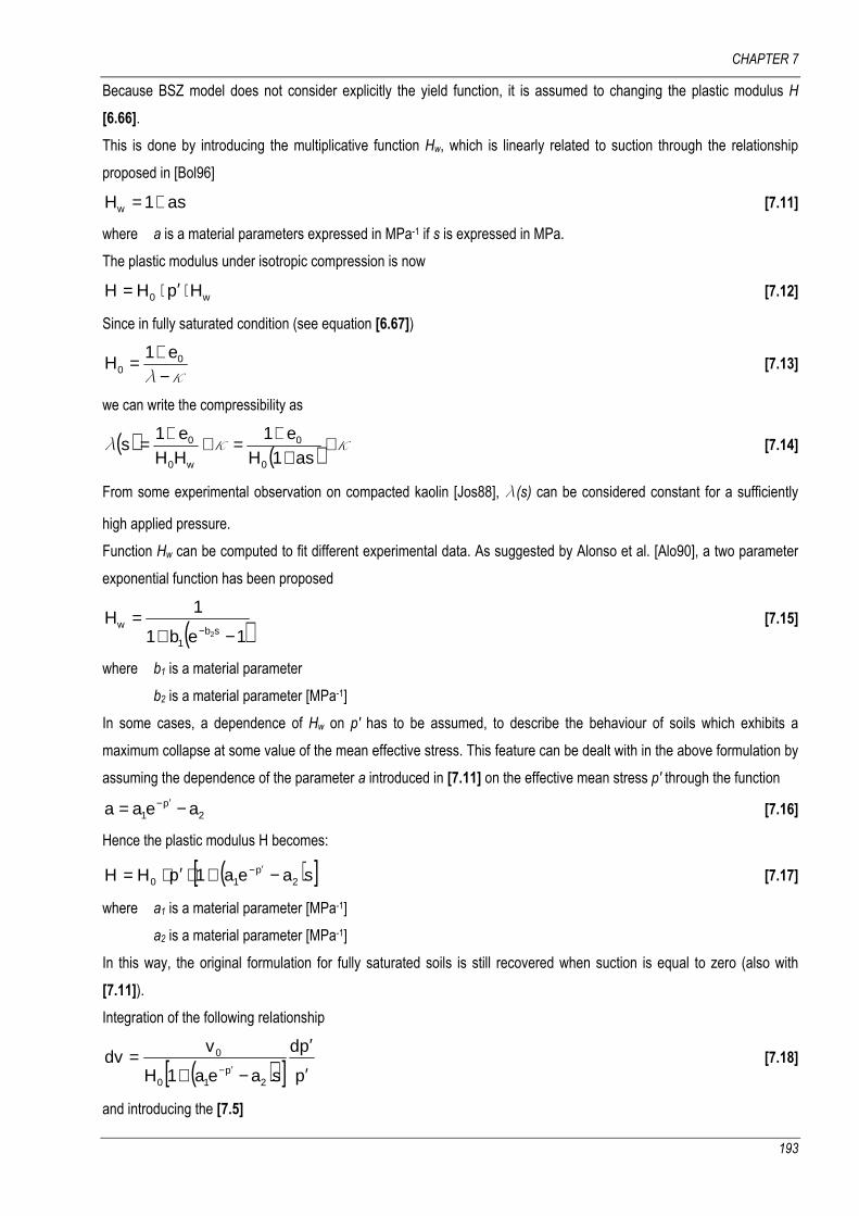
CHAPTER 7
193
Because BSZ model does not consider explicitly the yield function, it is assumed to changing the plastic modulus H
[6.66].
This is done by introducing the multiplicative function Hw, which is linearly related to suction through the relationship
proposed in [Bol96]
asHw += 1 [7.11]
where a is a material parameters expressed in MPa-1 if s is expressed in MPa.
The plastic modulus under isotropic compression is now
wHpHH ⋅′⋅= 0 [7.12]
Since in fully saturated condition (see equation [6.67])
κλ−+= 0
0
1 eH [7.13]
we can write the compressibility as
( ) ( ) κκλ ++
+=++=asH
eHHe
sw 1
11
0
0
0
0 [7.14]
From some experimental observation on compacted kaolin [Jos88], l(s) can be considered constant for a sufficiently
high applied pressure.
Function Hw can be computed to fit different experimental data. As suggested by Alonso et al. [Alo90], a two parameter
exponential function has been proposed
( )11
12
1 −+=
− sbw
ebH [7.15]
where b1 is a material parameter
b2 is a material parameter [MPa-1]
In some cases, a dependence of Hw on p' has to be assumed, to describe the behaviour of soils which exhibits a
maximum collapse at some value of the mean effective stress. This feature can be dealt with in the above formulation by
assuming the dependence of the parameter a introduced in [7.11] on the effective mean stress p' through the function
21 aeaa p −= ′− [7.16]
Hence the plastic modulus H becomes:
( )[ ]saeapHH p210 1 −+⋅′⋅= ′− [7.17]
where a1 is a material parameter [MPa-1]
a2 is a material parameter [MPa-1]
In this way, the original formulation for fully saturated soils is still recovered when suction is equal to zero (also with
[7.11]).
Integration of the following relationship
( )[ ] p
pd
saeaH
vdv
p ′
′
−+=
′−210
0
1 [7.18]
and introducing the [7.5]

THE GENERALIZED PLASTICITY MODEL FOR UNSATURATED SANDS
194
it can been shown that the maximum collapse is obtained at
2
1lnaa
pMAXv
=′∆
[7.19]
The ratio between the material constants a1, and a2 hence gives the critical value of the effective mean stress, at which
the maximum collapse is detected. On the other hand, the total amount of the collapse depends on the absolute value of
these parameters. The choice of assuming the material function a [7.11] a polynomial of p', would lead to undesired
singularities of the material behaviour, and has then been discarded.
Further refinements of the function Hw will require the determination of new material parameters, which may be
troublesome. This is out of the main purpose of the authors of BSZ model [Bol96], which is to give a simple and handily,
although reliable model of the behaviour of partially saturated soils.
As far as yield limits are concerned, a dependence of the hardening parameter pc on suction must be hypothized to find
correspondence between simulations and experimental observations. Once experiments give the initial yield limit p'y0 for
saturated condition, and value of p'y(s) at different suction values, a linear regression of data may often be considered
satisfactory
( ) ispsp y +′=′ 0 [7.20]
whence
( )sSipp wynety −+′= 0, [7.21]
Since Sw<1, the condition i>1 is sufficient (not necessary) for py,net(s) to be an increasing function of suction.
The evolution of the yield surface during the plastic process will be then governed by the development of plastic strains.
Due to this assumption, one could introduce the reference value p'c of Bishop's pressure, characterizing the limit
situation where no plastic strains develop as a consequence of suction changes. Then it must result that
( )c
y
wc
ypv p
sp
HHp
p
H ′′
=′′
= ln1
ln1
0
0
0
ε [7.22]
As a consequence, the evolution of the yield surface will be governed by the following relationship:
( ) ( ) κλ
κλ
−−
′′
=
′′
=′
′ s
c
y
H
c
y
c
y
p
p
p
p
p
sp w0
00 [7.23]
7.3 BS MODEL
This model [B&S05], has been developed from the BSZ model with the aim to model the behaviour of soils under
temperature changes. In particular, functions describing the yield surface and the compressibility modulus are modified
to account for the shrinking of the elastic domain and for the increase of irreversible volumetric strain with heating.
The behaviour of soils in non isothermal conditions was already describes in Chapters 4 and 5. Here we would like to
remark only a controversial aspect related to the effect of temperature upon compressibility with respect to loading.
According to most experimental observations, compressibility is slightly affected by temperature changes, especially in
fully saturated or nearly saturated conditions (see references [C&M68], [C&L04], [Sul02], [M&L97], [S&J90], [Sai91],
[Bur00] and [Del00]).
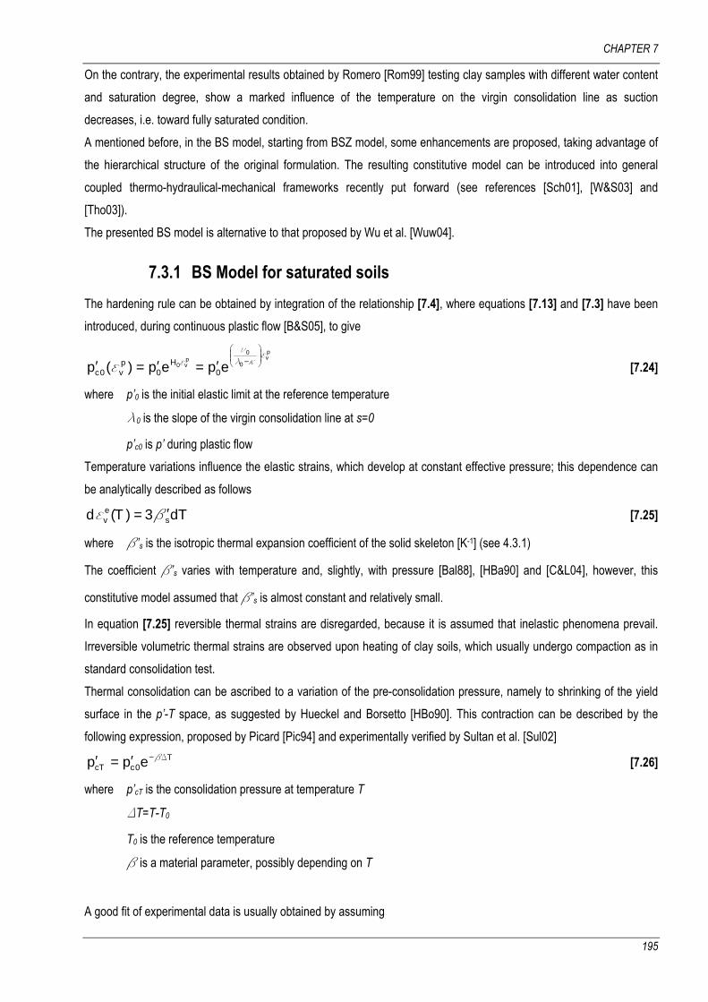
CHAPTER 7
195
On the contrary, the experimental results obtained by Romero [Rom99] testing clay samples with different water content
and saturation degree, show a marked influence of the temperature on the virgin consolidation line as suction
decreases, i.e. toward fully saturated condition.
A mentioned before, in the BS model, starting from BSZ model, some enhancements are proposed, taking advantage of
the hierarchical structure of the original formulation. The resulting constitutive model can be introduced into general
coupled thermo-hydraulical-mechanical frameworks recently put forward (see references [Sch01], [W&S03] and
[Tho03]).
The presented BS model is alternative to that proposed by Wu et al. [Wuw04].
7.3.1 BS Model for saturated soils
The hardening rule can be obtained by integration of the relationship [7.4], where equations [7.13] and [7.3] have been
introduced, during continuous plastic flow [B&S05], to give
pvp
v epepp Hpvc
εκλ
ν
εε
−′=′=′ 0
0
0000 )( [7.24]
where p’0 is the initial elastic limit at the reference temperature
l0 is the slope of the virgin consolidation line at s=0
p’c0 is p’ during plastic flow
Temperature variations influence the elastic strains, which develop at constant effective pressure; this dependence can
be analytically described as follows
dTTd sev βε ′= 3)( [7.25]
where b’s is the isotropic thermal expansion coefficient of the solid skeleton [K-1] (see 4.3.1)
The coefficient b’s varies with temperature and, slightly, with pressure [Bal88], [HBa90] and [C&L04], however, this
constitutive model assumed that b’s is almost constant and relatively small.
In equation [7.25] reversible thermal strains are disregarded, because it is assumed that inelastic phenomena prevail.
Irreversible volumetric thermal strains are observed upon heating of clay soils, which usually undergo compaction as in
standard consolidation test.
Thermal consolidation can be ascribed to a variation of the pre-consolidation pressure, namely to shrinking of the yield
surface in the p’-T space, as suggested by Hueckel and Borsetto [HBo90]. This contraction can be described by the
following expression, proposed by Picard [Pic94] and experimentally verified by Sultan et al. [Sul02]
TccT epp ∆β−′=′ 0 [7.26]
where p’cT is the consolidation pressure at temperature T
DT=T-T0
T0 is the reference temperature
b is a material parameter, possibly depending on T
A good fit of experimental data is usually obtained by assuming

THE GENERALIZED PLASTICITY MODEL FOR UNSATURATED SANDS
196
0
0
0 31
3 He pp αακλ
β =−
+= [7.27]
where ap is a positive scalar (function) [K-1]
so that 3apDT represents the equivalent unrecoverable volumetric strain.
Relationship [7.27] is equivalent to that proposed by Modaressi and Laloui [M&L97] when
TT
p
bTa +=
∆
13α [7.28]
A different analytical expression has been considered by Cekerevac and Laloui [C&L04], but the essential features of the
above-modelled material response to heating are maintained unaltered (see chapter 4).
Combination of [7.24], [7.26] and [7.27] returns
)3(0
0),( THpvcT
ppvepTp ∆∆ αεε −′=′ [7.29]
The influence of temperature on both elastic and post-yield compressibility parameters (k and l0, and henceforth H0) is
somewhat controversial, but in most materials in saturated or nearly saturated condition, consolidation curves remain
substantially parallel at different temperature (see references [C&M68], [Rob96], [HBa90], [C&L04], [Sul02], [M&L97] and
[Bur00]).
The capability of this model to reproduce the peculiar features of fully saturated soil behaviour under temperature
changes is visualized in [B&S05].
Some clays tested in oedometric conditions at nearly saturated states [Rom99], show a peculiar behaviour characterized
by an increase of both the compression modulus l and the amount of irreversible volumetric strain with temperature,
which develops for a given effective pressure change under isothermal conditions.
These correlated effects are easily accounted for in the present model, by introducing a suitable dependence of the
hardening modulus H0 on temperature, as proposed in [B&S05]
ThhTH
T∆+=
00
1)( [7.30]
Relationship [7.30] returns the simplest approximation for lo(T) which thus increases linearly with temperature.
The evolution of the yield surface, and its consequences on the amount of irreversible collapse developed by a material
sample loaded at different temperature, are shown in [B&S05].
7.3.2 BS Model for partially saturated soils
Available experimental results show that the behaviour of partially saturated soils is substantially similar at room and at
high temperature. Main differences may concern the amount of irreversible volumetric strain which develops upon
wetting. Shrinkage upon drying is also enhanced at high temperature [Rom03] but this aspect is not included in the BS
model.
Following some results published by Saix and Jouanna [S&J90], Saix [Sai91], Recordon [Rec93] and Romero [Rom99]
[Rom03], the authors of [B&S05] have outlined the following main features of the thermal behaviour of partially saturated
soils on which base the developed model:

CHAPTER 7
197
1. water content at higher temperature is smaller than at reference (ambient) temperature, but the shape of water
retention curve is almost insensitive to heating (differently from that proposed in ACMEG-TS);
2. suction versus saturation relationship is even less affected by temperature changes;
3. the amount of irreversible strains which develop during wetting may increase with temperature for those soils
which exhibit, as peculiar features, irreversible swelling with suction decrease (even at reference temperature)
and thermal dependence of the hardening moduli.
The water content and the saturation degree of soils were described in 5.3.
As seen for the family of ACMEG models, partially saturated soils develop unrecoverable volumetric strains with heating
in normally consolidated conditions, while thermal strains are mainly reversible in overconsolidated states, exactly as in
the case of full saturation. The amount of thermal deformation can be quantified by the relationships [7.4], [7.25], [7.26]
and [7.27].
As already observed for BSZ model, in most instances preconsolidation stress reduces with heating, while temperature
changes do not affect significantly the elastic and plastic material compressibility. Therefore, yield surface can be
described as follows in the p’-s-T space
)(),(
),(sH
r
pvcT
rcsT
w
pTp
pTsp
′∆′′=∆′ ε
[7.31]
Writing the relation [7.11] in terms of l and k changing with s
( ) ( ) κλ
κλ
−−=
ssHw
0 [7.32]
and then introducing equations [7.32] and [7.29] into [7.31], the yield surface is obtained as
)3()(
)(0
00
),(T
ss
rrcsT
ppv
epp
pTsp∆
∆αε
κλ
νκλ
κλ
−−
−−
′′′=′ [7.33]
Equation [7.33] is validated in [B&S05].
A compaction process usually takes place during soil wetting. The corresponding unrecoverable strain can be evaluated
through relation
( ) ppd
sHHd
w
pv ′
′=
0
1ε [7.34]
being p’=p’csT, account taken of the fact that plastic compatibility implies the evolution of the consolidation stress with
suction changes. The amount of irreversible strain which develops upon wetting is substantially similar at room and high
temperature, consistently with the results of some available experimental investigation [Rom99] and [Rom03].
In the same references [Rom99] and [Rom03], is shown that by some soils irreversible swelling upon wetting occurs
even at reference temperature. Contemporarily both of the slopes of the virgin compression line and of the
unrecoverable volumetric strain increasing with temperature is observed during oedometric tests.
Irreversible swelling can be described by a proper choice of the hardening function; for instance, expression [7.16]
foresees volume increments corresponding to suction reduction for some pressure ranges and suitably chosen
parameters a1 and a2 [Bol96].

THE GENERALIZED PLASTICITY MODEL FOR UNSATURATED SANDS
198
The possible increase of irreversible strain with temperature during the soil wetting is instead easily accounted for even
by the simplest version of the present constitutive model, account taken of the contemporarily observed variation of the
compressibility modulus.
7.4 VALIDATION OF THE IMPLEMENTATION OF THE BSZ MODEL IN
THE F.E. CODE COMES-GEO
As mentioned in section 7.1, the validation of the implementation in the finite element code COME-GEO has been done
only for the BSZ model. BS model has been only implemented and the numerical implementation will be validated in the
near future.
For the numerical validation of the BSZ model, a series of triaxial compression test in saturated state served to calibrate
the model, and then, some predictive triaxial compression tests were made in unsaturated conditions. The tests were
taken from the extensive experimental investigation conduced by Geiser [Gei99] and [S&S05]. The soil used is a slime of
the Sion region in Switzerland composed by slime (72%), clay (8%) and sand (20%).
The tests performed by Geiser were made for different preconsolidation pressure. For validation of the BSZ model it was
considered the cases with p’c=600 kPa, p’c=400 kPa and p’c=100 kPa.
Material parameters (Geiser)
Eref [MPa] n Kref [MPa] Gref [MPa] ne pref [MPa] Mg0 n (porosity)
110.00 0.35 122.22 40.74 0.5 0.40 1.18 0.4286
Material parameters (calibrated)
Mf0 af ag H0 b0 b1 a [MPa-1]
1.18 0.45 0.45 235 1.70 0.25 5.00
Hydraulic parameters (modified Safai and Pinder)
Sirr b [cm-1] g r’
0.086 6.50 2.20 1.00
Table 7.1: Material parameters of Sion silt tested by Geiser
The material parameters were found through the calibration of the model with the triaxial tests at fully saturated state.
Therefore, before moving on to the analysis in partially saturation conditions, a comparison was made, with other triaxial
test with different p’c having the same parameters.
For the elastic modulus, Geiser suggest to use a relationship similar to [4.6] and [4.7]
en
refref p
pE=E
′′
[7.35]
where Eref=110 MPa

CHAPTER 7
199
ne=0.5
pref=0.4 MPa
Being n=0.35, Kref and Gref are computed according to [4.6] and [4.7].
The material parameters are shown in Table 7.1.
Temperature and gas pressure are constant at T=20 °C and pg=101325 Pa.
The water retention constitutive law chosen for this test is the one proposed from Safai and Pinder (see Figure 7.1)
where at three suctions (in add at the saturated case s=0 MPa) correspond the following degree of saturation
s=50 kPa Sw=0.930
s=100 kPa Sw=0.740
s=200 kPa Sw=0.410
s=0,
05 M
pa
s=0,
10 M
pa
s=0,
20 M
Pa
0,1
0,2
0,3
0,4
0,5
0,6
0,7
0,8
0,9
1,0
1,1
0,01 0,10 1,00
Suction [MPa]
Deg
ree
of sa
tura
tion [-]
Figure 7.1: Water retention constitutive law Safai and Pinder for Sion silt
In the next graphs (Figure 7.2 and Figure 7.3) are shown first the comparison between the experimental data [Gei99]
and the simulation of the triaxial compression test with a confining pressure p’c=600 kPa and in fully saturated state and
then the comparison with the tests performed with p’c=100 kPa and p’c=400 kPa.
The simulation referred to the Figure 7.2 served, as mentioned above, for the calibration of the model through the fitting
experimental data for the parameters that are properly only of the BSZ model.
In the Figure 7.3 instead the results was predicted and then compared with the experimental one.
Until this point, the BSZ model coincide with the PZ (because s=0).
At the same mode, the parameter a for the extension of the PZ model to BSZ model is obtained with a calibration for the
triaxial compression at s=0.10 MPa for the two confining pressure p’c=400 kPa and p’c=600 kPa.

THE GENERALIZED PLASTICITY MODEL FOR UNSATURATED SANDS
200
The simulation with the predicted results are the two triaxial tests at p’c=600 kPa at two different suction s=0.05 MPa and
s=0.20 Mpa.
0
250
500
750
1000
1250
1500
-20%-15%-10%-5%0%
Axial strain [-]
Dev
iato
ric
stre
ss [kP
a]
COMES-GEO
EXPERIMENTAL
p'c=600 kPa
s=0,00 MPa
Figure 7.2: Triaxial test for the calibration of the model p’c=600 kPa and s=0.00 MPa
0
250
500
750
1000
-20%-15%-10%-5%0%
Axial strain
Dev
iato
ric
stre
ss [kP
a]
COMES-GEO
EXPERIMENTAL
p'c=400 kPa
s=0,00 MPa
p'c=100 kPa
s=0,00 MPa
Figure 7.3: Comparison between experimental data [Gei99] and BSZ model in COMES-GEO after calibration of material
parameter (Figure 7.2) p’c=100 kPa and p’c=400 kPa and s=0.00 MPa

CHAPTER 7
201
0
250
500
750
1000
-20%-15%-10%-5%0%
Axial strain [-]
Dev
iato
ric
stre
ss [kP
a]
COMES-GEO
EXPERIMENTAL
p'c=400 kPa
s=0,10 MPa
Figure 7.4: Triaxial test for the calibration of the parameter a p’c=400 kPa and s=0.10 MPa
0
250
500
750
1000
1250
1500
-20%-15%-10%-5%0%
Axial strain [-]
Dev
iato
ric
stre
ss [kP
a]
COMES-GEO
EXPERIMENTAL
p'c=600 kPa
s=0,10 MPa
Figure 7.5: Triaxial test for the calibration of the parameter a p’c=600 kPa and s=0.10 MPa

THE GENERALIZED PLASTICITY MODEL FOR UNSATURATED SANDS
202
0
250
500
750
1000
1250
1500
-20%-15%-10%-5%0%
Axial strain [-]
Dev
iato
ric
stre
ss [kP
a]
COMES-GEO
EXPERIMENTAL
p'c=600 kPa
s=0,05 MPa
Figure 7.6: Comparison between experimental data [Gei99] and BSZ model in COMES-GEO after calibration of material
parameter a p’c=600 kPa and s=0.05 MPa
0
250
500
750
1000
1250
1500
-20%-15%-10%-5%0%
Axial strain [-]
Dev
iato
ric
stre
ss [kP
a]
COMES-GEO
EXPERIMENTAL
p'c=600 kPa
s=0,20 MPa
Figure 7.7: Comparison between experimental data [Gei99] and BSZ model in COMES-GEO after calibration of material
parameter a p’c=600 kPa and s=0.20 MPa

CHAPTER 7
203
7.5 REMARKS
1. Numerical validation of the BSZ and BS models need of further investigations once the complete set of material
parameters of these models could be determined or identified.
2. An enhanced BSZ constitutive model was developed by Santagiuliana and Schrefler [S&S06] based on the
constitutive model proposed by Jommi and Di Prisco [J&D94] for partially saturated soils.
3. A future development of this Phd thesis will be the implementation of the eBSZ (enhanced Bolzon-Schrefler-
Zienkiewicz constitutive model).

THE GENERALIZED PLASTICITY MODEL FOR UNSATURATED SANDS
204
References
[Alo90] Alonso EE, Gens A, Josa A. A constitutive model for partially saturated soils. Géotechnique 1990; 40:405–
430.
[B&S05] Bolzon G. and Schrefler B.A. (2005). Thermal effects in partially saturated soils: a constitutive model.
International Journal for Numerical and Analytical Methods in Geomechanics, 29(9): 861-877.
[Bal88] Baldi G, Hueckel T, Pellegrini R. Thermal volume changes of mineral-water system in low porosity clay
soils. Canadian Geotechnical Journal 1988; 25:807–825.
[Bol96] Bolzon G, Schrefler BA, Zienkiewicz OC. Elastoplastic soil constitutive law generalized to partially saturated
states. Géotechnique 1996; 46:279–289.
[Bur00] Burghignoli A, Desideri A, Miliziano S. A laboratory study on the thermomechanical behaviour of clayey
soils. Canadian Geotechnical Journal 2000; 37:764–780.
[C&L04] Cekerevac C. and Laloui L. (2004). Experimental study of thermal effects on the mechanical behaviour of a
clay. International Journal for Numerical and Analytical Methods in Geomechanics, 28(3): 209-228.
[C&M68] Campanella R.G. and Mitchell J.K. (1968). Influence of temperature variations on soil behaviour. Journal of
the Soil Mechanics and Foundation Division, ASCE, 94: 709-734.
[Del00] Delage P, Cui YJ, Sultan N. On the thermal consolidation of Boom clay. Canadian Geotechnical Journal
2000; 37:343–354.
[Fra08] François B. (2008). Thermo-Plasticity of Fine-Grained Soils at Various Saturation States: Application to
Nuclear Waste Disposal. PhD Thesis. École Polytechnique Fédérale De Lausanne. Suisse.
[Gei99] Geiser F. (1999). Comportement mécanique d'un limon non saturé: Etude expérimentale et modélisation
constitutive. PhD Thesis, EPFL, Lausanne, Switzerland.
[HBa90] Hueckel T, Baldi G. Thermo-plasticity of saturated clays: experimental constitutive study. ASCE Journal of
Geotechnical Engineering 1990; 116(12):1778–1796.
[HBo90] Huechel T, Borsetto M. Thermo-plasticity of saturated soils and shales: Constitutive equations. ASCE
Journal of Geotechnical Engineering 1990; 116(12):1765–1776.
[J&D94] Jommi C., di Prisco C. (1994). Un semplice approccio teorico per la modellazione del comportamento
meccanico di terreni granulari parzialmente saturi. Il ruolo dei fluidi nei problemi di ingegneria geotecnica,
Mondovì, Vol.1, II: 167,188.
[Jos88] Josa, A. (1988). Un modelo eslastoplirstico para suelos no saturados. Tesis Doctoral. Universitat
Politecnica de Catalunya, Barcelona.
[Kar86] Karube, D. (1986). New concept of effective stress in unsaturated soil and its proving tests. ASTM Symp. on
Advanced Triaxial Testing of Soil and Rock, ST 977,539-552. Philadelphia: American Society for Testing
and Materials.
[M&L97] Modaressi H. and Laloui L. (1997). A thermo-viscoplastic constitutive model for clays. International Journal
for Numerical and Analytical Methods in Geomechanics, 21(5): 313–315.
[Pas90] Pastor, M., Zienkiewicz, O.C. & Chan, A.H.C. 1990. Generalized plasticity and the modelling of soil
behaviour. Int. J. Numer. and Anal. Methods in Geomechanics 14: 151–190.

CHAPTER 7
205
[Pic94] Picard J. Ecrouissage thermique des argiles saturées: application au stockage des déchets radioactifs.
Doctoral Thesis. Ecole Nationale de Ponts ae Chaussées, 1994.
[Rec93] Recordon E. Déformabilité des sols non saturés a diverses températures. Revue Francoise de
Géotechnique 1993; 65:37–56.
[Rob96] Robinet J-C, Rahbaoui A, Plas F, Lebon P. A constitutive thermomechanical model for saturated clays.
Engineering Geology 1996; 41:145–169.
[Rom03] Romero E, Gens A, Lloret A. Suction effects on a compacted clay under non-isothermal conditions.
Géotechnique 2003; 53(1):65–81.
[Rom99] Romero E. (1999). Characterisation and thermo-mechanical behaviour of unsaturated Boom clay: An
experimental study. PhD Thesis, UPC, Barcelona.
[S&J90] Saix C, Jouanna P. Appareil triaxial pour l’étude du comportement thermique de sols non saturés. Canadian
Geotechnical Journal 1990; 27:119–128.
[S&S06] Santagiuliana R., Schrefler B.A. :2006, Enhancing The Bolzon-Schrefler-Zienkiewicz Constitutive Model For
Partially Saturated Soil, Transport in porous media, 65:1-30.
[Sai91] Saix C. Consolidation thermique par chaleur d’un sol non saturé. Canadian Geotechnical Journal 1991;
28:42–50.
[Sch01] B.A. Schrefler. Environmental Geomechanics. CISM Courses and Lectures No 417, Springer Verlag Wien,
New York, 2001.
[Sul02] Sultan N, Delage P, Cui YJ. Temperature effects on the volume change behaviour of Boom clay.
Engineering Geology 2002; 64:135–145.
[Tho03] Thomas HR, Yang HT, He Y, Cleall PJ. A multi-level parallelized substructuring-frontal solution for coupled
thermo/hydro/mechanical problems in unsaturated soils. International Journal for Numerical and Analytical
Methods in Geomechanics 2003; 27:951–976.
[W&S03] Wang Z, Schrefler BA. Fully coupled thermo-hydro-mechanical analysis by an algebraic multigrid method.
Engineering Computations 2003; 20:211–229.
[W&S95] Wheeler, S.J. & Sivakumar, V. (1995). An elasto-plastic critical state framework for unsaturated soil.
Géotechnique, 45, No. 1, 35-53.
[Wuw04] Wu W, Li X, Charlier R, Collin E. A thermo-hydro-mechanical constitutive model and its numerical modelling
for unsaturated soils. Computers and Geotechnics 2004; 31:155–167.


CHAPTER 8
207
8 APPLICATION TO GEO-ENVIRONMENTAL ENGINEERING
PROBLEMS
As reported in the first chapter of this work, the implementation and the numerical validation of advanced constitutive
models for soils, is needed to study the complex THM nature of several geo-environmental engineering problems. In this
chapter two works in progress are shown: the simulation of the long-term behaviour of a deep nuclear waste disposal
and of land subsidence due to gas production. Both the cases are complex and it is difficult to completely define their
study because of the multitude of uncertainties and variables. For each case, it will be shown a description of the
problem, the finite element discretization with the boundary conditions and, the most significant preliminary results.
Furthermore, future developments will be suggested.
8.1 DEEP NUCLEAR WASTE DISPOSAL
8.1.1 Introduction
This work is the results of collaboration with the research group of Prof. L. Laloui.
The exercise proposed from the Agence nationale pour la gestion des déchets radioactifs [BRGM91] has been simulated
with the aim to analyze the THM interaction of a theoretical storage system for radioactive waste of and many steps of
type B and C (i.e. intermediate and high level waste). The results described in the following summarize those reported in
[Lui06], [Pas08], [Pas09] and [San10].
The storage system consists of three horizontal tunnels 80 distant with a vertical section 6 m high and 5 m large. In each
tunnel, a series of vertical wells are drilled with a diameter of 50 cm and an high of 55 m (of which 40 m are filled with the
radioactive waste and the last 5 to form a clay stopper).
Two wheelbases between the wells, 10 m or 20 m, and two depths of the tunnels, 400 m or 750 m, have been analyzed.
In particular the following analyses have been performed:
1. Case 1-A: tunnels’ dept of 400 m and wells’ wheelbase of 20 m
2. Case 1-B: tunnels’ dept of 400 m and wells’ wheelbase of 10 m
3. Case 2-A: tunnels’ dept of 750 m and wells’ wheelbase of 20 m
4. Case 2-B: tunnels’ dept of 750 m and wells’ wheelbase of 10 m

APPLICATION TO GEO-ENVIRONMENTAL ENGINEERING PROBLEMS
208
Figure 8.1: Tunnels and wells scheme
8.1.2 Source of temperature
Here a nuclear waste of type C for a period of about 200 years starting from the storage
of the containers into the wells is considered. Each container has the same releases of
heat described from the power law depicted in Figure 8.3.
This release has been transformed in five equivalent heat sources applied in five
specific points at a constant distance of 12.5 m (see Figure 8.2) that are considered to
be direct in contact with the host rock. This temperature history increases, from 30 °C to
98 °C in the first 30 years and then a slowly decreases in the next 180 years (Figure
8.4).
Figure 8.2: Distribution of temperature source

CHAPTER 8
209
0
50
100
150
200
250
300
350
400
450
500
0 50 100 150 200 250
Time [year]
Pow
er [W
]
Figure 8.3: Power released on time from each container
293
303
313
323
333
343
353
363
373
0 30 60 90 120 150 180 210
Time [year]
Tem
per
ature
[K
]
Figure 8.4: Temperature released on time from each source

APPLICATION TO GEO-ENVIRONMENTAL ENGINEERING PROBLEMS
210
8.1.3 Material parameters
The material parameters are obtained from a series of triaxial compression tests made by the B.R.G.M. geotechnical
laboratory of Orleans on samples of clay of Montcornet [BRGM91] and are listed in Table 8.1and Table 8.2 for Case 1
and Case 2 respectively. The tests were performed in drained and undrained conditions, monotonic or cyclical load
conditions and with different confining pressure and load speed.
CASE 1
sample name sample deep
[m] confining
[MPa] gs [kg/m³] n k [m/s]
A 1950 437.7-438.0 5.30-10.60 2070 0.37 10-12
Elastic parameters
Kref [MPa] Gref [MPa] ne b’s [°C-1]
200.0 120.0 0.70 3.010-5
Isotropic plastic parameters
b c reiso p’c [MPa] gT
12.0 0.002 0.005 15.00 0.4
Deviatoric plastic parameters
b d Ø’0 [°] redev a g a
1.0 1.5 15 0.005 0.001 4.510-5 1.0
Table 8.1: Material parameters for Case 1
CASE 2
sample name sample deep
[m] confining
[MPa] gs [kg/m³] n k [m/s]
A 2149 779.7-780.0 12.00-19.80 2320 0.22 10-13
Elastic parameters
Kref [MPa] Gref [MPa] ne b’s [°C-1]
250.0 130.0 0.70 3.010-5
Isotropic plastic parameters
b c reiso p’c [MPa] gT
12.0 0.002 0.005 36.00 0.4
Deviatoric plastic parameters
b d Ø’0 [°] redev a g a
1.0 1.5 28 0.005 0.007 4.510-5 1.0
Table 8.2: Material parameters for Case 2

CHAPTER 8
211
Not all the parameters necessary for ACMEG-T model were found in the B.R.G.M. report [BRGM91], in particular for the
missing parameter those relative to Boom clay have been selected.
8.1.4 Initial and boundary conditions
The problem can be analyzed in plane strain conditions and hence two different bi-dimensional problems are solved: a
vertical section surrounding the central tunnel and containing a well (Figure 8.5) and an horizontal section containing
three wells (Figure 8.6). 20
8
804040
5315
5
3530
30
PLOT POINT
pg pw T
Initial condition
1017 982 964
927
582
290
Figure 8.5: Boundary and initial condition of vertical section
40 40
510
105
30
80
SOURCE POINTPLOT POINT
719834911 642 618634
Figure 8.6: Boundary conditions of horizontal section

APPLICATION TO GEO-ENVIRONMENTAL ENGINEERING PROBLEMS
212
The initial and boundary conditions are described now.
8.1.4.1 Gas pressure
Because the host rock is initially water saturated, the gas pressure is assumed constant and equal to the atmospheric
pressure patm=101325 Pa for all the nodes of the spatial discretization.
8.1.4.2 Capillary pressure
Similarly the water pressure presents the hydrostatic distribution. From the relation
( ) hhppppp wwatmgwgc γγ −=+−=−= [8.1]
where h is the deep from the top surface
it is possible to calculate the capillary pressure (negative) to be imposed on the boundaries.
8.1.4.3 Temperature
A temperature gradient of 30 K/100 m starting from the ambient temperature of 15 °C at the surface in contact with the
atmosphere has been assumed. Hence the following relationship has been used to compute the temperature distribution
on the lateral boundaries:
hTT amby ⋅+= 03.0 [8.2]
where h is the deep from the top (positive quantities)
Tamb=15 °C
For the two cases the initial conditions are the following
Case 1 Case 2
y0 [m] -400.00 -750.00
ysup [m] -350.00 -700.00
yinf [m] -550.00 -900.00
T0 [°C] 27.00 37.50
Tsup [°C] 25.00 36.00
Tinf [°C] 31.50 42.00
Table 8.3: Summary of initial condition of temperature
8.1.4.4 Displacement
For symmetry (see Figure 8.1) the boundary conditions for the horizontal displacement are those shown in Figure 8.5.
Vertical displacements are constrained on the bottom surface (see Figure 8.5).
At the top of the mesh a total vertical stress is applied to simulate the weight of 350 m of water saturated soil for Case 1
and 700 m for Case 2.

CHAPTER 8
213
For the calculation of the soil load the following relation was used
( )[ ] ghnnq wsy ⋅⋅+−= γγ 1 [8.3]
where gs [kg/m3] is the solid grain density
gw=1000 kg/m3 is the water density
n is the porosity
g=9.81 m/s2 is the gravity acceleration
h [m] is the high of soil from the surface in contact with the atmosphere.
For Case 1 we have from Table 8.1 that qy= 5’748’022,35 Pa (because gs=2070 kg/m3 and n=0.37).
For Case 2 we have from Table 8.2 that qy=13’937’263,20 Pa (because gs=2320 kg/m3 and n=0.22).
8.1.5 Mesh
The mesh for both the horizontal and vertical sections is composed by eight node quadrilateral elements, as shown in
Figure 8.5 and Figure 8.6.
The vertical section is discretized with 896 elements and 2836 nodes (14180 dof), while the horizontal one with 384
elements and 1241 nodes (6205 dof).
8.1.6 Simulations
As reported in the following Table 8.4, seven different analysis have been performed. The early three present different
peak value Tmax of the temperature law of Figure 8.4, see Figure 8.7.
In particular, the third case simulates a failure condition of the canisters.
N° simulations
Deep [m]
Well’s wheelbase [m]
Time analysis [Year]
Tmax
[K]
1 400 10 210 95
2 400 10 210 178
3 400 10 210 300
4 400 10 400 95
5 400 20 210 95
6 400 10 210 95
7 400 20 210 95
Table 8.4: Summary of simulations

APPLICATION TO GEO-ENVIRONMENTAL ENGINEERING PROBLEMS
214
293
343
393
443
493
543
593
0 30 60 90 120 150 180 210
Time [year]
Tem
per
ature
[K
]
Tmax=95°C
Tmax=178°C
Tmax=300°C
Figure 8.7: Temperature of simulations
8.1.7 Results
The finite element analysis is performed first by computing the initial mechanical conditions in equilibrium with the given
boundary conditions and the gravity load. To this end two different elastic analysis have been performed. The first one is
an analysis that considers the material as linear elastic while the second one considers the material as non-linear elastic.
Then the transient analysis is applied by considering the temperature loading function plotted in Figure 8.7.
In particular a comparison between the node 290, 582 and 927 (see Figure 8.5) of vertical section are shown for Case 1
(with dept 400 m) and Case 2 (with dept 750 m).
Then, the results of horizontal section are shown for nodes 618 and 634 (see Figure 8.6) for Case A (with wheelbase of
20 m) and Case B (with wheelbase of 10 m).
From the time histories plotted in Figure 8.8 to Figure 8.13 it could be concluded that the results in terms of T, ev and
evp is similar for the two selected tunnel depth. The only difference is in the initial temperature due to different initial and
boundary conditions. An opposite conclusion should be done when analyzing the effect of different wheelbase. The
deformation due to the thermal gradient is bigger in the case with wheelbase of 10 m (about twice).
However the amount of the deformation is negligible because the high confining pressure, and therefore both the
wheelbase can be adopted.

CHAPTER 8
215
295
305
315
325
335
345
355
0 40 80 120 160 200
Time [year]
Tem
per
ature
[K
]
400 m - Node 290
400 m - Node 582
400 m - Node 927
700 m - Node 290
700 m - Node 927
700 m - Node 927
Figure 8.8: Vertical section – Temperature T
-6,0E-05
-4,0E-05
-2,0E-05
0,0E+00
2,0E-05
4,0E-05
6,0E-05
8,0E-05
1,0E-04
1,2E-04
1,4E-04
0 40 80 120 160 200
Time [year]
Volu
met
ric
tota
l st
rain
[-]
400 m - Node 290
400 m - Node 582
400 m - Node 927
700 m - Node 290
700 m - Node 927
700 m - Node 927
Figure 8.9: Vertical section – Volumetric total strain eeeevT
-3,5E-05
-3,0E-05
-2,5E-05
-2,0E-05
-1,5E-05
-1,0E-05
-5,0E-06
0,0E+00
0 40 80 120 160 200
Time [year]
Volu
met
ric
pla
stic
str
ain [-]
400 m - Node 290
400 m - Node 582
400 m - Node 927
700 m - Node 290
700 m - Node 927
700 m - Node 927
Figure 8.10: Vertical section – Volumetric plastic strain eeeevp

APPLICATION TO GEO-ENVIRONMENTAL ENGINEERING PROBLEMS
216
300
310
320
330
340
350
360
0 40 80 120 160 200
Time [year]
Tem
per
ature
[K
]
10 m - Node 618
10 m - Node 634
20 m - Node 61820 m - Node 634
Figure 8.11: Horizontal section – Temperature T
-8,E-04
-7,E-04
-6,E-04
-5,E-04
-4,E-04
-3,E-04
-2,E-04
-1,E-04
0,E+00
1,E-04
2,E-04
0 40 80 120 160 200
Time [year]
Volu
met
ric
tota
l st
rain
[-]
10 m - Node 618
10 m - Node 634
20 m - Node 618
20 m - Node 634
Figure 8.12: Horizontal section – Volumetric total strain eeeevT
-3,0E-05
-2,5E-05
-2,0E-05
-1,5E-05
-1,0E-05
-5,0E-06
0,0E+00
0 40 80 120 160 200
Time [year]
Volu
met
ric
pla
stic
str
ain [-]
10 m - Node 618
10 m - Node 634
20 m - Node 618
20 m - Node 634
Figure 8.13: Horizontal section – Volumetric plastic strain eeeevp

CHAPTER 8
217
Now the contours of the volumetric total strain ev in the time are shown for the vertical section (Case 1: tunnels’ dept of
400 m).
Figure 8.14: t=2 years
Figure 8.15: t=7,5 years
Figure 8.16: t=15 years
Figure 8.17: t=22,5 years

APPLICATION TO GEO-ENVIRONMENTAL ENGINEERING PROBLEMS
218
Figure 8.18: t=30 years
Figure 8.19: t=45 years
Figure 8.20: t=145 years
Figure 8.21: t=200 years

CHAPTER 8
219
8.1.8 Failure conditions
As mentioned in 8.1.6 a nuclear accident due to the failure of the containers in a well is simulated by the temperature law
reaching the 300 °C. At this temperature the liquid water in the soil close the heat source starts to evaporate and causes
desaturation of the near host rock (Figure 8.22).
At the same time, a quite large volumetric plastic bulb surrounding the well is described, as depicted in Figure 8.22.
For this simulation, ACMEG-TS model should be used to model correctly the occurrence of the partially saturated
condition. This will be performed in the near future.
Figure 8.22: Volumetric plastic strain and Degree of saturation state for the reached temperature of 300 °C.

APPLICATION TO GEO-ENVIRONMENTAL ENGINEERING PROBLEMS
220
8.2 SUBSIDENCE DUE TO GAS PRODUCTION
8.2.1 Introduction
In this section the problem described by Zhang et al. [Zha01] has been simulated. A gas reservoir of the type
investigated in this section contains gaseous and liquid phases at the same time and within it pressure gradients are
possible. As a consequence, the pressure measurements usually performed cannot represent what happens in the
whole reservoir. Moreover the reservoirs are in hydraulic continuity with confining aquifers and aquitards. A complete
mathematical model to simulate the mechanical behaviour of such a multiphase system needs therefore a mass balance
equation for all present fluids together with momentum balance equations for fluids and the mixture. All these equations
are coupled owing to the interactions between the fluids and the solid.
In this case the constitutive law BSZ is used because the reservoir is in partially saturated conditions.
Part of the material parameters are taken from Papamichos and Schei: “Characterization of Adriatic soft weak sediments
for subsidence” [P&S98], the others are taken from the parameter identification of Simoni and Schrefler [S&S01] or
extrapolated as illustrated in section 8.2.2.
8.2.2 Identification of parameters
8.2.2.1 Parameter from test
Figure 8.23: Location of the Ravenna Terra gas field and wells (Redrawn from [Men08]). Into the red circle there is the
Angela reservoir from which Core 1305 comes.

CHAPTER 8
221
In the following table the parameters given from Papamichos and Schei for “Core 1305”, which is one of the tests
performed by the authors (Figure 8.23), are reported. This is a laboratory experiment performed at IKU Petroleum
Research, Trondheim [P&S98] on behalf of AGIP (Italian National Petroleum Company). The problem deals with a silty
consolidated sandstone sample extracted from a gas bearing formation in the Northern Adriatic basin at a depth of 3400
m.
As mentioned in the previous chapter, the parameters for the BSZ model are not so easy to be determined, hence part
of the parameters missing in [P&S98] for the Core 1305 are taken from the parameter identification of Simoni and
Schrefler [S&S01]. The other parameters are extrapolated by the comparison between the F.E.M. results obtained with
COMES-GEO and the experimental one obtained by [P&S98] in an oedometric test performed on Core 1305.
N° Test Deep [m]
ID Core Height [mm]
Diameter
[mm] Material
description
Core 1305 3401.4 3401.5
Angela 14 Core 13
61.5 37.3 Silty (68%), consolidated sandstone (18%) with
some clay/shale layers (14%)
Table 8.5: Identification of sample
N° Test Porosity In situ water saturation
Irreducible water saturation
Core 1305 0.21 0.38-0.45 0.22-0.34
Table 8.6: Parameter from Papamichos and Schei
8.2.2.2 Test on Core 1305
Figure 8.24: Results in terms of volumetric strain and axial stress from Papamichos and Schei [P&S98]

APPLICATION TO GEO-ENVIRONMENTAL ENGINEERING PROBLEMS
222
The loading process was scheduled as follows: the sample at in situ saturation (0.38-0.45) is firstly stressed with an
initial hydrostatic phase presenting sh-rate equal to 0.01 MPa/s until sh=0.5 MPa. This is followed by a uniaxial phase
with s-rate of 0.004 MPa/s until s reaches 35M Pa; the sample is then held at constant stress level and water is
injected for 25 hours until full saturation is attained. This procedure is simulated through the specification of change of
saturation (suction) from 0.38 to 1.0. During this period of time, volumetric changes of the specimen are recorded, as
during the phases of stress changes. Once full saturation is reached, a second uniaxial phase, at constant water
content, with stress rate of 0.004 MPa/s till about 110 MPa is performed.
Sw=0.38
=0.5 MPa
Sw=0.38
=35 MPa
Sw=1.00
=35 MPa
Sw=1.00
=110 MPa
Tinitial=0 sTfinal=8625 sinitial=0.5 MPafinal=35 MPa
v =0.004 MPa/s
1Initial Condition
2
3
4
Tinitial=8625 sTfinal=98625 s
Sw,initial=0.38 MPaSw,final=1.00 MPavs=8.667 Pa/s
Tinitial=98625 sTfinal=117375 s
initial=35 MPafinal=110 MPa
v =0.004 MPa/s
Figure 8.25: Phases of mechanical and hydraulic loading for Core 1305

CHAPTER 8
223
The test includes also unloading cycles to determine the elastic behaviour and recoverable deformation. The water
injection test (hydric-path) simulates the behaviour of the gas reservoir rock during artificial water injection or during the
flooding associated with gas extraction. For this reason the axial stress level at which the sample is injected is
representative of the vertical stress in reservoir conditions. In the absence of other information, we assume that gas
pressure during the test maintains the same value (atmospheric pressure).
In the scheme of Figure 8.25 the test is illustrated with the different time length and load speed for each phase.
The total time necessary to perform the test is 117375 s, that is equal to 32 hours, 36 minutes and 15 seconds.
The results of this test are reported from Papamichos and Schei in terms of volumetric strain and axial stress (Figure
8.24).
It is important to note that there is a further decrease in volume during the injection but the reason is not so clear, it can
be due to the rearrangement of the soil (saturation under high confining pressure) or to the viscous behaviour of the soil,
but without a creep test on Core 1305 it is impossible to say how much of this volumetric deformation is due to the first or
the second aspect.
8.2.2.3 Pore size distribution
Sw=0,38 s=0,
78 M
Pa
0,2
0,3
0,4
0,5
0,6
0,7
0,8
0,9
1,0
1,1
0,01 0,10 1,00 10,00
Suction [Mpa]
Deg
ree
of sa
tura
tion [-]
Figure 8.26: Suction vs Degree of saturation for Core 1305
The retention curve is taken accordingly to Zhang et al. [Zha01] adjusting the Safai and Pinder law see in 5.3.2.
( )( )[ ] ( )2448.21
22.0122.0
1
1
sssSS r
s
r
s
rww +
−+=+
′′
−+
′′
== ′γβ
Q
Q
Q
Q [8.4]

APPLICATION TO GEO-ENVIRONMENTAL ENGINEERING PROBLEMS
224
where 22.0=′′
s
r
Q
Q
b=2.448 cm-1
g=2
r’=1
The relation [8.4] is plotted in Figure 8.26.
8.2.2.4 Identification of parameters
In the Figure 8.27 the comparison between the experimental results and those obtained by the numerical simulation
performed with COMES-GEO are shown. The material parameters used in the simulation are listed in the Table 8.7.
For the elastic moduli the law proposed for the ACMEG-T model
en
refref p
pK=K
′′
[8.5]
en
refref p
pG=G
′′
[8.6]
are used.
-120
-100
-80
-60
-40
-20
0
-0,035-0,030-0,025-0,020-0,015-0,010-0,0050,000
Volumetric strain [-]
Ver
tica
l st
ress
[M
pa]
SIMULATION
EXPERIMENTAL
Figure 8.27: Comparison between experimental results [P&S98] and simulation

CHAPTER 8
225
Elastic material parameters identifier
Kref [MPa] Gref [MPa] pref [MPa] ne
570.00 220.00 0.50 0.97
BSZ material parameters identifier
Mf0 Mg0 af ag H0 b0 b1 a [MPa-1]
1.20 1.00 0.45 0.45 180 0.80 0.90 0.9604
Hydraulic parameters (Safai and Pinder)
Sirr b [cm-1] g r’
0.22 2.448 2.00 1.00
Table 8.7: Material parameters identified
The comparison between the numerical and the experimental results (Figure 8.27) shows a good agreement. The
difference between the results can be attributed to several aspects: the retention curve which is supposed by [Zha01]
and not obtained with experimental tests, the need of other tests to determine correctly all the parameters and the need
of a careful study on the behaviour of the soils under high confining pressure for the BSZ model.
8.2.3 Reservoir analysis
A gas (methane) reservoir of the type investigated in this section contains gaseous and liquid phases at the same time.
Moreover the reservoir is in hydraulic continuity with confining aquifers. Obviously, for this geo-environmental
engineering problem, a complete mathematical model to simulate the mechanical behaviour of such a multiphase
system needs therefore a mass balance equation for all the fluids together with momentum balance equations for fluids
and the mixture.
This numerical simulation has already been studied from Evangelisti and Poggi [E&P70] and, with an additional clay
layer, in [L&S98].
8.2.3.1 Boundary conditions
The reservoir is studied in axialsymmetric conditions and its dimensions are:
R=14000 m Radius
Z=1080 m Height
As shown in Figure 8.28, the reservoir (cell number 1) is bounded by two layers of clay (cell number 3) and by a zone of
sand in fully saturated state (cell number 2).
The capillary pressure is imposed equal to the hydrostatic pressure along all the sides of the mesh, except for the left
boundary of the reservoir (note that the problem is axialsymmetric) where the capillary pressure is assumed pc=4105 Pa.
The gas pressure is assumed equal to the atmospheric pressure pg=101325 Pa for all the mesh except for the reservoir
where the gas pressure is pg=11 MPa.

APPLICATION TO GEO-ENVIRONMENTAL ENGINEERING PROBLEMS
226
The temperature is assumed to be constant at every point and equal to T=320 K (hence about 47 °C). Vertical
displacements are constrained at the bottom and horizontal displacements are constrained along the lateral surfaces.
pc=- whpc=- wh
pc=- wh
-
-
-+
pc=410 Pa5
13
32
4
pc=- wh
pc=0
pg=101325 Pa
pg=101325 Papg=101325 Pa
pg=101325 Papg=11 MPa
2080
2096
0
2000 12000
T=320 K
Figure 8.28: Boundary Conditions
The loading function is represented by an outflow of gas coming out from the reservoir, the basic idea is to simulate the
gas production history of a real reservoir (see Figure 8.29).
tota
le p
roduct
ion in
situ [m
³]
time [year]
8107
6107
4107
2107
0 10 20 30 40 50
Figure 8.29: Gas production history for numerical simulation
From the graph of the gas production history, is possible to see that the extraction starts after 3 years and continues for
25 years, and then the simulation continues without extraction for a total of 50 years.

CHAPTER 8
227
8.2.3.2 Results
-1,0
-0,9
-0,8
-0,7
-0,6
-0,5
-0,4
-0,3
-0,2
-0,1
0,0
0 2000 4000 6000 8000 10000 12000 14000
Radial distance [m]
S/|S
max
| [-]
Figure 8.30: Displacement of the top of surface
-1,0
-0,9
-0,8
-0,7
-0,6
-0,5
-0,4
-0,3
-0,2
-0,1
0,0
0 5 10 15 20 25
Time [year]
S/|S
max
| [-]
Figure 8.31: Displacement at radial distance of 1200 m

APPLICATION TO GEO-ENVIRONMENTAL ENGINEERING PROBLEMS
228
The results shown in Figure 8.30 and Figure 8.31 are relative to the early 23 years of extraction. The rest of the analysis
is still in progress. However, from the first results, is possible to see that the qualitative behaviour predicted from the
model is correct. In fact, as it is possible to see in Figure 8.30, there is the maximum vertical displacement, measured at
the top of the surface about in the middle of the reservoir (between 1000 m and 1200 m). Part of this deformation is
recovered near to the end of the reservoir (little farther than the 2000 m). This zone in fact is in expansion for the water
flux that enters in the reservoir (see Figure 8.32 and Figure 8.33).
Figure 8.32: Water flow vectors
Figure 8.33: Contour of water flow velocity
Figure 8.34: Degree of saturation
Figure 8.32, Figure 8.33 and Figure 8.34 show that the water flux goes from the saturated sand zone into the reservoir.
This cause an advancement of the saturated front that is, for the time of about 23 years, of more than 200 m.
Figure 8.35 shows the equivalent plastic strain distribution for the zone of the reservoir close to the aquifer.

CHAPTER 8
229
Figure 8.35: Equivalent plastic strain
8.2.3.3 Conclusion
The results shown for this hypothetical case of subsidence can be considered just qualitative because the deformation
compute on the ground surface is smaller than expected. This is due to the uncertainly of the parameters assumed for
the simulation in particular for the material outside the reservoir.
However, the qualitative behaviour of the reservoir during the gas extraction seems reasonable.
A thorough investigation will be performed in the near future too.

APPLICATION TO GEO-ENVIRONMENTAL ENGINEERING PROBLEMS
230
References
[BRGM91] Bouilleau M., H. Modaressi, C. Perrin, D. Aubry, A. Modaressi, L. Laloui & I. Benzenati. “Exercice de
calcul de stabilité des ouvrages de stockage des déchets de type B et C en couche d’argile“. Report
to the French Atomic Energy Commission (CEA) – The French National Radioactive Waste
Management Agency (ANDRA), 1991.
[Lui06] L. Luison (2006). Implementazione di un modello termo-elasto-plastico in un codice agli elementi finiti per
mezzi porosi multifase. Tesi di laurea. Università degli studi di Padova. Italia.
[Pas08] M. Passarotto (2008). Analisi accoppiata termo-idro-meccanica di depositi profondi di scorie radioattive.
Tesi di laurea. Università degli studi di Padova. Italia.
[Pas09] M. Passarotto, L. Luison, L. Sanavia, L. Laloui, B. François. ALERT Workshop 2009 – Poster session
“Coupled hydro-thermo-mechanical analysis of a deep radioactive waste disposal based on porous media
mechanics”.
[Zha01] Zhang HW, Heeres OM, de Borst R, Schrefler BA. : 2001, Implicit integration of a generalized plasticity
constitutive model for partially saturated soil, Eng. Comput., 18:314-36.
[P&S98] Papamichos E, Schei G.: 1998, Characterization of Adriatic soft weak sediments for subsidence studies.
IKU Petroleum Research, Tronfheim, Norway, Report Nr. 33.0693.00/01/01/98.
[Men08] A. Menin, V.A. Salomoni, R. Santagiuliana, L. Simoni, A. Gens, B.A. Schrefler, A mechanism contributing
to subsidence above gas reservoirs and its application to a case study, International Journal for
Computational Methods in Engineering Science & Mechanics, 9(5), 270-287, 2008 (ISSN: 1550-2287,
DOI:10.1080/15502280802225234)
[E&P70] Evangelisti G., Poggi B.: 1970, Sopra i fenomeni di deformazione dei terreni da variazione della pressione
di stato, Atti Acc. Sc. Ist. Bologna, Mem., s. II, n. 6, Bologna.
[L&S98] Lewis R.W. and Schrefler B.A. The Finite Element Method in the Static and Dynamic Deformation and
Consolidation of Porous Media. J. Wiley, Chichester 1998.
[S&S01] Simoni L., Schrefler, B.A: 2001, An accelerated algorithm for parameter identification in a
hierarchicalplasticity model accounting for material constraints, Int. J. Numer.Anal. Meth. Geomech., 25,
263-272.
[San10] L. Sanavia, L. Laloui, M. Passarotto, L. Luison, “Coupled hydro-thermo-mechanical analysis of a deep
radioactive waste disposal” (paper in preparation)

CHAPTER 9
231
9 CONCLUSIONS AND FUTURE DEVELOPMENTS
This thesis contributed to develop a general framework for the computational analysis of geo-environmental engineering
problems analysed as coupled multi-physics processes.
Advanced constitutive models for isothermal and non-isothermal water saturated or unsaturated soils have been
implemented and numerically validated in the finite element code COMES-GEO based on an existing fully coupled
Thermo-Hydro-Mechanical (THM) model developed during years at the University of Padua.
Summarizing, the following advanced constitutive models for soil have been implemented with the collaboration of the
research group of Prof. Lyesse Laloui and of the research group of the Prof. Manolo Pastor:
1. ACMEG-T for water saturated clays in non isothermal condition;
2. ACMEG-TS for water saturated and partially saturated clays in non isothermal condition;
3. Pastor-Zienkiewicz for water saturated sands in isothermal condition;
4. Bolzon-Schrefler-Zienkiewicz for partially saturated sands in isothermal condition;
5. Bolzon-Schrefler for partially saturated sands in non isothermal condition.
As further numerical validation, a linear thermo elastic consolidation in fully saturated condition was analyzed and
preliminary results concerning typical geo-environmental problems such as the thermo-hydro-mechanical behaviour of
deep nuclear waste disposal in a geological clay formation and the simulation of the subsidence above gas reservoirs
due to gas production, close this present work.
Obviously, speaking about soils, the word complete can never be used because of the inhomogeneity typical of this
material and because of the many phenomena that play a rule in the behaviour of soils (i.e. creep).
For this reason, the future developments following this works can be infinite.
In this moment, there are two works in progress and are the continuation of the geo-environmental problems illustrate in
the chapter 8: nuclear waste disposal and subsidence.
Future developments in the field of the applications will be the simulation of other case of nuclear waste disposal and
subsidence different from the two presented, and the simulation of the onset of flowslides and catastrophic landslides.
Several developments will concern the extension to 3D cases for which multiprocessing calculation is needed.
Further development in terms of constitutive models will be a further enhanced model for the Generalized Plasticity
proposed by Jommi and Di Prisco (Reference [J&D95] of chapter 7).


233
LORIS LUISON
date of birth: 21 september 1980
place of birth: Cittadella (PD) – Italy
citizenship: Italian
address
Dipartimento di Costruzioni e Trasporti
Università degli studi di Padova
via Marzolo 9
35131 – Padova (Italy)
tel. +39 049.8275605
fax. +39 049.8275604
www.dic.unipd.it