Dinara‘s Crosses, Chaoticity and Robustness in … 2004 Nonlinear Phenomena in Complex Systems...

c© 2004 Nonlinear Phenomena in Complex Systems

Dinara‘s Crosses, Chaoticity and Robustness in

Stochastic Dynamics of Solar Activity

R. M. Yulmetyev1, S. A. Demin1, P. Hanggi2, A. I. Galeev1,3,4

1Department of Physics, Kazan State Pedagogical University, Mezhlauk St. 1, Kazan, 420021, RUSSIAE-mail: [email protected]; [email protected]

2Department of Physics, University of Augsburg, Universitatsstrasse 1,D-86135 Augsburg, GERMANY3 Department of Astronomy, Kazan State University, Kremlevskaya Str. 18, 420008 Kazan, RUSSIA

E-mail: [email protected] Isaac Newton Institute of Chile, Kazan Branch, RUSSIA

(Received 28 February)

The dynamics of stochastic processes in real complex systems is very complicated and entangled.At the examination of various dynamic states of similar systems one of the central points is consisted infinding a quantitative measure of chaoticity and regularity in its evolution. In this work we represent theresults of the study of solar activity from the point of view of complexity, discreteness, non-stationarityand non-Markovity of dynamic evolution of atmosphere of the Sun. The study was carried out by usingof means of the statistical theory of discrete non-Markov stochastic processes [1]-[3]. The statistical non-Markov effects in time series of solar activity are considered thoroughly. For realization of correlationanalysis as an initial time series we use a time series of Wolf number (one of solar indexes). In this workthe effects of regularity and chaoticity connected with dynamics of various cycles of solar activity cometo light. For the finding of local time dependence the kinetic and relaxation parameters and obtainingof the additional information about physical nature of the phenomena going on the Sun we offerslocal averaging operation. In this paper the comparative analysis of the various parameters connectedwith minima and maxima of solar activity has been implemented. Specific features in behavior ofphase clouds at a minimum of solar activity are characterized by the occurrence of obtuse angles andsymbolical ”Dinara’s Crosses” in distribution of phase points. The phase points at a maximum of solaractivity form a nucleus in the form of the oval curve. The dynamics of solar spots is connected to specificalternation of the effects of chaoticity and robustness. The peculiarities of the frequency dependenceof non-Markovity parameter ε1(ν) which is the original indicator of chaoticity and regularity reveal acomplicated competition of noise and separate modes of the Sun mobility.

Key words: solar activity, chaoticity, random processes, discreteness, non-Markovity

PACS numbers: 02.50.-r, 05.40.-a, 05.45.Tp, 05.65.+b, 95.10.Fh, 96.60.Qc

1 Introduction

Solar activity is one of the interesting astro-nomical processes which accessible for the studywithin various methods. In astronomical bibliog-raphy is being considered more than 20000 ref-erences on this subject. Not only astrophysicistsbut also geophysicists, meteorologists, physicians,telecommunications workers have a big interest tosolar activity. Various formations, such as mag-

netohydrodynamic processes in Sun, fluctuationand undulation motions of plasma in solar atmo-sphere, interactions of charged particles with sub-stance and magnetic fields are very important forthe development of theoretical physics. Compre-hension of solar activity phenomena and its man-ifestation on Earth one can allow to explain thevarious processes and make forecasting of behav-ior complex dynamical systems like solar atmo-sphere.

210 Nonlinear Phenomena in Complex Systems, 7:3 (2004) 210 - 226

R.M. Yulmetyev et al.: Dinara‘s Crosses, Chaoticity and Robustness . . . 211

Discovered in 1610-1611 by Galilei, sunspotsare the most famous and the most accessible fea-ture among solar activity events. They representmagnetic structures located within active regionsdistinctly darker than the normal solar photo-sphere. The formations of sunspots concern theinstability-driven processes in convective tubes onthe Sun surface areas. The time scale for theformation of large sunspots range between a fewhours and several days. They exist on surfaceduring decades and hundreds hours and move onsolar disk due its rotation. The temperature insolar spots is 1000-1900 K less than in the quietSun fields. It depend on the high value of themagnetic field strength in sunspots (1800 3700G, more information see [4]).

So, sunspots are indicators of magnetic activ-ity of the Sun. They envelop all solar atmosphereand display also filaments and prominences, flaresin chromosphere, coronal holes, which are sourcesof high-speed charged particles. Sunspots groupsand particular sunspots form the heart of an ac-tive region where dynamical energetic processesfollowing by moving of the gas and variation ofsizes and shapes of spots take place.

In middle of XIX century H. Schwabe and R.Wolf the 11-years periodicity in changing of num-ber of sunspots on a seen disk of the Sun haveestablished. Since then ”Wolf numbers” are usedas a key parameter of an estimation of solar ac-tivity and for the characteristic of condition ofthe Sun. In Fig. 1 Wolf numbers dependencefrom time by values published by the Royal ob-servatory of Belgium (http://www.oma.be/ KSB-ORB/SIDC/) is presented. The full physical cy-cle of solar activity is connected with dynamicsof a global magnetic field and contains two 11-years periods. The first period has smaller am-plitude, during a maximum of the second periodoccurs change of poles of magnetic field. Todaymagnetic cycles and all large-scale structure ofa magnetic field of the Sun are described in dy-namo model in convective zone [5]. This modelis adjusted with observed characteristics of solaractivity. Recently the theory of a nonlinear dy-namo, based on magnetic helicity conservation,

was offered in Ref. [6].

1900 1910 1920 1930 1940 1950 1960 1970 1980 1990 2000

0

50

100

150

200

250

1900 1910 1920 1930 1940 1950 1960 1970 1980 1990 2000

0

50

100

150

200

D

6XQVSR

W�QXPE

HU

��

E6RODU�DFWLYLW\�F\FOHV

�6XQVS

RW�QXP

EHU

�<HDUV

FIG. 1. The diagram of change of daily Wolf numbers(a) and the smoothed curve of monthly Wolf numbers(b) from 1895 to 2003. The 18 and 22 cycles of solaractivity are marked.

Emergence of effects of nonlinearity is not ran-dom [7]. First, interaction of the magnetic fieldwith moving plasma of the rotating star itselfis the nonlinear process. Secondly, a daily fluc-tuations of Wolf numbers have noise character,therefore it is rather difficult to apply the stan-dard methods of the statistical analysis to them.The basic period of the solar activity is quasi-periodic (from 9 to 13 years), with irregular phaseand amplitude variations. The each cycle has anasymmetric kind (the section of growth on aver-age is more short for 2-3 years, than the sectionof recession, only in three of 22 cycles was ob-served contrary). Moreover within the processesof decreasing and increasing of activity level areobserved the short-range and long-range changes(for example, a Maunder Minimum in XVII cen-tury).

Nonlinear Phenomena in Complex Systems Vol. 7, No. 3, 2004

212 R.M. Yulmetyev et al.: Dinara‘s Crosses, Chaoticity and Robustness . . .

The 27-day period (it is connected with pe-riod of rotation of the Sun) is most authentic oneamong the short periods. Also there are periods12-14, 50-52, 154 days which are caused by thecertain physical processes in the solar atmosphere[8]. Quasi-yearly variability of a global magneticfield of the Sun was established on the basis ofsatellite data [9]. Various statistical methods ofthe analysis of indexes of solar activity (it is, firstof all, the daily and monthly Wolf numbers) forsearch of periodicity in activity of the Sun areused. So, the standard correlation and Fourier-analysis specify the 27-day, 11-year and secularperiods, but these methods are intended for thedescription of regular processes only. Thereforeother specific techniques are developed. For ex-ample, a Singular Spectrum Analysis method eas-ily discriminate a secular component, the periodof Schwabe and quasi-biennial variations of Wolfnumbers and other indexes of activity [10].

The review of the long-period variations of so-lar activity on the basis of solar, astrochemi-cal (isotopes), geophysical, and also the histori-cal data is given in work [11]. Here the Gleiss-berg (50-80 and 190-140 years) cycles and theperiod of Suess by duration of 170-260 year areconsidered. They also have physical basis andslowly change, a moreover last cycle is more sta-ble one. The mathematical procedure of wavelet-transformation and the Fourier-analysis are usedfor definition of these periods.

The irregularity is emerged not only in changeof solar activity, but also in the processes oc-curring on the Sun. For example, the asymme-try ”north - south” in distribution of sunspots indifferent hemispheres is observed on short timescales [12, 13]. The irregular components sepa-rating at the analysis of the spots activity, arecaused by random noise, instead of elements ofchaos [8]. Carbonell et al. [14] have carried outthe study of possible chaotic behavior of Sun ac-tivity from the sampling of Wolf numbers withthe help of method of correlation integral. Theconclusion was made, that due to the insufficientcompleteness of the observed data is obstructingdetection of this behavior. Meanwhile, the ape-

riodic character and separate processes testify infavor of the description of solar activity as deter-ministic chaos. Until now a modern observationstestifies, that modulation of a solar cycle submitsto laws of the deterministic chaos [5].

It was earlier established, that chaotic char-acter of processes of solar activity is emergedon rather large time intervals. The short-periodprocesses (for example, solar flares, [15]) sub-mit to stochastic laws. Use of the algorithm ofGrassberger-Procaccia shows, that it is possibleto consider a time interval of 8 years [16, 17] asthe time boundary of transition stochastic pro-cesses into chaotic.

As it was well established by various authors,dynamic behavior of solar activity displays vari-ous multi-fractal properties. On intervals of orderof a few days up to 2 months fractal dimensioncorresponds to stochastic changes of parameterssubmitting to Gaussian distribution. Spatiallythese stochastic structures form the small groupsof spots. Global indexes of solar activity aredemonstrate irregular behavior and on the rangesof times from 1-2 months to 2 years they are de-scribed by Poisson distribution. Fractal structureof magnetic fields on a surface of the Sun is char-acterized by the big groups of spots and active ar-eas [18, 19]. Other the big time scales (2-13 years)are correspond to the quasi-periodic variationswith the periods 1-2 years which are elements of a11-years cycle of solar activity [20]. Similar struc-tures are occupy giant and supergiant cells whichcreate large-scale structure of magnetic field inspace. Thus, the behavior of temporal and spatialstructures will be quasi-regular with attributes ofchaos in these scales. Intimate connection be-tween structures of different scales and times isobserved. So, on the basis of study Wolf numbersby methods of nonlinear dynamics an elements ofthe deterministic chaos [21] in solar activity evenon small time intervals were found. The long-time changes in the fractal properties of of solaractivity were found also [11].

Daily measurements of Wolf numbers duringenough large time (since 1749) have allowed tocollect the great database. It allows to carry



out a various statistical estimation of behaviorof sunspots and accordingly activity of the Sun.A study of the stochastic processes arising insolar atmosphere, estimations of regularity andchaoticity of dynamics of the phenomena occur-ring during change of activity of the Sun, gener-ates the big interest in modern physics and as-trophysics. Forecasting of solar activity based onresults of studying of these processes is also ratherimportant problem.

Many works are devoted to the prediction ofconduct of the solar activity (especially per years,previous to the next maximum in the cycle). Var-ious methods of analysis of the observational dataon the previous cycles of activity or their geo-magnetic manifestation are used for this purpose.Here we choose only some examples. The ener-getic parameters of a global magnetic field, theirconnection with activity of spots are received inRef. [22]. Analytical and graphic connectionsbetween them are found on this basis. It allowsto predict amplitude of the following maxima ofactivity with the certain accuracy.

The forecasting of a maximum for the 23 cy-cles of activity is carried out in work Li [23] onthe basis of behavior of all known cycles by ob-servation of growth of activity within the first 3-4years of a new cycle (over analogy to one of ob-served maxima). But this method is appropriatedfor prediction of behavior of one cycle only.

Khramova et. al [24] have offered ”method ofphase average” in which predicted values of Wolfnumbers are defined by extrapolation from thecertain technique on the basis of unsmoothed av-erage monthly Wolf numbers. On the grounds ofthis principle the long-term forecast is given, forexample, on 23 and 24 cycles.

Complexities in forecasting a maximum of ac-tivity of the Sun are caused first of all by defi-ciency of connection between the period and am-plitude of cycles of activity. The dependence be-tween Wolf number and the period, and also du-ration of a growth phase of the given cycle wasobserved in Ref. [25]. Probably, the amplitude ofcycle and time derivative of number of sunspotsalso are connected with each other. It allows to

calculate dynamics of solar activity in model ofdynamo.

Nonlinearity of processes of solar activity re-quire the application of non-standard and non-conventional forecasting methods. To them it isnecessary to attribute the method of the nonlin-ear forecast [8], as well as method of nonlineardynamics [26]. But nonlinear and chaotic natureof processes imposes the certain restrictions onthese methods, therefore exact prediction of be-havior of solar activity are possible only for someyears forward.

Excepting of the foregoing methods, thewavelets-transformation and auto-correlationmethods described in works [27, 28] are appliedintensively to the study of the future behaviorof solar activity. For example, with the help ofwavelet entropy method [29] the contributionto solar activity of the certain measure of thedisorder was found out. Existence of suchcontribution results in evolution of magneticcycles. There is an assumption, that there is acertain connection between qualitative behaviorof wavelet entropy and excursion phases of solardipoles.

In this paper the method based on the sta-tistical theory of discrete non-Markov stochas-tic processes is offered. We use the set of Wolfnumbers as observational sampling. Here we per-form the analysis with the help of our techniquewhich allows to extract the properties of regular-ity and chaoticity from the dynamics of differentphases of solar activity. In the second section wepresent the basic points of our statistical theorynon-stationary non-Markov processes in complexsystems (of main base of the method developedby some of the authors in last years). In section3 we describe the basic observational data anda technique of their processing. In fourth sectionthe received results are discussed. In last part thebasic conclusions from the done work are submit-ted.



2 Basic concepts and definitionof the statistical theory ofnonstationary discrete non-Markov processes in complexsystems

The obtained data were processed by means ofthe below introduced technique. We use resultsof our last theory of discrete non-Markov ran-dom processes for the quantitative description ofchaotic and regular components in stochastic al-teration of registered data. The set of three mem-ory functions was calculated for each sequenceof data. Frequency power spectra for each ofthese functions are obtained using the fast Fouriertransform. For a more detailed analysis of prop-erties of the system we examine also the frequencyspectrum of the first three points of the statisticalspectrum of non-Markovity parameter. The spec-trum of non-Markovity parameter was enteredearlier in following articles: Refs. [1, 2, 30, 31]and was also used in statistical physics of liquids[32, 33]. In this study we use frequency spectrumof non-Markovity parameter

εi(ν) ={

µi−1(ν)µi(ν)

} 12

, µi(ν) = |ReMi(ν)|2,

as an information measure of chaoticity and ro-bustness of the studied process. Here i = 1, 2, 3...,Mi(ν) and µi(ν) there is Fourier transform andpower spectrum of ith level memory functionMi(t) (see, Eqs. (20), (22) below). The pa-rameters εi allow to receive quantitative estima-tion of long-term memory effects in experimentaltime series of the data as shown in Refs. [32]-[35]. From the physical point of view the value ofparameter εi allows to mark out the three mostimportant cases [32]-[35]. The Markov and com-pletely randomized processes correspond to thevalues ε →∞, quasi-Markov processes (elementsof memory can be noticed there) correspond tovalues ε > 1. The limiting case ε ∼ 1 concernsthe case of non-Markov processes, i.e., processes,where exist the effects of the long-range memory.

The matter is that at analysis of the complexsystem we obtain the discrete equidistant seriesof the experimental data, the so-called randomvariable

X = {x(T ), x(T + τ), x(T + 2τ), · · · , (1)x(T + kτ), · · · , x(T + τN − τ)}.

This set corresponds to the signal measuredwithin time t = (N −1)τ , where τ is a temporarysampling interval of the signal. The mean value <X >, fluctuation δxj , absolute (σ2) and relative(δ2) dispersion for the set of random variables inEq. (1) are defined as follows

< X >=1N

N−1∑

j=0

x(T + jτ), (2)

xj = x(T + jτ), δxj = xj− < X >, (3)

σ2 =1N

N−1∑

j=0

δx2j , (4)

δ2 =σ2

< X >2=

1N

∑N−1j=0 δx2

j

{ 1N

∑N−1j=0 x(T + jτ)}2

. (5)

The above-mentioned set of values determine thestatic (independent from time) property of theconsidered system. For the dynamical analy-sis it is more convenient to use the normalizedtime correlation function (TCF). For the dis-crete processes the TCF has the regular form(t = mτ,N − 1 ≥ m ≥ 1)

a(t) =1

(N −m)σ2

N−1−m∑

j=0

δx(T + jτ) (6)

δx(T + (j + mτ)).

The properties of TCF a(t) are determined bythe condition of normalization and attenuationof correlation

limt→0

a(t) = 1, limt→∞ a(t) = 0. (7)

For real systems the values xj = x(T + jτ) andδxj = δx(T+jτ) represent the experimental data.



To account the dynamics of a system we shalldefine the evolution operator U(T + t2, T + t1) asfollows (t2 ≥ t1)

x(t + τ) = U(t + τ, t)x(t). (8)

Then the equation of the motion becomes discrete

dx

dt=4x(t)4t

= iL(t, τ)x(t),

L(t, τ) = (iτ)−1[U(t + τ, t)− 1]. (9)

Let us introduce the vector of the initial and finalstates of the system

A0k(0) = (δx0, δx1, δx2, · · · , δxk−1) =

(δx(T ), δ x(T + τ), · · · , δx(T + (k − 1)τ).(10)

Amm+k(t) = {δxm, δxm+1, δxm+2, · · · , δxm+k−1}

= {δx(T + mτ), δx(T + (m + 1)τ), . . . ,δx(T + (m + k − 1)τ}. (11)

The normalized TCF can be presented as ascalar product of the state’s vectors (t = mτ isdiscrete time):

a(t) =< A0

k ·Amm+k >

< A0k ·A0

k >=

< A0k(0) ·Am

m+k(t) >

< A0k(0)2 >

.

(12)The initial TCF can be received by projection

of the vector of the final state on the directionof vector of the initial state by the use of thefollowing projection operator

ΠAmm+k(t) = A0

k(0)< A0

k(0)Amm+k(t) >

< |A0k(0)|2 >

= A0k(0)a(t). (13)

The projection operator Π possesses the followingproperties

Π =|A0

k(0) >< A0k(0)|

< |A0k(0)|2 >

, Π2 = Π,

P = 1−Π, P 2 = P, ΠP = 0, PΠ = 0. (14)

The vector of the fluctuation obeys the finite-difference Liouville’s equation

∆∆t

Amm+k(t) = iL(t, τ)Am

m+k(t). (15)

The projection operators Π and P split the Eu-clidean space of states A(k) into two mutually -orthogonal subspaces which allows us to split thedynamic Eq. (15) into two equations in two sub-spaces

∆A′(t)∆t

= iL11A′(t) + iL12A

′′(t), (16)

∆A′′(t)∆t

= iL21A′(t) + iL22A

′′(t). (17)

Extracting from Eq. (17) the irrelevant part∆A′′(t) we obtain the closed finite-differenceequation of a non-Markov type for TCF a(t):

∆a(t)∆t

= λ1a(t)−τΛ1

m−1∑

j=0

M1(jτ)a(t−jτ). (18)

Here Λ1 is a relaxation parameter with the di-mension of square of frequency and parameter λ1

describes an eigen-spectrum of Liouville’s quasi-operator L

λ1 = i< A0

k(0)LA0k(0) >

< |A0k(0)|2 >

, (19)

Λ1 =< A0

kL12L21A0k(0) >

< |A0k(0)|2 >

.

The function M1(jτ) in the rhs of Eq. (18) rep-resents the first memory function

M1(jτ) =< A0

k(0)L12{1 + iτ L22}jL21A0k(0) >

< A0k(0)L12L21A0

k(0) >,

M1(0) = 1. (20)

It is easy to notice, that except for the initial TCFin Eq. (20) we consider the time correlation of thenew orthogonal dynamic variable L21A0

k(0).Eq. (18) represents the first equation of the

chain of finite-difference kinetic equations withmemory for the discrete TCF a(t). The memoryfunction M1(t) takes into account the time mem-ory about the all previous states of the system.Acting similarly to the above-stated procedureone can receive kinetic equations for subsequentmemory functions. However a more convenient



way is making use of the Gram-Schmidt orthog-onalization procedure. Because of this it is easyto obtain the recurrence formula, in which seniorvariables Wn = Wn(t) with higher index are ex-pressed in terms of the junior variables with lowerindices

W0 = A0k(0), W1 = {iL− λ1}W0, . . .

Wn = {iL− λn−1}Wn−1 (21)+Λn−1Wn−2 + ..., n > 1.

Using the above mentioned procedure and intro-ducing the corresponding projection operators,we come to the following chain of connected non-Markov finite-difference kinetic equations (t =mτ)

∆Mn(t)∆t

= λn+1Mn(t) (22)

−τΛn+1

m−1∑

j=0

Mn+1(jτ)Mn(t− jτ).

Here parameters λn+1 represent an eigenvalues ofthe Liouville’s quasioperator and the relaxationparameters of Λn+1 are determined as follows

λn = i< WnLWn >

< |Wn|2 >,

Λn = −< Wn−1(iL− λn+1)Wn >

< |Wn−1|2 >.

The zero order memory function M0(t) in Eq.(22)

M0(t) = a(t) =< A0

k(0)Amm+k(t) >

< |A0k(0)|2 >

, t = mτ

describes the statistical correlation in complexsystems with discrete time. The initial TCF a(t)and the set of discrete memory functions Mn(t) inEq. (22) are important for further consideration.The first three equations of this chain (t = mτ is

discrete time) can be presented as follows

∆a(t)∆t

= −τΛ1

m−1∑

j=0

M1(jτ)a(t− jτ) + λ1a(t),

∆M1(t)∆t

= −τΛ2

m−1∑

j=0

M2(jτ)M1(t− jτ)

+λ2M1(t),

∆M2(t)∆t

= −τΛ3

m−1∑

j=0

M3(jτ)M2(t−jτ)+λ3M2(t).

These systems of finite-difference Eqs. (22) and(23) are a discrete analogue of the well-knownchain of kinetic Zwanzig’-Mori’s equations. Thelatter plays a fundamental role in modern statis-tical physics of non-equilibrium phenomena withcontinuous time. It is necessary to note that thechain of Zwanzig’-Mori’s equations is valid onlyfor quantum and classical Hamiltonian systemswith continuous time. The finite-difference chainof kinetic Eqs. (22),(23) is valid for complex sys-tems, in which there is not any Hamiltonian, buttime is discrete, and the exact equations of mo-tion are absent . However, the ”dynamics” and”motion” in real complex systems undoubtedlyexist and can be directly registered in the experi-ment. The first three equations in the chain (23)form the basis for quasihydrodynamic descriptionof stochastic discrete processes in complex sys-tems.

The obtained relations allows to find the allnecessary memory function Ms(t) of any orders = 1, 2... on the basis of the experimental data,using only the initial TCF a(mτ). Relaxation pa-rameters λi and Λi, i = 1, 2, 3..., in Eqs. (23) canbe calculated from experimental data. The appli-cation of Eqs. (23) opens new possibilities in thedetailed analysis of the statistical properties ofthe correlations in complex systems. The fact ofthe existence of a finite- difference Eqs. (22), (23)allows us to evaluate unknown memory functionsdirectly from the experimental data.



3 Observational data and dataprocessing

By the analogy with other studies we use inthis study daily sunspot numbers in time inter-val 1940-2001. This database includes five cy-cles of the solar activity from 18 to 22th and22065 data points. Analyzed sample of sunspotobservations was provided by the Sunspot In-dex Data Center of Belgian Royal Observatory(http://www.oma.be/KSB-ORB/SIDC/).

It is necessary to note that Wolf numbers astime series have the high noise level therefore inour future papers we will use other physical pa-rameters of the solar activity. Data processingis carried out on the basis of the above-statedstatistical theory of non-stationary discrete non-Markov processes. The received experimentaldata are used as the initial data.

4 Discussion of results

In this section we present the quantitative andcomparative analysis of chaotic dynamics of solaractivity in the range from 1940 to 2001 on thebasis of the theory submitted in Section 3. Thetime series of the initial signals and the dynamicvariables, the phase portraits of the four first dy-namic variables, the power spectra of the TCFand the junior memory functions as well as fre-quency dependence of the first three points of thestatistical non-Markov parameter, the local timedependence the kinetic and the relaxation param-eters λ1, λ2, λ3, Λ1 and Λ2 are submitted in Figs.2-6. Here we offer the new method of definitionof chaoticity and regularity of the stochastic pro-cesses taking place on the Sun.

4.1 The study of chaotic dynamics ofthe solar activity submitted for thefull-scale time interval

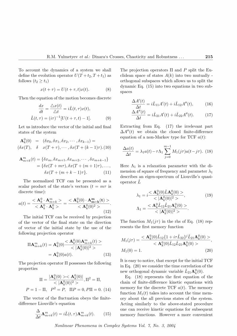
The time series of the orthogonal variables W0

(Fig. 2(a)), W1 (Fig. 2(b)), W2 (Fig. 2(c)), W3

(Fig. 2(d)) for chaotic dynamics of solar activityare submitted in Fig. 2. As the initial time se-

ries the variable W0 forms a dynamic noise. Theanalysis of the time series of a variable W0 shows,that the most appreciable fluctuations of this dy-namic variable relate on the maxima of solar ac-tivity. The bursts of solar activity are located onquasiequal intervals from each other. It testifiesabout the quasi-periodicity changes of Sun activ-ity during all research time interval. The timeseries of the first three variables W1, W2, W3 aresymmetric in regard to the axis of abscissa. Thefive dynamic peaks falls at five full cycles (for theperiod with 1940 on 2001). We can note the bifur-cation in the each dynamic peak and this indicateon the existence of two peaks during maximumof the solar activity in each cycle (Fig. 1(b)).The kind of each separate maximum resemblesoutwardly a sea wave. At first, the wave gathersforce, then reaches a point of the maximal height,weakens a little, then again gathers force and fallsdown finally.

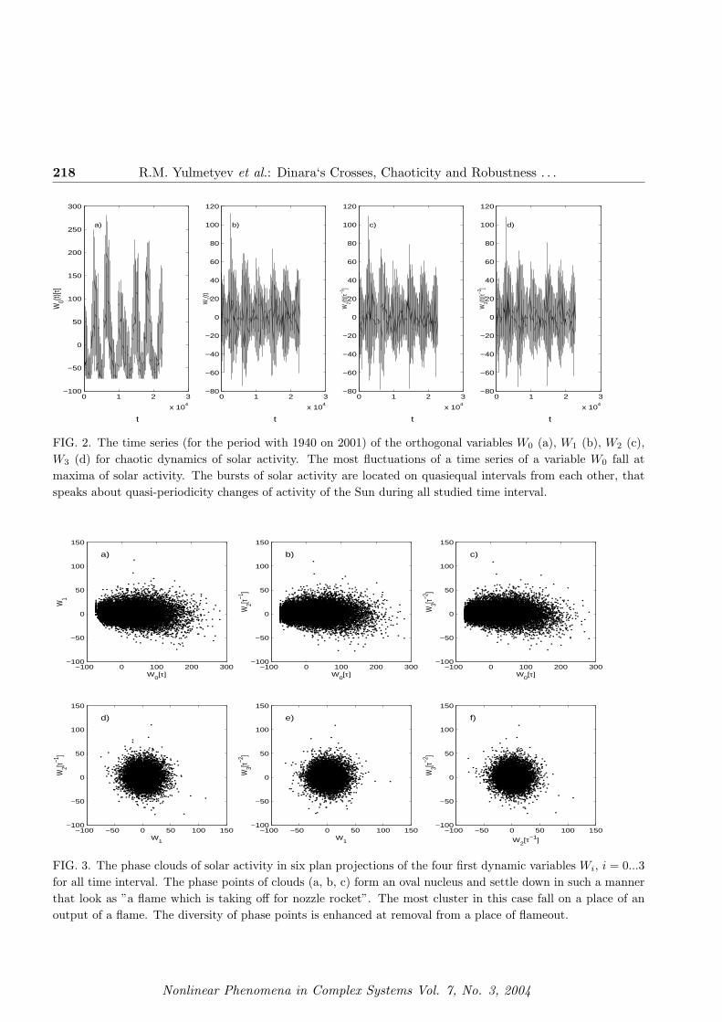
In Fig. 3 phase clouds in six plan projections ofthe four first dynamic variables Wi, i = 0, . . . , 3are submitted for cycles of solar activity. Theasymmetry of phase clouds concerning the centerof coordinates on the three first phase portraits isobserved. The phase points form an oval nucleusand settle down in such a manner that remind”a flame which is taking off for nozzle rocket”.The most cluster in this case fall on a place of anoutput of a flame. The diversity of phase pointsis enhanced at removal from a place of flameout.On the last three phase portraits are apprecia-ble central nucleuses which are symmetric aboutcenter of coordinates.

In Fig. 4 the power spectra of TCF µ0(ν)and the three junior functions memory µi(ν), i =1, 2, 3 for the chaotic dynamics of solar activityare submitted. The frequency spectra are givenin doubly logarithmic scale for a more detailedanalysis of the data. The power spectra of TCFµ0(ν) has fractal dependence on the middle andhigh frequencies. The small burst of power onfrequency ν = 4 ∗ 10−2f.u. (1f.u. = 1/τ) dividesarea of these frequencies where τ there is time ofdiscretization, τ = 1 day. A distinct peak withperiod 25-27 days (the frequency ν = 4∗10−2f.u.)



0 1 2 3

x 104

−100

−50

0

50

100

150

200

250

300

t

W0(t)

[τ]

a)

0 1 2 3

x 104

−80

−60

−40

−20

0

20

40

60

80

100

120

t

W1(t)

b)

0 1 2 3

x 104

−80

−60

−40

−20

0

20

40

60

80

100

120

t

W2(t)

[τ−1]

c)

0 1 2 3

x 104

−80

−60

−40

−20

0

20

40

60

80

100

120

t

W3(t)

[τ−2]

d)

FIG. 2. The time series (for the period with 1940 on 2001) of the orthogonal variables W0 (a), W1 (b), W2 (c),W3 (d) for chaotic dynamics of solar activity. The most fluctuations of a time series of a variable W0 fall atmaxima of solar activity. The bursts of solar activity are located on quasiequal intervals from each other, thatspeaks about quasi-periodicity changes of activity of the Sun during all studied time interval.

−100 0 100 200 300−100

−50

0

50

100

150

W0[τ]

W1

a)

−100 0 100 200 300−100

−50

0

50

100

150

W0[τ]

W2[τ−1

]

b)

−100 0 100 200 300−100

−50

0

50

100

150

W0[τ]

W3[τ−2

]

c)

−100 −50 0 50 100 150−100

−50

0

50

100

150

W1

W2[τ−1

]

d)

−100 −50 0 50 100 150−100

−50

0

50

100

150

W1

W3[τ−2

]

e)

−100 −50 0 50 100 150−100

−50

0

50

100

150

W2[τ−1]

W3[τ−2

]

f)

FIG. 3. The phase clouds of solar activity in six plan projections of the four first dynamic variables Wi, i = 0...3for all time interval. The phase points of clouds (a, b, c) form an oval nucleus and settle down in such a mannerthat look as ”a flame which is taking off for nozzle rocket”. The most cluster in this case fall on a place of anoutput of a flame. The diversity of phase points is enhanced at removal from a place of flameout.



represents the rotation of the Sun as viewed fromEarth [16]. In the field of low frequencies thesharp break which maximum falls to the fre-quency ν = 3 ∗ 10−4f.u. is observed. The largepeak at frequency 0.0003f.u. on the left in Fig.4 corresponds to the decadal solar activity cycle.Between these two peaks the spectrum displaysa power-law dependence on scale [16]. The fre-quency behavior of the three junior memory func-tions µi(ν), i = 1, 2, 3 has an identical structure.In the field of low frequencies the sharp breakwith a characteristic maximum is found. Theburst on the certain frequency ν = 4 ∗ 10−2f.u.divides the areas of middle and high frequencies.

10−4

10−3

10−2

10−1

10−2

100

102

104

106

108

ν [1/ τ]

µ 0 (

ν)[τ

2]

a)

10−4

10−3

10−2

10−1

10−4

10−2

100

102

104

ν [1/ τ]

µ 1 (

ν)[τ

2]

b)

10−4

10−3

10−2

10−1

10−2

10−1

100

101

102

103

104

ν [1/ τ]

µ 2 (

ν)[τ

2]

c)

10−4

10−3

10−2

10−1

10−2

10−1

100

101

102

103

104

ν [1/ τ]

µ 3 (

ν)[τ

2]

d)

FIG. 4. The power spectra of TCF µ0(ν) (a) andthe three junior memory functions µi(ν), i = 1, 2, 3for chaotic dynamics of solar activity. The frequencyspectra are given in doubly logarithmic scale for amore detailed analysis of the data. The areas of mid-dle and high frequencies are divided by small burst ofpower on frequency ν = 4 ∗ 10−2f.u. on the all dia-grams.

In Fig. 5 the spectra of the first three points ofstatistical non-Markovity parameter εi(ν), wherei = 1, 2, 3 are presented. The parameter ε1(ν) onthe frequency ν = 0 accept a value 95 that tes-tifies about strong markovization and amplifica-tion of chaoticity of the process. The Markovianbursts on the frequencies ν = 0, 0.04, 0.07f.u. areobserved and they reach the values 95, 23 and110. The second burst corresponds to a maxi-

mum (in point of peak on low frequencies) in thepower spectra of initial TCF (Fig. 4(a)). Thespectrum of non-Markovity parameter for the sec-ond point ε2(ν) is symmetric about the direct lineε2(ν) =1. In the frequency spectrum of the thirdpoint of the statistical non-Markovity parameterε3(ν) the characteristic minimum with peaks inthe beginning and the end of the frequency de-pendencies is appreciable. In the spectra ε2(ν),ε3(ν) at the frequency ν = 0.04, 0.07f.u. charac-teristic bursts are observed. The first peaks cor-respond to the maxima of low-frequency burstsin the power spectra µ1(ν), µ2(ν).

0 0.1 0.2 0.3 0.4 0.50

20

40

60

80

100

120

ν [1/ τ]

ε1 (

ν)

a)

0 0.1 0.2 0.3 0.4 0.50

0.2

0.4

0.6

0.8

1

1.2

1.4

1.6

ν [1/ τ]

ε2 (

ν)

b)

0 0.1 0.2 0.3 0.4 0.50.7

0.8

0.9

1

1.1

1.2

1.3

1.4

ν [1/ τ]

ε3 (

ν)

c)

FIG. 5. The spectra of first three points of the statis-tical non-Markovity parameter εi(ν), where i = 1, 2, 3.At the frequency ν = 0 the parameter ε1(ν) (a)achieves value 60 that speaks about strong markoviza-tion of studied process and transition in a mode ofMarkov chaoticity. The Markovian bursts on the fre-quencies ν = 0.04, 0.07f.u. are observed and theyreach values 23, 110. The first peaks correspond tomaximum of peak on low frequencies in the powerspectra of the initial TCF.

Recently the correlation analysis has experi-enced a marked lack of information concerningthe object under study. Procedure of local av-eraging of various parameters allows to examinethe separate hidden properties of objects studied.The characteristic feature of the usual correlationanalysis is the fact that the greatest possible setof signals is required for the qualitative analysisof the properties of the object of the research.At longer sample of such signals it is possible toreceive more exact information with the help of



the correlation analysis. Let us take a randomnon-Markov process as an example. This pro-cess consists of sequence of alternating randomstates. Thus, the problem of extraction of moreinformation not only about the common processbut about various single dynamic states of a sys-tem arises. In this case the use of the correlationanalysis for the whole time series will be ineffi-cient. The processing of the signals is necessaryfor separate local sites of the full time series. Itwill allow to consider the properties of separatedynamic states of the system.

Hereinafter a new method of data processingbased on the local averaging of kinetic and re-laxation parameters is offered. This method al-lows to consider the properties of separate non-stationary states of the systems. The idea of amethod is the following: there exists an initialdata set. Let’s take a sampling in length N ofsignals and to calculate its kinetic and relaxationparameters. Then the operation of ”step-by-stepshift to the right” for one time interval is carriedout. The kinetic and relaxation parameters arecalculated again. The ”step-by-step shift to theright” will continued to the end of time series.Such locally averaged parameters have high sen-sitivity to the effects of intermittency and non-stationarity. If the initial time series has someirregularity, it is instantly reflected in the behav-ior of the locally averaged parameters.

The use of this method requires the choice ofthe optimal length of a sampling which enablesto receive the most trustworthy information. Ifa sampling is too short, so noise effects does notallow to receive qualitative information. Besideswith a short length sampling we have significanterrors. On the other hand at great length of asampling locally averaged parameters lose ”sensi-tivity” necessary for the study. As a result of thestudy of different lengths of local sampling wehave received the optimal length compose 100-120 points. Further proofs of all aforesaid will begiven below.

In Fig. 6 the time dependence located kinetic(λ1, λ2, λ3) and relaxation (Λ1, Λ2) parameters issubmitted. Procedure of localization allows to re-

ceive more detailed representation about a phys-ical nature of researched object. The located pa-rameters have ”increase”of sensitivity to featuresof local states. The local parameters reflect sep-arate local changes which occur in investigatedobject. The detailed analysis of the time depen-dence of the local kinetic parameter λ1(t) allowsto show the six most significant changes. The be-havior of parameter changes sharply in the case ofoccurrence of minima of solar activity. Equidis-tance and periodicity of similar changes followsfrom here. The similar picture is observed and forother local parameters. The parameters λ1 andΛ1 have an maximal sensitivity among all localparameters. The parameters λ1, λ2, λ3 possessnegative values on all the time interval whereasΛ1, Λ2 have an both positive and negative numer-ical values.

4.2 The study of some features ofseparate solar cycles

The analysis of qualitative results of data pro-cessing for chaotic dynamics of separate cycles ofsolar activity (18) allows to reveal the followingregularity. In the most cases the maximum of so-lar activity has an complex structure on which isemerged no one, but two peaks. The first peakachieves the greatest amplitude in addition. Theamplitude of the first peak in a maximum of eachcycle is defined by special ”indicator” which is thefirst point of the non-Markovity parameter ε1(ν).This parameter constitute an informative mea-sure of chaoticity or regularity of the processes inreal object.

In Fig. 7 the power spectra of TCF µ0(ν)and the three junior memory functions µi(ν), i =1, 2, 3 for chaotic dynamics for one of cycles of so-lar activity are submitted. The frequency spectraof initial TCF µ0(ν) are submitted in doubly log-arithmic scale. Fractal dependence of the powerspectra has been collapsed by the small burst onthe frequency ν = 4 ∗ 10−2f.u. (the 25-27 dayperiod of the rotation of the Sun as viewed fromEarth). The power spectra of three junior mem-ory functions µi(ν), i = 1, 2, 3 are submitted in a



0 0.5 1 1.5 2 2.5

x 104

−0.4

−0.2

0

0.2

t

λ1(t)

a)

0 0.5 1 1.5 2 2.5

x 104

−1.5

−1

−0.5

0

t

λ2(t)

b)

0 0.5 1 1.5 2 2.5

x 104

−1.5

−1

−0.5

t

λ3(t)

c)

0 0.5 1 1.5 2 2.5

x 104

−0.4

−0.2

0

0.2

t

Λ1(t)

d)

0 0.5 1 1.5 2 2.5

x 104

−0.5

0

0.5

t

Λ2(t)

e)

1 2 3 4 5 6

1 2 3 4 5 6

FIG. 6. The time dependence of local kinetic (λ1, λ2,λ3) and relaxation (Λ1, Λ2) parameters. The anal-ysis of the time dependence of the located kineticparameter λ1(t) allows to show the six most signifi-cant changes. The behavior of the parameters sharplychanges in case of an ascertainment of minima of so-lar activity. Equidistance and periodicity of similarchanges follows from here. The behavior of other pa-rameters is similar.

usual frequency scale. In the field of low frequen-cies a few consistently going bursts are discov-ered, among which the greatest attention is nec-essary for giving of the first burst at frequency0.04f.u. The amplitude of the zero burst (at zerofrequency) displays amplitude of the first peak ofa maximum of solar activity.

The complex structure of power spectra ap-pears in frequency dependence of the first three

10−3

10−2

10−1

10−2

100

102

104

106

ν [1/ τ]

µ 0 (

ν)[τ

2]

a)

0 0.1 0.2 0.3 0.4 0.50

20

40

60

80

100

120

140

ν [1/ τ]

µ 1 (

ν)[τ

2]

b)

0 0.1 0.2 0.3 0.4 0.50

10

20

30

40

50

60

70

80

ν [1/ τ]

µ 2 (

ν)[τ

2]

c)

0 0.1 0.2 0.3 0.4 0.50

10

20

30

40

50

60

ν [1/ τ]

µ 3 (

ν)[τ

2]

d)

FIG. 7. The power spectra of the TCF µ0(ν) and thefirst three junior memory functions µi(ν), i = 1, 2, 3for chaotic dynamics for one of cycles of solar activ-ity - 18. The frequency spectra initial TCF µ0(ν) aregiven in doubly logarithmic scale. Fractal dependenceof the power spectra is broken small burst on the fre-quency ν = 4 ∗ 10−2f.u. In the field of high frequen-cies a condensation of spectral lines is appreciable.The power spectra of three junior memory functionsµi(ν), i = 1, 2, 3 are submitted in a usual frequencyscale. In the field of low frequencies a few consistentlygoing bursts are discovered (among which the great-est attention is necessary for first burst at frequency0.04f.u.). The amplitude of the zero burst (at zerofrequency) displays amplitude of the first peak of amaximum of solar activity.

points of the statistical spectrum non-Markovityparameter εi(ν), i = 1, 2, 3, see Fig. 8. Onthe zero frequency appreciable amplification ofMarkov effects is observed in non-Markovity pa-rameter ε1(ν). The amplitude of this burst de-fines the greatest amplitude of the first maximum.The greater is the amplitude of the first point, thegreat becomes amplitude of the first maximum ofsolar activity. At the greater value of amplitudeof the first point of non-Markovity parameter onzero frequency the amplitude of the first maxi-mum of solar activity also accept greater value.On the frequency ν = 0.04f.u. the small peakwhich reflects the appropriate low-frequency con-tribution to the power spectra of initial TCF ap-pears (the 25-27 day period). The structure of the



spectrum of non-Markovity parameter for the sec-ond point ε2(ν) reflects the structure of the powerspectrum of the first memory function µ1(ν). Inthe field of low frequencies there are peaks withmaxima which are coincided with the appropri-ate maxima of bursts in the power spectra of thememory function µ1(ν). In the frequency behav-ior of the third point of non-Markovity parameterε3(ν) one can discover the crest with amplitudecorresponding to the amplitude of burst in thepower spectrum of the second memory functionµ2(ν).

0 0.1 0.2 0.3 0.4 0.50

10

20

30

40

50

60

70

80

ν [1/ τ]

ε1 (

ν)

a)

0 0.1 0.2 0.3 0.4 0.50.7

0.8

0.9

1

1.1

1.2

1.3

1.4

ν [1/ τ]

ε2 (

ν)

b)

0 0.1 0.2 0.3 0.4 0.50.8

0.85

0.9

0.95

1

1.05

1.1

1.15

1.2

1.25

ν [1/ τ]

ε3 (

ν)

c)

FIG. 8. The spectra of the first three points of thenon-Markovity parameter εi(ν), i = 1, 2, 3 for chaoticdynamics of one of the cycles of solar activity. Fromthe dependence of the non-Markovity parameter ε1(ν)(a) near to zero frequency the appreciable amplifica-tion of Markov effects is observed. The amplitude ofthis burst defines the most significant amplitude of thefirst peak of a maximum of solar activity. The greateramplitude of the first point of non-Markovity param-eter on zero frequency corresponds to the greater am-plitude of the first peak of solar activity. The fre-quency behavior of the second and third points ofnon-Markovity parameter reflects frequency structureof power spectra of the first and second memory func-tions.

4.3 The definition of chaoticity andregularity of the processesproceeding on the Sun

Phase clouds in six plane projections of dynamicorthogonal variables for typical year of maximum(1947) (Figs. 9 (A-F)) and year of minimum

(1986) (Figs. 9 (a-f)) of solar activity are sub-mitted on Fig. 9. The represented diagrams arecharacteristic for all years with the maximal andminimal solar activity. Thus further analysis willbe is made only for these typical cases. The phasepoints in the case of a maximum forms a nucleusin the form of the oval curve(Fig. 9 (A)). In com-parison with other years of the cycle the intervalof scattering of the phase points along the hori-zontal axis is maximal and equal to 280 τ . Thephase points per year with a minimum of solar ac-tivity (Fig. 9 (a)) are dissipated from the center.On the left side of the phase cloud in a plane(W0,W1) the phase points are built along twolines which form the certain blunt angle. Theselines appear in the phase clouds two - three yearsprior to a minimum of solar activity. On the fol-lowing phase clouds of a point are built clearlyalong a direct line. The rest of phase points aredistributed in the right half-plane concerning thisdirect line. On the last three phase portraits thephase points form symbolic ”Dinara’s Crosses”with the center in the beginning of coordinates.These crosses, the distinctive for the one yearwith the minimal solar activity, has received thename ”Dinara’s Crosses”, in honor of the girl -student who was the first to discover this phe-nomena. We have revealed that the such kindof the phase clouds is characteristic for any yearwith the minimum of solar activity.

At observation of the phase clouds in the samescale the following picture appears. For any yearwith the greatest solar activity phase points arescattered on a phase plane as much as possible. Inthe following year the phase points gather closerto the center and occupies a more correct circu-lar area of a plane. The next year points aregrouped even more around the center. Per yearof the minimum of solar activity the phase pointscreate an almost ideal circle as much as possiblecompressed to the center.

In Fig. 10 the first three points of the non-Markovity parameter εi(ν), where i = 1, 2, 3 onthe zero frequency for all time interval is shown.Thus parameter ε1(0) gets special physical value.This point is the original ”indicator” of manifes-



−200 −100 0 100 200−100

0

100

200

W0[τ]

W1

A)

−200 −100 0 100 200−100

0

100

200

W0[τ]

W2[τ

−1]

B)

−200 −100 0 100 200−100

0

100

200

W0[τ]

W3[τ

−2]

C)

−100 −50 0 50 100 150−100

0

100

200

W1

W2[τ

−1]

D)

−100 −50 0 50 100 150−100

0

100

200

W1

W3[τ

−2]

E)

−100 −50 0 50 100 150−100

0

100

200

W2[τ−1]

W3[τ

−2]

F)

−20 0 20 40 60 80−50

0

50

W0[τ]

W1

a)

−20 0 20 40 60 80−20

0

20

40

W0[τ]

W2[τ

−1]

b)

−20 0 20 40 60 80−50

0

50

W0[τ]

W3[τ

−2]

c)

−40 −20 0 20 40−20

0

20

40

W1

W2[τ

−1]

d)

−40 −20 0 20 40−50

0

50

W1

W3[τ

−2]

e)

−20 −10 0 10 20 30−50

0

50

W2[τ−1]

W3[τ

−2]

f)

FIG. 9. The phase clouds in six plane projections of dynamic orthogonal variables for typical year with maximumof solar activity (1947) (A-F) and with minimum of solar activity (1986) (a-f). In the case of maximum the phasepoints are formed as a nucleus in the form of oval (A). The straggling of the phase points along abscissa axes ismaximal as compared with other years of the cycle. The phase points for one year with minimum of solar activity(a) are approached to the center. On the left side of the phase cloud in a plane (W0,W1) the phase points arebuilt along two lines which form the certain blunt angle. On the last three phase portraits the phase points formsymbolical ”Dinara’s Crosses” with the center in the beginning of coordinates.

tation of chaoticity or regularity. The values ofthis point are minimal within maxima and min-ima years of solar activity and may range from 4to 8. Per years appropriate growth phases and re-cession of solar activity, parameter ε1(0) achievesvalue 15-26. At the same time, this parameterdefines the quantitative measure of the chaoticityof the processes on the Sun. The greater numer-ical value is of this parameter, the greater is achaoticity. Thus, with removal from the mini-mum or the maximum of solar activity the ran-domness of the processes on the Sun amplifies.It is connected to the greater variability of set of

the various processes on the Sun. Specifically, thefollowing years: 1956 (ε1(0) =26.1), 1984 (26.3),1988 (24.3), 1992 (20.1), 1998 (19.6) differ by thegreatest chaoticity. These years correspond toyears of phases of growth or slump for solar activ-ity. It means, that most suggestive events duringsolar cycle occur in these phases. The greatestrobustness and appreciable non-Markovity effectsare characteristic for the next years: 1954 (4.78),1958 (3.7), 1964 (4.8), 1968 (3.98), 1980 (3.8). Ifto compare these dates with those in table of thesolar activity cycles (Ishkov, 2001) then one cannote, that minimum of 18 cycle was in 1954 year,



FIG. 10. The first three points of non-Markovity parameter εi(ν = 0) where i = 1, 2, 3, on zero frequencyare calculated for the one year sampling and in aggregate for all time interval are given. The first point ofnon-Markovity parameter is original ”indicator” of display of randomness or regularity. The values of this pointwithin maxima and minima of solar activity are minimal. Per years which are sandwiched between maxima andminima of the solar activity, numerical values of size ε1(0) are maximal. The greater is numerical value of thisparameter, the greater is a chaoticity. Thus, chaoticity of the processes on the Sun, with removal from minimumor maximum of solar activity intensifies.

20th maximum was in 1968 year etc. The com-plex frequency structure of the first point of non-Markovity parameter is reflected in frequency de-pendence ε2(0), ε3(0) also.

5 Conclusions

In this paper a method of the correlation analysisof dynamics of solar activity on the basis of thetheory discrete non-Markov processes is offered.The developed method allows for discreteness ofvarious processes on the Sun, effects of long-rangememory and aftereffect, and also effects of dy-namic alternation. It enables us to visualize andconsider a series of the regularities which ariseowing to periodicity and cyclicity of the solar ac-tivity. The regularities connected with cyclicityof solar activity, are reflected in the phase por-traits of the first four dynamic orthogonal vari-

ables. The characteristic compression and the ex-pansion of the phase clouds, recalling a pulsationof heart is observed at that. The phase clouds,the most dense in minimum, are increased on vol-ume in 3-4 times at a period of the maximum ofsolar activity.

The physical non-Markovity parameter εi(ν)where i = 1, 2, 3 represents the quantitative mea-sure of chaoticity and a regularity of the randomprocesses on the Sun. Per years between min-ima and maxima the chaoticity of the stochasticprocesses connected to solar activity, is maximal.It is connected with greater variability of vari-ous dynamic states of system. It corresponds toyears of reconstruction of dynamic state of theSun. The analysis of fluctuations in the spectra ofmemory functions and frequency dependencies ofthe first three points of statistical non-Markovityparameter testifies an opportunity of use of our



method for forecasting of solar activity. Points ofthe first phase portraits per years with the min-imal solar activity generate two lines forming ablunt angle. Distinctive Dinara’s Crosses whichcan be considered as a predictors of the appear-ance of minimum of solar activity appear in thephase clouds just at this period. The similar con-struction of the phase clouds emerges as two -three years prior to a minimum of solar activity.The dynamic peaks on the zero frequency at fre-quency spectrum of the time correlation functionµ0(ν) and frequency behavior of the first pointof the non-Markovity parameter ε1(ν), determinethe amplitude of the first dynamic peak per yearwith the maximal solar activity.

The locally averaged kinetic and relaxation pa-rameters of chaotic dynamics of solar activity al-low to study statistical features of the processesconnected to solar activity in more details. Thelocal time series reflect internal features of cyclic-ity of solar activity that helps to study the reg-ularity afforded by solar activity. The offeredmethod allow to find the features inherent in anycycle of solar activity at the big volume of experi-mental data. Physical feature of the local param-eters is that the any irregularity arising in theinitial time series, is instantly reflected in localtime behavior of studied parameters. Procedureof local averaging allows to find out properties ofsystem which are latent for the usual correlationanalysis. Because of use of the given procedurethe structure of any cycle of solar activity be-comes more obvious. It means an opportunityof the calculation of the detailed quantitative pa-rameters of various dynamic modes of solar activ-ity. We plan to use this technique for the studyingof other manifestations the solar activity on theEarth.

6 Acknowledgements

This work supported by the RHSF (Grant N 03-06-00218a), RFBR (Grant N 02-02-16146, 03-02-06084, 03-02-96250) and CCBR of Ministryof Education RF (Grant N E 02-3.1-538, A03-

2.9-804). The authors thanks Professor J. K.Lawrence for valuable comments and remarks andacknowledge Dr. L.O. Svirina for technical assis-tance.

References

[1] R. M. Yulmetyev, P. Hanggi, and F. M. Gafarov.Phys. Rev. E62, 6178 (2000).

[2] R. M. Yulmetyev, F. M. Gafarov, P. Hanggi, R.R. Nigmatullin, and Sh. Kayumov. Phys. Rev.E64, 066132 (2001).

[3] R. M. Yulmetyev, P. Hanggi, and F. G. Gafarov.Phys. Rev. E65, 046107 (2002).

[4] S. K. Solanki. A&ARev. 11, 153 (2003).[5] N. O. Weiss, and S. M. Tobias. Spase Sci. Rev.

94, 99 (2000).[6] N. Kleeorin, K. Kuzanyan, D. Moss, I. Ro-

gachevskii, D. Sokoloff, and H. Zhang. astro-ph/0304232 (2003).

[7] I. I. Salakhutdinova. Astronomy and Geodesy inNew Millenium, ed. N. A. Sakhibullin (Kazan:DAS), p. 291, (2001).

[8] S. Watari. Solar Phys. 168, 513 (1996).[9] U. M. Leiko. Selected Problems of the Astron-

omy, ed. S. A. Yazev (Irkutsk: Oblmashinform),p. 150 (2001)(in Russian).

[10] M. N. Khramova, E. V. Kononovich, and S.A. Krasotkin. Solar System Research. 36, 507(2002).

[11] M. G. Ogurtsov, Yu. A. Nagovitsyn, and G. E.Kocharov. Solar Phys. 211, 371 (2002).

[12] S. Watari. Solar Phys. 163, 259 (1996).[13] N. Jevtic, J. S. Schweitzer, and C. J. Cellucci.

Astron. Astrophys. 379, 611 (2001).[14] M. Carbonell, R. Oliver and J. L. Ballester As-

tron. Astrophys. 290, 983 (1994).[15] H. Isliker, L. Vlahos, A.O. Benz, and A. Raoult.

Astron. Astrophys. 336, 371 (1998).[16] J. K. Lawrence, A. C. Cadavid, and A. A. Ruz-

maikin. ApJ. 455, 366 (1995).[17] Q. Zhang. Solar Phys. 178, 423 (1998).[18] J. K. Lawrence, A. A. Ruzmaikin, and A. C.

Cadavid. Astrophys. J. 417, 805 (1993).[19] J. K. Lawrence, A. C. Cadavid, and A. A. Ruz-

maikin. Phys. Rev. E 51, 316 (1995).



[20] I. I. Salakhutdinova. Solar Phys. 181, 221(1998).

[21] I. I. Salakhutdinova. Solar Phys. 188, 377(1999).

[22] V. P. Mikhajlutsa. AZh. 70, 543 (1993).[23] K. J. Li, L. S. Zhan, J. X. Wang, X. H. Liu,

H. S. Yun, S. Y. Xiong, H. F. Liang, and H. Z.Zhao. Astron. Astrophys. 392, 301 (2002).

[24] M. Khramova, E. Kononovich, and S. Kra-sotkin. Solar variability: from core to outer fron-tiers, the 10th European Solar Physics Meeting,p. 145 (2002).

[25] V. I. Dmitrieva, K. M. Kuzanyan, and V. N.Obridko. Solar Phys. 195, 209 (2000).

[26] S. Sello. astro-ph/9906035 (1999).[27] S. Sello. astro-ph/0001042 (2000).[28] S. Sello. astro-ph/0010106 (2000).[29] S. Sello. Astron. Astrophys. 363, 311 (2000).

[30] R. Yulmetyev, N. Emelyanova, P. Hanggi, F.Gafarov, and A. Prokhorov. Physica. A 316,361 (2002).

[31] R. M. Yulmetyev, F. M. Gafarov, D. G. Yulme-tyeva, and N. A. Emelyanova. Physica. A 303,427 (2002).

[32] R. M. Yulmetyev, V. Yu. Shurygin, and T. R.Yulmetyev. Physica. A 242, 509 (1997).

[33] R. M. Yulmetyev, V. Yu. Shurygin, and N.R. Khusnutdinov. Acta Phys. Polon. B30, 881(1999).

[34] R. M. Yulmetyev, and N. R. Khusnutdinov. J.Phys. A27, 5363 (1994).

[35] R. M. Yulmetyev, R. I. Galeev, and V. Yu.Shurygin. Phys. Lett. A202, 258 (1995).

[36] V. N. Ishkov. Selected Problems of the Astron-omy. Ed. S.A. Yazev (Oblmashinform, Irkutsk,2001), p. 140 (in Russian).


Dinara‘s Crosses, Chaoticity and Robustness in … 2004 Nonlinear Phenomena in Complex Systems...

Documents

Transcript of Dinara‘s Crosses, Chaoticity and Robustness in … 2004 Nonlinear Phenomena in Complex Systems...