arX

iv:0

901.

2491

v2 [

hep-

th]

5 M

ar 2

009

DIAS–09–01HWM–09–01EMPG–09–01

Dimensional Reduction, Monopoles

and Dynamical Symmetry Breaking

Brian P. Dolan1,2 and Richard J. Szabo3

1School of Theoretical Physics, Dublin Institute of Advanced Studies10 Burlington Road, Dublin 4, Ireland

2Department of Mathematical Physics, National University of IrelandMaynooth, Co. Kildare, Ireland

3Department of Mathematics and Maxwell Institute for Mathematical SciencesHeriot-Watt University, Colin Maclaurin Building, Riccarton, Edinburgh EH14 4AS, U.K.

Email: bdolan@thphys.nuim.ie , R.J.Szabo@ma.hw.ac.uk

Abstract

We consider SU(2)-equivariant dimensional reduction of Yang-Mills-Dirac theory on manifoldsof the form M × CP 1, with emphasis on the effects of non-trivial magnetic flux on CP 1. Thereduction of Yang-Mills fields gives a chain of coupled Yang-Mills-Higgs systems on M with aHiggs potential leading to dynamical symmetry breaking, as a consequence of the monopolefields. The reduction of SU(2)-symmetric fermions gives massless Dirac fermions on M trans-forming under the low-energy gauge group with Yukawa couplings, again as a result of theinternal U(1) fluxes. The tower of massive fermionic Kaluza-Klein states also has Yukawa in-teractions and admits a natural SU(2)-equivariant truncation by replacing CP 1 with a fuzzysphere. In this approach it is possible to obtain exactly massless chiral fermions in the effectivefield theory with Yukawa interactions, without any further requirements. We work out the spon-taneous symmetry breaking patterns and determine the complete physical particle spectrum ina number of explicit examples.

1 Introduction

Various schemes have been used to suggest that the Higgs and Yukawa sectors of the standardmodel of particle physics may find their natural origin in a higher-dimensional gauge theory. Thenatural candidates for compact internal spaces in such Kaluza-Klein models are coset spaces G/H,as the action of the isometry group G can be elegantly compensated by gauge transformations insuch a way that the Lie derivative with respect to a Killing vector becomes a gauge generator.This provides a unification of the gauge and Higgs sectors in higher dimensions, while the cou-pling of fermions to the higher-dimensional gauge theory naturally induces Yukawa couplings afterdimensional reduction. The pioneering scheme realizing these constructions is called “coset spacedimensional reduction” [1, 2]. It has also been used more recently for the dimensional reductionof ten-dimensional supersymmetric gauge theories to four-dimensional field theories with softlybroken N = 1 supersymmetry [3], and for the reduction of superstring theories on nearly Kahlermanifolds [4]. On the other hand, a generic problem with Kaluza-Klein reductions has been thatthey are unable to generate chiral gauge theories, without some additional modifications [2, 5].

In coset space dimensional reduction, one imposes constraints on the higher-dimensional fieldswhich ensures that they are invariant under the G-action up to gauge transformations. Theyamount to studying embeddings of G or of its closed subgroup H in the gauge group of the higher-dimensional theory. The solutions of the constraints are then formally identified with the lowestmodes of the Kaluza-Klein towers of the fields, in a field expansion in harmonics on the compactcoset space G/H. However, this scheme does not seem to naturally allow for the incorporationof topologically non-trivial background fields on G/H which arise from gauging the holonomysubgroup H. It has been shown in [6] that, for certain coset spaces, the inclusion of non-trivialinternal fluxes can induce the chiral fermionic spectrum of quarks and leptons of the standardmodel.

In this paper we will study the dimensional reduction of gauge theories in a way which naturallyincorporates the topology of gauge fields on G/H. To distinguish our approach from the more stan-dard coset space techniques, we will refer to it as “equivariant dimensional reduction”. The generalformalism is developed in [7, 8] and has been used to describe vortices as generalized instantonsof higher-dimensional Yang-Mills theory [9]–[14], as well as to construct explicit SU(2)-equivariantmonopole and dyon solutions of pure Yang-Mills theory in four dimensions [15]. Although similarin spirit to the coset space dimensional reduction scheme, this approach systematically constructsthe unique field configurations on the higher-dimensional space which are equivariant with respectto the internal isometry group G and reduces Yang-Mills theory to a quiver gauge theory. Asin coset space dimensional reduction, there is a priori no relation between the gauge group G ofthe higher-dimensional field theory and the groups G or H, and the resulting gauge group of thedimensionally reduced field theory is a subgroup of G. This is in contrast to the usual Kaluza-Kleinreductions where the isometry group (or the holonomy group) is identified with the gauge group.

In the following we analyse in detail the simplest case where G = SU(2) and H = U(1), so thatthe internal space is the projective line CP 1. In this case the equivariant dimensional reduction ofgauge fields naturally comes with Dirac monopoles. We will emphasize the effects of the non-trivialmonopole background on the physical particle spectrum obtained from reduction of a Yang-Mills-Dirac theory. As usual, the mass scale of the dimensionally reduced field theory is set by the sizeof the internal space. We will obtain a Higgs sector of the lower-dimensional gauge theory with aHiggs potential that leads to dynamical symmetry breaking, as a direct consequence of the monopolecharges. We work out the complete physical particle content and masses for a variety of symmetryhierarchies, including one that entails the hierarchy SU(3) → SU(2) × U(1) → U(1) in which thesecond step is dynamical electroweak symmetry breaking. An induced Yukawa sector of the reducedfermionic field theory naturally emerges, again as a direct result of the internal fluxes. Starting

1

with massless fermions in higher dimensions, our dimensional reduction induces both massless andmassive fermions. In particular, it naturally allows for the reduction to massless chiral fermionswithout the imposition of any extra structure. In the case of higher spinor harmonic modes, whichgenerate massive fermions, we show that replacing the coset CP 1 with a fuzzy sphere gives a naturalSU(2)-equivariant truncation of the fermionic Kaluza-Klein tower while maintaining all quantitativefeatures of the continuous reduction, by using fuzzy spinor fields and a universal Dirac operator.Although the classes of models we present here are far from being phenomenologically viable ones,they provide a striking illustration of the utility of equivariant dimensional reduction and how thesystematic incorporation of topologically non-trivial gauge fields of the holonomy group can havedramatic implications on the physical particle spectrum of the reduced field theory, including anon-trivial vacuum selection mechanism.

The organisation of this paper is as follows. In §2 we describe some general aspects of theSU(2)-equivariant dimensional reduction of gauge and fermion fields over CP 1. In §3 we derivethe corresponding reduction of the pure massless Yang-Mills-Dirac action functional. In §4 and §5we work out large classes of dynamical symmetry breaking patterns, identifying the entire physicalparticle spectrum in each case. In §6 we summarize our findings, discuss some of the open problemsnot addressed in our analysis, and comment on the possibility of obtaining more physically realisticmodels using higher-dimensional homogeneous spaces G/H as the internal space.

2 Equivariant dimensional reduction over CP 1

In this section we will describe the dimensional reduction of gauge and fermion fields over theinternal coset space CP 1 ∼= SU(2)/U(1) which are invariant under the action of the SU(2) isometrygroup of CP 1. It is natural to allow for gauge transformations to accompany the spacetime SU(2)action [1, 2]. An elegant and systematic way to implement such a reduction is via a bundle theoreticapproach. For more details, see [8, 12].

2.1 SU(2)-equivariant bundles

By the inverse relations of induction and restriction [10], there is a one-to-one correspondencebetween SU(2)-equivariant complex vector bundles E → M := M × CP 1 and U(1)-equivariantcomplex vector bundles E → M , where SU(2) acts on the space M via the trivial action on themanifold M and by the standard (left) transitive action on the projective line CP 1 ∼= SU(2)/U(1).The U(1) subgroup of SU(2) also acts trivially on M . Assume that the structure group of theprincipal bundle associated to E is U(k). Imposing the condition of SU(2)-equivariance then meansthat we should look for representations of the isometry group SU(2) of CP 1 inside the U(k) structuregroup, i.e. for conjugacy classes of homomorphisms ρ : SU(2) → U(k). The dimensional reductionis thus given by k-dimensional unitary representations of SU(2). Up to isomorphism, for eachpositive integer r there is a unique irreducible SU(2)-module V r

∼= Cr of dimension r. Therefore,

for each positive integer m, the module

V =m⊕

i=0

V ki withm∑

i=0

ki = k (2.1)

gives a representation ρ of SU(2) inside U(k). The original generic U(k) gauge symmetry thenrestricts to the centralizer subgroup of the image ρ(SU(2)) in U(k),

U(k) −→m∏

i=0

U(ki) , (2.2)

2

which will be the low-energy gauge group of the dimensionally reduced field theory on M . Forstructure groups G other than U(k), the homomorphisms ρ : SU(2) → G, and hence the analogs ofthe restriction patterns (2.2), can be deduced from the Dynkin diagram of G.

The Lie algebra of SU(2) is generated by the three Pauli matrices

σ3 =

(1 00 −1

), σ+ =

(0 10 0

)and σ− =

(0 01 0

)(2.3)

with the commutation relations

[σ3 , σ±] = ± 2σ± and [σ+ , σ−] = σ3 . (2.4)

The Lie algebra of the U(1) subgroup of SU(2) is generated in this basis by σ3. For each p ∈ Z

there is a unique irreducible representation S p∼= C of U(1) given by ζ · v = ζp v for ζ ∈ S1 and

v ∈ S p. Since the manifold M carries the trivial action of the group U(1), any U(1)-equivariantbundle E → M admits a finite Whitney sum decomposition into isotopical components as [16]E =

⊕p E(p) ⊗ S p, where the sum runs over the set of eigenvalues for the U(1)-action on E and

E(p) →M are bundles with the trivial U(1)-action.

The corresponding SU(2)-equivariant bundle E →M × CP 1 is obtained by induction as

E = SU(2)×U(1) E , (2.5)

where the U(1)-action on SU(2)×E is given by h · (g, e) = (g h−1, h ·e) for h ∈ U(1), g ∈ SU(2) ande ∈ E. The σ3-action on E is described by the isotopical decomposition of E above. The rest of theSU(2) action, i.e. the actions of σ+ and σ− = σ+

†, follows from the commutation relations (2.4),which shows that the action of the generator σ+ on E(p) ⊗ S p corresponds to bundle morphismsE(p) → E(p+2), along with the trivial σ+-actions on the irreducible U(1)-modules S p. Introducethe standard Dirac p-monopole line bundle

Lp := SU(2)×U(1) S p (2.6)

over the homogeneous space CP 1, with Lp = L⊗p for p ≥ 0 and Lp = (L∨ )⊗(−p) for p < 0 whereL = L1. Then, for the induced complex vector bundle (2.5) over M ×CP 1 of rank k, the σ3-actionis given by the U(1)-equivariant decomposition

E =

m⊕

i=0

Ei with Ei = Ei ⊠ Lpi and pi = m− 2i , (2.7)

where Ei → M are complex vector bundles of rank ki with typical fibre the module V ki in (2.1),and Ei →M × CP 1 is the bundle with fibres

(Ei)(x,ξ)

=(Ei

)x⊗(Lpi)ξ

(2.8)

for x ∈M and ξ ∈ CP 1. On the other hand, the σ+-action is determined by a chain

0 −→ Em Φm−−→ Em−1Φm−1−−−−→ · · · Φ2−→ E1 Φ1−→ E0 −→ 0 (2.9)

of bundle morphisms between consecutive Ei’s. After fixing hermitean metrics on the complexvector bundles Ei → M, the σ−-action is described by reversing the arrows in (2.9) and using theadjoint bundle morphisms Φi

†.

3

This decomposition can be understood as follows. Given any finite-dimensional representationV of U(1), the corresponding induced, homogeneous hermitean vector bundle over the coset spaceCP 1 ∼= SU(2)/U(1) is given by the fibred product

V = SU(2)×U(1) V . (2.10)

Every SU(2)-equivariant bundle of finite rank over CP 1, with respect to the standard transitiveaction of SU(2) on the homogeneous space, is of the form (2.10). If V is irreducible, then U(1)is the structure group of the associated principal bundle. We consider those representations Vwhich descend from some irreducible representation of SU(2) by restriction to the U(1) subgroup.Then the bundle decomposition (2.7) is associated with the restriction of the irreducible SU(2)-representation of dimension r = m+ 1.

2.2 Invariant gauge fields

Let M be a manifold of real dimension d with local real coordinates x = (xµ) ∈ Rd, where the

indices µ, ν, . . . run through 1, . . . , d. The projective line CP 1 is a complex manifold with localcomplex coordinate y ∈ C and its conjugate y. The metric

ds2 = GAB dxA ⊗ dxB (2.11)

on M = M × CP 1 will be taken to be the direct product of a chosen riemannian metric on Mand the standard SO(3)-symmetric metric on CP 1 ∼= S2, where the indices A,B, . . . run over1, . . . , d+ 2. In the coordinates above it takes the form

ds2 = Gµν dxµ ⊗ dxν +4R2

(1 + y y)2dy ⊗ dy , (2.12)

where R is the radius of the sphere S2. We use conventions in which the coordinates x and yare dimensionless, while the line element (2.12) has mass dimension −2. More generally, one mayconsider warped compactifications of M with the same topology, but this doesn’t seem to add anynew qualitative features to our ensuing results.

Let A be a connection on the hermitean vector bundle E → M × CP 1 having the form givenby A = AA dxA in local coordinates (xA) and taking values in the Lie algebra u(k). We willnow describe the SU(2)-equivariant reduction of A on M × CP 1. The spherical dependences arein this case completely determined by the rank k of the bundle E and the unique (up to gaugetransformations) SU(2)-invariant connections ap on the monopole line bundles (2.6) having, inlocal complex coordinates on CP 1, the forms

ap =p

2 (1 + y y)(y dy − y dy) . (2.13)

The curvatures of these connections are

fp = dap = − p

(1 + y y)2dy ∧ dy , (2.14)

and their topological charges are given by the degrees of the complex line bundles Lp → CP 1 as

deg Lp =i

2π

∫

CP 1

fp = p . (2.15)

4

Related to the monopole fields are the unique, covariantly constant SU(2)-invariant forms of types(1, 0) and (0, 1) on CP 1 given respectively by

β =2 dy

1 + y yand β =

2 dy

1 + y y. (2.16)

They respectively form a basis of sections of the canonical line bundles K = L2 and K−1 = L−2,which are the summands of the complexified cotangent bundle T ∗

CP 1 ⊗ C = K ⊕K−1 over CP 1.The SU(2)-invariant Kahler (1, 1)-form on CP 1 is i

2 R2 β ∧ β.

With respect to the isotopical decomposition (2.7), the twisted u(k)-valued gauge potential Asplits into ki × kj blocks A =

(Aij)with Aij ∈ Hom

(V kj

, V ki

), which we write as

A = A(m)(x)⊗ 1 + 1k ⊗ a(m)(y) + φ(m)(x)⊗ β(y)−(φ(m)(x)

)† ⊗ β(y) (2.17)

where

φ(m) :=

0 φ1 0 . . . 00 0 φ2 . . . 0...

.... . .

. . ....

0 0 0 . . . φm0 0 0 . . . 0

(2.18)

while

A(m) :=m∑

i=0

Ai ⊗Πi and a(m) :=m∑

i=0

api ⊗Πi (2.19)

with Πi : E → Ei the canonical orthogonal projections of rank one onto the sub-bundles Ei, obeyingΠi Πj = δij Πi. The bundle morphisms Φi+1 := Ai i+1 = φi+1(x) ⊗ β(y) ∈ Hom(Ei+1, Ei) obeyΦm+1 = 0 = Φ0. The gauge potentials Ai ∈ u(ki) are connections on the hermitean vector bundlesEi → M . The bifundamental scalar fields φi+1 ∈ Hom(Ei+1, Ei) can be identified with sectionsof the bundles Ei ⊗ E∨

i+1 and transform in the representations V ki ⊗ V ∨ki+1

of the subgroupsU(ki) × U(ki+1) of the original U(k) gauge group. The gauge potential A given by (2.17) is anti-hermitean and SO(3)-invariant. All fields (Ai, φi+1) are dimensionless and depend only on thecoordinates x ∈M . Every SU(2)-invariant unitary connection A on M ×CP 1 is of the form givenin (2.17) (up to gauge transformations) [12, 10].

The curvature two-form F = dA+A∧A of the connection A has components which are givenby FAB = ∂AAB − ∂BAA + [AA,AB] in local coordinates (xA), where ∂A := ∂/∂xA. It also takesvalues in the Lie algebra u(k), and in local coordinates on M × CP 1 it can be written as

F = 12 Fµν dxµ ∧ dxν + Fµy dxµ ∧ dy +Fµy dxµ ∧ dy +Fyy dy ∧ dy . (2.20)

The calculation of the curvature (2.20) for A of the form (2.17) yields

F =(F ij)

with F ij = dAij +

m∑

l=0

Ail ∧ Alj , (2.21)

giving

F = F (m) + f (m) +[φ(m) , φ(m)

† ] β ∧ β +Dφ(m) ∧ β −(Dφ(m)

)† ∧ β (2.22)

where

F (m) := dA(m) +A(m) ∧A(m) and Dφ(m) := dφ(m) +[A(m) , φ(m)

], (2.23)

5

while f (m) = da(m) =∑

i fpi ⊗ Πi are the contributions from the monopole fields. We havesuppressed the tensor product structure pertaining to M × CP 1. From (2.22) we find the non-vanishing field strength components

F iiµν = F i

µν , (2.24)

F i i+1µy =

2

1 + y yDµφi+1 = −

(F i+1 iµy

)†, (2.25)

F iiyy = − 1

(1 + y y)2

(pi + 4φ†i φi − 4φi+1 φ

†i+1

), (2.26)

where F i = dAi +Ai ∧Ai = 12 F

iµν dxµ ∧ dxν are the curvatures of the bundles Ei →M , and

Dφi+1 = dφi+1 +Ai φi+1 − φi+1Ai+1 (2.27)

are bifundamental covariant derivatives.

The gauge field (2.22) can be formally identified with the lowest SU(2)-singlet mode in a har-monic expansion of forms on the internal space CP 1. Since the monopole fields are given byfpi = −pi

4 β ∧ β, it can be uniquely characterized by the requirement that it lives in the kernel ofthe covariant derivative operator on CP 1 in the monopole background, owing to the relations

dβ − a−2 ∧ β = 0 = dβ − a2 ∧ β . (2.28)

Equivalently, it is a zero mode of the covariant Laplace operator acting on forms on CP 1. As usualin Kaluza-Klein reductions, there is an infinite tower of massive harmonic modes on M which canalso be considered. Their contributions will not be analysed in this paper.

2.3 Symmetric spinor fields

Let M be a spin manifold. When d = dimR(M) is even, the generators of the Clifford algebraCℓ(M ×CP 1) obey

ΓA ΓB + ΓB ΓA = −2GAB12d/2+1 with A,B = 1, . . . , d+ 2 . (2.29)

The gamma-matrices in (2.29) may be decomposed as

{ΓA}

={Γµ,Γy,Γy

}with Γµ = γµ ⊗ 12 , Γy = γ ⊗ γy and Γy = γ ⊗ γy , (2.30)

where the 2d/2×2d/2 matrices γµ = −(γµ)† act locally on the spinor module ∆ (M) over the Cliffordalgebra bundle Cℓ(M) →M ,

γµ γν + γν γµ = −2Gµν12d/2 with µ, ν = 1, . . . , d , (2.31)

while

γ =i d/2

√G

d!ǫµ1···µd

γµ1 · · · γµd with (γ)2 = 12d/2 and γ γµ = −γµ γ (2.32)

is the corresponding chirality operator. Here ǫµ1...µdis the Levi-Civita symbol with ǫ12···d = +1.

The action of the Clifford algebra Cℓ(CP 1) on the spinor module ∆ (CP 1) is generated by

γy = − 1

2R(1 + y y) σ+ and γy =

1

2R(1 + y y) σ− . (2.33)

6

The treatment for d odd is similar.

The E-twisted Dirac operator on M = M × CP 1 corresponding to the equivariant gauge po-tential A in (2.17) is given by

D/ := ΓADA = γµDµ ⊗ 12 +(φ(m)

)γ ⊗ γy βy −

(φ(m)

)†γ ⊗ γy βy + γ ⊗D/

CP 1 , (2.34)

where

D/CP 1 := γyDy + γyDy = γy

(∂y + ωy +

(a(m)

)y

)+ γy

(∂y + ωy +

(a(m)

)y

)(2.35)

and ωy, ωy are the components of the Levi-Civita spin connection on the tangent bundle of CP 1.The E-twisted Dirac operator D/ := γµDµ on M is defined as

D/ = γµ(∂µ + θµ +

(A(m)

)µ

)with θµ = 1

2 θµνλ Σνλ , (2.36)

where θ = θµ dxµ is the spin connection on the tangent bundle of the manifold M and Σνλ are thegenerators of Spin(d). The operator (2.34) acts on spinors Ψ which are L2-sections of the bundle

Ψ =

(Ψ+

Ψ−

)∈

m⊕

i=0

(Ei ⊗∆(M)

)⊗(Lpi+1

Lpi−1

)(2.37)

over M×CP 1, where Lpi+1⊕Lpi−1 are the twisted spinor bundles of rank two over the sphere CP 1

and Ψ± are 2d/2+1 component spinors satisfying (12d/2 ⊗ σ3)Ψ± = ±Ψ±.

The equivariant dimensional reduction of massless Dirac spinors on M × CP 1 is defined withrespect to symmetric fermions on M . Similarly to the scalar fields φi+1(x) in (2.17), they act asintertwining operators connecting induced representations of U(1) in the U(k) gauge group, andalso in the spinor module ∆ (M) which admits the isotopical decomposition

∆ (M) =

m⊕

i=0

∆i ⊗ S pi with ∆i = HomU(1)

(S pi , ∆(M)

)(2.38)

obtained by restricting ∆ (M) to representations of U(1) ⊂ Spin(d) ⊂ Cℓ(M). The ∆i’s in (2.38)are the corresponding multiplicity spaces, and using Frobenius reciprocity they may be identifiedas

∆i = HomSU(2)

(∆(M) , L2

(CP 1,Lpi

)). (2.39)

The isotopical decomposition (2.38) is now realized explicitly by using (2.39) to construct sym-metric fermions on M as SU(2)-invariant spinors on M × CP 1. Analogously to the invariantgauge fields, they belong to the kernel of the Dirac operator (2.35) on CP 1, and after dimensionalreduction will be massless on M . One can write

D/CP 1 =

m⊕

i=0

D/ pi=

m⊕

i=0

(0 D/−

pi

D/+pi

0

), (2.40)

where

D/+pi

=1

2R

[(1 + y y) ∂y − 1

2 (pi + 1) y], (2.41)

D/−pi

= − 1

2R

[(1 + y y) ∂y +

12 (pi − 1) y

]. (2.42)

7

The operator (2.40) acts on sections of the bundle (2.37) which we write with respect to thisdecomposition as

Ψ =m⊕

i=0

(Ψ+

(pi)

Ψ−(pi)

), (2.43)

where Ψ±(pi)

are L2-sections of Lpi±1 taking values in ∆ (M) ⊗ V ki with coefficients dependingon x ∈M .

We need to solve the differential equations

D/+piΨ+

(pi)= 0 and D/−

piΨ−

(pi)= 0 (2.44)

for the spinors Ψ+(pi)

and Ψ−(pi)

in kerD/+pi

and kerD/−pi. By using the forms of the transition functions

for the monopole bundles, one easily sees that the only solutions of these equations which are regularon both the northern and southern hemispheres of S2 are of the form

Ψ+(pi)

=

−pi−1∑

ℓ=0

ψ(pi) ℓ(x)⊗ χ+(pi) ℓ

(y, y ) and Ψ−(pi)

= 0 for pi < 0 , (2.45)

Ψ−(pi)

=

pi−1∑

ℓ=0

ψ(pi) ℓ(x)⊗ χ−(pi) ℓ

(y, y ) and Ψ+(pi)

= 0 for pi > 0 , (2.46)

with

χ+(pi) ℓ

(y, y ) =yℓ

(1 + y y)−(pi+1)/2and χ−

(pi) ℓ(y, y ) =

y ℓ

(1 + y y)(pi−1)/2. (2.47)

The components, ψ(pi) ℓ(x) and ψ(pi) ℓ(x) with ℓ = 0, 1, . . . , |pi| − 1, are Dirac spinors on M which

form the irreducible representation V |pi|∼= C

|pi| of the group SU(2). This is of course consistentwith the fact that the index of the Dirac operator D/ p is equal to −p.

2.4 Harmonic spinor fields

In contrast to the bosonic sector, in the following we will find some noteworthy features of higherKaluza-Klein modes in the fermionic sector, so we shall describe them as well for completeness.They correspond to eigenspinors with non-zero eigenvalues in the spectrum of the Dirac operator(2.40) on CP 1, and are the only surviving fermions in the absence of the monopole background.The twisted spinor bundle given by Lpi+1 ⊕ Lpi−1 admits an infinite-dimensional vector space ofsymmetric L2-sections comprised of spinor harmonics Ψj,pi ∈ C

2, with pi = m− 2i [17]. They areeigenspinors of the Dirac operator D/ pi

, D/ piΨj,pi = ± 1

R λj,pi Ψj,pi, with eigenvalues

λj,pi =

√(j +

1− pi2

) (j +

1 + pi2

)(2.48)

each of multiplicitydj = 2j + 1 , (2.49)

where j is integral for odd pi and half-integral for even pi with j ≥ |pi|+12 . After dimensional reduc-

tion, this produces an infinite Kaluza-Klein tower of massive Dirac spinors on M . We decompose

8

the spinors (2.43) in this case as

Ψ+(pi)

=

∞∑

j=|pi|+1

2

2j∑

ℓ=0

ψ(j,pi) ℓ(x)⊗ χ+(j,pi) ℓ

(y, y ) ,

Ψ−(pi)

=∞∑

j=|pi|+1

2

2j∑

ℓ=0

ψ(j,pi) ℓ(x)⊗ χ−(j,pi) ℓ

(y, y ) , (2.50)

where χ±(j,pi) ℓ

are the chiral and antichiral spinors which are sections of Lpi±1, and form an L2-

orthogonal system on CP 1 normalized as∥∥χ±

(j,pi) ℓ

∥∥L2 = 4π R2 with

D/±piχ±(j,pi) ℓ

=1

Rλj,pi χ

∓(j,pi) ℓ

(2.51)

for each ℓ = 0, 1, . . . , 2j. The |pi| zero modes when |pi| ≥ 1 are recovered for j = 12 (|pi| − 1).

In contrast to the zero mode sector, this sector of the dimensionally reduced field theory containsan infinite number of modes on M , indicated by the infinite range of the angular momenta j. Inthis case a natural SU(2)-invariant way of reducing to a finite number of fermionic field degrees offreedom is to use a fuzzy sphere CP 1

F [18], truncated at some finite level j = jmax, as the internalspace. Dimensional reduction on the fuzzy sphere was considered in [19], although only for thecase m = 0 with no background monopole fields. Kaluza-Klein compactifications on CP 1

F includingnon-trivial internal magnetic flux are studied in [20], although in a different context than ours andin somewhat less generality.

The Dirac equation on the fuzzy sphere, and more generally on fuzzy CPN , has been anal-ysed in [21] and [22] respectively. The spectrum of the (universal) fuzzy Dirac operator includingmonopole backgrounds for a given maximal angular momentum jmax consists again of the eigen-values (2.48) as in the continuous case, except that now j ≤ jmax. The corresponding eigenspinorscan be constructed as finite-dimensional matrices. With L = jmax +

12 , positive chirality spinors

χ+(j,p) ℓ are complex matrices of dimension given by

(L− p

2

)×(L+ 1+ p

2

), while negative chirality

spinors χ−(j,p′ ) ℓ are matrices of dimension

(L+ 1− p′

2

)×(L+ p′

2

). By truncating at jmax = |pi|−1

2 ,

all spinor fields ψ(j,pi) ℓ and ψ(j,pi) ℓ vanish identically, and only the finitely many flavours of the

zero-mode symmetric spinors ψ(pi) ℓ and ψ(pi) ℓ of §2.3 survive the dimensional reduction.

3 Equivariant gauge theory of Kaluza-Klein modes

In this section we will work out the equivariant dimensional reduction of the pure massless Yang-Mills-Dirac action on M × CP 1. We will find that the role of the monopole fields on CP 1 isto induce a Higgs potential with dynamical symmetry breaking, as well as couplings to masslessspinors with Yukawa interactions from the zero modes of the Dirac operator D/

CP 1 . The mass scaleof the broken symmetry phase on M is determined by the size R of the internal coset space. Aninduced Yukawa sector of the low-energy effective field theory then emerges with the standard formof spontaneous symmetry breaking, containing both massless and massive fermions together withYukawa interactions with the physical Higgs fields. In particular, we will unveil the possibility ofobtaining exactly massless chiral fermions onM with Yukawa interactions, which can be interpretedas multiplets of left-handed quarks. Our approach thus avoids the extra requirements necessary forobtaining chiral fermions in the more conventional coset space dimensional reduction schemes [2].

9

3.1 Dimensional reduction of the Yang-Mills action

For the usual Yang-Mills lagrangian

LYM = − 1

4g2

√|G| trk×k FAB FAB (3.1)

on M =M × CP 1, one has

LYM = − 1

4g2

√|G| trk×k

[Fµν Fµν +

(1 + y y)2

2R2Gµν (Fµy Fνy + Fµy Fνy)

+1

8

((1 + y y)2

R2Fyy

)2 ]. (3.2)

The (d+2)-dimensional U(k) Yang-Mills coupling constant g has the standard mass dimension 1− d2

in order to make (3.2) dimensionless. The dimensional reduction of the corresponding Yang-Millsaction can be obtained by substituting (2.24)–(2.26) into (3.2) and performing the integral overCP 1 to arrive at the action

SYM :=

∫

M×CP 1

dd+2x LYM

=π R2

g2

∫

Mddx

√|G|

m∑

i=0

trki×ki

[(F iµν

)† (F i µν

)+

2

R2

(Dµφi+1

) (Dµφi+1

)†

+2

R2

(Dµφi

)† (Dµφi

)+

1

8R4

(pi + 4φ†i φi − 4φi+1 φ

†i+1

)2 ]. (3.3)

This result holds irrespectively of the signature of the chosen metric on the manifold M .

The action (3.3) defines a non-abelian Higgs model describing m interacting complex “rect-angular” scalar fields coupled to m + 1 non-abelian gauge fields. From (2.27) it follows that theU(1) factor in U(k) ≈ SU(k) × U(1) does not enter the bicovariant derivatives of φi+1, since anoverall U(1) factor cancels between the Ai and the Ai+1 terms. For the purposes of the ensuinganalysis in this subsection we can therefore focus on gauge group SU(k), though the overall U(1)subgroup would in general couple to fermions, in the fundamental representation of SU(k) for ex-ample. The decomposition (2.2) of the gauge group arising from the regular embedding of SU(2)is then modified to

SU(k) −→ U(1)m ×m∏

i=0

SU(ki) with

m∑

i=0

ki = k . (3.4)

The gauge coupling in d dimensions should have mass dimension 2− d2 , so we define g2 = g2/4π R2

as the d-dimensional gauge coupling constant. We then rescale φi → g Rφi and Ai → g Ai so that

the scalar fields and the gauge fields have the correct canonical dimensions for a d-dimensional fieldtheory (with dimensionless coordinates).

The action (3.3) can be succinctly rewritten as a matrix model by using the operators (2.18),(2.19) and (2.23) (with the rescalings φ(m) → g Rφ(m) and A(m) → gA(m)), together with

Σ(m) :=

m∑

i=0

pi Πi (3.5)

with respect to the decomposition (2.7). One then has

SYM =

∫

Mddx

√|G|

[trk×k

(14

(F (m)

)†µν

(F (m)

)µν+(Dµφ(m)

)† (Dµφ(m)

))+ V

(φ(m)

)], (3.6)

10

where the Higgs potential is given by

V(φ(m)

)=g2

2trk×k

(1

4g2 R2Σ(m) −

[φ(m) , φ(m)

†])2

. (3.7)

The Higgs potential (3.7) generically leads to dynamical symmetry breaking, as a direct consequenceof the non-trivial monopole background on CP 1. Its critical points are described by the matrixequations

φ(m) − 2g2R2[[φ(m),φ(m)

† ] , φ(m)

]= 0 , (3.8)

where we have used[Σ(m) , φ(m)

]= 2φ(m). When they exist, solutions of the equation

[φ(m) , φ(m)

†]=

1

4g2R2Σ(m) (3.9)

give the vacua of the Higgs sector of the field theory.

When k0 = k1 = · · · = km = n, so that the gauge symmetry restriction is given by

SU(k) −→ U(1)m × SU(n)m+1 with k = n (m+ 1) , (3.10)

an explicit solution of (3.9) is given by φ(m) = φ(m)0, where

φ0i =ζi

2g R

√i (m− i+ 1) 1n (3.11)

for i = 1, . . . ,m with ζi ∈ S1 independent phase factors. The phases ζi can be removed by aU(1)m gauge transformation in the unbroken symmetry phase. This solution breaks the gaugesymmetry of the d-dimensional field theory on M to SU(n). In the broken symmetry phase thereare mn2 massive gauge bosons, and mn2 physical Higgs fields which can be represented in termsof n × n hermitean matrices hi, i = 1, . . . ,m with φi = φ0i + hi. The corresponding Higgs masses,proportional to 1

R , can then be worked out by substitution into the Higgs potential (3.7), while thevector boson masses, also proportional to 1

R , can be worked out by substitution into the covariantderivative terms of the action (3.6). Note that for n = 1, the gauge symmetry reduction (3.10) isto the maximal torus of SU(m+ 1), and all gauge bosons become massive with no residual gaugesymmetry remaining. In the subsequent sections we will look at some explicit examples of suchmass generation in the field theory defined by (3.6).

3.2 Fermionic action for symmetric spinors

Using the gauged Dirac operator (2.34), we may define a euclidean fermionic action functional onthe space of L2-sections of the bundle (2.37) by

SD :=

∫

M×CP 1

dd+2x√

|G| Ψ†D/Ψ , (3.12)

where Ψ has canonical mass dimension 12 (d + 1). In lorentzian signature the adjoint spinor Ψ†

should be replaced by Ψ := 1√−G00

Ψ†Γ0. For definiteness, we shall only consider the case where the

spinor field Ψ transforms under the fundamental representation of the initial gauge group SU(k).Other fermion representations of SU(k) can be treated similarly.

One has

Ψ†(γ(φ(m)

)⊗ σ− + γ

(φ(m)

)† ⊗ σ+

)Ψ =

((Ψ+)

†(Ψ−)†

) (γ(φ(m)

)† (Ψ−)

γ(φ(m)

) (Ψ+)). (3.13)

11

Substituting (2.40)–(2.46), we see that (3.13) vanishes on symmetric spinors if m is even. On theother hand, if m is odd there is a surviving contribution from (2.45) and (2.46) when pi = ± 1. Forpi = −1 the single positive chirality zero mode is a section of the trivial line bundle L0 over CP 1,as is the single negative chirality zero mode for pi = +1. They are thus globally defined functionson CP 1, and hence are simply constants in (2.45) and (2.46) corresponding to SU(2)-singlets in thetrivial representation V 1. For these special cases the expression (3.13) produces Yukawa couplingsto the fields Ψ±

(∓ 1) on M .

After integration over CP 1, and the rescalings φi → g Rφi, ψ(pi) ℓ → (4π R2)−1/2 ψ(pi) ℓ, and

ψ(pi) ℓ → (4π R2)−1/2 ψ(pi) ℓ to give the scalar and fermion fields the correct canonical dimensionson M , the contribution from fermion zero modes on CP 1 to the action functional (3.12) is given by

S0D =

∫

Mddx

√|G|

[m∑

i=m+

|pi|−1∑

ℓ=0

(ψ(pi) ℓ

)†D/(ψ(pi) ℓ

)+

m−∑

i=0

|pi|−1∑

ℓ=0

(ψ(pi) ℓ

)†D/(ψ(pi) ℓ

)]

+g

2

∫

Mddx

√|G|

[(ψ(−1)

)†φ†m+

γ ψ(1) +(ψ(1)

)†φm+

γ ψ(−1)

], (3.14)

where m− =⌊m−12

⌋and m+ =

⌈m+12

⌉. The second term in (3.14) is present only when m is odd,

in which case m+ = m+12 . The fermion fields ψ(pi) ℓ and ψ(pi) ℓ for each ℓ = 0, 1, . . . , |pi| − 1, with

ψ(−1) := ψ(−1) 0 and ψ(1) := ψ(1) 0, transform in the fundamental representation of SU(ki). Recallthat this sector of the field theory onM is induced entirely by the non-trivial monopole backgroundon CP 1.

3.3 Fermionic action for spinor harmonic modes

For eigenspinors on CP 1 with non-zero eigenvalues, the term (3.13) produces an infinite chain ofYukawa couplings to the Higgs fields φi. After integration over CP 1, and again rescaling

φi → g Rφi , ψ(j,pi) ℓ →(4π R2

)−1/2ψ(j,pi) ℓ and ψ(j,pi) ℓ →

(4π R2

)−1/2ψ(j,pi) ℓ , (3.15)

the contributions from non-zero fermion modes on CP 1 with positive eigenvalues are given by∑mi=0 S

(pi)D with

S(pi)D =

∫

Mddx

√|G|

∞∑

j=jmin

2j∑

ℓ=0

[ (ψ(j,pi) ℓ

)† (D/ +

1

Rλj,pi γ

)ψ(j,pi) ℓ

+(ψ(j,pi) ℓ

)† (D/ +

1

Rλj,pi γ

)ψ(j,pi) ℓ

+g

2

(ψ(j,pi) ℓ

)†φ†i γ ψ(j,pi+2) ℓ +

g

2

(ψ(j,pi+2) ℓ

)†φi γ ψ(j,pi) ℓ

], (3.16)

where jmin = max( |pi|+1

2 , |pi+2|+12

). Again the fermion fields ψ(j,pi) ℓ and ψ(j,pi) ℓ, for each j ≥ jmin

and ℓ = 0, 1, . . . , 2j, transform in the fundamental representation of SU(ki).

Consider the truncation of the infinite tower of massive Dirac spinors on the fuzzy sphere CP 1F

at j = jmax as described in §2.4. The fuzzy analogue of the L2-norm∥∥χ±

(j,p) ℓ

∥∥L2 on CP 1 is the

matrix trace Tr[(χ±(j,p) ℓ

)†χ±(j,p) ℓ

], but observe that Tr

[(χ+(j,p) ℓ

)†χ−(j,p′ ) ℓ

]is also well-defined if and

only if p′ = p + 2 and this is exactly what is needed for the Yukawa couplings in (3.16). Notethat when i = 0, the Yukawa terms in (3.16) vanish because there is no fermion field ψ(j,m+2) ℓ.Similarly, the minimum value of the monopole charge pi in any spinor ψ(j,pi) ℓ is −m, when i = m, so

12

the fermion fields ψ(j,−m−2) ℓ are never present either. Hence ψ(j,m) ℓ and ψ(j,−m) ℓ have no Yukawacouplings, because they have no partners to which they can couple.

If the Higgs field φi acquires a non-zero vacuum expectation value φ0i by dynamical symmetry

breaking, then the fermion fields ψ(j,pi) ℓ and ψ(j,pi+2) ℓ acquire a mass matrix. For example, if one

takes k0 = k1 = · · · = km = n and φ0i = 1g R vi 1n as in (3.11), then the mass matrix for each

ℓ = 0, 1, . . . , 2j is

M f =1

R

(λj,pi

12 vi

12 vi λj,pi+2

), (3.17)

with eigenvalues

µ± =1

2R

(λj,pi + λj,pi+2 ±

√(λj,pi − λj,pi+2

)2+ |vi|2

). (3.18)

These masses are proportional to 1R . In general, it seems plausible that µ− could be very small,

or even zero, for specific symmetry breaking patterns, but we have not found an example wherethis happens. In this example all fermion fields transform in the fundamental representation of theunbroken gauge group SU(n) after spontaneous symmetry breaking.

Another interesting possibility arises when the metric on M is of lorentzian signature. Thenall adjoint spinors ψ† should be replaced by ψ = Rψ†γ0, where the radius factor is necessary tomaintain canonical dimensions in our conventions since the gamma-matrix γ0 has mass dimensionone, and similarly for ψ †. With the chiral decompositions ψ = ψ+ ⊕ ψ− and ψ = ψ+ ⊕ ψ− on Msatisfying

γψ± = ±ψ± and γψ± = ± ψ± , (3.19)

we are free to choose ψ− = ψ + = 0 for the positive, negative and zero eigenvalues of D/CP 1 . This

makes the associated spinors Ψ+(pi)

, Ψ−(pi)

, and Ψ all Weyl fermions with positive chirality in d + 2

dimensions. The direct mass terms involving λj,pi in (3.16) now all vanish leaving only Yukawainteractions in d dimensions.

4 Dynamical symmetry breaking from the fundamental representation

We will now work through some explicit, illustrative examples of the dimensionally reduced fieldtheories of §3. We will obtain the complete physical particle content and compute all fermion massesinduced from the dynamical symmetry breaking. In this section we will look at the gauge symmetrydecomposition (3.4) in the case of restriction from the lowest non-trivial SU(2) representation,the spin 1

2 representation. This is the example m = 1, which corresponds to the fundamentalrepresentation of SU(2). A special instance of this class of examples will involve an electroweaksymmetry breaking pattern.

4.1 Higgs mechanism

The gauge symmetry reduction is given by SU(k) → SU(k0) × SU(k1) × U(1) with k0 + k1 = k.The U(1) factor sits in the fundamental representation of SU(k) as the generator

Y =

√2

k

√

k1k0

1k0 0k0×k1

0k1×k0 −√

k0k1

1k1

, (4.1)

where trk×k(Y ) = 0 and the normalisation is such that trk×k(Y2) = 2. Here 0k0×k1 is the k0 × k1

zero matrix.

13

The U(1) charge of the scalar field φ := φ1 follows from (2.27) with i = 0 and the top left blockof Y acting on φ from the left, as the U(1) part of A0, while the bottom right block of Y acts onφ from the right, as the U(1) part of A1. This gives the U(1) charge of φ as

√2

k

(√k1k0

+

√k0k1

)=

√2k

k0 k1. (4.2)

The bicovariant derivative (2.27) can be written as

Dφ = dφ+i g

2Aa

L λa φ− i g

2Aa

R φ λa +i g

2

√2k

k0 k1B φ , (4.3)

where λa, a = 1, . . . , k20 − 1 and λa, a = 1, . . . , k21 − 1 are the Gell-Mann matrices for SU(k0) andSU(k1) respectively, with Aa

L and AaR the corresponding left and right acting gauge fields, and B

is the U(1) gauge field.

Without loss of generality we shall assume k0 ≥ k1. There is only one Higgs multiplet φ, whichis a k0 × k1 complex matrix field transforming under SU(k0) from the left and SU(k1) from theright. The Higgs potential (3.7) becomes

V (φ) =g2

2trk0×k0

(1

4g2 R2− φφ†

)2

+g2

2trk1×k1

(− 1

4g2 R2+ φ† φ

)2

=k0 − k132g2 R4

+ g2 trk1×k1

(1

4g2 R2− φ† φ

)2

. (4.4)

We expect the gauge symmetry to be broken dynamically.

Using the SU(k0)× SU(k1)×U(1) gauge symmetry, a generic k0 × k1 complex matrix φ can bebrought into the form

φ −→ U (0) φU (1) =1

gR

0 0 · · · 0...

0 0 · · · 0v1 0 · · · 00 v2 · · · 00 0 · · · vk1

, (4.5)

where U (0) is a k0 × k0 unitary matrix, U (1) is a k1 × k1 unitary matrix, and v1, . . . , vk1 arenon-negative numbers. Putting the form (4.5) into the potential (4.4), we find that the absoluteminimum of V (φ) requires v1 = · · · = vk1 = 1

2 . Thus the vacuum expectation value of φ is abi-unitary transformation of the matrix

φ0 =1

2g R

(0(k0−k1)×k1

1k1

). (4.6)

The expectation value (4.6) remains invariant under residual SU(k0 − k1)× SU(k1)diag ×U(1)′

transformations, where SU(k1)diag is the diagonal subgroup of the left and right acting groupsSU(k1)L × SU(k1)R with SU(k1)L acting on the bottom k1 rows of φ0, and U(1)′ is implementedas acting from the left on the top k0 − k1 rows of φ0 leaving the bottom k1 rows unchanged. Thisgives the symmetry breaking pattern

SU(k0)× SU(k1)×U(1) −→ SU(k0 − k1)× SU(k1)diag ×U(1)′ . (4.7)

14

For the case k1 = 1 the SU(k1) factors are omitted.

A total of 2k0 k1 − k21 gauge bosons acquire masses, proportional to 1R , eating up 2k0 k1 − k21

degrees of freedom from the k0 × k1 complex matrix φ and leaving k21 physical Higgs fields. Thelatter fields can be arranged into a k1 × k1 hermitean matrix h = h† which sits in φ as

φ =

(0(k0−k1)×k11

2g R 1k1 + h

), (4.8)

with h an SU(k0− k1) singlet, transforming as a k1× k1 hermitean matrix under the adjoint actionof SU(k1)diag, and carrying zero U(1)′ charge. Expanding the potential (4.4) in powers of h andexamining the quadratic term reveals that the Higgs bosons have mass µh = 1

R .

The precise masses of the gauge bosons can be determined by squaring (2.27) for i = 0, withφ1 = φ0, and focusing on the part quadratic in the gauge fields. The mass matrix M is a symmetricmatrix of dimension (k20 + k21 − 1)× (k20 + k21 − 1) and of rank 2k0 k1 − k21 defined via the relation

12 A

⊤M2 A = g2 trk1×k1

(A0 φ0 − φ0A1

)† (A0 φ0 − φ0A1

), (4.9)

where A is a column vector consisting of the k20 + k21 − 1 gauge bosons in SU(k0)× SU(k1)×U(1).For example, if k0 = k1 = n, then φ0 = 1

2g R 1n and

1

2A⊤M2 A =

g2

4tr

(Aa

L λa φ0 −Aa

R φ0 λa +

2√nB φ0

)† (Ab

L λb φ0 −Ab

R φ0 λb +

2√nB φ0

)

=1

8R2

(AL AR B

)

1n2−1 −1n2−1 0−1n2−1 1n2−1 0

0 0 2

AL

AR

B

, (4.10)

where we have used the normalisation Tr(λa λb) = 2δab. Diagonalising the mass matrix we find n2−1massless gauge bosons Aa = 1√

2(Aa

L +AaR), and n

2 − 1 massive vector bosons W a = 1√2(Aa

L −AaR)

which, together with the U(1) gauge boson B, all have the same mass µ2W = µ2B = 12R2 .

An example which illustrates U(1) mixing is the case k1 = 1. We start with the simplestinstance k = 3, so that the gauge symmetry reduction is SU(3) → SU(2)×U(1). The Higgs field φis a priori a column vector with two complex components. Let λa, a = 1, . . . , 8 be the Gell-Mannmatrices generating SU(3), normalised so that Tr(λa λb) = 2δab. Then the SU(2) generators can bechosen to be the Pauli spin matrices σa, a = 1, 2, 3 with

λa =

(σa 00 0

), (4.11)

while the U(1) generator is

λ8 =

√1

3

(12 00 −2

). (4.12)

We thus set

A0 =i

2W a σa +

i

2√3B 12 and A1 = − i

√1

3B , (4.13)

where W a are the SU(2) gauge bosons and B is the U(1) gauge boson. The gauge coupling to φnow reads

Dφ = dφ+i g

2

(W a σa +

√3 B 12

)φ . (4.14)

15

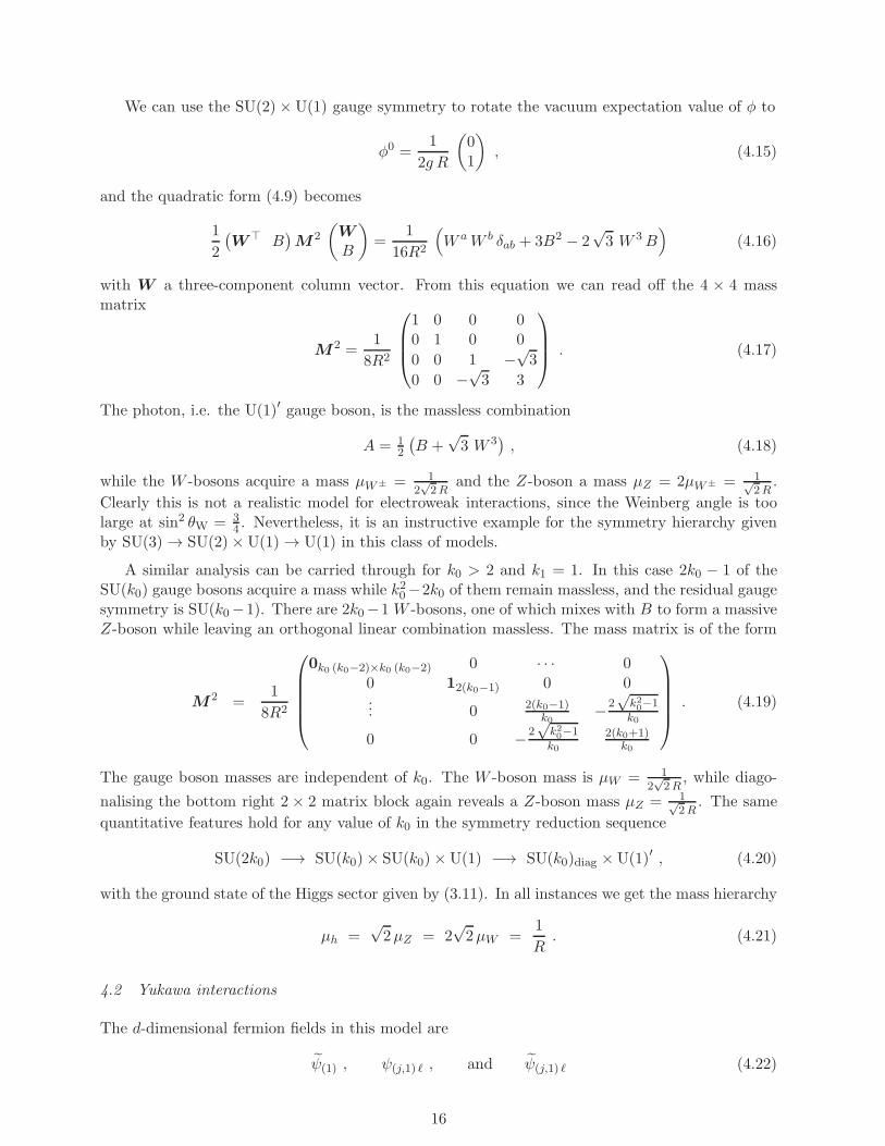
We can use the SU(2)×U(1) gauge symmetry to rotate the vacuum expectation value of φ to

φ0 =1

2g R

(01

), (4.15)

and the quadratic form (4.9) becomes

1

2

(W⊤ B

)M2

(W

B

)=

1

16R2

(W aW b δab + 3B2 − 2

√3 W 3B

)(4.16)

with W a three-component column vector. From this equation we can read off the 4 × 4 massmatrix

M2 =1

8R2

1 0 0 00 1 0 0

0 0 1 −√3

0 0 −√3 3

. (4.17)

The photon, i.e. the U(1)′ gauge boson, is the massless combination

A = 12

(B +

√3 W 3

), (4.18)

while the W -bosons acquire a mass µW± = 12√2R

and the Z-boson a mass µZ = 2µW± = 1√2R

.

Clearly this is not a realistic model for electroweak interactions, since the Weinberg angle is toolarge at sin2 θW = 3

4 . Nevertheless, it is an instructive example for the symmetry hierarchy givenby SU(3) → SU(2)×U(1) → U(1) in this class of models.

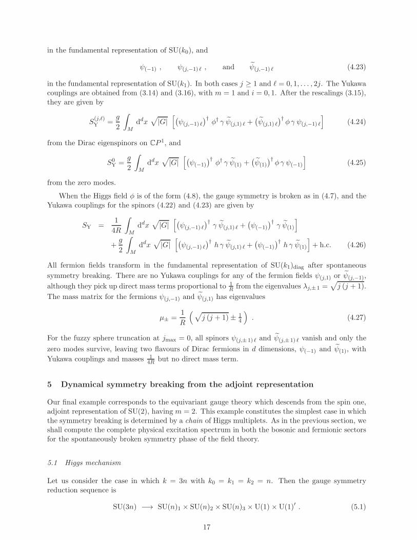
A similar analysis can be carried through for k0 > 2 and k1 = 1. In this case 2k0 − 1 of theSU(k0) gauge bosons acquire a mass while k20−2k0 of them remain massless, and the residual gaugesymmetry is SU(k0−1). There are 2k0−1W -bosons, one of which mixes with B to form a massiveZ-boson while leaving an orthogonal linear combination massless. The mass matrix is of the form

M2 =1

8R2

0k0 (k0−2)×k0 (k0−2) 0 · · · 0

0 12(k0−1) 0 0... 0 2(k0−1)

k0−2

√k20−1

k0

0 0 −2√

k20−1

k0

2(k0+1)k0

. (4.19)

The gauge boson masses are independent of k0. The W -boson mass is µW = 12√2R

, while diago-

nalising the bottom right 2× 2 matrix block again reveals a Z-boson mass µZ = 1√2R

. The same

quantitative features hold for any value of k0 in the symmetry reduction sequence

SU(2k0) −→ SU(k0)× SU(k0)×U(1) −→ SU(k0)diag ×U(1)′ , (4.20)

with the ground state of the Higgs sector given by (3.11). In all instances we get the mass hierarchy

µh =√2µZ = 2

√2µW =

1

R. (4.21)

4.2 Yukawa interactions

The d-dimensional fermion fields in this model are

ψ(1) , ψ(j,1) ℓ , and ψ(j,1) ℓ (4.22)

16

in the fundamental representation of SU(k0), and

ψ(−1) , ψ(j,−1) ℓ , and ψ(j,−1) ℓ (4.23)

in the fundamental representation of SU(k1). In both cases j ≥ 1 and ℓ = 0, 1, . . . , 2j. The Yukawacouplings are obtained from (3.14) and (3.16), with m = 1 and i = 0, 1. After the rescalings (3.15),they are given by

S(j,ℓ)Y =

g

2

∫

Mddx

√|G|

[(ψ(j,−1) ℓ

)†φ† γ ψ(j,1) ℓ +

(ψ(j,1) ℓ

)†φγ ψ(j,−1) ℓ

](4.24)

from the Dirac eigenspinors on CP 1, and

S0Y =

g

2

∫

Mddx

√|G|

[(ψ(−1)

)†φ† γ ψ(1) +

(ψ(1)

)†φγ ψ(−1)

](4.25)

from the zero modes.

When the Higgs field φ is of the form (4.8), the gauge symmetry is broken as in (4.7), and theYukawa couplings for the spinors (4.22) and (4.23) are given by

SY =1

4R

∫

Mddx

√|G|

[(ψ(j,−1) ℓ

)†γ ψ(j,1) ℓ +

(ψ(−1)

)†γ ψ(1)

]

+g

2

∫

Mddx

√|G|

[(ψ(j,−1) ℓ

)†hγ ψ(j,1) ℓ +

(ψ(−1)

)†hγ ψ(1)

]+ h.c. (4.26)

All fermion fields transform in the fundamental representation of SU(k1)diag after spontaneous

symmetry breaking. There are no Yukawa couplings for any of the fermion fields ψ(j,1) or ψ(j,−1),

although they pick up direct mass terms proportional to 1R from the eigenvalues λj,± 1 =

√j (j + 1).

The mass matrix for the fermions ψ(j,−1) and ψ(j,1) has eigenvalues

µ± =1

R

(√j (j + 1)± 1

4

). (4.27)

For the fuzzy sphere truncation at jmax = 0, all spinors ψ(j,± 1) ℓ and ψ(j,± 1) ℓ vanish and only the

zero modes survive, leaving two flavours of Dirac fermions in d dimensions, ψ(−1) and ψ(1), with

Yukawa couplings and masses 14R but no direct mass term.

5 Dynamical symmetry breaking from the adjoint representation

Our final example corresponds to the equivariant gauge theory which descends from the spin one,adjoint representation of SU(2), having m = 2. This example constitutes the simplest case in whichthe symmetry breaking is determined by a chain of Higgs multiplets. As in the previous section, weshall compute the complete physical excitation spectrum in both the bosonic and fermionic sectorsfor the spontaneously broken symmetry phase of the field theory.

5.1 Higgs mechanism

Let us consider the case in which k = 3n with k0 = k1 = k2 = n. Then the gauge symmetryreduction sequence is

SU(3n) −→ SU(n)1 × SU(n)2 × SU(n)3 ×U(1) ×U(1)′ . (5.1)

17

There are two complex n×n matrices of Higgs fields φ1, with SU(n)1 acting on the left and SU(n)2acting on the right, and φ2, with SU(n)2 acting on the left and SU(n)3 on the right. The U(1)and U(1)′ generators can be taken to be any two linearly independent generators of SU(3n) whichcommute with all three SU(n) factors. In particular, we can take

Y =1√n

1 0 0

0 −1 0

0 0 0

and Y ′ =

1√n

0 0 0

0 1 0

0 0 −1

, (5.2)

where each entry is an n× n matrix. With this normalisation the scalar field φ1 has Y -charge 2√n

and Y ′-charge − 1√n, while φ2 has Y -charge − 1√

nand Y ′-charge 2√

n.

The Higgs potential (3.7) is

V (φ1, φ2) =n

4g2R4− 1

2R2tr(φ†1 φ1 + φ†2 φ2

)+g2 tr

((φ†1 φ1

)2 −(φ†1 φ1 φ

†2 φ2

)+(φ†2 φ2

)2). (5.3)

The general solution (3.11) in this case, with ζ1 = ζ2 = 1, gives the vacuum configuration

φ01 = φ02 =1√2 g R

1n . (5.4)

This expectation value is invariant under a single copy of SU(n), which is a linear combinationof SU(n)1, SU(n)2 and SU(n)3. There is no linear combination of U(1) and U(1)′ that leaves itinvariant, so the gauge symmetry is reduced as

SU(3n) −→ SU(n)1 × SU(n)2 × SU(n)3 ×U(1) ×U(1)′ −→ SU(n) . (5.5)

In this case 2n2 gauge bosons acquire a mass and, of the 4n2 degrees of freedom in φ1 and φ2, atotal of 2n2 remain as physical Higgs fields. Expanding around the ground state, the latter fieldscan be represented by n× n hermitean matrices h1 and h2 with

φ1 =1√2 g R

1n + h1 and φ2 =1√2 g R

1n + h2 . (5.6)

Putting this form into (5.3) and examining the terms quadratic in h1 and h2, we find a 2× 2 massmatrix with Higgs masses given by the eigenvalues

µh> =

√3

Rand µh< =

1

R. (5.7)

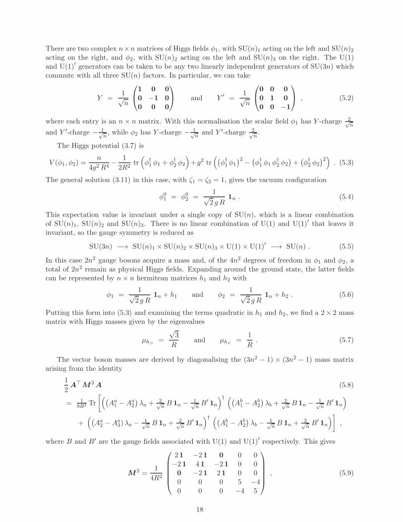
The vector boson masses are derived by diagonalising the (3n2 − 1) × (3n2 − 1) mass matrixarising from the identity

1

2A⊤M2 A (5.8)

= 18R2 Tr

[((Aa

1 −Aa2

)λa +

2√nB 1n − 1√

nB′

1n

)† ((Ab

1 −Ab2

)λb +

2√nB 1n − 1√

nB′

1n

)

+((Aa

2 −Aa3)λa − 1√

nB 1n + 2√

nB′

1n

)† ((Ab

1 −Ab2

)λb − 1√

nB 1n + 2√

nB′

1n

)],

where B and B′ are the gauge fields associated with U(1) and U(1)′ respectively. This gives

M2 =1

4R2

21 −21 0 0 0−21 41 −21 0 00 −21 21 0 00 0 0 5 −40 0 0 −4 5

, (5.9)

18

where each bold-face matrix block is of dimension (n2 − 1) × (n2 − 1). The massless SU(n) gaugebosons are

Aa = 1√3

(Aa

1 +Aa2 +Aa

3

), (5.10)

while the vector bosons W a = 1√2(Aa

1 −Aa3) acquire a mass

µW =1√2R

(5.11)

and V a = 1√6(Aa

1 − 2Aa2 +Aa

3) have mass

µV =

√3

2

1

R. (5.12)

The U(1) vector bosons mix as

Z = 1√2

(B +B′ ) and Z ′ = 1√

2

(B −B′ ) , (5.13)

with masses

µZ =1

2Rand µZ′ =

3

2

1

R. (5.14)

5.2 Yukawa interactions

The d-dimensional fermion fields in this model are

ψ(2) , ψ(j,2) ℓ , and ψ(j,2) ℓ with j ≥ 32 (5.15)

in the fundamental representation of SU(n)1, together with

ψ(j,0) ℓ and ψ(j,0) ℓ with j ≥ 12 (5.16)

in the fundamental representation of SU(n)2, and

ψ(−2) , ψ(j,−2) ℓ , and ψ(j,−2) ℓ with j ≥ 32 (5.17)

in the fundamental representation of SU(n)3. In all cases ℓ = 0, 1, . . . , 2j. The Yukawa couplingsafter dimensional reduction are

SY =g

2

∫

Mddx

√|G|

[(ψ(j,2) ℓ

)†φ1 ψ(j,0) ℓ +

(ψ(j,0) ℓ

)†φ2 ψ(j,−2) ℓ

]+ h.c. , (5.18)

as the spinor fields ψ(−2), ψ(2), ψ(j,2) ℓ and ψ(j,−2) ℓ have no Yukawa couplings. The former two

fermions are massless, while the latter two fermions have direct mass terms proportional to 1R com-

ing from the eigenvalues λj,± 2 =√

(j − 12) (j +

32). All fermion fields transform in the fundamental

representation of SU(n) after spontaneous symmetry breaking. After substituting the Higgs fields(5.6) into (5.18), the Yukawa masses can be read off from the general formula (3.18) with pi = 0and |vi|2 = 1

2 .

19

6 Conclusions

In this paper we have explicitly worked out the SU(2)-equivariant dimensional reduction of puremassless Yang-Mills-Dirac theory over the coset space CP 1, including a systematic incorporationof Dirac monopole backgrounds. The internal magnetic fluxes induce a Higgs potential as well asYukawa couplings between the reduced fermion fields and the Higgs fields, with the standard formof dynamical symmetry breaking. In particular, in certain instances the zero modes of the Diracoperator on CP 1 acquire Yukawa interactions. In our formulation we are able to naturally induceboth massive and massless fermions, as well as a chiral gauge theory. When inducing massive Diracspinors associated to higher spinor harmonics on CP 1, it is more natural to use a fuzzy sphereCP 1

F for the internal space, as it provides an SU(2)-equivariant truncation of the infinite tower ofmodes and can also be used to truncate to the finitely-many flavours of massless symmetric spinormodes. We worked out several explicit examples of spontaneous symmetry breaking, includingclasses containing the standard electroweak symmetry breaking sequence as a special case and alsoa class involving a chain of Higgs fields. In all cases we explicitly worked out the complete physicalparticle spectrum in the dimensionally reduced field theory after dynamical symmetry breaking.

There are a few technical points which we have brushed over in our analysis. For example, wehave not analysed the stability of the Higgs vacua φ0i that led to dynamical symmetry breaking.Although the spectrum of fluctuations around the solutions we have used certainly do not containany unstable modes, because these vacua minimize the Higgs potential, one should check whetheror not there are any flat modes which may lead to a non-trivial vacuum moduli space. This appearsto be a rather non-trivial task even for the simplest Higgs vacua we have found. We have also notaddressed the problem of renormalizability of the dimensionally reduced field theory. Since theoriginal higher-dimensional Yang-Mills-Dirac theory is generically non-renormalizable, keeping allhigher modes in the lower-dimensional model generically leads to a non-renormalizable field theory.It is not clear if the truncations we have used can help to give better quantum behaviour. Itwould be interesting to analyse further if any symmetries of the coupled chain field system (e.g.supersymmetry) could lead to renormalizable quantum field theories after dimensional reduction.

In this article we have only focused on the simplest possible homogeneous space to elucidateas clearly as possible the effects of topologically non-trivial gauge field configurations obtained bygauging the holonomy group of the coset. In principle, one can consider more complicated cosetspaces G/H with the hope of obtaining more realistic physical theories resembling the standardmodel. As regards the fermionic sector, a particularly crucial role is played by those cosets whichadmit a finite-dimensional matrix approximation (G/H)F , such as the fuzzy complex projectivespaces CPN

F where an explicit universal Dirac operator is known and whose spectrum has beenstudied in detail in [22]. For N = 2, the SU(3)-equivariant dimensional reduction of Yang-Millstheory over CP 2 has been carried out in detail in [14] incorporating both SU(2) instanton and U(1)monopole backgrounds associated with the holonomy group U(3) of CP 2. It would be interesting toextend the techniques of this paper to these classes of equivariant dimensional reduction schemes.In particular, one can compare with results of [6] where the use of (fuzzy) complex projectiveplanes has been suggested as a natural internal space for Kaluza-Klein reduction, leading to theappropriate chiral fermionic spectrum of the standard model.

It would also be interesting to use our techniques to study the reductions of the ten-dimensionalN = 1 supersymmetric E8 gauge theories over six-dimensional coset spaces considered in [2, 3],although many of these cosets have no known fuzzy versions. Nevertheless, the SU(3) equiv-ariant dimensional reduction of Yang-Mills theory over the six-dimensional non-symmetric spaceSU(3)

/U(1)2 is explicitly worked out in [14] including U(1) monopole backgrounds associated with

the maximal torus U(1) × U(1) of SU(3). An outline of a scheme that could allow for a fuzzyversion of this coset space was proposed in [23]. It would be interesting to compare the resulting

20

four-dimensional field theories with those of [3], particularly the supersymmetry properties whicharise under equivariant dimensional reduction. Our reduction techniques could also be applied inprinciple to the superstring theories on nearly Kahler backgrounds considered in [4]. In this regardit would be interesting to find a natural interpretation for the internal fluxes within the context ofthese superstring models, along the lines of the flux stabilization mechanisms on arrays of D-branesin Type II string theory suggested in [8, 11, 12, 14].

Acknowledgments

B.P.D. wishes to thank the Dublin Institute of Advanced Studies for financial support. The workof R.J.S. was supported in part by the EU-RTN Network Grant MRTN-CT-2004-005104.

References

[1] P. Forgacs and N.S. Manton, Commun. Math. Phys. 72 (1980) 15; C.H. Taubes, Commun.Math. Phys. 75 (1980) 207.

[2] D. Kapetanakis and G. Zoupanos, Phys. Rept. 219 (1992) 1.

[3] P. Manousselis and G. Zoupanos, JHEP 03 (2002) 002 [arXiv:hep-ph/0111125]; JHEP 11

(2004) 025 [arXiv:hep-ph/0406207]; A. Chatzistavrakidis, P. Manousselis, N. Prezas andG. Zoupanos, Phys. Lett. B 656 (2007) 152 [arXiv:0708.3222 [hep-th]]; G. Douzas, T. Gram-matikopoulos and G. Zoupanos, arXiv:0808.3236 [hep-th].

[4] G. Lopes Cardoso, G. Curio, G. Dall’Agata, D. Lust, P. Manousselis and G. Zoupanos, Nucl.Phys. B 652 (2003) 5 [arXiv:hep-th/0211118]; P. Manousselis, N. Prezas and G. Zoupanos,Nucl. Phys. B 739 (2006) 85 [arXiv:hep-th/0511122]; A. Chatzistavrakidis, P. Manousselis andG. Zoupanos, arXiv:0811.2182 [hep-th].

[5] E. Witten, in: Proceedings of the 1983 Shelter Island Conference on Quantum Field Theory

and the Fundamental Problems of Physics, eds. R. Jackiw, N.N. Khuri, S. Weinberg andE. Witten (MIT Press, 1985).

[6] B.P. Dolan and C. Nash, JHEP 10 (2002) 041 [arXiv:hep-th/0207078]; JHEP 07 (2002) 057[arXiv:hep-th/0207007].

[7] L. Alvarez-Consul and O. Garcıa-Prada, J. Reine Angew. Math. 556 (2003) 1[arXiv:math.DG/0112160]; Commun. Math. Phys. 238 (2003) 1 [arXiv:math.DG/0112161].

[8] O. Lechtenfeld, A.D. Popov and R.J. Szabo, Progr. Theor. Phys. Suppl. 171 (2007) 258[arXiv:0706.0979 [hep-th]].

[9] O. Garcıa-Prada, Commun. Math. Phys. 156 (1993) 527; Int. J. Math. 5 (1994) 1.

[10] L. Alvarez-Consul and O. Garcıa-Prada, Int. J. Math. 12 (2001) 159.

[11] O. Lechtenfeld, A.D. Popov and R.J. Szabo, JHEP 12 (2003) 022 [arXiv:hep-th/0310267];JHEP 09 (2006) 054 [arXiv:hep-th/0603232].

[12] A.D. Popov and R.J. Szabo, J. Math. Phys. 47 (2006) 012306 [arXiv:hep-th/0504025].

[13] A.D. Popov, arXiv:0712.1756 [hep-th]; Lett. Math. Phys. 84 (2008) 139 [arXiv:0801.0808 [hep-th]].

21

[14] O. Lechtenfeld, A.D. Popov and R.J. Szabo, JHEP 08 (2008) 093 [arXiv:0806.2791 [hep-th]].

[15] A.D. Popov, Phys. Rev. D 77 (2008) 125026 [arXiv:0803.3320 [hep-th]]; arXiv:0804.3845 [hep-th].

[16] G.B. Segal, Publ. Math. IHES (Paris) 34 (1968) 113; 129.

[17] M. Cahen, A. Franc and S. Gutt, Lett. Math. Phys. 32 (1994) 365; C. Bar, Analysis 6 (1996)899.

[18] J. Madore, Class. Quant. Grav. 9 (1992) 69.

[19] P. Aschieri, J. Madore, P. Manousselis and G. Zoupanos, JHEP 04 (2004) 034 [arXiv:hep-th/0310072].

[20] P. Aschieri, T. Grammatikopoulos, H. Steinacker and G. Zoupanos, JHEP 09 (2006) 026[arXiv:hep-th/0606021]; H. Steinacker and G. Zoupanos, JHEP 09 (2007) 017 [arXiv:0706.0398[hep-th]].

[21] H. Grosse and P. Presnajder, Lett. Math. Phys. 33 (1995) 171; H. Grosse, C. Klimcik andP. Presnajder, Commun. Math. Phys. 178 (1996) 507 [arXiv:hep-th/9510083]; U. Carow-Watamura and S. Watamura, Commun. Math. Phys. 183 (1997) 365 [arXiv:hep-th/9605003].

[22] B.P. Dolan, I. Huet, S. Murray and D. O’Connor, JHEP 03 (2008) 029 [arXiv:0711.1347 [hep-th]].

[23] C. Samann, JHEP 02 (2008) 111 [arXiv:hep-th/0612173].

22