Dimensional Characteristics of theNon-wandering Sets of Open Billiards

Paul Wright, BSc. (Honours)

2014

This thesis is presented for the degree ofDoctor of Philosophy of The University ofWestern Australia School of Mathematics

and Statistics.

Abstract

An open billiard is a dynamical system in which a pointlike particle moves at constant speedin an unbounded domain, reflecting off a boundary according to the classical laws of optics.This thesis is an investigation of dimensional characteristics of the non-wandering set ofan open billiard in the exterior of three or more strictly convex bodies satisfying Ikawa’sno-eclipse condition. The billiard map for these systems is an axiom A diffeomorphismwith a finite Markov partition. The non-wandering set is a hyperbolic set with stableand unstable manifolds satisfying a certain reflection property. The characteristics weinvestigate include the topological and measure-theoretic entropy, topological pressure,Lyapunov exponents, lower and upper box dimension and the Hausdorff dimension of thenon-wandering set. In particular, we investigate the dependence of Hausdorff dimension ondeformations to the boundary of the billiard obstacles. While the dependence of dimensionalcharacteristics on perturbations of a system has been studied before, this is the first timethis question has been answered for dynamical billiards.

We find upper and lower bounds for the Hausdorff dimension using two different methods:one involving bounding the size of curves on convex fronts and the other using Bowen’sequation and the variational principle for topological pressure. Both methods lead to thesame upper and lower bounds. In the first method, we use a well known recurrence relationfor the successive curvatures of convex fronts to find bounds on the size of the fronts.This allows us to construct Lipschitz (but not bi-Lipszhitz) homeomorphisms between thenon-wandering set and the one-sided symbol space. From there we obtain estimates ofthe dimension. This method has been previously used for open billiards in the plane. Weextend it to higher dimensions and make improvements to the results in the plane.

The second method is a more general approach from the dimension theory of dynamicalsystems. In the plane, the billiard map is conformal, meaning that its derivative is amultiple of an isometry. For conformal maps, the Hausdorff dimension of non-wanderingsets is well-understood and satisfies Bowen’s equation. In higher dimensions, the billiardmap is not conformal and the dimension only satisfies some estimates.

We consider what happens to the non-wandering set when one or more obstacles in abilliard are deformed or shifted differentiably. In two and higher dimensions, we show thatall points in the non-wandering set depend smoothly on deformations to the boundary. Weuse a well-known lemma about the position of periodic points in a non-eclipsing billiard,and differentiate these points to get a cyclic tridiagonal system of equations. For billiards in

i

Abstract

the plane, we use Bowen’s equation to further show that the Hausdorff dimension dependssmoothly on the deformations, and we find an upper bound for the derivative of thedimension with respect to the deformation parameter. For higher dimensions, there is noexact equation to differentiate because the billiard ball map is non-conformal.

We obtain some new results for non-conformal hyperbolic dynamics. The concept of anaverage conformal repeller was developed as a generalisation of a conformal repeller. Weextend this idea by generalizing conformal hyperbolic sets to average conformal hyperbolicsets. A hyperbolic set is average conformal if it has only two distinct Lyapunov exponents,one positive and one negative. We obtain an equation for the Hausdorff dimension of anaverage conformal hyperbolic set. While we know that a billiard in three or more dimensionsis never conformal, it is unknown whether there exist billiards that are average conformal.

Finally, we consider several examples of billiards with deformations and apply thetechniques developed in this thesis to obtain numerical upper and lower bounds for theHausdorff dimension and its derivative.

ii

Acknowledgements

To my supervisor, Professor Luchezar Stoyanov, thank you for years of mentoring, advice,editing and support.

Thanks to the University of Western Australia for providing me with this incredibleexperience. I was assisted throughout my PhD by the following scholarships:

• Australian Postgraduate Award,• Bruce and Betty Green Post Graduate Scholarship,• UWA Safety Net Top up Scholarship,• UWA Travel Grant,• PhD Completion Scholarship.

Thank you to the hosts and speakers of the Limit Theorems in Dynamical Systems eventin Lausanne, and to the Centre Interfacultaire Bernoulli.

Thank you to my co-supervisor Winthrop Professor Lyle Noakes, and to all the staff at theUWA mathematics department.

To all my friends, including Andre Rhine-Davis, Andrew Cann, James Hales, Tarryn Rae,Shreya Bhattarai, Brian Corr, Maya Kerr and Richard Greenhalgh: Thanks for varioushelpful comments, suggestions and letting me bounce ideas off your C3-smooth, strictlyconvex foreheads.

Thanks to Anthony Di Pietro for extensive help with editing and LATEX.

To Kitty Byrne, who was somehow able to find mistakes in my thesis by pointing to arandom spot on the page, thanks for your love and encouragement.

To Madge Carew-Hopkins, there’s no specific thing I can thank you for because you doeverything for me. Thank you for our life together.

To my brother Mark, thanks for keeping me grounded, and to all of my extended family,

iii

Acknowledgements

thank you for your genuine interest and encouragement.

In addition to their love and support, my parents Deidre and Ricky have been amazinglisteners, to the point that I can explain not just the central ideas of my thesis but sometimesthe fine details. Thank you.

iv

Contents

Abstract i

Acknowledgements iii

Contents v

List of Figures x

1 Introduction 11.1 History of dynamical billiards . . . . . . . . . . . . . . . . . . . . . . . . . 11.2 Dimension theory of dynamical systems . . . . . . . . . . . . . . . . . . . 21.3 Outline and main results . . . . . . . . . . . . . . . . . . . . . . . . . . . . 3

1.3.1 Chapter 2 — Preliminaries . . . . . . . . . . . . . . . . . . . . . . 31.3.2 Chapter 3 — Open billiards . . . . . . . . . . . . . . . . . . . . . . 31.3.3 Chapter 4 — Dimension theory in dynamical systems . . . . . . . 41.3.4 Chapter 5 — Estimates of Hausdorff dimension of the non-wandering

set . . . . . . . . . . . . . . . . . . . . . . . . . . . . . . . . . . . . 41.3.5 Chapter 6 — Differentiability of Hausdorff dimension for planar

billiards . . . . . . . . . . . . . . . . . . . . . . . . . . . . . . . . . 51.3.6 Chapter 7 — Differentiability of Hausdorff dimension for nonplanar

billiards . . . . . . . . . . . . . . . . . . . . . . . . . . . . . . . . . 51.3.7 Chapter 8 — Average conformal hyperbolic sets . . . . . . . . . . . 61.3.8 Chapter 9 — Examples and further research . . . . . . . . . . . . . 6

2 Preliminaries 72.1 Notation . . . . . . . . . . . . . . . . . . . . . . . . . . . . . . . . . . . . . 72.2 Real analysis . . . . . . . . . . . . . . . . . . . . . . . . . . . . . . . . . . 8

2.2.1 Hölder and Lipschitz functions . . . . . . . . . . . . . . . . . . . . 82.2.2 Differentiability classes for multiple variables . . . . . . . . . . . . 82.2.3 Cf notation . . . . . . . . . . . . . . . . . . . . . . . . . . . . . . . 92.2.4 Implicit function theorem . . . . . . . . . . . . . . . . . . . . . . . 92.2.5 Uniformly convergent sequences . . . . . . . . . . . . . . . . . . . . 10

2.3 Differential geometry . . . . . . . . . . . . . . . . . . . . . . . . . . . . . . 10

v

Contents

2.3.1 Curvature of plane curves . . . . . . . . . . . . . . . . . . . . . . . 102.3.2 Curvature of higher dimensional surfaces . . . . . . . . . . . . . . . 102.3.3 Orthonormal parametrization . . . . . . . . . . . . . . . . . . . . . 11

2.4 Matrices . . . . . . . . . . . . . . . . . . . . . . . . . . . . . . . . . . . . . 122.4.1 Block matrices . . . . . . . . . . . . . . . . . . . . . . . . . . . . . 122.4.2 Matrix norms and block norms . . . . . . . . . . . . . . . . . . . . 122.4.3 Some types of matrices . . . . . . . . . . . . . . . . . . . . . . . . . 132.4.4 Varah’s theorem and extensions . . . . . . . . . . . . . . . . . . . . 14

3 Open billiards 173.1 Billiards . . . . . . . . . . . . . . . . . . . . . . . . . . . . . . . . . . . . . 17

3.1.1 The billiard ball map . . . . . . . . . . . . . . . . . . . . . . . . . . 193.1.2 Non-wandering set . . . . . . . . . . . . . . . . . . . . . . . . . . . 193.1.3 The phase space of the billiard as a Riemannian manifold . . . . . 20

3.2 Parametrization . . . . . . . . . . . . . . . . . . . . . . . . . . . . . . . . . 203.2.1 Curvature . . . . . . . . . . . . . . . . . . . . . . . . . . . . . . . . 213.2.2 Planar billiards . . . . . . . . . . . . . . . . . . . . . . . . . . . . . 22

3.3 Periodic points . . . . . . . . . . . . . . . . . . . . . . . . . . . . . . . . . 223.3.1 Length function . . . . . . . . . . . . . . . . . . . . . . . . . . . . . 22

3.4 Symbolic dynamics . . . . . . . . . . . . . . . . . . . . . . . . . . . . . . . 233.5 Relaxing conditions . . . . . . . . . . . . . . . . . . . . . . . . . . . . . . . 253.6 Billiard constants . . . . . . . . . . . . . . . . . . . . . . . . . . . . . . . . 26

3.6.1 Distances . . . . . . . . . . . . . . . . . . . . . . . . . . . . . . . . 273.6.2 Curvatures . . . . . . . . . . . . . . . . . . . . . . . . . . . . . . . 273.6.3 Collision angles . . . . . . . . . . . . . . . . . . . . . . . . . . . . . 273.6.4 Estimating billiard constants . . . . . . . . . . . . . . . . . . . . . 28

4 Dimension theory in dynamical systems 294.1 Introduction . . . . . . . . . . . . . . . . . . . . . . . . . . . . . . . . . . . 294.2 Fractal dimensions . . . . . . . . . . . . . . . . . . . . . . . . . . . . . . . 29

4.2.1 Hausdorff dimension . . . . . . . . . . . . . . . . . . . . . . . . . . 294.2.2 Box dimension . . . . . . . . . . . . . . . . . . . . . . . . . . . . . 304.2.3 Packing dimension . . . . . . . . . . . . . . . . . . . . . . . . . . . 30

4.3 Invariant and non-wandering sets, expanding and expansive maps . . . . . 314.3.1 Repellers . . . . . . . . . . . . . . . . . . . . . . . . . . . . . . . . 31

4.4 Hyperbolic diffeomorphisms . . . . . . . . . . . . . . . . . . . . . . . . . . 314.4.1 Hyperbolic flows . . . . . . . . . . . . . . . . . . . . . . . . . . . . 324.4.2 Stable and unstable manifolds . . . . . . . . . . . . . . . . . . . . . 334.4.3 Local product structure and Markov partitions . . . . . . . . . . . 344.4.4 Coding diffeomorphisms using a symbol space . . . . . . . . . . . . 35

4.5 Non-conformal hyperbolic sets . . . . . . . . . . . . . . . . . . . . . . . . . 36

vi

Contents

4.5.1 Measures . . . . . . . . . . . . . . . . . . . . . . . . . . . . . . . . 364.5.2 Lyapunov exponents . . . . . . . . . . . . . . . . . . . . . . . . . . 364.5.3 Continuity of foliations and the local product map . . . . . . . . . 37

4.6 Entropy and pressure . . . . . . . . . . . . . . . . . . . . . . . . . . . . . . 384.6.1 Entropy of a partition . . . . . . . . . . . . . . . . . . . . . . . . . 394.6.2 Classical topological pressure of a function via separated sets . . . 394.6.3 Dimensional definition of pressure of a function . . . . . . . . . . . 404.6.4 Measure theoretic pressure and entropy . . . . . . . . . . . . . . . 404.6.5 Barreira’s pressure for function sequences with respect to finite

open covers . . . . . . . . . . . . . . . . . . . . . . . . . . . . . . . 414.6.6 Pressure of subadditive and super-additive sequences via separated

sets . . . . . . . . . . . . . . . . . . . . . . . . . . . . . . . . . . . 414.6.7 Pressure on the symbol space . . . . . . . . . . . . . . . . . . . . . 424.6.8 Equivalence of definitions for pressure . . . . . . . . . . . . . . . . 434.6.9 Variational principle . . . . . . . . . . . . . . . . . . . . . . . . . . 44

4.7 Dimension theory in conformal hyperbolic dynamics . . . . . . . . . . . . 444.7.1 Bowen’s equation . . . . . . . . . . . . . . . . . . . . . . . . . . . . 444.7.2 Dimension of the locally maximal hyperbolic set of a conformal map 45

4.8 Dimension theory in non-conformal hyperbolic dynamics . . . . . . . . . . 454.9 Conformality of the billiard ball map . . . . . . . . . . . . . . . . . . . . . 47

5 Estimates of Hausdorff dimension of the non-wandering set 495.1 Introduction . . . . . . . . . . . . . . . . . . . . . . . . . . . . . . . . . . . 495.2 Main Theorem . . . . . . . . . . . . . . . . . . . . . . . . . . . . . . . . . 495.3 Convex fronts . . . . . . . . . . . . . . . . . . . . . . . . . . . . . . . . . . 505.4 Coding M0 and X0 . . . . . . . . . . . . . . . . . . . . . . . . . . . . . . . 51

5.4.1 Evolution of Fronts . . . . . . . . . . . . . . . . . . . . . . . . . . . 515.4.2 Estimating Θ . . . . . . . . . . . . . . . . . . . . . . . . . . . . . . 525.4.3 Curves on convex fronts . . . . . . . . . . . . . . . . . . . . . . . . 53

5.5 Estimating kj for large j . . . . . . . . . . . . . . . . . . . . . . . . . . . . 545.5.1 Estimating δj(s) . . . . . . . . . . . . . . . . . . . . . . . . . . . . 55

5.6 Hausdorff dimension of X0 . . . . . . . . . . . . . . . . . . . . . . . . . . . 565.6.1 Representation map . . . . . . . . . . . . . . . . . . . . . . . . . . 57

5.7 Hausdorff dimension of M0 . . . . . . . . . . . . . . . . . . . . . . . . . . 585.8 Dimension product structure . . . . . . . . . . . . . . . . . . . . . . . . . 595.9 Calculating the Hölder constant . . . . . . . . . . . . . . . . . . . . . . . . 595.10 Domain of g(γ, d) . . . . . . . . . . . . . . . . . . . . . . . . . . . . . . . . 60

6 Differentiability of Hausdorff dimension for planar billiards 636.1 Introduction . . . . . . . . . . . . . . . . . . . . . . . . . . . . . . . . . . . 63

6.1.1 Example . . . . . . . . . . . . . . . . . . . . . . . . . . . . . . . . . 64

vii

Contents

6.2 Billiard deformations . . . . . . . . . . . . . . . . . . . . . . . . . . . . . . 646.2.1 Shift maps and billiard expansions . . . . . . . . . . . . . . . . . . 66

6.3 Derivatives of parameters . . . . . . . . . . . . . . . . . . . . . . . . . . . 666.3.1 Estimating − ∂

∂α∇G . . . . . . . . . . . . . . . . . . . . . . . . . . 686.3.2 The Hessian Matrix . . . . . . . . . . . . . . . . . . . . . . . . . . 69

6.4 Solving the cyclic tridiagonal system . . . . . . . . . . . . . . . . . . . . . 706.4.1 Estimating the Euclidean norm of y . . . . . . . . . . . . . . . . . 716.4.2 Calculating the inverse . . . . . . . . . . . . . . . . . . . . . . . . . 716.4.3 Varah’s Theorem . . . . . . . . . . . . . . . . . . . . . . . . . . . . 71

6.5 Higher derivatives of parameters . . . . . . . . . . . . . . . . . . . . . . . 736.6 Extension to aperiodic trajectories . . . . . . . . . . . . . . . . . . . . . . 736.7 Derivatives of other billiard properties . . . . . . . . . . . . . . . . . . . . 75

6.7.1 Estimating derivatives of distances, curvatures and collision angles 756.7.2 Stable and unstable manifolds . . . . . . . . . . . . . . . . . . . . . 766.7.3 Curvature of unstable manifolds . . . . . . . . . . . . . . . . . . . 776.7.4 Bounds on Hausdorff dimension . . . . . . . . . . . . . . . . . . . . 78

6.8 Derivative of Hausdorff dimension . . . . . . . . . . . . . . . . . . . . . . . 80

7 Differentiability of Hausdorff dimension for nonplanar billiards 857.1 Introduction . . . . . . . . . . . . . . . . . . . . . . . . . . . . . . . . . . . 85

7.1.1 Notation . . . . . . . . . . . . . . . . . . . . . . . . . . . . . . . . . 857.2 Billiard deformations in higher dimensions . . . . . . . . . . . . . . . . . . 857.3 Derivatives of parameters . . . . . . . . . . . . . . . . . . . . . . . . . . . 86

7.3.1 Calculating − ∂∂α∇G . . . . . . . . . . . . . . . . . . . . . . . . . . 88

7.3.2 Hessian matrix . . . . . . . . . . . . . . . . . . . . . . . . . . . . . 897.4 System of matrix equations . . . . . . . . . . . . . . . . . . . . . . . . . . 907.5 Higher derivatives of parameters . . . . . . . . . . . . . . . . . . . . . . . 927.6 Extension to aperiodic trajectories . . . . . . . . . . . . . . . . . . . . . . 937.7 Derivatives of distances, curvatures, collision angles and convex fronts . . 94

7.7.1 Estimating derivatives of distances, curvatures and collision angles 947.7.2 Unstable manifolds and convex fronts . . . . . . . . . . . . . . . . 957.7.3 Curvature of unstable manifolds . . . . . . . . . . . . . . . . . . . 96

7.8 Hausdorff dimension of the non-wandering set . . . . . . . . . . . . . . . . 987.8.1 Bounds on Hausdorff dimension . . . . . . . . . . . . . . . . . . . . 99

7.9 Future approaches to solving the problem . . . . . . . . . . . . . . . . . . 997.9.1 Average conformal billiards . . . . . . . . . . . . . . . . . . . . . . 997.9.2 Exact equations for Hausdorff dimensions of non-conformal re-

pellers or hyperbolic sets . . . . . . . . . . . . . . . . . . . . . . . . 100

8 Average conformal hyperbolic sets 1018.1 Introduction . . . . . . . . . . . . . . . . . . . . . . . . . . . . . . . . . . . 101

viii

Contents

8.2 Preliminaries . . . . . . . . . . . . . . . . . . . . . . . . . . . . . . . . . . 1028.2.1 Conformal, weakly conformal, quasi-conformal, and average con-

formal maps . . . . . . . . . . . . . . . . . . . . . . . . . . . . . . . 1038.2.2 Sub-additive and super-additive sequences . . . . . . . . . . . . . . 105

8.3 Theorems for average conformal hyperbolic sets . . . . . . . . . . . . . . . 1088.3.1 Variational principle . . . . . . . . . . . . . . . . . . . . . . . . . . 109

8.4 Lemmas for the main theorem . . . . . . . . . . . . . . . . . . . . . . . . . 1108.4.1 Summary of lemmas . . . . . . . . . . . . . . . . . . . . . . . . . . 113

8.5 Proof of main theorem . . . . . . . . . . . . . . . . . . . . . . . . . . . . . 1138.6 Further results . . . . . . . . . . . . . . . . . . . . . . . . . . . . . . . . . 116

8.6.1 Local product structure . . . . . . . . . . . . . . . . . . . . . . . . 1168.6.2 Are billiards ever average conformal? . . . . . . . . . . . . . . . . . 117

9 Examples and further research 1199.1 Remarks . . . . . . . . . . . . . . . . . . . . . . . . . . . . . . . . . . . . . 119

9.1.1 Non-wandering sets with Hausdorff dimension close to the topo-logical dimension . . . . . . . . . . . . . . . . . . . . . . . . . . . . 119

9.1.2 The map between non-wandering sets of different billiards . . . . . 1209.2 Examples . . . . . . . . . . . . . . . . . . . . . . . . . . . . . . . . . . . . 121

9.2.1 Billiard obstacles that are not disks . . . . . . . . . . . . . . . . . . 1219.2.2 Tetrahedron billiard . . . . . . . . . . . . . . . . . . . . . . . . . . 1229.2.3 Isosceles billiard deformation . . . . . . . . . . . . . . . . . . . . . 123

9.3 Questions for future research . . . . . . . . . . . . . . . . . . . . . . . . . 1249.4 Investigating billiards with Mathematica . . . . . . . . . . . . . . . . . . . 125

9.4.1 Notebook 1: Non-wandering set . . . . . . . . . . . . . . . . . . . . 1259.4.2 Notebook 2: Estimating dimension . . . . . . . . . . . . . . . . . . 1259.4.3 Notebook 3: Estimating dimension for unit spheres . . . . . . . . . 1269.4.4 Notebook 4: Derivatives of dimension for planar billiard deforma-

tions with moving unit disks . . . . . . . . . . . . . . . . . . . . . 1269.5 Examples . . . . . . . . . . . . . . . . . . . . . . . . . . . . . . . . . . . . 126

9.5.1 Examples from Notebook 1: two dimensions . . . . . . . . . . . . . 1279.5.2 Examples from Notebook 1: three dimensions . . . . . . . . . . . . 1289.5.3 Examples from Notebook 2 . . . . . . . . . . . . . . . . . . . . . . 1319.5.4 Examples from Notebook 3 . . . . . . . . . . . . . . . . . . . . . . 1339.5.5 Examples from Notebook 4 . . . . . . . . . . . . . . . . . . . . . . 135

A Inverse of a cyclic tridiagonal matrix 137

Bibliography 141

ix

List of Figures

1.1 Non-wandering sets . . . . . . . . . . . . . . . . . . . . . . . . . . . . . . . . . 21.2 Mirror ball photos . . . . . . . . . . . . . . . . . . . . . . . . . . . . . . . . . 3

3.1 A billiard reflection . . . . . . . . . . . . . . . . . . . . . . . . . . . . . . . . . 183.2 Relaxing conditions . . . . . . . . . . . . . . . . . . . . . . . . . . . . . . . . . 25

5.1 Evolution of convex fronts . . . . . . . . . . . . . . . . . . . . . . . . . . . . . 525.2 Curve on a convex front, and the sequences k+j , k

−j . . . . . . . . . . . . . . . 54

5.3 Example with three disks. . . . . . . . . . . . . . . . . . . . . . . . . . . . . . 62

6.1 Isosceles deformation . . . . . . . . . . . . . . . . . . . . . . . . . . . . . . . . 656.2 vjj+1 + vjj−1 = −(2 cosφj)n . . . . . . . . . . . . . . . . . . . . . . . . . . . . 68

8.1 Venn diagram for average conformal sets . . . . . . . . . . . . . . . . . . . . . 106

9.1 Ω2D for planar billiards . . . . . . . . . . . . . . . . . . . . . . . . . . . . . . 1279.2 Ω3D for three dimensional billiards . . . . . . . . . . . . . . . . . . . . . . . . 1289.3 M3D and Focus3D for an octahedron billiard . . . . . . . . . . . . . . . . . . . 1299.4 Focus3D for a tetrahedron billiard . . . . . . . . . . . . . . . . . . . . . . . . 1309.5 Dimension estimate for four disks . . . . . . . . . . . . . . . . . . . . . . . . . 1319.6 Dimension estimate for another four disks . . . . . . . . . . . . . . . . . . . . 1329.7 Dimension estimate for the tetrahedron deformation . . . . . . . . . . . . . . 1339.8 Dimension estimate for an irregular pyramid billiard deformation . . . . . . . 1349.9 Dimension derivative for the isosceles deformation . . . . . . . . . . . . . . . 1359.10 Dimension derivative for another deformation . . . . . . . . . . . . . . . . . . 136

x

Chapter 1

Introduction

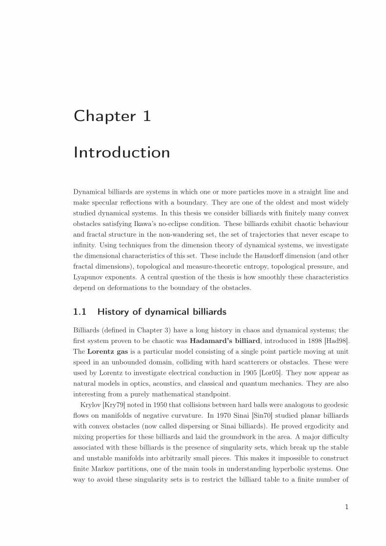
Dynamical billiards are systems in which one or more particles move in a straight line andmake specular reflections with a boundary. They are one of the oldest and most widelystudied dynamical systems. In this thesis we consider billiards with finitely many convexobstacles satisfying Ikawa’s no-eclipse condition. These billiards exhibit chaotic behaviourand fractal structure in the non-wandering set, the set of trajectories that never escape toinfinity. Using techniques from the dimension theory of dynamical systems, we investigatethe dimensional characteristics of this set. These include the Hausdorff dimension (and otherfractal dimensions), topological and measure-theoretic entropy, topological pressure, andLyapunov exponents. A central question of the thesis is how smoothly these characteristicsdepend on deformations to the boundary of the obstacles.

1.1 History of dynamical billiards

Billiards (defined in Chapter 3) have a long history in chaos and dynamical systems; thefirst system proven to be chaotic was Hadamard’s billiard, introduced in 1898 [Had98].The Lorentz gas is a particular model consisting of a single point particle moving at unitspeed in an unbounded domain, colliding with hard scatterers or obstacles. These wereused by Lorentz to investigate electrical conduction in 1905 [Lor05]. They now appear asnatural models in optics, acoustics, and classical and quantum mechanics. They are alsointeresting from a purely mathematical standpoint.

Krylov [Kry79] noted in 1950 that collisions between hard balls were analogous to geodesicflows on manifolds of negative curvature. In 1970 Sinai [Sin70] studied planar billiardswith convex obstacles (now called dispersing or Sinai billiards). He proved ergodicity andmixing properties for these billiards and laid the groundwork in the area. A major difficultyassociated with these billiards is the presence of singularity sets, which break up the stableand unstable manifolds into arbitrarily small pieces. This makes it impossible to constructfinite Markov partitions, one of the main tools in understanding hyperbolic systems. Oneway to avoid these singularity sets is to restrict the billiard table to a finite number of

1

1. Introduction

(a) A planar billiard with three disks. (b) A billiard in R3 with four spheres.

Figure 1.1: Non-wandering sets produced in Mathematica (Appendix B, Notebook 1).

obstacles satisfying a no-eclipse condition. These systems (which we will call non-eclipsingbilliards) were first described by Ikawa in 1988, in the context of studying the wave equation[Ika88]. They were later investigated in [Mor91, LM96, Sjö90, Sto89, Sto99, PS92], andmany others. Chernov refers to billiards that satisfy this condition as an “Ikawa-Moritagas” [Che91]. Gaspard and Rice considered a special case involving three disks [GR89] andfound a method to calculate the Hausdorff dimension of the non-wandering set.

The non-wandering set of an open billiard satisfying the no-eclipse condition is a visuallyinteresting fractal. Figure 1.1 shows the non-wandering set of the billiard outside threecircles arranged in an equilateral triangle, and Figure 1.1 shows the non-wandering set forfour spheres arranged in a regular tetrahedron. The cover image of this thesis shows arepresentation of the non-wandering set of a similar tetrahedron billiard, showing only thepositions of the non-wandering points on one of the spheres. These images were producedin Mathematica (see Appendix B, Notebook 1 in the CD included with this thesis). In anarticle published in Nature [SOY99], researchers built a model of a similar system withcoloured poster boards and cloth, and numerically estimated the Hausdorff dimension ofthe resulting fractal. Figure 1.2 shows two more physical models made with Christmasornaments.

1.2 Dimension theory of dynamical systems

The dimension theory of dynamical systems studies the dimensional characteristics of theinvariant sets of an iterated map or a flow. Fractal dimensions provide a way to intuitivelytalk about the "size" of a set, particularly sets that the usual topological dimension failsto describe. Invariant sets include strange attractors such as the Lorenz attractor [Lor63],repellers such as Julia sets, and hyperbolic sets, which include the non-wandering setfor a non-eclipsing billiard. The Hausdorff dimension is related to other dimensional

2

1.3. Outline and main results

(a) A close-up photo. (b) Four adjacent mirror balls from [Osk06].

Figure 1.2: Non-wandering sets produced in Mathematica (Appendix B, Notebook 1).

characteristics via Bowen’s equation, as we will see in Section 4.7.The first book on the theory was by Pesin [Pes97]. See [BG11] for a recent review of the

field. Past work has examined how dimensional characteristics of various dynamical systemscan change with respect to perturbations of the system. For example [KKPW89] showsthat the entropy of Anosov flows is differentiable, [Rue97] shows the same for SRB measuresin hyperbolic flows, and [Mañ90] differentiates the Hausdorff dimension of horseshoe sets.However this kind of problem has not been considered in the context of open billiardsystems satisfying the no-eclipse condition. One of the central results of this thesis is thatthe Hausdorff dimension of the non-wandering set for an open billiard in the plane dependssmoothly on perturbations to the boundary of the billiard.

1.3 Outline and main results

Although the focus is on the dimension theory of dynamical billiards, this thesis covers awide range of topics, including real analysis, differential geometry, matrix theory, ergodictheory, hyperbolic dynamics and geometry.

1.3.1 Chapter 2 — Preliminaries

In Chapter 2, we introduce some preliminary material and notations that will be used inthe thesis. This includes concepts from real analysis, differential geometry, matrix theorywith a focus on block matrices, and some miscellaneous notation.

1.3.2 Chapter 3 — Open billiards

In Chapter 3, we define dynamical billiards and the particular class of billiard investigatedin this thesis. We introduce Ikawa’s no-eclipse condition, the non-wandering set, somecrucial propositions concerning the periodic points in billiards, and some constants. Finallywe take an informal look at ways in which the conditions placed on a billiard can be relaxed.

3

1. Introduction

1.3.3 Chapter 4 — Dimension theory in dynamical systems

In Chapter 4, we define important concepts in dimension theory and dynamical systems,with a focus on hyperbolic dynamics. First we define various fractal dimensions, followed byrepellers and hyperbolic sets, and explain the coding of a dynamical system using a symbolspace and a Markov partition. We introduce Oseledets theorem, local product structure,and definitions of entropy and pressure. Finally we introduce some important theorems byPesin and Barreira, which use Bowen’s equation to calculate the Hausdorff dimension of aconformal hyperbolic invariant set. This will be used in Chapter 6.

1.3.4 Chapter 5 — Estimates of Hausdorff dimension of the non-wanderingset

In Chapter 5, we combine the information in the previous two chapters to obtain originalresults estimating the Hausdorff dimension of the non-wandering set of an open billiardin any dimension. This dimension D = dimH M0 was previously estimated in [Ken04] forbilliards in the plane, but Chapter 5 improves on these estimates and generalizes them tobilliards in any dimension. The central theorem of Chapter 5 is as follows.

Theorem 1.3.1. Consider a non-eclipsing open billiard in the exterior of a set K =

K1∪ . . .∪Km ⊂ RD, as defined in Chapter 3. Let B be the billiard ball map in Q = R

D\K.

We use the billiard constants defined in Section 3.6. Let g(γ, d) = γ2 +

√γ2

4 + γd and let

kmin, kmax be the minimum and maximum values of g over the following set:

D =⋃i,j,k

[2κ−k cosι φ+

ij,k,2κ+k

cosφ+ij,k

]× [d−jk, d

+jk],

where ι = 0 if D = 2 and ι = 1 if D > 2. Let

λ1 =1

1 + d+kmaxand μ1 =

1

1 + d−kmin,

Then the Hausdorff dimension of the non-wandering set M0 of B satisfies one of thefollowing:

(i) If D = 2, then−2 log(m− 1)

log λ1≤ dimH M0 ≤

−2 log(m− 1)

logμ1. (1.1)

(ii) If D > 2, and the obstacles Ki are sufficiently far apart that λd+1 < μ2d−

1 , then equation(1.1) holds.

(iii) Otherwise we have

ρ−2 log(m− 1)

log λ1≤ dimH M0 ≤ ρ−1−2 log(m− 1)

logμ1, (1.2)

where ρ ≤ 2d− log μ1

d+ log λ1is the Hölder constant of the local product map, as explained in

Section 5.9.

4

1.3. Outline and main results

The work in this chapter is original and has been published [Wri13]. It is an extension of[Ken04] to higher dimensions, with improved estimates.

1.3.5 Chapter 6 — Differentiability of Hausdorff dimension for planar bil-liards

In Chapter 6, we define deformations to billiards in the plane. We show that the points ofthe non-wandering set are differentiable with respect to these deformations under certainassumptions, and we estimate the derivatives. Then we use Bowen’s equation and Pesin’stheorem to estimate the derivative of dimH M0 with respect to a deformation. We obtainthe following theorems:

Theorem 1.3.2. Let K(α) be a planar billiard deformation satisfying the conditions inDefinition 6.2.1. Suppose the boundary of each obstacle is Cr, and depends Cr′-smoothly onα, with r ≥ 2, r′ ≥ 1. Then the non-wandering set M0 is Cmin{r−1,r′}-smooth with respectto α. Furthermore, the derivatives of the parameters that describe each point in M0 arebounded by constants that depend only on geometric properties of the deformation.

Using this theorem, we show that the curvature of convex fronts in the billiard dependsdifferentiably on α, and hence obtain the next theorem.

Theorem 1.3.3. Let K(α) be a planar billiard deformation as described above, but withr ≥ 4, r′ ≥ 3. For any α ∈ I, denote the Hausdorff dimension of the non-wandering set ofK(α) by

D(α) = dimH M0.

Then for any α ∈ I, the function D(α) is at least Cmin{r−3,r′−1} smooth. Furthermore, thereexists a constant Cψ = Cψ(α) depending only on geometric properties of the deformation,such that ∣∣∣∣dD(α)

dα

∣∣∣∣ ≤ CψD(α)

log(1 + d−kmin).

Finally, we show that if the billiard deformation K(α) is real analytic, then the Hausdorffdimension is a real analytic function of α. The work in this chapter is original and hasbeen submitted for publication [Wri14a].

1.3.6 Chapter 7 — Differentiability of Hausdorff dimension for nonplanarbilliards

In Chapter 7, we make an attempt to replicate the results of Chapter 6 for higher dimensionalbilliards. The points in the non-wandering set are still differentiable and are estimated bysimilar constants. However since the billiard map is not conformal in higher dimensions,the Hausdorff dimension is not known exactly. The main result is the following theorem.

5

1. Introduction

Theorem 1.3.4. Let K(α) be a billiard deformation in RD for D ≥ 3, satisfying the

conditions in Definition 7.2.1. Suppose the boundary of each obstacle is Cr, and depends Cr′-smoothly on α, with r ≥ 2, r′ ≥ 1. Then the non-wandering set M0 is Cmin{r−1,r′}-smoothwith respect to α. Furthermore, the derivatives of the parameters that describe each point inM0 are bounded by constants that depend only on geometric properties of the deformation.

We also obtain results for the derivative (with respect to α) of curvature of convex frontsin the billiard. The work in this chapter is original but has not yet been submitted forpublication.

1.3.7 Chapter 8 — Average conformal hyperbolic sets

In Chapter 8, we define the concept of an average conformal hyperbolic set, based on theconcept of an average conformal repeller introduced in [BCH10]. A hyperbolic set is averageconformal if there are exactly two Lyapunov exponents, one positive and one negative. Wefind an exact equation for the Hausdorff dimension of these sets. This chapter is not directlyrelated to billiards, but it may lead to further results that could solve a problem posed inChapter 7. It is possible that there exist a class of billiards such that the non-wanderingset is average conformal. The main result of Chapter 8 is the following theorem

Theorem 1.3.5. Let f : M → M be a hyperbolic diffeomorphism on a Riemannianmanifold, with a locally maximal hyperbolic set Λ, and let x ∈ Λ. Suppose Λ is averageconformal. Then for any x ∈ Λ,

dimH(Λ ∩W (u)(x)) = dimB(Λ ∩W (u)(x)) = dimB(Λ ∩W (u)(x))

=hκ(u)(f) dimE(u)(x)∫

Λ log | det (dxf |E(u)) |dκ(u),

dimH(Λ ∩W (s)(x)) = dimB(Λ ∩W (s)(x)) = dimB(Λ ∩W (s)(x))

=hκ(s)(f) dimE(s)(x)∫

Λ log | det (dxf |E(s)) |dκ(s).

where hκ(s)(f) and hκ(s)(f) are the entropies of f with respect to the unique equilibriummeasures κ(s) and κ(u) corresponding to log | det (dxf |E(s)) | and log | det (dxf |E(u)) | respec-tively.

The work in this chapter is original and has been submitted for publication [Wri14a]. Itis heavily inspired by [BCH10].

1.3.8 Chapter 9 — Examples and further research

In Chapter 9, we make some final remarks that don’t fit in the other chapters. We describethe Mathematica notebooks in Appendix B. Then we apply our results to a number ofexamples, and propose some further questions and open problems.

6

Chapter 2

Preliminaries

This chapter explains some preliminary information, definitions, notations and theoremsthat will be used in later chapters. Many of these are standard and well-known, but weinclude them for completeness. Some are extensions of a well known definition or fact, anda few are new.

2.1 Notation

Let A ⊂ RD with the standard Euclidean metric d.

• For x ∈ A, r > 0, denote by Br(x) the closed ball of radius r centred on x, and bySD−1 the unit sphere at the origin.

• Let ∂A be the boundary of A.

• Let Int(A) be the interior of A, i.e. the set of points of A that are not in the boundaryof A.

• Let diam(A) = maxx,y∈A

d(x, y) be the diameter of A.

• Let A be the closure of A.

• A is called convex if for every pair of points x, y ∈ A, the line segment between x

and y is entirely contained in A.

• Let Cvx(A) be the convex hull of A, i.e. the smallest convex set containing A.

Let M be a differentiable manifold, let B : M → M and f : M → R be differentiable maps,and let x ∈ M .

• Let TxM denote the tangent space of M at x.

• Let dxB denote the Jacobian matrix of B at x.

• For any vector w ∈ TxM , let ∇wf denote the directional derivative of ψ in thedirection w.

7

2. Preliminaries

2.2 Real analysis

2.2.1 Hölder and Lipschitz functions

Definition 2.2.1. For a number 0 < μ ≤ 1, a function between metric spacesf : X → Y is said to satisfy a Hölder condition or to be μ-Hölder continuous, if thereexists a constant C ≥ 0 such that for all x, y ∈ X,

‖f(x)− f(y)‖ ≤ C‖x− y‖μ.

The function f is said to be Lipschitz continuous if it is 1-Hölder continuous. Let �μ�denote the largest integer less than or equal to μ. For μ ∈ R

+\N, we say f is in Cμ if all thederivatives of f up to order �μ� are continuous, and f (�μ�) is (μ− �μ�)-Hölder continuous.

2.2.2 Differentiability classes for multiple variables

When f(x1, . . . , xn) is a function of n variables, sometimes we want to refer to the set ofall possible partial derivatives of order q.

Definition 2.2.2. Let X,Y be subsets of Euclidean spaces and let f : Xn → Y be afunction. It is common to define the vector operator

∇ =

(∂

∂x1, . . . ,

∂

∂xn

),

for x = (x1, . . . , xn). For higher derivatives, we will define the following set:

∇qf =

⎧⎨⎩ ∂qf∏n

j=1 ∂xqjj

: qj ∈ {0, . . . , q},n∑

j=1

qj = q

⎫⎬⎭ .

This set has nq elements. We use this notation in the following definitions. Let X,Y,A

be subsets of Euclidean spaces and let f : Xn → Y be a function. The convention fordifferentiability classes is to say that f is Cr in some open set U ⊂ R

n if every partialderivative of the form

∂pf

∂xp11 . . . ∂xpnn, p1 + . . .+ pn = p ≤ r

exists and is continuous in U . Or in the ∇q notation, we say each element of ∇pf iscontinuous for all p ≤ r. This convention is useful when the xi are all similar kinds ofvariables. However in this thesis we consider functions that depend on one deformationparameter and several billiard variables. So we use the following non-conventional notation.

Definition 2.2.3. Let X,Y,A be subsets of Euclidean spaces, let f : Xn × A → Y be afunction and let r, r′ be positive integers. Then we will say that f(x1, . . . , xn, α) is Cr,r′ atx = (x1, . . . , xn) ∈ Xn, α ∈ A, if for every p ≤ r, p′ ≤ r′, every element of the set

∂p′

∂αp′ ∇pf

exists and is continuous at (x, α) with respect to x and α.

8

2.2. Real analysis

Note that if f is Cr,r′ in the new notation, then it is Cmin{r,r′} in the conventional notation.Furthermore, if f is Cr in the conventional notation, then in the new notation it is Cr,r.

2.2.3 Cf notation

Frequently in Chapters 6 and 7 we will have some quantity that depends on a scalar α

and/or a vector (or sometimes a scalar) u, and we will show that its derivatives are boundedby some constants. Rather than numbering these constants, we will label them with thequantity being differentiated in the subscript and the number of differentiations in the

superscript. So for example if f is a function of α, we will say∣∣∣∣d2fdα2

∣∣∣∣ ≤ C(2)f . If g is a

function of u = (u0, . . . , un−1) and α, then we will say

∣∣∣∣∣ ∂q′

∂αq′ ∇qg

∣∣∣∣∣ ≤ C(q,q′)g , for any q, q′ ≥ 0

(as long as they are not both 0). These constants may depend on α, but not on u. Whenthere is only one variable and only the first derivative is required, we will simply write∣∣∣∣ dfdα

∣∣∣∣ ≤ Cf . We will explain what each constant refers to each time we use this notation.

2.2.4 Implicit function theorem

The implicit function theorem is very well known, and is central to the arguments inChapters 6 and 7. It gives sufficient conditions for an equation of the form f(x, y) = 0 tohave a solution y in terms of x.

Theorem 2.2.4. [AM78] Let f : Rn × Rm → R

m, (x, y) → f(x, y), be a Cr function.Suppose the Jacobian matrix J =

(∂fi∂yj

)mi,j=1

is invertible at a point (a, b) ∈ Rn×R

m. Then

there exists an open set U containing a, an open set V containing b, and a unique Cr

function y : U → V such that for all x ∈ U ,

f(x, y(x)) = 0.

For any i = 1, . . . ,m and j = 1, . . . , n, the derivatives ∂yj∂xi

can be found by solving thefollowing matrix equation.

∂fk∂xi

+

m∑j=1

Jjk∂yj∂xi

= 0 for all k = 1, . . .m.

Corollary 2.2.5. [KK83] If f is real analytic and also satisfies the conditions above, thenthe function y(x) is real analytic.

Corollary 2.2.6. If f is Cr,r′ and also satisfies the conditions above, then the functiony(x) is Cmin{r,r′} in standard notation.

Proof. Since f is Cr,r′ it is Cmin{r,r′}. So by the above theorem, y(x) is also Cmin{r,r′}.

9

2. Preliminaries

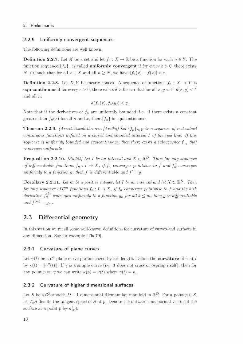
2.2.5 Uniformly convergent sequences

The following definitions are well known.

Definition 2.2.7. Let X be a set and let fn : X → R be a function for each n ∈ N. Thefunction sequence {fn}n is called uniformly convergent if for every ε > 0, there existsN > 0 such that for all x ∈ X and all n ≥ N , we have |fn(x)− f(x)| < ε.

Definition 2.2.8. Let X,Y be metric spaces. A sequence of functions fn : X → Y isequicontinuous if for every ε > 0, there exists δ > 0 such that for all x, y with d(x, y) < δ

and all n,d(fn(x), fn(y)) < ε.

Note that if the derivatives of fn are uniformly bounded, i.e. if there exists a constantgreater than fn(x) for all n and x, then {fn} is equicontinuous.

Theorem 2.2.9. (Arzelà Ascoli theorem [Arz95]) Let {fn}n∈N be a sequence of real-valuedcontinuous functions defined on a closed and bounded interval I of the real line. If thissequence is uniformly bounded and equicontinuous, then there exists a subsequence fnk

thatconverges uniformly.

Proposition 2.2.10. [Rud64] Let I be an interval and X ⊂ RD. Then for any sequence

of differentiable functions fn : I → X, if fn converges pointwise to f and f ′n converges

uniformly to a function g, then f is differentiable and f ′ = g.

Corollary 2.2.11. Let m be a positive integer, let I be an interval and let X ⊂ RD. Then

for any sequence of Cm functions fn : I → X, if fn converges pointwise to f and the k’thderivative f

(k)n converges uniformly to a function gk for all k ≤ m, then g is differentiable

and f (m) = gm.

2.3 Differential geometry

In this section we recall some well-known definitions for curvature of curves and surfaces inany dimension. See for example [Tho79].

2.3.1 Curvature of plane curves

Let γ(t) be a C2 plane curve parametrized by arc length. Define the curvature of γ at t

by κ(t) = ‖γ′′(t)‖. If γ is a simple curve (i.e. it does not cross or overlap itself), then forany point p on γ we can write κ(p) = κ(t) where γ(t) = p.

2.3.2 Curvature of higher dimensional surfaces

Let S be a C2-smooth D − 1 dimensional Riemannian manifold in RD. For a point p ∈ S,

let TpS denote the tangent space of S at p. Denote the outward unit normal vector of thesurface at a point p by n(p).

10

2.3. Differential geometry

Definition 2.3.1. Denote the directional derivative of a vector field F in the direction v

by ∇vF . Then the Weingarten map or shape operator Lp : TpS → TpS is defined by

Lp(v) = −∇vn.

The principle curvatures κ(1)(p), . . . , κ(D−1)(p) of S at p are the eigenvalues of the shapeoperator.

Definition 2.3.2. The first fundamental form of S at p is the inner product on thetangent space, or equivalently the quadratic form associated with the identity map on TpS.For any vectors u, v ∈ TpS,

Ip(v) = u · v.

Definition 2.3.3. The second fundamental form is the quadratic form associated withthe shape operator. It is given by

IIp(v, w) = 〈Lp(v), w〉.

It can also be represented as a matrix, as we will see.

2.3.3 Orthonormal parametrization

A set of vectors {v1, . . . , vn} is orthonormal if they are all unit vectors and all perpendicularto each other. Let S be a C2-smooth D − 1 dimensional surface in R

D and let p ∈ S. LetR ⊂ R

D−1 be a direct product of intervals and let S be parametrized by

ϕ : R → RD, u → ϕ(u),

such that the derivatives

du(1) =∂ϕ

∂u(1), . . . , du(D−1) =

∂ϕ

∂u(D−1)

are orthonormal vectors when ϕ(u) = p. We call this an orthonormal parametrizationof S at p. It is always possible to find such a parametrization. For any p ∈ S, denoteby U the rectangular matrix with the columns du(1), . . . , du(D−1) at p, and denote by W

the square matrix with the first D − 1 columns equal to U and with the unit normalvector nS(p) in the final column. Then W is orthonormal at p if the parametrization isorthonormal at p.

Using this parametrization, the matrix representing the first fundamental form of S at p

is UᵀU = ID−1, the identity matrix. The elements of the matrix representing the secondfundamental form are given by

IIst(p) =

⟨n(p),

∂2ϕ

∂us∂ut

⟩.

Thanks to the choice of parametrization, the principle curvatures κ(i) at p are the eigenvaluesof the matrix IIst(p).

11

2. Preliminaries

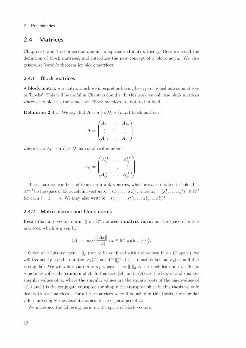
2.4 Matrices

Chapters 6 and 7 use a certain amount of specialised matrix theory. Here we recall thedefinition of block matrices, and introduce the new concept of a block norm. We alsogeneralise Varah’s theorem for block matrices.

2.4.1 Block matrices

A block matrix is a matrix which we interpret as having been partitioned into submatricesor ’blocks’. This will be useful in Chapters 6 and 7. In this work we only use block matriceswhere each block is the same size. Block matrices are notated in bold.

Definition 2.4.1. We say that A is a (n,D)× (n,D) block matrix if

A =

⎛⎜⎜⎝A11 . . . A1n

.... . .

...An1 . . . Ann

⎞⎟⎟⎠ ,

where each Aij is a D ×D matrix of real numbers.

Aij =

⎛⎜⎜⎝

A11ij . . . A1D

ij...

. . ....

AD1ij . . . ADD

ij

⎞⎟⎟⎠ .

Block matrices can be said to act on block vectors, which are also notated in bold. LetRn,D be the space of block column vectors x = (x1; . . . ;xn)

ᵀ, where xi = (x1i , . . . , xDi )ᵀ ∈ R

D

for each i = 1, . . . n. We may also write x = (x11, . . . , xD1 ; . . . ;x

1n, . . . x

Dn )

ᵀ.

2.4.2 Matrix norms and block norms

Recall that any vector norm ‖ on Rn induces a matrix norm on the space of n × n

matrices, which is given by

‖A‖ = max{‖Ax‖‖x‖ : x ∈ Rn with x �= 0}.

Given an arbitrary norm ‖ ‖p (not to be confused with the p-norm in an Lp space), wewill frequently use the notation σp(A) = ‖A−1‖−1

p if A is nonsingular and σp(A) = 0 if Ais singular. We will abbreviate σ = σ2 where ‖ ‖ = ‖ ‖2 is the Euclidean norm. This issometimes called the conorm of A. In this case ‖A‖ and σ(A) are the largest and smallestsingular values of A, where the singular values are the square roots of the eigenvalues ofA†A and † is the conjugate transpose (or simply the transpose since in this thesis we onlydeal with real matrices). For all the matrices we will be using in this thesis, the singularvalues are simply the absolute values of the eigenvalues of A.

We introduce the following norm on the space of block vectors.

12

2.4. Matrices

Definition 2.4.2. Let x ∈ Rn,D. Let ‖ ‖a be a norm on R

n and let ‖ ‖b be a norm on RD.

Then the block norm ‖ ‖a,b on Rn,D is defined by

‖x‖a,b =∥∥∥(‖x1‖a, . . . , ‖xn‖a)∥∥∥

b.

Let ‖ ‖∞ be the max norm on Rn, ‖x‖∞ = maxj |xj |. In Chapter 7 we will use the block

norm ‖ ‖2,∞.

Definition 2.4.3. Two norms ‖ ‖ and ‖ ‖′ are said to be equivalent if there exists aconstant C > 1 such that

1

C‖x‖′ ≤ ‖x‖ ≤ C‖x‖′.

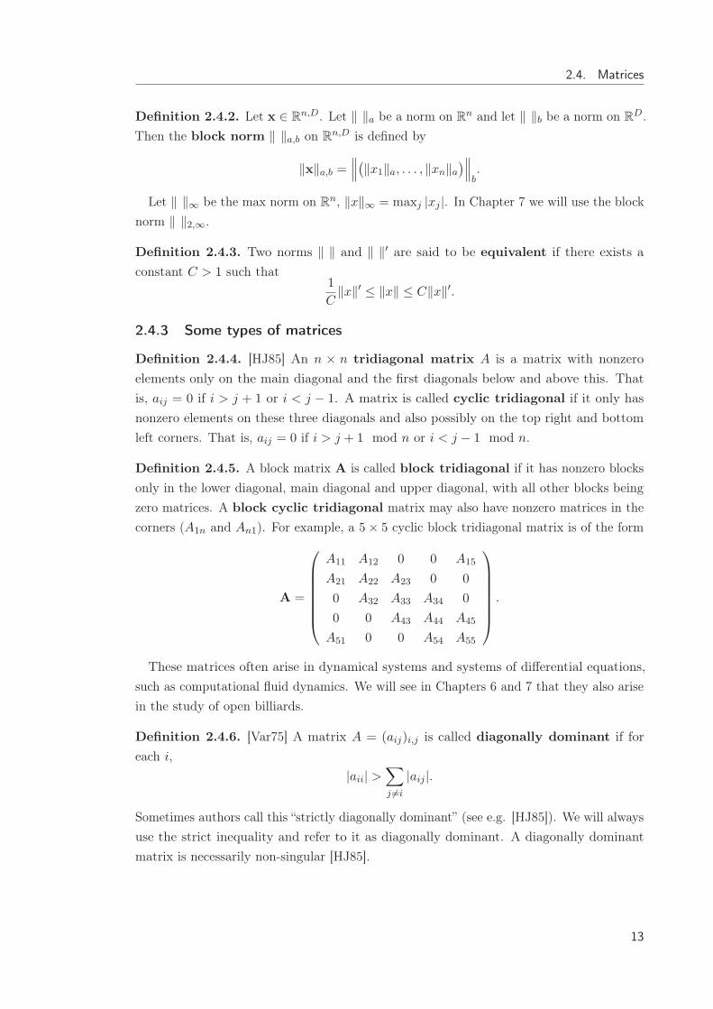
2.4.3 Some types of matrices

Definition 2.4.4. [HJ85] An n × n tridiagonal matrix A is a matrix with nonzeroelements only on the main diagonal and the first diagonals below and above this. Thatis, aij = 0 if i > j + 1 or i < j − 1. A matrix is called cyclic tridiagonal if it only hasnonzero elements on these three diagonals and also possibly on the top right and bottomleft corners. That is, aij = 0 if i > j + 1 mod n or i < j − 1 mod n.

Definition 2.4.5. A block matrix A is called block tridiagonal if it has nonzero blocksonly in the lower diagonal, main diagonal and upper diagonal, with all other blocks beingzero matrices. A block cyclic tridiagonal matrix may also have nonzero matrices in thecorners (A1n and An1). For example, a 5× 5 cyclic block tridiagonal matrix is of the form

A =

⎛⎜⎜⎜⎜⎜⎜⎝

A11 A12 0 0 A15

A21 A22 A23 0 0

0 A32 A33 A34 0

0 0 A43 A44 A45

A51 0 0 A54 A55

⎞⎟⎟⎟⎟⎟⎟⎠

.

These matrices often arise in dynamical systems and systems of differential equations,such as computational fluid dynamics. We will see in Chapters 6 and 7 that they also arisein the study of open billiards.

Definition 2.4.6. [Var75] A matrix A = (aij)i,j is called diagonally dominant if foreach i,

|aii| >∑j �=i

|aij |.

Sometimes authors call this “strictly diagonally dominant” (see e.g. [HJ85]). We will alwaysuse the strict inequality and refer to it as diagonally dominant. A diagonally dominantmatrix is necessarily non-singular [HJ85].

13

2. Preliminaries

Definition 2.4.7. A block matrix A will be called weakly block diagonally dominant(WBDD) with respect to a matrix norm ‖ ‖p (on the space of D×D matrices) if for each i,

σp(Aii) >∑j �=i

σp(Aij).

Definition 2.4.8. A block matrix A will be called strongly block diagonally dominant(SBDD) with respect to a norm ‖ ‖p if for each i,

σp(Aii) >∑j �=i

‖Aij‖p.

For p = ∞, this last condition is simply called “block diagonally dominant” in [Var75]. It iseasy to see that if a matrix is strongly block diagonally dominant then it is nonsingularand weakly block diagonally dominant.

2.4.4 Varah’s theorem and extensions

The following theorem is due to Varah. We will use it in Chapter 6.

Theorem 2.4.9. [Var75] Let A = (aij)nij be a diagonally dominant matrix. Then we have

‖A−1‖∞ ≤ 1h , where

h = mini

⎛⎝|aii| −

∑j �=i

|aij |

⎞⎠ .

Varah extended this theorem to SBDD matrices with respect to the norm ‖ ‖∞.

Theorem 2.4.10. (Varah’s theorem for SBDD matrices). Let A = (Aij)nij, Aij ∈ R

D×D

be a strongly block diagonally dominant matrix with respect to ‖ ‖∞. Then ‖A−1‖∞ ≤ 1h ,

where

h = mini

⎛⎝σ∞(Aii)−

∑j �=i

‖Aij‖∞

⎞⎠ .

However in Chapter 7 we use a different version of the theorem that applies to WBDDmatrices and uses block norms.

Theorem 2.4.11. (Varah’s theorem for WBDD matrices). Let ‖ ‖p be a norm on RD, and

let A = (Aij)nij, Aij ∈ R

D×D be a nonsingular weakly block diagonally dominant matrix.Then ‖A−1‖∞,p ≤ 1

h , where

h = mini

⎛⎝σp(Aii)−

∑j �=i

σp(Aij)

⎞⎠ .

Proof. The proof is similar to the proof of Varah’s theorem in [Var75]. Since

‖A−1‖−1∞,p = inf

x

‖A x‖∞,p

‖x‖∞,p,

14

2.4. Matrices

we only need to show that h‖x‖∞,p ≤ ‖A x‖∞,b for all x. Choose an arbitrary x ∈ Rn,D

and choose i such that ‖xi‖p = ‖x‖∞,p. Then since A is WBDD,

0 ≤ h ≤ σp(Aii)−∑j �=i

σp(Aij),

h‖xi‖p ≤ σp(Aii)‖xi‖p −∑j �=i

σp(Aij)‖xi‖p

≤n∑

j=1

σp(Aij)‖xi‖p ≤ maxi

n∑j=1

‖Aijxi‖p

≤ ‖A x‖∞,p.

15

Chapter 3

Open billiards

3.1 Billiards

Generally, a billiard is a dynamical system in which one or more particles move in somedomain Q ⊂ R

D and collide with the boundary ∂Q or with each other. In this work wespecifically consider billiards in which a single pointlike particle moves in straight lines atconstant speed in Q and reflects off the boundary ∂Q according to the classical laws ofoptics. Dynamical billiards appear as natural models in optics, acoustics, and classical andquantum mechanics. A billiard with multiple particles can often be reduced to a billiardwith a single particle in a higher dimensional space (see e.g. [CM06, Section 1.3]). Similarlya system with a moving ball of some radius r can be shown to be equivalent to a systeminvolving a point particle.

Collisions with the boundary are specular reflections, that is, the angle of incidenceequals the angle of reflection. We describe a particle in the billiard by xt = (qt, vt) whereqt ∈ Q is the position of the particle and vt ∈ S

D−1 is its velocity at time t. Then for aslong as the particle stays inside Q, it satisfies

(qt+s, vt+s) = Ss(xt) = (qt + svt, vt).

Collisions with the boundary are described by

v+ = v− − 2〈v−, n〉n,

where n is the normal vector (into Q) of ∂Q at the point of collision, v− is the velocitybefore reflection and v+ is the velocity after reflection. We denote the angle between v−

and n (or between n and v+) by φ. The map St is a group action of R onto Q× SD−1 and

is known as the billiard flow. Figure 3.1 shows an example of a reflection.A connected component of the boundary ∂Q is called semi-dispersing if it is convex

(curving into Q), dispersing if it is strictly convex, and focusing if it is concave (curvingaway from Q). Sinai studied billiards that are everywhere dispersing in his influential paper[Sin70]. These billiards are now known as Sinai billiards. For an introduction to planarbilliards that exhibit chaotic behaviour, see Chernov and Markarian’s book [CM06].

17

3. Open billiards

Figure 3.1: A reflection in an open billiard, showing the normal vector and collision angleat x = (q, v) and Bx.

Open billiards are a class of billiards in which the domain Q is unbounded. In this thesiswe will consider open billiards in Q = QK = R

D\K, where

K = K1 ∪ . . . ∪Km

is a union of pairwise disjoint, compact and strictly convex sets with Cr boundary, forsome integers m ≥ 3 and r ≥ 2. The Ki are known as obstacles or scatterers. For anyx = (q, v) with q ∈ ∂K, we denote by n(q) = nK(q) the outward unit normal vector of∂K at q, and by φ(x) the collision angle between v and n. Since n(q) involves the firstderivative, it is Cr−1 and therefore Stx is a Cr−1 function of x.

One problem with billiard systems is that they often have singularities at the pointswhere a billiard trajectory is tangent to an obstacle. At these points the derivatives of thebilliard flow are unbounded, and images and preimages of singularities make a dense set inthe phase space. A way to avoid singularities is to assume that the following no-eclipsecondition holds, often known as condition (H).

Definition 3.1.1. A billiard in the exterior of K satisfies the condition (H) if for anynonequal i, j, k, the convex hull of Ki ∪ Kj does not intersect Kk. That is, no obstacle“eclipses” the path between two obstacles.

This condition was introduced by Ikawa [Ika88] in 1988. It ensures that the collisionangle φ is bounded above by a constant φ+ < π

2 , and thus prevents discontinuities inthe non-wandering set M0, as we will see later. These billiards have been investigated in[Mor91, LM96, Sjö90, Sto89, Sto99, PS92] and many others. Chernov refers to billiards

18

3.1. Billiards

that satisfy this condition as an “Ikawa-Morita gas” [Che91]. Let

Q = {(q, v) ∈ Q× SD−1 : q ∈ Int(Q) or 〈n, v〉 ≥ 0}.

This is the phase space of the flow St. It consists of particles that are either inside Q

(not on the boundary), or on the boundary and moving into Q. We define the canonicalprojection π : Q → Q by (q, v) → q. For any x = (q, v) ∈ Q, we denote by tj(q, v) ∈[−∞,∞] the time of the j-th reflection of x, with the convention that t0(q, v) = t1(q,−v)

if q ∈ Int(Q), or t0(q, v) = 0 if q ∈ ∂Q. We say tj(x) = ∞ if the forward trajectory of xdoes not have at least j reflections, and tj(x) = −∞ if the backward trajectory does nothave at least j reflections. Let dj(x) = tj(x)− tj−1(x) and abbreviate d(x) = d1(x). Letφj(x) be the collision angle at the j’th collision.

3.1.1 The billiard ball map

So far we have considered billiards as a flow. However the system can also be described bya map from one reflection to the next. Let

M = {(q, v) ∈ ∂K × SD−1 : 〈n(q), v〉 > 0}.

This is the set of particles confined to the boundary of Q. Then let

M ′ = {x ∈ M : t1(x) < ∞}.

Then define the billiard ball map as

B : M ′ → M,x → St1(x)(x).

This is a Cr−1 map. Define the reflection map Refl: Q → Q by

Refl(q, v) =

{(q,−v), for q ∈ Int(Q),

(q, 2〈nK(q), v〉nK(q)− v〉), for q ∈ ∂K.

This simply reverses the direction of a particle. Since the normal vector n(q) uses the firstderivative, it is Cr−1, so the reflection map is also Cr−1.

3.1.2 Non-wandering set

A point x is called non-wandering if tj(x) < ∞ for all j ∈ Z. The non-wanderingset of the flow is the set of non-wandering points in Q, and is denoted Ω(S) or Ω. Itsrestriction to the boundary of K is the non-wandering set of the billiard ball map B:M0 = Ω ∩ (∂K × S

D−1). Equivalently,

M0 = {x ∈ M : |tj(x)| < ∞, ∀j ∈ Z}.

Both non-wandering sets are invariant, meaning that if x ∈ M0 then Bx ∈ M0, and ifx ∈ Ω then St ∈ Ω for all t ∈ R. As we will see in Chapter 4, the billiard ball map is anexample of an axiom A diffeomorphism, and the billiard flow is an axiom A flow.

19

3. Open billiards

Definition 3.1.2. A billiard will be called degenerate if its non-wandering set is confinedto a hyperplane of smaller dimension than the billiard. For example, a billiard consistingof spheres with centres in the plane z = 0 is degenerate, because although the billiard isthree dimensional, its non-wandering set is confined to the plane.

Proposition 3.1.3. The billiard ball map is invertible and both the map and its inverseare Cr−1 when restricted to M0.

Proof. Let x ∈ (q, v) ∈ M0. Then let y = Refl(B(Reflx)). Then y ∈ M0, and a quickgeometrical argument shows that By = x, so y = B−1x. Since Refl is Cr−1, B and itsinverse are also Cr−1.

3.1.3 The phase space of the billiard as a Riemannian manifold

Points in the tangent space TxM are denoted (dq, dv). On the tangent space we can usethe inner product from the manifolds ∂K to define an inner product on M . At any pointx = (q, v) we have

〈(dq, dv), (dq′, dv′)〉 = 〈dq, dq′〉 cosφ,

where φ is the collision angle at x. This inner product induces a norm ‖(dq, dv)‖ = |dq| cosφon M . The set M together with this inner product is a Cr Riemannian manifold.

3.2 Parametrization

In this section we will assume that D ≥ 3 unless stated otherwise. Consider a billiard inQK with Cr smooth boundaries ∂Ki satisfying (H). For any point p ∈ ∂K, we can choosea parametrization of the obstacle boundary containing p that has orthonormal derivativesat p. So rather than using a single consistent parametrization for each obstacle, it will beeasier (in this thesis at least) to use a new parametrization for every collision.

Let x = (q, v) ∈ M0. This generates a list of points p = (. . . , p−1, p0, p1, . . .) withpj = πBjx ∈ Kξj , where ξi ∈ {1, . . . ,m}. Let Rj ⊂ R

D−1 be a direct product of intervalsand let

ϕj : Rj → RD, uj → ϕj(uj)

parametrize ∂Kξj such that the derivatives du(1)j , . . . , du

(D−1)j =

∂ϕj

∂u(1)j

, . . . ,∂ϕj

∂u(D−1)j

are

orthonormal when ϕj(uj) = pj . That is, all the vectors are unit vectors and perpendicularto each other. We call this an orthonormal parametrization of Kξj at pj . Note thateach obstacle can have many different parametrizations. For example if ξ1 = ξ3 = 2, then∂K2 will have at least two parametrizations, ϕ1 and ϕ3, and these may be different.

Definition 3.2.1. Denote by Uj the rectangular matrix with columns du(1)j , . . . , du

(D−1)j ,

and denote by Wj the square matrix equal to Uj except with the unit normal vector nK(pj)

20

3.2. Parametrization

in the final column. That is,

Wj =

⎛⎜⎜⎜⎜⎜⎝

∂ϕ(1)j

∂u(1)j

. . .∂ϕ

(1)j

∂u(D−1)j

n(1)(pj)

.... . .

......

∂ϕ(D)j

∂u(1)j

. . .∂ϕ

(D)j

∂u(D−1)j

n(d)(pj)

⎞⎟⎟⎟⎟⎟⎠

If ϕj is an orthonormal parametrization at pj then Wj is an orthogonal matrix at pj .

Example 3.2.2. We use the unit sphere at the origin as an example. The conventionalparametrization for S

2 is

ϕ(u, v) =

⎛⎜⎝sinu cos v

sinu sin v

cosu

⎞⎟⎠ .

For any point p ∈ S2 except for the poles, let up, vp be the parameters satisfying ϕ(up, vp) = p.

Then define

ϕp(u, v) = ϕ

(u+ up,

v + vpsinup

)=

⎛⎜⎜⎝sin(u+ up) cos

(v+vpsinup

)sin(u+ up) sin

(v+vpsinup

)cos(u+ up)

⎞⎟⎟⎠ .

In this parametrization, the domain is Rp = [0, τ ] × [0, τ sinup]. It is easy to check thatϕp(0, 0) = p and that the derivatives ∂ϕp

∂u ,∂ϕp

∂v are orthonormal at p. Note that at the polesof the sphere these parametrizations are undefined. However we can find orthonormalparametrizations at these points by using a different starting parametrization ϕ. For sphereswith centre a and radius r we can define

ϕp(u, v) = a+ rϕ

(u+ up

r,v + vpr sinup

).

For ellipsoids and other non-spherical obstacles, it may be difficult to find an explicitorthonormal parametrization, but it always exists by abstract arguments.

3.2.1 Curvature

Using an orthonormal parametrization at pj , the matrix representing the first fundamentalform of Kξj at pj is Uᵀ

j Uj = ID−1, the identity matrix. The elements of the (D−1)×(D−1)

matrix representing the second fundamental form are given by IIlmj =

⟨n(pj),

∂2ϕ∂ul

j∂umj

⟩.

The principle curvatures κ(i)j at pj are the eigenvalues of IIlmj at pj . Since the boundaries

are strictly convex, the principle curvatures are bounded by κmin(pj) ≤ κ(i)j (pj) ≤ κmax(pj),

and these are themselves bounded by positive constants κ− below and κ+ above.

21

3. Open billiards

3.2.2 Planar billiards

For billiards in the plane, the situation is much simpler. The boundary of each obstacleis a plane curve, and we can always choose to parametrize by arc length over the wholeobstacle. For each i = 1, . . . ,m, let ϕi(u) parametrize Ki counterclockwise by arc length.We denote the curvature of ∂K at q by κ(x), and at πBjx by κj(x). Since the boundariesare strictly convex, these are bounded by constants κ− ≤ κmin(x) ≤ κ ≤ κmax(x) ≤ κ+.

3.3 Periodic points

A point x = (q, v) ∈ M is called periodic with period n if Bnx = x. Let Mn ⊂ M0 be theset of n-periodic trajectories. It is common to describe a dynamical system using a spaceof sequences of symbols. We will see a general version of this in Chapter 4. Define then-periodic symbol space by

Σn = {ξ = (ξ0, . . . , ξn−1) : ξi ∈ {1, . . .m}, ξi �= ξi+1, ξn−1 �= ξ0}.

A finite sequence ξ of symbols {1, . . . ,m} satisfying ξn−1 �= ξ0 and ξi �= ξi+1 for all i is calleda finite admissible sequence. We often use the convention that ξn = ξ0. For example,a periodic trajectory that hits the obstacles K2,K3,K1,K3,K1 before repeating can bedescribed uniquely by the string “(2,3,1,3,1)”. The reason for the condition ξi �= ξi+1 is thatif all the obstacles are convex, a trajectory cannot leave ∂Ki, travel in a straight line, andhit the same ∂Ki. Define the representation map ξ : Mn → Σn by ξ(x) = (ξ0, . . . , ξn−1),where πBjx ∈ Kξj . We denote Kξ = Kξ0 × . . . × Kξn−1 . The periodic points can bedetermined by minimising the length function F that gives the length of a polygon withpoints restricted to particular obstacles, as shown in the following section.

3.3.1 Length function

Let the length function F = Fξ : Kξ → R be defined by

F (q0, . . . , qn−1) =

n−1∑j=0

‖qj − qj+1‖,

where we write qn = q0.

Lemma 3.3.1. (Periodic points lemma) Consider an open billiard in QK ,K = K1∪. . .∪Km

satisfying (H). Then for a fixed string ξ ∈ Σn the function Fξ has exactly one minimum at

p = (p0, . . . , pn−1).

These points determine a billiard trajectory that satisfies the classical laws of optics, that is,if vj =

pj+1−pj‖pj+1−pj‖ then (pj+1, vj+1) = B(pj , vj).

Proof. The first full proof of this lemma can be found in [Sto89], however versions of it canbe found in [Ika88] and [Sjö90].

22

3.4. Symbolic dynamics

This shows that the representation map ξ is invertible. Its inverse is χξ = (p0, v01),where v01 is the unit vector from p0 to p1, and the points pi are found by minimizing thelength function.

Now for each j, let Rj ⊂ RD−1 be a direct product of intervals, let Rξ = Rξ0× . . .×Rξn−1 ,

and let ϕj(uj) be a parametrization of ∂Kξj that is orthonormal at pj . Consider the functionGξ : Rξ → R defined by G(u0, . . . un−1) = F (ϕξ0(u0), . . . ϕξn−1(un−1)).

Corollary 3.3.2. Consider an open billiard in QK satisfying (H). Then for a fixed sequenceξ the function Gξ has exactly one minimum at

u = (u0, . . . , un−1), uj ∈ Rj .

The corresponding minimum of Fξ is given by

(p0, . . . , pn−1) = (ϕξ0(u0), . . . , ϕξn−1(un−1)).

Example 3.3.3. Consider a billiard with three obstacles, K = K1 ∪K2 ∪K3, and let ξ bethe period 3 sequence (1, 2, 3). There exists exactly one trajectory x satisfying

• B3x = x ∈ ∂K1,

• Bx ∈ ∂K2,

• B2x ∈ ∂K3.

To find it, find the shortest (by perimeter) triangle with vertices p1 ∈ ∂K1, p2 ∈ ∂K2, p3 ∈∂K3. Then x is the pair

(p1,

p2−p1‖p2−p1‖

).

3.4 Symbolic dynamics

Define the symbol space for the whole non-wandering set by

Σ = {ξ = (. . . , ξ−1, ξ0, ξ1, . . .) : ξi ∈ {1, . . .m}, ξi �= ξi+1}.

Define the representation map ξ : M0 → Σ by ξ(x) = (. . . , ξ−1, ξ0, ξ1, . . .), where πBjx ∈Kξj . Let the two-sided subshift σ : Σ → Σ be defined by (σξ)i = ξi+1. Then σ iscontinuous under the following metric dθ for any θ ∈ (0, 1).

dθ(ξ, ξ′) =

⎧⎨⎩0 : if ξi = ξ′i for all i ∈ Z

θn : if n = max{j ≥ 0 : ξi = ξ′i for all |i| < j},

Define the following equivalence relations on Σ. For any positive integer n and any sequencesξ, ξ′ ∈ Σ, we say ξ ∼n ξ′ if ξj = ξ′j for all |j| ≤ n. Similarly for x, y ∈ M0 we say x ∼n y ifξ(x) ∼n ξ(y). This means that two points are n-equivalent if Bjx and Bjy are on the sameobstacle Kξj for all |j| ≤ n. The equivalence class [ξ]n of sequences ξ′ such that ξ ∼n ξ′ iscalled an n-cylinder of ξ. Define another relation (not an equivalence relation) ≈m on Σ

by ξ ≈m ξ′ if ξ ∼m ξ′ and ξm+1 �= ξ′m+1.

23

3. Open billiards

Theorem 3.4.1. [Sjö90] There exist constants C > 0, δ ∈ (0, 1) such for that anyx, y ∈ B−nM,n ≥ 1 with points pj = πBjx, qj = πBjy lying in the same obstacleboundaries ∂Kξj , (with ξj ∈ {1, . . . ,m}, j = 0, . . . , n), we have

‖pj − qj‖ ≤ C(δj + δn−j)

for all j = 0, . . . , n.

Proof. See of [Sjö90, Appendix b], or [PS92, Lemma 10.2.1].

Corollary 3.4.2. For the same constants C > 0, δ ∈ (0, 1) as above, for any pointsx, y ∈ M0 with pj = πBjx, qj = πBjy lying on the same obstacle boundaries ∂Kξj forj = −n, . . . , 0, . . . , n, then

‖πx− πy‖ ≤ 2Cδn.

Proof. Let x′ = B−nx and y′ = B−ny, then apply Theorem 3.4.1 to Bnx′, Bny′.

Proposition 3.4.3. The periodic points are dense in M0, meaning that for every pointx ∈ M0, any neighbourhood of x contains at least one periodic point.

Proof. Since x → ξ is a homeomorphism, it is enough to prove that Σn is dense in Σ.Let ξ ∈ Σ and for each n > 1 define a sequence of periodic sequences {ξ(n)}n in Σ byξ(n)j = ξ(j mod n), so that ξ(n) ∈ Σn. As n → ∞ we have

dθ(ξ, ξ(n)) ≤ θn → 0,

so Σn is dense in Σ.

Corollary 3.4.4. Let ξ ∈ Σ, and define a sequence of periodic sequences {ξ(n)}n in Σ byξ(n)j = ξ(j mod n), so that ξ and ξ(n) are on the same n-cylinder. Note that ξ(n) is equivalent

to a string in Σn. Then the following limit exists:

χ(ξ) = limn→∞χ

(ξ(n)

),

and χ : Σ → M0 is the inverse of ξ : M0 → Σ.

Proof. We have‖χξ − χξ(n)‖ ≤ Cδn → 0,

so χξ(n) absolutely converges to χξ.

The following diagrams commute:

MnB �� Mn

Σn σ��

χ

��

Σn

χ

�� and M0B �� M0

Σ0 σ��

χ

��

Σ0

χ

�� .

Theorem 3.4.5. If θ ∈ (0, 1), then χ is a homeomorphism of M0 (with the topology inducedby M) onto (Σ, dθ), and the shift σ is topologically conjugate to B, that is B = χ−1 ◦ σ ◦ χ.

Proof. This is well-known, see e.g. [Mor91, Sto99], or [Ken04] for the exact statement insimilar notation.

24

3.5. Relaxing conditions

Figure 3.2: This open billiard is not convex or differentiable, and it violates the no-eclipsecondition, but it does not have singularities in the non-wandering set. For this billiard thenon-wandering set is the union of a Cantor-like subset of the shaded area with the isolatedorbit between K3 and K4.

3.5 Relaxing conditions

This section is an informal analysis of open billiards that do not satisfy the conditions wehave placed on them so far, such as convexity, smoothness and the no-eclipse condition.Some of these conditions can be relaxed, in the sense that violations can be ignored if theyare sufficiently “out of the way”. Figure 3.2 shows a billiard that clearly violates threedifferent conditions, but these violations can be safely ignored because they occur outsidethe interesting part of the billiard, namely the non-wandering set. The non-wanderingset M0 in that example consists of two parts: one is confined to the shaded area, whilethe other is a degenerate set consisting of only two points. A full investigation of whenviolations can be ignored would be difficult and not particularly useful, but we do have aconjecture that confines the non-wandering set to the following region:

Definition 3.5.1. For any i �= j, let (pij , pji) ∈ Ki × Kj denote the minimum of F :

Ki ×Kj → R, (q1, q2) → ‖q1 − q2‖. These are the pairs of period 2 points. Then each pij ison the boundary ∂Ki and the vector pji − pij is normal to ∂Ki at pij . Define the followingconvex hull of period 2 orbits:

H2 = Cvx ({pij : 1 ≤ i, j ≤ n, i �= j} ∩Q) .

25

3. Open billiards

A more sophisticated definition may be possible for billiards that are not convex, notdifferentiable, or that violate the no-eclipse condition.

Conjecture 3.5.2 (Convex hull conjecture). Let ξ0, . . . , ξn−1 (n ≥ 3) be a finite sequenceof indices and let (q0, . . . , qn−1) be a periodic billiard trajectory such that qj ∈ Kξj for eachj. Then each qj is contained in H2. Furthermore, the non-wandering set M0 is containedin H2.

We prove this conjecture for the case of a 3-dimensional billiard in which the obstaclesare spheres. A very similar proof will work for all two-dimensional billiards, and for higherdimensional billiards with hyperspherical obstacles. We leave the general case in higherdimensions as an open problem.

Proof for three dimensional billiards with spherical obstacles. If the obstacles are spheres,then H2 ∩ Q is simply the convex hull of the centres of the spheres intersected with Q.Suppose that (q0, . . . , qn−1) is a periodic trajectory, but that at least one point is outsideH2. Without loss of generality we can number the points and obstacles such that q1 /∈ H2

and ξ1 = 1. H2 is bounded by a number of planes, so q1 ∈ K1 is on the outside (i.e. theside not containing H2) of one such plane, say Π = Π123, determined by the centres ofobstacles K1,K2,K3. Let ν be the outward normal vector of Π and denote vj =

qj+1−qj‖qj+1−qj‖ ,

(with the convention that q0 = qn). Without loss of generality, assume that v0 · ν > 0. Foreach k ≥ 1 we have qk+1 = qk + dkvk and vk = vk−1 − 2〈vk−1, nK(qk)〉nK(qk). We alsohave 〈vk−1, nK(qk)〉 < 0. We show by induction that qk · ν > q1 · ν and vk−1 · ν > v0 · ν forall k > 1.

Suppose qk ∈ ∂Kαkis on the outside of Π and vk−1 · ν > v0 · ν. The centre of

∂Kαkis on the inside of Π, so the normal vector n(qk) must point away from Π, i.e.

nK(qk) · ν > 0. So vk · ν = vk−1 · ν − 2〈vk−1, nK(qk)〉nK(qk) · ν > vk−1 · ν > v0 · ν. Thenqk+1 · ν = qk · ν + dkvk · ν > qk · ν. So qk+1 is also on the outside.

For the orbit to be periodic we must have q0 = qn for some n. So by contradiction, allperiodic points must be contained in H2. Since H2 is a closed set and the periodic pointsare dense in M0, we have M0 ⊂ H2.

Corollary 3.5.3. Informally, anything that happens outside of H2 without changing thestructure of H2 can be essentially ignored, since it will not affect M0.

3.6 Billiard constants

In this section we define some constants that bound the distances, curvatures and collisionangles associated with each billiard. These constants will be called billiard constants.

26

3.6. Billiard constants

First we define the following sets:

Γi = {x ∈ M0 : πx ∈ ∂Ki}Γij = {x ∈ M0 : πx ∈ ∂Ki, πBx ∈ ∂Kj}

Γξ = Γξ0,...,ξn = {x ∈ M0 : πBjx ∈ ∂Kξj , j = 0, . . . , n}.

So Γij is the set of non-wandering trajectories in Ki that are heading for Kj . The notationfor billiard constants is as follows: a superscript ′−′ indicates a minimum, a superscript ′+′

indicates a maximum, and the subscripts indicate the relevant obstacles.

3.6.1 Distances

For any i, j = 1, . . . ,m with i �= j, denote

d−ij = min{d(x) : x ∈ Γij}d+ij = max{d(x) : x ∈ Γij}d− = min{d−ij : i, j ∈ {1, . . . ,m}}d+ = max{d+ij : i, j ∈ {1, . . . ,m}}.

So for example, d+23 is the maximum distance between obstacles K2 and K3 when confinedto the non-wandering set.

3.6.2 Curvatures

Recall that the second fundamental form II(p) of K has D − 1 eigenvalues, κ(j)(p), whichare the principle curvatures at p. For each i = 1, . . . ,m, denote

κ−i = min{κ(j)(q) : j ∈ {1, . . . , D − 1}, (q, v) ∈ Γi}κ+i = max{κ(j)(q) : j ∈ {1, . . . , D − 1}, (q, v) ∈ Γi}κ− = min

iκ−i

κ+ = maxi

κ+i .

3.6.3 Collision angles

Recall that the collision angle at x = (q, v) is the angle between v and n(q), i.e. cosφ(x) =

〈v, n〉. The collision angles are bounded below by 0, so we only define the maximum angles

φ+ij,k = max{φ(x) : B−1x ∈ Γikj},

φ+ = maxi,j,k

φ+ij,k.

Then φ+ij,k is the maximum angle for any trajectory coming from Ki, currently on Kk, and

going to Kj .

27

3. Open billiards

3.6.4 Estimating billiard constants

The above billiard constants can be estimated quite accurately and easily by using H2 inplace of M0. The following are the estimates used in Appendix A, Notebook 2.

Clearly the constants d−ij are given by the lengths of the period 2 orbits. The constantsd+ij satisfy

d+ij ≤ max{d(x) : x,Bx ∈ M,πx ∈ ∂Ki ∩H2, πBx ∈ ∂Kj ∩H2}.

The minimum and maximum curvatures over M0 can be estimated by

κ−i ≤ minq∈∂Ki∩H2

κmin(q) and κ+i ≤ minq∈∂Ki∩H2

κmax(q).

Letbij,k = min

kd(Kk ∩H2,Cvx (Ki ∩H2,Kj ∩H2)

).

Then we have

φ+ij,k ≤ arccos

⎛⎝ b−ij,kmax

{d+ik, d

+jk

}⎞⎠ .

The proof of this follows the proof in [Ken04, Section 3]. The reason for using this estimateis that bij,k is often easier to measure in practice than φ+

ij,k.

28

Chapter 4

Dimension theory in dynamicalsystems

4.1 Introduction

In this chapter we provide some background on the dimension theory of dynamical systems.This field studies the dimensional characteristics (such as Hausdorff dimension) of theinvariant sets and measures of dynamical systems. The first book on this theory was byPesin [Pes97]. See [BG11] for a recent review of this field. Throughout this chapter aresome remarks relating the concepts back to billiards.

4.2 Fractal dimensions

A fractal dimension is an extension of topological dimension that can take non-integervalues for some sets. Famous examples of fractals that have non-integer dimension includethe Cantor set, the Sierpinski triangle and the Koch curve. The non-wandering set of anopen billiard is a less well known example.

4.2.1 Hausdorff dimension

The Hausdorff dimension is the oldest and most important of the fractal dimensions [Fal90].Let X be a separable metric space. Given a set Z ⊂ X and a number s > 0, we define thes-dimensional Hausdorff measure of Z by

Hs(Z) = limε→0

infU

∑U∈U

diam(U)s,

where the infimum is over all countable covers U of Z by open sets U with diam(U) ≤ ε.The Hausdorff dimension of Z is defined by

dimH Z = inf{s > 0 : Hs(Z) = 0}.

29

4. Dimension theory in dynamical systems

Proposition 4.2.1. [Fal90] Let Z ⊂ Rn and let f : Z → R

m be a μ-Hölder continuousfunction. Then

dimH f(Z) ≤ 1

μdimH Z.

Corollary 4.2.2. If f is bi-Hölder continuous with Hölder constant μ, then

μ dimH Z ≤ dimH f(Z) ≤ 1

μdimH Z.

Furthermore, if f is bi-Lipschitz, then dimH f(Z) = dimH Z.

4.2.2 Box dimension

The box-counting or box dimensions are also widely used. Let N(Z, ε) be the number ofballs of radius ε needed to cover Z. Then the lower and upper box dimensions of Z arerespectively defined by

dimBZ = lim infε→0

logN(Z, ε)

− log εand dimBZ = lim sup

ε→0

logN(Z, ε)

− log ε.

4.2.3 Packing dimension

Let

Psε (Z) = sup

{∑B∈B

diam(B)s :B is a collection of disjoint ballsof radii at most ε with centres in Z

}.

Then define the s-dimensional packing measure of Z by

Ps = inf

{∑i

limε→0

Psε (Zi) : Z ⊂

∞⋃i=1

Zi

}

The packing dimension of Z is defined by

dimH Z = inf{s > 0 : Ps(Z) = 0}.

Theorem 4.2.3. [Tri82] Let E,F be Borel sets. Then,

dimH E + dimH F ≤ dimH(E × F ) ≤ dimH E + dimp F.

Remark 4.2.4. Consider a billiard in QK as described in Chapter 3. Here we make somegeneral remarks on the fractal dimensions of the non-wandering sets M0 and Ω. Thetopological dimension of M is 2(D − 1). It is easy to see that

dimH Ω = 1 + dimH M0 and 0 ≤ dimH M0 ≤ 2(D − 1),

and the same is true for the box and packing dimensions.Let K1,K2 be two different subsets of RD, and let g : RD → R

D be a homeomorphismthat maps the non-wandering set of QK1 to the non-wandering set of QK2 . Note that if gis bi-Lipschitz, the Hausdorff dimensions of the two non-wandering sets must be the same.In Chapter 9 we will show that g is not necessarily bi-Lipschitz.

30

4.3. Invariant and non-wandering sets, expanding and expansive maps

4.3 Invariant and non-wandering sets, expanding and expan-

sive maps

Let M be a Riemannian manifold and f : M → M be a map.

Definition 4.3.1. Let f : M → M and let Λ ⊂ M . Then Λ is called invariant under f iff(Λ) = Λ.

Definition 4.3.2. A point x ∈ M is said to be non-wandering if, for every open setU containing x and for all N ≥ 1, there exists n ≥ N such that fnU ∩ U �= ∅. Thenon-wandering set Ω of f is the full set of non-wandering points. This is a special case ofan invariant set, since if x is non-wandering then fx is also non-wandering. In the contextof non-eclipsing billiards, by this definition, M0 is the non-wandering set of B.

Definition 4.3.3. (expansive map) [Pes97] A homeomorphism f : M → M is said to beexpansive if there exists ε > 0 such that for any two points x, y ∈ M , if d(fkx, fky) ≤ ε

for all k ∈ Z then x = y.

4.3.1 Repellers

Let f : M → M and let Λ be a compact invariant subset of M . Let ‖‖ be the norm inducedby the Riemannian metric on M . We say Λ is a repeller if

1. there exists C > 0 and λ > 1 such that ‖(dxfn)v‖ ≥ Cλn‖v‖ for all x ∈ Λ, v ∈ TxM

and n ≥ 1.

2. there exists an open neighbourhood V of Λ called a basin such that

Λ =∞⋂n=0

f−n(V ).

Definition 4.3.4. A map f : M → M is called conformal if at each x ∈ M the derivativeis a multiple of an isometry on TxM , that is (dxf)v = a(x)Isomx(v) for some scalar functiona. The repeller Λ of a conformal map is called a conformal repeller.

There are more general concepts called quasi-conformal, weakly conformal and averageconformal repellers, which we will cover in Chapter 8.

4.4 Hyperbolic diffeomorphisms

Let M be a smooth compact Riemannian manifold and let f : M → M be a diffeomorphism.A compact invariant subset Λ ⊂ M is called hyperbolic if for each x ∈ Λ there exists asplitting of the tangent bundle, TxM = E(u)(x)⊕ E(s)(x), and constants C > 0, 0 < λ < 1

such that for all n ≥ 0, u ∈ E(s)(x), v ∈ E(u)(x),

‖(dxfn)u‖ ≤ Cλn‖u‖,

31

4. Dimension theory in dynamical systems

‖(dxf−n)v‖ ≤ Cλn‖v‖.

A hyperbolic set Λ is called locally maximal if there exists a neighbourhood V ⊃ Λ with

Λ =

∞⋂n=−∞

fn(V ).

Proposition 4.4.1. If f has either a repeller or a locally maximal hyperbolic set Λ, thenf is expansive on the basin V .

Definition 4.4.2. A diffeomorphism f is called an axiom A diffeomorphism if itsnon-wandering set Ω is a locally maximal hyperbolic set. These were first defined in aslightly different way by Smale [Sma67], but this definition is from [Pes97].

Definition 4.4.3. [KH97] A diffeomorphism f : M → M is called topologically transi-tive if there exists a point x ∈ M whose orbit {fnx}n∈Z is dense in X.

Definition 4.4.4. [KH97] A map f : M → M is called topologically mixing in M iffor any two open nonempty sets U, V ⊂ M , there exists a positive integer N = N(U, V )

such that for all n > N , the intersection fn(U) ∩ V is nonempty.

If a map is topologically mixing on X then it is topologically transitive [KH97].

Theorem 4.4.5. (see e.g. [KH97, Pes97]) The non-wandering set Ω of an axiom Adiffeomorphism can be decomposed into finitely many disjoint closed sets Λ1 ∪ . . . ∪ Λu.There exists a permutation σ of {1, . . . , u} such that f(Λi) = Λσ(i), and when σk(i) = i

then fk|Λi is topologically mixing.

Remark 4.4.6. Consider an open billiard in QK satisfying (H). Then the billiard ballmap B is a topologically mixing axiom A diffeomorphism and M0 is a hyperbolic set.Furthermore, the decomposition of the non-wandering set M0 is trivial, i.e. u = 1 and σ isthe identity permutation.

It is possible to have a billiard system with a non-trivial decomposition if the no-eclipsecondition is relaxed. For example the non-wandering set for the billiard in Figure 3.2 canbe decomposed into M0 = Λ1 ∪ Λ2, and σ = (12).

4.4.1 Hyperbolic flows

Let St : M → M be a continuous flow on a compact smooth manifold M . A compactinvariant set Λ ⊂ M is called hyperbolic if there exists a splitting of the tangent spaceTM = E(s) ⊕E(u) ⊕E0 into stable and unstable manifolds and a third flow manifold, suchthat

1. There exist constants C > 0, 0 < λ < 1 with ‖dxSt|E(s)‖, ‖dxS−t|E(u)‖ ≤ Ce−λt forall t ≥ 0.

2. E0 is a one dimensional manifold and tangent to the flow.

32

4.4. Hyperbolic diffeomorphisms

Then St is called a hyperbolic flow. Its non-wandering set Ω(S) is defined analogouslyto the non-wandering set of a diffeomorphism. An axiom A flow is defined analogouslyto an axiom A diffeomorphism, i.e. its non-wandering set is a locally maximal hyperbolicset. From here on we will deal only with diffeomorphisms unless otherwise specified.

Remark 4.4.7. Since the billiard ball map B and the billiard flow St are closely related,it is easy to see that Ω(S) is a hyperbolic set and St is an axiom A flow.

4.4.2 Stable and unstable manifolds

For a hyperbolic diffeomorphism, each point x has a stable manifold W (s)(x) and anunstable manifold W (u)(x) (see e.g. [KH97]). In a two dimensional system thesemanifolds are simply curves that intersect at x; in higher dimensions they can be curves orhigher dimensional surfaces but the dimensions of the two manifolds will add up to thedimension of M . We look at the local stable and unstable manifolds, which are confined toa small ball around x.

Definition 4.4.8. We define the local stable manifold and local unstable manifoldof size ε > 0 for x ∈ Λ respectively by

W (s)ε (x) = {y ∈ M : d(fnx, fny) ≤ ε for all n ≥ 0 and lim

n→∞ d(fnx, fny) = 0},

W (u)ε (x) = {y ∈ M : d(f−nx, f−ny) ≤ ε for all n ≥ 0 and lim

n→∞ d(f−nx, f−ny) = 0}.

These have the following properties:

1. x ∈ W(s)ε (x) and x ∈ W

(u)ε (x).

2. TxW(s)ε (x) = E(s)(x) and TxW

(u)ε (x) = E(u)(x).

3. f(W(s)ε (x)) ⊂ W

(s)ε (fx) and f−1(W

(u)ε (x)) ⊂ W

(u)ε (f−1x).

4. There exist K > 0 and 0 < μ < 1 such that for every n ≥ 0,

d(fnx, fny) ≤ Kμnd(x, y) for all y ∈ W (s)ε (x)

andd(f−nx, f−ny) ≤ Kμnd(x, y) for all y ∈ W (u)

ε (x).

Definition 4.4.9. We define global stable and unstable manifolds at x ∈ Λ by

W (s) =⋃n≥0

f−nW (s)ε (fnx),

W (u) =⋃n≥0

fnW (u)ε (f−nx).

Definition 4.4.10. We say a hyperbolic set satisfies the reflection property if

W (u)ε = ReflW (s)

ε (Refl(x)).

33

4. Dimension theory in dynamical systems

Remark 4.4.11. For an open billiard with billiard ball map B, recall the reflection mapRefl from Chapter 3. The stable and unstable manifolds for B satisfy the reflection property.This has strong consequences for the dimension of the stable and unstable manifolds, as wewill see in Chapter 5.

For billiards, the unstable manifold is closely related to the concept of a convex front,defined in Chapter 5.

4.4.3 Local product structure and Markov partitions

Let f : M → M with a hyperbolic set Λ.

Definition 4.4.12. We define a product on sufficiently close points in Λ by followingthe stable manifold of one point and the unstable manifold of another point and takingthe intersection of the two manifolds. That is, there exists some δ > 0 such that whend(x, y) < δ we define the local product map

h(x, y) = [x, y] = W (s)ε (x) ∩W (u)

ε (y),

which is a single point.

A finite cover R = {R1, . . . , Rm} of Λ is called a Markov partition if

1. Int(Ri) ∩ Int(Rj) = ∅ unless i = j.

2. for each x ∈ Int(Ri) ∩ f−1(Int(Rj)), we have

f(W (s)(x) ∩Ri) ⊂ W (s)(fx) ∩Rj ,

f(W (u)(x) ∩Ri) ⊂ W (u)(fx) ∩Rj .

For any x ∈ Λ denote by R(x) the rectangle containing x. Markov partitions can beconstructed using the local product map (see e.g. [Bow75]). There are also infinite Markovpartitions. However for billiards satisfying the no-eclipse condition we have a natural finiteMarkov partition.

Remark 4.4.13. Consider an open billiard in QK with K = K1 ∪ . . .∪Km satisfying (H).Then the set R = {∂K1 ∩M0, . . . , ∂Km ∩M0} is a Markov partition of M0.

Proof. First note that Int(∂Ki) = ∂Ki for any i = 1, . . . ,m. Since the obstacles are disjointand M0 ⊂ ∂K, R is a finite cover and Ri ∩Rj = ∅ unless i = j.

Let x ∈ ∂Ki ∩B−1(∂Kj). Let y ∈ BW(s)ε (x), then B−1y ∈ W

(s)ε (x). From the definition

of the stable manifold, d(Bnx,Bn(B−1y)) ≤ ε for all n ≥ 0, and d(Bnx,Bn(B−1y)) → 0 asn → ∞. Therefore d(Bn(Bx), Bny) ≤ ε for all n ≥ 0, and d(Bn(Bx), Bny) → 0 as n → ∞,so y ∈ W (s)(Bx). A similar argument applies for the unstable manifolds.

34

4.4. Hyperbolic diffeomorphisms

4.4.4 Coding diffeomorphisms using a symbol space

The idea of modelling a dynamical system by a space of infinite sequences of symbols iscalled symbolic dynamics, and goes back to Hadamard [Had98]. The first formal treatmentwas [MH38].

Definition 4.4.14. Let {Ri}ki=1 be a Markov partition of Λ. We define a k × k matrix of1’s and 0’s A by

A(i, j) =

{1 : f(IntRi) ∩ IntRj �= ∅,0 : otherwise.

When the system satisfies the reflection property, A is a symmetric matrix.

Definition 4.4.15. We use this matrix to define the symbol spaces ΣA and Σ+A:

Σ = ΣA = {ξ = (ξn)∞n=−∞ : ξn ∈ {1, . . . , k}, A(ξn, ξn+1) = 1, ∀n ∈ Z},

Σ+ = Σ+A = {ξ = (ξn)

∞n=0 : ξn ∈ {1, . . . , k}, A(ξn, ξn+1) = 1, ∀n ≥ 0}.

We say a sequence ξ with ξi ∈ {1, . . . , k} is admissible if A(ξn, ξn+1) = 1 for all n.

Definition 4.4.16. Define the left shift σ = σA on both spaces by σξ = ξ′, where ξ′n = ξn+1.We call the pair (Σ, σ) a two-sided subshift of finite type and (Σ+, σ) a one-sidedsubshift of finite type. They are also called a topological Markov chain.

Remark 4.4.17. Consider a non-eclipsing open billiard in QK , and let R = {∂Ki}i be theMarkov partition consisting of the boundaries of each obstacle. Then the transfer matrixof the system A is given by A(i, i) = 0 and A(i, j) = 1 if i �= j.

Proof. Since a trajectory cannot travel from an obstacle to itself, we have Ri ∩ f−1Ri = ∅.So A(i, i) = 0. But the no-eclipse condition implies that there exist unbroken lines fromany obstacle to any other obstacle, so IntRi ∩ f−1(IntRj) �= ∅ for any i �= j and thereforeA(i, j) = 1.

Define the following equivalence relations on Σ and Σ+. For any positive integer n andany sequences ξ, ξ′ ∈ Σ (respectively, in Σ+), we say ξ ∼n ξ′ if ξj = ξ′j for all |j| ≤ n

(respectively, 0 ≤ j ≤ n). The equivalence class [ξ]n of sequences ξ′ such that ξ ∼n ξ′ iscalled an n-cylinder of ξ. Define another relation (not an equivalence relation) ≈m on Σ+

by saying that ξ ≈m ξ′ if ξ ∼m ξ′ and ξm+1 �= ξ′m+1. As in Section 3.4, for x, y ∈ M0 wesay x ∼n y if f jx and f jy are on the same rectangle Rξj for all |j| ≤ n.

We construct coding maps χ : Σ → Λ and χ+ζ : Σ+ → Λ, that take an admissible

sequence of rectangles and return a point whose orbit passes through all these rectangles inthe correct order, under repeated iterations of the map f .

Definition 4.4.18. First we define χ : ΣA → Λ by

χ(ξ) =∞⋂

j=−∞f−j(Rξj ).

35

4. Dimension theory in dynamical systems

Fix a sequence ζ ∈ Σ. Then we define χ+ζ : Σ+ → Λ by χ+

ζ (ξ) = χ(ξ′), where ξ′j = ξj for allj > 0 and ξ′j = ζj for all j ≤ 0. Essentially, the map χ+

ζ (ξ) creates a point with the “past”given by ζ and the “future” given by ξ.

Definition 4.4.19. See e.g. [Bar96]. Fix a point z ∈ Λ ∩Ri. Define cylinder sets

C(u)(z) = {(ξ0, ξ1, . . .) ∈ Σ+A : ξ0 = i} and C(s)(z) = {(ξ0, ξ−1, . . .) ∈ Σ+

Aᵀ : ξ0 = i},

where ᵀ is the transpose. These are a different kind of cylinder to [ξ]n. Let A(u)(z) =

W (u)(z) ∩R(z) and A(s)(z) = W (s)(z) ∩R(z).

The range of χ+ζ is A(u)(χζ). The symbol space codings satisfy the following commutative

diagrams.

Λf �� Λ

ΣA σ��

χ

��

ΣA

χ

�� and A(u)(z)f �� A(u)(z)

C(u)(z) σ��

χ+ζ

��

C(u)(z)

χ+ζ

��

4.5 Non-conformal hyperbolic sets

Definition 4.5.1. Let f be a diffeomorphism with a locally maximal hyperbolic set Λ.We say that f is u-conformal (respectively, s-conformal) if there exists a continuousfunction a(u)(x) (respectively, a(s)(x)), such that dxf |E(u) = a(u)(x)Isomx (respectively,dxf |E(s) = a(s)(x)Isomx) for some isometry Isomx. Then f is a called conformal hy-perbolic diffeomorphism if it is both u-conformal and s-conformal, and we say Λ is aconformal hyperbolic set.

4.5.1 Measures

A measure μ on M is called f -invariant if for every measureable set A ⊂ X, μ(f−1A) =

μ(A). A measure μ is called ergodic if f−1A = A implies μ(A) = 0 or 1. Let M(M) bethe set of all Borel probability measures on M with the weak* topology. Let M(M, f) bethe subspace of M(M) consisting of f -invariant measures. Finally let E(f) be the set ofergodic f invariant measures.

4.5.2 Lyapunov exponents

For a C1 diffeomorphism f : M → M on a compact Riemannian manifold M , a pointx ∈ M and a nonzero vector u ∈ TxM , the Lyapunov exponent of u is defined by

χ(x, u) = limn→∞

1

nlog ‖(dxfn)u‖, (4.1)

if the limit exists. Vectors u with the same Lyapunov exponent χ (together with the zerovector) form a linear subspace Eχ(x) of TxM called the Lyapunov space of χ. These spacesform an invariant bundle in the sense that Txf

n(Eχ(x)) = Eχ(fnx), for all n ∈ Z.

36

4.5. Non-conformal hyperbolic sets

Theorem 4.5.2. (Oseledets theorem) [Ose68, BP01] Let μ ∈ E(f). For μ-almost anyx ∈ Λ, the function χ(x, u) is well-defined and can take up to l(x) different values, χ1(x) <

. . . < χl(x)(x). Furthermore l(x) and χi(x) are constant for μ-almost every x, so for thesevalues of x we denote them by l(μ) and χi(μ).

Note that if f is a conformal hyperbolic diffeomorphism, χ(x, u) takes exactly two values,χ(u) > 0 if u ∈ E(u) and χ(s) < 0 if u ∈ E(s).

4.5.3 Continuity of foliations and the local product map

In this section we discuss what is currently known about the continuity of local stableand unstable manifolds, and the local product map h. If f is conformal, then the mapsx → W (u)(x) and x → W (s)(x) are at least C1. If f is non-conformal, then the mapsare Hölder continuous in general. The Hölder constant of these maps can be found in[Has94, Has97]. Those articles deal with hyperbolic flows, but the results apply equally todiffeomorphisms. If f is non-conformal then for all x, there exist constants

η(s) < η(s)s

< 1 < η(u)s

< η(u)f ,

such that for all vectors v ∈ E(s), u ∈ E(u) and integers n > 0 we have

1

C

(η(s)

)n‖v‖ ≤ ‖dxfn · v‖ ≤ C

(η(s)

)n‖v‖, and

1

C

(η(u)

)−n‖u‖ ≤ ‖dxf−n · u‖ ≤ C

(η(u)

)−n‖u‖.

Definition 4.5.3. [Has94] The unstable bunching constant is given by

B(u)(f) = infx

log η(s) − log η(u)

log η(s).

The stable bunching constant is given by

B(s)(f) = infx

log η(u) − log η(s)

log η(u).

Finally, the bunching constant is given by

B(f) = min{B(u)(f),B(s)(f)}.

Theorem 4.5.4. [Has94] If B(u)(f) /∈ N, then E(u) is B(u)(f)-Hölder continuous. IfB(u)(f) = 1, then it is Lipschitz continuous. If B(s)(f) /∈ N, then E(s) is B(s)(f)-Höldercontinuous. If B(s)(f) = 1, then it is Lipschitz continuous.

Now if we assume the reflection property 4.4.11, we have η(u) = (η(s))−1 and η(u) =

(η(s))−1. In that case it is easy to show that

B(u)(f) = B(s)(f) = B(f) =2 log η(s)

log η(s)=

2 log η(u)

log η(u).

37

4. Dimension theory in dynamical systems

Theorem 4.5.5. [SSS92] (for diffeomorphisms) For any x ∈ Λ, let

η(u)k (x) = ‖dxfk|E(u)‖, η(u)

k(x) = σ(dxf

k|E(u)),

η(s)k (x) = ‖dxfk|E(s)‖, η(s)

k(x) = σ(dxf

k|E(s)).

Then the local product map h is min{1, ρ}-Hölder continuous, where

ρ = supk≥1

lim infn→∞ inf

x

∑ni=0

(log η

(s)k (f ikx)− log η

(u)k (f ikx)

)∑n

i=0 log η(s)k (f ikx)

.

Corollary 4.5.6. If f satisfies the reflection property 4.4.11, then the Hölder constant ofthe local product map is greater than or equal to min{1,B(f)}.

Proof. The Hölder constant is min{1, ρ}, where

ρ = supk≥1

lim infn→∞ inf

x

∑ni=0

(log η

(s)k (f ikx) + log η

(s)k (f ikx)

)∑n

i=0 log η(s)k (f ikx)

.

= supk≥1

lim infn→∞ inf

x

∑ni=0 2 log η

(s)k (f ikx)∑n

i=0 log η(s)k (f ikx)

.

≥ infx

2 log η(s)(x)

log η(s)(x)= B(f).

The holonomy map h is always Lipshitz if the diffeomorphism B is conformal, or ifit satisfies the 1

4 -pinching condition B(s)(f) ≥ 1. Otherwise it is Hölder continuouswith Hölder constant B(s)(f). Hasselblatt and Schmeling [HS04] proposed the followingconjecture:

Conjecture 4.5.7. The fractal dimension of a hyperbolic set is (at least generically orunder mild hypotheses) the sum of those of its stable and unstable slices, where “fractal” canmean either Hausdorff or upper box dimension.

This would hold even for non-conformal diffeomorphisms and non-Lipschitz holonomies.They proved this conjecture for a class of Smale solenoids. If the conjecture is shown tobe true, at least in the case of dynamical billiards, then we recover Equation (5.8). If not,then the result still holds for the class of billiards in [Sto11]. We now calculate the constantρ to get an estimate in terms of constants related to the billiard.

4.6 Entropy and pressure

The topological and measure theoretic entropies are invariants for dynamical systems.Kolmogorov first applied the concept of entropy from information theory to ergodic theory[Kol58]. Various authors have developed several related definitions of entropy. The

38

4.6. Entropy and pressure

topological pressure P (f, ψ) is a generalization of topological entropy. It is a functionalthat takes a continuous function ψ : X → R (or sometimes sequences of such functions),and returns a real number. It was first introduced by Ruelle [Rue73], and generalizedby Walters [Wal75]. There are several definitions of topological pressure in the literature.In this section we present six of them. In this section, let X be a compact metric space,f : X → X a continuous map, and ψ : X → R a continuous function. Denote by Y ⊂ X acompact f -invariant subset, and by Z ⊂ X any subset, not necessarily compact or invariant.

We say a set E ⊂ X is (f, n, ε)-separated if for every x �= y ∈ E, we have ρ(fkx, fky) > ε

for some 0 ≤ k ≤ n− 1. We define the Birkhoff sum by

Snψ(x) = Sn[f ]ψ(x) =

n−1∑i=0

ψ(f i(x)).

4.6.1 Entropy of a partition

This definition follows [Wal82]. Let μ be an f -invariant measure. For any partitionA = {A1, . . . , Ak} of X, define a function H by

Hμ(f,A) = −k∑

i=1

μ(Ai) logμ(Ai).

Let R = {Ri} be a Markov partition. Let Rn be the partition consisting of the intersectionsof the images of Markov rectangles under successive iterations of f :

Rn =

{n⋂

i=1

f−iRξi : ξ ∈ Σ

}.

Finally we define the entropy with respect to R by

hμ(f,R) = limn→∞

1

nHμ(f,Rn)

4.6.2 Classical topological pressure of a function via separated sets

For ε > 0, n ∈ N, let

Pn(f, ψ, Y, ε) = sup

{∑x∈E

expSnψ(x) : E is (n, ε)−separated

}.

Then the classical topological pressure is

Pclassical(f, ψ, Y ) = limε→0

lim supn→∞

1

nlogPn(f, ψ, ε).

The topological entropy is defined by htop(f, Y ) = P (f, 0, Y ). When f : M → M has ahyperbolic set Λ, we will write htop(f).

39

4. Dimension theory in dynamical systems

4.6.3 Dimensional definition of pressure of a function

Entropy and pressure can be defined as a Carathéodory dimension characteristic withrespect to any finite open cover of X [Pes88]. We follow the definitions given in [Pes97],Chapter 4. Let X be a compact metric space, f : X → X a continuous map, and ψ : X → R

a continuous function. Let U be a finite open cover of X, and let Sm(U) be the set of allstrings U = (Uξ0 , . . . , Uξm), Uξj ∈ U with length m = m(U). Let S =

⋃m≥0 Sm(U). For

any string U = (Uξ0 , . . . , Uξm), define the set

X(U) = {x ∈ X : f j(x) ∈ Uξj for j = 0, . . . ,m(U)− 1}.

For any subset Z ⊂ X (not necessarily f -invariant), any α ∈ R, any cover U and anypositive integer N , define the following function:

M(Z, α, ψ,U , N) = infGN

⎧⎨⎩∑

U∈GN

exp

⎛⎝−αm(U) + sup

x∈X(U)

m(U)−1∑k=0

ψ(fkx)

⎞⎠⎫⎬⎭

where the infimum is taken over all finite or countable collections GN ⊂ S(U) of strings,such that m(U) ≥ N for all U ∈ GN , and the collection of sets {X(U) : U ∈ GN} covers Z.Then define the function

m(Z, α) = limN→∞

M(Z, α, ψ,U , N),

andP (ψ,Z,U) = inf{α,m(Z, α) = 0} = sup{α,m(Z, α) = 0}.

Now Pesin’s topological pressure is defined by the limit

PPesin(ψ,Z) = lim|U|→0

P (ψ,Z,U),

where |U| is the diameter of the largest set in U . This limit always exists for any set Z ⊂ X

(see e.g. Theorem 11.1 in [Pes97]).

4.6.4 Measure theoretic pressure and entropy

Let μ be a Borel probability measure on X (not necessarily invariant under f). Let U be afinite open cover of X. Define the measure theoretic pressure by

Pμ(f, ψ,U) = inf{Pclassical(f, ψ,U , Z) : μ(Z) = 1},

Pμ(f, ψ) = lim|U|→0

Pμ(f, ψ,U).

Finally we define the measure theoretic entropy by

hμ(f) = Pμ(f, 0).

40

4.6. Entropy and pressure

4.6.5 Barreira’s pressure for function sequences with respect to finite opencovers

Pressure can be defined for sequences of functions with respect to finite open covers ofX. The idea here is to define pressure as a Carathéodory dimension characteristic.See [Bar96, Pes97, Pes88] for more details. We follow the definitions introduced in [Bar96],which followed the approach in [Pes88]. Let U be a finite open cover of X, and for n ≥ 1 letWm(U) be the set of all strings U = (U1, . . . , Um), Uj ∈ U with length m = m(U). Definethe open set

X(U) = {x ∈ X : f j−1(x) ∈ Uj for j = 1, . . . ,m(U)}.

We say that Γ ⊂ ⋃n≥1 covers the set Z ⊂ X if

⋃U∈Γ

X(U) ⊃ Z. Let F = {φn} be a

function sequence. For each string U ∈ Wn(U), we write φ(U) = supx∈X(U)

φn(x) when

X(U) �= ∅ and φ(U) = −∞ otherwise. For any set Z ⊂ X (not necessarily f -invariant orcompact), we define

M(Z, s,F ,U) = limn→∞ inf

Γ

∑U∈Γ

exp (−sm(U) + φ(U)) ,

where the infimum is taken over all Γ ⊃ ⋃k≥nWk(U) that covers Z. This function behaves

in a similar way to the Hausdorff measure Hs(Z), in that there is a unique critical value ofs where M(Z, s,F ,U) jumps from ∞ to 0. So we can define a number

P (F , Z,U) = inf{s : M(Z, α,F ,U) = 0} = sup{s : M(Z, s,F ,U) = ∞}.

Now let |U| be the largest diameter of the sets in U . Then the following limit exists:

PBarreira(F , Z) = lim|U|→0

P (F , Z,U).

This is the non-additive topological pressure. There also exist closely related functionsCPZ(F) and CPZ(F) which we will not use in this thesis.

4.6.6 Pressure of subadditive and super-additive sequences via separatedsets

Falconer considered pressure for sub-additive potentials in [Fal88]. The same idea ismentioned in [Bar96], Appendix D. In [CFH08], a more general topological pressure isdefined for sub-additive function sequences via separated sets, using fewer assumptions. Ban,Cao and Hu [BCH10] define it for super-additive sequences. In both cases the definition isthe same. A sequence of continuous functions φn : M → R is called sub-additive if

φm+n(x) ≤ φn(x) + φm(fnx),

and super-additive ifφm+n(x) ≥ φn(x) + φm(fnx).

41

4. Dimension theory in dynamical systems

Let F = {φn} be a sub-additive or super-additive function sequence. Recall that Y is acompact invariant subset of M . Then the topological pressure of F is defined by

Pn(f,F , Y, ε) = sup

{ ∑x∈E∩Y

expφn(x) : E is (f, n, ε)-separated

},

andPCFH(f,F , Y ) = lim

ε→0lim supn→∞

1

nlogPn(f,F , ε).

4.6.7 Pressure on the symbol space

Pressure and entropy can also be defined using operators on the symbol space Σ+ (see[PP90]). For a Lipschitz function ψ ∈ C(Σ+), that is ψ : Σ+ → R, define the Ruelleoperator Lψ : C(Σ+) → C(Σ+) by (Lψw)(x) =

∑σξ′=ξ

eψξ′w(ξ′). Then Lψ is a bounded

linear operator. The Ruelle-Perron-Frobenius theorem guarantees a simple maximumpositive eigenvalue β for Lψ. We define PΣ+(ψ) = log β. The topological entropy can thenbe defined as htop(f) = P (0). There is a unique probability measure μ = μ(ψ) such that∫

Σ+Lψvdμ = β

∫Σ+

vdμ.

Proposition 4.6.1. (See e.g. Proposition 4.10 from [PP90])Let f, g : Σ+ → R and let μ = μ(ψ). Then

d

dsP (f + sg)

∣∣∣∣s=0

=

∫Σ+

gdμ.

Corollary 4.6.2. Let I be an interval in R. Let fs : Σ+ → R be C2 with respect to s, forall s ∈ I and for any fixed ξ ∈ Σ+. For any s0 ∈ I, let μ0 be the equilibrium measure forfs0 . Then

d

dsP (fs)

∣∣∣∣s=s0

=

∫Σ+

dfsds

∣∣∣∣s=s0

dμ0.

Proof. For t ∈ I, define a function

γ(t, ξ) =

⎧⎨⎩

∂ft(ξ)∂t

∣∣∣t=s0

: t = s0ft(ξ)−fs0 (ξ)

t−s0: otherwise

Since ft is at least C2 with respect to t, γ is at least C1. Define a two valued function by

fs,t(ξ) = fs0(ξ) + (s− s0)γ(t, ξ).

For a fixed ξ this is a C1 function of two variables. Clearly fs,s(ξ) = fs(ξ). At s = s0 wehave fs0,t = fs0(ξ) for all t ∈ I. By Proposition 4.6.1, we have

∂P (fs,t)

∂s

∣∣∣∣s=s0

=

∫Σ+

γ(t, ξ)dμ0,

∂P (fs,t)

∂s

∣∣∣∣s=t=s0

=

∫Σ+

γ(s0, ξ)dμ0 =

∫Σ+

∂fs∂s

(ξ)

∣∣∣∣s=s0

dμ0.

42

4.6. Entropy and pressure

It remains to show thatdP (fs)

ds

∣∣∣∣s=s0

=∂P (fs,t)

∂s

∣∣∣∣s=t=s0

.

Define a function of two variables p(s, t) = P (fs,t(ξ)). Since P is analytic, this is a C1

function of two variables. Consider t as a function t = t(s) = s. Then by the chain rule, wehave

dP (fs)

ds

∣∣∣∣s=s0

=dp

ds(s, t(s))

∣∣∣∣s=s0

=∂p

∂s(s0, s0) +

∂t

∂s

∂p

∂t(s0, s0).

The derivative ∂p∂t (s, t) is unknown for s �= s0, but since p(s0, t) = P (fs0,t) = P (fs0) is

constant with respect to t, we have ∂p∂t (s0, t) = 0 for any t. So

dp

ds(s0, s0) =

∂p

∂s(s0, s0) + 0,

dP (fs)

ds

∣∣∣∣s=s0

=∂P (fs,t)

∂s

∣∣∣∣s=t=s0

=

∫Σ+

∂fs∂s

∣∣∣∣s=s0

dμ0,

as required.

4.6.8 Equivalence of definitions for pressure

The measure theoretic entropy hμ(f) = Pμ(0) is related to the entropy of a partition by

hμ(f) = supR

hμ(f,R).

The topological entropy is related to the measure theoretic entropy by the variationalprinciple

htop(f) = supμ∈M(X,f)

hμ(f).

For the various definitions of pressure, we have the following theorem.

Theorem 4.6.3. Let f : X → X be a continuous map, ψ : X → R a function, F asub-additive or additive function sequence, Z ⊂ X any subset, and Y ⊂ X a compactinvariant subset. The different pressure definitions satisfy the following relations:

Pclassical(f, ψ, Y ) = PPesin(f, ψ, Y ). (4.2)

PPesin(f, ψ, Z) = PBarreira(f, {Snψ}, Z). (4.3)

Pclassical(f, ψ, Y ) = PCFH(f, {Snψ}, Y ). (4.4)

PCFH(f,F , Y ) = PBarreira(f,F , Y ) if μ → hμ(f) is upper semi-continuous. (4.5)

Furthermore, if M is a smooth compact manifold and f : M → M has a hyperbolic set Λcoded by symbol spaces Σ and Σ+, then for any ζ ∈ Σ+,

PΣ+(ψ ◦ χ+ζ ) = Pclassical(f, ψ,Λ). (4.6)

Proof. Equation (4.2) is proven in [PP84]. Equations (4.3) and (4.4) are straightforwardfrom the definitions. Equation (4.5) is proven in [CFH08] (Proposition 4.4). Note that if fis an expanding map (e.g. if it has a hyperbolic set or a repeller) then μ → hμ(f) is uppersemi-continuous (see e.g. Theorem 8.2 in [Wal82]). Finally equation (4.6) follows from thevariational principle and [PP90] (Theorem 3.5).

43

4. Dimension theory in dynamical systems

4.6.9 Variational principle

The variational principle for entropy is the statement

htop(f) = supμ∈M(X,f)

hμ(f).

The variational principle for topological pressure is the following theorem (see e.g.[Wal82]).

Theorem 4.6.4. Let f : X → X be a continous map of a compact metric space X, andlet ψ : X → R. Then

Pclassical(f, ψ) = sup{hμ(f) +∫

ψdμ : μ ∈ M(X, f)}.

There is a unique measure μ(ψ) called the equilibrium measure corresponding to ψ

that satisfiesPclassical(ψ) = hμ(ψ)(f) +

∫Λψdμ(ψ).

For hyperbolic sets, the measures μ and μ from Section 4.6.7 are related by the coding mapχ+, that is, μ = μ ◦ χ.

Remark 4.6.5. For a non-eclipsing billiard with m obstacles, let T (m,n) be the numberof trajectories with period equal to n. From [KKPW89, Bow72] we have

htop(f) = limn→∞

1

nlog T (m,n).

From [Sto89], the number of trajectories is T (m,n) = m(m− 1)n−2(m− 2), and

lim supn→∞

T (m,n)

n= log(m− 1).

We can also show that the topological entropy is log(m − 1) using the formalisationin Section 4.6.7. For the function ψ = 0, the Ruelle operator (L0w)(x) =

∑σy=x

w(y)

clearly has largest eigenvalue m − 1, where m is the number of obstacles. So we havehκ(u)(B) = P (0) = log(m− 1).

4.7 Dimension theory in conformal hyperbolic dynamics

The dimension theory of conformal hyperbolic sets is laid out in Chapter 7 of Pesin’s book[Pes97].

4.7.1 Bowen’s equation

Bowen’s equation can refer to any of a number of equations of the form P (−sψ) = 0, wheres is a dimension, P is the topological pressure, and ψ is a function related to the dynamicalsystem. The first use of the equation was Bowen’s paper on quasi-circles [Bow79]. Manning

44

4.8. Dimension theory in non-conformal hyperbolic dynamics

and McCluskey used Bowen’s equation to calculate the Hausdorff dimension of Smalehorseshoes in [MM83]. It is used by Barreira and Pesin in [Bar96, Pes97] to calculate theHausdorff dimension of basic sets for hyperbolic flows.

Let Λ be a locally maximal hyperbolic set for a conformal, topologically mixing diffeo-morphism f with Hölder continuous derivatives on a Riemannian manifold M . Let t(u),t(s) be the unique roots of Bowen’s equation,

P (−t(u) log |a(u)(x)|) = 0 and P (t(s) log |a(s)(x)|) = 0. (4.7)

4.7.2 Dimension of the locally maximal hyperbolic set of a conformal map

Theorem 4.7.1. (Theorem 22.1 of [Pes97]). Let f be a conformal hyperbolic diffeomor-phism with a locally maximal hyperbolic set Λ. Let κ(u) and κ(s) be the unique equilibriummeasures corresponding to the functions −t(u) log |a(u)(x)| and t(s) log |a(s)(x)|.

1. For any x ∈ Λ and any open set U ⊂ W (u)(x) such that U ∩ Λ �= ∅,

dimH(U ∩ Λ) = dimB(U ∩ Λ) = dimB(U ∩ Λ) = t(u).

2. For any x ∈ Λ and any open set S ⊂ W (s)(x) such that S ∩ Λ �= ∅,

dimH(S ∩ Λ) = dimB(S ∩ Λ) = dimB(S ∩ Λ) = t(s).

3. The dimensions of the basic set Λ are given by

dimH(Λ) = dimB(Λ) = dimB(Λ) = t(u) + t(s).

4. The numbers t(u) and t(s) satisfy

t(u) =hκ(u)(f)∫

Λ log |a(u)(x)|dκ(u) and t(s) =hκ(s)(f)∫

Λ log |a(s)(x)|dκ(s) , (4.8)

where hμ(f) is the entropy of f with respect to μ.

Proof. The proof involves Moran covers and can be found in [Pes97].

4.8 Dimension theory in non-conformal hyperbolic dynamics

Let f : M → M be a non-conformal diffeomorphism with an invariant set Λ. The theoryof these systems is still in early development [CP10, BG11]. Much less is known aboutthe dimension of Λ, except in special cases. However, estimates of the dimension can becalculated, such as in the following theorem of Barreira.

45

4. Dimension theory in dynamical systems

Theorem 4.8.1. (Theorem 3.18 in [Bar96]) Let f be a hyperbolic diffeomorphism with abasic set Λ. Let P denote the classical topological pressure Pclassical. For any point x ∈ Λ,let s(x), t(x) be the unique roots of the Bowen equations

P(f,−s log ‖dxf |E(u)‖, C(u)(x)

)= 0 and P

(f,−t log σ (dxf |E(u)) , C(u)(x)

)= 0.

Then the dimensions satisfy

s(x) ≤ dimH(Λ ∩W (u)(x)) ≤ dimB(Λ ∩W (u)(x)) ≤ dimB(Λ ∩W (u)(x)) ≤ t(x).

Similarly, if s(x), t(x) are the unique roots of the Bowen equations

P(f,−s log ‖dxf |E(s)‖, C(s)(x)

)= 0 and P

(f,−t log σ(dxf

n|E(s)), C(s)(x))= 0,

then the dimensions satisfy

s(x) ≤ dimH(Λ ∩W (s)(x)) ≤ dimB(Λ ∩W (s)(x)) ≤ dimB(Λ ∩W (s)(x)) ≤ t(x).

A more precise estimate can be found using Barreira’s pressure PBarreira and the nexttheorem.

Theorem 4.8.2. (Theorem 3.17 in [Bar96]) Let f be a hyperbolic diffeomorphism with abasic set Λ. Let P denote the pressure PBarreira. For any point x ∈ Λ, let s(x), t(x) be theunique roots of the Bowen equations

P(f, {−s log ‖dxfn|E(u)‖}, C(u)(x)

)= 0 and P

(f, {−t log σ(dxf

n|E(u))}, C(u)(x))= 0.

Then the dimensions satisfy

s(x) ≤ dimH(Λ ∩W (u)(x)) ≤ dimB(Λ ∩W (u)(x)) ≤ dimB(Λ ∩W (u)(x)) ≤ t(x).

Similarly, if s(x), t(x) are the unique roots of the Bowen equations

P(f, {−s log ‖dxfn|E(s)‖} , C(s)(x)

)= 0 and P

(f, {−t log σ(dxf

n|E(s))} , C(s)(x))= 0,

then the dimensions satisfy

s(x) ≤ dimH(Λ ∩W (s)(x)) ≤ dimB(Λ ∩W (s)(x)) ≤ dimB(Λ ∩W (s)(x)) ≤ t(x).

To show that this is more precise, let ψ(x) = − log ‖dxfn|E(u)‖, ψn(x) = − log ‖dxfn|E(u)‖and note that

sψn ≥ s

n−1∑i=0

log ‖df ixf |E(u)‖ = sSn(ψ),

and therefore

PBarreira

(f, {sψn}, C(u)(x)

)≥ PBarreira

(f, {sSnψ}, C(u)(x)

)= Pclassical

(f, sψ,C(u)(x)

).

Since P is decreasing with respect to s, the root of PBarreira(f, sψn, C

(u)(x))

is greaterthan or equal to the root of Pclassical

(f, sψ,C(u)(x)

). A similar argument applies to t.

In Chapter 8 we consider a class of non-conformal hyperbolic sets called average conformalhyperbolic sets. We will show that when f is average conformal, the inequalities in Theorem4.8.1 become an equality.

46

4.9. Conformality of the billiard ball map

4.9 Conformality of the billiard ball map

Theorem 4.9.1. Let K be a billiard in the plane. Then the billiard map B is conformal.

Proof. The manifold M is two dimensional, so the stable and unstable manifolds have onlyone dimension each. So the derivative dxB|E(u) is trivially a multiple of an isometry.

We will show later (Theorem 7.8.1) that in higher dimensions, a non-degenerate billiardsystem can never be conformal.

47

Chapter 5

Estimates of Hausdorff dimensionof the non-wandering set

5.1 Introduction

In this chapter we estimate the Hausdorff dimension of the non-wandering set of openbilliards in any dimension. We consider a convex front X and investigate its evolutionafter successive collisions. We define the one-sided symbol space Σ+ with a metric dθ. Thisallows us to construct Lipschitz maps between any convex front and the one-sided symbolspace for particular values of θ. These values are related to the curvature of the convexfront and are bounded above and below by numbers λ and μ (these are closely relatedto the Lyapunov exponents of the billiard ball map). These bounds allow us to estimatethe Hausdorff dimension. The material in this chapter has been published [Wri13], and isan extension of [Ken04] to higher dimensions, and with improved estimates. We actuallyimprove on the proofs in [Wri13].

5.2 Main Theorem

The main result of this chapter is in three parts.

Theorem 5.2.1. Consider a non-eclipsing open billiard in Q = QK with K = K1 ∪ . . . ∪Km ⊂ R

D as described in Chapter 3. Let B be the billiard ball map in Q. Recall the

billiard constants defined in Chapter 3. Let g(γ, d) = γ2 +

√γ2

4 + γd and let kmin, kmax be

the minimum and maximum values of g over the following set:

D =⋃i,j,k

[2κ−k cosι φ+

ij,k,2κ+k

cosφ+ij,k

]× [d−jk, d

+jk],

where ι = 0 if D = 2 and ι = 1 if D > 2. Let

λ1 =1

1 + d+kmaxand μ1 =

1

1 + d−kmin,

49

5. Estimates of Hausdorff dimension of the non-wandering set

Then the Hausdorff dimension of the non-wandering set M0 of B is estimated by one ofthe following:

(i) If D = 2, then−2 log(m− 1)

log λ1≤ dimH M0 ≤

−2 log(m− 1)

logμ1. (5.1)

(ii) If D > 2, and the obstacles Ki are sufficiently far apart that λd+1 < μ2d−

1 , then theinequaliy (5.1) holds.

(iii) We always have

ρ−2 log(m− 1)

log λ1≤ dimH M0 ≤ ρ−1−2 log(m− 1)

logμ1, (5.2)

where ρ ≥ 2d− log μd+ log λ

is the Hölder constant of the local product map, as explained inSection 5.9.

Remark 5.2.2. Hassleblatt and Schmeling present a conjecture in [HS04] that wouldimply that ρ ≥ 1 for any billiard, making the above theorem much stronger. This will bediscussed in Section 5.8.

Remark 5.2.3. Part (i) was essentially proved in [Ken04], except with a larger domain D.There are also wider estimates that are simpler to calculate:

−2 log(m− 1)

log λ0≤ dimH M0 ≤

−2 log(m− 1)

logμ0,

whereλ−10 = 1 + d+

(1

d−+

2κ+

cosφ+

), μ−1

0 = 1 + 2d−κ− cosι φ+,

where ι = 0 if D = 2 and ι = 1 if D > 2.

5.3 Convex fronts

Recall the definion of the shape operator Lp from Definition 2.3.1. The curvature of M atp in the direction of a unit vector u ∈ Tp(M) is kp(u) = Lp(u) · u.

Let X be a smooth, stricly convex D−1 dimensional surface in Int(Q) with outer normalfield v(q), for q ∈ X. Assume that the principal curvatures of X are bounded above by aglobal constant k+Sinai (this constant comes from calculations in [Sin70] and will be justifiedlater). Let

X = {(q, v(q)) : q ∈ X}, X0 = X ∩ Ω, and X0 = πX0,

where π is the canonical projection π(q, v) = q. We call X a convex front, and X0 is thenon-wandering part of the front. For any t ≥ 0, let Xt = StX, but note that after a collisionthe whole front Xt will not necessarily be convex. However at any point q ∈ Int(Q), it islocally convex in some neighborhood of q.

50

5.4. Coding M0 and X0

5.4 Coding M0 and X0

For each x ∈ M0 we have a bi-infinite sequence of indices ξ = {ξi}∞i=−∞, ξi ∈ {1, . . . ,m}such that πBix ∈ ∂Kξi . Recall the symbol space Σ, the two-sided subshift σ, and themetric dθ. By considering only the forward reflections we define the one-sided symbol space

Σ+ = {(ξi)∞i=0 : ξi ∈ {1, . . . , u}, ξi �= ξi+1 for all i ≥ 0} .

The one-sided subshift σ : Σ → Σ, ξi → ξi+1 is continuous under the following metric dθ forany θ ∈ (0, 1).

dθ(ξ, ξ′) =

⎧⎨⎩0 : if ξi = ξ′i for all i ≥ 0

θn : if n = max{j ≥ 0 : ξi = ξ′i for all 0 ≤ i ≤ j},

Given a convex front X, the intersection X0 = X ∩ Ω can also be coded by sequences.Define the representation map Υ : X0 → Σ+ by Υ(x) = ξ, where Bjx ∈ Kξj for all j ≥ 0.Define an equivalence relation ∼m with equivalence classes [ξ]n and a relation ≈m on Σ+

as in Section 3.4.The following lemma on Hausdorff dimension and packing dimension is the result of

direct calculations (see for example [Edg07, Ken04]).

Lemma 5.4.1. For any ξ ∈ Σ+ and n ∈ N,

dimp([ξ]n, dθ) = dimH([ξ]n, dθ) =− log(m− 1)

log θ.

5.4.1 Evolution of Fronts

Fix a trajectory x = (q, v) and a convex front X containing q. The equations for theevolution of a convex front and its shape operator were first described in [Sin79]. Let Bt

denote the shape operator of Xt at qt. With no collisions, we have

Bt(dv) = (B−10 + tI)−1(dv).

Now suppose q ∈ ∂K. Let v−, v+ be the velocities before and after the collisionrespectively, and let X−, X+ be convex fronts containing (q, v−), (q, v+) respectively. LetT denote the tangent space of ∂K at q, and let J −,J + denote the tangent spaces ofX−, X+ respectively at q. These can be identified by a unitary operator U , which we willomit wherever possible. Denote the shape operator of X− at q by B− : J − → J −, and theshape operator of X+ at q by B+ : J + → J +. Then we have

B+ = U−1B−U + 2Θ = U−1B−U + 2〈n, v〉V ∗KV,

51

5. Estimates of Hausdorff dimension of the non-wandering set

(a) (b)

Figure 5.1: The map V ∗KV as described in Section 5.4.1, from different viewpoints. Theblue plane is J + and the green plane tangent to the obstacle is T .

where the operators V,K, V ∗ are given by

V : J + → T , V dv = dv − 〈dv, n〉〈n, v〉 v,

K : T → T , K is the shape operator of ∂K at q,

V ∗ : T → J +, V ∗dq = dq − 〈dq, v〉〈n, v〉 n.

Figure 5.1 shows these operators in action on a small spherical obstacle. After j reflectionswe have

Bj+1 = (B−1j + djI)

−1 + 2Θj .

Proposition 5.4.2. For all j ≥ 0, Bj is positive definite at q.

Proof. X is convex, so B0 is positive definite. Since the obstacles are convex, the operatorK is always positive definite. Furthermore it is easy to check that if Bj is positive definitethen (B−1

j + djI)−1 + 2Θ is also positive definite. So by induction every Bj is positive

definite.

5.4.2 Estimating Θ

Lemma 5.4.3. Let x = (q, v) with q ∈ ∂K and let X be a convex front containing q. If thedimension n is greater than 2, let κmin(q), κmax(q) be the smallest and largest eigenvaluesof the shape operator K at q, so that κmin(q)|dq| ≤ ‖Kdq‖ ≤ κmax(q)|dq|. Let φ be thecollision angle at x. Then

κmin cosφ ≤ ‖Θ‖ ≤ κmax

cosφ.

52

5.4. Coding M0 and X0

Proof. We have dv ⊥ v, 〈n, v〉 = cosφ, and 0 ≤ |〈dv, n〉| ≤ sinφ. So the operator V satisfies

‖dv − 〈dv, n〉〈n, v〉 v‖2 = dv2 +

(〈dv, n〉〈n, v〉

)2

≤ dv2 +sin2 φ

cos2 φdv2

‖V dv‖ = ‖dv − 〈dv, n〉〈n, v〉 v‖ ≤

√1 + tan2 φ‖dv‖.

Similarly,1 ≤ ‖V ∗‖ ≤

√1 + tan2 φ.

So we haveκmin cosφ ≤ ‖Θ‖ ≤ κmax(1 + tan2 φ) cosφ ≤ κmax

cosφ.

Note that in the two dimensional case, 〈dv, n〉 = sinφ, and κmin(q) = κmax(q) = κ(q) atevery point. So the inequality becomes

‖Θ‖ =κ(q)

cosφ.

5.4.3 Curves on convex fronts

Let Y : q(s), s ∈ [0, 1] be a C3 curve on the front X with the outer normal field parametrisedby v(s) = v(q(s)). See Figure 5.5 for an illustration. Let Y0 = Y ∩X0, Y = {(q, v(q)) :q ∈ Y }, Yt = StY , Yt = πYt. Let xj(s) = (qj(s), vj(s)) = Bjx(s) = Bj(q(s), v(s)). Lettj(s) = tj(q(s), v(s)), dj(s) = tj(s)− tj−1(s), and φj(s) = φj(q(s), v(s)).

Let uj(s) = limτ↓tj(s)

d

dsSτq(s) and let uj(s) =

uj(s)‖uj(s)‖ be the unit tangent vector of Yt at

q(s). Let Bj be the shape operator of Stj(s)X at qj(s). Define �j(s) > 0 by

(1 + dj(s)�j(s))2 = ‖uj(s) + dj(s)Bj uj(s)‖2. (5.3)

Then setδj(s) =

1

1 + dj(s)�j(s). (5.4)

(see equations 5.1 and 5.2 in [Sto11]). Now the curvature of the convex front after j

reflections in the direction uj is given by

kj(s) = kqj(s)(uj(s)) = 〈Bj uj , uj〉,

so we can expand (5.3) to get

1/δj(s)2 = 1 + 2dj(s)kj(s) + dj(s)

2‖Bj uj(s)‖2.

Let q ∈ X and let x = (q, νX(q)). Let μj(s) and λj(s) be the minimum and maximumeigenvalues of Bj(q(s)) respectively. Then we have

1 + 2dj(s)μj(s) + dj(s)2μj(s)

2 ≤ 1

δj(s)2≤ 1 + 2dj(s)λj(s) + dj(s)

2λj(s)2,

1

1 + dj(s)λj(s)≤ δj(s) ≤

1

1 + dj(s)μj(s).

53

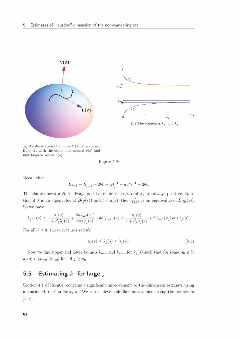
5. Estimates of Hausdorff dimension of the non-wandering set

(a) An illustration of a curve Y (s) on a convexfront X, with the outer unit normal v(s) andunit tangent vector u(s).

(b) The sequences k+j and k−

j .

Figure 5.2:

Recall thatBj+1 = B−

j+1 + 2Θ = (B−1j + djI)

−1 + 2Θ.

The shape operator Bj is always positive definite, so μj and λj are always positive. Notethat if λ is an eigenvalue of B(q(s)) and t < d(x), then λ

1+tλ is an eigenvalue of B(qt(s)).So we have

λj+1(s) ≤λj(s)

1 + djλj(s)+

2κmax(xj)

cosφj(s)and μj+1(s) ≥

μj(s)

1 + djμj(s)+ 2κmin(xj) cosφj(s).

For all j ≥ 0, the curvatures satisfy

μj(s) ≤ kj(s) ≤ λj(s). (5.5)

Now we find upper and lower bounds kmin and kmax for kj(s) such that for some n0 ∈ N,kj(s) ∈ [kmin, kmax] for all j ≥ n0.

5.5 Estimating kj for large j

Section 4.1 of [Ken04] contains a significant improvement to the dimension estimate usinga continued fraction for kj(s). We can achieve a similar improvement using the bounds in(5.5).

54

5.5. Estimating kj for large j

The map fγ,d : (0,∞) → R, x → x1+dx + γ has one positive fixed point g(γ, d) =

γ2 +

√γ2

4 + γd . This function is strictly increasing in γ and strictly decreasing in d, for all

γ, d > 0.The natural domain for g is DN = [2κmin cosφ

+, 2κmaxcosφ+ ]× [d−, d+] for the arguments of g.

On this domain, the minimum and maximum values of g are g(2κmin, d+) and g( 2κmax

cosφ+ , d−)

respectively. While this domain is an obvious choice, it is not the strictest or most usefuldomain. We will use a smaller domain D which we define in Section 5.10. We writekmin = min

(γ,d)∈Dg(γ, d) and kmax = max

(γ,d)∈Dg(γ, d). The values that maximise and minimise g

are denoted (γmax, dmin) and (γmin, dmax) respectively. The numbers dmin and dmax shouldnot be confused with d− and d+. Define sequences k−j and k+j inductively by

k−0 = 0, k−j+1 = fγmin,dmax(k−j ) and

k+0 = k+Sinai, k+j+1 = fγmax,dmin

(k+j ).

Then the sequence kj is bounded by these two sequences, that is for any curve Y ⊂ X, alls ∈ [0, 1] and any j ≥ 0, we have

k−j ≤ μj(s) ≤ kj(s) ≤ λj(s) ≤ k+j .

These sequences have limits

limj→∞

k−j ≥ kmin = g(γmin, dmax) and limj→∞

k+j ≤ kmax = g(γmax, dmin).

Let a < kmin and b > kmax. Then there must be some integer n0 = n(a, b) ≥ 0 such thatfor any convex front X, any curve Y ⊂ X and any s ∈ [0, 1], we have kj(s) ∈ [a, b] for allj ≥ n0. Figure 5.5 illustrates the sequences k−j and k+j .

5.5.1 Estimating δj(s)

Let [a, b] ⊃ [kmin, kmax] and let n0 be defined as above. Define the following constants:

λ−10 = 1 + d+

(1

d−+

2κ+

cosφ+

), μ−1

0 = 1 + 2d−κ− cosφ+,

δ− =1

1 + d+k+Sinai, λ =

1

1 + d+b, and μ =

1

1 + d−a.

Lemma 5.5.1. For any convex front X containing a curve Y : q(s), s ∈ [0, 1], the valuesδj(s) satisfy the following:

• δ0(s) ∈ [δ−, 1],

• δj(s) ∈ [λ0, μ0] for all 1 ≤ j < n0, and

• δj(s) ∈ [λ, μ] for all j ≥ n0.

55

5. Estimates of Hausdorff dimension of the non-wandering set

Proof. Fix an arbitary convex front X containing a curve Y . Now kj(s) ∈ [a, b] for alls ∈ [0, 1] and j > n0. So for j > n0 we have

δj(s) ∈[

1

1 + d+b,

1

1 + d−a

].

For 1 ≤ j < n0 it is easy to see that 2κ− cosφ+ ≤ kj(s) ≤ 1d−+ 2κ+

cosφ+ , so δj(s) ∈ [λ0, μ0].

In the following proposition, we choose a curve Y on a convex front X that is shortenough that its image stays on the same obstacle for several iterations of the billiard ballmap.

Proposition 5.5.2. Fix a point x0 = (q0, v0) ∈ X, a positive integer n and a timeτ ∈ (tm(x0), tm+1(x0)). Let Y : [0, L] → X be a C3 curve with q(0) = q0. Let x(s) =

(q(s), νX(q(s))) and suppose that L > 0 is small enough that for every s ∈ [0, L] we havetm(x(s)) < τ < tm+1(x(s)), and that for all j = 1, . . . , n, s ∈ [0, L] the points qj(s) are onthe same obstacle ∂Kξj . Then p(s) = πSt(x(s)) is a C3 curve on Xt. For all s ∈ [0, 1] wehave

‖q′(s)‖ =‖p′(s)‖

1 + (τ − tm(s))km(s))δ0(s)δ1(s) . . . δm(s).

Proof. See [Sto01, Sto11]. The same result is proved for completeness (but in only twodimensions) in [Ken04].

5.6 Hausdorff dimension of X0

Proposition 5.6.1. Fix an arbitrary convex front X. Let [a, b] ⊃ [kmin, kmax] and n0 =

n(a, b) as defined above. There exist constants c, C depending only on the billiard, such thatfor any integer n ≥ n0 and x1, x2 ∈ X0 such that x1 ≈n x2, we have

cλn−n0 ≤ ‖πx1 − πx2‖ ≤ Cμn−n0 .

Proof. Let n ≥ n0 and let x1, x2 ∈ X0 with x1 ≈n x2. Without loss of generality assumetn(x1) < tn(x2) and let τ = tn(x2). Let y1 = Sτx1, y2 = Sτx2. Now let p(s) parametrize(by arc length) the shortest curve Γ ⊂ SτX between y1 and y2. Let q(s) = S−τ (p(s))

parametrize the curve Y = S−τΓ. This curve will not be the shortest curve on X betweenits endpoints x1 and x2; in fact for large n it can be much longer. We have

‖πx1 − πx2‖ =

∥∥∥∥∫Yq′(s)ds

∥∥∥∥ ≤∫Y‖q′(s)‖ds

=

∫Γ

‖p′(s)‖1 + (τ − tn(s))kn(s)

⎛⎝n−1∏

j=0

δj(s)

⎞⎠ ds

≤ μn−n0μn0−10

∫Γds ≤ Cμn−n0 .

In the second line we use Proposition 5.5.2, and in the third line we use the facts that(τ − tn(s))kn(s) ≥ 0, δj(s) < μ0 for 0 ≤ j ≤ n0, and δj(s) < μ for j > n0. Since the curve Γ

56

5.6. Hausdorff dimension of X0

is the shortest curve between two points on a surface with bounded curvature [Sin70], andconfined to a bounded set (e.g. a ball containing K), its arc length

∫Γ ds can be bounded

above by a constant.Now we find an estimate for ‖x1 − x2‖ from below, using different curves. Let q(s)

parametrise the shortest curve Y in X between x1 and x2. Now let [s1, s2] ⊆ [0, 1] suchthat s = s1, s2 are the only values for which (q(s), n(s)) has an (n+ 1)-th reflection. Lety1 = qn+1(s1), y2 = qn+1(s2). Without loss of generality assume tn+1(s1) < tn+1(s2) andlet τ = tn+1(s1), z = Sτ (q(s2)). Then p(s) = Sτq(s) parametrizes the curve Sτ Y . We haveconstants C1 and C2 such that

‖πx1 − πx2‖ ≥ C1

∫X‖q′(s)‖ds ≥ C1

∫ s2

s1

‖q′(s)‖ds

= C1

∫ s2

s1

‖p′(s)‖1 + (τ − tn(s))kn(s)

⎛⎝n−1∏

j=0

δj(s)

⎞⎠

≥ C1C2δ−λn0−1

0 λn−n0

∫ s2

s1

‖p′(s)‖ds

Clearly z is in the convex hull of the two obstacles containing qn(s2) and y2 respectively,

and y1 is in a third obstacle. Thus we have∫ s2

s1

‖p′(s)‖ ≥ ‖y1 − z‖ ≥ b−, where b− is

the minimum distance between Kk and Cvx (Ki ∪Kj) for any nonequal i, j, k. Lettingc = C1C2λ

n00 b−, we have

cλn−n0 ≤ ‖πx− πy‖ ≤ Cμn−n0

as required.

5.6.1 Representation map

Recall the representation map Υ : X0 → Σ+. Define a metric-specific representation mapbetween metric spaces:

Υθ : (Y0, d) → (Σ+, dθ),

by Υθx = Υx, where d is the Euclidean metric on RD and dθ is the metric defined in

Section 5.4.

Proposition 5.6.2. Let n ≥ n0. Suppose there are constants c, C > 0 such that cλn−n0 ≤‖πx − πy‖ ≤ Cμn−n0 whenever x, y ∈ X0 with x ≈n y. Then Υθ is injective for anyθ ∈ (0, 1). Furthermore, Υλ and Υ−1

μ are both Lipschitz homeomorphisms, but Υ−1λ and Υμ

are not Lipschitz in general.

Proof. For any x ∈ X0 with sufficiently large n ≥ n0, there is some z ∈ X0 such thatz ≈n x, so if Υ(x) = Υ(y) then ‖x − y‖ ≤ ‖x − z‖ + ‖y − z‖ ≤ 2Cμn → 0 as n → ∞.Therefore Υ−1 is well defined, so Υ is injective.

57

5. Estimates of Hausdorff dimension of the non-wandering set

Let x ≈n y ∈ X0. Then dλ(Υλx,Υλy) = λn ≤ 1c‖x−y‖, so Υλ is Lipschitz (and therefore

continuous). For distinct ξ, ξ′ ∈ Υμ(X0), x ∈ Υ−1μ (ξ), y ∈ Υ−1

μ (ξ′), and n such thatx ≈n y ∈ X0, we have ‖Υ−1

μ (ξ)−Υ−1μ (ξ′)‖ ≤ Cμn = Cdμ(ξ, ξ

′), so Υ−1μ is Lipschitz (and

therefore continuous). Since the identity I : (Υθ(X0), dθ) → (Υθ′(X0), dθ′) is continuous,the maps Υθ and Υ−1

θ are continous for any θ, so they are homeomorphisms.

For some ξ ∈ Σ+ and sufficiently large n ≥ n0 the cylinder [ξ]n is a subset of Υ(X0). ByCorollary 4.2.2, the Hausdorff dimensions are related by

dimH Υλ(X0) ≤ dimH X0 ≤ dimH Υμ(X0).

5.7 Hausdorff dimension of M0

We now relate dimH X0 to dimH M0. Let x ∈ M0 and let X = Sτ (W(u)ε (x)) be the image

of the local unstable manifold W(u)ε (x) under St. Let X0 = X ∩M0. From [Sin70], the

curvature of any unstable manifold is bounded above by a constant which we will call k+Sinai.Define D(s) = dimH(W

(s)ε (x) ∩M0) and D(u) = dimH(W

(u)ε (x) ∩M0). Then using Lemma

5.4.1, we get

D(u) = dimH X0 ∈ [− log(u− 1)

log λ,− log(u− 1)

logμ].

We can use the same estimate for D(s), since W(u)ε (x) = Refl(W

(s)ε (Refl(x))), and Refl is

bi-Lipschitz. Recall Theorem 4.2.3: If E,F are Borel sets, then

dimH E + dimH F ≤ dimH(E × F ) ≤ dimH E + dimp F.

Lemma 5.4.1 gives dimp(Σ+, dθ) = dimH(Σ+, dθ) for any θ ∈ (0, 1). Let V be a neigh-

bourhood of M0 and let U ⊂ V be a neighbourhood of x. Let ε be small enough thatW

(u)ε (x),W

(s)ε (x) ⊂ U , and let h : W

(u)ε (x) × W

(s)ε (x) → U be the local product map

defined in Section 4.4.3. This holonomy is at least Hölder continuous. Let ρ be the Hölderconstant of h, then using Proposition 4.2.2 we have

ρ(D(s) +D(u)) ≤ dimH(U ∩M0) ≤ ρ−1(D(s) +D(u)). (5.6)

If ρ ≥ 1 we havedimH(U ∩M0) = D(s) +D(u). (5.7)

Theorem 5.7.1. Let λ1 =1

1+d+kmax, μ1 =

11+d−kmin

. Assume that ρ = 1. Then

−2 log(u− 1)

log λ1≤ dimH M0 ≤

−2 log(u− 1)

logμ1. (5.8)

Proof. For any a < kmin, b > kmax, if λ(b) = 11+d+b

, μ(a) = 11+d−a

we have

dimH M0 = dimH(R ∩M0) = D(s) +D(u) ∈[−2 log(m− 1)

log λ(b),−2 log(m− 1)

logμ(a)

].

Taking the limit as a → kmin and b → kmax, we get the result.

58

5.8. Dimension product structure

5.8 Dimension product structure

In this section we discuss what is currently known about the holonomy h. The holonomy isalways Lipschitz if the diffeomorphism B is conformal on both the stable and unstablemanifolds (see [Bar96] and [Pes97, Chapter 7]). However in dimensions higher than 2, B isnot conformal in general.

However Stoyanov showed in [Sto11] that billiards satisfying a certain geometric propertyalso satisfy a 1/4 pinching condition. When this condition is satisfied the stable andunstable manifolds are C1, and therefore the map h is also C1.

Proposition 5.8.1. [Sto11] A billiard satisfies the 14 -pinching condition if

λd+

0 < μ2d−0 ,

where λ−10 = 1 + d+( 1

d− + 2κ+

cosφ+ ) and μ−10 = 1 + 2d−κ− cosφ+.

In fact we will show that the 14 -pinching condition holds when λ(a)d

+< μ(b)2d

− . Has-selblatt and Schmeling in [HS04] proposed the conjecture that (5.7) holds generically orunder mild hypotheses, even for non-conformal diffeomorphisms and non-Lipschitz localproduct maps. They proved this conjecture for a class of Smale solonoids. If the conjectureis shown to be true, or at least true in the case of dynamical billiards, then we recover (5.8).If not, then the result still holds for the class of billiards in [Sto11]. We now calculate theconstant ρ to get an estimate in terms of constants related to the billiard.

5.9 Calculating the Hölder constant

A combination of techniques from [Sto11, Has94, Has97] and Section 5.10 can be used tocalculate the Hölder constant ρ for the holonomies. The open billiard flow St on M is anexample of an Axiom A flow. Recall the definitions in Section 4.5.3. For any x ∈ M thereexist constants

η(s) < η(s) < 1 < η(u) < η(u),

such that for all vectors u ∈ E(u), v ∈ E(s) and t > 0 we have

1

C

(η(s)

)t‖v‖ ≤ ‖dxSt · v‖ ≤ C

(η(s)

)t‖v‖, and

1

C

(η(u)

)−t‖u‖ ≤ ‖dxS−t · u‖ ≤ C

(η(u)

)−t‖u‖.

For billiards, the reflection property implies that η(u) = (η(s))−1 and η(u) = (η(s))−1. LetX = Sτ (W

(u)ε (x)) for some small τ , let t > d1(x) + . . .+ dn(x) and let δj(s) be defined as

59

5. Estimates of Hausdorff dimension of the non-wandering set

in Section 5.4.3. Then from [Sto11], there are constants c1, c2 such that for all u ∈ E(u),

c1c2

‖u‖δ1(0)δ2(0) . . . δn(0)

≤ ‖dSt(x) · u‖ ≤ c2c1

‖u‖δ1(0)δ2(0) . . . δn(0)

c1c2

‖u‖μn00 μn−n0

≤ ‖dSt(x) · u‖ ≤ c2c1

‖u‖λn00 λn−n0

.

c1c2

(μ

μ0

)n0

μ−t/d+‖u‖ ≤ ‖dSt(x) · u‖ ≤ c2c1

(λ

λ0

)n0

λ−t/d−‖u‖

Aμ−t/d+‖u‖ ≤ ‖dSt(x) · u‖ ≤ Bλ−t/d−‖u‖,

where A = A(a, b) and B = B(a, b) are new global constants that exist for all a < kmin, b >

kmax (these are not necessarily bounded above). This inequality holds for all t ≥ t0 witht0 sufficiently large that m > n0, but there must be constants A′ and B′ such that thesame inequality holds for all 0 < t ≤ t0. Taking C large enough that C > max{B,B′} and1C < min{A,A′}, then we have

η(u) ≤ μ−1/d+ and η(u) ≥ λ−1/d− .

So the bunching constant satisfies

B(B) =2 log η(u)

log η(u)≥ 2d− logμ

d+ log λ.

Recall that the local product map and the stable and unstable manifolds have Hölderconstant at most B(B). This argument improves Proposition 1.2 in [Sto11] by replacing[μ0, λ0] with the smaller interval [μ, λ] for any a < kmin, b > kmax.

Proposition 5.9.1. Let a < kmin, b > kmax. Assume that λ(b)d+

< μ(a)2d− and the

boundary ∂K is C3. Then the open billiard flow in the exterior of K satisfies the pinchingcondition on its non-wandering set M0.

We cannot take the limit as a → kmin, b → kmax for this proposition, since the constantsA and B may not be bounded above. However when λd+ < μ2d− we have ρ ≥ 1 so equations(5.7) and (5.8) hold. Taking limits we can extend this to λd+

1 < μ2d−1 , which proves part 2

of the main theorem. By Corollary 4.5.6 we have that the holonomy h has Hölder constantmin{1, ρ}, where ρ ≥ B(B) ≥ 2d− log μ

d+ log λ. Taking limits as a → kmin, b → kmax, this proves

part 3 of the main theorem.

5.10 Domain of g(γ, d)

Recall that the natural domain for the function g is[2κ− cosφ+,

2κ+

cosφ+

]× [d−, d+].

This domain works well for billiards in RD with D > 2. When D = 2 a more accurate

domain is [2κ−, 2κ+

cosφ+ ]× [d−, d+] (this is the domain used in [Ken04]). To cover both cases

60

5.10. Domain of g(γ, d)

at once, we let ι = 0 if D = 2 and ι = 1 if D > 2, so that cosι φ+ is 1 if D = 2 and cosφ

otherwise. Then the natural domain can be defined

DN =

[2κ− cosι φ+,

2κ+

cosφ+

]× [d−, d+].

However this domain does not take into account differences between the obstacles in K. Itis possible to get more accurate estimates by taking g over a smaller domain. Recall theconstants defined in Section 3.6. Then define the adjusted domain by

D =⋃i,j,k

[2κ−k cosι φ+

ij,k,2κ+k

cosφ+ij,k

]× [d−jk, d

+jk].

The minimum and maximum values of g over the natural domain may be outside of theadjusted domain. The minimum and maximum values in the adjusted domain are given by

kmin = min{g(γ, d) : (γ, d) ∈ D} = min{g(2κ−k cosι φ+ij,k, d

+jk), 1 ≤ i, j, k ≤ u}

kmax = max{g(γ, d) : (γ, d) ∈ D} = max

{g

(2κ+k

cosφ+ij,k

, d−jk

), 1 ≤ i, j, k ≤ u

}

Lemma 5.10.1. For any x = (q, v) ∈ M0, we have(2κ(qk)

cosφk(x), dk(x)

)∈ D and (2κ(qk) cos

ι φk(x)) , dk(x)) ∈ D

for all k ∈ Z.

Proof. Since qk = πBkx ∈ M0 for all k ∈ Z, we have the bounds κ(qk) ∈ [κ−ξk , κ+ξk],

φ(Bkx) ∈ [0, φ+ξk−1ξk+1,ξk

], and d(qk, qk+1) ∈ [d−ξkξk+1, d+ξkξk+1

]. Hence there exist some

integers 1 ≤ i, j,≤ m such that 2κ(qk) cosι φ(Bkx) ≥ 2κ−k cosι φ+ij,k and 2κ(qk)

cosφ(Bkx)≤ 2κ+

k

cosφ+ij,k

.

For the same i, j we have d(xk) ∈ [d−jk, d+jk]. Combining these facts gives the result.

61

5. Estimates of Hausdorff dimension of the non-wandering set

(a) The billiard described in Example 5.10.2.Made using Appendix B, Notebook 2.

(b) The adjusted domain of the billiard in Figure5.10. Made using Appendix B, Notebook 2.

Figure 5.3: Example with three disks.

The following example shows why the adjusted domain is an improvement on the naturaldomain. Two more examples can be found in Chapter 9, and several more can be found inAppendix B, Notebook 2.

Example 5.10.2. Consider the billiard displayed in Figure 5.10 consisting of three disksarranged in an isosceles triangle of height 10 and base length 8. The disks K1,K2,K3 haveradii 1, 2 and 3 respectively. The dots are the period 2 points. Red lines give the distancesd+ij and the purple line segments have length bij,k. Figure 5.10 displays the adjusted domainover the natural domain, with contour lines of the function g(γ, d).

The following estimates were obtained using Mathematica and can be found in AppendixB, Notebook 2. Using the adjusted domain D rather than the natural domain DN meansthat the interval [kmin, kmax] is reduced from [0.760, 7.00] to [0.762, 3.49]. Using the naturaldomain we have the estimate 0.330 ≤ dimH M0 ≤ 1.167, but with the adjusted domain weget 0.394 ≤ dimH M0 ≤ 1.165.

62

Chapter 6

Differentiability of Hausdorffdimension for planar billiards

6.1 Introduction

In this chapter we consider a class of billiards in the plane that are deformed with someparameter α. The deformation could be a translation, rotation, linear transformationor something more complicated. We use the implicit function theorem together withthe periodic points lemma (Lemma 3.3.1) to differentiate the Hausdorff dimension of thenon-wandering set of an open billiard with respect to the parameter α. First, in Section6.2 we define these deformations and establish conditions, for example that the derivativesof a deformation must be bounded. In Section 6.3 we show that the periodic points aredifferentiable with respect to α. In fact we show that the derivatives of each point arebounded by a constant that depends only on geometrical properties of the billiard (minimumand maximum distances, curvatures, and collision angles). In Section 6.6 we extend thisfact to the whole non-wandering set. In Section 6.7 we differentiate the quantities d(x),κ(x), φ(x) and γ(x) = 2κ

cosφ with respect to α, and then use these to differentiate functions

ψ(u)α , ψ

(u)α , which are related to the Lyapunov exponents. Finally in Section 6.8 we use

the dimension theory from Chapter 4 to differentiate the Hausdorff dimension of thenon-wandering set, obtaining the following theorem:

Theorem 6.1.1. (Differentiability of Hausdorff dimension for open billiards)Let K(α) be an open billiard deformation in R

2 with each obstacle parametrized by Cr,r′

functions ϕi(ui, α), with r ≥ 4, r′ ≥ 3, satisfying the conditions in Definition 6.2.1. Let I bean interval in R, then for any α ∈ I, denote the Hausdorff dimension of the non-wanderingset of K(α) by

D(α) = dimH M0.

For any α ∈ I, the function D(α) is Cmin{r−3,r′−1}, and furthermore there exists a constantCψ = Cψ(α), calculated in Section 6.7.3 and depending only on geometric properties of the

63

6. Differentiability of Hausdorff dimension for planar billiards

billiard deformation, such that ∣∣∣∣dD(α)

dα

∣∣∣∣ ≤ CψD(α)

log(1 + d−kmin).

The work in this chapter has been submitted for publication [Wri14a].

6.1.1 Example

To begin, we introduce a simple example of a billiard deformation that we use as motivationfor this chapter.

Example 6.1.2. For any α in the interval [2,∞), let K� = K�(α) = K1 ∪K2 ∪K3(α)

be a billiard consisting of three unit disks with centres arranged in an isosceles trianglewith base 4 and height α. This is sometimes called a Gaspard-Rice system [GR89].Specifically let Ki = B1(ri) where

r1 =

(0

0

), r2 =

(4

0

), r3 =

(2

α

),

and let the boundary of each obstacle be parametrized by functions ϕi(u) = ri +

(cosu

sinu

)

for i = 1, 2, 3. We call this an isosceles deformation. For any α ∈ [2,∞), K�(α) isan open billiard with smooth convex obstacles satisfying the no-eclipse condition. Nowconsider the period 3 orbit ξ = (1, 2, 3). According to Lemma 3.3.1, this corresponds to thesmallest perimeter triangle with points on each ∂Ki. From Corollary 3.3.2, by minimizingthe length function Gξ and then using the implicit function theorem, we obtain threeparameters u1(α), u2(α), u3(α) and three points:

• p1(α) = ϕ1(u1(α)) ∈ ∂K1,

• p2(α) = ϕ2(u2(α)) ∈ ∂K2,

• p3(α) = ϕ3(u3(α), α) ∈ ∂K3.

Figure 6.1 illustrates this deformation with the orbit (1, 2, 3). It is natural to ask how theparameters uj and points pj depend on α.

6.2 Billiard deformations

We want to continuously shift, rotate or otherwise deform the boundary of a billiard andinvestigate the effects on the dimensional characteristics of the system. A deformation willbe described by adding an extra variable α to the parametrisations ϕi, so that any pointon ∂Ki is described by ϕi(ui, α). Denote the perimeter of ∂Ki(α) by Li(α). Then let

Ri = {(ui, α) : α ∈ I, ui ∈ [0, Li(α)]}.

64

6.2. Billiard deformations

Figure 6.1: Isosceles deformation from α to α′ with periodic points corresponding toξ = (1, 2, 3).

Definition 6.2.1. Let I ⊆ [−∞,∞] be a closed interval and let m ≥ 3 be an integer.For any α ∈ I, let K(α) be a subset of R2. For integers r ≥ 2, r′ ≥ 1, we call K(α) aCr,r′-billiard deformation if the following conditions hold for all α ∈ I:

1. K(α) =

m⋃i=1

Ki(α) satisfies the no-eclipse condition (H).

2. Each Ki(α) is a compact, strictly convex set with Cr boundary and total arc lengthLi(α).

3. Each Ki is parametrized counterclockwise by arclength with Cr,r′ functions ϕi : Ri →R2.

4. For all integers 0 ≤ q ≤ r, 0 ≤ q′ ≤ r′ (apart from q = q′ = 0), there exist constantsC

(q,q′)ϕ depending only on α and the parametrizations, such that for all integers

i = 1, . . . ,m, ∣∣∣∣∣ ∂q+q′ϕi

∂uqi∂αq′

∣∣∣∣∣ ≤ C(q,q′)ϕ .

We call α the deformation parameter, and the C(q,q′)ϕ deformation constants. We

assume that only one obstacle is affected by the deformation. This results in strongerestimates for the derivatives. The general case can be covered by considering severalsuccessive deformations, or by deforming several at once (see Remark 6.4.3 for details on

65

6. Differentiability of Hausdorff dimension for planar billiards

this). Define a function δi such that δi = 0 if Ki(α) = Ki is constant for all α, and δi = 1

if Ki(α) depends on α.Since the obstacles are parametrized by arclength, we always have C(1,0) = 1, in fact∣∣∣∂ϕi

∂ui

∣∣∣ = 1. The curvature of ∂K(α) is κi(ui, α) =∣∣∣∂2ϕi

∂u2i

∣∣∣, which is bounded below by κ−

and above by κ+ = C(2,0)ϕ .

6.2.1 Shift maps and billiard expansions

A billiard deformation is called a shift map if Ki(α) = Ki(0)+αv for some constant vectorv. If the deformation is a shift map we can use the parametrization ϕi(u, α) = ϕi(u) + αv

for some function ϕ that parametrises ∂Ki(0). A shift map satisfies C(q,1)ϕ = 0 for all q ≥ 1,

and C(0,1)ϕ = ‖v‖.

For a given billiard K = K1 ∪ . . . ∪ Km, fix a point ri ∈ Ki for each i = 1, . . . ,m. Wecall the deformation a billiard expansion if Ki(α) = Ki + αri for every i. The effect ofthis map is to move all the obstacles apart without changing their shape. These maps areconsidered in the limit α → ∞ in [Ken04].

Example 6.2.2. Let K� be the isosceles deformation from Example 6.1.2. It is easy tosee that K� is a C∞,∞ billiard deformation, specifically a shift map with δ1 = 0, δ2 =

0, δ3 = 1 and v =

(0

1

). We have κ(q) = 1 everywhere, and the following constants:

C(0,1)ϕ = 1, C

(q,0)ϕ = 1 for all q ≥ 1, and all the C(q,q′) = 0 for all other values of q, q′.

Remark 6.2.3. Note that by choosing different parametrisations, we can change thedeformation constants. For example, in the isosceles deformation we could have parametrised∂K3 by

ϕ3(u) =

(cos(u+ α)

α+ sin(u+ α)

).

Even though K3(α) is the same, this is a different billiard deformation with differentdeformation constants: C

(q,q′)ϕ = 2 for q′ = 1 and C

(q,q′)ϕ = 1 otherwise.

6.3 Derivatives of parameters

Let K(α) be a Cr,r′ billiard deformation satisfying the conditions in Definition 6.2.1. Fix afinite admissible sequence ξ = (ξ0, . . . , ξn−1) ∈ Σn. Let

Rξ = {(u, α) : α ∈ I, u = (u0, . . . , un−1), uj ∈ [0, Lξj (α)] for j = 0, . . . , n− 1}.

For each j = 0, . . . , n − 1 set ϕj = ϕξj . By Lemma 3.3.1 and Corollary 3.3.2, thereexist numbers uj(α) = uj(ξ, α) and points pj(α) = pj(ξ, α) = ϕj(uj(α), α) ∈ ∂Kξj whichcorrespond to a billiard trajectory.

66

6.3. Derivatives of parameters

Theorem 6.3.1. Let K(α) be a Cr,r′ billiard deformation, with r ≥ 2, r′ ≥ 1. For anyfinite admissible sequence ξ ∈ Σn, let pj = ϕj(uj(α), α) be the periodic points correspondingto ξ. Then the parameters uj(α) are Cmin{r−1,r′} with respect to the deformation parameterα.

Proof. Fix a sequence ξ with period n. Recall from Chapter 3 that the periodic pointscorresponding to ξ are given by the global minimum of the length function G = Gξ : Rξ → R

defined by

G(u, α) =

n∑j=1

‖ϕj(uj , α)− ϕj−1(uj−1, α)‖.

This is a Cr,r′ function of u and α. We will use the notation Ij = {j − 1, j + 1}. For each j,we can take the partial derivative of G with respect to uj to get the equation

∂G

∂uj(u, α) =

∑i∈Ij

⟨ϕj(uj , α)− ϕi(ui, α)

‖ϕj(uj , α)− ϕi(ui, α)‖,∂ϕj

∂uj(uj , α)

⟩.

By Lemma 3.3.1, for each α ∈ I the function G has a single critical point u = (u1, . . . , un),which satisfies

∂G

∂uj(u(α), α) = 0 for all j = 0, . . . , n− 1.

Now define a function hj : Rj × I → Rn by hj(u, α) =

∂G∂uj

(u, α), and let h be the vector(h0, . . . , hn−1). This is a Cr−1,r′ function of u and α. The Jacobian of h with respect to u

is the Hessian matrix of G:

Hij =∂2G

∂ui∂uj.

This matrix is invertible (see [Sto89]), so we can apply the implicit function theorem.There exists a function u(α) that satisfies h(u(α), α) = 0, and the uj(α) are exactly theparameters that minimize G. So ϕj(uj(α), α), j = 0, . . . , n − 1 are the periodic pointscorresponding to ξ. Furthermore, by Corollary 2.2.6, uj(α) is Cmin{r−1,r′}.

By the implicit function theorem, we have the following system of equations:

∂2G

∂α∂uj(u(α), α) +

n∑i=1

∂ui∂α

∂2G

∂ui∂uj(u(α), α) = 0,

which we can write as a matrix equation,

H∂u

∂α= − ∂

∂α∇G. (6.1)

The next step is to estimate the derivatives ∂uj

∂α .

Theorem 6.3.2. For any ξ ∈ Σn, the derivatives of the parameters satisfy∣∣∣∣∂uj∂α

∣∣∣∣ ≤ 1

cosφj

C(0,1)ϕ + C

(1,1)ϕ d−

κ−d−.

67

6. Differentiability of Hausdorff dimension for planar billiards

Figure 6.2: Demonstration that vjj+1 + vjj−1 = −(2 cosφj)n.

Proof. The two following sections cover the proof of this theorem. We use the notationaij = 1/‖pi − pj‖, vij = aij(pi − pj). Denote by nj the normal vector to ∂K at pj , by κj

the curvature at pj , and by φj = φj(pj , vjj+1) the collision angle. We will use the followingvector identity several times.

Proposition 6.3.3. If u, v, w are unit vectors in the plane, then

〈u,w〉 − 〈v, u〉〈v, w〉 = 〈v, u⊥〉〈v, w⊥〉, (6.2)

where v⊥ is a positive (counterclockwise) rotation by a right angle.

Proof. Let u =

(u1

u2

), v =

(v1

v2

), w =

(w1

w2

)be unit vectors in R

2. Then

〈u,w〉 − 〈v, u〉〈v, w〉 = 〈u,w〉〈v, v〉 − 〈v, u〉〈v, w〉= u2v

21w2 − u2v1v2w1 − u1v1v2w2 + u1v

22w1

= (−u2v1 + u1v2)(−w2v1 + w1v2)

= 〈v, u⊥〉〈v, w⊥〉.

6.3.1 Estimating − ∂∂α∇G

Note that vjj−1 + vjj+1 = −2 cosφjnj where φj is the collision angle at (pj , vjj+1), and nj

is the normal vector of Kξj at φj (see Figure 6.2). We also use the vector identity (6.2).

68

6.3. Derivatives of parameters

∂2G

∂α∂uj=

∂

∂α

∑i∈Ij

⟨ϕj − ϕi

‖ϕj − ϕi‖,∂ϕj

∂uj

⟩

=∑i∈Ij

⟨vji,

∂2ϕj

∂α∂uj

⟩+∑i∈Ij

aji

⟨∂ϕj

∂α− ∂ϕi

∂α,∂ϕj

∂uj

⟩

−∑i∈Ij

aji

⟨vji,

∂ϕj

∂α− ∂ϕi

∂α

⟩⟨vji,

∂ϕj

∂uj

⟩

=∑i∈Ij

aji

⟨vji,

∂ϕj

∂α

⊥− ∂ϕi

∂α

⊥⟩⟨vji,

∂ϕj

∂uj

⊥⟩− 2 cosφj

⟨nj ,

∂2ϕj

∂α∂uj

⟩.

We have⟨vji,

∂ϕj

∂uj

⊥⟩

= cosφj ,∣∣∣∣⟨vji,

∂ϕj

∂α

⊥⟩∣∣∣∣ ≤ δjC

(0,1)ϕ , and

∣∣∣⟨nj ,∂2ϕj

∂uj∂α

⟩∣∣∣ ≤ δjC(1,1)ϕ . We

get the inequality

∣∣∣∣ 1

cosφj

∂2G

∂α∂uj

∣∣∣∣ ≤ C(0,1)ϕ (ajj−1δj−1 + (ajj−1 + ajj+1)δj + ajj+1δj+1) + 2δjC

(1,1)ϕ . (6.3)

Let bj = 1cosφj

∂2G∂α∂uj

. Since only one obstacle is deformed, either δj = 0 or both δj−1 and

δj+1 = 0, so let bmax =2C

(0,1)ϕ

d− + 2C(1,1)ϕ and note that |bj | ≤ bmax for all j.

6.3.2 The Hessian Matrix

The Hessian of G is a matrix composed of the derivatives ∂2G∂uj∂ui

. This section follows[Sto89] and Section 2.2 of [PS92]. The first derivatives of G can be written

∂G

∂uj(u) =

∑i∈Ij

⟨ϕj − ϕi

‖ϕj − ϕi‖,∂ϕj

∂uj

⟩.

If i ∈ Ij , we can use (6.2) to get

∂2G

∂uj∂ui= −aji

⟨∂ϕj

∂uj,∂ϕi

∂ui

⟩+ aji

⟨vji,

∂ϕj

∂uj

⟩⟨vji,

∂ϕi

∂ui

⟩

= −aji

⟨vji,

∂ϕj

∂uj

⊥⟩⟨vji,

∂ϕi

∂ui

⊥⟩

= aji cosφj cosφi.

Along the diagonal i = j we have

∂2G

∂u2j=∑i∈Ij

aji

⟨∂ϕj

∂uj,∂ϕj

∂uj

⟩−∑i∈Ij

aji

⟨vji,

∂ϕj

∂uj

⟩2

+∑i∈Ij

⟨vji,

∂2ϕj

∂u2j

⟩.

Recall that vjj−1+vjj+1 = −(2 cosφj)nj , where nj is the outward unit normal vector. Also

recall that κj =

⟨nj ,

∂2ϕj

∂u2j

⟩. So we have

∑i∈Ij

⟨vji,

∂2ϕj

∂u2j

⟩= 2κj cosφj . Using the vector

identity (6.2) we get

69

6. Differentiability of Hausdorff dimension for planar billiards

∂2G

∂u2j= (ajj−1 + ajj+1) cos

2 φj + 2κj cosφj .

Finally, if i /∈ Ij ∪ {j}, then ∂2G∂uj∂ui

= 0. We will now show the derivatives ∂uj

∂α are bounded.

Proposition 6.3.4. [Sto89] The Hessian matrix H is non-singular and positive definite.

Proof. A proof can be found in [Sto89] or [PS92].

6.4 Solving the cyclic tridiagonal system

From (6.1) and the results of Section 6.3.2, we now have the following system of equations:

∂2G

∂α∂uj= −

n∑i=1

∂ui∂α

∂2G

∂ui∂uj

= ajj−1 cosφj cosφj−1∂uj−1

∂α

+((ajj−1 + ajj+1) cos

2 φj + 2κj cosφj

) ∂uj∂α

+ ajj+1 cosφj cosφj+1∂uj+1

∂α.

For each j, make the substitutions yj =∂uj

∂α cosφj , γj =2κj

cosφjand aj = ajj−1, a1 = an1.

Divide through by cosφj , then we can rearrange the system to

1

cosφj

∂2G

∂α∂uj= ajyj−1 + (aj + aj+1 + γj) yj + aj+1yj+1.

We can write this as a matrix equation Ay = b, where y = (y1, . . . , yn)ᵀ, b = (b1, . . . , bn)

ᵀ,and A is a matrix.⎛

⎜⎜⎜⎜⎜⎜⎜⎝

a1 + a2 + γ1 a2 0 a1

a2 a2 + a3 + γ2 a3 0

a3. . . . . .

0. . . . . . an

a1 0 an an + a1 + γn

⎞⎟⎟⎟⎟⎟⎟⎟⎠

⎛⎜⎜⎜⎜⎜⎜⎜⎜⎝

y1.........yn

⎞⎟⎟⎟⎟⎟⎟⎟⎟⎠

=

⎛⎜⎜⎜⎜⎜⎜⎜⎜⎝

b1.........bn

⎞⎟⎟⎟⎟⎟⎟⎟⎟⎠

.

A tridiagonal matrix only has non-zero elements in the main diagonal and the first diagonalsabove and below the main diagonal. A is cyclic tridiagonal, meaning it can have twomore non-zero elements in the corners. It is also diagonally dominant by rows sinceaj + aj+1 + γj > aj + aj+1 > 0. The problem now is to estimate the solutions yj of thisequation. Here we show three different approaches to solving this problem.

70

6.4. Solving the cyclic tridiagonal system

6.4.1 Estimating the Euclidean norm of y

We can estimate‖y‖2 ≤

‖b‖2σ(A)

≤√nbmax

σ(A),

where σ(A) is the smallest eigenvalue of A. This may seem to be the obvious approach totake. However since

√n is unbounded we cannot use this to find constant bounds on yj

that hold for all n.

6.4.2 Calculating the inverse

Proposition 6.4.1. If n is even, then A−1ij = (−1)i+j |A−1

ij |.

Proof. This is proven in Appendix A.

Assume n is even, then let w = (1,−1, . . . , 1,−1), and

q = Aw = (γ1,−γ2, . . . , γn−1,−γn).

Then for each j we have

wj =∑i

A−1ij qi =

∑i

(−1)i+j |A−1ij |(−1)i+1γi

1 =∑i

|A−1ij |γi ≥ 2κ−

∑i

|A−1ij |

∑i

|A−1ij | ≤ 1

2κ−.

Returning to the system Ay = b we have |yj | ≤ bmax2κ− . Recalling the substitutions we made

earlier, we get ∣∣∣∣∂uj∂α

∣∣∣∣ ≤ 1

cosφj

C(0,1)ϕ + C

(1,1)ϕ d−

κ−d−.

This only applies if n is even. But any periodic orbit ξ of order n is equivalent to aperiodic orbit 2ξ of order 2n, with (2ξ)j = ξj for j = 0, . . . , n − 1 and (2ξ)j = ξj−n forj = n, . . . , 2n− 1, so all orbits are covered by this upper bound. The next approach givesthe same result.

6.4.3 Varah’s Theorem

Let ‖ ‖∞ denote the matrix norm induced by the infinity norm. Recall Varah’s Theorem2.4.9. For our matrix, we have ‖A−1‖∞ ≤ 1

h where

h = mini

((ai + ai+1 + γi)− (ai + ai+1)) = mini

γi ≥ 2κ−.

Returning to the system Ay = b we have ‖y‖∞ ≤ ‖A−1‖∞‖b‖∞, so |yj | ≤ bmax2κ− . Recall that

bmax =2C

(0,1)ϕ

d− + 2C(1,1)ϕ and yj =

∂uj

∂α cosφj . Then we get∣∣∣∣∂uj∂α

∣∣∣∣ ≤ 1

cosφj

C(0,1)ϕ + C

(1,1)ϕ d−

κ−d−.

71

6. Differentiability of Hausdorff dimension for planar billiards

Corollary 6.4.2. Recall that the periodic points p0, . . . , pn−1 are given by pj = ϕj(uj(α), α).So each pj is differentiable with respect to α and we have

dpjdα

=∂ϕj

∂uj

∂uj∂α

+∂ϕj

∂α,

∣∣∣∣dpjdα

∣∣∣∣ ≤ 1

cosφj

C(0,1)ϕ + C

(1,1)ϕ d−

κ−d−+ δξjC

(0,1)ϕ

≤ 1

cosφ+

C(0,1)ϕ + C

(1,1)ϕ d−

κ−d−+ C(0,1)

ϕ ,

where δi = 1 if Ki is affected by the deformation and 0 otherwise.

Following the notation in Section 2.2.3, let

C(1)u =

1

cosφ+

C(0,1)ϕ + C

(1,1)ϕ d−

κ−d−and C(1)

p =1

cosφ+

C(0,1)ϕ + C

(1,1)ϕ d−

κ−d−+ C(0,1)

ϕ (6.4)

Remark 6.4.3. Theorem 6.3.1 assumes that only one obstacle is being deformed. Without

this assumption, we have bmax =4C

(0,1)ϕ

d− +2C(1,1)ϕ instead of 2C

(0,1)ϕ

d− +2C(1,1)ϕ . So the theorem

still holds for deformations of multiple obstacles if we simply replace C(0,1)ϕ +C

(1,1)ϕ d−

κ−d− with2C

(0,1)ϕ +C

(1,1)ϕ d−

κ−d− .

Example 6.4.4. Consider again the isosceles billiard K� from Example 6.1.2, and fix thefinite sequence ξ = (1, 2, 3) = . . . , 1, 2, 3, 1, 2, 3, . . .. We will calculate an upper bound forthe three parameters u1(α), u2(α), u3(α). Recall that C(0,1)

ϕ = 1 and C(1,1)ϕ = 0. From (6.3),

we have ∣∣∣∣ 1

cosφj

∂2G

∂α∂uj

∣∣∣∣ ≤ ajj−1δj−1 + (ajj−1 + ajj+1)δj + ajj+1δj+1 ≤2

d−.

Let bmax = 2d− . Applying the methods in this chapter we obtain a 3×3 matrix A. Applying

Varah’s theorem to A we get

h = mini

γi = mini

2

cosφi.

∣∣∣∣∂uj∂α

∣∣∣∣ ≤ 1

cosφj

bmax

h≤ max

i

cosφi

d− cosφj.

Set α = 3 for example. Then φ1 > φ2 = φ3, so we have∣∣∣∣∂u1∂α

∣∣∣∣ ≤ 1

d−,

∣∣∣∣∂u2∂α

∣∣∣∣ ≤ 1

d−,

∣∣∣∣∂u3∂α

∣∣∣∣ ≤ cosφ2

d− cosφ1.

By inspection, we can see that actually ∂u3∂α = 0. Furthermore it is possible to show

geometrically that∣∣∣∂u1∂α

∣∣∣ is always smaller than 1d− . This agrees with the estimates above.

72

6.5. Higher derivatives of parameters

6.5 Higher derivatives of parameters

Let K(α) be a Cr,r′ billiard deformation, and let k ≤ min{r, r′}. The function hj =∂G∂uj

depends only on {ϕj}j , so all of its derivatives can be estimated as follows:∣∣∣∣∣ ∂q′

∂αq′ ∇qhj

∣∣∣∣∣ ≤ C(q,q′)h ,

where C(q,q′)h is a constant that depends on the constants {C(k,k′)

ϕ }k+k′≤q (but does notdepend on n).

Lemma 6.5.1. Let K(α) be a Cr,r′ billiard deformation and fix a finite admissible sequenceξ ∈ Σn. For every 1 ≤ q ≤ min{r − 1, r′}, there there exists a constant C(q)

u such that∥∥∥∥∂qu

∂αq

∥∥∥∥∞

≤ C(q)u

Proof. We already have the initial case q = 1. For a proof by induction, suppose that forsome q < min{r − 1, r′}, there exist constants C

(1)u , . . . C

(q)u such that∥∥∥∥∂ku

∂αk

∥∥∥∥∞

≤ C(k)u ,

for all k = 1, . . . , q. We show the same is true for q + 1. We need to take the q’th totalderivative of hj(u(α), α) with respect to α. There is a formula known as “Faá di Bruno’sformula” [Arb00], which applies the chain rule for scalar functions an arbitrary number oftimes. In this case, we require a generalization of Faá di Bruno’s formula which applies to ascalar function of a vector function of a scalar. First, write x(α) = (u0(α), . . . , un−1(α), α).Then the formula from [Mis00] can be applied to hj(x(α)). It is a long formula involvingsums over integer partitions, but essentially the total derivative can be written as

dq+1hjdαq+1

(x(α)) =n−1∑j=0

∂2G

∂uj∂ui

∂q+1uj∂αq+1

+P( {

∂k′

∂αk′ ∇khj : k + k′ ≤ q + 1},{

∂luj

∂αl : l ≤ q} )

,

where P is a polynomial over the elements of the two sets. All of the arguments of P canbe estimated by the known constants C(k,k′)

h and C(l)u (k+ k′ ≤ q, l ≤ q), and the inverse of

H is already bounded. So it is possible to calculate a constant C(q+1)u such that∥∥∥∥∂q+1u

∂αq+1

∥∥∥∥∞

≤ C(q+1)u .

So by induction, these estimates exist up to the min{r − 1, r′}’th derivative.

6.6 Extension to aperiodic trajectories

We now consider trajectories in the non-wandering set that are not periodic. Recall thesymbol space Σ, representation map χ and two-sided subshift σ from Section 3.4. For any

73

6. Differentiability of Hausdorff dimension for planar billiards

ξ ∈ Σ and any j ∈ Z, let uj(ξ, α) be the parameter such that pj(ξ, α) = ϕj(uj(ξ, α), α) isthe point πBjχξ. We show that these aperiodic trajectories satisfy the same results as wejust proved for periodic orbits.

Theorem 6.6.1. Let K(α) be a C(r,r′) billiard deformation with r ≥ 2, r′ ≥ 2, and letξ ∈ Σ. Then uj(ξ, α) is C1 with respect to α and∣∣∣∣duj(ξ, α)dα

∣∣∣∣ ≤ C(1)u

where C(1)u is defined by (6.4.1).

Proof. Let ξ ∈ Σ and define a sequence of finite admissible sequences {ξ(n)}n with ξ(n) ∈ Σn,such that ξ(n) → ξ. By Corollary 3.4.4, for any fixed j we have

uj(ξ(n), α) → uj(ξ, α) as n → ∞.

Let fn(α) =ddαuj(ξ

(n), α). This sequence is uniformly bounded for α ∈ I, and so are itsderivatives (by Lemma 6.5.1), so it is equicontinuous. So by the Arzelà-Ascoli theorem(Theorem 2.2.9), it has a uniformly (for α ∈ I) convergent subsequence

fnk(α) =

d

dαuj(ξ

(nk), α).

Let fnk(α) → f(α) as k → ∞. By Proposition 2.2.10, uj(ξ, α) is differentiable with respect

to α, andd

dαuj(ξ, α) = lim

k→∞d

dαuj(ξ

(nk), α).

Then by Theorem 6.3.2, we have ∣∣∣∣duj(ξ, α)dα

∣∣∣∣ ≤ C(1)u .

Corollary 6.6.2. Let K(α) be a C(r,r′) billiard deformation with r, r′ ≥ 2, and let ξ ∈ Σ.Then uj(ξ, α) is Cmin{r−1,r′−1} with respect to α, and all of its derivatives bounded by thesame constants C

(q)u for the periodic trajectories.

Proof. Fix some j ∈ Z. We prove by induction that for all 1 ≤ q ≤ min{r − 1, r′ − 1}, thefunction uj(ξ, α) is Cq, and there exist subsequences

{nq,k}k ⊂ . . . ⊂ {n2,k}k ⊂ {nk}k,

such that the following limit is uniform

limk→∞

dq

dαqu(ξ(nq,k), α) =

dq

dαqu(ξ, α).

The initial case q = 1 is already proven. Suppose it is true for some q ≤ min{r − 2, r′ − 2}.Then the sequence

dq+1u

dαq+1(ξ(nq,k), α)

74

6.7. Derivatives of other billiard properties

is uniformly bounded and equicontinuous for all k (by Lemma 6.5.1), so by the Arzelà-Ascolitheorem it has a uniformly convergent subsequence

dq+1u

dαq+1(ξ(nq+1,k), α).

So by Proposition 2.2.10, u(ξ, α) is Cq+1 and

dq+1

dαq+1u(ξ, α) = lim

n→∞dq+1

dαq+1u(ξ(n), α).

Furthermore ∣∣∣∣∂q+1uj(ξ, α)

dαq+1

∣∣∣∣ ≤ C(q+1)u .

So by induction, u is at least Cmin{r−1,r′−1}.

Remark 6.6.3. The only reason uj(ξ, α) is Cmin{r−1,r′−1} and not necessarily Cmin{r−1,r′}

is the equicontinuity requirement for the Arzelà-Ascoli theorem. It may be possible to showthat uj(ξ, α) is Cmin{r−1,r′} with another method.

Corollary 6.6.4. For all ξ ∈ Σ, the periodic points p(ξ, α) are at least Cmin{r−1,r′−1} withrespect to α, and ∣∣∣∣dp(ξ, α)dα

∣∣∣∣ ≤ Cp.

6.7 Derivatives of other billiard properties

6.7.1 Estimating derivatives of distances, curvatures and collision angles

From here on, let K(α) be a C(r,r′) billiard deformation with r ≥ 4, r′ ≥ 2. We can use theupper bound on ∂uj

∂α to estimate the derivatives of other properties of billiard trajectories,specifically the distances dj , curvature κj and angles φj . We will not estimate the higherderivatives of these functions. Fix a sequence ξ ∈ Σ. The distance function dj(α) isCmin{r−1,r′−1} and we have

dj = |ϕj(uj(α), α)− ϕj−1(uj−1(α), α)|∂dj∂α

≤ ∂ϕj

∂uj

∂uj∂α

+∂ϕj−1

∂uj−1

∂uj−1

∂α+ δj + δj−1

≤ 2C(1,0)ϕ C(1)

u + δξj + δξj−1.

The derivative of κj can also be bounded using the following billiard constant. Recall

that∣∣∣∣∂3ϕj

∂u3j

∣∣∣∣,∣∣∣∣ ∂3ϕj

∂u2j∂α

∣∣∣∣ are bounded above by C(3,0)ϕ and C

(2,1)ϕ respectively. Then κj is

Cmin{r−3,r′−1} and ∣∣∣∣dκjdα

∣∣∣∣ =∣∣∣∣∣∂

3ϕj

∂u3j

∂uj∂α

+∂3ϕj

∂u2j∂α

∣∣∣∣∣≤ C(3,0)

ϕ C(1)u + C(2,1)

ϕ = Cκ.

75

6. Differentiability of Hausdorff dimension for planar billiards

The collision angle φj satisfies cos 2φj =(pj+1−pj)·(pj−1−pj)|pj+1−pj ||pj−1−pj | . Hence, each φj is Cmin{r−1,r′−1}

and we have:

∣∣∣∣d cos 2φj

dα

∣∣∣∣ =∣∣∣∣ pj+1 − pj|pj+1 − pj |

· ∂

∂α

pj−1 − pj|pj−1 − pj |

− pj−1 − pj|pj−1 − pj |

· ∂

∂α

pj+1 − pj|pj+1 − pj |

∣∣∣∣≤ 2

2C(1)u + δξj+1

+ δξj|pj+1 − pj |

+ 22C

(1)u + δξj−1

+ δξj|pj−1 − pj |

≤8C

(1)u + 4δξj + 2δξj+1

+ 2δξj−1

d−,

cosφj =

√cos 2φj + 1

2,

∣∣∣∣d cosφj

dα

∣∣∣∣ ≤ 4C(1)u + 2δξj + δξj+1

+ δξj−1

2d− cosφj.

Denote this upper bound by Cφ (this is a slight departure from the usual notation definedin Section 2.2.3). We will also use the expression γj =

2κj

cosφj. This is Cmin{r−3,r′−1} and we

have ∣∣∣∣∂γj∂α

∣∣∣∣ ≤ 2(C(3,0)ϕ C

(1)u + C

(2,1)ϕ )

cosφj+

2κjcosφj

4C(1)u + 2δξj + δξj−1

+ δξj+1

2d− cos2 φj

≤ 2(C(3,0)ϕ C

(1)u + C

(2,1)ϕ )

cosφ++

2κ+

cosφ+

2C(1)u + 1

d− cos2 φ+.

Denote this upper bound by Cγ .

6.7.2 Stable and unstable manifolds

Definition 6.7.1. Let z = (q, v) ∈ Ω and let z0 be the unique point on M0 such thatStz0 = z for some t ≥ 0. Let X = X(z) ⊂ Ω be the unique convex curve containing q suchthat for any x0 ∈ W

(u)ε (z0), there exists t ≥ 0 and x ∈ X such that St(x0) = (x, νX(x)).

Then X is called a convex front. Then for any x ∈ X(z), define kz(x) to be the curvatureof X(z) at x. If z ∈ M0 and x ∈ W

(u)ε (z), then

kz(x) = limt↓0

kStz(Stx).

X(z) is a Cr curve and the map z → X(z) is at least C1 in general [Sin70, CM06].However if y ∈ X(z) then the curve X(y) overlaps with X(z), so z → X(z) is Cr whenrestricted to these curves. For a fixed z, the map x → kz(x) is Cr−2 since curvature involvesthe second derivative.

Recall that the billiard ball map is an axiom A diffeomorphism, and there exist functionsa(s), a(u) : M0 → R, such that (dxB)v = a(s)(x)Isomxv for all v ∈ E(s) and (dxB)v =

a(u)(x)Isomxv for all v ∈ E(u).

76

6.7. Derivatives of other billiard properties

Proposition 6.7.2. Let K be a planar open billiard. Then the billiard map B is conformalon its stable and unstable manifolds, and

a(u)(x) = 1 + d(x)kx(x), a(s)(x) =1

1 + d(x)kx(x).

Proof. See e.g. Lemma 2.1 of [Sin70], or (3.40) in [CM06].

Note that |a(s)(x)| < 1 and |a(u)(x)| > 1 for all x ∈ M0.

6.7.3 Curvature of unstable manifolds

Definition 6.7.3. For a fixed α ∈ I and ζ ∈ Σ, we have a point z = χ(ζ) and a convexfront X(z). Any point x ∈ X has the same “past” as z, in the sense that B−jz and B−jx

are on the same obstacle for all j ≥ 0. For any ξ ∈ Σ+, let χ+α,ζ(ξ) be the unique point x

on X(z) satisfying Bjx ∈ Kξj for all j ≥ 0.

Fix a sequence ζ ∈ M0 and let z = χ(ζ). Then for any point x ∈ X(z) (sufficiently closeto z), let kj(x) = kBjz(B

jx) be the curvature of the convex front X(Bjz) at Bjx. We havethe following well-known reccurance relation for kj (see e.g. [Sin70, CM06].

kj+1 =kj

1 + djkj+ γj .

This equation is smooth for all dj , kj > 0. Since γj is Cmin{r−3,r′−1}, kj is Cmin{r−3,r′−1}

with respect to α. If x is periodic with period n, then kn = k0 and it is possible to solvethese equations for k0. We can bound kmin ≤ kj ≤ kmax, where kmin, kmax are the constantsdefined in Section 5.5.

Now by writing x = χ+α,ζ(ξ) we can differentiate with respect to α to get

dkj+1

dα=

dkjdα (1 + djkj)− kj(

ddjdα kj + dj

dkjdα )

(1 + djkj)2+

dγjdα

=1

(1 + djkj)2dkjdα

−k2j

(1 + djkj)2ddjdα

+dγjdα

.

Let βj = 1(1+djkj)2

and ηj =dγjdα − k2j

(1+djkj)2ddjdα . We have βj ≤ βmax = 1

(1+d−kmin)2, and

ηj ≤ ηmax = Cγ +k2max(2C

(1)u +1)

(1+d−kmax)2. Then

77

6. Differentiability of Hausdorff dimension for planar billiards

dk0dα

=dkndα

= ηn−1 + βn−1dkn−1

dα

= ηn−1 + βn−1ηn−2 + . . .+ β1 . . . βn−1η0 + β0 . . . βn−1dk0dα

=1

1− β0 . . . βn−1(ηn−1 + βn−1ηn−2 + . . .+ β1 . . . βn−1η0)

≤ 1

1− βnmax

(1 + βmax + . . .+ βn−1

max

)max

jηj

≤ 1

1− βmax

(Cγ +

k2max

(1 + d−kmax)2(2C(1)

u + 1)

)

≤ Ck.

Definition 6.7.4. Fix a sequence ζ ∈ Σ. Define functions ψ(u)α,ζ , ψ

(s)α,ζ : Σ

+ → R as follows:

ψ(u)α,ζ(ξ) = log(1 + d(χ+

α,ζξ)k(χ+α,ζξ)),

ψ(s)α,ζ(ξ) = − log(1 + d(χ+

α,ζξ)k(χ+α,ζξ)).

For a fixed ξ ∈ Σ+, these functions are Cmin{r−3,r′−1} with respect to α, and we have

∣∣∣∣∣∣dψ

(u)α,ζ

dα

∣∣∣∣∣∣ =dd(x)dα k(x) + dk(x)

dα d(x)

1 + d(x)k(x)

≤ Cdk(x) + Ckd(x)

1 + d(x)k(x)

≤ max

{Cdk + Ckd

1 + dk:

k = kmin, kmax,

d = d−, d+

}

≤ Cψ.

Using the reflection property, it is easy to show that ψ(s)α,ζ also satisfies∣∣∣∣∣∣

dψ(s)α,ζ(ξ)

dα

∣∣∣∣∣∣ ≤ Cψ for all ξ ∈ Σ+.

6.7.4 Bounds on Hausdorff dimension

Let D(u) = D(u)(z),D(s) = D(u)(z) be the solution to Bowen’s equations

P (−D(u) log |a(u)|) = 0 and P (D(s) log |a(s)|) = 0.

Let κ(u), κ(s) be the unique equilibrium measures (see Section 4.6.9) corresponding to thefunctions −D(u) log |a(u)|, D(s) log |a(s)|. Now recall Theorem 4.7.1.

1. For any z ∈ M0 and any open set U ⊂ W (u)(z) such that U ∩M0 �= ∅,

dimH(U ∩M0) = dimB(U ∩M0) = dimB(U ∩M0) = D(u).

78

6.7. Derivatives of other billiard properties

2. For any z ∈ M0 and any open set S ⊂ W (s)(z) such that S ∩M0 �= ∅,

dimH(S ∩M0) = dimB(S ∩M0) = dimB(S ∩M0) = D(s).

3. The dimensions of the basic set Λ are given by

dimH(M0) = dimB(M0) = dimB(M0) = D(u) +D(s).

4. The numbers D(u) and D(s) satisfy

D(u) =hκ(u)(f)∫

Λ log |a(u)(x)|dκ(u) and D(s) =hκ(s)(f)∫

Λ log |a(s)(x)|dκ(s) , (6.5)

where hμ(f) is the entropy of f with respect to μ.

Theorem 6.7.5. Let μ0 be the measure such that htop = hμ0. Then the dimension of theunstable manifold satisfies

log(m− 1)∫M0

log |a(u)|dμ0≤ D(u) =

hκ(u)∫M0

log |a(u)|dκ(u) ≤ log(m− 1)∫M0

log |a(u)|dκ(u) .

Proof. By Remark 4.6.5, the topological entropy is

supμ

hμ = htop = log(m− 1).

Since κ(u) is the equilibrium measure for −D(u) log |a(u)|, it satisfies

hκ(u) −D(u)

∫M0

log |a(u)|dκ(u) = supμ

(hμ −D(u)

∫M0

log |a(u)|dμ).

So in particular,

hκ(u) −D(u)

∫M0

log |a(u)|dκ(u) ≥ hμ0 −D(u)

∫M0

log |a(u)|dμ0

0 ≥ htop −D(u)

∫M0

log |a(u)|dμ0

D(u) ≥ log(m− 1)∫M0

log |a(u)|dμ0.

The other inequality is trivial since hκ(u) ≤ htop = log(m− 1).

Theorem 6.7.6. Let μ0 be the measure such that htop = hμ0. Then the dimension of theunstable manifold satisfies

log(m− 1)∫M0

log |a(s)|dμ0≤ D(s) =

hκ(s)∫M0

log |a(s)|dκ(s) ≤ log(m− 1)∫M0

log |a(s)|dκ(s) .

Proof. The proof is very similar to the previous theorem.

79

6. Differentiability of Hausdorff dimension for planar billiards

Corollary 6.7.7. The dimension of the non-wandering set satisfies the estimate given inTheorem 5.2.1 part (i).

Proof. Since the measures κ(u) and μ0 are both ergodic, we have∫M0

dκ(u) =

∫M0

dμ0 = 1.

So

log(1 + d−kmin) ≤∫M0

log(1 + d(x)k(x))dκ(u) =

∫M0

log |a(u)|dκ(u),∫M0

log |a(u)|dμ0 =

∫M0

log(1 + d(x)k(x))dμ0 ≤ log(1 + d+kmax).

The same holds for the stable manifolds, so we have

2 log(m− 1)

log(1 + d+kmax)≤ D(u) +D(s) = dimH M0 ≤

2 log(m− 1)

log(1 + d−kmin)

which is the estimate in Theorem 5.2.1 part (i).

6.8 Derivative of Hausdorff dimension

In this section we show that the Hausdorff dimension of the non-wandering set is differen-tiable with respect to α and that its derivative is bounded by a constant depending onlyon the deformation. We use the definition of topological pressure PΣ+ based on the Ruelleoperator from Section 4.6.7. Recall that for any function ψ : M0 → R, this is related to theclassical topological pressure by

PΣ+(ψ ◦ χ+α,ζ) = Pclassical(B,ψ,M0).

We can rewrite Bowen’s equation using this definition of pressure. The Hausdorff dimensionsD(u) and D(s) are given by

PΣ+(D(u)ψ(u)α,ζ) = PΣ+(D(s)ψ

(s)α,ζ) = 0

We will focus on the unstable manifolds first.

Theorem 6.8.1. Let K(α) be a C(r,r′) billiard deformation with r ≥ 4, r′ ≥ 2. Then theHausdorff dimension D(u) is at least Cmin{r−3,r′−1} with respect to α.

Proof. We will use the implicit function theorem (Theorem 2.2.4) for the following functionof two variables:

Q(D,α) = PΣ+(Dψ(u)α,ζ).

Choose an arbitrary α0 ∈ I, and let D0 ∈ R+ be such that PΣ+(D0ψ

(u)α0,ζ

) = 0. Note

that D0 �= 0 because the entropy is nonzero. Let κ(u)0 be the unique equilibrium measure

corresponding to −D0ψ(u)α0,ζ

. First we show that

∂

∂DQ(D,α)

∣∣∣∣D0,α0

�= 0.

80

6.8. Derivative of Hausdorff dimension

By Proposition 4.6.1, we have

∂

∂DPΣ+

(D0ψ

(u)α0,ζ

+ (D −D0)ψ(u)α0,ζ

)∣∣∣∣D−D0=0

=

∫Σ+

ψ(u)α0,ζ

dκ(u)0 .

By Bowen’s equation and the variational principle we have

0 = P (D0ψ(u)α0,ζ

) = hκ(u)0

+

∫Σ+

D0ψ(u)α0,ζ

dκ(u)0 .

Rearranging this we get

∂

∂DQ(D,α)

∣∣∣∣D0,α0

=

∫Σ+

ψ(u)α0,ζ

dκ(u)0 = −

hκ(u)0

D0.

Since the entropy is never zero in our model, this is non-zero. Since P is analytic, the mapα → P (Dψ

(u)α,ζ) is Cmin{r−3,r′−1} and the map D → P (Dψ

(u)α,ζ) is analytic. So the implicit

function theorem (and its corollary) is applicable. There exists a Cmin{r−3,r′−1} functionD(u)(α), such that P (D(u)(α)ψ

(u)α,ζ) = 0 for all α ∈ I, and furthermore

∂Q

∂α(D(u)(α), α) +

∂D(u)

∂α

∂Q

∂D

(D(u)(α), α

)= 0. (6.6)

Since P (D(u)(α)ψ(u)α,ζ) = 0, the function D(u)(α) is precisely the Hausdorff dimension of

M0 ∩ U for any U ⊂ W (u)(z) with M0 ∩ U �= ∅, for any z = χζ ∈ M0 and any α ∈ I. Thedimension D(u) does not depend on the choice of ζ.

Theorem 6.8.2. Let K(α) be a C(r,r′) billiard deformation with r ≥ 4, r′ ≥ 3. Then ∂D(u)

∂α

is bounded.

Proof. Since r′ ≥ 3, ψ(u)α,ζ is at least C2. So by Corollary 4.6.2, we have

∂

∂αP (D0ψ

(u)α,ζ)

∣∣∣∣α=α0

= D0

∫Σ+

∂ψ(u)α,ζ

∂α

∣∣∣∣∣∣α=α0

dκ(u)0 .

Then (6.6) becomes

0 =∂Q

∂α+

∂D(u)

∂α

∂Q

∂D

∣∣∣∣∣α=α0

= D(u)

∫Σ+

∂ψ(u)α,ζ

∂αdκ

(u)0 − ∂D(u)

∂α

hκ(u)0

D(u)

∣∣∣∣∣∣α=α0

.

Since α0 was chosen arbitrarily, for any α ∈ I we have

∂D(u)

∂α=

D(u)(α)2

hκ(u)

∫Σ+

∂ψ(u)α,ζ

∂αdκ(u). (6.7)

The integrand is bounded by Cψ, and κ(u) is a probability measure, so we have∣∣∣∣∣∂D(u)

∂α

∣∣∣∣∣ ≤ D(u)(α)2

hκ(u)

Cψ.

81

6. Differentiability of Hausdorff dimension for planar billiards

Theorem 6.8.3. Let K(α) be a Cr,r′ billiard deformation with r ≥ 4, r′ ≥ 3. For anysequence ζ, the Hausdorff dimension D(s) of M0 ∩W (s)(χz) is at least Cmin{r−3,r′−1} withrespect to α, and its first derivative is bounded by

D(s)(α)2Cψ

hκ(s)

.

Proof. By the reflection property W(u)ε (z) = ReflW (s)

ε (Refl(z)), we have

ψ(s)α,ζ = −ψ

(u)α,ζ and D(s) = D(u).

So the proof is very similar to the previous theorem.

Theorem 6.8.4. Let K(α) be a Cr,r′ billiard deformation with r ≥ 4, r′ ≥ 3. The Hausdorffdimension D(α) = D(u) +D(s) of the non-wandering set is Cmin{r−3,r′−1} with respect to α,and its derivative is bounded by the following.∣∣∣∣dDdα

∣∣∣∣ ≤ CψDlog(1 + d−kmin)

.

Proof. Since B is conformal, the dimension satisfies D(α) = D(s)(α) +D(u)(α). So∣∣∣∣dDdα∣∣∣∣ ≤ D(s)(α)2Cψ

hκ(s)

+D(u)(α)2Cψ

hκ(u)

≤ CψD(s)(α)

log(1 + d−kmin)+

CψD(u)(α)

log(1 + d−kmin)

≤ CψD(α)

log(1 + d−kmin).

This follows from the final part of Theorem 4.7.1.

Remark 6.8.5. Note that r′ ≥ 3 is only required for estimating the first derivative. Tofind the differentiability class of the Hausdorff dimension only r′ ≥ 2 is required.

Corollary 6.8.6. Let K(α) be a real analytic billiard deformation (i.e. real analytic inboth α and the parameter u). Then D(α) is a real analytic function of α.

Proof. Let K(α) be a real analytic billiard deformation. Then clearly the functions F ,G and h are all real analytic. By the implicit function theorem for analytic functions(Corollary 2.2.5), uj(ξ, α) is real analytic for any periodic admissible sequence ξ. To extendthis to aperiodic sequences, we show that uj(ξ, α) is equal to its Taylor series at any pointα0 and for any ξ ∈ Σ. Recall from the proof of Corollary 6.6.2 that for each q there existsa sequence (ξ(nq,k))k such that lim

k→∞ξ(nq,k) = ξ, and

dq

dαquj(ξ, α) = lim

k→∞dq

dαquj(ξ

(nq,k), α).

82

6.8. Derivative of Hausdorff dimension

Now using the definition of real analyticity, we have

uj(ξ, α) = limk→∞

uj(ξ(nq,k), α)

= limk→∞

∞∑q=0

(α− α0)q

q!

(dq

dαquj(ξ

(nq,k), α)

∣∣∣∣α=α0

)

=

∞∑q=0

(α− α0)q

q!

(limk→∞

dq

dαquj(ξ

(nq,k), α)

∣∣∣∣α=α0

)

=∞∑q=0

(α− α0)q

q!

(dq

dαquj(ξ, α)

∣∣∣∣α=α0

).

Therefore uj(ξ, α) is real analytic in α. Now the quantities p, d, κ, φ and γ are all easilyshown to be real analytic. The recurrance relation for kj can be used to show that kj isreal analytic, and therefore ψα,ζ(ξ) is real analytic. Since the pressure is a real analyticoperator, it follows that D(α) is real analytic.

83

Chapter 7

Differentiability of Hausdorffdimension for nonplanar billiards

7.1 Introduction

In this chapter we investigate deformations of billiards in RD for D ≥ 3 and replicate some

of the results in Chapter 6. Since the billiard map in dimensions higher than two is notconformal, Bowen’s equation is replaced by inequalities, and there is currently no knownequation for the Hausdorff dimension of the non-wandering set. So we will not be able toshow continuity or estimate the derivatives of the Hausdorff dimension. However we canstill differentiate the points of the non-wandering set and the functions ψ

(u)α,ζ with respect

to deformations of the boundary.

7.1.1 Notation

We will be using block vectors and block matrices in this chapter (see Section 2.4.1).For block vectors u = (u10, . . . , u

D−10 ; . . . ;u1n−1, . . . , u

D−1n−1 ) we define the following sets of

operators:

∇qj =

⎧⎨⎩ ∂q∏D−1

t=1 ∂(utj)qt

: qt ∈ {0, . . . , q},n∑

j=1

qt = q

⎫⎬⎭ ,

and

∇q =

⎧⎨⎩ ∂q∏n−1

j=0

∏D−1t=1 (∂utj)

qj,t: qj,t ∈ {0, . . . , q},

n−1∑j=0

D−1∑t=1

qj,t = q

⎫⎬⎭ .

7.2 Billiard deformations in higher dimensions

Recall the concept of orthonormal parametrisation from Section 3.2.

85

7. Differentiability of Hausdorff dimension for nonplanar billiards

Definition 7.2.1. Let I ⊆ [−∞,∞] be a closed interval and let D ≥ 3, m ≥ 3 be integers.For any α ∈ I, let K(α) be a subset of RD. For integers r ≥ 2, r′ ≥ 1, we call K(α) aCr,r′-billiard deformation if the following conditions hold.

1. K(α) =

m⋃i=1

Ki(α) defines an open billiard in RD satisfying the no-eclipse condition

(H).

2. Each Ki(α) is a compact, strictly convex set with Cr boundary.

3. For each i = 1, . . . ,m and all p ∈ ∂Ki(α), there exists a rectangle Rp(α) ⊂ RD−1 and

a C(r,r′)-smooth function ϕp : Rp → RD, which is an orthonormal parametrisation of

∂Ki(α) at p.

4. For all integers 0 ≤ q ≤ r, 0 ≤ q′ ≤ r′ (apart from q = q′ = 0), and for all α ∈ I,there exist constants C(q,q′)

ϕ depending only on α and the parametrizations, such thatfor all integers i = 1, . . . ,m, ∣∣∣∣∣ ∂

q′

∂αq′ ∇qi ϕi

∣∣∣∣∣ ≤ C(q,q′)ϕ .

We call α the deformation parameter, and the C(q,q′)ϕ deformation constants. Note

that since each parametrisation ϕp is orthonomal at pj , we have C(1,0)ϕ = 1. We assume that

only one obstacle is affected by the deformation. This results in stronger estimates for thederivatives. The general case can be covered by considering several successive deformations,or by deforming several at once (see Section 7.4.1 for details on this).

Example 7.2.2. We consider a billiard deformation consisting of moving spheres. Forsome interval I and any α ∈ I, let vi be a unit vector, let ai(α) = ai + αv, and let ri > 0

for i = 1, . . . ,m and let Ki = Bri(ai). Assume that K(α) =⋃m

i=1Ki satisfies the no-eclipsecondition for all α ∈ I. We can parametrize the obstacles with the techniques in Example3.2.2. Then we have curvatures κ− = κ+ = 1, C(0,1)

ϕ = ‖v‖, C(q,0)ϕ = 1 for all q ≥ 1 and

C(q,q′)ϕ = 0 for all other values of q, q′.

7.3 Derivatives of parameters

Let K(α) be a Cr,r′ billiard deformation satisfying the conditions in Definition 6.2.1. Fix afinite admissible sequence ξ = (ξ0, . . . , ξn−1) ∈ Σn. By Lemma 3.3.1, for j = 0, . . . , n− 1

there exist points pj(α) ∈ ∂Kξj that correspond to a billiard trajectory. Let ϕj(uj , α) =

ϕpj(α)(uj); this is an orthonormal parametrisation of ∂Kξj .By Corollary 3.3.2, there exist uj(α) = uj(ξ, α) ∈ Rj that satisfy pj(α) = ϕj(uj(α), α).

Set u(α) = (u0, . . . , un−1). This is a block vector (see Section 2.4.1) Let

Rξ = {(u, α) : α ∈ I, u = (u0, . . . , un−1), uj ∈ Rpj (α) for j = 0, . . . , n− 1}.

86

7.3. Derivatives of parameters

Theorem 7.3.1. Let K(α) be a Cr,r′ billiard deformation, with r ≥ 2, r′ ≥ 1. For anyfinite admissible sequence ξ ∈ Σn, let pj = ϕj(uj(α), α) be the periodic points correspondingto ξ. Then the parameters uj(α) are Cmin{r−1,r′} with respect to the deformation parameterα.

Proof. Fix a sequence ξ with period n. Let Ij = {j − 1, j + 1}. Recall that the uj(α) aregiven by the global minimum of the length function Gξ : Rξ → R defined by

G(u, α) =n∑

j=1

‖ϕj(u, α)− ϕj−1(u, α)‖.

This is a Cr,r′ function of u and α. For each j, we can take the partial derivative of G withrespect to uj to get the equation

∂G

∂utj(u, α) =

∑i∈Ij

⟨ϕj(uj , α)− ϕi(ui, α)

‖ϕj(uj , α)− ϕi(ui, α)‖,∂ϕj

∂utj(uj , α)

⟩.

By Lemma 3.3.1, for each α ∈ I the function G has a single critical point u = (u1, . . . , un),which satisfies

∂G

∂utj(u(α), α) = 0 for all j = 0, . . . , n− 1 and t = 1, . . . , D − 1.

Now define a function htj : Rj × I → Rn by htj(u, α) =

∂G∂ut

j(u, α), and let h be the block

vector (h10, . . . , hD−10 ; . . . ;h1n−1, . . . , h

D−1n−1 ). This is a Cr−1,r′ function of u and α. The

Jacobian of h with respect to u is the Hessian matrix of G:

Htsij =

∂2G

∂uti∂usj

.

This matrix is invertible (see [Sto89]), so we can apply the implicit function theorem.There exists a function u(α) that satisfies h(u(α), α) = 0, and the uj(α) are exactly theparameters that minimize G. So ϕj(uj(α), α) is the j’th periodic points corresponding toξ. Furthermore, by the generalized implicit function theorem (Corollary 2.2.6), uj(α) isCmin{r−1,r′}.

From the implicit function theorem, we have

dhtjdα

=∂

∂α

∂G

∂utj(u(α), α) +

n∑i=1

n∑s=1

∂usi∂α

∂2G

∂uti∂usj

(u(α), α) = 0.

We can write this as a matrix equation,

H∂u∂α

= − ∂

∂α∇G, (7.1)

where ∇ is the block vector {∇1, . . . ,∇n} = { ∂∂u1

1, . . . , ∂

∂ud1; . . . ; ∂

∂u1n, . . . , ∂

∂udn}. The next

step is to estimate the derivatives ∂uj

∂α .

87

7. Differentiability of Hausdorff dimension for nonplanar billiards

Theorem 7.3.2. For any ξ ∈ Σn, the derivatives of the parameters satisfy∣∣∣∣∂uj∂α

∣∣∣∣ ≤ 1

cosφj

C(0,1)ϕ + C

(1,1)ϕ d−

κ−d−.

The rest of this section concerns the proof of this theorem. We use the following notation:Let aji = 1/‖pj − pi‖, vji = aji(pj − pi). Denote by nj = n∂K(pj) the normal vectorat pj , by κ

(t)j = κ

(t)∂K(pj) the t’th principle curvature at pj for t = 1, . . . , D − 1, and by

φj = φ(pj , vjj+1) the collision angle at pj .Let Uj = Upj be the D × D − 1 matrix of derivatives ∂ϕj

∂uj, and let Wj = Wpj be the

D ×D matrix with the first D − 1 columns the same as Uj and the last column given bynj = n∂K(pj). This is an orthogonal matrix because ϕpj is orthonormal at pj . Let IIj = IIpjbe the second fundamental form of ∂Kξj at pj . Let U denote the nD × n(D − 1) blockmatrix with Uj down the diagonals, and rectangular zero matrices at the other positions.Let W denote the nD × nD block diagonal matrix with Wj at the j’th block.

We will use the following vector identity several times.

Proposition 7.3.3. If v is a unit vector and u,w are vectors, then

〈w, u〉 − 〈v, w〉〈v, u〉 = (uᵀw)(vᵀv)− (uᵀv)(vᵀw) = uᵀ(I − vvᵀ)w (7.2)

This is a more general statement than the vector identity 6.3.3.

7.3.1 Calculating − ∂∂α∇G

For any i = 1, . . . n, define a function δi such that δi = 0 if Ki(α) = Ki is constant for allα, and δi = 1 if Ki(α) depends on α. Note that vjj−1 + vjj+1 = −2 cosφjnj .

∂2G

∂α∂utj=

∂

∂α

∑i∈Ij

⟨ϕj − ϕi

‖ϕj − ϕi‖,∂ϕj

∂utj

⟩

=∑i∈Ij

⟨vji,

∂2ϕj

∂α∂utj

⟩+∑i∈Ij

aji

⟨∂ϕj

∂α− ∂ϕi

∂α,∂ϕj

∂utj

⟩

−∑i∈Ij

aji

⟨vji,

∂ϕj

∂α− ∂ϕi

∂α

⟩⟨vji,

∂ϕj

∂utj

⟩

= −2 cosφj

⟨nj ,

∂2ϕj

∂α∂utj

⟩+∑i∈Ij

aji∂ϕj

∂utj

ᵀ (I − vjiv

ᵀji

)(∂ϕj

∂α− ∂ϕi

∂α

).

Let Vji = aji(I − vjivᵀji). This is is a symmetric, singular, d× d matrix with eigenvalues

0 (multiplicity 1) and aji (multiplicity d− 1). Recall from Definition 3.2.1 that Uj is therectangular matrix of derivatives of ϕj . Then we can write the above equation in matrixform:

− ∂

∂α∇jG = 2nᵀ

j

∂Uj

∂αcosφj −

∑i∈Ij

Uᵀj Vji

(∂ϕj

∂α− ∂ϕi

∂α

). (7.3)

88

7.3. Derivatives of parameters

Now notice that the vectors in ∂Uj

∂α have magnitude less than C(1,1)ϕ , the vectors in Uj and

Vj have magnitude equal to or less than 1, and the magnitude of each ∂ϕi

∂α is bounded byC

(0,1)ϕ . So we have∣∣∣∣∣ ∂2G

∂α∂utj

∣∣∣∣∣ ≤ 2C(1,1)ϕ + (δj−1ajj−1 + δj(ajj−1 + ajj+1) + δj+1ajj+1)C

(0,1)ϕ .

Let C(1,1)G = 2C

(1,1)ϕ +

2C(0,1)ϕ

dmin. Then we can say

∥∥∥∥− ∂

∂α∇G

∥∥∥∥∞

≤ C(1,1)G . (7.4)

7.3.2 Hessian matrix

Note that vjj−1 + vjj+1 = −(2 cosφj)nj , where nj is the outward unit normal vector. Sowe have ∑

i∈Ij

⟨vji,

∂2ϕj

∂usj∂utj

⟩= 2 cosφj

⟨nj ,

∂2ϕj

∂usj∂utj

⟩= 2IIstj cosφj ,

where IIj is the matrix representing the second fundamental form of ϕj at qj . Along thediagonal i = j and for any 1 ≤ s, t ≤ D − 1, we have

∂2G

∂usj∂utj

=∑i∈Ij

aji

⟨∂ϕj

∂usj,∂ϕj

∂utj

⟩−∑i∈Ij

aji

⟨vji,

∂ϕj

∂usj

⟩⟨vji,

∂ϕj

∂utj

⟩

+∑i∈Ij

⟨vji,

∂2ϕj

∂usj∂utj

⟩

=∑i∈Ij

aji

(∂ϕj

∂usj

)ᵀ (I − vjiv

ᵀji

) ∂ϕj

∂utj+ 2IIstj cosφj .

So the diagonal blocks of the Hessian matrix are given by

Hjj =∑i∈Ij

Uᵀj VjiUj + 2IIj cosφj .

On the subdiagonal or superdiagonal lines, i ∈ Ij , 1 ≤ s, t ≤ d− 1, we have

∂2G

∂usj∂uti= −aji

⟨∂ϕj

∂usj,∂ϕj

∂utj

⟩+ aji

⟨vji,

∂ϕj

∂usj

⟩⟨vji,

∂ϕi

∂uti

⟩

= −aji

(∂ϕj

∂usj

)ᵀ (I − vjiv

ᵀji

) ∂ϕi

∂uti.

So the subdiagonal and superdiagonal blocks of the Hessian matrix are given by

Hij = Uᵀj VjiUi.

Finally, if i /∈ Ij ∪ j, then Hij =∂2G

∂uj∂ui= O, where O is the d× d zero matrix.

89

7. Differentiability of Hausdorff dimension for nonplanar billiards

7.4 System of matrix equations

Let Vj = Vjj−1 = ajj−1(I − vjj−1vᵀjj−1). We want to process everything as one large block

matrix equation. But the situation at the moment is a system of matrix equations thatinvolves D×D square matrices Vj , D×D− 1 rectangular matrices Uj , and D− 1×D− 1

matrices IIj . To resolve this problem, we introduce extra rows and columns to the smallermatrices. Recall that Wj is a square matrix with the columns of Uj in the first D − 1

columns and nj in the final column. For each j, define a D ×D matrix Kj by

Kj = 2 cosφjW−ᵀj

(IIj 00ᵀ C

)W−1

j ,

where 0 is the zero vector in Rd−1 and C ∈ (σ(IIj), ‖IIj‖) is an arbitrary constant between

the smallest and largest singular values of IIj . This requirement is just so that the thevalues of ‖Kj‖ and σ(Kj) do not depend on C. However apart from this condition, theconstant C will drop out of future equations and never be used.

Then Kj is a D × D matrix and Uᵀj KjUj = 2IIj cosφj . Since Wj is orthogonal, the

eigenvalues of Kj are 2C cosφj , followed by the eigenvalues of IIj multiplied by 2 cosφj . Sowe have

2κ−j cosφj ≤ σ(Kj) ≤ ‖Kj‖ ≤ 2κ+j .

We have the following system of matrix equations:

− ∂2G

∂α∂uj=− Uᵀ

j VjUj−1∂uj−1

∂α

+(Uᵀj KjUj + Uᵀ

j VjUj + Uᵀj Vj+1Uj

) ∂uj∂α

− Uᵀj Vj+1Uj+1

∂uj+1

∂α.

Now make the following substitutions:

bj = W−ᵀj

(∂2G

∂α∂u1j

. . . ∂2G∂α∂ud−1

j

0)ᵀ

,

yj = Wj

(∂u1

j

∂α . . .∂ud−1

j

∂α 0

)ᵀ.

Then the system becomes

bj = −Vjyj−1 + (Kj + Vj + Vj+1) yj − Vj+1yj+1.

We can write this as a single matrix equation Ay = (K + V)y = b, where b is the blockvector of bj ’s, K is a block matrix with Kj along the diagonal, and V is the nd×nd matrix

V =

⎛⎜⎜⎜⎜⎜⎜⎜⎝

V1 + V2 −V2 −V1

−V2 V2 + V3 −V3

. . . . . . . . .

−Vn−1 Vn−1 + Vn −Vn

−V1 −Vn Vn + V1

⎞⎟⎟⎟⎟⎟⎟⎟⎠

.

90

7.4. System of matrix equations

Since Wj is orthogonal we have ‖Wj‖2 = 1, so

‖bj‖2 =∥∥∥∥ ∂

∂α∇jG

∥∥∥∥2

≤√D

((δj−1 + 2δj + δj+1)

c1dmin

+ 2c2 cosφ

),∣∣∣∣∣∂u

tj

∂α

∣∣∣∣∣ ≤√D‖yj‖2.

Now we use the concept of block norms from Chapter 2. Recall Theorem 2.4.11 (Varah’stheorem for weakly block diagonally dominant matrices). We have σ(Vj) = 0 and σ(Kj) ≥2κ− cosφ+, where κ− is the smallest of the principle curvatures of any of the obstacles.Since Ki and Vi are positive definite, we have σ(Aii) ≥ σ(Ki) + σ(Vi) + σ(Vi+1). So A isweakly diagonally dominant. By Theorem 2.4.11, we have

‖A−1‖∞,2 ≤1

h,

where

h = mini

⎛⎝σ(Aii)−

∑j �=i

σ(Aij)

⎞⎠ ≥ 2κ− cosφ+.

Now we need to relate the block matrix norm to the infinity norm. It is easy to showthat for vectors, these norms are equivalent up to the constant

√D, that is, for any vector

x ∈ RnD,

1√D‖x‖∞ ≤ ‖x‖∞,2 ≤

√D‖x‖∞.

So we have

‖A−1‖∞ = maxx �=0

‖Ax‖∞‖x‖∞

≤ maxx �=0

√D‖A‖∞,2‖x‖∞,2

‖x‖∞≤ D

2κ− cosφ+.

Now we can estimate the derivatives of the parameters uj :

∣∣∣∣∣∂utj

∂α

∣∣∣∣∣ ≤ D‖A−1‖∞,2 ‖b‖∞

≤ D

2κ− cosφ+

(2C(1,1)

ϕ +2C

(0,1)ϕ

d−

).

Let Cu = D2κ− cosφ+

(2C

(0,1)ϕ

d− + 2C(1,1)ϕ cosφ+

).

Recall that the periodic points p = (p1, . . . , pn) are given by pj = ϕj(uj(α), α). So eachpj is differentiable with respect to α and we have

dpjdα

= Uᵀj

∂uj∂α

+∂ϕj

∂α.

91

7. Differentiability of Hausdorff dimension for nonplanar billiards

As a block matrix equation, this is

dpdα

= Uᵀ ∂u∂α

+∂ϕ

∂α,

where ϕ is the block vector (ϕ1, . . . , ϕn−1). There are two ways to estimate the derivativesof the points. Using the estimation for

∣∣∣∂utj

∂α

∣∣∣ we get

∣∣∣∣dpjdα

∣∣∣∣ ≤ D

2κ− cosφ+

(2C

(0,1)ϕ

d−+ 2C(1,1)

ϕ cosφ+

)+ δj .

Alternatively, let m be the block vector mj = 2 cosφj∂Uᵀ

j

∂α nj . Then we can rewrite (7.3) inblock matrix form:

− ∂

∂α∇G = m − UᵀV

∂ϕ

∂α. (7.5)

Now combine (7.1) and (7.5) to get

Uᵀ(V + K)U∂u∂α

= m − UᵀV∂ϕ

∂α. (7.6)

Add Uᵀ(V + K)∂ϕ∂α to each side to get

Uᵀ(V + K)

(U∂u∂α

+∂ϕ

∂α

)= m + UᵀK

∂ϕ

∂α∥∥∥∥∂p∂α∥∥∥∥∞,2

≤ ‖W−ᵀ‖‖A−1‖∞,2

∥∥∥∥m + UᵀK∂ϕ

∂α

∥∥∥∥∞,2∥∥∥∥dpjdα

∥∥∥∥∞

≤ D

2κ− cosφ+(2C(1,1)

ϕ + κ+C(0,1)ϕ δj)

We can use either estimate. So let

Cp =D

2κ− cosφ+

(2C(1,1)

ϕ + C(0,1)ϕ min

{4

d−, κ+

}).

Then ∣∣∣∣dpjdα

∣∣∣∣ ≤ Cp.

Remark 7.4.1. This theorem assumes that only one obstacle is being deformed. Without

this assumption, we have bmax = 2C(1,1)ϕ +

4C(0,1)ϕ

dmininstead of 2C(1,1)

ϕ +2C

(0,1)ϕ

d− . So the theorem

still holds for deformations of multiple obstacles if we simply replace C(0,1)ϕ +C

(1,1)ϕ d−

κ−d− with2C

(0,1)ϕ +C

(1,1)ϕ d−

κ−d− .

7.5 Higher derivatives of parameters

Let K(α) be a Cr,r′ billiard deformation, and let k ≤ min{r, r′}. The function hj =∂G∂uj

depends only on {ϕj}j , so all of its derivatives can be estimated as follows∣∣∣∣∣ ∂q′

∂αq′ ∇qhj

∣∣∣∣∣ ≤ C(q,q′)h ,

92

7.6. Extension to aperiodic trajectories

where C(q,q′)h is a constant that depends on the known constants {C(k,k′)

ϕ }k≤q,k′≤q′ (butdoes not depend on n).

Lemma 7.5.1. Let K(α) be a Cr,r′ billiard deformation and fix a finite admissible sequenceξ ∈ Σn. For every q ≤ min{r − 1, r′}, there there exists a constant Cq

u such that∥∥∥∥∂qu∂αq

∥∥∥∥∞

≤ C(q)u

Proof. We already have the initial case q = 0. Suppose that for some q < min{r − 1, r′},there exist constants C

(1)u , . . . C

(q)u such that∥∥∥∥∂ku

∂αk

∥∥∥∥∞

≤ C(k)u ,

for all k = 1, . . . , q. We show the same is true for q + 1. We need to take the q + 1’th totalderivative of htj(u(α), α) with respect to α. First, write

x(α) = (u10(α), . . . , uD−10 (α), . . . , u1n−1, . . . u

D−1n−1 (α), α).

Then the formula from [Mis00] can be applied to htj(x(α)). The q’th total derivative canbe written as the following

dq+1htjdαq+1

=

n−1∑j=0

∂2G

∂uj∂ui

∂q+1utj∂αq+1

+ P

⎛⎜⎝{ ∂k

∂αk′ ∇qhtj : k + k′ ≤ q + 1

},

⎧⎪⎨⎪⎩∂lusi∂αl

:

0 ≤ i ≤ n− 1,

1 ≤ s ≤ D − 1,

1 ≤ l ≤ q

⎫⎪⎬⎪⎭⎞⎟⎠ .

where P is a polynomial over the elements of the sets. All of the arguments of P can beestimated by the known constants C

(k,k′)h and C

(l)u (k + k′ ≤ q, l ≤ q), and the inverse of H

is already bounded. So it is possible to calculate a constant C(q+1)u such that∥∥∥∥∂q+1u

∂αq+1

∥∥∥∥∞

≤ C(q+1)u .

So by induction, these estimates exist up to the min{r − 1, r′}’th derivative.

7.6 Extension to aperiodic trajectories

We now consider trajectories in the non-wandering set that are not periodic. Recall thesymbol space Σ, representation map χ and two-sided subshift σ from Section 3.4. For anyξ ∈ Σ and any j ∈ Z, let uj(ξ, α) be the parameter such that pj(ξ, α) = ϕξj (uj(ξ, α), α) isthe point πBjχαξ. These aperiodic trajectories satisfy the same results as we just provedfor periodic orbits.

93

7. Differentiability of Hausdorff dimension for nonplanar billiards

Theorem 7.6.1. Let K(α) be a C(r,r′) billiard deformation with r, r′ ≥ 2, and let ξ ∈ Σ.Then uj(ξ, α) is Cmin{r−1,r′−1} with respect to α, and all of its derivatives bounded by thesame constants C

(q)u as for the periodic trajectories.

Proof. The proof of this is identical to the proof of Theorem 6.6.1 and Corollary 6.6.2

7.7 Derivatives of distances, curvatures, collision angles and

convex fronts

Here we fix a sequence ξ and differentiate various quantities associated with ξ, just as wedid in the plane in Section 6.7.

7.7.1 Estimating derivatives of distances, curvatures and collision angles

Let ξ ∈ Σ. We can use the upper bounds on ∂uj

∂α and ∂pj∂α to estimate the derivatives of

other properties of billiard trajectories, specifically the distances dj , principal curvaturesκtj and collision angles φj . The distance function dj(α) is Cmin{r−1,r′−1}, and satisfies

dj = |ϕj(uj(α))− ϕj−1(uj−1(α))|∣∣∣∣∂dj∂α

∣∣∣∣ ≤ ∂ϕj

∂uj

∂uj∂α

+∂ϕj−1

∂uj−1

∂uj−1

∂α+ δj + δj−1

≤ 2Cu + 1.

Alternatively we can simply estimate∣∣∣∂dj∂α

∣∣∣ ≤ 2Cp. Choose the smaller estimate and call it

Cd. The unit velocity vectors can also be differentiated, and we get∣∣∣∂vji∂α

∣∣∣ ≤ 2Cudmin

.For curvatures, first consider the normal vector of the obstacle Ki as a function of u and

α. This is Cr−1,r′ and we have

n(u, α) =dϕi

du1× . . .× dϕi

duD−1.

At a point where ϕi is orthonormal, we can let

C(1,0)n = (D − 1)C(2,0)

ϕ

C(2,0)n = (D − 1)C(3,0)

ϕ + (D − 1)2(C(2,0)ϕ )2,

C(1,1)n = (D − 1)C(2,1)

ϕ + (D − 1)2C(2,0)ϕ C(1,1)

ϕ .

For a fixed ξ, we can consider nj as a function of α, which is then Cmin{r−1,r′}, and we have∥∥∥∥dnj

dα

∥∥∥∥ ≤ C(1)n = (D − 1)C(1,1)

ϕ + (D − 1)2C(2,0)ϕ C(2,0)

u .

The principle curvatures can be defined as the eigenvalues of the second fundamental form.We have κ

(t)j = 〈∇wnj , w〉 for some eigenvector w, where ∇w is the directional derivative.

94

7.7. Derivatives of distances, curvatures, collision angles and convex fronts

These curvatures are Cmin{r−3,r′−1} and satisfy∣∣∣∣∣dκ(i)j

dα

∣∣∣∣∣ =∣∣∣∣∣D−1∑t=1

∂κ(i)j

∂utj

∂utj∂α

+∂κj∂α

∣∣∣∣∣≤ (D − 1)C(2,0)

n Cu + C(1,1)n = Cκ.

The collision angle φj satisfies cos 2φj =(pj+1−pj)·(pj−1−pj)|pj+1−pj ||pj−1−pj | . Hence, it is Cmin{r−1,r′−1} and

∣∣∣∣d cos 2φj

dα

∣∣∣∣ ≤ 22Cu + δξj+1

+ δξj|pj+1 − pj |

+ 22Cu + δξj−1

+ δξj|pj−1 − pj |

≤8Cu + 4δξj + 2δξj+1

+ 2δξj−1

dmin,

cosφj =

√cos 2φj + 1

2,∣∣∣∣d cosφj

dα

∣∣∣∣ ≤ 4Cu + 2δξj + δξj+1+ δξj−1

2d− cosφj

≤ 4Cu + 2

2d− cosφ+= Cφ.

7.7.2 Unstable manifolds and convex fronts

The billiard map B and the flow St are examples of an axiom A diffeomophism and anaxiom A flow respectively. For any point x ∈ M0 there exist local stable and unstablemanifolds W

(s)ε (x),W

(u)ε (x) ⊂ M .

Definition 7.7.1. Let z = (q, v) ∈ Ω and let z0 be the unique point on M0 such thatStz0 = z for some t ≥ 0. For some ε > 0, let X = X(z) ⊂ Int(QK) be a convex surfacecontaining q such that for any x0 ∈ W

(u)ε (z0), there exists t ≥ 0 and x ∈ X such that

St(x0) = (x, νX(x)). Then X is called a convex front.

Fix a point z ∈ Ω and a convex front X = X(z). Then for x ∈ X, denote by Bz(x) thesecond fundamental form of X at x. If z ∈ M0, define

Bz(x) = limt↓0

BStz(Stx).

X(z) is a Cr surface except where it intersects with ∂K, and the map z → X(z) is atleast C1 in general [Sin70, CM06]. However if y ∈ X(z) then X(y) overlaps with X(z), soz → X(z) is Cr when restricted to a single convex front. The restriction of B to a curveX(z) is Cr−2 since curvatures involve second derivatives.

Lemma 7.7.2. The eigenvalues of dxB|E(u) are 1 + d(x)k(j)(x), where k(j)(x) for j =

1, . . . , d− 1 are the principle curvatures of the convex front X(x) at x, or the eigenvaluesof B at x. The map x → 1 + d(x)k(i)(x) is C1 in general.

95

7. Differentiability of Hausdorff dimension for nonplanar billiards

Proof. Let w be an a unit vector normal to νX(x), and let S be the plane spanned byνX(x) and w. The curvature of the plane curve X(x) ∩ S is given by ‖B(x)w‖. Followingthe argument in [Sin70] (Lemma 2.1), we have dxB|X∩S = 1 + d(x)‖B(x)w‖. Now supposew is a principle axis of X. Then ‖B(x)w‖ = k(i)(x) is a principle curvature and dxB|S =

1 + d(x)k(i)(x). Hence the eigenvalues of dxB are 1 + d(x)k(i)(x).

We can express dxB|E(u) as I + d(x)B(x), where B(§) is the second fundamental form ofX at x. The eigenvalues k(i) are bounded by

kmin ≤ k(1) ≤ . . . ≤ k(D−1) ≤ kmax,

where kmin, kmax are the billiard constants calculated in Section 5.5.

7.7.3 Curvature of unstable manifolds

Fix a sequence ζ ∈ Σ+ corresponding to a point z ∈ M0. Then for any x = (q, v) ∈X(z)∩M0, let Bj(x) = B(Bjx) be the curvature of the convex front X(Bjx) at Bjx. At acollision point, let J denote the tangent space Tq(X) of the convex front, and let T denotethe tangent space of ∂K at q. The s.f.f of X at q is given by B : J → J , Bdv = Sq(dv).Recall the reccurance relation for Bj from Chapter 5.

Bj+1 = (B−1j + djI)

−1 + 2Θj = (B−1j + djI)

−1 + 2〈n, v〉V ∗KV,

where V : J → T is the projection V dv = dv − 〈dv,n〉〈n,v〉 v ∈ T , K : T → T is the s.f.f. of

K at q, V ∗ : T → J is the projection V ∗dq = dq − 〈dq,v〉〈n,v〉 n ∈ J , and 〈n, v〉 = cosφ where

φ ∈ [0, π2 ] is the collision angle. Then Θ and B are Cmin{r−3,r′−1} with respect to α. Wecan rewrite Θ as

Θ =1

nᵀv(nᵀvI − nvᵀ)K(vᵀnI − vnᵀ) =

2

cosφV ∗KV ,

where V = V cosφ and V ∗ = cosφV ∗. Recall that ‖ dvdα‖ ≤ 2Cp

d− and ‖ dndα‖ ≤ C

(1)n . Then

d

dα(nᵀvI − nvᵀ) = nᵀvI + nᵀvI − nvᵀ − nvᵀ,∥∥∥∥ d

dα(nᵀvI − nvᵀ)

∥∥∥∥ ≤ 4Cp

d−+ 2C(1)

n ,

where the dot indicates a derivative with respect to α. The same estimate holds fornᵀvI−nvᵀ. Recall that

∥∥ ddαK

∥∥ ≤ Cκ and note that∥∥∥ ddα

1cosφ

∥∥∥ ≤ Cφ

cos2 φ. Then the derivative

of Θ can be estimated by

dΘ

dα= V ∗KV

d

dα

1

cosφ+

1

cosφ

(∂V ∗

∂αKV + V ∗∂K

∂αV + V ∗K

∂V

∂α

),

∥∥∥∥dΘdα∥∥∥∥ ≤ κ+Cφ cosφ+

1

cosφ

(2

(4Cp

d−+ 2C(1)

n

)κ+

cosφ+ Cκ cosφ

)

= CΘ.

96

7.7. Derivatives of distances, curvatures, collision angles and convex fronts

If x is periodic with period n, then it is possible to solve for B(x) using these equationstogether with Bn = B0. Furthermore, by writing x = χαξ we can differentiate with respectto α to get

dBj+1

dα= −(B−1 + djI)

−1

(dB−1

j

dα+

ddjdα

I

)(B−1 + djI)

−1 + 2dΘj

dα

= −(I + djB)−1

(−dBj

dα+

ddjdα

B2j

)(I + djB)−1 +

dΘj

dα.

Let Dj = (I + djB)−1 and Ej = 2dΘj

dα − ddjdα DjBjBjDj . Then for any j, we have

‖Dj‖ ≤ 1

1 + d−kmin= CD and ‖Ej‖ ≤ 2CΘ +

k2maxCd

(1 + d−kmax)2= CE .

Then we have

dBj+1

dα= Dj

dBj

dαDj + Ej ,

dBn

dα= Dn−1

dBn−1

dαDn−1 + En−1,

dBn

dα= Dn−1Dn−2

dBn−2

dαDn−2Dn−1 +Dn−1En−2Dn−1 + En−1,

dBn

dα= En−1 +Dn−1En−2Dn−1 + . . .+D1 . . .Dn−1E0Dn−1 . . .D1

+D0 . . .Dn−1dBn

dαDn−1 . . .D0.

Generally, if X,A,B,C are square matrices and X = C + AXB, then ‖X‖ ≤ ‖C‖1−‖A‖‖B‖ .

So we have ∥∥∥∥dB(x)dα

∥∥∥∥ =

∥∥∥∥dBn

dα

∥∥∥∥ ≤ 1

1− C2nD

(I + C2

D + . . .+ C2n−2D

)CE

≤ CE1− C2

D= CB.

For a fixed sequence ζ ∈ Σ, recall that χ+ζ is the map that takes the “past” of ζ and the

“future” of a sequence ξ and gives a point on the convex front X(z), where z = χ(ζ). Sincethis map depends on the billiard and therefore on the value of α, we define χ+

α,ζ : Σ → X,ξ → χα(ξ

′) where ξ′j = ζj if j ≤ 0 and ξ′j = ξj if j > 0.

Definition 7.7.3. Fix a sequence ζ ∈ M0. Define functions ψ(s)α,ζ , ψ

(s)α,ζ : Σ

+ → R by

ψ(s)α,ζ

(ξ) = − log ‖(dxB|E(s))−1‖ and ψ(s)α,ζ = log ‖dxB|E(s)‖,

and ψ(u)α,ζ , ψ

(u)α,ζ : Λ → R by

ψ(u)α,ζ

= − log ‖dxB|E(u)‖ and ψ(u)α,ζ = log ‖(dxB|E(u))−1‖,

where x = χ+α,ζξ.

97

7. Differentiability of Hausdorff dimension for nonplanar billiards

Note that by the reflection property, ψ(s)α,ζ = −ψ

(u)α,ζ and ψ

(s)α,ζ = −ψ

(u)α,ζ . For any matrix A

that depends on a scalar t, we have

d

dtlog ‖A‖ ≤ ‖dA

dt ‖‖A‖ and

d

dtlog ‖A−1‖ ≤

∥∥A−1 dAdt A

−1∥∥

‖A−1‖ ≤ ‖A−1‖∥∥∥∥dAdt

∥∥∥∥ .So the derivatives of these functions are bounded:∣∣∣∣ ddαψ(u)

α,ζ

∣∣∣∣ ≤∣∣∣∣ ddα log ‖I + d(x)B(x)‖

∣∣∣∣=

∥∥∥dd(x)dα B(x) + dB(x)

dα d(x)∥∥∥

‖I + d(x)B(x)‖

max

{Cdk + CBd1 + dk

:k = kmin, kmax,

d = d−, d+

}

= Cψ,∣∣∣∣ ddαψ(u)α,ζ

∣∣∣∣ ≤ ∥∥(I + d(x)B(x))−1∥∥ ∥∥∥∥ d

dt(I + d(x)B(x))

∥∥∥∥=∥∥(I + d(x)B(x))−1

∥∥ ∥∥∥∥dd(x)dαB(x) + dB(x)

dαd(x)

∥∥∥∥≤ max

{Cdk + CBd1 + dk

:k = kmin, kmax,

d = dmin, dmax

}

= Cψ.

The same estimates apply to stable manifolds thanks to the reflection property. Since theperiodic orbits are dense in M0, and x → 1 + d(x)k(i)(x) is C1, we have

∣∣∣∣∣∣dψ

(s)α,ζ(ξ)

dα

∣∣∣∣∣∣ ,∣∣∣∣∣∣dψ

(s)α,ζ(ξ)

dα

∣∣∣∣∣∣ ,∣∣∣∣∣∣dψ

(u)α,ζ(ξ)

dα

∣∣∣∣∣∣ ,∣∣∣∣∣∣dψ

(u)α,ζ(ξ)

dα

∣∣∣∣∣∣ ≤ Cψ for all ξ ∈ Σ+. (7.7)

7.8 Hausdorff dimension of the non-wandering set

Theorem 7.8.1. In higher dimensions than two, the billiard map is never conformal unlessthe billiard is degenerate.

Proof. Recall that the derivative of the billiard ball map satisfies

dxf |Eu = I + d(x)B(x),

where the second fundamental form of the convex front satisfies the recurrance relation

Bj+1 = (B−1j + djI)

−1 + 2Θj .

Suppose that the billiard map is conformal. Then dxf |Eu has only one distinct eigenvaluefor any x. It is easy to see that the same is true of Bj+1 and (B−1

j + djI)−1. But the

operator Θj has smallest and largest eigenvalues κmin cosφ and κmaxcosφ (see Section 5.4.1),

98

7.9. Future approaches to solving the problem

which are never equal except for head-on collisions. Since it is impossible for the sum ofmatrices with one distinct eigenvalue to be a matrix with at least two distinct eigenvalues,we have a contradiction.

For hyperbolic sets of non-conformal maps, there is no known exact equivalent of Bowen’sequation or an exact equation for the Hausdorff dimension. It may be possible to derivesuch an equation in the future, but the theory of non-conformal dynamics is not sufficientlydeveloped. See the surveys [BG11] and [CP10] for the latest results in this area. There areformulae for upper and lower bounds of the dimensions. In this section we use the methodfrom [Bar96] (see also Proposition 22.4 in [Pes97]).

7.8.1 Bounds on Hausdorff dimension

For this section, we fix α and abbreviate ψ(u)

= ψ(u)α,ζ , etc. Let D(s),D(s)

,D(u),D(u) be theunique roots of the equations

P (D(s)ψ(s)) = 0, P (D(s)ψ(s)

) = 0, P (D(u)ψ(u)) = 0, P (D(u)ψ(u)

) = 0.

We recall Theorem 4.8.1 and express it in the above notation.

Theorem 7.8.2. [Bar96] Let f be a Hölder continuous diffeomorphism of a locally maximalhyperbolic set Λ. For any x ∈ Λ and any open set U ⊂ W (u)(x) such that U ∩ Λ �= ∅,

D(u) ≤ dimH(U ∩ Λ) ≤ dimB(U ∩ Λ) ≤ dimB(U ∩ Λ) ≤ D(u).

Similarly, for any x ∈ Λ and any open set S ⊂ W (s)(x) such that S ∩ Λ �= ∅,

D(s) ≤ dimH(S ∩ Λ) ≤ dimB(S ∩ Λ) ≤ dimB(S ∩ Λ) ≤ D(s).

It is easy to recover the estimates of Chapter 5 using this theorem. It is also possible todifferentiate the functions D(s)(α),D(s)

(α),D(u)(α),D(u)(α) with respect to α. However

this will not tell us anything about the derivatives of the Hausdorff dimension, if they exist.Note that if the system satisfies the 1

4 -pinching condition, the dimensions of Λ will satisfy

D(u) +D(s) ≤ dimB(Λ) ≤ dimH(Λ) = dimB(Λ) = dimB(Λ) ≤ D(u)+D(s)

.

7.9 Future approaches to solving the problem

7.9.1 Average conformal billiards

It is very likely that billiards in higher dimensions are never conformal, except in degen-erate cases. However it is possible that some billiards in higher dimensions are averageconformal. We define this concept in the next chapter.

99

7. Differentiability of Hausdorff dimension for nonplanar billiards

7.9.2 Exact equations for Hausdorff dimensions of non-conformal repellersor hyperbolic sets

We have exact equations for the Hausdorff dimensions of conformal repellers, conformalhyperbolic sets, average conformal repellers and (as of Chapter 8) average conformalhyperbolic sets. But the general case of non-conformal dynamics is still an open problem.Some results are known for various generalizations of Sierpinski carpets, self affine sets,and products of conformal maps (see [CP10] and the references there). For many ofthese the Hausdorff and box dimensions are equal and can be calculated (and presumablydifferentiated), and there exist measures of full dimension. However none of these applydirectly to billiards. A full solution to this problem would have implications far beyondbilliards.

100

Chapter 8

Average conformal hyperbolic sets

The Hausdorff dimension of the non-wandering set of a non-planar billiard cannot becalculated at the present stage of the theory of non-conformal dynamics. So in this chapterwe move away from billiards to make a general contribution to that theory. Following thework in [BCH10] on average conformal repellers, we define an average conformal hyperbolicset, and calculate the Hausdorff dimension of such a set. This may not be directly applicableto billiards (see Section 8.6.2). The work in this chapter has been submitted for publication[Wri14b].

8.1 Introduction

The dimension of invariant sets such as repellers and hyperbolic sets is an important topicin dynamical systems. In the case of conformal repellers and conformal hyperbolic sets, theHausdorff dimension and lower and upper box dimensions all agree, and are equal to theroot of the so-called Bowen’s equation (see Chapter 4). It is still an open problem to findthe dimension of the invariant set of a non-conformal map, although some progress hasbeen made (see e.g. [BG11, CP10]). In [BCH10], the authors introduced the concept ofan average conformal repeller, which for C1 maps is more general than conformal, quasi-conformal and weakly conformal repellers. They obtained an equation for the Hausdorffdimension of an average conformal repeller. In this work, we generalise quasi-conformal andaverage conformal maps to hyperbolic sets. We sketch a proof that for C1 maps, averageconformal hyperbolic sets are more general than quasi-conformal hyperbolic sets. Then weobtain an equation for the dimension of an average conformal hyperbolic set using similararguments to [BCH10]. Some improvements have been made to the structure and detailsof the proofs.

Recall the definitions of repellers and hyperbolic sets from Chapter 4. Also recall theOseledets theorem 4.5.2, and the definition of Lyapunov exponents in Equation (4.1). In[BCH10], a repeller is called average conformal if it has exactly one unique Lyapunovexponent. In their formulation, there are several Lyapunov exponents, all of which are

101

8. Average conformal hyperbolic sets

equal; in this chapter, we say there is one Lyapunov exponent. The following definition isoriginal to this thesis.

Definition 8.1.1. A hyperbolic set Λ will be called average conformal if it has twounique Lyapunov exponents, one positive and one negative. That is, for any invariantmeasure μ, the Lyapunov exponents are χ(s)(μ) < 0 < χ(u)(μ).

For convenience we will also say that the map f is average conformal if it has eitheran average conformal repeller or an average conformal hyperbolic set. The main result ofthis chapter is the following theorem, which provides an exact equation for the Hausdorffdimension of an average conformal hyperbolic set.

Theorem 8.1.2. (Main theorem) Let f : M → M be a hyperbolic diffeomorphism on aRiemannian manifold, with a locally maximal hyperbolic set Λ, and let x ∈ Λ. Suppose Λ isaverage conformal. Then for any x ∈ Λ,

dimH(Λ ∩W (u)(x)) = dimB(Λ ∩W (u)(x)) = dimB(Λ ∩W (u)(x))

=hκ(u)(f) dimtop E

(u)∫Λ log | det (dxf |E(u)) |dκ(u)

,

dimH(Λ ∩W (s)(x)) = dimB(Λ ∩W (s)(x)) = dimB(Λ ∩W (s)(x))

=hκ(s)(f) dimtop E

(s)∫Λ log | det (dxf |E(s)) |dκ(s)

,

where dimtop is the topological dimension, hκ(s)(f) and hκ(s)(f) are the entropies of f withrespect to the unique equilibrium measures κ(s) and κ(u) corresponding to log | det (dxf |E(s)) |and log | det (dxf |E(u)) | respectively.

Note that since f is average conformal, we have

det dxf |E(u) = ‖dxf |E(u)‖dimtop E(u)

= σ (dxf |E(u))dimtop E(u)

,

and the same holds for the stable manifolds.

Remark 8.1.3. If f is a conformal map, then the above theorem reduces to Theorem4.7.1.

8.2 Preliminaries

Recall from Section 4.5.1 that M(M, f) is the set of Borel probability measures on M withthe weak* topology, M(M,f) is the subspace of M(M) consisting of f -invariant measures,and E(f) is the set of ergodic f -invariant measures. Recall the definitions of Lyapunovexponents from Section 4.5.2.

According to the Oseledets theorem [Ose68], for any x ∈ M there are finitely manyLyapunov exponents, χ1(x) < . . . < χl(x)(x). Furthermore, if μ ∈ E(f) then l(x) and χi(x)

are constant for μ-almost every x, so for these values of x we denote them by l(μ) andχi(μ).

102

8.2. Preliminaries

8.2.1 Conformal, weakly conformal, quasi-conformal, and average confor-mal maps

Let M be a compact manifold and let f : M → M be a continuous (not necessarilydifferentiable) map. There are three generalizations of conformal repellers: weakly conformal,quasi-conformal and average conformal, any of which can be extended to hyperbolic setsby applying the same conditions to the stable and unstable manifolds seperately. Weaklyconformal maps were first defined in [Pes97], quasi-conformal maps for induced expansivemaps first appeared in [Bar96] under the name “asymptotically conformal maps” and wereextended to all continuous expansive maps and renamed quasi-conformal in [Pes97].

When the map f is C1, average conformal is the most general condition; it is easy to showthat a conformal repeller is weakly conformal, a weakly conformal repeller is quasi-conformaland a quasi-conformal repeller is average conformal. See Figure 8.1 for an illustration ofthese facts. Furthermore, these definitions can be extended to hyperbolic sets, where thesefacts still hold. Average conformal maps also have the advantage of a simpler definition;it is relatively easy to check if the Lyapunov exponents are equal. Note that if f is notdifferentiable, the concepts conformal and average conformal are not well-defined.

A C1 map f with a repeller is called conformal if its derivative is a multiple of anisometry, i.e. there exists a continuous function a(x) and an isometry Isomx such thatdxf = a(x)Isomx is a multiple of an isometry, that is dxf = a(x).

A C1 map f with a hyperbolic set is called u-conformal (respectively, s-conformal)if there exists a continuous function a(u)(x) (respectively, a(s)(x)), such that dxf |E(u) =

a(u)(x)Isomx (respectively, dxf |E(s) = a(s)(x)Isomx) for some isometry Isomx. Then f iscalled conformal if it is both u-conformal and s-conformal.

We will not go into detail for weakly conformal maps here, except to say that they aredefined for continuous maps (not necessarily C1) with repellers, and they are more generalthan conformal maps but less general than quasi-conformal maps. A definition can befound in [Pes97] (page 191).

Quasi-conformal maps (originally called asymptotically conformal in [Bar96], not to beconfused with quasiconformal mappings) are a type of continuous expanding map with aMarkov partition {Ri}i (see e.g. [KH97] for a definition of Markov partitions). For a pointz ∈ Λ, let R(z) be the Markov rectangle containing z. Let z ∈ Λ, and let k ≥ 0, n ≥ 1.Then define numbers

λk(z, n) = infx,y∈

C(z,n+k)

{‖fnx− fny‖‖x− y‖

},

λk(z, n) = supx,y∈

C(z,n+k)

{‖fnx− fny‖‖x− y‖

},

where ‖ ‖ is the norm on the manifold M , and the infimum and the supremum are takenover a cylinder set

C(z, n+ k) =n+k⋂j=0

f−jR(f jz).

103

8. Average conformal hyperbolic sets

This set becomes smaller as n+ k increases, i.e. C(z, n+ k+ 1) ⊂ C(z, n+ k). See [Bar96]or [Pes97] for more details.

Definition 8.2.1. [Pes97] We say that the map is quasi-conformal if there exist numbersK > 0 and k > 0 such that for all x ∈ Λ and n ≥ 0,

λk(z, n) ≤ Kλk(z, n)

Now we define quasi-conformal hyperbolic sets. Let f : M → M with a basic hyperbolicset Λ with a Markov partition {Ri}. For a point z ∈ Λ, define numbers

λ(s)k (z, n) = inf

x,y∈C(s)(z,n+k)

{‖fnx− fny‖‖x− y‖

},

λ(s)k (z, n) = sup

x,y∈C(s)(z,n+k)

{‖fnx− fny‖‖x− y‖

},

λ(u)k (z, n) = inf

x,y∈C(u)(z,n+k)

{‖fnx− fny‖‖x− y‖

},

λ(u)k (z, n) = sup

x,y∈C(u)(z,n+k)

{‖fnx− fny‖‖x− y‖

},

where the infimums and supremums are taken over cylinder sets

C(s)(z, n+ k) =

n+k⋂j=−(n+k)

f−jR(f jz) ∩W (s)(z)

and

C(u)(z, n+ k) =n+k⋂

j=−(n+k)

f−jR(f jz) ∩W (u)(z).

Definition 8.2.2. We say that f is s-quasi-conformal if there exist numbers K > 0 andk > 0 such that for all z ∈ Λ and n ≥ 0,

λ(s)k (z, n) ≤ Kλ

(s)k (z, n).

We say that f is u-quasi-conformal if there exist numbers K > 0 and k > 0 such thatfor all z ∈ Λ and n ≥ 0,

λ(u)k (z, n) ≤ Kλ

(u)k (z, n).

Finally we say f is quasi-conformal if it is both u-quasi-conformal and s-quasi-conformal.

Now we give a sketch of the proof that average conformal hyperbolic sets are more generalthan C1 quasi-conformal hyperbolic sets.

Theorem 8.2.3. If f is a C1 quasi-conformal hyperbolic map then Λ is an average conformalhyperbolic set.

104

8.2. Preliminaries

Proof. Let f be a u-quasi-conformal hyperbolic map. Then there exists k such thatλ(u)k (z, n) ≤ Kλ

(u)k (x, n). For k + 1, the infimum and supremum are taken over a smaller

set, so we have for any z and n,

λ(u)k+1(z, n) ≤ λ

(u)k (z, n) ≤ Kλ

(u)k (z, n) ≤ Kλ

(u)k+1(z, n).

If f is C1, then

limk→∞

infC(u)(z,n+k)

{‖fnx− fny‖‖x− y‖

}= σ (dzf

n|E(u)) ,

limk→∞

supC(u)(z,n+k)

{‖fnx− fny‖‖x− y‖

}= ‖dzfn|E(u)‖.

So for any regular point z and any u ∈ E(u)(z), the Lyapunov exponents satisfy

χ(z, u) = limn→∞

1

nlog ‖ (dzfn)u‖

≤ limn→∞ lim

k→∞1

nlog sup

C(u)(z,n+k)

{‖fnx− fny‖‖x− y‖

}

≤ limn→∞ lim

k→∞1

nlog λ

(u)k (z, n) ≤ lim

n→∞ limk→∞

1

nlogKλ

(u)k (z, n)

≤ limn→∞

K

n+

1

nlog σ (dzf

n|E(u)) = infu∈E(u)

χ(u)(z, u).

Similarly, if f is an s-quasi-conformal map, then for all z ∈ Λ and u ∈ E(s) we haveχ(z, u) ≤ inf

u∈E(s)χ(z, u). So if f is quasi-conformal, there are exactly two Lyapunov

exponents, χ(s) and χ(u), which implies f is average conformal.

An example of an average conformal repeller that is not conformal can be found in[ZCB09]. However that example is also quasi-conformal. It may be difficult to find anexplicit example of an average conformal map that is not quasi-conformal (whether it hasa repeller or a hyperbolic set).

8.2.2 Sub-additive and super-additive sequences

From here on, we assume that M is a compact manifold, and f : M → M is a C1 map witha locally maximal hyperbolic set Λ. A sequence of continuous functions φn : M → R iscalled sub-additive if

φm+n(x) ≤ φn(x) + φm(fnx),

and super-additive ifφm+n(x) ≥ φn(x) + φm(fnx).

We define the following four function sequences:

• F (+,u) = {Φ(u)n (x)} = {− log ‖dxfn|E(u)‖} is a super-additive sequence.

• F (−,u) = {ϕ(u)n (x)} = {− log σ (dxf

n|E(u))} is a sub-additive sequence.

105

8. Average conformal hyperbolic sets

Figure 8.1: Venn diagram showing conformal, weakly conformal, quasi conformal andaverage conformal sets, and whether these are defined for differentiable or non-differentiablemaps

106

8.2. Preliminaries

• F (+,s) = {Φ(s)n (x)} = {− log ‖dxfn|E(s)‖} is a super-additive sequence.

• F (−,s) = {ϕ(s)n (x)} = {− log σ (dxf

n|E(s))} is a sub-additive sequence.

For most of this chapter it makes no difference whether we work on the stable or unstablemanifold, so we will often set either E = E(u) or E = E(s), and then write F+ = {Φn(x)} =

{− log ‖dxfn|E‖} and F− = {ϕn(x)} = {− log σ (dxfn|E)}.

The following proposition is proven and used frequently in [BCH10], but not stated as aseperate result.

Proposition 8.2.4. Let {φn(x)} be a sub-additive function sequence on M , and fix somem ∈ N. Then for any n ∈ N,

φn(x) ≤n−1∑j=0

1

mφm(f jx) + 4C1(m) = Sn

(φm

m

)(x) + 4C1,

where C1(m) = maxi=1,...,2m−1

maxx∈M

φi(x). Similarly, if {φn(x)} is a super-additive function

sequence, then

φn(x) ≥n−1∑j=0

1

mφm(f jx) + 4C2(m) = Sn

(φm

m

)(x) + 4C2,

where C2(m) = mini=1,...,2m−1

minx∈M

φi(x).

Proof. Let m,n ∈ N and let s, l be integers satisfying n = ms + l. Then for all j =

0, . . . ,m− 1, by the sub-additivity of φn we have

φn(x) ≤ φj(x) + φn−j(fjx)

≤ φj(x) + φm(f jx) + φm(fmf jx) + . . .+ φm(fm(s−2)f jx) + φm+l−j(fm(s−1)f jx).

Sum this over j = 0, . . . ,m− 1 and then divide by m, then we get

φn(x) ≤1

m

m−1∑j=0

s−2∑i=0

φm(f im+jx)

+1

m

m−1∑j=0

[φj(x) + φm+l−j(f

m(s−1)+jx)].

Let C1 = C1(m) = maxi=1,...,2m−1

maxx∈M

φi(x). Then

107

8. Average conformal hyperbolic sets

φn(x) ≤1

m

s(m−1)−1∑j=0

1

mφm(f jx) + 2C1

≤sm+l−1∑

j=0

1

mφm(f jx)−

sm+l−1∑(s−1)m

+2C1

≤n−1∑j=0

1

mφm(f jx) +

m+ l

mC1 + 2C1

≤n−1∑j=0

1

mφm(f jx) + 4C1.

The next theorem is a well known result called Kingman’s sub-additive ergodic theorem.

Theorem 8.2.5. [Kin73] Let φn be a sub-additive sequence of functions. Then

limn→∞

φn

n= inf

n≥1

φn

n.

8.3 Theorems for average conformal hyperbolic sets

The following theorem is essentially the same as [BCH10, Theorem 4.2] for repellers.

Theorem 8.3.1. If f is a diffeomorphism with a compact, hyperbolic, average conformalinvariant set Λ, then for all x ∈ Λ and either E = E(u) or E(s),

limn→∞

1

n(log ‖dxfn|E‖ − log σ (dxf

n|E)) = 0 (8.1)

uniformly on Λ.

Proof. The argument here is almost identical to that in [BCH10, Theorem 4.2]. ForE = E(u) or E = E(s), let

Fn(x) = log ‖dxfn|E‖ − log σ(dxfn|E), n ∈ N, x ∈ Λ.

Suppose equation (8.3.1) is false. Then there exist ε > 0 and sequences nk ≥ k and xnk∈ Λ

such that for all k ≥ 0,1

nkFnk

(xnk) ≥ ε0.

Define measures

μnk=

1

nk

nk−1∑i=0

δf i(xnk).

Since E(f) is compact, there exists a subsequence of μnkthat converges to some μ. Without

loss of generality suppose that μnk→ μ. It is easy to show that μ is f -invariant. By

108

8.3. Theorems for average conformal hyperbolic sets

Theorem 6.14 in [Wal82], μ is also ergodic, so μ ∈ E(f). Then using Proposition 8.2.4 andthe argument in [BCH10], we have

limm→∞

∫M

1

mFm(x)dμ ≥ ε0 > 0.

By Kingman’s subadditive ergodic theorem (Theorem 10.1 in [Wal82]),

limm→∞

1

m

∫M

Φmdμ =

∫M

χdμ = χ and limm→∞

1

m

∫M

ϕmdμ =

∫M

χdμ = χ,

where χ is the Lyapunov exponent associated with E (e.g. χ(u) if E = E(u)). So we have

limm→∞

∫M

1

mFm(x)μ = 0,

which proves equation (8.3.1) by contradiction.

8.3.1 Variational principle

Recall the definitions from Section 4.6. In this chapter we will use P to denote the classicalpressure Pclassical and P ∗ for pressure of a function sequence PCFH. The following theoremunifies the variational principles for sub-additive sequences (Theorem 1.1 in [CFH08]) andsuper-additive sequences (Theorem 5.1 in [BCH10]).

Theorem 8.3.2. (Variational principle for subadditive and super-additive functions) Letf : X → X be a hyperbolic diffeomorphism, let E be an invariant subbundle of TxM andlet F+ = {Φn(x)} = {− log ‖dxfn|E‖}, F− = {ϕn(x)} = {− log σ(dxf

n|E)}. Then

P ∗(f,F−) = sup{hμ(f) + limn→∞

1

n

∫M

ϕndμ : μ ∈ M(X, f)} (8.2)

= sup{hμ(f) + limn→∞

1

n

∫M

Φndμ : μ ∈ M(X, f)} (8.3)

= P ∗(f,F+). (8.4)

Proof. Equation (8.2) is proven in [CFH08]. Theorem 8.3.1 implies that

limn→∞

1

n

∫M

ϕndμ = limn→∞

1

n

∫M

Φndμ,

which gives equation (8.3). For equation (8.4) we follow the argument in Theorem 5.1 of[BCH10], we have For a fixed m, let n = mk + l, 0 ≤ l < m. Since {Φn} is super-additive,Proposition 8.2.4 gives

Φn(x) ≥n−1∑j=0

1

mΦm(f jx) + 4C2.

109

8. Average conformal hyperbolic sets

So for every m ∈ N and every μ ∈ M(M,f), we have

P ∗n(f,F+, ε) = sup

{∑x∈E

expΦn(x)

}

≥ Pn(1

mΦm, ε)e4C1 ,

P ∗(f,F+) ≥ P (f,1

mΦm) ≥ hμ(f) +

∫M

1

mϕm(x)dμ,

P ∗(f,F+) ≥ sup

{hμ(f) + lim

n→∞1

n

∫M

Φndμ : μ ∈ M(X, f)

}.

But Φn(x) ≤ φn(x) implies P ∗(f,F+) ≤ P ∗(f,F−), which gives equation (8.4).

8.4 Lemmas for the main theorem

The following lemma corresponds to Lemma 6.1 in [BCH10].

Lemma 8.4.1. If φn(x) is a subadditive sequence, then

limk→∞

1

2kP (f2k , φ2k) ≤ lim

m→∞P (f,φ2m

2m).

Proof. For a fixed m < k, let C1 = C1(m) = maxx∈M

maxj=1,...2m

φj(x). Then by Proposition 8.2.4,

φ2k(f2klx) ≤

2k−1∑j=0

1

2mφ2m(f

jf2klx) + 4C1.

The Birkhoff sums satisfy

Sn[f2k ]φ2k(x) ≤ Sn2k [f ]

(φ2m

2m

)(x) + 4nC1

This means that

Pn(f2k , φ2k , ε) = sup

E

{∑x∈E

expSn[f2k ]φ2k(x)

}

≤ supE

{∑x∈E

exp

(Sn2k [f ]

(1

2mφ2m

)(x) + 4nC1

)},

where the supremum is over (f2k , n, ε)-separated subsets E. For a fixed k ∈ N, if E ⊂ M isan (f2k , n, ε)-separated set, then E is also an (f, n2k, ε)-separated set. So

P (f2k , φ2k) ≤ limε→0

lim supn→∞

1

nlog

(Pn2k

(f,

1

2mφ2m , ε

)e4nC1

)

≤ 2kP

(f,

1

2mφ2m

)+ 4C1.

Thus, for all m ∈ Z+, lim

k→∞1

2kP (f2k , φ2k) ≤ P (f,

1

2mφ2m), so in particular,

limk→∞

1

2kP (f2k , φ2k) ≤ lim

m→∞P

(f,

φ2m

2m

)and Proposition 8.2.5 implies that the limit on the right exists.

110

8.4. Lemmas for the main theorem

The map f is expansive if there exists ε > 0 such that for any x �= y ∈ Λ, there existsn ∈ Z such that d(fnx, fny) ≥ ε. Any repeller or hyperbolic diffeomorphism is expansive.It is well known (see e.g. Theorem 8.2 in [Wal82]) that if f is an expansive homeomorphism,the entropy map hμ(f) is upper semi-continuous with respect to μ.

The next lemma corresponds to Lemma 6.2 in [BCH10].

Lemma 8.4.2. If φn(x) is a sub-additive sequence, then

limk→∞

P

(f,

φ2k

2k

)≤ P ∗(f, {φn}).

Proof. By the variational principle, for any k ∈ Z+ there exists μ2k ∈ M(f |Λ) such that

P

(f,

φ2k

2k

)= hμ

2k(f) +

∫Λ

φ2k

2kdμ2k .

Since M(f |Λ) is compact, μ2k has a subsequence that converges to μ ∈ M(f |Λ). Withoutloss of generality, suppose that μ2k converges to μ. Fix some s ∈ N. Then from thesub-additivity of φ and the invariance of μ2k , we have for all k > s,

∫Λ

φ2k(x)

2kdμ2k ≤

∫Λ

φ2k(x)

2kdμ2k

≤∫Λ

1

2k(φ2s(x) + φ2s(f

2sx) + . . .+ φ2s(f2kx))dμ2k

≤∫Λ

2k−s

2kφ2s(x)dμ2k =

∫Λ

φ2s(x)

2sdμ2k .

Since hμ(f) is upper semi-continuous with respect to μ, we have

limk→∞

P (f,φ2k

2k) = lim

k→∞

(hμ

2k(f) +

∫Λ

φ2k(x)

2kdμ2k

)

≤ hμ(f) +

∫Λ

φ2s(x)

2sdμ

for all s ∈ N. So by the variational principle 8.3.2,

limk→∞

P (f,φ2k

2k) ≤ hμ(f) + lim

s→∞

∫Λ

φ2s(x)

2sdμ ≤ P ∗(f,F).

Proposition 8.2.5 implies that the limit on the right exists.

Lemma 8.4.3. (First part of the proof of Theorem 6.2 in [BCH10]) For all s ≥ 0, thesequence 1

2kP (f2k , sΦ2k) is monotone increasing in k.

Proof. The Birkhoff sum SnΦ2k+1 with respect to f2k+1 has the following property:

Sn[f2k+1

]Φ2k+1(x) = S2n[f2k ]Φ2k(x).

111

8. Average conformal hyperbolic sets

Since f is uniformly continuous, for all ε > 0 there exists δ > 0 such that if E ⊂ M is an(f2k+1

, n, ε)-separated set then E is a (f2k , 2n, δ)-separated set, and δ → 0 when ε → 0. Sothe pressure satisfies

Pn(f2k+1

, sΦ2k+1 , ε) = sup

{∑x∈E

exp(Sn[f2k+1

]sΦ2k+1) : E is (f2k+1, n, ε)-separated

}

≥ supE

{∑x∈E

exp(S2n[f2k ]sΦ2k) : E is (f2k , 2n, δ)-separated

}

= P2n(f2k , sΦ2k , δ),

and

P (f2k+1, sΦ2k+1) = lim

ε→0lim supn→∞

1

nPn(f

2k+1, sΦ2k+1 , ε)

≥ 2 limδ→0

lim supn→∞

1

2nP2n(f

2k , sΦ2k , δ)

≥ 2P (f2k , sΦ2k).

Therefore 12kP (f2k , sΦ2k) is monotone increasing in k.

Lemma 8.4.4. (First part of the proof of Theorem 6.3 in [BCH10]) For all t ≥ 0, thesequence 1

2kP (f2k , tϕ2k) is monotone decreasing in k.

Proof. The argument is very similar to the previous lemma.

Lemma 8.4.5. (Second part of the proof of Theorem 6.2 in [BCH10]) For all k ∈ N,

P ∗(f,F+) ≥ 1

kP (fk,Φk).

Proof. For a fixed k ∈ N, let n = km + r with 0 ≤ r < k, and C(k) = minx∈M

min1≤j≤k

Φj(x).

Since f is uniformly continuous, for ε > 0 there exists δ > 0 such that if E ⊂ M is (f, n, ε)-separated then it is (fk,m, δ)-separated, and δ(ε) → 0 as ε → 0. Using the super-additivityof Φn we have

Φn(x) ≥ Φk(x) + Φk(fkx) + . . .+Φk(f

(m−1)k)x) + Φr(fmkx).

Thus,

P ∗n(f,F , ε) = sup

{∑x∈E

eΦn(x) : E is (f, n, ε)-separated

}

≥ sup

{∑x∈E

eSmΦk(x)eΦr(fmkx) : E is (fk,m, δ)-separated

}

≥ Pm(fk,Φk, δ)eC .

112

8.5. Proof of main theorem

So,1

nlogP ∗

n(f,F+, ε) ≥ 1

km+ rlogPm(fk,Φk, δ) +

1

nC.

Taking limits, we have

limε→∞ lim sup

n→∞1

nlogP ∗

n(f,F+, ε) ≥ 1

klimδ→∞

lim supm→∞

1

mlogPm(fk,Φk, δ),

which by definition gives

P ∗(f,F+) ≥ 1

kP (fk,Φk).

Lemma 8.4.6. (Second part of the proof of Theorem 6.3 in [BCH10]) For all k ∈ N,

P ∗n(f,F−) ≤ 1

kP (fk, ϕk).

Proof. The argument is very similar to the previous lemma.

8.4.1 Summary of lemmas

To summarize this section, we have the following results.

• If φn(x) is a subadditive sequence, then

limk→∞

1

2kP (f2k , φ2k) ≤ lim

m→∞P (f,φ2m

2m) ≤ P ∗(f, {φn}).

• For all s ≥ 0, the sequence 12kP (f2k , sΦ2k) is monotone increasing in k.

• For all t ≥ 0, the sequence 12kP (f2k , tϕ2k) is monotone decreasing in k.

• For all k ∈ N,

P ∗n(f,F−) ≤ 1

kP (fk, ϕk) ≤

1

kP (fk,Φk) ≤ P ∗(f,F+).

8.5 Proof of main theorem

We recall Theorem 4.8.1.

Theorem 8.5.1. [Bar96] Let f be a hyperbolic diffeomorphism. Let s and t be the uniqueroots of the Bowen equations

P (f,−t log ‖dxf |E(u)‖, C(u)) = 0 and P (f,−t log σ(dxf |E(u) , C(u)

)) = 0

respectively. Then for any x ∈ Λ,

s ≤ dimH(Λ ∩W (u)(x)) ≤ dimB(Λ ∩W (u)(x)) ≤ dimB(Λ ∩W (u)(x)) ≤ t.

113

8. Average conformal hyperbolic sets

Similarly, if s and t are the unique roots of

P (f,−t log ‖dxf |E(s)‖, C(s)) = 0 and P (f,−t log σ (dxf |E(s)) , C(s)) = 0,

then for any x ∈ Λ,

sn ≤ dimH(Λ ∩W (s)(x)) ≤ dimB(Λ ∩W (s)(x)) ≤ dimB(Λ ∩W (s)(x)) ≤ tn.

Since Cs and Cu are f -invariant, they are fn-invariant. So we have the following corollary.

Corollary 8.5.2. Let f be a hyperbolic diffeomorphism. Let sn and tn be the unique rootsof the Bowen equations

P (fn,−t log ‖dxfn|E(u)‖, C(u)) = 0 and P (fn,−t log σ(dxf

n|E(u) , C(u))) = 0

respectively. Then for any x ∈ Λ,

sn ≤ dimH(Λ ∩W (u)(x)) ≤ dimB(Λ ∩W (u)(x)) ≤ dimB(Λ ∩W (u)(x)) ≤ tn.

Similarly, if sn and tn are the unique roots of

P (fn,−t log ‖dxfn|E(s)‖, C(s)) = 0 and P (fn,−t log σ (dxfn|E(s)) , C(s)) = 0,

then for any x ∈ Λ,

sn ≤ dimH(Λ ∩W (s)(x)) ≤ dimB(Λ ∩W (s)(x)) ≤ dimB(Λ ∩W (s)(x)) ≤ tn.

Since the proofs for the stable and unstable components are identical, from now on wewill use E to denote either E(s) or E(u).

Theorem 8.5.3. (Theorem 6.2 in [BCH10]) The sequence {s2k} is monotone increasingand s2k → s∗ as k → ∞, where s∗ is the root of the equation

P ∗(f, {−s∗ log ‖dxfn|E‖}) = 0.

Proof. First we show that {s2k} is monotone increasing in k. The function P (f2k , sφ2k) ismonotone decreasing in s and by Lemma 8.4.3 it is monotone increasing in k, so its zeros2k is monotone increasing in k. Hence the limit lim

k→∞s2k exists and we denote it by s.

By Lemma 8.4.3, we have P (f2k+1,Φ2k+1) ≥ 2P (f2k ,Φ2k) for all k. So if s2k+1 is the

unique root of P (tΦ2k+1) = 0, then

0 = P (f2k+1, s2k+1Φ2k+1) ≥ 2P (f2k , s2k+1Φ2k).

By Lemma 8.4.5, for all k ∈ N we have

P ∗(f, s2kF) ≥ 1

2kP (f2k , s2kΦ2k) = 0.

Next we show P ∗(f, sF) ≤ 0. For a fixed m,

1

2mP (f2m , s2mΦ2m) = 0.

114

8.5. Proof of main theorem

In the following we use the variational principle twice and the fact that hμ(f) = 12mhμ(f

2m).There exists μ ∈ M(f) ⊂ M(f2m) such that

P ∗(f, sF) =

(hμ(f) + s lim

m→∞1

2m

∫M

Φ2mdμ

)

= limm→∞

1

2m

(hμ(f

2m) + s2m

∫M

Φ2mdμ

)

≤ limm→∞

1

2mP (f2m , s2mΦ2m) = 0.

Since P ∗(f, sF) ≥ 0 and P ∗(f, sF) ≤ 0, we have s = s∗ as required.

Remark 8.5.4. In [BCH10] the authors incorrectly state that s2k is monotone decreasing,however their proof implies that it is monotone increasing and they later assume it to bemonotone increasing.

Theorem 8.5.5. (Theorem 6.3 in [BCH10]) The sequence {t2n} is monotone decreasingand

limn→∞ t2n = t∗,

where t∗ is the unique root of P (f, {−t log σ(dxfn|E)}) = 0.

Proof. First we show that {t2n} is monotone decreasing. By Lemma 8.4.4, the functionP (f2k , tφ2k) is monotone decreasing in t and monotone decreasing in k, so its zero t2k ismonotone decreasing in k. Hence the limit lim

k→∞t2k exists and we denote it by t. By Lemma

8.4.6,

P (f, tF−) ≤ 1

2kP (f2k , tϕ2k)

for all k ∈ N. But by Lemmas 8.4.1 and 8.4.2, we have

limk→∞

1

2kP (f, tϕ2k) ≤ P ∗(f, tF−).

So for all t ≥ 0,

limk→∞

1

2kP (f, tϕ2k) = P ∗(f, tF−).

In particular,

P ∗(f, tF−) = limk→∞

1

2kP (f, t2kϕ2k) = 0.

So t = t∗ as required.

Theorem 8.5.6. Let Λ be a locally maximal hyperbolic set for a C1 diffeomorphism f . Letd(s), d(u) be the topological dimensions of E(s) and E(u) respectively. Then

dimH(Λ ∩W (u)) = dimB(Λ ∩W (u)) = dimB(Λ ∩W (u)) = r(u),

dimH(Λ ∩W (s)) = dimB(Λ ∩W (s)) = dimB(Λ ∩W (s)) = r(s),

where r(u) =hκ(u)

(f)∫Λ

1

d(u)log | det(dxf |E(u))|dκ(u)

and r(s) =hκ(s)

(f)∫Λ

1

d(s)log | det(dxf |E(s))|dκ(s)

.

115

8. Average conformal hyperbolic sets

Proof. Note that if E is a subspace of TxM with dimension d, then

log σ(dxfn|E) ≤

1

dlog | det (dxfn|E) | ≤ log ‖dxfn|E‖.

Also note that the sequence {φn} = {1d log | det (dxfn|E) |} is additive, so φn = Snφ where

φ = 1d log | det (dxf |E) |. Therefore, by the definitions of pressure and the variational

principle, there exists a measure κ such that for any t ∈ R,

P ∗(−t1

d{log | det (dxfn|E) |}) = P (−t log | det (dxf |E) |)

= hκ(f)− t

∫Λ

1

dlog | det (dxfn|E) |dκ.

So the solution r of Bowen’s equation P ∗(−r(u){1d log | det (dxfn|E) |}) = 0 is given by

r =hκ(f)∫

Λ1d log | det (dxf |E) |dκ

.

Setting E = E(u) or E = E(s) gives the result.

8.6 Further results

8.6.1 Local product structure

For a point x with an open neighbourhood R, let h : W (u)(x)×W (s)(x) → R be the localproduct map. This map is always Hölder continuous, that is d(h(x), h(y)) ≤ Cd(x, y)ρ forsome ρ > 0 and C > 0. Recall the bunching constant from Section 4.5.3:

B(f) = min

{infx

log ηs − log ηu

log ηs, inf

x

log ηu − log ηs

log ηu

}.

We know that if B(f) ≥ 1 then the local product map is Lipschitz and hence the dimensionsadd:

dimH Λ = dimBΛ = dimBΛ = r(s) + r(u).

The constants ηu, e.t.c. are obtained from uniform estimates over the whole set Λ,whereas the Lyapunov exponents χ(s), χ(u) apply only to a set of full measure. So it ispossible to have a situation where ηu < χ(u) < ηu or ηs < χ(s) < ηs. We propose thefollowing conjecture, a weaker form of the Hasselblatt-Schmeling conjecture 4.5.7.

Conjecture 8.6.1. If Λ is an average conformal hyperbolic set, then

dimH Λ = dimBΛ = dimBΛ = r(s) + r(u),

where r(s), r(u) are defined as in Theorem 8.5.6.

116

8.6. Further results

8.6.2 Are billiards ever average conformal?

We know that in general, the billiard ball map in higher dimensions is not conformal unlessthe billiard is degenerate. But it may be possible to construct a billiard or a class ofbilliards such that the billiard ball map is average conformal. If such a billiard exists itseems plausible that it would have strong symmetry properties, for example it might consistof identically sized spheres arranged at the vertices of a regular polyhedron.

For example, consider a non-eclipsing open billiard in the exterior of KAC ⊂ R3, possibly

with some symmetry condition. Let B be the billiard ball map for this billiard and let μ

be an ergodic measure for B. Then we will call a billiard an average conformal billiardif for μ-almost every x in the non-wandering set, the Lyapunov exponent

χ(x, u) = limn→∞

1

nlog ‖dxBn(u)‖

takes on exactly two values: χ(x, u) = χ(u) for all u ∈ E(u)(x) and χ(x, u) = χ(s) = −χ(u)

for all u ∈ E(s)(x).We can express dxB

n|E(u) as a product of matrices I + djBj , where the matrices Bj

satisfy the recurrence relation (see Section 5.4.1)

Bj+1 = (B−1j + djI)

−1 +Θj .

The matrices Θj have eigenvalues 2κcosφ and 2κ cosφ. If they exist at all, it may be possible

to prove that a billiard is average conformal by showing that the eigenvectors are distributedin such a way that the eigenvalues “average out” to a single value.

117

Chapter 9

Examples and further research

In this chapter we make some general remarks on the dimension of non-wandering sets foropen billiards, and then show some examples of billiards and billiard deformations, anddemonstrations of the techniques developed in this thesis. Many examples have been madewith the Mathematica notebooks in Appendix B, which can be found on the CD includedwith this thesis.

9.1 Remarks

9.1.1 Non-wandering sets with Hausdorff dimension close to the topologicaldimension

It is obvious that for any billiard in RD, the dimension of the non-wandering set is bounded

above by 2(D − 1), which is the topological dimension of the set M . Recall that

2 ln(m− 1)

ln(1 + d+kmax)≤ dimH M0 ≤

2 ln(m− 1)

ln(1 + d−kmin).

In some cases, the upper bound can be greater than 2(D − 1). However we would neverexpect the lower bound to reach 2(D − 1). The next theorem confirms this for a certainclass of billiards with a geometrical argument.

Theorem 9.1.1. Consider an billiard in the exterior of K = K1∪ . . .∪Km ⊂ R2 consisting

only of disks and satisfying the conditions described in Chapter 3. Then

2 >2 ln(m− 1)

ln(1 + d+kmax).

Proof. First, rearrange the above inequality to get

m < 2 + d+kmax.

Since kmax > 2κ+, it is sufficient to show that m < 2+2d+

r− , where r− is the smallest radiusof any of the Ki. Let L be the longest possible line segment with endpoints in M2, and

119

9. Examples and further research

without loss of generality suppose one endpoint is in K1 and the other is in K2. Now thereare m− 2 disks left, which must be between K1 and K2, and can be on either side of theline L. Let R1, R2 be the two regions bounded by the line L and the two lines perpendicularto L and containing the centres of K1 and K2. Let R be the region containing the mostdisks (if both regions contain an equal number of disks then choose arbitrarily). Now R

contains at least m−22 disks, with diameter at least 2r−. For any point x ∈ L, take L′ the

line through x perpendicular to L. Then by the no-eclipse condition L′ can pass throughno more than two disks. So the union of the projections of each disk onto L has length atleast 1

2 × m−22 × 2r. So we have

d+ >m− 2

2r−,

which implies

m < 2 + 2d+

r−,

as required.

A similar proof could be constructed for billiards in higher dimensions, and for billiardswith more complicated shapes. By taking the limit of some sequence of billiards, as eitherd− → ∞, κ− → ∞ or m → ∞, it may be possible to asymptotically approach 2(D − 1). Itmay be an interesting problem to construct billiards with dimH M0 as close as possible to2(D − 1).

9.1.2 The map between non-wandering sets of different billiards

Let K(α), α ∈ I be a billiard deformation as defined in Definition 7.2.1, denote by M0(α)

the non-wandering set for each α, and by χα : Σ → M0 be the inverse of the representationmap for Kα. Now fix α1, α2 ∈ I, and let g : Rn → R

n be defined by g(x) = χα1χ−1α2

(x).This maps the non-wandering set of one billiard to the non-wandering set of another. If thismap is bi-Lipschitz then it would immediately follow that dimH M0(α1) = dimH M0(α2).This is clearly not always possible as it is easy to find counterexamples (e.g. the isoscelesdeformation).

Here we confirm that g is not bi-Lipschitz in general. From Proposition 5.6.1, if x ≈n y

are on the same convex front then cλn ≤ ‖x− y‖ ≤ Cμn where c > 0, C > 0, 0 < λ < μ < 1

are billiard constants. For billiards K(α1) and K(α2) we label these constants c1, C1, λ1, μ1

and c2, C2, λ2, μ2 respectively.

Proposition 9.1.2. If h ≤ log μ2

log λ1, then g is h-Hölder continuous.

Proof. We haveμ2

λh1

≤ 1, so

‖g(x)− g(y)‖ ≤ C2μn2 =

C2μn2

(c1λn1 )

h(c1λ

n1 )

h ≤ C2

ch1

(μ2

λh1

)n

‖x− y‖h ≤ C2

ch1‖x− y‖h.

Since h ≤ log μ2

log λ1,(

μ2

λh1

)nis bounded above, so g is h-Hölder continuous.

120

9.2. Examples

Proposition 9.1.3. If h > log λ2

log μ1, then g is not h-Hölder continuous.

Proof. Suppose g is h-Hölder continuous with finite coefficient Ch. Then

c2λn2 ≤ ‖g(x)− g(y)‖ ≤ Ch‖x− y‖h ≤ Ch(C1μ

n1 )

h.

Then the coefficient is Ch ≥ c2Ch

1

(λ2

μh1

)n→ ∞ as n → ∞ because λ2

μh1> 1. So Ch cannot be

finite, and by contradiction g cannot be h-Hölder continuous.

By switching the variables, we get the following statements: If h ≤ log μ1

log λ2then g−1 is

h-Hölder continuous. If h > log λ1

log μ2, then g−1 is not h-Hölder continuous.

Corollary 9.1.4. If the intervals [λ1, μ1] and [λ2, μ2] are disjoint, then either g is Lipchitzor g−1 is Lipschitz, but not both. If the two intervals overlap, we cannot say whether g org−1 are Lipschitz or not.

9.2 Examples

In the next three sections we will investigate some simple examples of billiards usingthe techniques in this thesis. The calculations can be found in Appendix B. Let K =

K1 ∪ . . . ∪Km ⊂ RD be a non-eclipsing open billiard as described in Chapter 3. Let B be

the billiard ball map in Q = R2\K. Recall the billiard constants defined in Chapter 3. In

this chapter we will use both the wide estimates from [Ken04] and the stricter estimatesfrom Chapter 5. Let ι = 0 if D = 2 and ι = 1 if D > 2. Let

λ−10 = 1 + d+

(1

d−+

2κ+

cosφ+

), μ−1

0 = 1 + 2d−κ− cosι φ+,

λ−11 = 1 + d+kmax, μ

−11 = 1 + d−kmin.

Then the Hausdorff dimension satisfies

−2 log(m− 1)

log λ0≤ −2 log(m− 1)

log λ1≤ dimH M0 ≤

−2 log(m− 1)

logμ1≤ −2 log(m− 1)

logμ0. (9.1)

9.2.1 Billiard obstacles that are not disks

In theory, our results apply to billiard obstacles of any shape, as long as they are strictlyconvex, sufficiently smooth and satisfy the no-eclipse condition. So billiards with ellipsesare a natural example to consider. However it can be difficult in practice to find aparametrization by arc length of an ellipse, as the arc length involves elliptic integrals.We could go through the process of Chapter 6 without assuming that the obstacles areparametrized by arc length, but in that case the curvature involves elliptic integrals.However we can still use the the estimates in Chapter 5.

121

9. Examples and further research

Example 9.2.1. Let Ko(α) = K1 ∪K2 ∪K3(α) be a billiard deformation defined by thefollowing parametric equations:

ϕ1(u1) =

(−2 + cosu1

0 + sinu2

), ϕ2(u2) =

(2 + cosu1

0 + sinu2

), ϕ3(u3) =

(0 + α cosu1

2√3 + sinu2

).

This is the fifth billiard shown in Figure 9.1. The first two obstacles are unit disks and thethird is an ellipse stretching in the horizontal direction.

This is clearly a C∞,∞ billiard deformation. We have the following constants: C(0,1)ϕ =

1, C(q,0)ϕ = α for all q ≥ 1, and all the C(q,q′) = 0 for all other values of q, q′. There exist

parametrisations of each obstacle by arc length, involving elliptic integrals, and theseparametrisations are also C∞,∞. So the Hausdorff dimension is smooth with respect to α.The billiard constants for Ko(α) satisfy the following.

1. d−(α) is monotonically decreasing in α and bounded by

1 ≤ d−(α) ≤ 2√2− 1.

2. d+(α) is monotonically increasing and bounded above by√13.

3. b(α) is monotonically decreasing and bounded by 6√13

≤ b(α) ≤ 1.

Now using the estimate (9.1), we have

λ−10 = 1 + d+

(1

d−+

2κ+

cosφ+

)≤ 1 +

√13

(1 +

2α2

6

),

μ−10 = 1 + 2d−κ− ≥ 1 +

2

α2.

Then the Hausdorff dimension of the non-wandering set for Ko satisfies

log4

(1 +

√13

(1 +

2α2

6

))≤ dimH M0 ≤ log4

(1 +

2

α2

). (9.2)

9.2.2 Tetrahedron billiard

Consider a billiard deformation defined by four unit balls with centres arranged in atetrahedron of side length α. We have the following billiard constants. α−2 ≤ d− ≤ d+ ≤ α,

κ− = κ+ = 1, and b ≥√32 α− 2. So cosφ+ ≥

√3

2α−2

α . The no-eclipse condition is satisfiedwhen α > 4√

3. The adjusted domain is the same as the natural domain for this billiard:

D =

[2 cosφ+,

2

cosφ

]× [d−, d+].

We will just calculate λ0 and μ0 rather than the more complicated λ1 and μ1. We have

λ0 =

(1 +

α

α− 2+

4α2

√3α− 4

)−1

,

μ0 = (2α− 3)−1 .

122

9.2. Examples

The 14 -pinching condition is satisfied when λd+

0 < μ2d−0 . Numerical calculations show

that this is true when α > 6.63819 . . .. With better estimates for the billiard constants thiscould be significantly improved.

Proposition 9.2.2. Let K be the tetrahedron billiard with side length α, with α >

6.63819 . . .. Then the Hausdorff dimension of the non-wandering set is bounded by

log9

(1 +

α

α− 2+

4α2

√3α− 4

)≤ dimH M0 ≤ log9 (2α− 3) .

Proof. See Appendix B, Notebook 3.

9.2.3 Isosceles billiard deformation

Example 9.2.3. For any α in the interval [2,∞), let K� = K�(α) = K1 ∪K2 ∪K3(α)

consist of three unit disks with centres arranged in an isoceles triangle with base 4 andheight α. Specifically let

K1 = B1

(0

0

),K2 = B1

(4

0

),K3 = B1

(2

α

).

This is the isosceles deformation from Example 6.1.2. The boundary of each obstacle can

be parametrized by functions ϕi(u) for i = 1, . . . 3 given by

(cosu

sinu

)plus the centre vector.

For any α ∈ [2,∞), K�(α) is an open billiard satisfying all of the properties in Chapter 3.

It is easy to see that K� is a C∞,∞ billiard deformation. We have κ(q) = 1 everywhere,and the following constants: C

(0,1)ϕ = 1, C

(q,0)ϕ = 1 for all q ≥ 1, and all the C(q,q′) = 0

for all other values of q, q′. Note that when α = 2√3 the triangle is equilateral. All the

constants are piecewise functions of α, with one piece appling to 2 < α ≤ 2√3 and another

piece applying to 2√3 < α. Let h =

√4 + α2 be the distance between the centres of K1

and K3. With a simple geometric argument we can quickly estimate the billiard constantsby

• d− = min{2, h− 2}.

• d+ ≤ max{4, h}

• b ≥ min{α− 2, 4αh − 2}

By considering only the set H2 (see Section 3.5), we can get sharper estimates, but we willnot use them here.

Proposition 9.2.4. The Hausdorff dimension of the non-wandering set of the isoscelesbilliard is bounded by

D(α) ≤ dimH(M0) = dimB(M0) = dimB(M0) ≤ D(α),

123

9. Examples and further research

where

D(α) =

⎧⎪⎨⎪⎩

log4

((α−2)(h−2)

α(h+2)+30h−68

): 2 < α < 2

√3

log4

((α−2)2−2(α2+α+3)h

2(h−2α)

): 2

√3 < α

,

and

D(α) =

{log4(2h− 3) : 2 < |α| < 2

√3

log4 5 : |α| > 2√3.

Proof. See Appendix B, Notebook 4.

In particular, when the triangle is equilateral (α = 2√3), we have

0.431449... ≈ log4

(11 + 8

√3)≤ dimH(M0) ≤ log4 5 ≈ 0.861353...

Since the expressions become complicated, we will only give the estimates of the derivativeof Hausdorff dimension for α = 2

√3. The estimate for general α can be found in Notebook

3.

Proposition 9.2.5. The function D(α) for the isosceles deformation is smooth for all|α| > 2. The derivative at α = 2

√3 is bounded by

∣∣∣∣∣ d

dαD(α)

∣∣∣∣α=2

√3

∣∣∣∣∣ ≤ 52202 + 29551√3

2592 ln 5≈ 24.7829 . . .

Proof. See Appendix B, Notebook 4.

Figure 9.9 includes graphs of the billiard constants, the dimension estimates and thebounds on the derivative.

9.3 Questions for future research

1. The constants d+ij , d−ij , φ

+ij,k can be seen as the first step towards more sophisticated

estimates. Perhaps a sequence or algorithm could be developed that will limit to anexact value for the Hausdorff dimension.

2. How does the Hausdorff measure of the non-wandering set depend on deformations?The Hausdorff measure is related to the equilibrium measures κ(s), κ(u) (see e.g.[Pes97]). However we have not yet calculated these measures explicitly.

3. Investigate the topological and measure-theoretic entropy of the billiard flow, asopposed to the billiard map.

4. Investigate the escape rate and information dimension of the system. This wasdone for the Gaspard-Rice billiard in [GR89], but we have not considered theseimportant characteristics in this thesis.

124

9.4. Investigating billiards with Mathematica

5. Is it possible to relax the no-eclipse condition or break it entirely, and still get usefulresults about the Hausdorff dimension? Without the no-eclipse condition, billiardsgenerally have dense singularity sets and require infinite Markov partitions (see e.g.[Sin70]). This could make it more difficult, but not impossible, to investigate theHausdorff dimension of the non-wandering set.

6. Dynamical billiards, like all dynamical systems, have an associated Ruelle zetafunction. These zeta functions have been analysed for the Gaspard-Rice billiard[GR89], and in microwave experiments [SL02]. The zeta functions for Lorentz gaseshave connections to the Riemann hypothesis [Det12]. It would be very interesting toapply some of the ideas in this thesis to Ruelle zeta functions.

7. Can higher dimensional billiards ever be average conformal? What about quasi-conformal or weakly conformal?

9.4 Investigating billiards with Mathematica

Appendix B can be found on the CD included with this thesis, and contains four Math-ematica notebooks. These can be viewed using Wolfram Mathematica 7.0 or higher.Alternatively, the notebooks can be viewed (but not edited) with Wolfram CDF player,which can be downloaded for free at http://www.wolfram.com/cdf-player/.

9.4.1 Notebook 1: Non-wandering set

The first notebook generates various images of the non-wandering set of billiards in two orthree dimensions. In three dimensions, it can show either lines or points, and show thewhole billiard or focus on one obstacle. We use an algorithm inspired by [Saw01] to generateall the orbits. Generating a non-wandering set up to a high period can take some time.For example, to view a non-wandering set up to period 10 in a billiard with 4 obstacles,Mathematica needs to numerically minimize 3180 functions of 20 variables.

In two dimensions, we use the function Ω2D to view the non-wandering set. See Figure 9.1for several examples of non-wandering sets for planar billiards. There are three functionsfor viewing non-wandering sets in three dimensions. The function Ω3D (as seen in Figure9.2) shows the periodic orbits of the billiard flow, with the colour of the lines depending onthe period. The function M3D shows only the periodic points pj for each finite admissiblesequence ξ as shown in Figure 9.5.2. Finally, the function Focus3D shows only the periodicpoints on a single obstacle, and is demonstrated in Figures 9.5.2 and 9.4. There are variousoptions for all these functions which are explained in the notebook.

9.4.2 Notebook 2: Estimating dimension

The second notebook is written to numerically estimate the dimension of any planar openbilliard with circular obstacles. The obstacles can be of any size. It automatically calculates

125

9. Examples and further research

bounds for d−ij , d+ij and bij,k using only the convex hull H2 (see Definition 3.5 and Section

3.6.4). It illustrates the line segments that achieve these bounds. An error message is givenwhen the billiard does not satisfy the no-eclipse condition. The notebook also calculatesthe various constants in Chapters 3 and 5, and displays the natural and adjusted domainswith the positions that minimize and maximize the function g(θ, γ). Figures 9.5 and 9.6show the output of the notebook for two examples.

9.4.3 Notebook 3: Estimating dimension for unit spheres

The third notebook is written to numerically estimate the dimension of a billiard deformationin three dimensions consisting of unit spheres that can move as a function of α. Having thespheres all the same size makes the billiard constants easier to calculate. The bounds onthe Hausdorff dimension are graphed over α, both with and without the assumption of theHasselblatt-Schmeling conjecture [HS04]. This notebook only uses the natural domain forthe function g(θ, γ). Figures 9.7 and 9.8 show the output of the notebook for two examples.

9.4.4 Notebook 4: Derivatives of dimension for planar billiard deformationswith moving unit disks

The fourth notebook investigates planar billiard deformations, with the new assumptionsthat all the billiard obstacles are unit disks, and the deformation is a shift map. We usethe inequalities found in Chapter 6. To simplify the calculations we use the estimates inRemark 5.2.3.

Analytically estimating the derivative of the Hausdorff dimension for a general billiarddeformation can be computationally intensive, so we use less strict estimates in thisnotebook. The notebook animates the billiard deformation over α ∈ I. Then it graphs theconstants d−, d+, b against the deformation parameter α, the estimates of the Hausdorffdimension, and finally the upper bound on the derivative of the Hausdorff dimension withrespect to α. The notebook figures out under what conditions the no-eclipse conditionholds by checking whether b is positive. Whenever b is negative that part of each graph isleft blank. Figures 9.9 and 9.10 show the output of the notebook for two examples.

9.5 Examples

Over the next ten pages we present some examples of open billiards, non-wandering sets,dimension estimates, billiard deformations and dimension derivative estimates from theMathematica notebooks in Appendix B.

126

9.5. Examples

9.5.1 Examples from Notebook 1: two dimensions

(a) Isosceles billiard. Here α determines the heightof the triangle.

(b) Three disks in a triangle where the disk at theapex has radius α.

(c) Three fixed disks with a fourth disk movingsideways through the centre.

(d) Four disks with the one in the top right cornergrowing.

(e) A planar billiard with two disks and an ellipse,with major axis given by α.

Figure 9.1: Non-wandering sets for five planar billiard deformations at a given value of α,made with the Ω2D function in Appendix B, Notebook 1.

127

9. Examples and further research

9.5.2 Examples from Notebook 1: three dimensions

(a) A tetrahedron billiard with side length α = 1.2.

(b) Three ellipsoids, rotated in such a way that the non-wandering set is not degenerate.

Figure 9.2: Non-wandering sets for the billiard flow in two three dimensional billiards.Produced with the Ω3D function in Notebook 1.

128

9.5. Examples

(a) Output of the function M3D.

(b) Output of the function Focus3D.

Figure 9.3: Periodic points for a billiard consisting of six spheres arranged in an octahedron.

129

9. Examples and further research

Figure 9.4: Output of the function Focus3D for the tetrahedron billiard with α = 4√3, with

a different colour for each value of n.

130

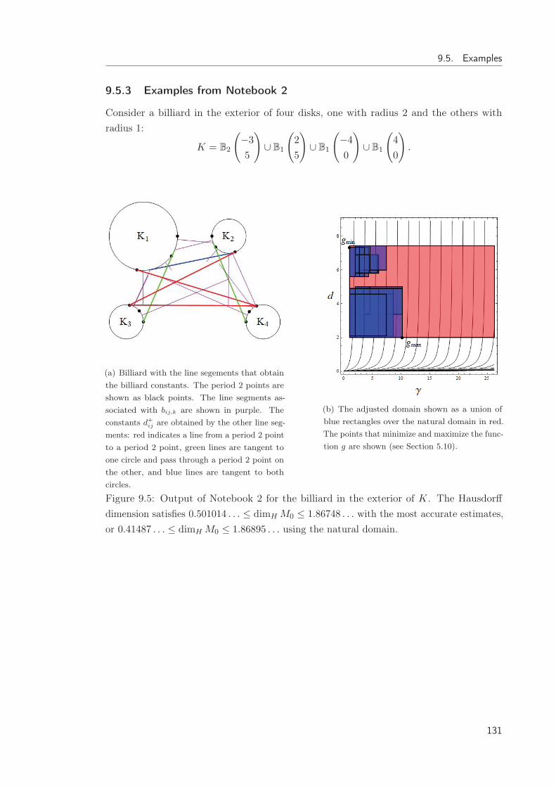
9.5. Examples

9.5.3 Examples from Notebook 2

Consider a billiard in the exterior of four disks, one with radius 2 and the others withradius 1:

K = B2

(−3

5

)∪ B1

(2

5

)∪ B1

(−4

0

)∪ B1

(4

0

).

(a) Billiard with the line segements that obtainthe billiard constants. The period 2 points areshown as black points. The line segments as-sociated with bij,k are shown in purple. Theconstants d+ij are obtained by the other line seg-ments: red indicates a line from a period 2 pointto a period 2 point, green lines are tangent toone circle and pass through a period 2 point onthe other, and blue lines are tangent to bothcircles.

(b) The adjusted domain shown as a union ofblue rectangles over the natural domain in red.The points that minimize and maximize the func-tion g are shown (see Section 5.10).

Figure 9.5: Output of Notebook 2 for the billiard in the exterior of K. The Hausdorffdimension satisfies 0.501014 . . . ≤ dimH M0 ≤ 1.86748 . . . with the most accurate estimates,or 0.41487 . . . ≤ dimH M0 ≤ 1.86895 . . . using the natural domain.

131

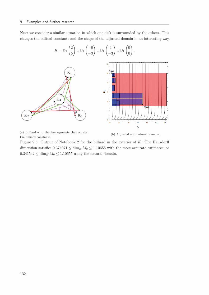
9. Examples and further research

Next we consider a similar situation in which one disk is surrounded by the others. Thischanges the billiard constants and the shape of the adjusted domain in an interesting way.

K = B1

(2

5

)∪ B1

(−6

−3

)∪ B1

(4

−3

)∪ B1

(0

0

).

(a) Billiard with the line segments that obtainthe billiard constants.

(b) Adjusted and natural domains.

Figure 9.6: Output of Notebook 2 for the billiard in the exterior of K. The Hausdorffdimension satisfies 0.374071 ≤ dimH M0 ≤ 1.10655 with the most accurate estimates, or0.341542 ≤ dimH M0 ≤ 1.10655 using the natural domain.

132

9.5. Examples

9.5.4 Examples from Notebook 3

Consider a three dimensional billiard deformation in the exterior of four unit spheresarranged in a tetrahedron, expanding linearly with α. We have

K(α) = B1

⎛⎜⎝ α

2√2

⎛⎜⎝1

1

1

⎞⎟⎠⎞⎟⎠∪B1

⎛⎜⎝ α

2√2

⎛⎜⎝

1

−1

−1

⎞⎟⎠⎞⎟⎠∪B1

⎛⎜⎝ α

2√2

⎛⎜⎝−1

1

−1

⎞⎟⎠⎞⎟⎠∪B1

⎛⎜⎝ α

2√2

⎛⎜⎝−1

−1

1

⎞⎟⎠⎞⎟⎠ .

Next we consider a similar situation in which one disk is surrounded by the others. Thischanges the billiard constants and the shape of the adjusted domain in an interesting way.

K = B1

(2

5

)∪ B1

(−6

−3

)∪ B1

(4

−3

)∪ B1

(0

0

).

(a) The deformation at α = 5. (b) Billiard constants.

(c) Hausdorff dimension.

Figure 9.7: Output of Notebook 3 for a billiard deformation in the exterior of K(α).

133

9. Examples and further research

Consider a three dimensional billiard deformation in the exterior of three unit spheresarranged in a fixed right triangle in the plane, with a fourth unit sphere rising out of theplane. Specifically, let

K(α) = B1

⎛⎜⎝0

0

0

⎞⎟⎠ ∪ B1

⎛⎜⎝12

0

0

⎞⎟⎠ ∪ B1

⎛⎜⎝0

8

0

⎞⎟⎠ ∪ B1

⎛⎜⎝3

3

α

⎞⎟⎠ .

This billiard satisfies (H) for all α ∈ R.

(a) The deformation at α = 5. (b) Billiard constants.

(c) Hausdorff dimension.

Figure 9.8: Output of Notebook 3 for a billiard deformation in the exterior of K(α).

134

9.5. Examples

9.5.5 Examples from Notebook 4

Consider the billiard deformation defined by

K(α) = B1

(−2

0

)∪ B1

(2

0

)∪ B1

(0

α

).

This is well defined for all α ∈ [∞,−2) ∪ (2,∞].

(a) The deformation at α = 5. (b) Billiard constants.

(c) Hausdorff dimension. (d) Derivative of Hausdorff dimension.

Figure 9.9: Output of Notebook 4 for the isosceles deformation. The graphs are blankedout for those values of α such that K(α) does not satisfy (H).

135

9. Examples and further research

Consider the billiard deformation defined by

K(α) = B1

(−5

0

)∪ B1

(5

0

)∪ B1

(0

10

)∪ B1

(α

4

).

(a) The deformation at α = −7. (b) Billiard constants.

(c) Hausdorff dimension. (d) Derivative of Hausdorff dimension.

Figure 9.10: Output of Notebook 4 for a billiard deformation consisting of three stationarydisks and a fourth disk moving horizontally between them. The graphs are blanked out forthose values of α such that K(α) does not satisfy (H).

136

Appendix A

Inverse of a cyclic tridiagonalmatrix

Here we prove Proposition 6.4.1 using the Sherman-Morrison formula [Bar51] to expressthe cyclic tridiagonal matrix A in terms of a tridiagonal matrix T . In fact we prove theproposition for any cyclic tridiagonal matrix. The proposition is not necessary in Chapter6 thanks to Varah’s theorem, however it is an interesting result in itself.

Proposition A.1. Let A be an invertible n × n cyclic tridiagonal matrix. If n is even,then the entries of the inverse of A alternate sign — i.e.

A−1ij = (−1)i+j |A−1

ij |.

To prove this, we use the Sherman-Morrison formula to remove the corner elements, andthen use Usmani’s formula to calculate the entries explicitly.

Theorem A.2. (Sherman-Morrison formula) [Bar51] Suppose T is an invertible squarematrix and u, v are vectors, such that 1 + v�T−1u �= 0. Then the Sherman-Morrisonformula is

(T + uv�)−1 = A−1 − T−1uv�T−1

1 + v�T−1u

Notice that A can be written as A = T + a1uu� where T is an invertible tridiagonal

matrix and u = (1, 0, . . . , 0, 1)�. Let

λ = u�T−1u = T−111 + T−1

1n + T−1n1 + T−1

nn ,

Bij = (T−1uu�T−1)ij = T−1i1 T−1

1j + T−1in T−1

1j + T−1i1 T−1

nj + T−1in T−1

nj .

Proposition A.3. Let T be an invertible tridiagonal matrix. For any i, j = 1, . . . , n wehave (−1)i+jTij > 0.

Proof. Usmani [Usm94] gives a formula for the explicit inverse of a tridiagonal matrix T .With the added assumption that the matrix is symmetric, the formula is

137

A. Inverse of a cyclic tridiagonal matrix

T−1ij =

⎧⎨⎩(−1)i+jai+1 . . . ajθi−1φj+1/θn : if i ≤ j,

(−1)i+jaj+1 . . . aiθj−1φi+1/θn : if i > j,

where θi and φi are defined by the following reccurence relation:

θ0 = 1,θ1 = T11, θi = Tiiθi−1 − a2i θi−2,

φn+1 = 1,φn = Tnn, φi = Tiiφi+1 − a2i+1φi+2.

First, θ1 = a2 + k1 > a2θ0. If θj−1 > ajθj−2 for some j, then

θj = (aj + aj+1 + kj)θj−1 − a2jθj−2 > aj+1θj−1.

So by induction,θi > ai+1θi−1 > 0 for i = 0, . . . n.

A very similar argument shows that

φi > aiφi+1 > 0 for i = 1, . . . n+ 1.

Since the terms a2, . . . , an are also positive, T−1ij = (−1)i+j |T−1

ij | as required.

Assume n is even, and define a matrix S by Sij = (−1)i+jθnT−1ij . Then Sij is always

positive and

Sij =

⎧⎨⎩ai+1 . . . ajθi−1φj+1 : if i ≤ j,

aj+1 . . . aiθj−1φi+1 : if i > j.

We have λ = u�T−1u = 1θn(S11 + Snn − 2S1n) and

Bij =(T−1uu�T−1

)ij=

(−1)i+j

θ2n(Snj − S1j)(Sni − S1i).

Proposition A.4. The matrix S satisfies the following inequalities.

1. S11Sij > S1jS1i.

2. SnnSij > SniSnj.

3. SniS1j > Sn1Sij.

4. S1iSnj > S1nSij.

Proof. Without loss of generality, assume i ≤ j. We start with the inequalities θj−1 >

ai+1 . . . ajθi−1 and φi+1 > ai+1 . . . ajφj+1.

φ2 · θi−1 > (a12 . . . aii−1)φi+1 · (a12 . . . aii−1)θ0

φ2 · (aii+1 . . . ajj−1)θi−1φj+1 > (a12 . . . aii−1)θ0φi+1 · (a12 . . . ajj−1)θ0φj+1

S11Sij > S1jS1i

as required. The rest of the inequalities are analogous.

138

Using these inequalities, and remembering that n is even, we have

S11Sij + SnnSij + SnjS1i + S1jSni > SniSnj + S1jS1i + 2Sn1Sij

(S11 + Snn − 2Sn1)Sij > S1jS1i + SniSnj − SnjS1i − S1jSni

θnλSij > (Sni − S1i)(Snj − S1j).

Now we are in position to prove Proposition A.1

Proof. Using the Sherman Morrison formula, we get

A−1ij = T−1

ij − a11 + a1λ

Bij

(−1)i+jA−1ij =

1

θnSij −

a11 + a1λ

1

θ2n(Sni − S1i)(Snj − S1j)

=θn(1 + a1λ)Sij − a1(Sni − S1i)(Snj − S1j)

θ2n(1 + a1λ)

=θnSij + a1 (θnλSij − (Sni − S1i)(Snj − S1j))

θ2n(1 + a1λ)

>Sij

θn(1 + a1λ)> 0.

139

Bibliography

[AM78] R. Abraham, J. E. Marsden: Foundations of Mechanics. Benjamin Cummings,Reading, MA (1978).

[Arb00] L. Arbogast: Du calcul des dérivations. LeVrault Frères, Strasbourg (1800).

[Arz95] C. Arzelà: Sulle funzioni di linee. Mem. Accad. Sci. Bologna, 5(5), (1895),55–74.

[Bar51] M. S. Bartlett: An inverse matrix adjustment arising in discriminant analysis.Ann. Math. Stat., 22(1), (1951), 107–111.

[Bar96] L. M. Barreira: A non-additive thermodynamic formalism and applications todimension theory of hyperbolic dynamical systems. Ergod. Theory and Dyn.Syst., 16(5), (1996), 871–927.

[BCH10] J. Ban, Y. Cao, H. Hu: The dimensions of a non-conformal repeller and anaverage conformal repeller. Tran. Amer. Math. Soc., 362(2), (2010), 727–751.

[BG11] L. Barreira, K. Gelfert: Dimension estimates in smooth dynamics: a survey ofrecent results. Ergod. Theory and Dyn. Syst., 31(3), (2011), 641–671.

[Bow72] R. Bowen: Periodic orbits for hyperbolic flows. Amer. J. Math., 94(1), (1972),1–30.

[Bow75] R. Bowen: Equilibrium States and the Ergodic Theory of Anosov Diffeomor-phisms, vol. 470 of Lect. Notes in Math. Springer, Berlin (1975).

[Bow79] R. Bowen: Hausdorff dimension of quasi-circles. Pub. Math. de l’IHÉS, 50(1),(1979), 11–25.

[BP01] L. Barreira, Ya. B. Pesin: Lectures on Lyapunov exponents and smoothergodic theory. In Smooth Ergod. Theory and Appl., vol. 69. Amer. Math. Soc.,Providence (2001), 3–90.

[CFH08] Y. Cao, D. Feng, W. Huang: The thermodynamic formalism for sub-additivepotentials. Discr. and Cont. Dyn. Sys., 20(3), (2008), 639–657.

141

Bibliography

[Che91] N. Chernov: Topological entropy and periodic points of two-dimensional hy-perbolic billiards. Func. Anal. Appl., 25(1), (1991), 39–45.

[CM06] N. Chernov, R. Markarian: Chaotic Billiards, vol. 127 of Mathematical Surveysand Monographs. Amer. Math. Soc., Providence, RI (2006).

[CP10] J. Chen, Ya. B. Pesin: Dimension of non-conformal repellers: a survey. Non-linearity, 23(4), (2010), R93.

[Det12] C. P. Dettmann: New horizons in multidimensional diffusion: the Lorentz gasand the Riemann hypothesis. J. Stat. Phys., 146(1), (2012), 181–204.

[Edg07] G. Edgar: Measure, Topology, and Fractal Geometry. Springer, New York(2007).

[Fal88] K. J. Falconer: A subadditive thermodynamic formalism for mixing repellers.J. Phys. A: Math. and General, 21(14), (1988), L737–L742.

[Fal90] K. Falconer: Fractal Geometry. Wiley, New York (1990).

[GR89] P. Gaspard, S. A. Rice: Scattering from a classically chaotic repellor. J. Chem.Phys., 90(4), (1989), 2225–2241.

[Had98] J. Hadamard: Les surfaces à courbures opposées et leurs lignes géodésique. J.Math. Pures et Appl., 4, (1898), 27–73.

[Has94] B. Hasselblatt: Regularity of the Anosov splitting and of horospheric foliations.Ergod. Theory and Dyn. Syst., 14(4), (1994), 645–666.

[Has97] B. Hasselblatt: Regularity of the Anosov splitting II. Ergod. Theory and Dyn.Syst., 17(1), (1997), 169–172.

[HJ85] R. A. Horn, C. R. Johnson: Matrix Analysis. Cambridge Univ. Press (1985).

[HS04] B. Hasselblatt, J. Schmeling: Dimension product structure of hyperbolic sets.Electron. Res. Announc. Amer. Math. Soc., 10, (2004), 88–96.

[Ika88] M. Ikawa: Decay of solutions of the wave equation in the exterior of severalconvex bodies. Ann. Inst. Fourier, 38(2), (1988), 113–146.

[Ken04] R. Kenny: Estimates of Hausdorff dimension for the non-wandering set of anopen planar billiard. Can. J. Math., 56(1), (2004), 115–133.

[KH97] A. Katok, B. Hasselblatt: Introduction to the Modern Theory of DynamicalSystems, vol. 54. Cambridge Univ. Press (1997).

[Kin73] J. Kingman: Subadditive ergodic theory. Ann. Probability, 1(6), (1973), 883–909.

142

Bibliography

[KK83] L. Kaup, B. Kaup: Holomorphic functions of several variables: an introductionto the fundamental theory, vol. 3. Walter de Gruyter (1983).

[KKPW89] A. Katok, G. Knieper, M. Pollicott, H. Weiss: Differentiability and analyticityof topological entropy for Anosov and geodesic flows. Inventiones Math., 98(3),(1989), 581–597.

[Kol58] A. N. Kolmogorov: A new metric invariant of transitive dynamical systemsand Lebesgue space automorphisms. In Dokl. Acad. Sci. USSR, vol. 119 (1958),861–864.

[Kry79] N. S. Krylov: Works on the Foundations of Statistical Physics. Princeton Univ.Press (1979).

[LM96] A. Lopes, R. Markarian: Open billiards: invariant and conditionally invariantprobabilities on Cantor sets. SIAM J. Appl. Math., 56(2), (1996), 651–680.

[Lor05] H. A. Lorentz: The motion of electrons in metallic bodies. In KoninklijkeNederlandse Akademie van Wetenschappen, Proc. Series B Phys. Sci., vol. 7(1905), 438–453.

[Lor63] E. N. Lorenz: Deterministic nonperiodic flow. J. Atmospheric Sci., 20(2),(1963), 130–141.

[Mañ90] R. Mañé: The Hausdorff dimension of horseshoes of diffeomorphisms of surfaces.Bol. Soc. Bras. Mat., 20(2), (1990), 1–24.

[MH38] M. Morse, G. A. Hedlund: Symbolic dynamics. Amer. J. Math., 60, (1938),815–866.

[Mis00] R. L. Mishkov: Generalization of the formula of Faa di Bruno for a compositefunction with a vector argument. Int. J. Math. and Math. Sci., 24(7), (2000),481–491.

[MM83] H. McCluskey, A. Manning: Hausdorff dimension for horseshoes. Ergod. Theoryand Dyn. Syst., 3(2), (1983), 251–260.

[Mor91] T. Morita: The symbolic representation of billiards without boundary condition.Tran. Amer. Math. Soc., 325(2), (1991), 819–828.

[Ose68] V. I. Oseledets: A multiplicative ergodic theorem. Lyapunov characteristicnumbers for dynamical systems. Tran. Moscow Math. Soc., 19, (1968), 197–221.

[Osk06] W. H. Oskay: Christmas Chaos. http://www.evilmadscientist.com/2006/christmas-chaos/ (2006). Accessed 10 July 2014.

[Pes88] Ya. B. Pesin: Dimension type characteristics for invariant sets of dynamicalsystems. Russian Math. Surv., 43(4), (1988), 111–151.

143

Bibliography

[Pes97] Ya. B. Pesin: Dimension Theory in Dynamical Systems: Contemporary Viewsand Applications. Chicago Lect. Math. Uni. of Chicago Press (1997).

[PP84] Ya. B. Pesin, B. Pitskel’: Topological pressure and the variational principle fornoncompact sets. Func. Anal. and Appl., 18(4), (1984), 307–318.

[PP90] W. Parry, M. Pollicott: Zeta Functions and the Periodic Orbit Structure ofHyperbolic Dynamics, vol. 187–188 of Astérisque. Soc. Math. France, Montrouge(1990).

[PS92] V. Petkov, L. Stoyanov: Geometry of Reflecting Rays and Inverse SpectralProblems. Wiley, Chichester (1992).

[Rud64] W. Rudin: Principles of Mathematical Analysis. McGraw-Hill, New York, 3rdedn. (1964).

[Rue73] D. Ruelle: Statistical mechanics on a compact set with Zv action satisfyingexpansiveness and specification. Tran. Amer. Math. Soc., 185, (1973), 237–251.

[Rue97] D. Ruelle: Differentiation of SRB states. Comm. Math. Phys., 187(1), (1997),227–241.

[Saw01] J. Sawada: Generating bracelets in constant amortized time. SIAM J. Com-puting, 31(1), (2001), 259–268.

[Sin70] Ya. G. Sinai: Dynamical systems with elastic reflections. Russian Math. Surv.,25(2), (1970), 137–191.

[Sin79] Ya. G. Sinai: Development of Krylov’s ideas (1979). Afterword to N. S. Krylov’sWorks on the Foundations of Statistical Physics [Kry79].

[Sjö90] J. Sjöstrand: Geometric bounds on the density of resonances for semiclassicalproblems. Duke Math. J., 60(1), (1990), 1–57.

[SL02] S. Sridhar, W. Lu: Sinai billiards, Ruelle zeta-functions and Ruelle resonances:microwave experiments. J. Stat. Phys., 108(5-6), (2002), 755–765.

[Sma67] S. Smale: Differentiable dynamical systems. Bull. Amer. Math. Soc., 73(6),(1967), 747–817.

[SOY99] D. Sweet, E. Ott, J. A. Yorke: Topology in chaotic scattering. Nature,399(6734), (1999), 315–316.

[SSS92] J. Schmeling, R. Siegmund-Schultze: Hölder continuity of the holonomy mapsfor hyperbolic basic sets I. Ergod. Theory and Related Topics III, 1514, (1992),174–191.

144

Bibliography

[Sto89] L. Stoyanov: An estimate from above of the number of periodic orbits forsemi-dispersed billiards. Comm. Math. Phys., 124(2), (1989), 217–227.

[Sto99] L. Stoyanov: Exponential instability for a class of dispersing billiards. Ergod.Theory and Dyn. Syst., 19(1), (1999), 201–226.

[Sto01] L. Stoyanov: Spectrum of the Ruelle operator and exponential decay of corre-lations for open billiard flows. Amer. J. Math., 123(4), (2001), 715–759.

[Sto11] L. Stoyanov: Non-integrability of open billiard flows and Dolgopyat-typeestimates. Ergod. Theory and Dyn. Syst., 32(1), (2011), 295–313.

[Tho79] J. A. Thorpe: Elementary Topics in Differential Geometry. Springer, NewYork (1979).

[Tri82] C. Tricot: Two definitions of fractional dimension. Math. Proc. CambridgePhil. Soc., 91(1), (1982), 57–74.

[Usm94] R. A. Usmani: Inversion of a tridiagonal Jacobi matrix. Linear Alg. and ItsAppl., 212, (1994), 413–414.

[Var75] J. M. Varah: A lower bound for the smallest singular value of a matrix. LinearAlg. and Its Appl., 11(1), (1975), 3–5.

[Wal75] P. Walters: A variational principle for the pressure of continuous transforma-tions. Amer. J. Math., 97(4), (1975), 937–971.

[Wal82] P. Walters: An Introduction to Ergodic Theory, vol. 79. Springer, New York(1982).

[Wri13] P. Wright: Estimates of Hausdorff dimension for non-wandering sets of higherdimensional open billiards. Can. J. Math., 65, (2013), 1384–1400.

[Wri14a] P. Wright: Differentiability of Hausdorff dimension of the non-wandering set ina planar open billiard (2014). ArXiv:1401.1002v2.

[Wri14b] P. Wright: Hausdorff dimension of non-wandering sets for average conformalhyperbolic maps (2014). ArXiv:1401.1005v2.

[ZCB09] Y. Zhao, Y. Cao, J. Ban: The Hausdorff dimension of average conformalrepellers under random perturbation. Nonlinearity, 22(10), (2009), 2405–2416.

145