Dimas Mateus Fazio, Thiago Christiano Silva, Benjamin ... · Inflation Targeting and Financial...

Inflation Targeting and Financial Stability:does the quality of institutions matter?

Dimas Mateus Fazio, Thiago Christiano Silva, Benjamin Miranda Tabak and Daniel Oliveira Cajueiro

January 2018

470

ISSN 1518-3548 CGC 00.038.166/0001-05

Working Paper Series Brasília no. 470 January 2018 p. 1-37

Working Paper Series

Edited by the Research Department (Depep) – E-mail: [email protected]

Editor: Francisco Marcos Rodrigues Figueiredo – E-mail: [email protected]

Co-editor: José Valentim Machado Vicente – E-mail: [email protected]

Editorial Assistant: Jane Sofia Moita – E-mail: [email protected]

Head of the Research Department: André Minella – E-mail: [email protected]

The Banco Central do Brasil Working Papers are all evaluated in double-blind refereeing process.

Reproduction is permitted only if source is stated as follows: Working Paper no. 470.

Authorized by Carlos Viana de Carvalho, Deputy Governor for Economic Policy.

General Control of Publications

Banco Central do Brasil

Comun/Divip

SBS – Quadra 3 – Bloco B – Edifício-Sede – 2º subsolo

Caixa Postal 8.670

70074-900 Brasília – DF – Brazil

Phones: +55 (61) 3414-3710 and 3414-3565

Fax: +55 (61) 3414-1898

E-mail: [email protected]

The views expressed in this work are those of the authors and do not necessarily reflect those of the Banco Central do

Brasil or its members.

Although the working papers often represent preliminary work, citation of source is required when used or reproduced.

As opiniões expressas neste trabalho são exclusivamente do(s) autor(es) e não refletem, necessariamente, a visão do Banco Central do Brasil.

Ainda que este artigo represente trabalho preliminar, é requerida a citação da fonte, mesmo quando reproduzido parcialmente.

Citizen Service Division

Banco Central do Brasil

Deati/Diate

SBS – Quadra 3 – Bloco B – Edifício-Sede – 2º subsolo

70074-900 Brasília – DF – Brazil

Toll Free: 0800 9792345

Fax: +55 (61) 3414-2553

Internet: http//www.bcb.gov.br/?CONTACTUS

Non-Technical Summary

Inflation targeting has been blamed by several international specialists and authorities as

one of the causes of the recent 2007-2008 financial crisis. On the one hand, governments

may have focused too much in maintaining low inflation and may not have perceived the

building of financial imbalances that led to the crisis. In this way, they may have been

victims of their own success, also known as the “paradox of credibility.” On the other

hand, there is an alternative theory that states that price stability is a sufficient condition

to financial stability. According to this traditional view, when the inflation rate is close to

the inflation target, then agents’ expectations are anchored, which increases the

investment returns’ forecast ability. Despite the existence of these two opposing views,

there is not much empirical evidence on which one holds for the real world.

Our paper links these two otherwise conflicting views regarding inflation targeting and

financial stability by also bringing into the analysis how the national population of

countries perceive the quality of their government institutions. To support our empirical

findings, we use a comprehensive bank-level data from 66 countries and ask: (a) whether

banks from inflation targeting countries benefit from this policy in terms of higher and

less volatile profits; and (b) if this result depends on the level of institutional quality of

countries. We proxy the quality of government institutions as perceived by the national

population using the Transparency International’s corruption perception index. We find

that inflation targeting relates positively to the financial stability of a country’s banking

system. We also show an inverse U-shaped relationship between institutional quality and

financial stability, which provides empirical evidence on the validity of both theories that

link inflation targeting and financial stability.

3

Sumário Não Técnico

O regime de metas de inflação tem sido culpado por vários especialistas e autoridades

internacionais como uma das causas da recente crise financeira de 2007-2008. Por um

lado, ao focar somente no controle da inflação, os governos podem não ter percebido o

surgimento e desenvolvimento de desequilíbrios financeiros que aumentaram a

fragilidade financeira dos países e culminaram na crise. Os governos, portanto, podem ter

sido ser vítimas de seu próprio sucesso, fenômeno que é conhecido como o “paradoxo da

credibilidade”. Por outro lado, a visão macroeconômica tradicional defende que a

estabilidade de preços é condição suficiente para a estabilidade financeira. De acordo com

esta visão, uma inflação dentro da meta ancora as expectativas dos agentes, aumentando

a previsibilidade do retorno de investimentos e diminuindo incertezas financeiras. Apesar

dessas visões opostas, não há evidências claras sobre qual delas se aplica ao mundo real.

Nesse trabalho, tentamos ligar essas duas teóricas que, em princípio, seriam conflitantes

usando um índice de qualidade das instituições governamentais, o qual é mensurado a

partir da percepção da população nacional dos países. Este artigo utiliza dados bancários

de 66 países e pergunta: (a) se bancos de países que adotam metas de inflação se

beneficiam com maior lucro e menor volatilidade de seus retornos; e (b) se este resultado

depende da qualidade das instituições governamentais dos países. Como proxy para

qualidade das instituições governamentais, utilizamos o índice de percepção de corrupção

calculado pela Transparency International. Encontramos que a implementação de metas

de inflação está positivamente relacionada à estabilidade bancária daqueles países.

Verifica-se também a existência de um relacionamento em formato de U invertido entre

qualidade das instituições e estabilidade financeira, o que provê um subsídio empírico

para a validez das duas teorias que unem estabilidade financeira e regime de metas de

inflação.

4

Inflation Targeting and Financial Stability:does the quality of institutions matter?

Dimas Mateus Fazio*

Thiago Christiano Silva **

Benjamin Miranda Tabak***

Daniel Oliveira Cajueiro****

Abstract

Inflation targeting (IT) has recently been seen as one of the main causes of the au-thorities’ unresponsiveness to the build up of financial imbalances during the recentfinancial crisis. We take data from banks from 66 countries for the period of 1998-2014 and compare how institutional quality as perceived by the national populationimpacts financial stability in countries that adopted IT with those that did not. Wefind that, while banks from IT countries with high quality of institutions do not havetheir stability significantly enhanced by this policy (the “paradox of credibility”),countries with average levels of quality of institutions seem to benefit from it. Inaddition, in the estimations, IT and financial stability are negatively associated incountries with low levels of institutional quality, which is consistent with the factthat governments must have at least some trust of their population in order to con-duct effective economic policies. This inverted U-shaped relationship between ITand financial stability as function of the institutional quality reflects the two oppos-ing views in the literature regarding this topic.

Keywords: quality of institutions, inflation targeting, financial stability, transparency.JEL Classification: D40, G21, G28.

The Working Papers should not be reported as representing the views of the BancoCentral do Brasil. The views expressed in the papers are those of the authors and donot necessarily reflect those of the Banco Central do Brasil

*London Business School, e-mail: [email protected]**Research Department, Banco Central do Brasil, e-mail: [email protected]

***Universidade Catolica de Brasılia, e-mail: [email protected]****Universidade de Brasılia, e-mail: [email protected]

5

1 Introduction

The quality of institutions gains significant importance during financial crisis (Klompand de Haan, 2014). Countries with high quality of institutions should be able to formu-late policies to deal more effectively with adverse shocks than countries that suffer fromlow institutional quality. Recent discussion triggered by the financial crisis has pointed in-flation targeting (IT) as one important reason for the failure of the government authoritiesto respond to developing financial imbalances and rising financial instability for severalreasons. First, by focusing in achieving the inflation target, governments may have over-looked the situation in the financial market (Blanchard et al., 2010). Second, low andstable inflation coupled with a credible anti-inflationary policy can make it harder for fi-nancial imbalances, such as asset bubbles, to show up in inflation indexes. In fact, Amatoand Shin (2003) argue that in a model in which agents have imperfect information on thestate of the economy (such as inflation), but in which they fully believe in a public signalissued by the government (i.e. high credible signal), agents beliefs might be distorted,since they might put more weight into this public signal than in actual fundamentals. Inthis case, inflation levels would lose its informativeness about economic (demand andcost) conditions and thus financial imbalances might develop. Therefore, governmentscan be a victim of their own success, phenomenon of which the literature terms as the“paradox of credibility” (Borio, 2005, 2006; Borio and Lowe, 2002; Montes and Peixoto,2014). Third, a commitment to low inflation levels makes the economic policy too looseduring normal times. Thus, the policy rate approaches the zero lower-bound, reducingthe margin for any adjustment on the interest policy rates should any economic down-turn arise. We contribute to the literature by evaluating the relationship between IT andfinancial instability while controlling for quality of institutions.

Notwithstanding this criticism, a traditional view (the Schwartz (1995) hypothesis)argues that periods of unstable price levels can lead to incorrect inferences about the fu-ture real returns of investments. This may result in flawed lending/borrowing decisions,increasing loan defaults, compromising the banking system’s loan portfolio, and increas-ing bankruptcies. Inflation targeting improves the predictability of economic policy andreduces the degree of uncertainty about the price level over the long run (the price stabilitychannel). Bordo and Wheelock (1998) argue that among the several financial crises thatoccurred during the XIX and XX centuries, the most severe financially distressing eventsoccurred after unexpected and substantial disinflation.

Empirical papers that test how the quality of government institutions and inflationtargeting in different countries impact financial stability are surprisingly rare.1 Using

1Among the papers that are close to our approach, we highlight Fouejieu (2017), Kim and Mehrotra(2017), and Hove et al. (2017). However, they do not explore the non-linearity between the quality ofinstitutions and the adoption of an IT regime as we propose in this paper.

6

bank-level data from 66 countries over the period of 1998–2014, and measures of qualityof government institutions as perceived by the national population, our paper provides em-pirical evidence that attempts to bridge this gap in the literature. We employ two measuresof quality of institutions: the Corruption Perception Index of the Transparency Interna-tional, and the Government Effectiveness Index of World Bank’s Governance Indicators(WGI). We interact these variables with dummies that flag whether a specific countryadopted IT, as defined by the International Monetary Fund2 in a triple DiD approach.Banks in IT countries (treated) are compared with those in non-IT countries (control)for different levels of quality of institutions. Our benchmark specification controls fortime-invariant bank characteristics, and both bank- and country-level controls.

Among the advantages of our proxies to institutional quality are the fact that theyare publicly available and are calculated by international trusted institutions. This avoidssubjective data mining issues and improves the accountability of the paper. Moreover,these measures are related to the agents’ trust in government’s communication about theireconomic policies. We argue that the population of a non-corrupt country put more trustin their government than the population of a highly corrupt country. Thus, we can testwhether the IT impact on financial stability depends on the quality of national govern-ments. Intuitively, there must be a lower bound for the trust in the authorities in order forany economic policy to be effective. In addition, we can also test if there is also an upperbound, i.e. when the institutional quality is so high that the benefit to financial stabilitymight not be significant anymore as Amato and Shin (2003) highlight. Finally, we mini-mize endogeneity concerns because government authorities cannot change these measuresin the short term. In addition, since governments cannot easily manipulate agents’ per-ception on corruption nor institutional quality, we believe that our measures are safe fromthis manipulation.

We find that banks from IT countries perceived as having high quality of institu-tions are neither more nor less stable than their non-IT counterparts. Thus, trust in thegovernment policies by itself does not appear to increase financial stability of IT coun-tries, which is consistent with Borio and Lowe (2002)’s “paradox of credibility.” Second,banks from countries that have institutions perceived as being of low quality seem to un-derperform under an IT policy. It appears that for an IT policy to have positive spilloverson financial stability, a minimum level of credibility in the government is needed. Third,the price stability channel might lead to a higher financial stability of banks located incountries whose institutions are perceived as having average levels of quality. Thus, the

2According to Mishkin (2004) and Heenan et al. (2006), inflation targeting consists of four elements:(i) an explicit CB mandate to pursue price stability as the primary objective of monetary policy and ac-countability for performance in achieving the objective; (ii) explicit quantitative targets for inflation; (iii)policy actions based on a forward-looking assessment of inflation pressures that considers a wide range ofinformation; and (iv) increased transparency of monetary policy strategy and implementation.

7

commitment to price stability and the greater transparency and accountability, which arecharacteristics of an inflation targeter country, relate to lower bank risk-taking for banksin countries that do not have “too much” nor “too little” levels of quality of institutions,as perceived by their population.

A possible concern, as in several other cross-country studies, is the possible ex-istence of unobserved factors correlated with both the quality of institutions and banks’risk-taking that might also explain our results. Ideally, one could control for such reformsby the use of country-year fixed effects. Nevertheless, this is not possible since such fixedeffects would be collinear with the interaction between the IT dummy and the qualityof institutions measure. We then perform several robustness tests. First, we show thatthe introduction of country-specific controls - such as GDP per capita, inflation, amongother financial depth variables - does not change our results significantly. Second, wealso add region-year fixed effects to account for time-varying shocks that are common toneighboring countries and that may be affecting both financial stability and the qualityof the institutions. Third, in the spirit of La-Porta et al. (1997, 1998), we also add legalorigin-year fixed effects to account for different trends in countries with different legalsystems. It is widely accepted that countries with the same legal origin are subject tosimilar constraints, which may affect their economic and financial development, as wellas the functioning of their banking markets. In all these specifications, our results seemto hold satisfactorily.

Related literature: Previous evidence on the IT–financial stability relationship isscarce. The paper that is closest ours is Fazio et al. (2015). These authors find that: (i)banks from IT countries are, on average, more stable than non-IT banks; (ii) this resultholds even in periods of global illiquidity (such as during the 2007-2008 financial crisis);and (iii) systemically important banks from IT countries are also more stable than theirnon-IT counterparts. Fazio et al. (2015)’s paper, however, does not provide the necessaryattention to the role of institutional quality in shaping financial stability in IT and non-ITcountries. In fact, inflation targeters were only compared with their non-IT counterparts.This study therefore adds to this literature by differentiating IT countries with respect tolevels of quality of their government institutions.

Our paper is related to the literature on government transparency and central bankindependence. The literature has empirically shown that central bank transparency has arole in reducing the volatility of inflation (Dincer and Eichengreen, 2014) and the mon-etary base growth which also leads to a lower inflation (Bodea and Hicks, 2015). In ad-dition, Backus and Driffill (1984) use a reputation model together with a macroeconomicpolicy game to show that imperfect credibility leads to output loss, since the govern-ment would have to be tougher so as to convince the private sector of its commitment.Ruge-Murcia (1995) analyzes a rational expectations model where the government com-

8

municates an inflation target but may or may not adopt the corresponding fiscal policy.Agents form their estimates from observables – i.e. inflation, output, and public expendi-tures – as part of their money demand decision. Institutional quality can also be seem ashow positive or credible the population see the government. A policy that is conductedby a government with institutions perceived as having low quality can endogenously fail.While these papers focus on the effects of government transparency and central bank in-dependence on price stability, we take this analysis further by showing that the qualityof government institutions affects financial stability through the inflation target policy,whose success crucially depends on agents’ trust on the government.

The remainder of this paper is organized as follows. Section 2 discusses the data,sources and variables employed in our empirical specification. Section 3 presents theempirical results with the different robustness tests. Finally, Section 4 presents the overallconclusions of the paper.

2 Data and Methodology

In this section, we explain the main empirical model, the variables employed, andtheir sources. Our main goal is to estimate how the relationship between financial stabilityand the IT policy changes with a measure of quality of government institutions. To do so,we estimate the following regression:

Financial Stabilityikt = α0 +αi +αt +β1ITkt +β2Quality Inst.kt +β3Quality Inst.2kt (1)

+ β4ITkt ∗Quality Inst.kt +β5ITkt ∗Quality Inst.2kt +Z

∑z=1

γzXz,ikt + eikt ,

where Financial Stabilityikt is a financial stability proxy - explained below - for bank i

that operates in country k at period t; IT is a dummy equal to one if the country k is aninflation targeter at period t; Quality Inst. is a proxy for the quality of institutions, andXz,ikt is a vector of country- and bank-specific controls. Finally, αi and αt are bank andtime fixed effects, respectively. As explained in the next section, since we consider allbanks operating in a particular country as our group variable, then controlling for bankfixed effects embed the country-level fixed effects. Finally, according to the literature,we also employ robust standard errors clustered by country to avoid understated standarderrors when the group (banks) is more detailed than the main regressor’s level of variation(countries).3

3See Donald and Lang (2007) and Bertrand et al. (2004) for detailed information.

9

2.1 Bank-level data

We draw bank-specific balance sheet data from Bankscope, a financial databasedistributed by BVD-IBCA, and convert these data into US dollars to guarantee accountinguniformity among countries. Initially, the data included the population of unconsolidatedfinancial statements of commercial and specialised credit government banks (that act ascommercial banks) in the database (both listed and not listed). The use of unconsolidatedfinancial statements avoids double-counting financial statements, since some banks maycontrol others that are also present in Bankscope. We, therefore, have access to dataregarding state-owned, private, and even foreign subsidiaries of banks that operate withineach country covered in the database.4 Finally, mergers and acquisitions are not a problemsince from the moment where such operation is realized, the acquired bank stop to reportand the acquiring bank incorporates it.

After cleaning the data for periods with missing, negative or zero values for therelevant balance sheet data, and observations with missing country-specific data, the finalsample is an unbalanced panel including 5458 banks in 66 countries during the period1998-2014 (17 years) totaling 159,000 observations. This dataset is among the mostrepresentative in the banking literature in terms of the number of years and banks.

We employ this balance-sheet data set to construct our benchmark measure of finan-cial stability for equation (1): the Z-score. Many studies that evaluate bank risk-takingbehaviour employ the Z-score as a measure of financial soundness. The literature is vast,encompassing researches prior to the global financial crisis, such as in Boyd and Run-kle (1993); Demirguc-Kunt and Huizinga (2010); Laeven and Levine (2009); Merciecaet al. (2007), and also post crisis, such as in Fiordelisi and Mare (2014); Fu et al. (2014).Using data from 2004 to 2012 from U.S. commercial banks, Chiaramonte et al. (2016)find that the Z-score, on average, can predict 76% of bank failures, which highlights theimportance of such measure as an indicator of financial soundness.

According to Roy (1952), the Z-score measures how far a specific bank is from in-solvency, which takes place when equity is insufficient to cover losses (Equity < Losses).Mathematically, the Z-score is equal to the number of return over assets (ROA) standarddeviations a bank’s ROA must decrease to exceed its equity ratio. One alternative overusing the Z-Score is Adrian and Brunnermeier (2016)’s ∆ CoVaR method. This method-ology calculates the contribution of a particular bank to the risk of the entire system, whiletraditional risk measures focus on the risk of individual institutions. Despite these advan-tages, the ∆ CoVaR method is employable only to banks that are listed in their respectivecountries (see Adrian and Brunnermeier, 2016, who use data of Compustat/CRSP to em-ploy the ∆ CoVaR to the US). While this analysis appears to be satisfactory for developed

4For instance, Citibank will have one financial statement in the US, related to its operations in thatcountry only; and one financial statement in each country in which it has foreign subsidiaries

10

economies, it would leave out both state-owned banks and foreign subsidiaries (which arein majority unlisted) that are important for the banking system of emerging economies.For instance, we could not calculate the systemic risk contribution of the big four state-owned banks of China before their IPO (the last bank to go public was the AgriculturalBank in 2010).

As in Laeven and Levine (2009), since the Z-score is skewed, we use its naturallogarithm, which is normally distributed, as our proxy for financial stability of a bank:

ln(Z-scoreit) = ln(

ROAit +Capital Ratioit

σ(ROA)i,t:t−3

)(2)

This measure is often employed in cross-sectional OLS models in which the mean andstandard deviation of ROA for the whole period can be calculated. However, we proposeto calculate this measure for each year to maintain the Z-score as a panel variable. Wedo so by calculating the standard deviation of ROA for each bank using information fromthe last 4 years (current + previous 3 years) Therefore, rather than eliminating the timedimension of the analysis, this approach reduces the maximum number of periods from17 to 14.

To deepen our analysis, we also divide the Z-score in its components: one partrelates to the returns (Risk-Adjusted ROA - RAROA):5

RAROAit = ln(

ROAit

σ(ROA)i,t:t−3

); (3)

and the other to the volatility of these returns:

ROA Volatilityit = ln(σ(ROA)i,t:t−3); (4)

Bank balance sheet variables are also included as controls. First, we include thenatural logarithm of total assets (SIZE). Another balance-sheet variable is the liquidityratio, which is liquid assets divided by total assets. We also include the ratio of non-interest income to total income to proxy for banks’ nontraditional activities (Lozano-Vivasand Pasiouras, 2010). We add the ratio between total customer deposits and total assets

5There is a problem in applying the natural logarithm of the Z-score or the Risk-Adjusted Returns,because these variable can take negative values as well. These negative values are possible when the bank’sprofitability offsets its capital ratio (in the case of the Z-score), or when the average ROA is negative(in the Risk-Adjusted Returns case), indicating that the bank is near insolvency. To solve this problem,instead of just deleting these observations, we follow Bos and Koetter (2009) who employs an additionalindependent variable, the negative Z-score/RAR indicator (NZI/NRI). This variable takes the value 1 whenthe Z-score/RAR ≥ 0 and is equal to the absolute value of the Z-score/RAR when Z-score/RAR < 0. Wealso alter the Z-score/RAR to take the value 1 when they are negative. Since we delete observations whosedependent variable are in the lower and upper percentile in our benchmark estimations, this problem willonly occur in the Risk-Adjusted Profits specifications. The Z-score does not assume negative values fromits 1st to 99th percentile.

11

to proxy for intermediation. Finally, we consider the costs to assets ratio to control forbank’s cost performance.

2.2 Country-Level Data

This section explains the country-level variables employed in our empirical specifi-cations. First, we include countries’ economic activity as controls. This set of variablesincludes two indices created by the Heritage Foundation, i.e., property rights and finan-cial freedom6, the GDP growth, and the consumer price index (CPI) both reported in theWorld Bank’s World Development Indicators (WDI).

We also include variables related to the financial development of the country. Thisset of variables includes banking market aggregates calculated from the balance-sheetdata contained in Bankscope, i.e., (a) the density of deposits (ratio of aggregate depositsto land area) and (b) the ratios of aggregate equity to assets, domestic credit to privatesector (as % of GDP) in the WDI, and a banking market concentration measure, i.e. theHerfindahl-Hirschmann Index (HHI).

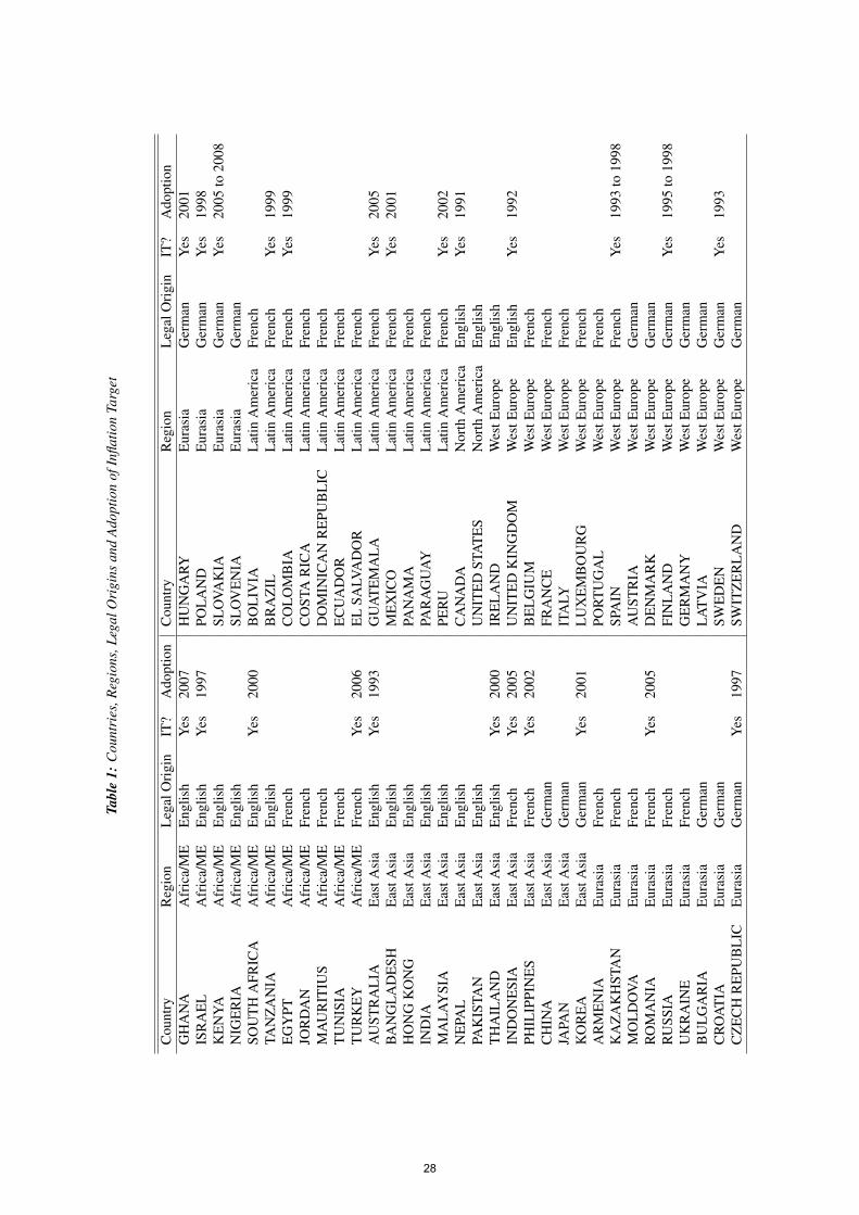
We also divide countries into 6 major geographical regions according to authors’own research: Africa and Middle East, Eurasia, Latin America, North America, South-East Asia, and Western Europe. We use this classification when we control for regionalspecific shocks by adding region-year fixed effects in our specifications. In the samefashion, we also classify the countries into 3 different legal origins: English, French andGerman/Nordic. We follow the classifications of La-Porta et al. (2008, 1997, 1998) andDjankov et al. (2003) and complement this information by checking the CIA World Fact-book and additional research.7 Table 1 lists the countries in our sample, and their respec-tive region and legal origin.

2.3 Inflation Targeting Countries

One of the main independent variable is a dummy variable equal to one if the bankoperates in an inflation targeting country k during year t (ITkt). Currently, 26 countrieshave adopted inflation targets. In addition, 3 other countries have previously adopted thispolicy but abandoned it after joining the Euro. Table 1 lists these countries as well as

6According to La-Porta et al. (1998), stronger creditor protection leads to the better development of thefinancial market and more favorable financial contracts. On the other hand, strong creditor protection maylead to excessive lending to risky enterprises, increasing the likelihood of financial crises (Houston et al.,2010). Regarding financial liberalization, several papers have shown that it impacts risk, such as Fang et al.(2014) who support the view that liberalizing reforms have had a great positive impact on bank stability oftransition economies.

7Ex-socialist countries are considered transition economies that are returning to their original legalsystem, as La-Porta et al. (2008) argument. Therefore, we list these transitional economics according totheir original legal origin instead of assigning them to a socialist legal system.

12

the years in which IT took place. These data were drawn from the IMF website, Roger(2010) and the authors’ own research. Note first that after cleaning the bank level data,we remain with 24 countries that adopted IT at any point in time.

2.4 Measures of Quality of Government Institutions

This paper uses the following two measures of quality of institutions available forall the 66 countries in the database:

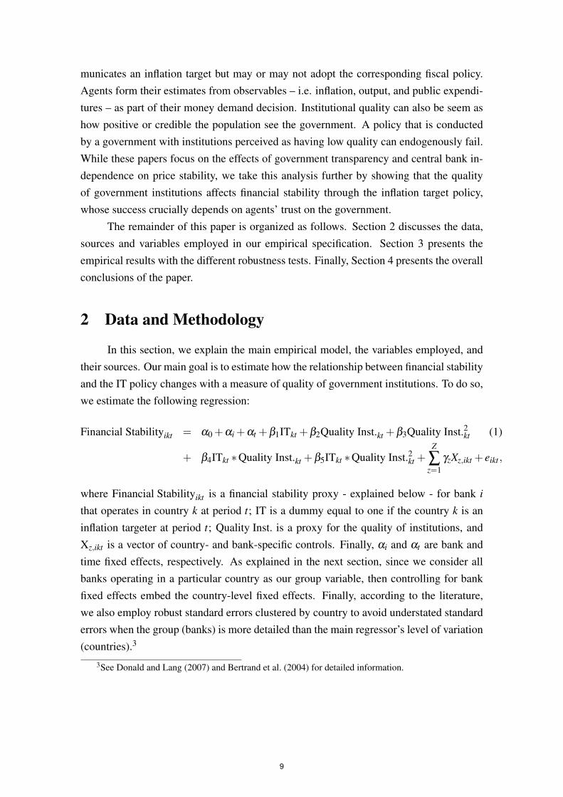
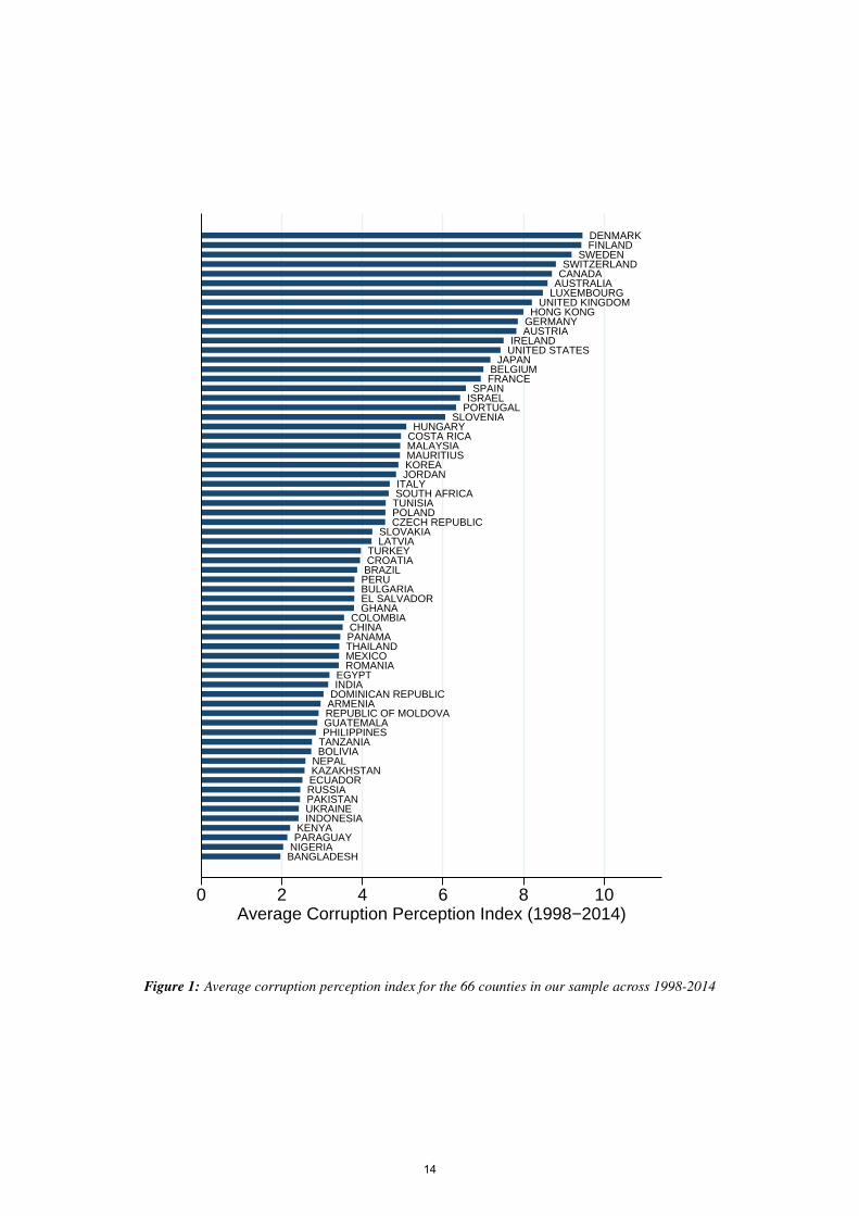
(i) the Corruption Perception Index of the Transparency International, that tests theperception of public sector corruption in several countries. The higher is this, themore a country’s citizens perceive their government as transparent and accountable,i.e., the less corrupt they are in the eyes of their population. This index varies from0 (more corruption) to 10 (less corruption).

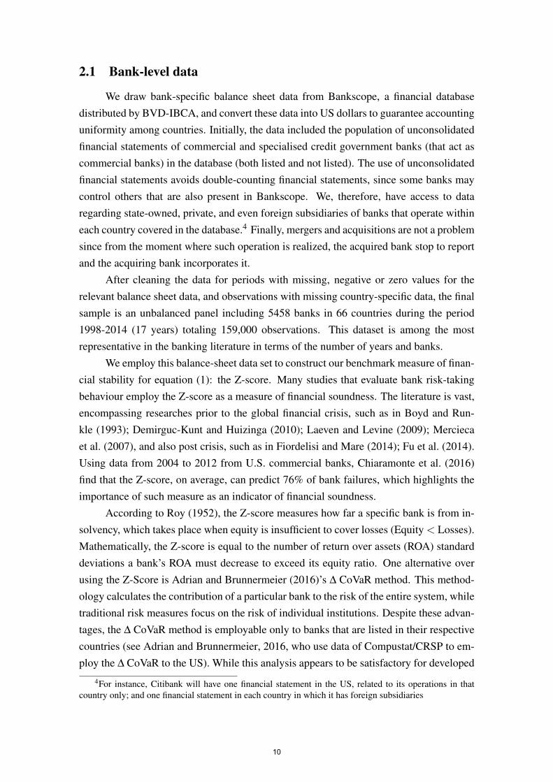
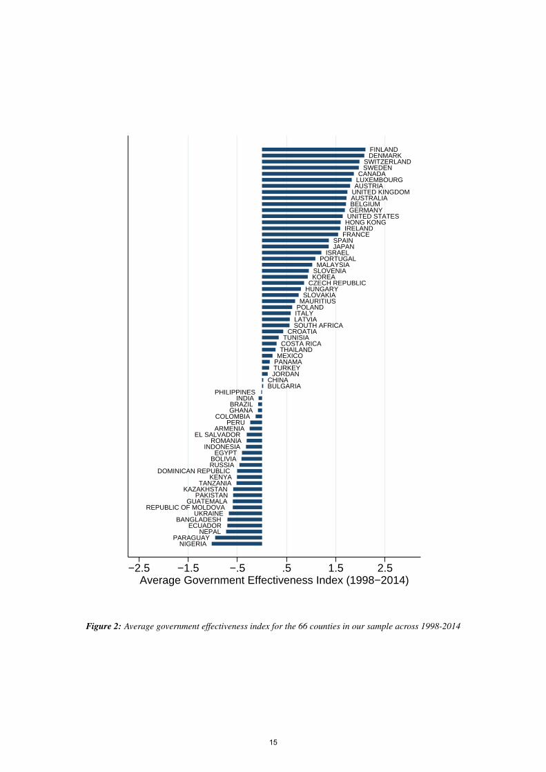
(ii) the Government Effectiveness Index of the WGI from the World Bank. This mea-sure captures perceptions of the quality of public services, of civil services, and ofpolicy formulation and implementation, as well as the extent of the government’scommitment to these policies. This index is measured in units of a standard normaldistribution, with mean zero and standard deviation of one, running from -2.5 to2.5. Higher values corresponds to better government effectiveness.

Figures 1 and 2 display the average levels of the corruption perception and thegovernment effectiveness indices of the countries in our sample across 1998–2014, re-spectively. We observe a significant heterogeneity across countries and a high correlationbetween both indices. Scandinavian countries that are present in our sample normallyshow high levels of the corruption perception index, meaning country’s citizens perceivetheir government as highly transparent and accountable. In contrast, countries with lowcorruption perception indices are not regionally localized and therefore vary worldwide,with representative countries in Africa (Kenya, Nigeria), Europe (Ukraine), South Amer-ica (Paraguay) and Asia (Bangladesh, Indonesia).

Both of these measures fit our analysis because they reflect the people’s skepticismregarding the policies of their own government. As previously discussed, an IT policywill only be successful if agents believe the communication of government authoritiesand their commitment in following their economic policies. Only this way would infla-tion expectations be consistent with the economic policy objectives and financial stabilitywould be achieved (Svensson, 2010). On the other hand, Borio and Lowe (2002) arguethat too much credibility might actually lead to an undesirable effect in which agents’expectations become decoupled from actual fundamentals (Amato and Shin, 2003), andfinancial imbalances are harder to identify. As a result, inter-sector price distortions might

13

BANGLADESHNIGERIAPARAGUAYKENYA

INDONESIAUKRAINEPAKISTANRUSSIAECUADORKAZAKHSTANNEPAL

BOLIVIATANZANIAPHILIPPINESGUATEMALAREPUBLIC OF MOLDOVAARMENIADOMINICAN REPUBLICINDIAEGYPT

ROMANIAMEXICOTHAILANDPANAMACHINACOLOMBIA

GHANAEL SALVADORBULGARIAPERUBRAZILCROATIATURKEY

LATVIASLOVAKIA

CZECH REPUBLICPOLANDTUNISIASOUTH AFRICAITALY

JORDANKOREAMAURITIUSMALAYSIACOSTA RICAHUNGARY

SLOVENIAPORTUGALISRAELSPAIN

FRANCEBELGIUM

JAPANUNITED STATESIRELAND

AUSTRIAGERMANYHONG KONG

UNITED KINGDOMLUXEMBOURGAUSTRALIACANADASWITZERLAND

SWEDENFINLANDDENMARK

0 2 4 6 8 10Average Corruption Perception Index (1998−2014)

Figure 1: Average corruption perception index for the 66 counties in our sample across 1998-2014

14

NIGERIAPARAGUAY

NEPALECUADOR

BANGLADESHUKRAINE

REPUBLIC OF MOLDOVAGUATEMALA

PAKISTANKAZAKHSTAN

TANZANIAKENYA

DOMINICAN REPUBLICRUSSIABOLIVIA

EGYPTINDONESIA

ROMANIAEL SALVADOR

ARMENIAPERU

COLOMBIAGHANABRAZIL

INDIAPHILIPPINES

BULGARIACHINA

JORDANTURKEYPANAMAMEXICOTHAILANDCOSTA RICATUNISIA

CROATIASOUTH AFRICALATVIAITALYPOLANDMAURITIUSSLOVAKIAHUNGARYCZECH REPUBLIC

KOREASLOVENIAMALAYSIAPORTUGAL

ISRAELJAPANSPAIN

FRANCEIRELANDHONG KONGUNITED STATESGERMANYBELGIUMAUSTRALIAUNITED KINGDOMAUSTRIALUXEMBOURGCANADA

SWEDENSWITZERLAND

DENMARKFINLAND

−2.5 −1.5 −.5 .5 1.5 2.5Average Government Effectiveness Index (1998−2014)

Figure 2: Average government effectiveness index for the 66 counties in our sample across 1998-2014

15

emerge, such as bubbles in the household sector without agents’ and authorities realizingit.

Besides the clear implications of corruption on the trust in the institutions, one canalso argue that corruption and inflation are linked (Al-Marhubi, 2000). First of all, thereseems to be a negative correlation between tax revenue and corruption (Ghura, 1998;Imam and Jacobs, 2007; Tanzi and Davoodi, 2000). Thus, the government of a corruptcountry would have to resort to seignorage (inflation tax) as a source of revenue. Inaddition, by reducing revenues and increasing public spending, corruption leads to largefiscal deficits, with inflationary consequences. Therefore, an IT country with high level ofcorruption would not be seen by its society as a country that would really works towardsmeeting the inflation target.

3 Empirical Results

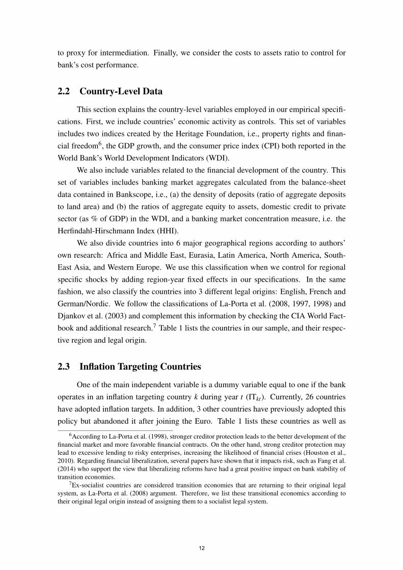
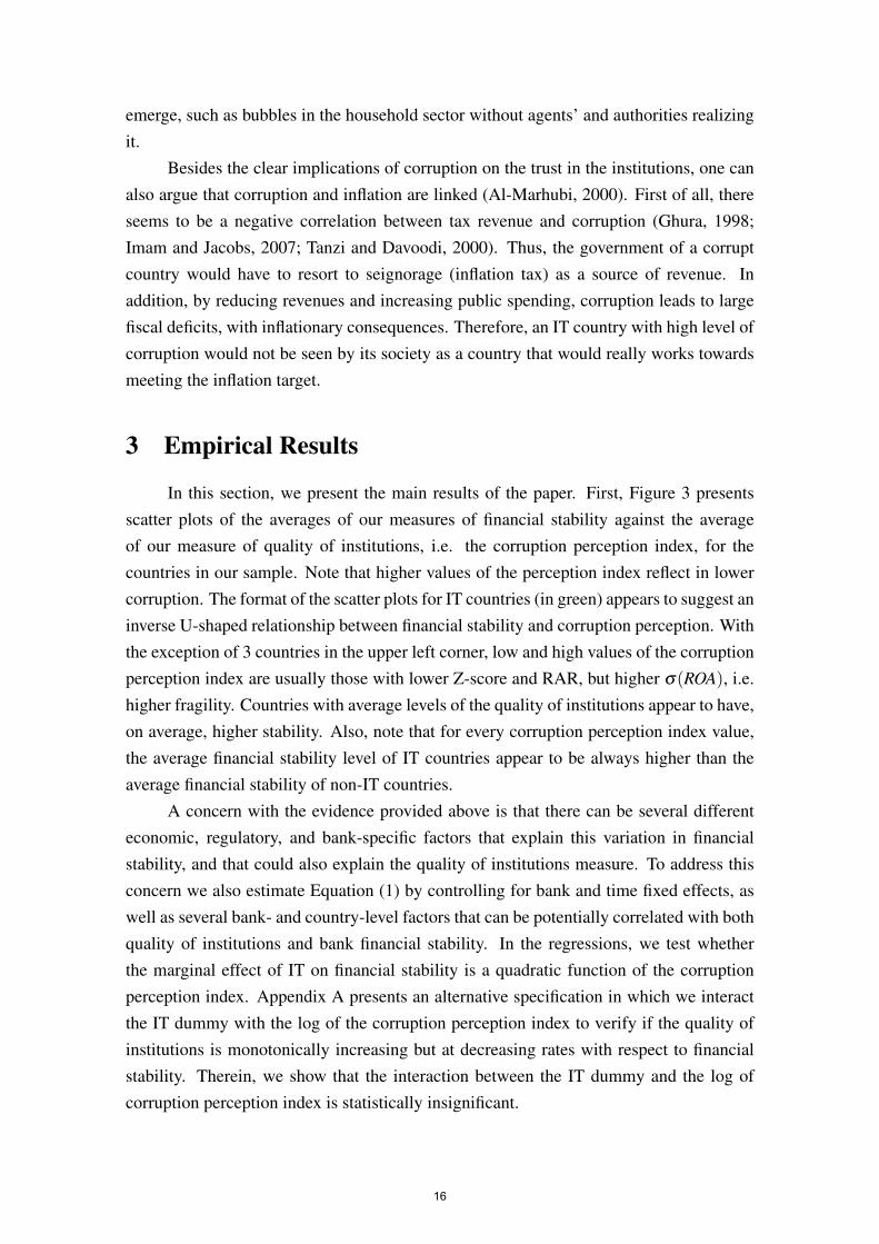
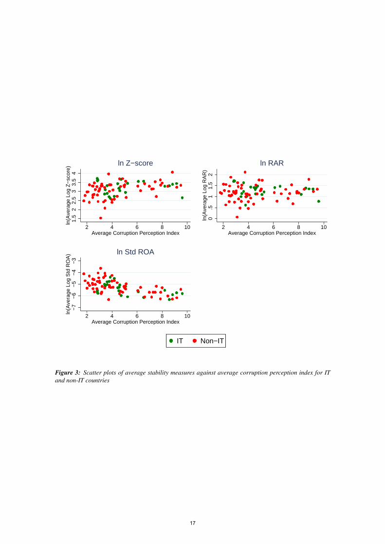
In this section, we present the main results of the paper. First, Figure 3 presentsscatter plots of the averages of our measures of financial stability against the averageof our measure of quality of institutions, i.e. the corruption perception index, for thecountries in our sample. Note that higher values of the perception index reflect in lowercorruption. The format of the scatter plots for IT countries (in green) appears to suggest aninverse U-shaped relationship between financial stability and corruption perception. Withthe exception of 3 countries in the upper left corner, low and high values of the corruptionperception index are usually those with lower Z-score and RAR, but higher σ(ROA), i.e.higher fragility. Countries with average levels of the quality of institutions appear to have,on average, higher stability. Also, note that for every corruption perception index value,the average financial stability level of IT countries appear to be always higher than theaverage financial stability of non-IT countries.

A concern with the evidence provided above is that there can be several differenteconomic, regulatory, and bank-specific factors that explain this variation in financialstability, and that could also explain the quality of institutions measure. To address thisconcern we also estimate Equation (1) by controlling for bank and time fixed effects, aswell as several bank- and country-level factors that can be potentially correlated with bothquality of institutions and bank financial stability. In the regressions, we test whetherthe marginal effect of IT on financial stability is a quadratic function of the corruptionperception index. Appendix A presents an alternative specification in which we interactthe IT dummy with the log of the corruption perception index to verify if the quality ofinstitutions is monotonically increasing but at decreasing rates with respect to financialstability. Therein, we show that the interaction between the IT dummy and the log ofcorruption perception index is statistically insignificant.

16

1.5

22.

53

3.5

4ln

(Ave

rage

Log

Z−

scor

e)

2 4 6 8 10Average Corruption Perception Index

ln Z−score

0.5

11.

52

ln(A

vera

ge L

og R

AR

)


ln RAR

−7

−6

−5

−4

−3

ln(A

vera

ge L

og S

td R

OA

)


ln Std ROA

IT Non−IT

Figure 3: Scatter plots of average stability measures against average corruption perception index for ITand non-IT countries

17

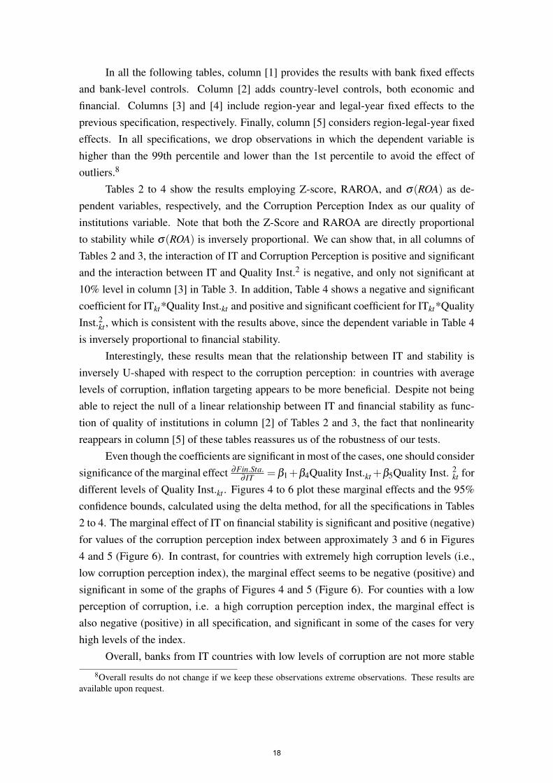
In all the following tables, column [1] provides the results with bank fixed effectsand bank-level controls. Column [2] adds country-level controls, both economic andfinancial. Columns [3] and [4] include region-year and legal-year fixed effects to theprevious specification, respectively. Finally, column [5] considers region-legal-year fixedeffects. In all specifications, we drop observations in which the dependent variable ishigher than the 99th percentile and lower than the 1st percentile to avoid the effect ofoutliers.8

Tables 2 to 4 show the results employing Z-score, RAROA, and σ(ROA) as de-pendent variables, respectively, and the Corruption Perception Index as our quality ofinstitutions variable. Note that both the Z-Score and RAROA are directly proportionalto stability while σ(ROA) is inversely proportional. We can show that, in all columns ofTables 2 and 3, the interaction of IT and Corruption Perception is positive and significantand the interaction between IT and Quality Inst.2 is negative, and only not significant at10% level in column [3] in Table 3. In addition, Table 4 shows a negative and significantcoefficient for ITkt*Quality Inst.kt and positive and significant coefficient for ITkt*QualityInst.2kt , which is consistent with the results above, since the dependent variable in Table 4is inversely proportional to financial stability.

Interestingly, these results mean that the relationship between IT and stability isinversely U-shaped with respect to the corruption perception: in countries with averagelevels of corruption, inflation targeting appears to be more beneficial. Despite not beingable to reject the null of a linear relationship between IT and financial stability as func-tion of quality of institutions in column [2] of Tables 2 and 3, the fact that nonlinearityreappears in column [5] of these tables reassures us of the robustness of our tests.

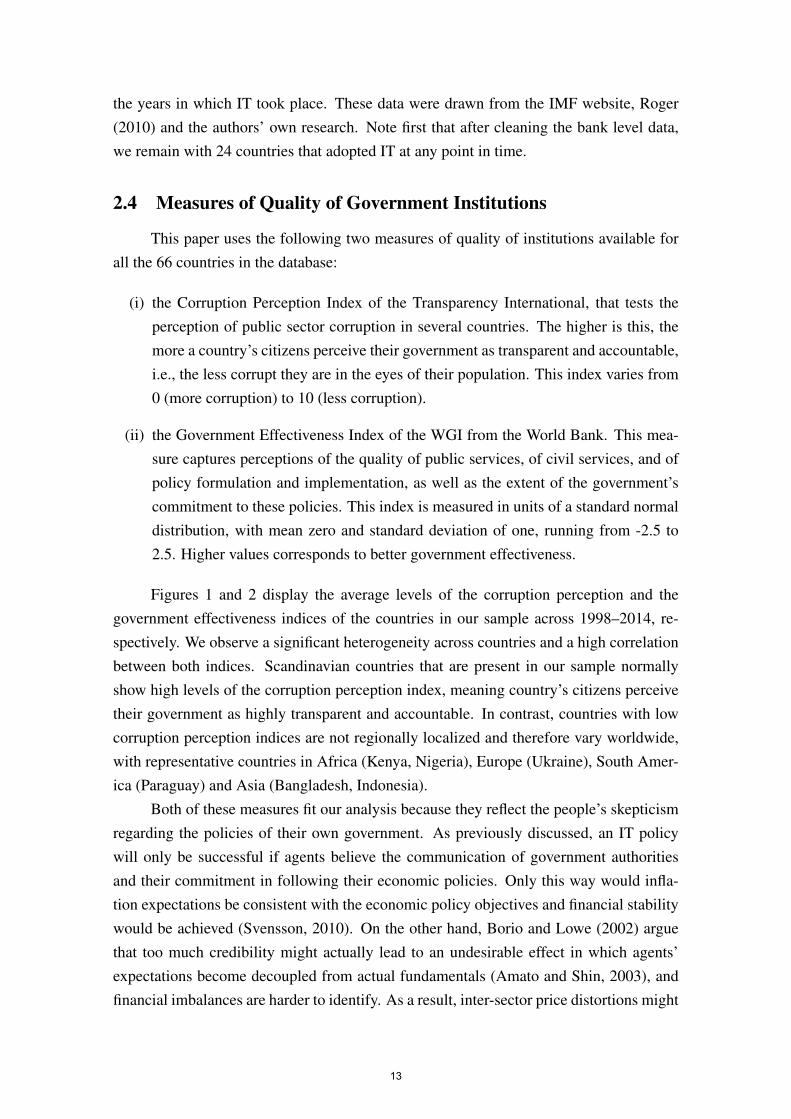
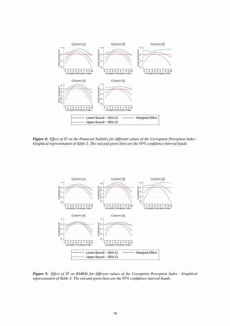
Even though the coefficients are significant in most of the cases, one should considersignificance of the marginal effect ∂Fin.Sta.

∂ IT = β1+β4Quality Inst.kt +β5Quality Inst. 2kt for

different levels of Quality Inst.kt . Figures 4 to 6 plot these marginal effects and the 95%confidence bounds, calculated using the delta method, for all the specifications in Tables2 to 4. The marginal effect of IT on financial stability is significant and positive (negative)for values of the corruption perception index between approximately 3 and 6 in Figures4 and 5 (Figure 6). In contrast, for countries with extremely high corruption levels (i.e.,low corruption perception index), the marginal effect seems to be negative (positive) andsignificant in some of the graphs of Figures 4 and 5 (Figure 6). For counties with a lowperception of corruption, i.e. a high corruption perception index, the marginal effect isalso negative (positive) in all specification, and significant in some of the cases for veryhigh levels of the index.

Overall, banks from IT countries with low levels of corruption are not more stable

8Overall results do not change if we keep these observations extreme observations. These results areavailable upon request.

18

−2

−1

01

δ ln

(Z−

Sco

re)/

δ IT

0 1 2 3 4 5 6 7 8 9 10Corruption Perception Index

Column [1]

−2

−1

01

δ ln

(Z−

Sco

re)/

δ IT


Column [2]

−2

−1

01

δ ln

(Z−

Sco

re)/

δ IT


Column [3]

−2

−1.

5−

1−

.50

.5δ

ln(Z

−S

core

)/ δ

IT


Column [4]

−3

−2

−1

01

δ ln

(Z−

Sco

re)/

δ IT


Column [5]

Lower Bound − 95% CI Marginal EffectUpper Bound − 95% CI

Figure 4: Effect of IT on the Financial Stability for different values of the Corruption Perception Index -Graphical representation of Table 2. The red and green lines are the 95% confidence interval bands.

−3

−2

−1

01

δ ln

(RA

R)/

δ IT


Column [1]

−2

−1.

5−

1−

.50

.5δ

ln(R

AR

)/ δ

IT


Column [2]

−1.

5−

1−

.50

.5δ

ln(R

AR

)/ δ

IT


Column [3]

−3

−2

−1

01

δ ln

(RA

R)/

δ IT


Column [4]

−3

−2

−1

01

δ ln

(RA

R)/

δ IT


Column [5]


Figure 5: Effect of IT on RAROA for different values of the Corruption Perception Index - Graphicalrepresentation of Table 3. The red and green lines are the 95% confidence interval bands.

19

−1

01

2δ

ln(S

TD

RO

A)/

δ IT


Column [1]

−1

01

2δ

ln(S

TD

RO

A)/

δ IT


Column [2]

−1

01

2δ

ln(S

TD

RO

A)/

δ IT


Column [3]

−1

01

2δ

ln(S

TD

RO

A)/

δ IT


Column [4]

−.5

0.5

11.

52

δ ln

(ST

D R

OA

)/ δ

IT0 1 2 3 4 5 6 7 8 9 10Corruption Perception Index

Column [5]


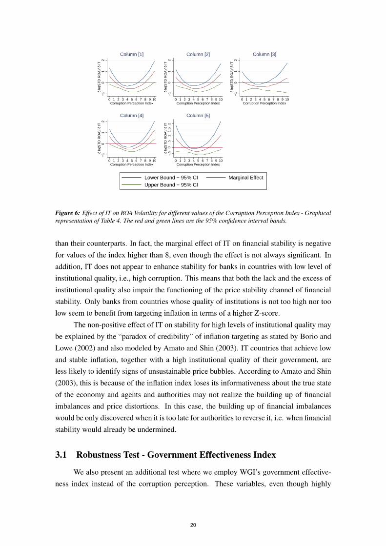
Figure 6: Effect of IT on ROA Volatility for different values of the Corruption Perception Index - Graphicalrepresentation of Table 4. The red and green lines are the 95% confidence interval bands.

than their counterparts. In fact, the marginal effect of IT on financial stability is negativefor values of the index higher than 8, even though the effect is not always significant. Inaddition, IT does not appear to enhance stability for banks in countries with low level ofinstitutional quality, i.e., high corruption. This means that both the lack and the excess ofinstitutional quality also impair the functioning of the price stability channel of financialstability. Only banks from countries whose quality of institutions is not too high nor toolow seem to benefit from targeting inflation in terms of a higher Z-score.

The non-positive effect of IT on stability for high levels of institutional quality maybe explained by the “paradox of credibility” of inflation targeting as stated by Borio andLowe (2002) and also modeled by Amato and Shin (2003). IT countries that achieve lowand stable inflation, together with a high institutional quality of their government, areless likely to identify signs of unsustainable price bubbles. According to Amato and Shin(2003), this is because of the inflation index loses its informativeness about the true stateof the economy and agents and authorities may not realize the building up of financialimbalances and price distortions. In this case, the building up of financial imbalanceswould be only discovered when it is too late for authorities to reverse it, i.e. when financialstability would already be undermined.

3.1 Robustness Test - Government Effectiveness Index

We also present an additional test where we employ WGI’s government effective-ness index instead of the corruption perception. These variables, even though highly

20

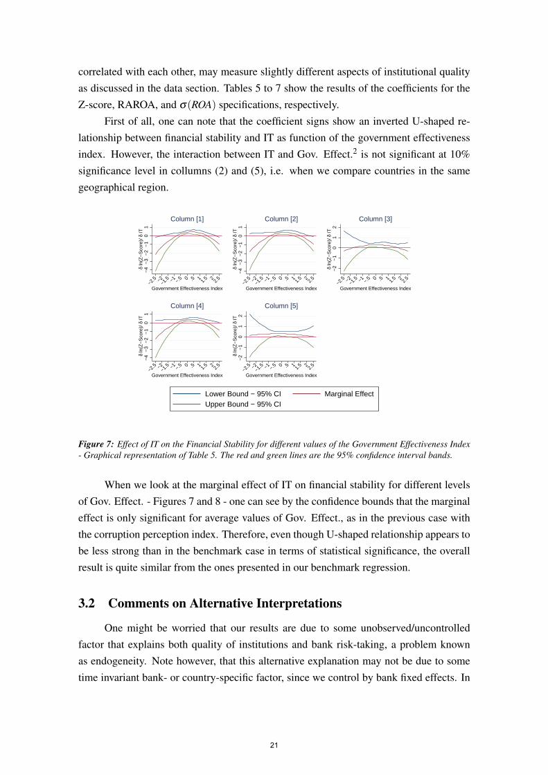
correlated with each other, may measure slightly different aspects of institutional qualityas discussed in the data section. Tables 5 to 7 show the results of the coefficients for theZ-score, RAROA, and σ(ROA) specifications, respectively.

First of all, one can note that the coefficient signs show an inverted U-shaped re-lationship between financial stability and IT as function of the government effectivenessindex. However, the interaction between IT and Gov. Effect.2 is not significant at 10%significance level in collumns (2) and (5), i.e. when we compare countries in the samegeographical region.

−4

−3

−2

−1

01

δ ln

(Z−

Sco

re)/

δ IT

−2.5 −2

−1.5 −1 −.

5 0 .5 11.

5 22.

5

Government Effectiveness Index

Column [1]

−4

−3

−2

−1

01

δ ln

(Z−

Sco

re)/

δ IT

−2.5 −2

−1.5 −1 −.

5 0 .5 11.

5 22.

5


Column [2]

−2

−1

01

2δ

ln(Z

−S

core

)/ δ

IT

−2.5 −2

−1.5 −1 −.

5 0 .5 11.

5 22.

5


Column [3]

−4

−3

−2

−1

01

δ ln

(Z−

Sco

re)/

δ IT

−2.5 −2

−1.5 −1 −.

5 0 .5 11.

5 22.

5


Column [4]

−2

−1

01

2δ

ln(Z

−S

core

)/ δ

IT

−2.5 −2

−1.5 −1 −.

5 0 .5 11.

5 22.

5


Column [5]


Figure 7: Effect of IT on the Financial Stability for different values of the Government Effectiveness Index- Graphical representation of Table 5. The red and green lines are the 95% confidence interval bands.

When we look at the marginal effect of IT on financial stability for different levelsof Gov. Effect. - Figures 7 and 8 - one can see by the confidence bounds that the marginaleffect is only significant for average values of Gov. Effect., as in the previous case withthe corruption perception index. Therefore, even though U-shaped relationship appears tobe less strong than in the benchmark case in terms of statistical significance, the overallresult is quite similar from the ones presented in our benchmark regression.

3.2 Comments on Alternative Interpretations

One might be worried that our results are due to some unobserved/uncontrolledfactor that explains both quality of institutions and bank risk-taking, a problem knownas endogeneity. Note however, that this alternative explanation may not be due to sometime invariant bank- or country-specific factor, since we control by bank fixed effects. In

21

−4

−2

02

δ ln

(RA

R)/

δ IT

−2.5 −2

−1.5 −1 −.

5 0 .5 11.

5 22.

5


Column [1]

−6

−4

−2

02

δ ln

(RA

R)/

δ IT

−2.5 −2

−1.5 −1 −.

5 0 .5 11.

5 22.

5


Column [2]

−3

−2

−1

01

δ ln

(RA

R)/

δ IT

−2.5 −2

−1.5 −1 −.

5 0 .5 11.

5 22.

5


Column [3]

−6

−4

−2

0δ

ln(R

AR

)/ δ

IT

−2.5 −2

−1.5 −1 −.

5 0 .5 11.

5 22.

5


Column [4]

−4

−3

−2

−1

01

δ ln

(RA

R)/

δ IT

−2.5 −2

−1.5 −1 −.

5 0 .5 11.

5 22.

5


Column [5]


Figure 8: Effect of IT on RAROA for different values of the Government Effectiveness Index - Graphicalrepresentation of Table 6. The red and green lines are the 95% confidence interval bands.

−1

01

23

4δ

ln(S

TD

RO

A)/

δ IT

−2.5 −2

−1.5 −1 −.

5 0 .5 11.

5 22.

5


Column [1]

−1

01

23

4δ

ln(S

TD

RO

A)/

δ IT

−2.5 −2

−1.5 −1 −.

5 0 .5 11.

5 22.

5


Column [2]

−1

01

2δ

ln(S

TD

RO

A)/

δ IT

−2.5 −2

−1.5 −1 −.

5 0 .5 11.

5 22.

5


Column [3]

−1

01

23

4δ

ln(S

TD

RO

A)/

δ IT

−2.5 −2

−1.5 −1 −.

5 0 .5 11.

5 22.

5


Column [4]

−2

−1

01

2δ

ln(S

TD

RO

A)/

δ IT

−2.5 −2

−1.5 −1 −.

5 0 .5 11.

5 22.

5


Column [5]


Figure 9: Effect of IT on ROA Volatility for different values of the Government Effectiveness Index - Graph-ical representation of Table 7. The red and green lines are the 95% confidence interval bands.

22

addition, it cannot be an alternative story that is actually correlated with country time-varying economic or financial development indicators, since we also control for them andthe results seem to hold. Finally, it cannot be some time-varying region- or legal origin-specific explanation as well.

In fact, the only alternative explanation might be a time-varying bank- or country-specific factor that is not correlated with economic and financial development variables.For instance, the population of one country could suddenly become more pessimisticregarding both the government and the economy, which would increase their perceivedcorruption at the same time as depressing the financial stability in a systematic manner.Due to the lack of data for most countries in our database, we cannot test this hypothesisempirically by also controlling for a variable that reflect the confidence of the population.We, however, believe this alternative explanation is unlikely to be the case. Our results,therefore, appear to be the most reasonable inference about the relationship between fi-nancial stability and the IT policy as a function of quality of institutions.

4 Conclusion

This paper presents new evidence on the relationship between IT and financial sta-bility. Several specialists have recently blamed IT as being too focused on reducing in-flation instead of also paying attention to asset prices. We take data from banks of 66different countries for the period of 1998-2014 and compare how institutional quality asperceived by the national population impacts financial stability in countries that adoptedIT with those that did not. In this cross-country analysis, we find an inverted U-shapedrelationship between IT and financial stability as function of the institutional quality.

References

Adrian, T. and Brunnermeier, M. K. (2016). CoVaR. American Economic Review,106(7):1705–41.

Al-Marhubi, F. A. (2000). Corrution and inflation. Economic Letters, 66(2):199–202.

Amato, J. D. and Shin, H. S. (2003). Public and private information in monetary policymodels. Bis Working Papers, 138.

Backus, D. and Driffill, J. (1984). Rational expectations and policy credibility followinga change in regime. Review of Economic Studies, 52:211–221.

Bertrand, M., Duflo, E., and Mullainathan, S. (2004). How much should we

23

trust differences-in-differences estimates? The Quarterly Journal of Economics,119(1):249–275.

Blanchard, O., Dell’Ariccia, G., and Mauro, P. (2010). Rethinking macroeconomic policy.IMF Staff Position Note.

Bodea, C. and Hicks, R. (2015). Price stability and central bank independence: Discipline,credibility, and democratic institutions. International Organization, 69(1):35–61.

Bordo, M. D. and Wheelock, D. W. (1998). Price stability and financial stability: Thehistorical record. Federal Reserve Bank of St Louis Review, September/October:41–62.

Borio, C. (2005). Monetary and financial stability: So close and yet so far. National

Institute Economic Review, 192(1):84–101.

Borio, C. (2006). Monetary and financial stability: Here to stay? Journal of Banking &

Finance, 30(12):3407–3414.

Borio, C. and Lowe, P. (2002). Asset prices, financial and monetary stability: exploringthe nexus. BIS Working Papers, 14.

Bos, J. W. B. and Koetter, M. (2009). Handling losses in translog profit models. Applied

Economics, 41:1466–1483.

Boyd, J. H. and Runkle, D. E. (1993). Size and performance of banking firms: Testingthe predictions of theory. Journal of Monetary Economics, 31(1):47–67.

Chiaramonte, L., Liu, F. H., Poli, F., and Zhou, M. (2016). How accurately can Z-scorepredict bank failure? Financial Markets, Institutions and Instruments, 25(5):333–360.

Demirguc-Kunt, A. and Huizinga, H. (2010). Bank activity and funding strategies: Theimpact on risk and returns. Journal of Financial Economics, 98:626–650.

Dincer, N. N. and Eichengreen, B. (2014). Central bank transparency and independence:Updates and new measures. International Journal of Central Banking, 10(1):189–259.

Djankov, S., La-Porta, R., de Silanes, F. L., and Shleifer, A. (2003). Courts. The Quarterly

Journal of Economics, 118(2):453–517.

Donald, S. G. and Lang, K. (2007). Inference with difference-in-difference and otherpanel data. The Review of Economics and Statistics, 89(2):221–233.

Fang, Y., Hasan, I., and Marton, K. (2014). Institutional development and bank stability:Evidence from transition countries. Journal of Banking & Finance, 39:160–176.

24

Fazio, D. M., Tabak, B. M., and Cajueiro, D. O. (2015). Inflation targeting: Is IT to blamefor banking system instability? Journal of Banking & Finance, 59:76–97.

Fiordelisi, F. and Mare, D. S. (2014). Competition and financial stability in Europeancooperative banks. Journal of International Money and Finance, 45(Supplement C):1–16.

Fouejieu, A. (2017). Inflation targeting and financial stability in emerging markets. Eco-

nomic Modelling, 60:51–70.

Fu, X., Lin, Y., and Molyneux, P. (2014). Bank competition and financial stability in AsiaPacific. Journal of Banking and Finance, 38(Supplement C):64–77.

Ghura, D. (1998). Tax revenue in sub-Saharan Africa: effects of economic policies andcorruption. IMF Working Paper No. 135.

Heenan, G., Peter, M., and Roger, S. (2006). Implementing inflation targeting: Institu-tional arrangements, target design, and communication. IMF Working Paper 06/278.

Houston, J. F., Lin, C., Lin, P., and Ma, Y. (2010). Creditor rights, information sharing,and bank risk taking. Journal of Financial Economics, 96:485–512.

Hove, S., Tchana, F. T., and Mama, A. T. (2017). Do monetary, fiscal and financial insti-tutions really matter for inflation targeting in emerging market economies? Research

in International Business and Finance, 39, Part A:128–149.

Imam, P. A. and Jacobs, D. F. (2007). Effect of corruption on tax revenues in the Middle-East. IMF Working Paper No. 270.

Kim, S. and Mehrotra, A. (2017). Managing price and financial stability objectives ininflation targeting economies in Asia and the Pacific. Journal of Financial Stability.DOI: http://dx.doi.org/10.1016/j.jfs.2017.01.003.

Klomp, J. and de Haan, J. (2014). Bank regulation, the quality of institutions, and bankingrisk in emerging and developing countries: An empirical analysis. Emerging Markets

Finance and Trade, 50(6):19–40.

La-Porta, R., de Silanes, F. L., and Shleifer, A. (2008). The economic consequences oflegal origins. Journal of Economic Literature, 46(2):285–332.

La-Porta, R., Lopez-De-Silanes, F., Shleifer, A., and Vishny, R. W. (1997). Legal deter-minants of external finance. The Journal of Finance, 52(3):1131–1150.

La-Porta, R., Lopez-De-Silanes, F., Shleifer, A., and Vishny, R. W. (1998). Law andfinance. Journal of Political Economy, 106(6):1113–1155.

25

Laeven, L. and Levine, R. (2009). Bank governance, regulation and risk taking. Journal

of Financial Economics, 93:259–275.

Lozano-Vivas, A. and Pasiouras, F. (2010). The impact of non-traditional activities on theestimation of bank efficiency: International evidence. Journal of Banking & Finance,33:1436–1449.

Mercieca, S., Schaeck, K., and Wolfe, S. (2007). Small European banks: Benefits fromdiversification? Journal of Banking & Finance, 31(7):1975–1998.

Mishkin, F. (2004). Can inflation targeting work in emerging market countries? NBER

Working Papers 10646.

Montes, G. C. and Peixoto, G. B. T. (2014). Risk-taking channel, bank lending channeland the “paradox of credibility”: Evidence from Brazil. Economic Modelling, 39:82–94.

Roger, S. (2010). Inflation targeting turns 20. Finance & Development, 47(1):46–49.

Roy, A. D. (1952). Safety first and the holding of assets. Econometrica, 20:431–449.

Ruge-Murcia, F. J. (1995). Credibility and changes in policy regime. Journal of Political

Economy, 103(1):176–208.

Schwartz, A. J. (1995). Why financial stability depends on price stability. Economic

Affairs, 15(4):21–25.

Svensson, L. E. O. (2010). Inflation targeting. NBER Working Paper No. 16654.

Tanzi, V. and Davoodi, H. R. (2000). Corruption, growth, and public finances. IMF

Working Paper No. 182.

A Alternative specification

Tables 8 to 10 present alternative specifications in which we interact the IT dummywith the log of the corruption perception index. This specification tests whether the IT-financial stability relationship is a log function of the corruption perception index, insteadof a quadratic function as found in our main specifications. Note that our main result isnot inconsistent with the fact that the relationship is actually increasing but at lower ratesin a log fashion. Both explanations require the first derivative of financial stability overcorruption to be positive, and the second derivative to be negative. Table 8 to 10, however,appear to disprove this alternative explanation: the interaction of IT with the log of the

26

corruption index is positive in Tables 8 and 9, and negative in Table 10, but they are notsignificant. Thus, even though the sign of the coefficient might suggest a log relationshipbetween IT and financial stability as a function of our quality of institutions proxy, thisrelationship is not statistically significant for our sample of countries. This suggests thatour main inverse-U shaped result indeed appears to be a more suitable fit to the empiricaldata.

27

Tabl

e1:

Cou

ntri

es,R

egio

ns,L

egal

Ori

gins

and

Ado

ptio

nof

Infla

tion

Targ

et

Cou

ntry

Reg

ion

Leg

alO

rigi

nIT

?A

dopt

ion

Cou

ntry

Reg

ion

Leg

alO

rigi

nIT

?A

dopt

ion

GH

AN

AA

fric

a/M

EE

nglis

hY

es20

07H

UN

GA

RYE

uras

iaG

erm

anY

es20

01IS

RA

EL

Afr

ica/

ME

Eng

lish

Yes

1997

POL

AN

DE

uras

iaG

erm

anY

es19

98K

EN

YAA

fric

a/M

EE

nglis

hSL

OVA

KIA

Eur

asia

Ger

man

Yes

2005

to20

08N

IGE

RIA

Afr

ica/

ME

Eng

lish

SLO

VE

NIA

Eur

asia

Ger

man

SOU

TH

AFR

ICA

Afr

ica/

ME

Eng

lish

Yes

2000

BO

LIV

IAL

atin

Am

eric

aFr

ench

TAN

ZA

NIA

Afr

ica/

ME

Eng

lish

BR

AZ

ILL

atin

Am

eric

aFr

ench

Yes

1999

EG

YPT

Afr

ica/

ME

Fren

chC

OL

OM

BIA

Lat

inA

mer

ica

Fren

chY

es19

99JO

RD

AN

Afr

ica/

ME

Fren

chC

OST

AR

ICA

Lat

inA

mer

ica

Fren

chM

AU

RIT

IUS

Afr

ica/

ME

Fren

chD

OM

INIC

AN

RE

PUB

LIC

Lat

inA

mer

ica

Fren

chT

UN

ISIA

Afr

ica/

ME

Fren

chE

CU

AD

OR

Lat

inA

mer

ica

Fren

chT

UR

KE

YA

fric

a/M

EFr

ench

Yes

2006

EL

SALV

AD

OR

Lat

inA

mer

ica

Fren

chA

UST

RA

LIA

Eas

tAsi

aE

nglis

hY

es19

93G

UA

TE

MA

LA

Lat

inA

mer

ica

Fren

chY

es20

05B

AN

GL

AD

ESH

Eas

tAsi

aE

nglis

hM

EX

ICO

Lat

inA

mer

ica

Fren

chY

es20

01H

ON

GK

ON

GE

astA

sia

Eng

lish

PAN

AM

AL

atin

Am

eric

aFr

ench

IND

IAE

astA

sia

Eng

lish

PAR

AG

UA

YL

atin

Am

eric

aFr

ench

MA

LA

YSI

AE

astA

sia

Eng

lish

PER

UL

atin

Am

eric

aFr

ench

Yes

2002

NE

PAL

Eas

tAsi

aE

nglis

hC

AN

AD

AN

orth

Am

eric

aE

nglis

hY

es19

91PA

KIS

TAN

Eas

tAsi

aE

nglis

hU

NIT

ED

STA

TE

SN

orth

Am

eric

aE

nglis

hT

HA

ILA

ND

Eas

tAsi

aE

nglis

hY

es20

00IR

EL

AN

DW

estE

urop

eE

nglis

hIN

DO

NE

SIA

Eas

tAsi

aFr

ench

Yes

2005

UN

ITE

DK

ING

DO

MW

estE

urop

eE

nglis

hY

es19

92PH

ILIP

PIN

ES

Eas

tAsi

aFr

ench

Yes

2002

BE

LG

IUM

Wes

tEur

ope

Fren

chC

HIN

AE

astA

sia

Ger

man

FRA

NC

EW

estE

urop

eFr

ench

JAPA

NE

astA

sia

Ger

man

ITA

LYW

estE

urop

eFr

ench

KO

RE

AE

astA

sia

Ger

man

Yes

2001

LU

XE

MB

OU

RG

Wes

tEur

ope

Fren

chA

RM

EN

IAE

uras

iaFr

ench

POR

TU

GA

LW

estE

urop

eFr

ench

KA

ZA

KH

STA

NE

uras

iaFr

ench

SPA

INW

estE

urop

eFr

ench

Yes

1993

to19

98M

OL

DO

VAE

uras

iaFr

ench

AU

STR

IAW

estE

urop

eG

erm

anR

OM

AN

IAE

uras

iaFr

ench

Yes

2005

DE

NM

AR

KW

estE

urop

eG

erm

anR

USS

IAE

uras

iaFr

ench

FIN

LA

ND

Wes

tEur

ope

Ger

man

Yes

1995

to19

98U

KR

AIN

EE

uras

iaFr

ench

GE

RM

AN

YW

estE

urop

eG

erm

anB

UL

GA

RIA

Eur

asia

Ger

man

LA

TV

IAW

estE

urop

eG

erm

anC

RO

AT

IAE

uras

iaG

erm

anSW

ED

EN

Wes

tEur

ope

Ger

man

Yes

1993

CZ

EC

HR

EPU

BL

ICE

uras

iaG

erm

anY

es19

97SW

ITZ

ER

LA

ND

Wes

tEur

ope

Ger

man

28

Table 2: Corruption Perception Index + ITkt : Z-score Equation

This table presents the fixed-effects regression of a measure of financial stability (the natural log of theZ-score) against a set of control variables, a dummy of inflation targeting and a variable that measuresthe corruption perception of a country. Higher values for this index mean lower corruption. This variablewas taken from Transparency International. The subscript t refers to years, i to banks, and k to countries.Country-specific controls include Financial Depth controls include the density of deposits, the equity toassets ratio (aggregated), the HHI of assets, and the domestic credit provided to the financial sector (as %of the GDP), the GDP cycle (derived from HP filters of each country’s log of GDP), the consumer priceindex (CPI) the Financial Freedom Index and the Property Rights Index. We also include balance sheetvariables such as SIZEikt , Liquidity Ratio and Cost To Assets ratio. In all estimations, the upper and lowerpercentiles of the dependent variable are not considered. Robust standard errors clustered by country inparentheses.**** p<0.01, ** p<0.05, * p<0.1

(1) (2) (3) (4) (5)VARIABLES ln(Z-scoreikt ) ln(Z-scoreikt ) ln(Z-scoreikt ) ln(Z-scoreikt ) ln(Z-scoreikt )

ITkt -0.695* -0.636* -0.248 -0.822** -0.719(0.401) (0.373) (0.458) (0.351) (0.585)

ITkt*Quality Inst.kt 0.521*** 0.487*** 0.237 0.560*** 0.439*(0.176) (0.166) (0.197) (0.152) (0.239)

ITkt*Quality Inst.2kt -0.057*** -0.052*** -0.026 -0.062*** -0.048**(0.016) (0.015) (0.019) (0.014) (0.022)

Quality Inst.kt -0.193 -0.107 0.120 -0.034 0.046(0.190) (0.135) (0.114) (0.115) (0.146)

Quality Inst.2kt 0.030* 0.020* -0.005 0.018* 0.016(0.017) (0.011) (0.011) (0.011) (0.015)

Bank FE Yes Yes Yes Yes YesBank Controls Yes Yes Yes Yes YesCountry Controls Yes Yes Yes YesRegion x Year FE YesLegal Origin x Year FE YesRegion x Legal Origin x Year FE Yes

Observations 98,458 98,458 98,458 98,458 98,458R-squared 0.575 0.577 0.582 0.579 0.585

29

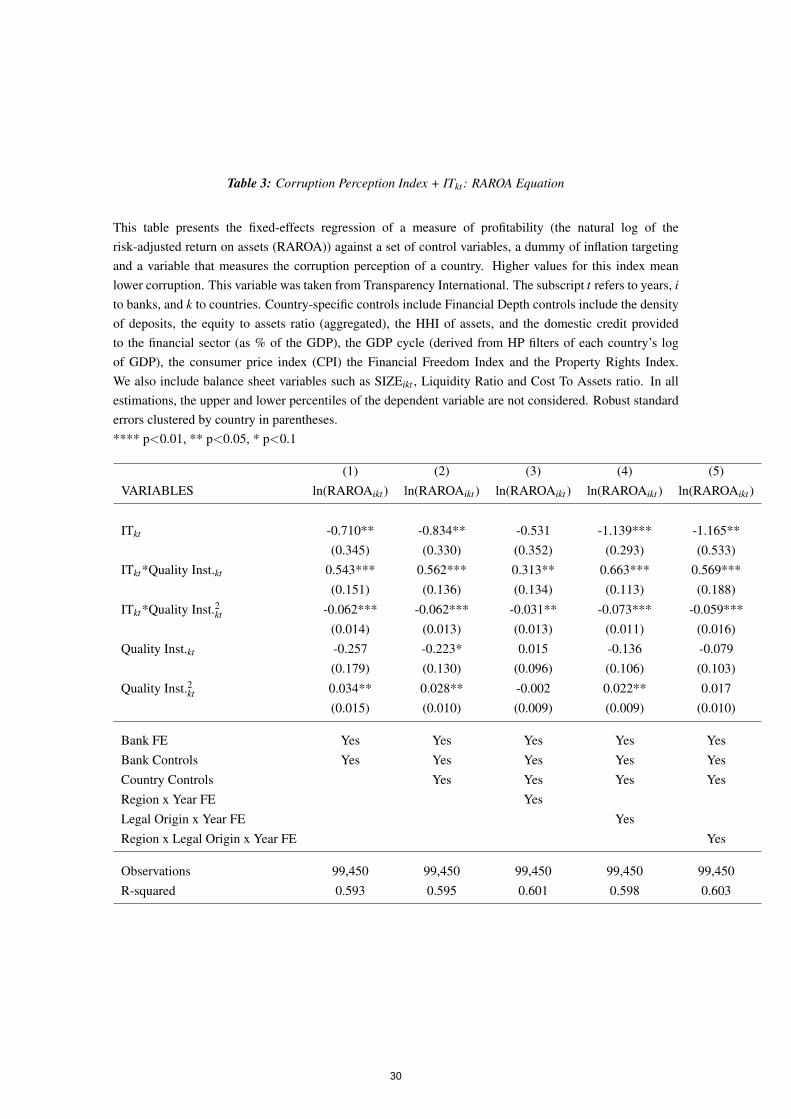
Table 3: Corruption Perception Index + ITkt : RAROA Equation

This table presents the fixed-effects regression of a measure of profitability (the natural log of therisk-adjusted return on assets (RAROA)) against a set of control variables, a dummy of inflation targetingand a variable that measures the corruption perception of a country. Higher values for this index meanlower corruption. This variable was taken from Transparency International. The subscript t refers to years, ito banks, and k to countries. Country-specific controls include Financial Depth controls include the densityof deposits, the equity to assets ratio (aggregated), the HHI of assets, and the domestic credit providedto the financial sector (as % of the GDP), the GDP cycle (derived from HP filters of each country’s logof GDP), the consumer price index (CPI) the Financial Freedom Index and the Property Rights Index.We also include balance sheet variables such as SIZEikt , Liquidity Ratio and Cost To Assets ratio. In allestimations, the upper and lower percentiles of the dependent variable are not considered. Robust standarderrors clustered by country in parentheses.**** p<0.01, ** p<0.05, * p<0.1

(1) (2) (3) (4) (5)VARIABLES ln(RAROAikt ) ln(RAROAikt ) ln(RAROAikt ) ln(RAROAikt ) ln(RAROAikt )

ITkt -0.710** -0.834** -0.531 -1.139*** -1.165**(0.345) (0.330) (0.352) (0.293) (0.533)

ITkt*Quality Inst.kt 0.543*** 0.562*** 0.313** 0.663*** 0.569***(0.151) (0.136) (0.134) (0.113) (0.188)

ITkt*Quality Inst.2kt -0.062*** -0.062*** -0.031** -0.073*** -0.059***(0.014) (0.013) (0.013) (0.011) (0.016)

Quality Inst.kt -0.257 -0.223* 0.015 -0.136 -0.079(0.179) (0.130) (0.096) (0.106) (0.103)

Quality Inst.2kt 0.034** 0.028** -0.002 0.022** 0.017(0.015) (0.010) (0.009) (0.009) (0.010)



30

Table 4: Corruption Perception Index + ITkt : σ (ROA) Equation

This table presents the fixed-effects regression of a measure of ROA Volatility (the natural log of σ (ROA))against a set of control variables, a dummy of inflation targeting and a variable that measures the corruptionperception of a country. Higher values for this index mean lower corruption. This variable was taken fromTransparency International. Country-specific controls include Financial Depth controls include the densityof deposits, the equity to assets ratio (aggregated), the HHI of assets, and the domestic credit providedto the financial sector (as % of the GDP), the GDP cycle (derived from HP filters of each country’s logof GDP), the consumer price index (CPI) the Financial Freedom Index and the Property Rights Index.We also include balance sheet variables such as SIZEikt , Liquidity Ratio and Cost To Assets ratio. In allestimations, the upper and lower percentiles of the dependent variable are not considered. Robust standarderrors clustered by country in parentheses.**** p<0.01, ** p<0.05, * p<0.1

(1) (2) (3) (4) (5)VARIABLES ln(σ (ROA)ikt ) ln(σ (ROA)ikt ) ln(σ (ROA)ikt ) ln(σ (ROA)ikt ) ln(σ (ROA)ikt )

ITkt 0.596 0.459 0.075 0.655* 0.767(0.365) (0.365) (0.451) (0.339) (0.571)

ITkt*Quality Inst.kt -0.491*** -0.425*** -0.200 -0.501*** -0.471*(0.158) (0.160) (0.197) (0.147) (0.237)

ITkt*Quality Inst.2kt 0.053*** 0.046*** 0.023 0.056*** 0.050**(0.014) (0.015) (0.019) (0.014) (0.022)

Quality Inst.kt 0.206 0.108 -0.093 0.031 -0.012(0.176) (0.134) (0.134) (0.124) (0.164)

Quality Inst.2kt -0.028* -0.018 0.005 -0.016 -0.018(0.016) (0.011) (0.013) (0.011) (0.016)



31

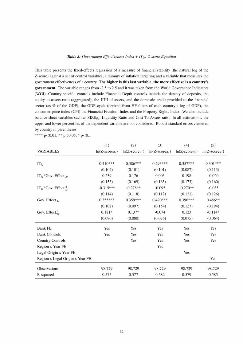
Table 5: Government Effectiveness Index + ITkt : Z-score Equation

This table presents the fixed-effects regression of a measure of financial stability (the natural log of theZ-score) against a set of control variables, a dummy of inflation targeting and a variable that measures thegovernment effectiveness of a country. The higher is this last variable, the more effective is a country’sgovernment. The variable ranges from -2.5 to 2.5 and it was taken from the World Governance Indicators(WGI). Country-specific controls include Financial Depth controls include the density of deposits, theequity to assets ratio (aggregated), the HHI of assets, and the domestic credit provided to the financialsector (as % of the GDP), the GDP cycle (derived from HP filters of each country’s log of GDP), theconsumer price index (CPI) the Financial Freedom Index and the Property Rights Index. We also includebalance sheet variables such as SIZEikt , Liquidity Ratio and Cost To Assets ratio. In all estimations, theupper and lower percentiles of the dependent variable are not considered. Robust standard errors clusteredby country in parentheses.**** p<0.01, ** p<0.05, * p<0.1


ITkt 0.410*** 0.386*** 0.293*** 0.357*** 0.301***(0.104) (0.101) (0.101) (0.087) (0.113)

ITkt*Gov. Effect.kt 0.239 0.176 0.003 0.198 -0.020(0.153) (0.169) (0.165) (0.173) (0.160)

ITkt*Gov. Effect.2kt -0.315*** -0.278** -0.095 -0.270** -0.035(0.114) (0.118) (0.112) (0.121) (0.126)

Gov. Effect.kt 0.355*** 0.359*** 0.420*** 0.396*** 0.486**(0.102) (0.097) (0.154) (0.127) (0.194)

Gov. Effect.2kt 0.181* 0.137* -0.074 0.123 -0.114*(0.096) (0.080) (0.076) (0.075) (0.064)



32

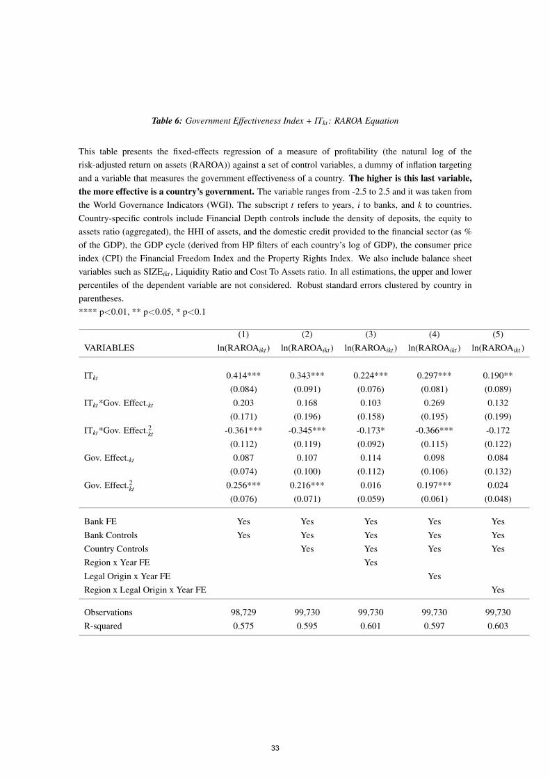
Table 6: Government Effectiveness Index + ITkt : RAROA Equation

This table presents the fixed-effects regression of a measure of profitability (the natural log of therisk-adjusted return on assets (RAROA)) against a set of control variables, a dummy of inflation targetingand a variable that measures the government effectiveness of a country. The higher is this last variable,the more effective is a country’s government. The variable ranges from -2.5 to 2.5 and it was taken fromthe World Governance Indicators (WGI). The subscript t refers to years, i to banks, and k to countries.Country-specific controls include Financial Depth controls include the density of deposits, the equity toassets ratio (aggregated), the HHI of assets, and the domestic credit provided to the financial sector (as %of the GDP), the GDP cycle (derived from HP filters of each country’s log of GDP), the consumer priceindex (CPI) the Financial Freedom Index and the Property Rights Index. We also include balance sheetvariables such as SIZEikt , Liquidity Ratio and Cost To Assets ratio. In all estimations, the upper and lowerpercentiles of the dependent variable are not considered. Robust standard errors clustered by country inparentheses.**** p<0.01, ** p<0.05, * p<0.1


ITkt 0.414*** 0.343*** 0.224*** 0.297*** 0.190**(0.084) (0.091) (0.076) (0.081) (0.089)

ITkt*Gov. Effect.kt 0.203 0.168 0.103 0.269 0.132(0.171) (0.196) (0.158) (0.195) (0.199)

ITkt*Gov. Effect.2kt -0.361*** -0.345*** -0.173* -0.366*** -0.172(0.112) (0.119) (0.092) (0.115) (0.122)

Gov. Effect.kt 0.087 0.107 0.114 0.098 0.084(0.074) (0.100) (0.112) (0.106) (0.132)

Gov. Effect.2kt 0.256*** 0.216*** 0.016 0.197*** 0.024(0.076) (0.071) (0.059) (0.061) (0.048)



33

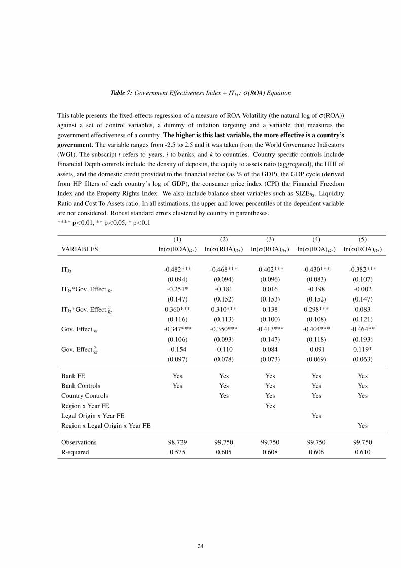
Table 7: Government Effectiveness Index + ITkt : σ (ROA) Equation

This table presents the fixed-effects regression of a measure of ROA Volatility (the natural log of σ (ROA))against a set of control variables, a dummy of inflation targeting and a variable that measures thegovernment effectiveness of a country. The higher is this last variable, the more effective is a country’sgovernment. The variable ranges from -2.5 to 2.5 and it was taken from the World Governance Indicators(WGI). The subscript t refers to years, i to banks, and k to countries. Country-specific controls includeFinancial Depth controls include the density of deposits, the equity to assets ratio (aggregated), the HHI ofassets, and the domestic credit provided to the financial sector (as % of the GDP), the GDP cycle (derivedfrom HP filters of each country’s log of GDP), the consumer price index (CPI) the Financial FreedomIndex and the Property Rights Index. We also include balance sheet variables such as SIZEikt , LiquidityRatio and Cost To Assets ratio. In all estimations, the upper and lower percentiles of the dependent variableare not considered. Robust standard errors clustered by country in parentheses.**** p<0.01, ** p<0.05, * p<0.1


ITkt -0.482*** -0.468*** -0.402*** -0.430*** -0.382***(0.094) (0.094) (0.096) (0.083) (0.107)

ITkt*Gov. Effect.kt -0.251* -0.181 0.016 -0.198 -0.002(0.147) (0.152) (0.153) (0.152) (0.147)

ITkt*Gov. Effect.2kt 0.360*** 0.310*** 0.138 0.298*** 0.083(0.116) (0.113) (0.100) (0.108) (0.121)

Gov. Effect.kt -0.347*** -0.350*** -0.413*** -0.404*** -0.464**(0.106) (0.093) (0.147) (0.118) (0.193)

Gov. Effect.2kt -0.154 -0.110 0.084 -0.091 0.119*(0.097) (0.078) (0.073) (0.069) (0.063)



34

Table 8: Alternative Explanation: Is the IT-stability relationship a log function of the corruption perceptionindex?

This table presents the fixed-effects regression of a measure of financial stability (the natural log of theZ-score) against a set of control variables, a dummy of inflation targeting and a variable that measures thecorruption perception of a country. Higher values for this index mean lower corruption. This variable wastaken from Transparency International. We interact the log of the Corruption Index with the IT variableto understand whether the effect of IT on financial stability is increasing, but at a lower rate as the indexincreases. The subscript t refers to years, i to banks, and k to countries. Country-specific controls includeFinancial Depth controls include the density of deposits, the equity to assets ratio (aggregated), the HHI ofassets, and the domestic credit provided to the financial sector (as % of the GDP), the GDP cycle (derivedfrom HP filters of each country’s log of GDP), the consumer price index (CPI) the Financial FreedomIndex and the Property Rights Index. We also include balance sheet variables such as SIZEikt , LiquidityRatio and Cost To Assets ratio. In all estimations, the upper and lower percentiles of the dependentvariable are not considered. Robust standard errors clustered by country in parentheses.**** p<0.01, ** p<0.05, * p<0.1


ITkt 0.093 0.119 0.061 0.144 -0.052(0.316) (0.287) (0.264) (0.350) (0.490)

ITkt*Ln(Corruption Perception)kt 0.227 0.203 0.199 0.091 0.213(0.280) (0.245) (0.223) (0.295) (0.375)

Ln(Corruption Perception)kt 0.197 0.210 0.387** 0.155 0.361*(0.251) (0.193) (0.151) (0.181) (0.216)



35

Table 9: Alternative Explanation: Is the IT-stability relationship a log function of the corruption perceptionindex? RAROA Equation

This table presents the fixed-effects regression of a measure of financial stability (the natural log of theRAROA) against a set of control variables, a dummy of inflation targeting and a variable that measures thecorruption perception of a country. Higher values for this index mean lower corruption. This variable wastaken from Transparency International. We interact the log of the Corruption Index with the IT variableto understand whether the effect of IT on financial stability is increasing, but at a lower rate as the indexincreases. The subscript t refers to years, i to banks, and k to countries. Country-specific controls includeFinancial Depth controls include the density of deposits, the equity to assets ratio (aggregated), the HHI ofassets, and the domestic credit provided to the financial sector (as % of the GDP), the GDP cycle (derivedfrom HP filters of each country’s log of GDP), the consumer price index (CPI) the Financial FreedomIndex and the Property Rights Index. We also include balance sheet variables such as SIZEikt , LiquidityRatio and Cost To Assets ratio. In all estimations, the upper and lower percentiles of the dependent variableare not considered. Robust standard errors clustered by country in parentheses.**** p<0.01, ** p<0.05, * p<0.1


ITkt 0.324 0.237 0.072 0.057 -0.129(0.395) (0.391) (0.353) (0.334) (0.512)

ITkt*Ln(Corruption Perception)kt 0.061 0.086 0.143 0.095 0.203(0.311) (0.286) (0.251) (0.248) (0.365)

Ln(Corruption Perception)kt 0.175 0.132 0.274* -0.016 0.150(0.311) (0.254) (0.150) (0.153) (0.148)



36

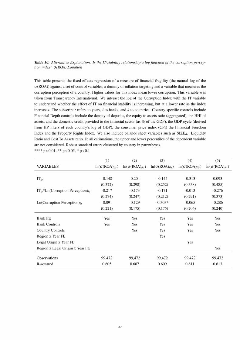
Table 10: Alternative Explanation: Is the IT-stability relationship a log function of the corruption percep-tion index? σ (ROA) Equation

This table presents the fixed-effects regression of a measure of financial fragility (the natural log of theσ (ROA)) against a set of control variables, a dummy of inflation targeting and a variable that measures thecorruption perception of a country. Higher values for this index mean lower corruption. This variable wastaken from Transparency International. We interact the log of the Corruption Index with the IT variableto understand whether the effect of IT on financial stability is increasing, but at a lower rate as the indexincreases. The subscript t refers to years, i to banks, and k to countries. Country-specific controls includeFinancial Depth controls include the density of deposits, the equity to assets ratio (aggregated), the HHI ofassets, and the domestic credit provided to the financial sector (as % of the GDP), the GDP cycle (derivedfrom HP filters of each country’s log of GDP), the consumer price index (CPI) the Financial FreedomIndex and the Property Rights Index. We also include balance sheet variables such as SIZEikt , LiquidityRatio and Cost To Assets ratio. In all estimations, the upper and lower percentiles of the dependent variableare not considered. Robust standard errors clustered by country in parentheses.**** p<0.01, ** p<0.05, * p<0.1


ITkt -0.148 -0.204 -0.144 -0.313 0.093(0.322) (0.298) (0.252) (0.338) (0.485)

ITkt*Ln(Corruption Perception)kt -0.217 -0.173 -0.171 -0.013 -0.276(0.274) (0.247) (0.212) (0.291) (0.373)

Ln(Corruption Perception)kt -0.091 -0.129 -0.303* -0.065 -0.286(0.221) (0.175) (0.175) (0.206) (0.240)



37

Dimas Mateus Fazio, Thiago Christiano Silva, Benjamin ... · Inflation Targeting and Financial...

Documents

Transcript of Dimas Mateus Fazio, Thiago Christiano Silva, Benjamin ... · Inflation Targeting and Financial...