DIIN PAP SI - IZA Institute of Labor Economicsftp.iza.org/dp10807.pdf · Courtney Ward, Mutlu...

Discussion PaPer series

IZA DP No. 10807

Mevlude Akbulut-Yuksel

War during Childhood:The Long Run Effects of Warfare on Health

mAy 2017

Any opinions expressed in this paper are those of the author(s) and not those of IZA. Research published in this series may include views on policy, but IZA takes no institutional policy positions. The IZA research network is committed to the IZA Guiding Principles of Research Integrity.The IZA Institute of Labor Economics is an independent economic research institute that conducts research in labor economics and offers evidence-based policy advice on labor market issues. Supported by the Deutsche Post Foundation, IZA runs the world’s largest network of economists, whose research aims to provide answers to the global labor market challenges of our time. Our key objective is to build bridges between academic research, policymakers and society.IZA Discussion Papers often represent preliminary work and are circulated to encourage discussion. Citation of such a paper should account for its provisional character. A revised version may be available directly from the author.

Schaumburg-Lippe-Straße 5–953113 Bonn, Germany

Phone: +49-228-3894-0Email: [email protected] www.iza.org

IZA – Institute of Labor Economics

Discussion PaPer series

IZA DP No. 10807

War during Childhood:The Long Run Effects of Warfare on Health

mAy 2017

Mevlude Akbulut-YukselDalhousie University and IZA

AbstrAct

mAy 2017IZA DP No. 10807

War during Childhood:The Long Run Effects of Warfare on Health*

This paper estimates the causal long-term consequences of an exposure to war in utero

and during childhood on the risk of obesity and the probability of having a chronic health

condition in adulthood. Using the plausibly exogenous city-by-cohort variation in the

intensity of WWII destruction as a unique quasi-experiment, I find that individuals who

were exposed to WWII destruction during the prenatal and early postnatal periods have

higher BMIs and are more likely to be obese as adults. I also find an elevated incidence

of chronic health conditions such as stroke, hypertension, diabetes, and cardiovascular

disorder in adulthood among these wartime children.

JEL Classification: I10, I12, J13

Keywords: warfare, body size, health conditions, children

Corresponding author:Mevlude Akbulut-YukselDepartment of EconomicsDalhousie UniversityHalifax, NSCanada

E-mail: [email protected]

* I am grateful to Randall Akee, Richard Akresh, Aimee Chin, De- bra Cobb-Clark, Amelie Constant, Charles Courtemanche, Adriana Kugler, Wang Sheng Lee, Jason Lindo, Shelley Phipps, Olga Shemyakina, Erdal Tekin, Courtney Ward, Mutlu Yuksel and Klaus Zimmermann, as well as seminar participants at Dalhousie University and Wesleyan University and participants at the Canadian Economic Association Meeting, the IZA Conference on Risky Behavior and the HICN Workshop in Berkeley, for their helpful comments and suggestions. All errors are my own.

I. Introduction

Globally, child malnutrition continues to be one of the most serious problems,

affecting the lives of millions of children and families. According to the UNICEF-

WHO-World Bank joint Report (2012), 26% of children under five years of age

worldwide, a total of some 165 million children, currently suffer from malnutri-

tion. If current trends continue, malnutrition will affect more than 450 million

children globally over the next 15 years. Child malnutrition has devastating con-

sequences for children’s well-being, both immediate and long lasting. The thrifty

phenotype hypothesis suggests that individuals’ metabolisms adapt to the dire

nutritional conditions that they experience during the pre- or early post-natal

period in order to survive. This leaves individuals who suffer from malnutrition

during this critical period more susceptible to both obesity and chronic health

conditions such as coronary heart disease, stroke, diabetes and hypertension later

in life (Barker, 1992). Wars and armed conflicts pose a substantial threat to the

economic resources and health care available to infants and children, and create

food shortages and changes in the composition of food eaten; therefore, they may

have especially enduring and devastating impacts on children’s long-term health.

However, to date there has been only limited research exploring how such an

exposure to armed conflict before birth and in early childhood affects children’s

body size, obesity, and probability of having a chronic health condition later in

life.

This paper analyzes the long-run causal effects of being born or growing up dur-

ing war on an individual’s adult BMI, obesity and probability of having a stroke,

hypertension, cardiovascular disorder, or diabetes. Specifically, I use the city-by-

cohort variation in destruction in Germany that arose from the extensive Allied

Air Forces (“AAF”) aerial attacks during WWII as a unique quasi-experiment. I

employ a difference-in-differences-type strategy, where the “treatment” variable

is an interaction between the city-level intensity of WWII destruction and an

indicator for being born or being a young child during WWII. In this setting,

2

I also control for city and birth year fixed effects. The validity of difference-in-

differences estimation relies on the existence of parallel trends in body size and

chronic health conditions between the affected and control cohorts across cities

of varying levels of intensity of wartime destruction, had WWII not occurred.

I assess the plausibility of this assumption below by performing a falsification

test where I repeat the analysis using the older and younger cohorts. The con-

trol experiment shows that the parallel trend assumption is satisfied, which lends

credence to the difference-in-differences estimation.

This paper contributes to several areas of research. The first is the literature

that examines the causal association between the early childhood environment

and health outcomes later in life. In accordance with Baker’s (1992) hypothesis,

this strand of the literature finds that malnutrition and poor living conditions in-

utero and during early childhood have long-lasting adverse effects on individuals’

self-reported health status, mental health, height, schizophrenia in adulthood,

and life expectancy.1 Such research has addressed the effects of extreme weather

conditions, famines, disease, natural disasters, and economic crises. This paper

adds to this literature by quantifying the long-term effects of an exposure to

wartime destruction following conception and during early childhood on body

size, obesity and the probability of having a chronic health condition later in life.

This study also contributes in several ways to the growing body of literature

examining the immediate and long-term consequences of armed conflicts on chil-

dren’s health outcomes. By mainly focusing on armed conflicts in developing

countries, several studies have found that exposure to armed conflicts during pre-

or early post-natal period is associated with lower birth weights, lower height-for-

age, height and self-reported health in teenage years and adulthood. Mansour

and Ress (2012) find that Palestinian mothers’ exposure to armed conflict during

pregnancy by the Israeli security forces is associated with a modest increase in the

1For detailed information on the long-term effects of early childhood shocks, see Almond and Currie(2011a, 2011b).

3

probability of having a low birth weight child. Alderman, Hoddinott and Kinsey

(2004), Minou and Shemyakina (2012) and Akresh, Lucchetti and Thirumurthy

(2012) examine how pre-or-early post-natal exposure to armed conflict affects the

height-for-age Z-scores among children in Zimbabwe, Cote d’Ivoire and Eritrea,

respectively. These papers find that such exposure to armed conflict in conception

or during early childhood leads to a substantially lower height-for-age among the

affected children.

Similarly, Akresh et al. (2012) find that wartime girls who were 3 and younger

during the Nigerian civil war are 0.75 centimeters shorter as adults relative to

girls of the same cohort residing in unaffected areas. Akbulut-Yuksel (2014)

shows that the school disruption caused by the extensive bombing campaign of

Allied Air Forces leads to a 0.4 fewer years of schooling, and lower self-rated

health satisfaction among school-age children and lower adult height. However,

Almond and Currie (2011b) and Hoynes at al. (2016) suggest that in utero or

early childhood exposure to dire conditions could have a direct effect on the

individuals’ long-term health outcomes such as body mass index, obesity and

chronic health conditions independent of its effect through years of schooling due

to the mismatch experienced between childhood and adulthood environment in

the availability of nutrition. Therefore, it is imperative to investigate these latent

effects of armed conflicts on very long-term health outcomes.

To the best of my knowledge, this is the first paper that studies the long-

term effects of early childhood exposure to armed conflicts by focusing on adult

BMI, obesity and chronic health conditions that are not readily available in many

survey data. Second, this paper improves our knowledge on the pathways through

which armed conflicts affect longer-term health outcomes. Such detailed formal

investigation of channels and sources of heterogeneity is limited in the previous

studies exploring health effects of warfare. I have collected a battery of city-

level historical data from German archives such as immediate postwar birth and

infant mortality rates, destruction of hospitals and postwar per capita health

4

expenditure for the analyses in this paper to assess the postwar conditions and

health care available to wartime children. I further formally test other potential

mechanisms and heterogeneity in the longer-term health effects of early childhood

exposure to war by parental educational attainment, father’s occupation, the

loss of a parent during the war years, and the deployment of a father for war

combat. Finally, by collecting very detailed data on rubble per capita for each

of former West Germany’s 75 cities from historical archives, this paper quantifies

the realized wartime destruction and explores the spatial variation in wartime

destruction intensity within Germany. Thus, it estimates the long-term effects of

WWII on children’s health outcomes in adulthood in a richer way than previous

studies have done.

I find that an exposure to wartime destruction during the fetal period or early

childhood had long-term detrimental effects on individuals’ health that remained

even 60 years after WWII. First, individuals who were born or were young chil-

dren during WWII in a hard-hit city had about 1.5-point higher body mass index

in adulthood than the wartime children in the less destroyed cities. Second, I

find that these wartime children were almost 16 percentage points more likely to

be obese as adults if they were residing in highly destroyed city over the course

of WWII. Third, my results suggest that an exposure to armed conflict during

the prenatal and early postnatal periods significantly increases the likelihood of

having a chronic health condition later in life. Wartime children in the hard-hit

cities are 0.23 standard deviations more likely to have a chronic health condition

as adults compared to their counterparts in the less destroyed cities. The long-

term health costs of WWII fell disproportionately on wartime children residing in

urban areas in the most hard-hit cities, and with less well-educated parents. Fur-

thermore, my analysis shows that a father’s involvement in combat and the death

of one or both parents during the war years have limited long-term effects on fu-

ture body size or chronic health conditions. Therefore, malnutrition, changes in

daily diet and a limited access to health care during WWII are potential mecha-

5

nisms for the observed long-term health effects. These results remain robust after

I account for the potential changes in the composition of the population, infant

and adult mortality rates, selective wartime fertility, and city-specific trends by

prewar city characteristics and state-specific policies in postwar Germany.

The remainder of the paper is organized as follows. Section 2 provides a brief

background of AAF bombing in Germany during WWII. Section 3 describes the

city-level destruction data and individual-level survey data used in the analysis.

Section 4 discusses the identification strategy. Section 5 presents the main results

and robustness checks. Section 6 describes potential mechanisms and heterogene-

ity in the long-term health effects of WWII. Section 7 concludes.

II. Background on the Extensive Bombing Campaign of Allied Air Forces

during World War II

Bomber Command’s area offensive represented “true aerial warfare”, and the

bombing campaign was the only offensive action in Germany between 1940 and

1944 (Werrell, 1986). The overwhelming majority of the AAF’s aerial attacks

consisted of nighttime area bombing. The objective of area bombing was to drop

a bomb that would start a fire in the center of a town that might consume the

whole town. The AAF’s extensive bombing campaign left more than 14 million

people in Germany homeless, and killed close to 3.5 million civilians and 3.3

million soldiers (Meiners, 2011; Heineman, 1996). While most of the destroyed

buildings were apartment buildings, every city also lost other kinds of public

buildings, including hospitals, as well as roads, which led to food shortages and

limited access to health care.

Over the course of WWII, every German city was bombed, though the num-

ber of bombs dropped and the resulting physical destruction varied substantially

across cities. Figure 1 illustrates the shares of dwellings destroyed in German

cities by 1945. As Figure 1 suggests, visibility from the air, not strategic signifi-

cance, determined which cities AAF targeted; visibility was generally determined

6

by weather conditions and the presence of outstanding landmarks such as cathe-

drals (Grayling, 2006; Friedrich, 2002). The degree of damage and the resulting

amount of rubble also depended upon the distance of each town from the English

air bases (most of which were located close to London) and the technological de-

velopments at the time of the bombing. As aircraft and bomb technology and

operational techniques improved over the course of the war, AAF aerial attacks

deep in the heart of Germany became possible, but a town’s proximity to England

continued to determine the level of destruction.

Between AAF strategy and bombing techniques at the time, the degree of

destruction in each city depended on the number of bombs dropped, fixed city

characteristics such as size and the presence of visible landmarks, the accuracy of

the bombers, and weather conditions at the time of bombing. Therefore, based

on historical accounts, I will take the cross-city variation in intensity of WWII

destruction as exogenous in my analysis after controlling for city fixed effects. This

suggests that the extent of the wartime destruction experienced in two similar

cities such as Cologne and Munich should be random after controlling for fixed

city characteristics.

III. Data and Descriptive Statistics

This analysis combines individual-level data from the German Socio-Economic

Panel (GSOEP) with a novel, detailed dataset of the city-level wartime physical

destruction. GSOEP is a nationally representative panel survey that provides de-

tailed information on individual and household characteristics, including parental

background, the childhood environment in which individuals grew up, and the

region of residence since 1985. Moreover, the GSOEP has detailed information

on whether an individual’s parent(s) died during the war years and on father’s

wartime service, which enables me to quantify some of the potential mechanisms

by which wartime destruction might have affected the children’s long-term health

outcomes. My main analysis focuses on individuals born between 1922 and 1960,

7

and is restricted to former West Germany, for which wartime destruction data is

available.

I utilize the 2002 survey wave for individuals’ BMI and obesity, since the

GSOEP has provided height and weight information since 2002. BMI is defined

as the weight, measured in kilograms, divided by the square of height, measured

in meters. BMI is of particular importance in the epidemiology and medical lit-

eratures, as it reflects both the height and weight of an individual, and is known

as a standard measure of fatness and obesity (Oreffice and Quintana-Domeque,

2016; Cawley, 2004). Moreover, the 2009 and 2011 waves were the first to ask

respondents whether they had ever been diagnosed with hypertension, diabetes

or a heart condition, or had ever had a stroke. I then used this information to

create a metabolic syndrome index, in order to increase the statistical power and

enable the detection of effects that are consistent across specific outcomes. I con-

structed the metabolic syndrome index using the method of Kling, Liebman, and

Katz (2007) and Hoynes, Whitmore-Schanzenbach, and Almond (2016); that is,

I defined each of the health conditions as a dummy variable that takes the value

1 if an individual reports having received a diagnosis. The metabolic syndrome

index is then defined as the equal weighted average of the standardized z-score

measures of each component (i.e., had a stroke or heart condition or was diag-

nosed with high blood pressure or type 2 diabetes). The standardized z-score

for each health condition is calculated by subtracting the mean and dividing by

the standard deviation of the control cohorts. Therefore, a higher value of the

metabolic syndrome index indicates worse health.2

As a measure of the wartime devastation in each German city, I utilize residen-

2Specifically, the metabolic syndrome index is generated as an equal weighted average of the z-scoreof each component as follows:

(1) MetabolicSyndromeIndexi =1

JΣyij − µjσj

where µj and σj are the mean and standard deviations for the control cohorts, respectively. J stands forthe number of components.

8

tial rubble in m3 per capita accumulated by the end of WWII (Kaestner, 1949).3

In addition to wartime destruction data, I have also collected other historical

data for assessing the prewar and immediate postwar conditions in each German

city. The 1939 German Municipality Statistical Yearbook provides unique prewar

data for each city, including the city size, population density, average income per

capita, birth and infant mortality rates, and number of hospitals. I also collected

city-level data on fertility and infant mortality rates between 1946 and 1949 and

the number of hospitals in 1947 from the 1949 German Municipality Statistical

Yearbooks. Finally, I have assembled postwar city-level data on health expendi-

tures per capita for 1950, 1954, 1959, 1965, 1968, 1969 and 1972 to quantify the

postwar health investments.4

The wartime destruction measure and other regional historical data that I use

in my main analysis vary at the Regional Policy Region (“ROR” or “city”) level,

which is the smallest representative geographical unit in GSOEP. RORs are ge-

ographical areas that encompass the aggregation of Landkreise and kreisfreie

Staedte (two types of administrative districts, analogous to counties in the United

States), and represent the center of the local labor market and the surrounding

small towns and rural areas (Jaeger et al., 2010). The former West Germany has

75 RORs.

I obtain my historical regional variables, including the rubble in m3 per capita,

by aggregating these variables according to the 1985 German regional (ROR)

boundaries. This aggregation is possible because each municipality reported in

the yearbooks belongs to only one current-day region. The rubble in m3 per

capita measure was then generated by dividing the aggregate rubble in m3 that

had accumulated in a given region by the end of WWII by the population of the

region in 1939. Finally, I merge this historical dataset with GSOEP using the re-

spondents’ city of residence in 1985, which is the earliest date for which both the

3The previous papers which utilize rubble per capita as a measure of wartime destruction includeAkbulut-Yuksel (2014), Buchardi and Hassan (2013), Redding and Sturm (2008) and Brakman et al.(2004).

4Health expenditure data are only consistently available for these years.

9

city of residence and individual and parental characteristics are available. None of

the individual-level German datasets provide information on the place of birth or

childhood place of residence for the cohorts of individuals that I focus on in this

study (Pischke and von Wachter, 2008); therefore, my analysis uses the 1985 city

of residence. Historically, Germany has low levels of geographic mobility relative

to the United States and the United Kingdom, with childhood and early adult-

hood being the periods of lowest mobility (Rainer and Siedler, 2009; Hochstadt,

1999). While the urban population may have fled to the countryside at times of

heavy aerial bombing, seeking shelter, food, and protection, historical accounts

document that such wartime displacement was temporary. By June 1947, the

urban population had reached 80 percent of its prewar levels, and it was nearly

90 percent in 1948 (Hochstadt, 1999). Therefore, the consequences of internal

migration for my analysis are minor.

Table 1 displays the descriptive statistics for population-weighted historical

data. We can see from the table that all cities in West Germany experienced

severe destruction during the extensive AAF bombing campaign. On average,

by the end of WWII, German cities had 9.2 m3 of rubble per capita, and 38

percent of all housing units had been destroyed. Table 1 further illustrates that

there was a significant level of variation in the number of bombs dropped and the

intensity of destruction across cities. By the end of WWII, the German cities with

above-average destruction had over five times as much rubble per capita as cities

with below-average destruction.5 A potential complication could arise because the

worst destroyed cities are larger, have higher population densities, and had higher

than average per capita incomes in 1938, meaning that trends in individuals’ body

size and health in adulthood could actually reflect differences in city sizes and

average incomes. The analysis therefore controls for city fixed characteristics.

In addition, I also perform falsification tests/control experiments using data on

5I split the sample into above and below the mean, using rubble per capita as the measure of de-struction.

10

older and younger cohorts, in order to assess the presence of differential trends

across cities with varying intensities of wartime destruction. Likewise, to control

for potential differences in prewar and postwar city-specific cohort trends, the

analysis also controls for the linear state-cohort trends and the interaction between

the prewar city population density and linear year of birth.

Table 2 shows the descriptive statistics for the adult health outcomes of wartime

children, including BMI, obesity, and chronic health conditions, such as having a

stroke, high blood pressure, diabetes or a heart condition. The average BMI in

my sample is 26 points, and 17 percent of the sample are obese as adults. Table 2

also indicates that 17 percent of the respondents in my sample had been diagnosed

with diabetes, and in 2009 or 2011, 26 percent reported having angina or a heart

condition. This is not surprising, given that all of the participants were at least

51 years old in 2011. The health outcomes reported in Table 2 are measured

six decades after WWII, and reflect the outcomes of WWII survivors who lived

until at least 2002. Given that healthier individuals are more likely to survive

under challenging conditions, my analysis yields the lower-bound estimates of the

long-term effects of wartime destruction on children’s future health outcomes.

IV. Identification Strategy

I utilize a difference-in-differences-type strategy to causally identify the long-

term health effects of wartime destruction on wartime children. In this setting,

the main variable of interest is an interaction between the city-level intensity of

WWII destruction and the dummy for being in utero or a young child during

WWII.6 In particular, β provides the proposed estimate of the average treatment

effect in the following baseline city and birth year fixed effects equation:

6Hence, I utilize the city-by-cohort variation in exposure to WWII destruction; this analysis mayyield lower-bound estimates for the aggregate nation-wide health effects of WWII.

11

(2) Yirt = α+βDestructionr∗WWIIit+δr+γt+θs∗t+ϕCB39r∗t+π′Xirt+εirt,

where Yirt is the health outcome in adulthood for individual i in city r, born in

year t. Destructionr is a measure of the war damage in city r. WWIIit is a

dummy variable that takes a value of one if individual i was born between 1934

and 1945, and zero otherwise. δr represents unrestrictive city-specific fixed effects

and γt is the unrestrictive birth year fixed effects. θs ∗ t is the interaction of

state dummies with linear year of birth which controls for the potential postwar

state-specific policies. CB39r ∗ t controls for the interaction of baseline city char-

acteristics such as the prewar population density with linear year of birth. Xirt is

a vector of individual characteristics, including gender and rural dummies, as well

as parental characteristics such as parental education, father’s occupation dum-

mies, mother’s age at individual i ’s birth. Finally, εirt is a random, idiosyncratic

error term. The standard errors are clustered by the individual’s city.

In their seminal paper, Almond and Currie (2011b) suggest that the adverse

shocks negatively affect individuals between conception and 5 years of age more

often than older people. Therefore, in my empirical analysis, individuals who

were born between 1934 and 1945 form the affected group, since they were five

years old or younger at some point during WWII, and would all have experienced

early life shock because of the war. On the other hand, the cohorts who were

older at the onset of WWII (i.e., the 1922-1933 cohorts) and those born after

WWII (i.e., the 1951-1960 cohorts) represent the control groups.7

The validity of the difference-in-differences analysis relies on the parallel trend

assumption, which assumes that cities with varying intensities of wartime de-

struction would have exhibited parallel trends in body size and chronic health

7I dropped the cohorts born between 1946 and 1950 from the analysis, since they were born immedi-ately following WWII and were exposed to the postwar reconstruction. Nevertheless, the results remainquantitatively similar but smaller in magnitude when the cohorts born between 1946 and 1950 are addedto the control cohorts.

12

conditions had war not occurred. I assess the plausibility of this assumption

below by performing a falsification test where I repeat the analysis using the

older and younger cohorts. This control experiment satisfies the parallel trend

assumption, lending credence to the difference-in-differences estimation.

V. Estimation Results

A. Body Mass Index and Obesity

Table 3 reports the results from estimating Equation (2), where the dependent

variable is the wartime children’s BMIs in adulthood. Each column relates to a

separate regression that controls for city and birth year fixed effects, along with

gender and rural dummies. The difference-in-differences estimate in column (1)

is 0.08. This suggests that children who resided in Cologne, a heavily destroyed

city, with 25.25 m3 rubble per capita, have an adult BMI that is 1.5 points higher

than that of children who resided in Munich, a less destroyed city, with 6.50 m3

rubble per capita.8 This suggests that an exposure to wartime destruction in

utero or during early childhood increases the risk of being overweight as an adult.

Column (1) further points to gender differences in BMI, with females having an

average BMI that is one point lower than that of their male counterparts.

I include an individual’s years of schooling as an additional control in column

(2). Previous studies have found that better educated individuals are more likely

to have lower BMIs (Hiermeyer, 2009). Therefore, it is possible that the lim-

itations in an individual’s educational attainments during the war years partly

explain their higher BMIs. Similar to earlier studies, column (2) shows that an

individual’s educational attainments are an important determinant of their BMI

in adulthood, with an extra year of schooling leading to a 0.2 point decrease in an

individual’s BMI. Nonetheless, the difference-in-differences estimate for wartime

destruction remains economically and statistically significant after I control for

8These two cities were very similar in terms of their prewar characteristics, but Cologne was closerto the aerial bomber fields in England, and therefore experienced more destruction.

13

individuals’ educational attainments, which suggests that the health effects of

warfare are persistent. Column (3) of Table 3 also controls for parental edu-

cational attainments, father’s occupational dummies,9 and mother’s age at the

child’s birth, which might serve as a proxy for the parents’ economic well-being

and the resources available to the child during their childhood. The results re-

ported here indicate that, once an individual’s own education is controlled for,

parental characteristics do not seem to affect the adult BMI. The last column

adds state-specific linear year of birth trends and the interaction of the prewar

city-level population density with linear year of birth, to account for potential

postwar state-specific policies and prewar city characteristics.10 The difference-

in-differences estimate for wartime destruction reported in the first row remains

economically and statistically similar in this specification as well.

Having shown that wartime destruction caused the affected cohorts to have

higher BMIs in adulthood, it is of interest to analyze whether WWII destruction

also affects adult obesity, since obesity leads to serious health problems later

in life (Hoynes, Whitmore-Schanzenbach and Almond, 2016). Table 4 presents

the estimation results, where the outcome is the likelihood of wartime children

being obese when over the age of 55. Individuals are coded as obese if their BMI

is 30 or higher. The difference-in-differences estimate for wartime destruction

reported in column (1) is 0.0087. This indicates that WWII cohorts residing

in Cologne have a 16 percentage points higher probability of adulthood obesity

relative to the same cohorts in Munich. Similarly to the BMI analysis, column

(2) reports the specification incorporating individual’s years of schooling. I find

that an additional year of schooling leads to approximately a two-percentage

point decrease in obesity. Furthermore, the analysis presented in columns (3)-(4)

shows that the negative long-term effects of wartime destruction were borne by

all wartime children, regardless of their family backgrounds and these estimated

9The omitted group for father’s occupation is self-employed.10I determine the prewar city-level population density by dividing the city’s population in 1939 by its

area in 1939.

14

effects are robust to different specifications.

B. Metabolic Syndrome

Table 5 estimates how war devastation following conception and in the early

years of childhood affects the likelihood of having a chronic health condition later

in life. The 2009 and 2011 waves of GSOEP were the first to report whether

respondents had had a stroke or angina/heart condition, or had ever been di-

agnosed with high blood pressure or diabetes. I improve the statistical power

and detect effects that are consistent across specific health conditions by using

this newly available information to generate a metabolic syndrome index, fol-

lowing the method of Kling, Liebman, and Katz (2007) and Hoynes, Whitmore-

Schanzenbach, and Almond (2016). That is, I define each health condition as a

dummy variable that takes a value of one if an individual reports having received

a diagnosis, and zero otherwise. Hence, all chronic conditions are presented as

dummy variables, and all have the same interpretation. I then calculate the stan-

dardized z-score for each health condition by subtracting the mean and dividing

by the standard deviation of the control cohorts. Finally, the metabolic syndrome

index is defined as the equal weighted average across the standardized z-score of

each component (i.e., had a stroke or heart condition or was diagnosed with high

blood pressure or diabetes). A higher value of the metabolic syndrome index

indicates worse health.

Table 5 presents the results for the long-term effects of wartime destruction

on metabolic syndrome. Column (1) shows that, on average, wartime children

in hard-hit cities are 0.23 standard deviations more likely to have a metabolic

syndrome when they are over 65 than the same cohorts in the least destroyed

cities. Similar to the BMI and obesity analyses, I find that females and individuals

who are more educated are less prone to having a metabolic syndrome late in life.

On the other hand, parental education, father’s occupation and mother’s age

at the child’s birth have limited influences on an individual’s susceptibility to

15

a chronic health condition after controlling for the individual’s own educational

attainments. The difference-in-differences estimates remain virtually unchanged

after I control for state-cohort trends and the interaction of the prewar population

density and birth year, as is summarized in column (4).

Finally, I have generated a new variable for wartime exposure by taking advan-

tage of the variation in the number of years that an individual was potentially

affected by WWII destruction. This variable is generated by assuming that an

exposure to wartime destruction affected an individual’s health outcomes if they

were born or were five and younger at any point over the course of WWII. Since

WWII occurred between 1939 and 1945, this new variable takes a value of one if

the individual was born in 1934 or 1945, two if the individual was born in 1935

or 1944, three if the individual was born in 1936 or 1943, and four if the indi-

vidual was born in 1937 or 1942. Finally, the variable takes a value of five if an

individual was born between 1938 and 1941, and zero otherwise. Results where

the affected cohort dummy is replaced with a length of exposure are presented

in Appendix Table 1. I find in Appendix Table 1 that a one-year exposure to

wartime destruction leads to a 0.46 point increase in BMI and a 4.3 percentage

point increase in the incidence of obesity. Similarly, metabolic syndrome increases

by 0.05 standard deviations if the child was exposed to wartime destruction for

a year. These coefficients are obtained by comparing wartime children in the

hard-city city of Cologne to the same cohorts of children in less-destroyed Munich

(the difference in rubble amount between these two cities is 18.75 m3 per capita).

To interpret the coefficients, I multiply the difference-in-differences estimates pre-

sented in Appendix Table 1 by 18.75. These additional analyses show that the

estimation results presented in Tables 3, 4 and 5 also hold when the destruction

variable is interacted with a continuous measure of the number of years that a

cohort was exposed to the war.

16

C. Sensitivity Analyses

In this subsection, I discuss whether the estimation analyses summarized in Ta-

bles 3-5 are robust to potential confounding factors, such as prewar and postwar

city-specific cohort trends, differential adult mortality, selective wartime fertility

and infant mortality rates, differential postwar state-specific policies, and internal

migration. These sensitivity analyses are presented in Tables 6 and 7. I find that

the long-term adverse health effects of WWII remain economically and statisti-

cally significant even after accounting for these potential confounding factors.

First, as has been mentioned, the results reported in Tables 3-5 rely on the

parallel trend assumption, which assumes that, in the absence of WWII, the

affected and control cohorts’ body sizes and chronic health conditions would have

been similar across cities with varying intensities of war destruction. That is, in

the absence of WWII, the coefficient on the interaction between the dummy for

being born in 1934-1945 and the city-level wartime destruction would be zero.

I assess the validity of the identifying assumption by performing a falsification

test/control experiment, the results of which are summarized in Table 6. In

this control experiment, the oldest cohorts (i.e., those born between 1922 and

1933) are treated as the “placebo” affected cohorts, and the youngest cohorts

(born between 1951 and 1960) are in “placebo” control cohorts. In Table 6, I

find that the difference-in-differences estimates for the control experiment are

statistically insignificant and close to zero for all health outcomes. This supports

the parallel trend assumption, since it shows that the differences in adult BMI,

obesity, and metabolic syndrome between the oldest and the youngest cohorts

are similar across cities. Table 6 further shows that wartime destruction has no

effect on the body sizes and health conditions of either the earlier or later birth

cohorts. Therefore, it is unlikely that the differential city-specific prewar and

postwar cohort trends drive the results presented in Tables 3-5.

Second, if the postwar economic and health policies in Germany had been de-

termined at the city level, they could have had differential effects on the postwar

17

cohorts in the cities with higher levels of wartime destruction. However, the fed-

eral and state governments determine policies in Germany. I use a lower level

of aggregation than the state for estimating the long-term effects of wartime de-

struction on individual’s adult health outcomes, which allows me to explore the

within-state variation. This mitigates any bias that might arise from postwar

state-specific policies, but I still account for the state-cohort effects formally in

my analysis by controlling state-specific linear year of birth trends in the last

columns of Tables 3-5. The estimation results remain robust in the specification

incorporating state-cohort trends.

In addition, I have attempted to gauge the postwar health expenditure differ-

ences across cities with different levels of wartime destruction by collecting a novel

dataset on the city-level postwar per capita health expenditure from the statis-

tical yearbooks. Figure 2 illustrates the postwar per capita health expenditures

across cities with high and low levels of wartime destruction in 1950, 1954, 1959,

1965, 1968, 1969 and 1972.11 We see from Figure 2 that the per capita health ex-

penditure is similar across cities with high and low levels of wartime destruction,

which bolsters our confidence in the difference-in-differences estimates.

Similarly, potential policy differences between larger and smaller cities might

challenge the difference-in-differences estimation. I address this by controlling for

the interaction between the city-level prewar population density and the individ-

uals’ birth year in my analysis. The results from this specification are presented

in the last columns of Tables 3-5. The difference-in-differences estimates are ro-

bust to the inclusion of the interaction between the city-level prewar population

density and year of birth, which suggests that the estimated long-term health ef-

fects among wartime children are not driven by the varying intensities of prewar

population density.

The third potential confounding factor is related to a possible composition bias.

First, children who grew up in cities with different levels of wartime destruction

11Health expenditure data are only consistently available for these years.

18

might have experienced differential mortality in adulthood. Second, wartime de-

struction might also have altered the fertility and infant mortality rates in hard-hit

cities, creating differential cohort sizes based on the level of wartime destruction

experienced in a city. The first column of Table 7 presents the mortality results

for wartime children. For this analysis, I explore the panel structure of GSOEP,

which enables me to analyze the mortality of the affected cohorts between 1985

and 2011. The mortality variable refers to a dummy variable that takes the value

of 1 if an individual has a recorded death sometime between the years 1985 (the

beginning of my sample) and 2011 (the last wave of GSOEP used in the analy-

sis), and zero otherwise. The difference-in-differences estimate in column (1) is

statistically insignificant and close to zero, indicating that differential mortality

rates across cities do not confound the results presented in Tables 3-5.

Column (2) of Table 7 provides further evidence of the lack of a composition

bias. Similarly to Meng, Qian and Yared (2015), I formally test whether the

birth cohort size in a given city is related to wartime destruction. As Meng,

Qian and Yared (2015) suggest, the birth cohort size is a good proxy for wartime

survival, since it incorporates wartime fertility, infant mortality and later life

mortality, thus enabling us to assess the possibility of differential adult and infant

mortality, as well as selective wartime fertility. The outcome of interest in column

(2) is the birth cohort size in each city in 1985. I find that the birth cohort size

is not associated with wartime destruction, meaning that it is unlikely that the

estimation results are driven by differential survival rates across cities. Taken

together, the analyses presented in columns (1) and (2) suggest that results are

not an artefact of a mortality-induced selection bias.

Another concern that is related to composition bias is selective wartime fertil-

ity. Given that access to oral contraception was not readily available to married

women until after about the late 1960s, or to single women until the 1970s (Goldin

and Katz, 2002), the contemporary family planning methods were not widely

available for the parents of the cohorts studied in this paper. In addition, half

19

of the cohorts affected (i.e., the 1934-1939 cohorts) were born before the onset of

WWII, meaning that their fertility decisions were not affected by wartime destruc-

tion. Columns (3)-(7) of Table 7 further investigate whether selective wartime

fertility was present among the wartime children. More specifically, columns (3)-

(6) estimate whether parents that are more affluent delayed childbearing during

the war years, and column (7) investigates whether wartime destruction is asso-

ciated with the loss of a father during WWII. I find that mother’s age at the

child’s birth, parental educational attainments, and father’s occupation are not

associated with wartime destruction, suggesting that selective fertility based on

parental characteristics was not present. Similarly, column (7) shows that the

loss of a father during WWII was not related to the city’s wartime destruction,

providing further support for the lack of selective wartime fertility.

As a final check on fertility and infant mortality, I collected city-level data on

fertility and infant mortality rates before the onset of WWII in 1938 and im-

mediately after the end of WWII between 1946 and 1949 to determine whether

there are any substantial differences in prewar or postwar birth and infant mor-

tality rates across German cities. Appendix Table 2 presents estimation results

for BMI when incorporating the interaction of city-level birth rates or infant mor-

tality rates in 1938 and between 1946 and 1949 with being in the affected cohort.

Appendix Table 3 presents the same analysis for obesity, while Appendix Table 4

presents the estimation results for other health conditions.12 The results in these

appendix tables indicate that the long-term health effects of wartime destruction

are still statistically and economically significant after accounting for prewar or

postwar birth and infant mortality rates. This suggests that neither prewar or

postwar infant mortality nor the postwar baby boom is driving the estimation

results.

Non-random migration between cities might also confound the results. The

12The infant mortality rate is defined as the number of deaths in the first year of life per 1000individuals.

20

intensity of AAF aerial attacks might have altered the population composition

in highly destroyed cities. However, historically, Germany has had low levels of

geographic mobility, with childhood and early adulthood being the periods of

lowest mobility (Rainer and Siedler, 2009; Hochstadt, 1999). Historical accounts

also document that the wartime displacement was only temporary (Hochstadt,

1999), since the destruction of postal and telephone communication during WWII

meant that the only way for family members to reunite was to stay in or return

to their home cities (Geo Epoche Panorama, 2014). In addition, movements

between occupation zones were restricted, and individuals were not allowed to

travel beyond their local areas (Allied Control Authority, 1946; Hochstadt, 2011).

I address the possibility of non-random migration by first estimating Equation

(2) with the probability of moving as the dependent variable, to assess whether

a city’s wartime destruction prompted individuals’ internal migration decisions.

Column (8) of Table 7 provides the results. I code individuals as movers if they

report in 1985 that they no longer reside in their childhood city or area.13 The

treatment and control groups for this specification are the same as in the pre-

vious main analysis. The difference-in-differences estimates for the probability

of moving are close to zero and statistically insignificant in every specification.

This suggests that individuals did not choose their final destinations based on the

relative destruction of the cities. Second, I drop the city-states of Berlin, Ham-

burg and Bremen, to which particularly large numbers of individuals might have

moved, in order to test the robustness of the results to potential internal migra-

tion. The results remain statistically and quantitatively similar to the baseline

specification when these city-states are excluded.14

13GSOEP doesn’t report the geocodes of childhood city or area.14An additional concern related to mobility is refugees or people who fled from the former parts of

the Germany and Soviet Zone/GDR. I attempt to address this potential concern by using the official1961 city-level refugee data provided by Redding and Sturm (2008). I estimate the baseline specificationseparately for cities with refugee numbers that are above and below the median, and find similar effectsfor the two samples.

21

VI. Mechanisms and Heterogeneous Effects of Wartime Destruction on

Health Outcomes in Adulthood

This section investigates the heterogeneity in the effects of exposure to WWII

by the child’s gender, type of residence, and parental characteristics. It also

analyzes the potential channels through which war destruction may have affected

the children’s later life health outcomes, such as the loss of a parent during the

war years, father’s involvement with war combat, and the destruction of hospitals.

The results are summarized in Tables 8-10.

Table 8 reports the potential mechanisms and heterogeneous effects of wartime

destruction on wartime children’s adult BMIs. The second and third columns

report the difference-in-differences estimates for the female and male subsamples,

respectively. These columns show that the difference-in-differences estimate is

large for the female sample; however, it is not statistically significantly different

from the male sample. Column (4) considers whether individuals who resided in

urban areas experienced a larger war effect. The difference-in-difference estimates

for the urban population in column (4) of Table 8 is larger than that for the

baseline specification reported in column (1), indicating that children in urban

areas suffered more from the adverse effects of wartime destruction than those

in rural areas. This finding is in line with the fact that rural areas had a better

capacity to feed themselves during the war years, and is therefore children residing

in rural areas were less susceptible to food shortages.

In columns (5) and (6), I restrict to sample to children whose mothers and fa-

thers had less than basic education, respectively.15 Findings presented in column

(5) suggest that children whose mothers had less than basic education suffered

more from adverse health effects of wartime destruction. On the other hand, the

difference-in-differences estimate remain similar to the baseline specification when

15Students receive the basic school diploma (Hauptschule) after 9 years of schooling in Germany. Asshown in Table 2, the majority of children have parents with basic education or less (83% of fathers and88% of mothers in my sample completed basic education or less).

22

sample is restricted to children whose father had less than basic education. Thus,

there is some evidence suggesting that children from well-off families probably

did not experience the same mismatch between childhood and future environ-

ments in regard to nutrition availability, which leads to a higher BMI, obesity,

and metabolic syndrome. Consequently, they have lower BMIs, less obesity, and

a reduced incidence of metabolic syndrome later in life than their peers with less

educated parents.

Columns (7) and (8) introduce war-related controls to the baseline specification,

such as whether fathers fought actively in the war and whether a parent died

during the war years, in order to account for a family’s firsthand experience with

the consequences of warfare. Controlling for whether the father fought in WWII

and for whether a parent died during WWII leaves the difference-in-differences

estimates for war destruction unchanged, suggesting that direct family experience

with WWII combat does not determine the effects on children’s adult BMIs.

Table 9 and Table 10 consider the potential mechanisms and the heterogeneous

effects of exposure to wartime destruction on obesity and chronic health condi-

tions in late adulthood, respectively. In both tables, the difference-in-differences

estimate is larger for urban population suggesting that wartime children in urban

areas were worse off relative to the same cohorts residing in rural areas. Table 9

and Table 10 further show that the adverse health effects of war exposure were

stronger for children from less affluent families. Finally, the last two columns

of Table 9 and Table 10 reveal no heterogeneity by the loss of parent(s) or the

deployment of a father during WWII.

Taken together, Tables 8-10 suggest that maternal and infant malnutrition dur-

ing the war years and the change in their daily diets probably altered German

children’s biological metabolisms in the pre- or early post-natal period, leading

to an increase in their body sizes in adulthood when they no longer face mal-

nutrition. Thus, these war children are prone to chronic health problems such

as cardiovascular disorder, diabetes, and high blood pressure in late adulthood,

23

which are correlated strongly with obesity.

A limited access to health care during early childhood might also increase the

long-term health effects of warfare, given that AAF’s area bombings destroyed

and damaged hospitals, public buildings, and roads in every city. In addition,

some doctors had to join the army, and a significant number were Jewish (Evans,

2005). Figure 3 shows the destruction of hospitals by the overall destruction

intensity in the city, and indicates that cities with more rubble per capita also

experienced a greater decline in the number of hospitals. Therefore, wartime

children in more destroyed areas received less health care during the prenatal and

early postnatal periods because the hospitals were defunct due to bombings and

the departure of doctors.

VII. Conclusion

This paper provides the causal evidence on the long-run consequences of warfare

and armed conflicts on wartime children’s body mass index, obesity and chronic

health conditions later in life. Using GSOEP, I find that an exposure to WWII

destruction caused Germans who were in utero or in their early childhood years

during WWII to have a higher body mass index and a higher probability of obesity

in adulthood. Moreover, I find a higher than usual rate of high blood pressure,

diabetes, and cardiovascular disorder diagnoses, as well as strokes, among these

wartime children when they are over 65. Children who lived in the most-hard

hit cities during bombings and in urban areas and had less educated parents dis-

proportionately show these detrimental, long lasting effects of WWII destruction.

Maternal and infant malnutrition, changes in the daily diet and limited access

to health care during WWII are potential underlying mechanisms behind these

estimated long-term health effects.

In recent years, armed conflicts seem to have become both more common and

more physically destructive (Collier, Hoeffler and Rocher, 2009), meaning that

the debate on the short- and long-term health effects of armed conflicts and

24

the mechanisms by which they harm children is likely to retain its place at the

center of public policy. The findings of this paper shed light on the potential

legacies of recent armed conflicts on the long-term health of affected children.

These results suggest that even though severely-hit cities return rapidly to their

prewar patterns in terms of the local population and macroeconomic indicators

(Davis and Weinstein, 2002; Brakman, Garretsen and Schramm, 2004; Miguel and

Roland, 2011), armed conflicts still place substantial direct and latent burdens

on children’s physical development that last a lifetime. These analyses therefore

underline the importance of postwar policies primarily targeting infants and young

children, in order to mitigate and even, if possible, reverse these adverse long-term

health effects of armed conflicts around the globe.

25

References

Akbulut-Yuksel, Mevlude. 2014. “Children of War: The Long-Run Effects of

Large-Scale Physical Destruction and Warfare on Children.” Journal of Hu-

man Resources, 49(3): 634-662.

Akresh, Richard, Sonia Bhalotra, Marinella Leone, and Una Okonkwo-Osili. 2012.

“War and Stature: Growing Up During the Nigerian Civil War.” American

Economic Review, 102(3): 273-277.

Akresh, Richard, Leonardo Lucchetti and Harsha Thirumurthy. 2012. “Wars and

Child Health: Evidence from the Eritrean-Ethiopian Conflict.” Journal of

Development Economics, 99(2): 330-340.

Allied Control Authority Germany. 1946. Enactments and Approved Papers. Vol.2,

Jan.-Feb. 1946. The Army Library. Washington D.C.

Almond, Douglas and Janet Currie. 2011a. “Killing me Softly: The Fetal Ori-

gins Hypothesis.” Journal of Economic Perspectives, 25(3): 153-172.

Almond, Douglas and Janet Currie. 2011b. Human Capital Development Before

Age Five. in Orley Ashenfleter, David Card (Eds.), The Handbook of Labor

Economics, 4b, Elsevier Science B.V., Amsterdam.

Barker, D.J.P. 1992. Fetal and Infant Origins of Later Life Disease. London:

British Medical Journal.

Brakman, Steven, Harry Garretsen, and Marc Schramm. 2004. “The Strategic Bomb-

ing of Cities in Germany in World War II and its Impact on City Growth.”

Journal of Economic Geography, 4(1): 1-18.

Burchardi, Konrad B. and Tarek A. Hassan. 2013. “The Economic Impact of So-

cial Ties: Evidence from German Reunification.” Quarterly Journal of Eco-

nomics, 128(3), 1219-1271.

26

Cawley, John. 2004. “Body Weight and Women’s Labor Market Outcomes.” Jour-

nal of Human Resources, 39(2): 451-474.

Collier, Paul, Anke Hoeffler and Dominic Rohner. 2009. “Beyond Greed and Grievance:

Feasibility and Civil War.” Oxford Economic Papers, 61(1): 1-27.

Davis, Donald and David Weinstein. 2002. “Bones, Bombs, and Break Points:

The Geography of Economic Activity.” American Economic Review, 92(5):

1269-1289.

Diefendorf, Jeffry. 1993. In the Wake of the War: The Reconstruction of German

Cities after World War II. New York: Oxford University Press.

Evans, Richard. 2005. The Third Reich in Power, 1933-1939. Penguin Press.

Friedrich, Joerg. 2002. Der Brand: Deutschland im Bombenkrieg, 1940-1945. Mu-

nich: Propylaen Publishing.

Geo Epoche Panorama. 2014 Truemmerzeit und Wiederaufblau: Deutschland 1945-

1955. Gruener Jahr AG Co KG, Druck- und Verlagshaus.

Goldin, Claudia and Lawrence F. Katz. 2002. “The Power of the Pill: Oral Con-

traceptives and Women’s Career and Marriage Decisions.” Journal of Po-

litical Economy, 110(4): 730-770.

Grayling, Anthony. 2006. Among the Dead Cities: Was the Allied Bombing of

Civilians in WWII a Necessity or a Crime?. London: Bloomsbury.

Heineman, Elizabeth. 1996. “The Hour of the Woman: Memories of Germany’s

”Crisis Years” and West German National Identity.” The American Histor-

ical Review, 101(2): 354-395.

Hiermeyer, Martin. 2009. “Height and BMI Values of German Conscripts in 2000,

2001 and 1906.” Economics and Human Biology, 7(3): 366-375.

27

Hochstadt, Steve. 1999. Mobility and Modernity: Migration in Germany 1820-

1989. Ann Arbor: University of Michigan Press.

Hoynes, Hilary, Diane Whitmore Schanzenbach and Douglas Almond. 2016. “Long

Run Impacts of Childhood Access to the Safety Net.” American Economic

Review, 106(4): 903-934.

Jaeger, David, Thomas Dohmen, Armin Falk, David Huffman, Uwe Sunde and Hol-

ger Bonin. 2010. “Direct Evidence on Risk Attitudes and Migration.” Re-

view of Economics and Statistics, 92(3): 684-689.

Kaestner, Friedrich. 1949. “Kriegsschoeden: Truemmermengen, Wohnungsverluste,

Grundsteuerausfall und Vermoegensteuerausfall.” Statistisches Jahrbuch Deutscher

Gemeinden, 361-391.

Kling, Jeffrey R., Jeffrey Liebman and Lawrence F. Katz. 2007. “Experimental Anal-

ysis of Neighborhood Effects.” Econometrica, 75(1): 83-119.

Knopp, Guido. 2001. Der Jahrhundert Krieg. Munich: Econ Verlag.

Mansour, Hani and Daniel I. Rees. 2012. “Armed Conflict and Birth Weight: Ev-

idence from the al-Aqsa Intifada.” Journal of Development Economics, 99(1):

190-199.

Qian, Nancy, Xin Meng and Pierre Yared. 2015. “The Institutional Causes of Famine

in China, 1959-1961.” Review of Economic Studies, 82, 1568-1611.

Miguel, Edward and Gerard Roland. 2011. “The Long Run Impact of Bombing

Vietnam.” Journal of Development Economics, 96(1): 1-15.

Meiners, Antonia. 2011. Wir haben wieder aufgebaut: Frauen der Stunde null

erzaehlen. Elisabeth Sandmann Verlag GmbH. Muenchen.

Minoiu, Camelia and Olga Shemyakina. 2014. “Armed Conflict, Household Vic-

timization and Child Health in Cote d’Ivoire.” Journal of Development Eco-

nomics, 108(1): 237-255.

28

Oreffice, Sonia, and Climent Quintana-Domeque. 2016. “Beauty, Body Size and

Wages: Evidence from a Unique Data Set.” Economics and Human Biology,

22: 24-34.

Pischke, Steve and Till von Wachter. 2008. “Compulsory Schooling and Labour

Market Institutions in Germany.” Review of Economics and Statistics, 90(3):

592-598.

Rainer, Helmut and Thomas Siedler. 2009. “O Brother, Where Art Thou? The

Effects of Having a Sibling on Geographic Mobility and Labor Market Out-

comes.” Economica, 76(303): 528-556.

Redding, Stephen J. and Daniel Sturm. 2008. “The Costs of Remoteness: Evi-

dence from German Division and Reunification.” American Economic Re-

view, 98(5): 1766-1797.

UNICEF-WHO-World Bank. 2012. Joint Child Malnutrition Estimates - Levels

and Trends.

Werrell, Kenneth. 1986. “The Strategic Bombing of Germany in World War II:

Costs and Accomplishments.” The Journal of American History, 73(3): 702-

713.

29

Table 1—Descriptive Statistics for WWII Destruction

RORs with Above RORs with Below Difference

All avg. Destruction avg. Destruction s.e (Difference)

(1) (2) (3) (4)

Rubble in m3 per Capita 9.168 15.530 4.643 10.887***

(6.330) (4.293) (2.488) (0.148)Housing Units Destroyed (%) 37.521 49.492 29.007 20.485***

(18.479) (13.680) (16.642) (0.682)Total bombs dropped in tons 25,279.740 34,324.950 18,845.960 15,478.990***

(22,201.880) (21,639.400) (20,277.750) (918.598)

Area in km2 in 1938 252.339 342.650 188.102 154.548***(235.403) (286.076) (163.506) (9.813)

Population Density in 1939 2,018 2,249 1,854 395***

(887.948) (963.445) (790.511) (38.171)Income per Capita in RM 462.670 509.552 425.866 83.686***

in 1938 (106.979) (53.582) (122.890) (4.792)

N 2,122 882 1,240 2,122

Notes: Standard deviations are in parentheses. The sample consists of Raumordnungsregionen(”RORs” or ”cities”) in the former territory of West Germany. The means for destruction measures areweighted by population. The sample is divided as above and below destruction using rubble in m3 per

capita as a measure of wartime destruction.

30

Table 2—Descriptive Statistics, GSOEP Data

All RORs with Above RORs with Below

avg. Destruction avg. Destruction

(1) (2) (3)

Body Mass Index 26.376 26.446 26.326(4.130) (4.010) (4.214)

Obese 0.174 0.175 0.173

(0.379) (0.380) (0.379)Had a Stroke 0.071 0.073 0.069

(0.256) (0.261) (0.253)

Have High Blood Pressure 0.515 0.525 0.509(0.500) (0.500) (0.500)

Have Diabetes 0.177 0.185 0.172

(0.382) (0.389) (0.377)Had Angina or Heart 0.261 0.236 0.278

Condition (0.439) (0.425) (0.448)

Years of Schooling 11.301 11.422 11.215(2.302) (2.368) (2.250)

Mother with Basic Education 0.882 0.868 0.892(0.323) (0.338) (0.311)

Father with Basic Education 0.830 0.800 0.852

(0.375) (0.400) (0.355)Age 42.833 42.884 42.796

(11.403) (11.175) (11.567)

Female 0.533 0.515 0.546(0.499) (0.500) (0.498)

Urban 0.571 0.590 0.557

(0.495) (0.492) (0.497)N 2,122 882 1,240

Notes: Data are from the 2002, 2009 and 2011 waves of GSOEP. The sample consists of individualsborn between 1922 and 1960.

31

Table 3—Effect of WWII Destruction on Body Mass Index in Adulthood

(1) (2) (3) (4)

Destruction x WWII Cohort 0.0835** 0.0777** 0.0744** 0.0688**(0.0358) (0.0355) (0.0326) (0.0326)

Female -1.0011*** -1.1876*** -1.1514*** -1.1610***(0.1957) (0.2053) (0.2311) (0.2346)

Years of Schooling -0.2055*** -0.1792** -0.1930***(0.0518) (0.0683) (0.0659)

Mother has more than Basic Education 0.0362 0.0603(0.5440) (0.5500)

Father has more than Basic Education 0.1897 0.1667(0.5325) (0.5255)

Father had a blue collar job 0.1244 0.161(0.2685) (0.2768)

Father had a white collar job -0.4011 -0.3676(0.3083) (0.3103)

Father had a civil servant job 0.4518 0.4911(0.4283) (0.4268)

Mother’s age at birth -0.0184 -0.0186(0.0193) (0.0194)

R2 0.095 0.106 0.112 0.12N 2,119 2,109 1,952 1,952Linear State-cohort Trends YesPrewar Population x Linear Year of Birth Yes

Notes: Standard errors clustered by cities are shown in parentheses. Asterisks denote significance levels (*=.10, **=.05, ***=.01). Each column controlsfor city and birth year fixed effects, and gender and rural dummies. Columns (4) also controls linear state-cohort trends and the interaction of prewar

city-level population density with linear year of birth. The omitted category for father’s occupation is self-employed.

32

Table 4—Effect of WWII Destruction on Obesity in Adulthood

(1) (2) (3) (4)

Destruction x WWII Cohort 0.0087** 0.0077** 0.0104*** 0.0099***(0.0037) (0.0036) (0.0037) (0.0037)

Female -0.1248*** -0.1451*** -0.1425*** -0.1427***(0.0242) (0.0256) (0.0315) (0.0318)

Years of Schooling -0.0207*** -0.0172** -0.0189***(0.0058) (0.0071) (0.0070)

Mother has more than Basic Education 0.0047 0.0002(0.0571) (0.0580)



Father had a white collar job -0.0301 -0.0262(0.0352) (0.0346)

Father had a civil servant job 0.0592 0.0674(0.0470) (0.0467)





33

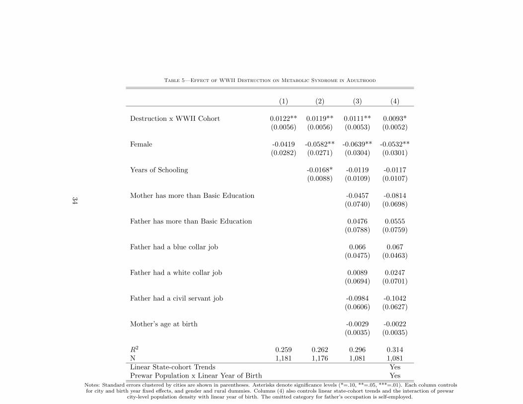
Table 5—Effect of WWII Destruction on Metabolic Syndrome in Adulthood

(1) (2) (3) (4)

Destruction x WWII Cohort 0.0122** 0.0119** 0.0111** 0.0093*(0.0056) (0.0056) (0.0053) (0.0052)

Female -0.0419 -0.0582** -0.0639** -0.0532**(0.0282) (0.0271) (0.0304) (0.0301)

Years of Schooling -0.0168* -0.0119 -0.0117(0.0088) (0.0109) (0.0107)

Mother has more than Basic Education -0.0457 -0.0814(0.0740) (0.0698)



Father had a white collar job 0.0089 0.0247(0.0694) (0.0701)

Father had a civil servant job -0.0984 -0.1042(0.0606) (0.0627)





34

Table 6—Falsification Tests

Body Mass Index Obesity Metabolic Syndrome

(1) (2) (3) (4) (5) (6)

Destruction x Born btw. 1922-1933 -0.0327 0.0068 -0.0042 -0.0008 0.001 -0.0085

(0.0388) (0.0531) (0.0039) (0.0050) (0.0109) (0.0163)

Female -1.2445*** -1.2263*** -0.1287*** -0.1191*** -0.0848 -0.068

(0.2472) (0.2887) (0.0295) (0.0372) (0.0628) (0.0651)

Years of Schooling -0.1459 -0.0118 -0.0194

(0.0893) (0.0092) (0.0191)

Mother has more than Basic Education 0.0086 -0.0031 -0.0167

(0.7047) (0.0876) (0.0844)

Father has more than Basic Education 0.5729 0.0412 0.0557

(0.6344) (0.0772) (0.0814)

Father had a blue collar job 0.1062 0.0133 0.1738

(0.3163) (0.0393) (0.1043)

Father had a white collar job -0.6952 -0.0969** 0.0503(0.4275) (0.0474) (0.1253)

Father had a civil servant job 0.3233 -0.0039 -0.0125(0.6019) (0.0577) (0.1075)

Mother’s age at birth -0.003 0.0001 0.0006(0.0219) (0.0027) (0.0059)

R2 0.134 0.147 0.104 0.125 0.365 0.424N 1312 1216 1312 1216 660 610

Linear State-specific Trends Yes Yes YesPrewar Population x Linear Year of Birth Yes Yes Yes

Notes: Standard errors clustered by cities are shown in parentheses. Asterisks denote significance levels (*=.10, **=.05, ***=.01). The control group isindividuals born between 1951 and 1960. The ”Placebo” affected group is individuals born between 1922 and 1933. Each column controls for city and

birth year fixed effects and gender and rural dummies. The omitted category for father’s occupation is self-employed.

35

Table 7—Validity Checks

Mortality Cohort Mother’s Age Parental Father Father Father died MoveSize at Birth Educ. BC WC during WWII

(1) (2) (3) (4) (5) (6) (7) (8)

Destruction X WWII Cohort -0.003 0.0374 -0.0103 -0.0020 -0.0016 -0.0013 -0.0013 0.0037(0.0018) (0.0469) (0.0425) (0.0019) (0.0021) (0.0015) (0.0019) (0.0025)

Female -0.0821*** -0.0322 0.235 0.0345*** -0.0306** 0.0254*** -0.0129 0.0595***(0.0118) (0.0561) (0.1917) (0.0120) (0.0145) (0.0092) (0.0090) (0.0152)

Years of Schooling -0.0067*** -0.007 0.1970*** 0.0683*** -0.0439*** 0.0242*** 0.0000 0.0303***(0.0024) (0.0142) (0.0496) (0.0037) (0.0033) (0.0025) (0.0024) (0.0043)

R2 0.161 0.548 0.061 0.228 0.1 0.092 0.071 0.116N 4,545 4,545 4,106 4,545 4,545 4,545 4,528 4,528

Note: Notes: Standard errors clustered by cities are shown in parentheses. Asterisks denote significance levels (*=.10, **=.05, ***=.01). Each columncontrols for city and year of birth fixed effects and gender and rural dummies.

36

Table 8—Potential Mechanisms and Heterogeneity in the Effect of WWII Destruction on BMI in Adulthood

Base Female Male Urban Mother Basic Father Basic Father ParentResults Only Only Only Educ Educ fought died

(1) (2) (3) (4) (5) (6) (7) (8)

Destruction X WWII Cohort 0.0777** 0.0939* 0.0567 0.1082* 0.0928** 0.0770* 0.0810** 0.0786**(0.0355) (0.0518) (0.0373) (0.0559) (0.0398) (0.0397) (0.0352) (0.0357)

Years of Schooling -0.2055*** -0.2966*** -0.1355** -0.1711*** -0.1995*** -0.1980*** -0.2086*** -0.2066***(0.0518) (0.0868) (0.0529) (0.0627) (0.0603) (0.0651) (0.0516) (0.0518)

Father fought in WWII -0.2898(0.7114)

Mother died during WWII -0.7290(1.0414)

Father died during WWII -0.2315(0.3612)

R2 0.106 0.160 0.135 0.141 0.118 0.138 0.106 0.106N 2,109 1,122 987 1,200 1,780 1,656 2,104 2,109

Notes: Standard errors clustered by cities are shown in parentheses. Asterisks denote significance levels (*=.10, **=.05, ***=.01). Each column controlsfor city and year of birth fixed effects. Other controls are gender and rural dummies.

37

Table 9—Potential Mechanisms and Heterogeneity in the Effect of WWII Destruction on Obesity in Adulthood

Baseline Female Male Urban Mother Basic Father Basic Father fought Parent diedResults Only Only Only Educ Educ in WWII during WWII

(1) (2) (3) (4) (5) (6) (7) (8)

Destruction X WWII Cohort 0.0077** 0.0096* 0.0041 0.0101* 0.0103** 0.0100** 0.0081** 0.0078**(0.0036) (0.0051) (0.0053) (0.0055) (0.0043) (0.0042) (0.0036) (0.0035)

Years of Schooling -0.0207*** -0.0257*** -0.0187*** -0.0164** -0.0195** -0.0212*** -0.0207*** -0.0209***(0.0058) (0.0088) (0.0065) (0.0064) (0.0075) (0.0078) (0.0058) (0.0058)

Father fought in WWII 0.0287(0.0832)

Mother died during WWII -0.0537(0.1125)

Father died during WWII -0.0701(0.0480)

R2 0.094 0.143 0.130 0.113 0.104 0.130 0.094 0.095N 2,109 1,122 987 1,200 1,780 1,656 2,104 2,109


38

Table 10—Potential Mechanisms and Heterogeneity in the Effect of WWII Destruction on the Metabolic Syndrome in Adulthood

Baseline Female Male Urban Mother Basic Father Basic Father fought Parent diedResults Only Only Only Educ Educ in WWII during war

(1) (2) (3) (4) (5) (6) (7) (8)

Destruction X WWII Cohort 0.0119** 0.0048 0.0197* 0.0212*** 0.0127** 0.0138** 0.0121** 0.0114**(0.0056) (0.0071) (0.0103) (0.0070) (0.0060) (0.0063) (0.0056) (0.0056)

Years of Schooling -0.0168* -0.0287*** -0.0103 -0.0227* -0.0087 -0.0108 -0.0161* -0.0160*(0.0088) (0.0105) (0.0125) (0.0117) (0.0106) (0.0111) (0.0091) (0.0089)

Father fought in WWII 0.1657(0.1236)

Mother died during WWII 0.1645(0.1729)

Father died during WWII 0.0871(0.0754)

R2 0.262 0.352 0.331 0.337 0.286 0.298 0.266 0.264N 1,176 631 545 666 981 925 1,172 1,176


39

Table A-1—Specification with Length of Exposure

Body Mass Index Obesity Health Conditions(1) (2) (3) (4) (5) (6)

Destruction x Number of Years Exposed 0.0262*** 0.0237*** 0.0026*** 0.0027*** 0.0026** 0.0025**(0.0079) (0.0066) (0.0008) (0.0007) (0.0013) (0.0012)

Female -0.9976*** -1.1525*** -0.1245*** -0.1421*** -0.0437 -0.0539*(0.1939) (0.2330) (0.0240) (0.0317) (0.0282) (0.0295)

Years of Schooling -0.1912*** -0.0188*** -0.0115(0.0654) (0.0068) (0.0108))

Mother has more than 0.1292 -0.0052 -0.11Basic Education (0.5469) (0.0583) (0.0732))

Father has more than 0.091 0.0169 0.0696Basic Education (0.5059) (0.0526) (0.0717)

Father had a blue collar job 0.1667 0.0353 0.0702(0.2780) (0.0326) (0.0455)

Father had a white collar job -0.3541 -0.0236 0.0328(0.3092) (0.0343) (0.0710)

Father had a civil servant job 0.513 0.0697 -0.0998(0.4273) (0.0461) (0.0629)

Mother’s age at birth -0.0182 -0.0018 -0.0023(0.0196) (0.0025) (0.0035)

R2 0.097 0.122 0.088 0.115 0.259 0.314N 2,119 1,952 2119 1,952 1,181 1,081Linear State-specific Trends Yes Yes YesPrewar Population x Linear Year of Birth Yes Yes Yes

Notes: Standard errors clustered by cities are shown in parentheses. Asterisks denote significance levels (*=.10, **=.05, ***=.01). Each column is froma separate regression which controls for city and birth year fixed effects, and gender and rural dummies.

40

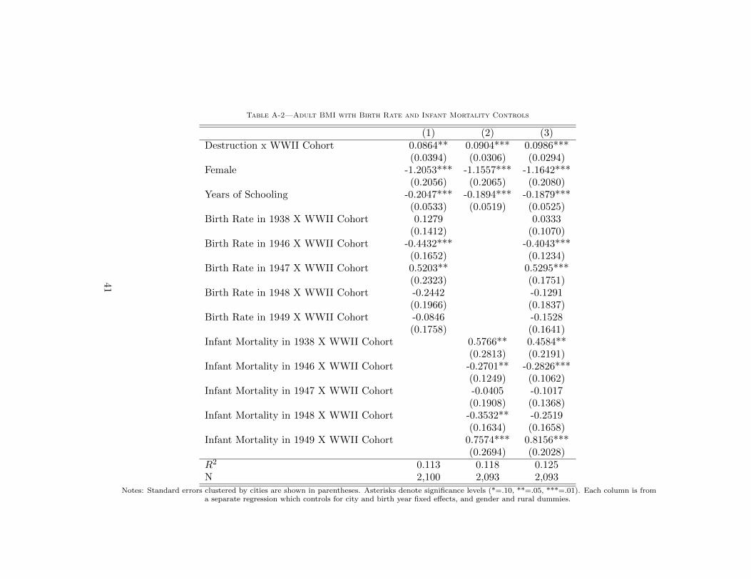
Table A-2—Adult BMI with Birth Rate and Infant Mortality Controls

(1) (2) (3)Destruction x WWII Cohort 0.0864** 0.0904*** 0.0986***

(0.0394) (0.0306) (0.0294)Female -1.2053*** -1.1557*** -1.1642***

(0.2056) (0.2065) (0.2080)Years of Schooling -0.2047*** -0.1894*** -0.1879***

(0.0533) (0.0519) (0.0525)Birth Rate in 1938 X WWII Cohort 0.1279 0.0333

(0.1412) (0.1070)Birth Rate in 1946 X WWII Cohort -0.4432*** -0.4043***

(0.1652) (0.1234)Birth Rate in 1947 X WWII Cohort 0.5203** 0.5295***

(0.2323) (0.1751)Birth Rate in 1948 X WWII Cohort -0.2442 -0.1291


(0.1758) (0.1641)Infant Mortality in 1938 X WWII Cohort 0.5766** 0.4584**

(0.2813) (0.2191)Infant Mortality in 1946 X WWII Cohort -0.2701** -0.2826***

(0.1249) (0.1062)Infant Mortality in 1947 X WWII Cohort -0.0405 -0.1017

(0.1908) (0.1368)Infant Mortality in 1948 X WWII Cohort -0.3532** -0.2519

(0.1634) (0.1658)Infant Mortality in 1949 X WWII Cohort 0.7574*** 0.8156***

(0.2694) (0.2028)R2 0.113 0.118 0.125N 2,100 2,093 2,093


41

Table A-3—Obesity with Birth Rate and Infant Mortality Controls

(1) (2) (3)Destruction x WWII Cohort 0.0084** 0.0082** 0.0086**

(0.0042) (0.0035) (0.0038)Female -0.1458*** -0.1418*** -0.1424***

(0.0259) (0.0258) (0.0260)Years of Schooling -0.0207*** -0.0192*** -0.0192***



(0.0203) (0.0171)Birth Rate in 1947 X WWII Cohort 0.0342 0.0323*



(0.0209) (0.0214)Infant Mortality in 1938 X WWII Cohort 0.0315 0.0250



(0.0194) (0.0171)Infant Mortality in 1948 X WWII Cohort -0.0439** -0.0405*

(0.0192) (0.0222)Infant Mortality in 1949 X WWII Cohort 0.0658** 0.0671***

(0.0281) (0.0241)R2 0.093 0.095 0.097N 2,100 2,093 2,093


42

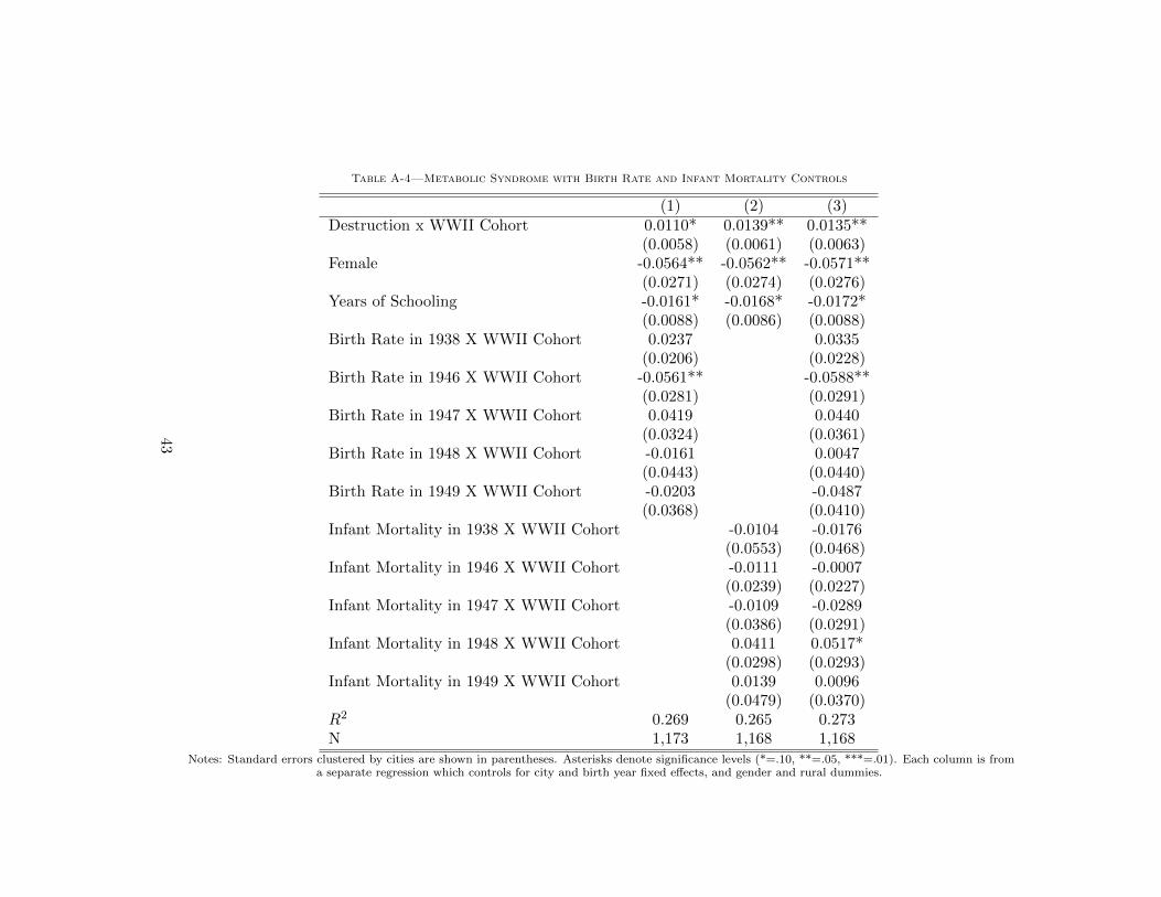
Table A-4—Metabolic Syndrome with Birth Rate and Infant Mortality Controls

(1) (2) (3)Destruction x WWII Cohort 0.0110* 0.0139** 0.0135**

(0.0058) (0.0061) (0.0063)Female -0.0564** -0.0562** -0.0571**

(0.0271) (0.0274) (0.0276)Years of Schooling -0.0161* -0.0168* -0.0172*


(0.0206) (0.0228)Birth Rate in 1946 X WWII Cohort -0.0561** -0.0588**

(0.0281) (0.0291)Birth Rate in 1947 X WWII Cohort 0.0419 0.0440

(0.0324) (0.0361)Birth Rate in 1948 X WWII Cohort -0.0161 0.0047





(0.0386) (0.0291)Infant Mortality in 1948 X WWII Cohort 0.0411 0.0517*


(0.0479) (0.0370)R2 0.269 0.265 0.273N 1,173 1,168 1,168


43

Figure 1. Share of Dwellings Destroyed in German Cities during WWII

Source: Knopp (2001). The size of the circle shows the city size in 1939, where the largest circle refersto cities with more than 500,000 inhabitants; middle-size circle, cities with between 100,000 and

500,000 inhabitants and smallest circle, cities with less than 100,000 inhabitants. The shaded area inthese circles is the share of the dwellings destroyed in the city by the end of WWII.44

Figure 2. Per Capita Postwar City-Level Health Expenditure

Source: Various years of German Municipalities Statistical Yearbook.

45

Figure 3. Destruction of Hospitals and Wartime Destruction

-20

020

40

60

Destr

uctio

n o

f H

ospitals

0 10 20 30City-level Rubble per Capita

95% CI Fitted values

Destruction of Hospitals and Wartime Destruction

Source: The 1939 and 1949 German Municipalities Statistical Yearbook.

46

DIIN PAP SI - IZA Institute of Labor Economicsftp.iza.org/dp10807.pdf · Courtney Ward, Mutlu...

Documents

Transcript of DIIN PAP SI - IZA Institute of Labor Economicsftp.iza.org/dp10807.pdf · Courtney Ward, Mutlu...