Digital Wideband Small Antenna Systemsarlassociates.net/merenda.pdf · Prologue This report is a...
50
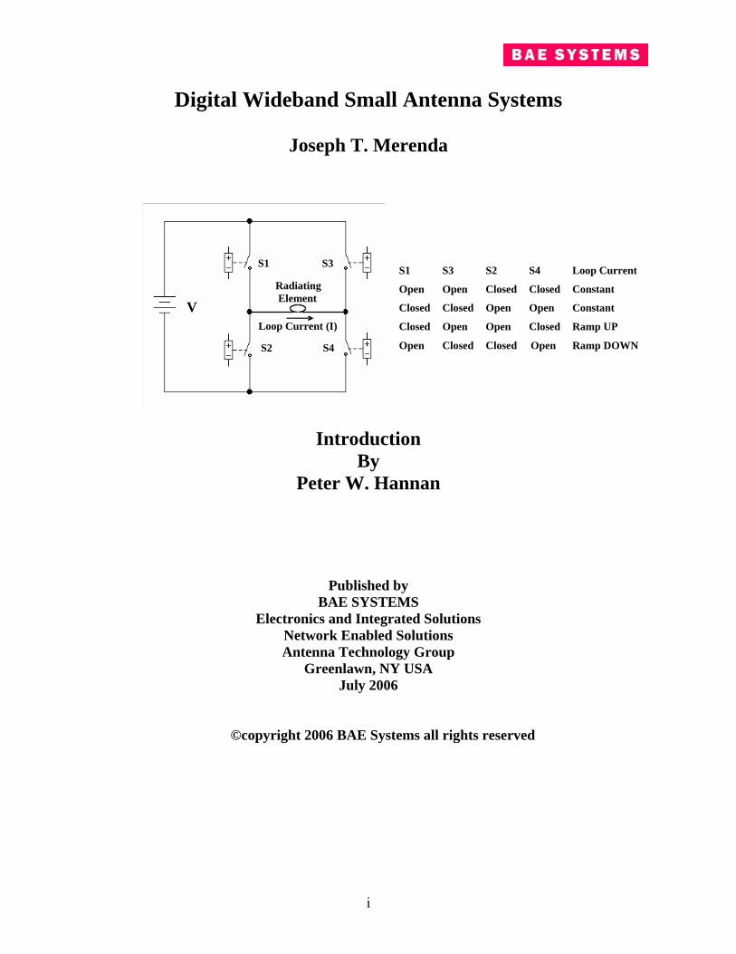
Digital Wideband Small Antenna Systems Joseph T. Merenda S1 S3 S2 S4 Loop Current (I) V Radiating Element S1 S3 S2 S4 Loop Current Open Open Closed Closed Constant Closed Closed Open Open Constant Closed Open Open Closed Ramp UP Open Closed Closed Open Ramp DOWN Introduction By Peter W. Hannan Published by BAE SYSTEMS Electronics and Integrated Solutions Network Enabled Solutions Antenna Technology Group Greenlawn, NY USA July 2006 ©copyright 2006 BAE Systems all rights reserved i
Transcript of Digital Wideband Small Antenna Systemsarlassociates.net/merenda.pdf · Prologue This report is a...
Digital Wideband Small Antenna Systems
Joseph T. Merenda
S1 S3
S2 S4
Loop Current (I)
V Radiating Element
S1 S3 S2 S4 Loop Current
Open Open Closed Closed Constant
Closed Closed Open Open Constant
Closed Open Open Closed Ramp UP
Open Closed Closed Open Ramp DOWN
Introduction By
Peter W. Hannan
Published by BAE SYSTEMS
Electronics and Integrated Solutions Network Enabled Solutions Antenna Technology Group
Greenlawn, NY USA July 2006
©copyright 2006 BAE Systems all rights reserved
i

Prologue This report is a collection of two papers written by Joseph T. Merenda and an introductory paper written by Peter W. Hannan. The Merenda papers introduce a radically new antenna system concept. We have found that some antenna experts have had great difficulty grasping this new idea. An introductory paper has been prepared by Mr. Hannan, which helps in the understanding of the Merenda antenna system. These three papers comprise this report This collection has been given the title “Digital Wideband Small Antenna Systems.” The essence of the basic Merenda antenna system is a set of four switches that connect a battery to an electrically-small loop radiator. T he switches can excite the current on the loop with one of three waveforms: 1) linear increase with time, 2) constant with time, or 3) linear decrease with time. These switches are controlled by a digital processor that converts an input desired radiated waveform into a set of stepped switch commands that produce a loop current with a piecewise linear approximation of the desired radiated waveform. In theory, ideal switches (zero switching time and zero loss) can provide very wideband frequency operation and high system efficiency. In practice, current state-of-the-art switches limit the major efficiency benefits of the wideband Merenda antenna system to frequencies in and below the VHF band. Fortunately, that is where the need is greatest for electrically small antenna systems with enhanced wideband efficiency. In Section 2, Mr. Merenda presents a complete theory of operation and a detailed discussion of the limitations of the new antenna system. He also describes a novel approach for reducing the spectrum-splash problem that is associated with most digital systems. This problem is especially severe for electrically small antennas, which have increasing radiation with increasing frequency. Section 3 reviews the conventional approaches for wideband operation of electrically small antennas. Impedance matching is fundamental for conventional antenna systems. Mr. Merenda describes the “magnitude-matched” design, which is an optimum method for achieving conventional wideband operation for electrically small antennas in a conventional system. The Merenda antenna system is truly a digital antenna system because the process of converting prime (battery) power into radiated power is completely digitized. One final comment: The reader should be prepared to abandon the common notion of impedance matching to be able to appreciate the Merenda antenna system. Henry L. Bachman IEEE Life Fellow IEEE Past President BAE System, NES, Vice President, Retired
Alfred R. Lopez IEEE Life Fellow BAE Systems, NES, Hazeltine Fellow, BAE Systems E&IS Engineering Fellow
ii

For more information contact: John Pedersen or BAE Systems Network Enabled Solutions 450 Pulaski Road Greenlawn, NY 11740-1606 USA Phone: 631.262.8092 Fax: 631.262.8053 Email: [email protected]
Richard Kumpfbeck BAE Systems Network Enabled Solutions 450 Pulaski Road Greenlawn, NY 11740-1606 USA Phone: 631.262.8073 Fax: 631.262.8053 Email: [email protected]
iii

Table of Contents Section 1
An Introductory Note to Readers of the Merenda Papers Peter W. Hannan IEEE Life Fellow BAE Systems, NES, Hazeltine Fellow, Senior Principal Engineer II BAE Systems E&IS Engineering Fellow
Section 2
A Waveform Synthesis Method for Increasing the Efficiency of Electrically Small Transmitting Antenna Systems when Operating over Multi-Octave Bandwidths Joseph T. Merenda BAE Systems, NES, Senior Principal Engineer II
Section 3
Limitations on the Efficiency of Conventional Electrically Small Antenna Systems when Operating over Multi-Octave Bandwidths Joseph T. Merenda BAE Systems, NES, Senior Principal Engineer II
iv
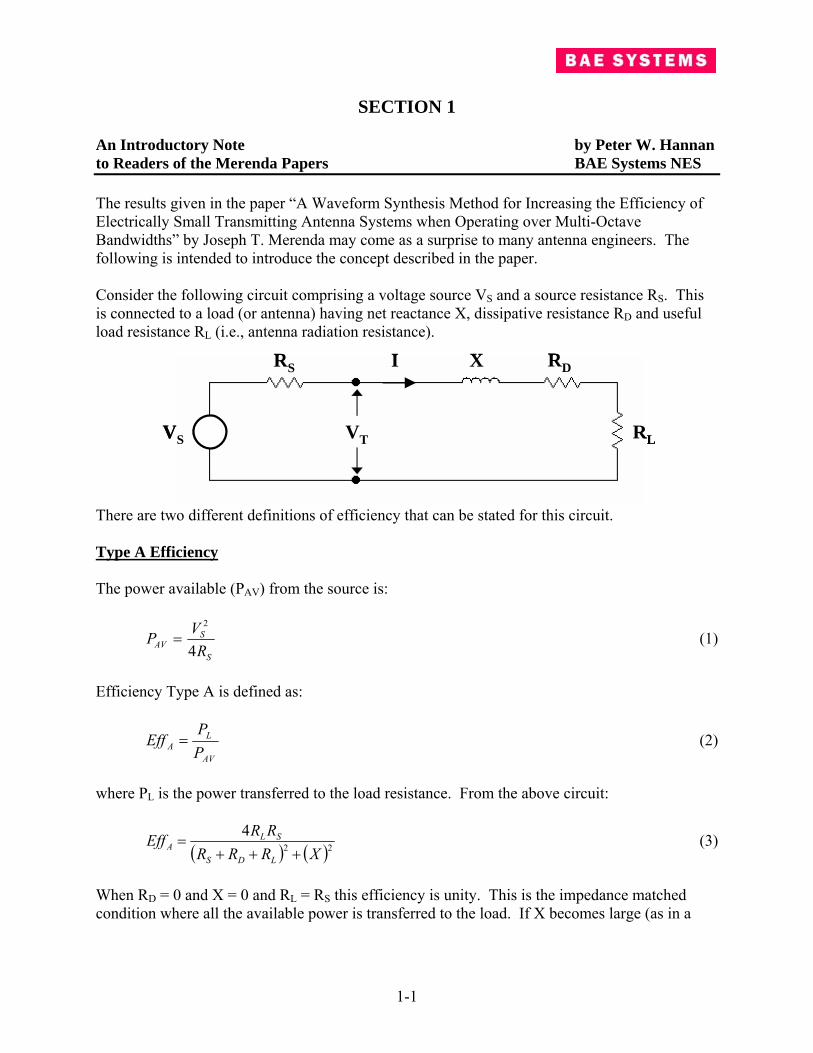
SECTION 1 An Introductory Note by Peter W. Hannan to Readers of the Merenda Papers BAE Systems NES The results given in the paper “A Waveform Synthesis Method for Increasing the Efficiency of Electrically Small Transmitting Antenna Systems when Operating over Multi-Octave Bandwidths” by Joseph T. Merenda may come as a surprise to many antenna engineers. The following is intended to introduce the concept described in the paper. Consider the following circuit comprising a voltage source VS and a source resistance RS. This is connected to a load (or antenna) having net reactance X, dissipative resistance RD and useful load resistance RL (i.e., antenna radiation resistance). RS X RD
RLVTVS
IRS X RD
RLVTVS
I There are two different definitions of efficiency that can be stated for this circuit. Type A Efficiency The power available (PAV) from the source is:
S
SAV R
VP4
2
= (1)
Efficiency Type A is defined as:
AV
LA P
PEff = (2)
where PL is the power transferred to the load resistance. From the above circuit:
( ) ( )22
4XRRR
RREffLDS
SLA +++= (3)
When RD = 0 and X = 0 and RL = RS this efficiency is unity. This is the impedance matched condition where all the available power is transferred to the load. If X becomes large (as in a
1-1

high-Q antenna operated off its resonant frequency), the impedance is poorly matched and this efficiency decreases. Type B Efficiency The power actually delivered (PDEL) by the voltage source is: (4) IVP SDEL •= where I is the source current and • denotes a scalar product. Efficiency Type B is defined as:
DEL
LB P
PEff = (5)
From the circuit:
DSL
LB RRR
REff++
= (6)
When RD = 0 and RS approaches 0, this efficiency approaches unity. Note that this efficiency is independent of the reactance X. Being independent of X suggests that this efficiency might not decrease even with wideband operation of a high-Q untuned antenna. A variation of EffB can be stated in which we are interested only in the efficiency of the load, and we choose to ignore losses in the generator. In this case, the power delivered to the load ( DELP′ ) by the combination of voltage source and source resistance is: (7) IVP TDEL •=′ where VT is the voltage at the terminals of the load. The corresponding efficiency is:
DL
LB RR
RfEf+
=′ (8)
Note again that this efficiency is independent of the reactance X... An alternate description of is: BfEf ′
DL
LB PP
PfEf
+=′ (9)
where PL is the useful power transferred to the load resistance RL and PD is the power lost in the dissipative resistance RD.
1-2

Choice of the Appropriate Type of Efficiency In a transmitting antenna system there is often a power amplifier feeding the antenna. Typical amplifiers operate satisfactorily only when feeding a load that is reasonably well-matched in impedance. This also allows most of the power that is available from the amplifier to be transferred to the load, so the “size” of the amplifier need be no greater than necessary to supply the desired power. Power reflected back toward the amplifier from an imperfectly matched load represents wasted power. The Type A efficiency is the appropriate one to use in this case. The source resistance RS of a typical amplifier is not a physical resistor; rather, it depends on the amplifier characteristics. The value of RS can be determined by finding the load resistance that yields maximum power transfer from the amplifier to the load. Usually the amplifier is designed so that RS is equal to approximately 50 ohms. The large amount of power that is apparently dissipated in RS under matched conditions has no significance and is not included in the determination of EffA. It is important to recognize, however, that EffA is only part of the story. The amplifier itself has an efficiency that is usually far below unity even when operating into a matched load. Other necessary components in the system may also contribute losses. The net antenna/amplifier system efficiency is the product of EffA and amplifier efficiency and the other component efficiencies. Consider now a very different case: a battery-powered flashlight. RS is the internal resistance of the battery and RL is the resistance of the filament in the light bulb. The internal resistance RS is a real resistance that dissipates real power when current flows through the battery. Suppose the objective is to get light for as long as possible from the flashlight. Then we want to maximize EffB by making RL much greater than RS. This will minimize the power wasted in the battery internal resistance and maintain battery voltage across the bulb filament. If, instead, we tried to maximize EffA half the battery power would be wasted. Impedance matching the load to the source is not a good way to operate a flashlight. Consider another example: a 60 Hz, 120V alternator connected to a load. RS is the internal resistance of the alternator and RL is the useful load resistance. Here again we want to maximize EffB and maintain voltage on the load by making RS much smaller than RL. We do not care whether EffA is low, nor that the impedance is poorly matched. We can even get along with high reactance in the load if the alternator can provide the voltage needed to force the desired current through the load reactance. If we get our 60 Hz power from the power company, then we do not worry about the power lost in RS. We only worry about the efficiency of our 60 Hz appliance. In this case, is the quantity that concerns us.
BfEf ′
Suppose we had an alternator that operated at, say, 50 MHz, and suppose the alternator could be varied in speed and voltage to provide FM and AM having substantial modulation bandwidth. Then connecting the alternator directly to an untuned electrically-small reactive antenna might
1-3

provide a product of bandwidth x EffB that exceeds the product that is available with conventional approaches. Such an alternator in the form of a rotating machine is impractical. However, Mr. Merenda has devised practical circuits that provide this function. Mr. Merenda’s Problem The problem that benefited from Merenda’s new approach was the following. An electrically-small loop antenna was to be fed by a VHF transmitter requiring wide modulation bandwidth. The system was to be portable and operated on a battery. High system efficiency was needed in order to avoid premature battery rundown. Investigation of a conventional transmitter using an amplifier feeding a small loop showed that all of the conventional approaches for widebanding the system gave a very low value for EffA. The resulting net system efficiency was so low that battery charge would be rapidly depleted. Merenda’s solution to the problem was to eliminate the amplifier system and replace it with a system that applies battery voltage directly to the loop antenna with alternating polarity so as to yield the desired modulated VHF signal. In this case, EffB (not EffA) is the appropriate factor to evaluate. Actually, in his paper on the waveform synthesis method, Merenda uses because the inclusion of battery resistance loss would be of little interest to the reader and would obscure the comparison with conventional approaches.
BfEf ′
In Conclusion The conventional system in which a transmitting antenna is fed from an amplifier cannot achieve high efficiency when the antenna reactance is large. This results in a severe limit on efficiency when the antenna Q is high and the signal bandwidth is large. An interesting and comprehensive discussion of this limit for the case of multi-octave bandwidths and electrically-small antennas is given in Mr. Merenda's companion paper "Limitations on the Efficiency of Conventional Electrically-Small Antenna Systems when Operating over Multi-Octave Bandwidths". In an antenna system that avoids use of an amplifier, the efficiency (EffB) would be independent of the antenna reactance if the simple series circuit shown on Page 1 accurately represented the system. In practice, the alternating polarity circuits devised by Mr. Merenda have dissipative losses that correspond to resistors in series and in parallel with the antenna. The latter causes the efficiency to be reduced by the antenna reactance. Additionally, the radiated signal contains some harmonics that represent wasted power. Mr. Merenda has analyzed these factors in his paper on the waveform synthesis approach, and has shown that his new antenna system can provide multi-octave bandwidth with a high-Q electrically-small antenna yielding significantly higher efficiency than the conventional antenna system.
1-4

SECTION 2
A Waveform Synthesis Method for Increasing the Efficiency of Electrically Small Transmitting Antenna Systems when
Operating over Multi-Octave Bandwidths
Joseph T. Merenda BAE Systems NES
Greenlawn, NY
ABSTRACT:
A radiating system is described in which electronic switches are embedded in the radiating structure. The switches operate at a rate significantly higher than the RF carrier frequency and are used to digitally synthesize the radiating current waveform. The operating bandwidth is not limited by antenna size. The efficiency of this approach is determined by switch characteristics and the synthesis algorithm. The digital synthesis of radiating current results in spurious radiation at harmonic frequencies. The impact of spurious radiation is mitigated by a unique synthesis algorithm. This non-linear method offers significant efficiency improvement compared to a conventional system using an amplifier and a passive electrically small antenna of the same size when operating over a multi-octave bandwidth. Two prototype small antenna systems are described that operate over instantaneous bands covering 40 to 80 MHz and 30 to 100 MHz, respectively.
I INTRODUCTION Conventional wisdom has long held that electrically small antennas are either inefficient or narrowband. High efficiency and wide bandwidth are incompatible. Modern systems generally exploit large operating bandwidth for a variety of reasons. Hence, the efficiency of an electrically small antenna is usually unacceptably low. Unfortunately, that conventional wisdom has restricted system designers’ options and eliminated the use of lower operating frequencies in some applications because antennas that offer acceptable radiation efficiency are physically too large. For example, propagation properties for ground-to-ground communication systems are superior at lower frequencies. However, in many systems, the lower frequencies are not used because the antennas are very large. In some instances it is possible to deploy a large antenna. However, there is always an advantage in terms of cost, visual properties, and logistical considerations if a smaller antenna could perform equally well.
2-1

The conventional wisdom is not wrong, but it is restricted to passive antenna systems that use lumped tuning components or their distributed counterparts to match the antenna impedance to the generator. One method has been described for increasing the bandwidth or efficiency of electrically small antennas. It uses a variation of the impedance-matching technique by deploying non-Foster reactances (negative capacitors or inductors) to match the antenna. The non-Foster reactances can be realized in theory by proper connections of gain blocks and conventional reactances with feedback. The use of negative reactances enables wideband impedance match and a very high efficiency-bandwidth product. That approach offers the potential for improved performance for receive applications. It appears to be impractical at this time for high power transmit antennas which present the more difficult design challenge when using small antennas. The approach to be described in this paper is specifically for the transmit application. The approach described in this paper deviates from the linear impedance matching concept. There is no port that defines the RF boundary between the antenna and other components in the radio system. No power amplifier is used in this system. The radiating currents are synthesized using a non-linear switching network embedded in the radiating structure and, in its simplest implementation, the only antenna interfaces are to a DC prime power source and a computer that defines the desired current wave shape. Because this system is non-linear and does not use an amplifier, it is not constrained by the limitations imposed on a linear system that requires impedance matching. Hence, it is possible to achieve superior performance. A byproduct of digital synthesis is the generation of undesired frequency components that differ from the commanded wave shape. That is an inherent property of all non-linear systems. A method will be described for mitigation of the impact of undesired radiation frequency components. This paper discusses the limitations on efficiency and bandwidth for the non-linear system when the antenna geometry is electrically small. In theory, it appears possible to achieve high efficiency and very wide bandwidth using this approach, although real non-linear switching component characteristics severely limit that performance. It is important to reiterate that the performance of this system does not violate some basic physical law. The traditional limitations on small antennas are based on the use of passive tuning and linear circuit impedance matching techniques. The performance given for the new antenna system does not violate any portion of that traditional theory, since it ventures outside the realm of traditional assumptions. The limitations on performance when integrating non-linear components has never been explicitly defined in the previous literature. Section II briefly reviews the small antenna problem. Section III describes the basic approach to efficient synthesis of wide band current wave shapes in the radiating structure. Section IV describes one method for generating wide band radiation and the radiation properties of that antenna system. Section V discusses the theoretical efficiency of the non-linear approach. The
2-2
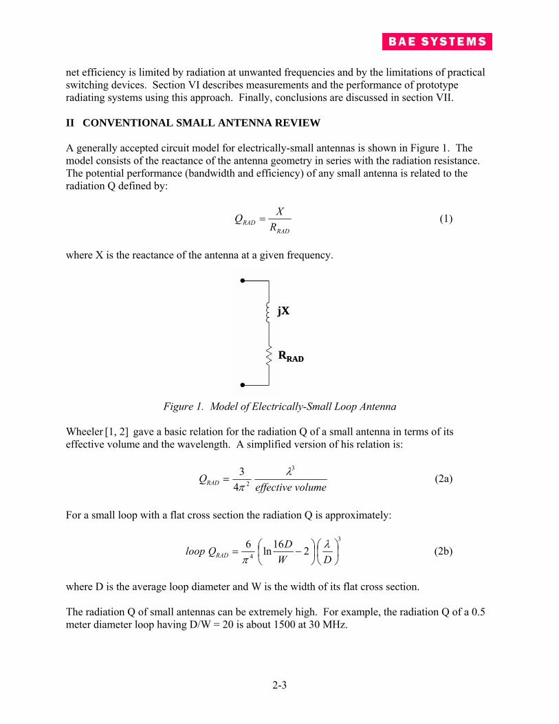
net efficiency is limited by radiation at unwanted frequencies and by the limitations of practical switching devices. Section VI describes measurements and the performance of prototype radiating systems using this approach. Finally, conclusions are discussed in section VII. II CONVENTIONAL SMALL ANTENNA REVIEW A generally accepted circuit model for electrically-small antennas is shown in Figure 1. The model consists of the reactance of the antenna geometry in series with the radiation resistance. The potential performance (bandwidth and efficiency) of any small antenna is related to the radiation Q defined by:
RAD
RAD RXQ = (1)
where X is the reactance of the antenna at a given frequency.
jX
RRAD
jX
RRAD
Figure 1. Model of Electrically-Small Loop Antenna Wheeler [1, 2] gave a basic relation for the radiation Q of a small antenna in terms of its effective volume and the wavelength. A simplified version of his relation is:
volumeeffective
QRAD
3
243 λπ
= (2a)
For a small loop with a flat cross section the radiation Q is approximately:
3
4 216ln6⎟⎠⎞
⎜⎝⎛
⎟⎠⎞
⎜⎝⎛ −=
DWDQloop RAD
λπ
(2b)
where D is the average loop diameter and W is the width of its flat cross section. The radiation Q of small antennas can be extremely high. For example, the radiation Q of a 0.5 meter diameter loop having D/W = 20 is about 1500 at 30 MHz.
2-3

The small antenna problem is thus reduced to a circuit problem. Basic linear matching theory [3, 4, 5] defines the limitations of bandwidth and efficiency as a function of Q where efficiency is defined as the ratio of power delivered to the radiation resistance compared to that available from a generator. Basic courses in electrical engineering teach the concept that the normalized -3dB bandwidth of a high-Q tuned circuit is approximately equal to 1/Q with 100% peak efficiency, but it is possible to operate over larger bands of frequencies while sacrificing efficiency. In fact, the bandwidth-efficiency product of the optimally tuned circuit is approximately constant over a large range of potential bandwidths. It is apparent that the efficiency of an electrically-small antenna in a conventional linear system that operates over a multi-octave band will be very low because the radiation Q is very high. III THE WAVEFORM SYNTHESIS APPROACH The basic circuit shown in Figure 2 overcomes the limitations of linear matching theory. Although the non-linear switching technique applies to both capacitive or inductive antennas, it is easier to implement the technique using inductive loop antennas and all subsequent discussion will concentrate on the electrically-small loop.
Figure 2. Non-Linear Switch Circuit and Small Loop Antenna
S1 S3 S2 S4 Loop current
Open Open Closed Closed Constant
Closed Closed Open Open Constant
Closed Open Open Closed Ramp UP
Open Closed Closed Open Ramp DOWN
S1 S3
S2 S4
Loop Current
IV
The circuit shown in Figure 2 does not include the radiation resistance. The antenna is modeled by the inductor. It has been assumed that the antenna is electrically small (high Q) with the result that the reactance of the inductor is much larger than the radiation resistance. Therefore, the existence of the small radiation resistance has negligible impact on the current that flows through the antenna. Hence, one can accurately determine the antenna current by using the inductive model. The radiated power is equal to: (3) RADRMSRADIATED RIP 2= where IRMS is the RMS alternating current that flows through the inductor or equivalently, the antenna.
2-4

The general terminal relationship between current and voltage in an inductor defines the process of piecewise linear synthesis of arbitrary wave shapes. The rate of change of current I through an inductor is constant and proportional to the voltage V imposed across its terminals.
LV
dtdI
= (4)
where L is the value of the inductor. A useful property of equation 4 occurs when V is equal to zero. In that case the rate of change of inductor current is equal to zero; or, the current is constant. In the absence of resistive losses current will flow undamped for an indefinite period of time providing the terminal voltage is forced to zero (an ideal short circuit across the inductor). There are four useful switch combinations. The useful combinations are listed in Figure 2. In two of the combinations the battery voltage is connected across the inductor, resulting in a constant rate of change of current. The waveform that results is a linear ramp in current. The polarity of the voltage connected across the inductor is different for the two combinations, resulting in either positive or negative going ramps. There are two possible ways to force zero voltage across the inductor (constant current), as shown. The three possible current segments (ramp up, ramp down, constant) can be used to produce a piecewise linear synthesis of any possible current wave shape. An example is shown in Figure 3. As in any digital synthesis of a waveform, the fidelity of the output depends on the increment duration, or the sampling rate compared to the highest rate of change in the desired wave shape.
Figure 3. Piece-Wise Linear Synthesis of Arbitrary Current Waveform Note that the wave shape is not restricted in any way. That fact implies wide bandwidth, provided a rapid sampling rate is possible. Most RF systems do not require infinite flexibility in the composition of the time waveform. In fact, the shape between zero crossings is generally sinusoidal. Although individual pulses are sinusoidal, the required operating bandwidth is large because the time between zero crossings varies by a large amount. Each of the sinusoidal pulses may be approximated in a piecewise fashion by the trapezoid shown in Figure 4. The trapezoidal approximation to a sinusoid has
2-5
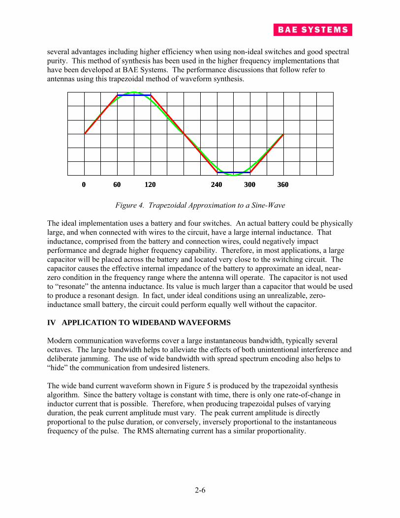
several advantages including higher efficiency when using non-ideal switches and good spectral purity. This method of synthesis has been used in the higher frequency implementations that have been developed at BAE Systems. The performance discussions that follow refer to antennas using this trapezoidal method of waveform synthesis.
0 60 120 240 300 3600 60 120 240 300 360
Figure 4. Trapezoidal Approximation to a Sine-Wave The ideal implementation uses a battery and four switches. An actual battery could be physically large, and when connected with wires to the circuit, have a large internal inductance. That inductance, comprised from the battery and connection wires, could negatively impact performance and degrade higher frequency capability. Therefore, in most applications, a large capacitor will be placed across the battery and located very close to the switching circuit. The capacitor causes the effective internal impedance of the battery to approximate an ideal, near-zero condition in the frequency range where the antenna will operate. The capacitor is not used to “resonate” the antenna inductance. Its value is much larger than a capacitor that would be used to produce a resonant design. In fact, under ideal conditions using an unrealizable, zero-inductance small battery, the circuit could perform equally well without the capacitor. IV APPLICATION TO WIDEBAND WAVEFORMS Modern communication waveforms cover a large instantaneous bandwidth, typically several octaves. The large bandwidth helps to alleviate the effects of both unintentional interference and deliberate jamming. The use of wide bandwidth with spread spectrum encoding also helps to “hide” the communication from undesired listeners. The wide band current waveform shown in Figure 5 is produced by the trapezoidal synthesis algorithm. Since the battery voltage is constant with time, there is only one rate-of-change in inductor current that is possible. Therefore, when producing trapezoidal pulses of varying duration, the peak current amplitude must vary. The peak current amplitude is directly proportional to the pulse duration, or conversely, inversely proportional to the instantaneous frequency of the pulse. The RMS alternating current has a similar proportionality.
2-6

Figure 5. Wide Band Trapezoidal Waveform We now examine the impact on radiated power as a function of frequency. As noted, the electrically small antenna can be modeled as a high-Q circuit. In the case of the loop the equivalent circuit is the geometric inductance in series with the small radiation resistance. The radiation Q is proportional to the cube of wavelength. Therefore, the radiation resistance of a small loop antenna will increase in proportion to the fourth power of frequency. (5) 4ftoalproportionRRAD
The radiated power was defined in equation 3. Since the RMS current varies inversely with frequency when using the trapezoidal method of synthesis, it is then possible to predict the frequency variation of the radiated power. (6) 2ftoalproportionPRAD
In most passive antenna systems one tries to obtain high efficiency across the entire band of operation, leading to the assumption that uniform radiated power versus frequency is a desirable characteristic. However, electrically-small, wide band passive antenna systems tend to exhibit a square-law or cubic frequency variation in efficiency, depending on the exact network configuration. In many cases other factors in the radio link including ground-wave propagation loss and blockage effects increase with frequency. The excess high frequency propagation loss is compensated by greater high frequency radiated power. Hence, radiated power that is proportional to the square of frequency can result in a radio link range that is nearly independent of frequency. In most cases it is more desirable to provide constant link range versus frequency rather than constant radiated power. Therefore, the square-law variation of radiated power versus frequency may actually represent a desirable characteristic. It should be noted that it is possible to produce other current waveforms that result in different radiation vs. frequency characteristics using other synthesis algorithms. The non-linear technique may be used to synthesize piece-wise linear approximations to any waveform. A more complex version of the trapezoidal method offers flexibility in the amplitude of individual trapezoid pulses. The method shown above and discussed in this paper offers the best high-
2-7

frequency performance. A description and performance estimate of other methods may be described in subsequent papers. V CALCULATION OF SYSTEM EFFICIENCY System efficiency is defined in this paper as the ratio of power radiated with the desired waveform compared to the power taken from the battery. There are two main items that prevent one from obtaining 100% efficiency. The first item is the power that is lost in a practical switching system. This is typically the most important item. The second item is the portion of the radiated power that is wasted in spurious spectral content generated by the non-linear switching process. These two items are discussed in this section. A potential additional item, resistive dissipation in the loop itself, is not discussed because it is typically a small loss compared with the switch loss. Loss from Practical Switches There are four factors that contribute to loss in the switching system. Those factors are: switch resistance, switch capacitance, non-zero switching time, and drive energy that is required for switch control. The ideal switches in Figure 2 were replaced with simple switch models in Figure 6. That model includes the parasitic resistance and capacitance of a typical switch. When the switch is closed, it behaves as a small resistor. When current flows through the closed switch some power will be dissipated by the resistance.
S1
S4S2
S3S1
S4S2
S3
Figure 6. Non-Linear Antenna Model Using Real Switches
2-8

When the switch is open, it behaves as a small capacitor. The mechanism for dissipation resulting from the capacitor is less obvious. Prior to switch closure, there is generally some voltage across the switch. The internal capacitance of the switch is charged to that voltage. The charged capacitor stores electrical energy. Subsequently, when the switch closes, the capacitor is discharged by the internal resistance, dissipating the stored energy in that resistor. The power dissipation caused by this effect is proportional to the rate of closure in instances per second. At higher frequencies this effect could actually dominate the total circuit dissipation. The third cause of dissipation is non-zero switching time. The dissipation mechanism is demonstrated in Figure 7. During the transition time the switch simultaneously passes current with a voltage across its terminals. Instantaneous power is defined by the product of the current and the voltage. The average power dissipation caused by the transition effect is related to the percentage of time during the waveform that the switch occupies the transition state. Given that device switching time is relatively constant, it can be seen that this dissipation factor is also proportional to the instantaneous frequency of the synthesized signal.
TS
0
1Current
Voltage
Power
TS
0
1Current
Voltage
Power
Figure 7. Switch Transition Dissipates Power The last factor is the energy required to control and activate the switches. Experience with VHF circuits of this type indicates that an equal amount of power will be dissipated by the drive circuits compared to the sum of the three other mechanisms at the upper frequency limit. This factor decreases at lower operating frequencies. The upper frequency limit is often limited by the capacitor-induced dissipation. A method has been developed when using the trapezoidal synthesis algorithm that eliminates the dissipation caused by the switch capacitor. We call this method the Trapezoidal Staggered Switch (TSS) algorithm. The Algorithm improves the radiation efficiency of the non-linear radiation approach and extends the useful frequency range to upper VHF using switching devices presently available. The upper frequency limit is then limited by the switch transition time. The upper limit (FH) is approximately equal to the frequency where the transition time is about one radian in duration: SH TF π2/1≈ .
2-9

A secondary benefit of the TSS algorithm is a substantial reduction in harmonic radiation, thereby reducing unwanted radiation and improving the desired radiation efficiency. In order to understand the TSS algorithm, let’s examine the switching circuit (Figure 6) as it progresses through a half-sinusoidal pulse (Figure 8). At t = 0 -, the loop current is equal to 0. At t = 0, switches S1 and S4 are closed, and the inductor current ramps up. At t = 1, switch S2 closes while S1 simultaneously opens. The voltage across the inductor is now equal to 0, the loop current remains constant at a value equal to that at t=1-, and the flat-top portion of the trapezoidal approximation to the sinusoidal pulse begins. At this transition time, energy dissipation results from the charged switch capacitance on S2. At t = 1-, the full supply voltage is across S2, while at t=1+, the voltage across S2 will be 0. Therefore, its ON resistance will dissipate all the energy stored in S2’s capacitance.
2
1.5
1
0.50
0
210Time
Inductor Current
Switch Voltage
2
1.5
1
0.50
0
210Time
Inductor Current
Switch Voltage
Figure 8. Switch Waveforms Now, let’s suppose that instead of simultaneously changing the two switch states, we stagger the switching times (Figure 9). At some appropriate time before t=1, open S1. The current continues to flow through the inductor, and begins discharging capacitance of S2 while simultaneously charging the capacitance of S1. As the capacitor charge changes, the voltage across the inductor falls, and the rate at which the inductor current is rising begins to slow down. Finally, at some later time (approx. t = 1.25 in this case), the voltage at the junction of S1 and S2 has fallen to zero and the inductor current has stopped rising. At that time, one can close S2 without dissipating any energy. In addition, the gradual transition in inductor current waveform from a ramp to a constant value more closely approximates the sinusoidal pulse, and results in lower spurious harmonics. A similar staggered switching process can be followed at each of the break points in the trapezoid to eliminate switch capacitance energy dissipation. In all cases, the closed switch is opened before its counterpart is closed, allowing the switch capacitance to discharge before closing its switch.
2-10

2
1.5
1
0.50
0
210Time
Inductor Current
Switch Voltage
2
1.5
1
0.50
0
210Time
Inductor Current
Switch Voltage
2
1.5
1
0.50
0
210Time
Inductor Current
Switch Voltage
Figure 9. Staggered Switching Transient Waveforms
This algorithm was implemented primarily to eliminate the switch dissipation caused by its parasitic capacitance. At high frequencies this form of dissipation predominates over ON state resistive dissipation. A secondary benefit of this approach is that the corner rounding tends to reduce high order harmonics by a large amount. An approximate equation for the total power dissipation of the switching system using this approach is derived in Appendix A. The dissipation depends on the battery voltage and the magnitude of the synthesized current.
⎟⎟⎠
⎞⎜⎜⎝
⎛+⎟
⎟⎠
⎞⎜⎜⎝
⎛+=
HS
D
HPSW,DISS F
ffT
fFFVIP 1
344 2π
(7)
where V is the battery voltage, IP is the peak current, FH is the upper frequency limit of the circuit, f is the operating frequency, and TS is the inherent transition time of the switch.
SH TF π2/1= . FD is a commonly-used figure of merit of the switching devices:
RC
FD1
= (8)
where R is the switch resistance and C is the switch capacitance. The figure of merit for a particular type switch is relatively constant. For example, even though there are many suitable GaAs FETs that are available for switches, with resistance varying from a fraction of an ohm to tens of ohms, the FD of all GaAs FET switches is about 500 GHz. As discussed in Appendix A an optimum antenna reactance exists that enables one to operate up to FH and maximize efficiency at lower frequencies. That optimum reactance depends on the parasitic properties of the switching devices. In most cases it is best to select a switch that is compatible with the antenna rather than attempting to transform the antenna reactance.
2-11

Spectral Analysis The piecewise-linear method of synthesizing the antenna current results in the generation of undesired spectral radiation. That unwanted radiation has the potential for degrading the efficiency because it represents wasted power. However, it will be seen that the wasted power resulting from this effect is far less than the power dissipated in the switching circuit using practical switches. Therefore, the spectral efficiency has little impact on the net efficiency of the system when constructed with switching devices that are presently available. Although the spectral efficiency of other synthesis algorithms is lower than the TSS algorithm, in most systems using those other algorithms it has also been found that the spectral efficiency has little impact on the net efficiency. In the future, the introduction of higher quality switches may allow the spectral efficiency to have a significant impact on the net efficiency. As will be shown, the TSS synthesis algorithm mitigates the spectral loss by a large amount. In addition, the TSS substantially reduces the potential for interfering with other radio systems and greatly enhances the LPI (low probability of intercept) quality of the radiation compared to other synthesis algorithms. Since the switching process is always synchronous with the waveform when using the trapezoidal waveform, only harmonics of the desired instantaneous frequency are generated. If spread spectrum encoding is used to “hide” the radiated signal from undesired listeners, the harmonic radiation will also be spread and hidden. Other synthesis algorithms will exhibit strong spurious radiation at and around the sampling frequency, independent of the instantaneous frequency. The Fourier transform of the trapezoidal approximation to a sine wave exhibits an extremely small amount of spectral distortion when the transition points are chosen at the 60, 120, 240, and 300 degree points in the sine waveform. All the even harmonics along with every third odd harmonic are theoretically equal to zero as shown in Figure 10. The first theoretical harmonic that exhibits signal power is the fifth harmonic and it is 28 dB below the fundamental. For applications other than small antennas, the spurious harmonic performance would be excellent and introduce no major problems. However, the small antenna application is unique in that the radiation resistance increases at higher frequencies. That effect magnifies the higher harmonics and reduces their effective rejection. The radiation at each harmonic is found by: ( ) ( )fR)f(IfP RADRMSRAD
2= (9)
2-12
-120-110-100
-90-80-70-60-50-40-30-20-10
0
1 7 13 19 25 31 37 43 49 55 61 67 73 79 85 91 97
Harmonic Number
Am
plitu
de (d
b)
Figure 10. Spectral Content for Simple Trapezoid (фS = 0) The radiation resistance (RRAD) of a small loop varies as the fourth power of frequency (equation 5). As shown in Figure 11, the resulting harmonic radiation theoretically remains at the same level as the fundamental, assuming that the antenna remains electrically small at all harmonic frequencies. Therefore, the radiated power of higher order harmonics could be very substantial.
-40-35-30-25-20-15-10
-505
1 7 13 19 25 31 37 43 49 55 61 67 73 79 85 91 97
Harmonic Number
Am
plitu
de (d
b)
Figure 11. Harmonic Radiated Power for Simple Trapezoid (фS = 0) The use of the TSS algorithm rounds the corners of the trapezoidal approximation, as shown in Figure 12. фS is the relative time stagger. It is the amount out of the 360-degree sinusoid that the closing switch is delayed after opening its counterpart, as discussed earlier.
2-13

-80-70-60-50-40-30-20-1001020304050607080
0 20 40 60 80 100
120
140
160
180
200
220
240
260
280
300
320
340
360
RelativeTime (degrees)
Am
plitu
de φS = 300
φS = 100
φS = 200
φS = 50
φS = 00
Figure 12. Current Waveform vs. Relative Time Stagger (фS)
The corner rounding significantly reduces the higher order harmonics, as shown in Figure 13. Figure 13 shows the harmonic envelope for each stagger condition. The detailed frequency characteristic of each condition is the same as the фS = 0 condition, i.e., all even and every third harmonic are equal to zero. The radiated power envelopes with various stagger durations are shown in Figure 14.
-120-110-100
-90-80-70-60-50-40-30-20-10
0
1 11 19 29 37 47 55 65 73 83 91
Harmonic Number
Am
plitu
de (d
b)
φS = 00
φS = 100
φS = 50
φS = 150
φS = 200
φS = 250
φS = 300-120-110-100
-90-80-70-60-50-40-30-20-10
0
1 11 19 29 37 47 55 65 73 83 91
Harmonic Number
Am
plitu
de (d
b)
φS = 00
φS = 100
φS = 50
φS = 150
φS = 200
φS = 250
φS = 300
φS = 00
φS = 100
φS = 50
φS = 150
φS = 200
φS = 250
φS = 300
Figure 13. Harmonic Envelope vs. Relative Time Stagger (фS)
2-14

-40-35-30-25-20-15-10
-505
1 11 19 29 37 47 55 65 73 83 91
Harmonic Number
Am
plitu
de (d
b)φS = 00
φS = 100
φS = 50
φS = 150
φS = 200
φS = 250
φS = 300-40-35-30-25-20-15-10
-505
1 11 19 29 37 47 55 65 73 83 91
Harmonic Number
Am
plitu
de (d
b)φS = 00
φS = 100
φS = 50
φS = 150
φS = 200
φS = 250
φS = 300
φS = 00
φS = 100
φS = 50
φS = 150
φS = 200
φS = 250
φS = 300
Figure 14. Radiated Power Envelope vs. Relative Time Stagger (фS)
The spectral efficiency is here defined as the ratio of desired power radiated (fundamental) to the sum of all the power radiated (fundamental plus all harmonics). The following analysis gives approximate values for the spectral efficiency as a function of the significant variables. The radiation resistance variation of the loop has been modeled as proportional to the fourth power of frequency to infinity. This ignores the change that occurs at approximately the frequency where the loop diameter is a half wavelength. Above that frequency the radiation resistance increases approximately proportional to frequency assuming uniform current [6]. This effect can be expected to greatly reduce the power radiated in the harmonics above the half-wave-diameter frequency. In addition, the simple inductive model used to define the time waveform may no longer be valid. In view of the above, the spectral efficiency will be estimated here by including in the power summation only harmonics that lie below the half-wave-diameter frequency. We define the following limited summation for spectral efficiency:
∑=
= j
mm
j
Peffspectral
1
1 (10)
where m is the harmonic number, j is the highest harmonic included, and Pm is the normalized radiated power shown in Figure 14. The resulting spectral efficiency is plotted as a function of j and фs in Figure 15. It is seen that when фs = 0 the spectral efficiency decreases continuously to a low value as j is increased. However, when фs = 25° or 30° the spectral efficiency levels off to a minimum of -4 or -3 dB as j is increased. A plot of spectral efficiency vs. loop size can be derived from Figure 15. For this purpose we limit j to the harmonic corresponding approximately to the half-wave-diameter frequency. For example, a loop 0.005 wavelengths in diameter at the fundamental frequency would require the summation of the first hundred harmonics. The result is shown in Figure 16 with фs as a parameter.
2-15

-16-15-14-13-12-11-10
-9-8-7-6-5-4-3-2-10
1 11 19 29 37 47 55 65 73 83 91
Number of harmonics
Spec
tral E
ffici
ency
(db)
φS = 00
φS = 100
φS = 50
φS = 150
φS = 200
φS = 250
φS = 300
-16-15-14-13-12-11-10
-9-8-7-6-5-4-3-2-10
1 11 19 29 37 47 55 65 73 83 91
Number of harmonics
Spec
tral E
ffici
ency
(db)
φS = 00
φS = 100
φS = 50
φS = 150
φS = 200
φS = 250
φS = 300
φS = 00
φS = 100
φS = 50
φS = 150
φS = 200
φS = 250
φS = 300
Figure 15. Spectral Efficiency vs. Number of Harmonics Included and фS
-16-15-14-13-12-11-10
-9-8-7-6-5-4-3-2-10
0 0.01 0.02 0.03 0.04 0.05 0.06 0.07 0.08 0.09 0.1
Spec
tral E
ffici
ency
(db)
φS = 300
φS = 200
φS = 250
φS = 150
φS = 100
φS = 50
φS = 00
Loop DiameterWavelength
Figure 16. Spectral Efficiency vs. Loop Size and фS It is seen from Figure 16 that the only case where the spectral efficiency continues to degrade as the antenna gets smaller is that of the pure trapezoid. For most values of фS the efficiency settles at some asymptotic value. If фS is greater than 15 degrees, the minimum spectral efficiency is about -6dB, and for фS = 30° the minimum spectral efficiency is about -3dB.
2-16

System Efficiency The net system efficiency may be found by dividing the desired power radiated (PRAD, DES) by the sum of the total power radiated (PRAD, TOT) and the power dissipated in the switching system (PDISS):
DISSTOT,RAD
DES,RAD
PPP
EffSystem+
= (11)
The desired radiation is equal to:
RAD
P
RAD
PPRADRMSDESRAD Q
VIQ
XIIRIP22
2, === (12)
The total radiation is given by:
⎟⎟⎠
⎞⎜⎜⎝
⎛⎟⎟⎠
⎞⎜⎜⎝
⎛= ∑
=
j
mM
RAD
PTOTRAD P
QVIP
1, 2
(13)
The dissipated power is given in equation 7. The system efficiency is then given by:
∑ = ⎟⎟⎠
⎞⎜⎜⎝
⎛+⎟
⎟⎠
⎞⎜⎜⎝
⎛++
=j
mH
SD
HRADM F
ffTfF
FQP
EffSystem
1
2
13442
1π
(14)
Equation 14 is somewhat difficult to evaluate because фS and the number of harmonics in the summation vary with frequency. Therefore, the Fourier terms and the power summation must be evaluated separately for each frequency in the operating band. A simplified example is given in which the efficiency of a particular system is computed from (14) for a 0.5m diameter loop. The assumed switching parameters used are representative of currently available GaAs switches. Three values of spectral efficiency are assumed: 0 dB, -3 dB, and -6 dB. The latter two values are obtainable with Φs = 30° and 15°, respectively (see figure 16). The results are shown in Table 1.
2-17

Table 1. Computed Wideband System Efficiency* SYSTEM EFFICIENCY (dB)
Assumed Spectral Efficiency f (MHz) QRAD 0 dB -3 dB -6 dB 25 3202 -26.2 -26.2 -26.3 50 400 -19.3 -19.3 -19.4 100 50 -13.8 -14.0 -14.3
* loop D = 0.5m FD = 500 GHz loop W = 0.025m FH = 150 MHz TS = 1 ns
It is seen that for this representative example, the harmonics summation term of (14) has a very small effect on the system efficiency except at the highest frequencies where its effect is still rather small. With a smaller size loop the harmonic summation term will have even less effect. The values for system efficiency given in Table 1 are low, but the antenna system operates over at least the 4 to 1 frequency band shown. It will be seen in the next section that the efficiency of this waveform-synthesis system is substantially higher than the efficiency of a representative conventional wideband antenna system having the same size antenna. VI MEASURED RESULTS AND COMPARISON WITH THEORY The predicted performance of the waveform synthesis approach has been verified through the construction of several prototype loop antenna systems ranging in frequency from 20 KHz to 150 MHz. A VLF antenna used a different synthesis algorithm that was capable of generating arbitrary waveform shapes. It may be discussed in a later paper. A very small VHF loop (2.5 inch diameter) verified the equations describing the performance with the TSS algorithm. It will be described here. Other larger VHF antennas have been constructed that radiate a greater and more useful signal level. Those antennas have been successfully demonstrated in VHF radio communication links, and may be described in another paper. The performance of one of the larger VHF antennas is summarized here. Measured Efficiency Ratio with 2.5-Inch Loop The 2.5-inch diameter loop is shown in Figure 17. The loop was printed on the circuit board that contains the switch bridge and drivers. (The gaps seen in the top and bottom of the loop contain large capacitors to block DC without affecting the RF. The right-hand gap contains a low-impedance current-measuring device.) The system efficiency ideally would be measured by measuring the desired radiated power and comparing that to the total power supplied by DC sources. Unfortunately, it is very difficult to accurately measure the radiation of an electrically-small VHF antenna. Therefore, we chose to evaluate the antenna by a comparison measurement.
2-18

Figure 17. Prototype 2.5-inch VHF Loop Antenna System The comparison measurement was performed by comparing both the radiated level and prime power input of this antenna system relative to those of an identical antenna that was fed in a conventional manner. The relative radiation between the two antenna systems is evaluated by placing a probe in proximity with the radiator. The probe is precisely located by a mechanical fixture to insure equal coupling to both antenna types. The prime power input to both antenna systems is easily measured using DC voltage and current meters. For the Figure 17 system this included all the power needed to drive the switches as well as power delivered by the battery to the RF circuit. The Figure 17 antenna system synthesizes the radiating currents from a DC power source. Thus, it replaces the power amplifier in a conventional radiating system. A fair comparison of the system efficiency of the two approaches demands that the DC power required by the amplifier in the conventional approach be included in its total input. A block diagram of the representative wideband conventional antenna system used for the comparison is shown in Figure 18. The power amplifier should be linear in order to supply multi-octave signals. The efficiency of the linear amplifier is estimated at 33% or 1/3. The 3dB attenuator is used to stabilize the input impedance of the antenna in order to present a VSWR less than 3:1 to the amplifier. Greater VSWR tends to reduce the efficiency and increase distortion in the PA. The 2.5-inch diameter loop was selected because its inductive reactance is 50 ohms near the center of the measurement band. It is shown in a companion paper [7] that when the source resistance value matches the midband reactance value of a high-Q antenna, the corresponding efficiency is equal to 2/QRAD, and this remains a good approximation over a wide frequency band. The efficiency ratio of the measured 2.5-inch Figure 17 antenna system relative to the measured conventional Figure 18 system was determined as described above at three discrete frequencies. The results of this direct comparison measurement are shown by the red points in Figure 19.
2-19

PA 3 dbAttenuator
Battery
Small PassiveLoop Antenna
Eff = 1/3 Eff = 1/2 Eff = 2/QRAD
PA 3 dbAttenuator
Battery
Small PassiveLoop Antenna
Eff = 1/3 Eff = 1/2 Eff = 2/QRAD
Figure 18. Block Diagram of Conventional Antenna Radiating System
Theoretical Efficiency Ratio For the conventional system shown in Figure 18 the net DC to radiated power efficiency was derived in [7] and is assumed equal to:
RADQ
EffSystemalConvention3
1= (15)
The theoretical efficiency of the waveform-synthesis system can be compared to that of the conventional system by dividing equation 14 by 15. The result is the efficiency ratio of the two approaches for the same size loop antenna. Equation 16 ignores the small contribution to efficiency degradation caused by spectral content. This approximation allows the efficiency ratio to become independent of radiation Q.
⎟⎟⎠
⎞⎜⎜⎝
⎛+⎟
⎟⎠
⎞⎜⎜⎝
⎛+
≈
H
S
D
H
FffT
fFFEffSystemalConvention
EffSystem
13
8
32π
(16)
This theoretical efficiency ratio is shown over a 20 to 150 MHz band by the blue curve in Figure 19. The parameters are those of the GaAs switches used in the Figure 17 antenna system: TS = 1 ns, FD = 500 GHz, and FH = 150 MHz based on a transition time of about one nanosecond.
2-20

(dB
)C
onve
ntio
nal S
yste
m E
ffSy
stem
Eff
(dB
)C
onve
ntio
nal S
yste
m E
ffSy
stem
Eff
0.002.004.006.008.00
10.0012.0014.0016.00
20 30 40 50 60 70 80 90 100
110
120
130
140
150
Frequency (MHz)
TheoryMeas1Meas2
(dB
)C
onve
ntio
nal S
yste
m E
ffSy
stem
Eff
(dB
)C
onve
ntio
nal S
yste
m E
ffSy
stem
Eff
0.002.004.006.008.00
10.0012.0014.0016.00
20 30 40 50 60 70 80 90 100
110
120
130
140
150
Frequency (MHz)
TheoryMeas1Meas2
0.002.004.006.008.00
10.0012.0014.0016.00
20 30 40 50 60 70 80 90 100
110
120
130
140
150
Frequency (MHz)
TheoryMeas1Meas2
Figure 19. Measured Efficiency Ratio vs. Theory for Two Wideband Systems
Measured Efficiency Ratio with 0.5 Meter Loop Following the encouraging results from this prototype 2.5-inch loop system, a larger, 0.5 meter loop system was developed. This loop is fed from eight switching modules distributed around the loop. The eight feeds provide higher power and maintain uniform current around the larger loop. Figure 20 shows this system in a crossed loop configuration. (The four conductors seen on each loop provide prime power to the switching system but act together as a single turn at RF.) For an efficiency comparison measurement similar to the first one, eight conventional amplifiers would have been needed, but these were not available. Instead, the following procedure was used. The inductance of one of the eight loop sections was calculated and an inductor having that value was connected to one of the eight switch modules. The resulting inductor current was measured at each frequency and the radiated power for a 0.5 meter loop was calculated based on the calculated radiation resistance of the 0.5 meter loop ( ). The input prime power to the switching module was measured; this included all the power needed to drive the switches as well as the power delivered by the battery to the RF circuit. The ratio of radiated power to prime power yielded the system efficiency at each frequency. Comparing this system efficiency with the assumed conventional figure 18 system efficiency of 1/3 Q
RADRMSRAD RIP 2=
RAD yielded the efficiency ratio. Those results are shown by the yellow points from 30 to 100 MHz in figure 19.
2-21

Figure 20. One-Half Meter VHF Crossed Loop Antenna System Details of the 0.5 meter antenna system may be described in a later paper. The switching modules use the same switch design as the 2.5-inch prototype antenna. 32 of the switch modules were constructed and all demonstrated performance extending from 30 to 100 MHz. Comments on Results Inspection of Figure 19 shows good correlation between the theoretical results and the measured results. Both the theory and the measurements demonstrate that the system efficiency of the new waveform-synthesis technique is better than the system efficiency of the representative conventional approach by an average of 10dB in the VHF band. That is a significant factor if one considers battery energy required in many remote and man-portable systems. Of course, a narrow-band conventional small antenna system will achieve higher efficiency than the broad band conventional antenna system used for comparison in this test. The narrow band conventional antenna system may, depending on bandwidth, also exhibit better efficiency than the wideband waveform-synthesis antenna system. However, the waveform-synthesis approach
2-22

offers the advantages of multi-octave frequency coverage and immunity from many local environment effects that tend to detune narrow-band antennas. The waveform-synthesis approach clearly offers superior efficiency over the selected conventional antenna system in a multi-octave application. A companion paper [7] discusses the selected conventional antenna system as well as several other conventional approaches. A key point in that paper is that the efficiency of the conventional antenna system used in this test is representative of what may be achieved in any conventional antenna system when the bandwidth exceeds two octaves. VII CONCLUSIONS Conventional wisdom believes that wide bandwidth and high efficiency are incompatible when using an electrically small antenna. That previous convention is true for passive antennas connected to conventional amplifiers or generators. However, it has been shown here that by combining a non-linear switching network with the antenna to synthesize the desired current waveform, the conventional limitation on bandwidth-efficiency product no longer applies. There is a practical limit on the efficiency of the waveform-synthesis approach because of the limitations of real switching devices. In addition, spurious radiation at frequencies other than the desired band may also limit the efficiency. It has been shown, however, that the efficiency of antenna systems using this approach, and using commercially available switching transistors, can improve the efficiency by a factor of 10 or more at VHF, compared to a selected conventional antenna system using passive antennas of the same size and operating over the same wide instantaneous bandwidth. The computed efficiency improvement has been demonstrated by the development and test of prototype VHF antennas. Inspection of Figure 19 suggests that for frequency bands below VHF the improvement of wideband system efficiency may be even greater. Additionally, as semiconductor technology progresses and better switching transistors become available, the performance of systems using small antennas can be expected to further improve when using this technique. This paper presents a limited discussion of a non-linear approach to efficient synthesis of radiating currents. The discussion concentrates on explaining operation and calculating the efficiency with the trapezoid method of synthesis. There are other approaches to the waveform synthesis that offer greater flexibility in waveform generation. Over the past six years the author and co-workers at BAE Systems have performed extensive studies and developed this technology in great detail. Some of those additional details may be described in future papers. Other areas that merit discussion include methods for achieving higher absolute levels of radiation, application to receive antennas, and the use of the approach with electric (dipole or monopole) type radiators.
2-23

ACKNOWLEDGEMENT The author would like to thank Mr. John Pedersen for his support and assistance during the entire development of this technology. He would also like to thank Mr. Alfred Lopez both for his technical inspiration and motivational contribution toward the publication of this paper. Finally, he would like to thank Mr. Peter Hannan for his assistance in the formulation of this paper. REFERENCES: 1. Wheeler, H.A., “Fundamental Limitations of Small Antennas”, Proc. IRE, vol. 35, pp 1479-
1484; December 1947
2. Wheeler, H.A., “Antenna Engineering Handbook”, 2ND edition, chapter 6, “Small Antennas”, McGraw-Hill, R.C. Johnson, H. Jasik, editors; 1984
3. Fano, R.M., “Theoretical Limitations on the Broadband Matching of Arbitrary Impedances”, J. Franklin Inst., vol. 249, pp. 57-83, pp. 139-154, January and February 1950
4. Tanner, R. L., “Theoretical Limitations to Impedance Matching”, Electronic, vol. 24, pp. 234-242; February 1951
5. Lopez, A.R., “Review of Narrowband Impedance-Matching Limitations”, IEEE Antennas and Propagation Magazine, vol. 46, no. 4, pp. 88-90; August 2004
6. Kraus, J.D., “Antennas”, 2nd edition, McGraw-Hill, p.253; 1988
7. Merenda, J. T., “Limitations on the Efficiency of Conventional Electrically-Small Antenna Systems when Operating over Multi-Octave Bandwidths”, published as a companion paper (See Section 3)
8. Merenda, J. T., “Synthesizer Radiating Systems and Methods”, US Patent 5,402,133; March 28, 1995
9. Merenda, J. T., “Radiation Synthesizer Systems and Methods”, US patent 6,229,494; May 8, 2001
10. Merenda, J. T., “Radiation Synthesizer Feed Configurations”, US patent 6,606,063; August 12, 2003
11. Merenda, J. T., “Radiation Synthesizer Receive and Transmit Systems”, US Patent 6,614,403; September 2, 2003
2-24

APPENDIX A
DERIVATION OF SWITCH DISSIPATION As described in Section V there are four mechanisms that cause dissipation in the switching circuit. Those include switch resistance, switch capacitance, non-zero switching time, and switch control/drive power. The total dissipation is derived by summing the contributions from the four factors. As shown in Figure 2, in all useful switch combination states there are always two switches in series with the antenna inductance. If one assumes a near-sinusoidal waveform, then the net switch dissipation will be equal to: (A-1) RIP PRDISS
2, =
where IP is the peak current that flows through the loop antenna, and R is the equivalent ON resistance of each switch. The expression may be reformulated in terms of the current, battery voltage, and antenna reactance by:
RX
VIP P
RDISS =, (A-2)
We are deriving the dissipation for circuits that use the TSS synthesis algorithm. As described in section IV, the TSS algorithm eliminates the dissipation caused by switch capacitance if the circuit is properly designed. Therefore, we will not consider dissipation caused by that factor. It should be noted that the TSS algorithm functions by using the antenna current to discharge the switch capacitance. If the current is too small, the discharge time will be too long relative to the desired trapezoid, and not permit full amplitude. Conversely, if the current is too high, the discharge time will be very quick, negating some of the spectral benefits of the TSS method. Furthermore, the resistive dissipation will be high when the current is larger than optimum. For a given battery voltage, the peak current is dependent on the reactance of the antenna. Therefore, it is apparent that there is an optimal reactance that minimizes resistive dissipation while enabling the TSS algorithm to function. The optimum reactance sets the current at a value that discharges the switch capacitance in the maximum allowable time at the upper frequency limit. That frequency (FH) has been defined by the switching time equal to one radian. We will also select switches with the appropriate capacitance such that the antenna current discharges the switch capacitance in that same time at that frequency. The current during the switch capacitance discharge is relatively constant and equal to the peak value (I). The discharge time of a capacitor with a constant current is given by:
2-25
XCI
VCI
VCT SWDISCHARGE 22
=== (A-3)
The current must simultaneously charge the capacitance of the switch that opens while discharging the capacitance of the switch that will close. Therefore, the effective capacitance is equal to twice the switch capacitance. We then set the discharge time equal to one radian at FH and solve for X.
XCFH
22
1=
π (A-4)
CF
XHπ4
1= (A-5)
One usually selects a switching device with the appropriate C rather than attempting to transform the antenna reactance in order to meet this condition. At other frequencies the reactance is then equal to:
241
HHH F
fCF
fXXπ
== (A-6)
One can compute the switch dissipation caused by its resistance at all frequencies below FH by substituting the function for X into equation A-2.
fF
FVI
fF
VIRCPD
HHR,DISS
22
44 ππ == (A-7)
where FD is the switching device figure of merit defined by:
RC
FD1
= (A-8)
When the switch transitions in finite time, there is dissipation because current flows through the device at the same time that voltage is impressed across its terminals, as illustrated in Figure 7. In general, the switching process is highly non-linear and difficult to analyze. However, it is possible to obtain a crude estimate of dissipation by assuming that the current and voltage change in a linear manner during the transition time, as shown in Figure 7. The instantaneous power dissipation is defined by the product of the instantaneous current and voltage. The average dissipation during the transition duration is computed by integrating the product of the linear current and voltage functions. The switch has the full battery voltage impressed across its terminals when the switch is open.
2-26

VIdttItVT
PSTt
tSTRDISS 3
1)()(1
0, == ∫
=
=
(A-9)
where TS is the transition time of the switch. The average dissipation caused by this effect during one period of the RF waveform is given by:
fVITTT
VIP SWRF
ST,DISS 3
131
== (A-10)
where TRF is the period of one cycle of the waveform and f is the instantaneous frequency during that one cycle. When using the TSS algorithm only one of the switches out of the pair that change during each break point in the trapezoid experiences this dissipation. There are four break points during each cycle of the waveform. Therefore, the total dissipation caused by this effect is equal to:
fVITP ST,DISS 34
= (A-11)
When using the TSS algorithm the total switch dissipation is equal to the sum of equation A-7 and A-11.
⎟⎟⎠
⎞⎜⎜⎝
⎛+= fT
fFFVIP SD
HSW,DISS 3
44 2π (A-12)
The last thing we must include is dissipation in the switch drivers. The following is based on empirical observations of low-power VHF circuits. The expression may be inaccurate for other applications. It was observed that the driver dissipation was approximately equal to the switch dissipation at FH and fell off in a linear manner at frequencies below FH. Therefore, using that approximation, it is possible to create an equation for the entire circuit dissipation.
⎟⎟⎠
⎞⎜⎜⎝
⎛+⎟
⎟⎠
⎞⎜⎜⎝
⎛+=
HS
D
HDISS F
ffTfF
FVIP 1344 2π
(A-13)
2-27

SECTION 3
Limitations on the Efficiency of Conventional Electrically-Small Antenna Systems when Operating over Multi-Octave Bandwidths
Joseph T. Merenda BAE Systems NES
Greenlawn, NY
ABSTRACT:
Equivalent circuit models and wideband matching network alternatives for electrically small antennas are reviewed. An average efficiency-radiation Q product is defined and is computed as a function of bandwidth for the various matching approaches. It is shown that the simple magnitude-matched circuit offers the best performance in multi-octave designs. Transmit radiation system efficiency is also defined, enabling one to estimate prime power required for a given amount of radiated power when using an amplifier feeding a small wideband radiator. An example comprising a 0.5 meter diameter loop antenna fed from an amplifier and operating over the instantaneous band 25 to 100 MHz is given.
I INTRODUCTION Modern communication systems generally operate over a very large band of frequencies, often extending over multiple octaves or even decades. The systems exploit the wide bandwidth in order to provide resistance to interference and jamming and also to spread the transmitted signal over a wide spectrum in order to hide its message or sometimes, even its existence, from unintended listeners. In many instances the low end of the operating band extends into a region where the wavelength is long, e.g. HF or low VHF. In addition, some systems operate exclusively in the long wavelength region, but over a multi-octave or decade band, in order to take advantage of the robust propagation characteristics in those frequency bands. It is generally accepted that efficient wideband antennas require size, usually at least one-quarter wavelength at the lowest frequency in the band. Therefore, such HF or VHF antennas are physically large. In some systems those physically large antennas are unacceptable for a variety of reasons. Those reasons include cost, deployment and transportation issues, and undesirable visual signature, especially in covert applications. Hence, many wideband applications are forced into the use of an inefficient small antenna. Low efficiency translates to a requirement for high generated RF power in order to realize desired radiation levels. A large amount of prime power is needed to develop this high amount
3-1

of available RF power. Man-portable radios, remote-located radio relays, and sensor systems are usually powered by batteries. Thus, the poor efficiency leads either to the requirement for large battery systems or results in short mission life. Those drawbacks often preclude the use of lower frequencies in those applications, even though only those frequencies may offer suitable propagation properties for achieving desired communication range. An objective of this paper is to review and quantify the limitations on the efficiency of electrically-small antennas as a function of bandwidth. A further objective is to define and predict values of a new performance metric: transmit radiation system efficiency as a function of electrical size. This system efficiency is an important characteristic for battery-powered systems because it enables a computation of required battery power, given a radiation level needed to close a communication link. The primary purpose of the paper is to establish a performance benchmark for conventional electrically-small antenna systems that operate over several octaves of bandwidth. This performance benchmark can then be used as a basis for evaluating the improvement obtainable with a new non-linear small antenna system. This new antenna system uses a waveform-synthesis approach and is discussed in a companion paper [1]. Since the waveform-synthesis approach has no definable port where the passive portion of the antenna is ordinarily connected to a conventional RF power source, the only efficiency metric that is useful is that of net system efficiency from the prime power source (a battery) to the desired RF radiation. Therefore it was imperative to define the net transmit radiation system efficiency metric for conventional small antenna transmitting systems in order to compare the waveform-synthesis approach to the conventional approach. II WIDE BAND MATCHING EFFICIENCY OF PASSIVE SMALL ANTENNAS The following discussion reviews the theoretical limitations on the performance of conventional electrically small antennas when operated over a very large instantaneous bandwidth. An antenna is categorized as small when its largest physical dimension is much smaller than the wavelength. The boundary between a small and large antenna is not exactly defined but approximate equivalent circuit formulations are generally accurate up to about 0.2 wavelength. In the case of small antennas, a primary performance metric is the efficiency-bandwidth product. The efficiency is usually defined as the ratio of radiated power to that available from the source or RF generator. Bandwidth is defined by either the ratio of the difference between the highest and lowest operating frequency to the geometric center frequency, or by the ratio of the highest frequency to the lowest frequency. Generally the first definition of bandwidth might be applied to relatively narrowband devices, whereas the second definition is used in very wideband applications, e.g. an octave bandwidth refers to a band of frequencies where the ratio of highest to lowest frequency is a factor of two. Relatively high efficiency can be achieved using a small antenna if the operating bandwidth is very small. If one needs to expand the bandwidth, the efficiency will degrade by a proportional amount when using an optimally designed circuit. The efficiency-bandwidth product is relatively constant over a wide range of possible bandwidths for a given antenna configuration.
3-2

A simple model defines the approximate behavior of a small antenna. That model includes the radiation resistance or the radiation conductance, and either a capacitor or inductor depending on whether the nature of the near field is dominated by an electric or magnetic field. A small dipole is an example of an electric element (as shown in Figure 1) and a small current loop is represented by a magnetic element (as shown in Figure 2). The capacitor or inductor in the model is simply the capacitance between the conductors or inductance of the loop. This basic model ignores conductor losses. It is useful in providing the intrinsic upper bound on performance for a given antenna geometry.
Figure 1. Electric Antenna Element Circuit Models
BANT GRAD ~ f4 RRAD ~ f2
XANT
BANT GRAD ~ f4 RRAD ~ f2
XANT
BANTRRAD ~ f4 GRAD ~ f2
XANT
BANTRRAD ~ f4 GRAD ~ f2
XANT
Figure 2. Magnetic Antenna Element Circuit Models Figures 1 and 2 both show two models for each type of antenna element, depending on whether radiation resistance or radiation conductance is preferred for the analysis to be made. Their approximate dependence on frequency are also shown for small antennas. Radiation Q is defined as:
rad
ant
rad
antrad G
BRX
Q == (1)
where Rrad and Xant are the radiation resistance and the reactance with the impedance model, and Grad and Bant are the radiation conductance and the susceptance with the admittance model.
3-3

A basic relation for radiation Q was given by Wheeler [2, 3]. It can be seen from his relation, as well as from Figures 1 and 2 with equation (1), that the radiation Q of a given small antenna is inversely proportional to the cube of frequency:
3
1f
toalproportionQrad (2)
The radiation Q of a small antenna is also inversely proportional to the cube of its size, when all its dimensions are scaled together. Radiation Q is the basic factor limiting the bandwidth and efficiency of a small antenna. The relationship between these quantities has been studied extensively and is not restricted to small antenna theory but applies to any load in an electric circuit where that load can be characterized by the high-Q equivalent circuit. Fano [4] published some of the most fundamental work on this subject and developed an equation for the limits on performance. Tanner [5] extended those results and developed performance plots for impedance matching circuits with varying degrees of complexity. Figure 3 shows the two most commonly used impedance matching circuits for a load comprising a series resistance and capacitance. With single tuning, the load capacitive reactance is tuned out by the inductor at the midband frequency. With double tuning, a second fixed resonant circuit is added to improve the frequency response. If one added additional resonant circuits the frequency response would approach rectangular. Fano [4] computed the upper bound on impedance matching performance by considering an infinite number of matching circuits. In practice the matching complexity is rarely extended beyond double tuning because of the diminishing improvement obtainable [6].
Single Tuned Double Tuned
Figure 3. Single and Double Tuning of a Series RC Load
3-4

Not shown in Figure 3 is a means for optimizing the generator resistance. In principle, an ideal wideband transformer could provide this function. For the performance evaluations in this paper we assume the realizability of that wideband transformer. For single tuning over a wide band we assume the generator resistance is optimized at the ends of the frequency band where the reflection coefficient magnitude is greatest. For double tuning we assume the generator resistance is optimized so that the reflection coefficient magnitude is the same at midband and both band ends. Wheeler and Lopez [7] developed equations for the performance of multiple-tuned matching networks. Lopez [6] has recently refined those equations to exactly match the theoretical work of Fano. The equations assume the optimum generator resistance described above. The equations are:
212ρρ
−=• midQBW Single tuned (3)
ρρ
−=•
12
midQBW Double tuned (4)
⎟⎟⎠
⎞⎜⎜⎝
⎛=•
ρ
π1ln
midQBW Infinite tuned (5)
where ρ is the maximum reflection coefficient in the frequency band, Qmid is the load Q at the geometric mean frequency, and BW is defined as:
lohi
lohi
ffff
BW−
= (6)
where fhi and flo are the high and low ends of the frequency band. It is important to note that these equations assume that the load resistance is constant across the frequency band. The equations can be written in terms of impedance-matching efficiency from the relation between efficiency and reflection coefficient: (7) 21 ρ−=Eff Equation (7) assumes that there are no dissipative losses in the system other than the load resistance.
3-5

For single tuning (3) and (7) yield:
Eff
EffQBW mid
−=•
12 Single tuned (8)
If BW • Qmid is large so that the efficiency is less than 0.1, (8) can be approximated by:
midQ
EffBW 2≅• Single tuned (9)
Equation (9) demonstrates the concept of constant bandwidth-efficiency product. In a similar manner, the bandwidth-efficiency product with the double-tuned matching network can be approximated by:
midQ
EffBW 4≅• Double tuned (10)
It is seen that double tuning offers approximately a factor of 2 improvement over single tuning. (Infinite tuning would offer a factor of approximately π over single tuning.) An alternate formulation uses bandwidth ratio (BR) defined as:
lo
hi
ff
BR = (11)
In this case, the approximate equations for efficiency when BR is large are:
1
2−
≅BR
BRQ
Effmid
Single tuning (12)
1
4−
≅BR
BRQ
Effmid
Double tuning (13)
Again we see that double tuning gives approximately a factor of 2 improvement over single tuning. All of the above equations assume the absence of dissipative losses other than the load resistor, and also assume the load resistor is constant as a function of frequency. With a small antenna neither assumption accurately represents the real case.
3-6
Wheeler [3] has derived an approximate equation for efficiency as a function of bandwidth ratio for a small antenna where the radiation resistance does vary with frequency. His result is:
31112
−−≅
BRQEff
lorad
(14) )efficiency(Constant
antenna widebandnedWheeler tu
where Qrad lo is the antenna radiation Q at the low end of the frequency band. Its matching network is similar to a double tuning network but is specially designed with the objective of approximately constant efficiency across the frequency band in spite of the variation of radiation resistance with frequency. In many antenna systems, constant efficiency may not be optimal when considering other system factors. For example, one may desire greater efficiency at higher frequencies to compensate for greater propagation loss in a radio link. In that case one could simply design the tuning network as if the resistance were constant and equal to the value at the midband frequency. The resulting efficiency will then increase rapidly with frequency and may provide nearly constant propagation range for some ground-to-ground links. In all real antennas there will be some dissipative loss. For electrically small antennas the power lost by dissipation may be much greater than the radiated power. In this case the actual antenna Q is much lower than its radiation Q. Also the matching network sees a net load that has a relatively constant resistance over the frequency band. Therefore the classic (non-Wheeler) tuning network will provide a relatively constant fraction of the available power to the net load. In order to determine the efficiency for this case we consider the series model for an electric antenna element shown in Figure 1. To this series model we add a dissipative loss resistance Rd in series with Rrad. The Q is now:
powerloadnet
powerradQ
RRR
QQ raddrad
radrad =
+= (15)
To determine the efficiency for the double-tuned antenna system we multiply the efficiency in equation (13) by the appropriate power ratio:
radQQEff
powerloadnetpowerrad
EffEff •=•= )13()13(
2
)13()13( ⎟⎟⎠
⎞⎜⎜⎝
⎛•≅•=
midmidradmidrad
rad
midrad ff
QQEff
RR
QQEff
1
42
−⎟⎟⎠
⎞⎜⎜⎝
⎛≅
BRBR
ff
Q midmidrad
(16) antenna wideband tunedDouble
3-7

where Qrad mid is the radiation power factor at the geometric mean frequency fmid. Note that theefficiency is independent of the amount of dissipative loss. It can be shown that when Q
lso
that uses the antenna model having radiation resistance proportional to frequency squared.
network cost, size, sensitivity to tolerance variations and temperature effects justify its use at all.
ing
the resistive part of the load. No reactive tuning element is used. igure 4 shows this cas
Figure 4. Model of Untuned Small Antenna Connected To Generator Having Source Resistance
ith voltage V and a source resistance equal to Rs, then the maximum available power is equal to:
rad is large and BR is substantial, this independence extends to the case of no dissipative loss. Anote that the efficiency increases approximately with the square of frequency, because we selected a dissipative loss model as a resistance in series with the radiation resistance of anelectric antenna element (or a conductance in parallel with the radiation conductance of a magnetic antenna element). An alternate selection would lead to a fourth-power of frequency increase of efficiency, and a combination of the two would yield some mixed function. In the case of no dissipation loss we can, in principle, always choose the double tuning network
As the bandwidth increases, the benefit derived from the matching network declines. For bandwidths greater than an octave, the question might be posed as to whether a significant performance increase is obtained when using the matching network, and whether the matching
To answer the question one must determine the performance of an antenna that uses no matchnetwork. In that case one simply adjusts the generator resistance with an ideal transformer to deliver maximum power toF e.
V
RS XANT
RRADV
RS XANT
RRAD
If one assumes a generator w
savail R
VP4
2
= (17)
3-8

That power is delivered to the load only when the load is matched to the generator, i.e., Zload = Rs. In the case of the small, reactive antenna the power delivered to the load resistance is:
( )22
2
santrad
antload RXQ
XVP
+≅ (18)
Xant is the reactance of the antenna and Qrad is the radiation Q. The equation is approximate, assuming that the radiation resistance is much smaller than the source resistance. Also note that this equation does not include any loss resistance that might exist in series with the antenna. However, the presence of moderate loss resistance would have little effect on the power delivered to the load because the much larger antenna reactance determines the load current. Loss resistance is therefore ignored in this analysis. The efficiency is defined as the ratio of the power delivered to the load compared to that available from the generator:
( )22
4
santrad
sant
avail
load
RXQRX
PP
Eff+
≅= (19)
One can find the optimum value of Rs by taking the derivative of the expression with respect to Rs, setting it equal to zero, and solving for Rs. One finds that the highest efficiency is obtained when the source resistance is equal to the antenna reactance.
rad
ants QEffmaxXRopt 2
≅= Magnitude match (20)
We shall call this condition magnitude match because we have set the source resistance equal to the magnitude of the load impedance, in which the load reactance predominates. One can only magnitude-match the reactance at one frequency, assuming a constant ratio transformer. When operating over a band, the reactance is magnitude-matched at the geometric mean frequency. The efficiency at other frequencies in the band is found from:
2
4
2
1
4
1
4
⎟⎟⎠
⎞⎜⎜⎝
⎛+
⎟⎟⎠
⎞⎜⎜⎝
⎛
≅
⎟⎟⎠
⎞⎜⎜⎝
⎛+
≅
mid
mid
mid,rad
mid
mid
rad
ff
ff
Q
ff
ff
QEff (21)
antennawidebandmatched
Magnitude
where fmid is the geometric mean frequency, Qrad is the radiation Q at each frequency in the band, and Qrad, mid is the radiation Q at the geometric mean frequency. The first form of the equation demonstrates the degradation from optimal magnitude-match when operating over a band of frequencies, while the second form illustrates the absolute frequency variation in efficiency for this approach. As one can see from the first form of the equation, doubling or halving the frequency from the geometric mean (a double octave band) yields a loss of only 1dB in efficiency at the band edges from what would be obtained had the source been optimally magnitude-matched to the load reactance at those frequencies. Therefore, over the double octave band the efficiency varies approximately as the cube of frequency.
3-9

The Average Efficiency • Radiation Q Product It is not easy to decide which of the several tuning approaches gives the best efficiency characteristic over a wide frequency band. We have adopted for this purpose a specific criterion defined in the following. The efficiency with an electrically small antenna inherently tends to increase rapidly with frequency. Also, the efficiency over a wide band tends to be inversely related to the radiation Q of the antenna. In recognition of these trends we have selected the product of efficiency and radiation Q as a quantity that tends to remain relatively constant versus frequency. We then determine the average of this product over the specified frequency band:
( ) ( ) ( )dffQfEffff
QEffAvghi
lo
f
frad
lohirad ∫ •
−=•
1 (22)
Note that the varying efficiency is multiplied by the varying radiation Q at each frequency. This analysis provides a comparison of the several tuning approaches that is independent of the specific antenna design, provided that the antenna falls within the general characterization of wideband and small. After integration, closed-form equations are obtained for average efficiency-radiation Q product as a function of bandwidth ratio. These equations are given below for the several tuning approaches.
( ) ( )( )21
2−
≅•BR
BRlnBRQEffAvg rad (23) antenna
widebandtuned Single
( ) ( )( )21
4−
≅•BR
BRlnBRQEffAvg rad (24) antenna
widebandtunedDouble
( ) ( )1
163 −
+≅•
BRBRBRQEffAvg rad (25)
antennawideband
tunedWheeler
( ) ( )1
2−
≅•BR
BRlnBRQEffAvg rad (26)
antennawidebandmatched
Magnitude
where BR is defined as the ratio of the highest to the lowest frequencies in the operating band. These results are approximate and are based on the same assumptions stated previously for the various tuning approaches. The equations are plotted in Figure 5.
3-10

-3-2
-1012
3456
78
2 3 4 5 6 7 8 9 10
Bandwidth Ratio
Avg
(Eff•
QR
AD) (
db)
Double tuning
Magnitude matching
Single tuning
Wheeler tuning-3-2
-1012
3456
78
2 3 4 5 6 7 8 9 10
Bandwidth Ratio
Avg
(Eff•
QR
AD) (
db)
Double tuning
Magnitude matching
Single tuning
Wheeler tuning
Figure 5. The Effect of Bandwidth Ratio on Average (Eff • Qrad ) for Wideband Antenna
with Various Tuning Methods As can be seen from the plot, double tuning offers a moderate average benefit (about 4 dB) over magnitude matching for an octave frequency band, about 1 dB benefit for a double octave (4:1), and no benefit when the bandwidth is greater than 6:1. The Wheeler tuning curve is below the double-tuning curve because his objective was the difficult one of constant efficiency versus frequency rather than the easier one of efficiency increasing rapidly with frequency. The magnitude-matching approach is seen to offer the best performance for very large bandwidth ratios. An objective of this paper is to provide a simple representative relation, or benchmark, for the antenna efficiency available with conventional passive small antennas operating over very wide bandwidths. Based on the above results, we have selected the magnitude-matching approach for this purpose. The efficiency for this approach was given in equation (21). Over a double octave frequency band, that efficiency closely approximates the following simple relation:
radQ
Effmax 2≅ (27) benchmark
alConvention
3-11

III RADIATION SYSTEM EFFICIENCY In most transmit systems, particularly those powered by batteries, radiation system efficiency is the important parameter. Radiation system efficiency enables one to compute the amount of battery energy that must be expended for a given amount of RF radiation. It is here defined as the ratio of desired radiated power to battery or prime power required to produce that radiation:
powerprime
powerradiatedEffSystem = (28)
Radiation system efficiency is also an appropriate metric for comparing active antenna systems. In active systems the power generator or the power amplifier is integrated into the antenna. Therefore, the passive portion of the antenna system is not separable, and passive antenna efficiency is an ill-defined parameter. Radiation system efficiency enables one to characterize transmit active antennas. In the conventional transmitting small antenna system, radiation system efficiency is easily computed as the product of the efficiencies from each of the components that comprise the system. The main components, shown in Figure 6, include signal power generation (power amplifier and driver stages), impedance stabilizer circuit, and the passive antenna.
Prime PowerSource or
Battery
Low-PowerSignal Driver
PowerAmplifier
ImpedanceStabilizer
Small PassiveWideband Antenna
Prime PowerInput
Radiated PowerOutput
Prime PowerSource or
Battery
Low-PowerSignal Driver
PowerAmplifier
ImpedanceStabilizer
Small PassiveWideband Antenna
Prime PowerSource or
Battery
Low-PowerSignal Driver
PowerAmplifier
ImpedanceStabilizer
Small PassiveWideband Antenna
Prime PowerInput
Prime PowerInput
Radiated PowerOutput
Radiated PowerOutput
Figure 6. A Conventional Small Antenna Wideband Radiating System
In the case of the wideband system, the power amplifier must be linear (Class A or Class B Push-Pull) since narrowband filters cannot be used to compensate for the excessive amplifier distortion that would occur with Class C wideband operation. The efficiency of the linear amplifier system, including driver stages, rarely exceeds 33%. Therefore, an efficiency factor of 1/3 is used for that part of the system.
3-12

The impedance stabilizer is needed to guarantee amplifier efficiency and low distortion. If the load impedance of a linear amplifier deviates from its design value, both efficiency and distortion characteristics degrade. In the case of the wideband, small antenna, the antenna reflection coefficient will be near unity for any of the impedance-matching approaches described. The standard VSWR specification for the load impedance of a power amplifier that will produce acceptable performance is 3:1. The impedance stabilizer generally consists of an attenuator, in this case 3db, to limit the antenna reflection coefficient to 0.5 giving VSWR=3:1. Thus, the efficiency of the impedance stabilizer is ½. The stabilizer function could also be accomplished by adding a large resistor in series with the antenna to drastically lower its apparent Q to a value where acceptable match could be obtained across the desired band of frequencies. That method also results in an equivalent stabilizer efficiency that is approximately equal to ½. Another possible approach to impedance stabilization in the transmit-only application is to use a circulator. However, low-frequency wideband circulators are generally not available. The third efficiency factor is that of the small wideband antenna. This is taken to be 2/Qrad as discussed in connection with equation (27). The net radiation system efficiency of the conventional1 wideband system with a small antenna is therefore taken to be approximately:
radrad QQ
EffSystemalConvention3
1221
31
≅••≅ (29)
The above conventional system efficiency can serve as a reference for evaluating the system efficiency of alternate approaches for wideband small antenna systems.
1 It should be noted that it is possible to design a special balanced power amplifier to drive an inductive antenna where the overall system efficiency is equal to 1/Qrad. That special amplifier approximates an ideal voltage source (zero internal impedance). It is accomplished using complimentary push-pull emitter or source followers as the active amplifier devices. The problem, however, is that the amplifier is unstable at higher frequencies, and complimentary P-type devices for high frequency operation are not available. Therefore, the Figure 6 system has been adopted as the standard for the conventional wideband radiation system using a small antenna.
3-13

IV AN EXAMPLE OF A CONVENTIONAL WIDEBAND SYSTEM Consider the wideband radiating system of Figure 6 in which the antenna is an electrically small passive loop. We assume a loop with diameter D = 0.5 meter and a flat cross-section with width W = 0.025 meter. The system operates over the instantaneous band from 25 to 100 MHz. The radiation Q of the loop is approximately [8]:
3
42166
⎟⎠⎞
⎜⎝⎛⎟⎠⎞
⎜⎝⎛ −=
DWDlnQloop RAD
λπ
(30)
Table 1 gives the efficiency factors for the various parts of the wideband system at 25, 50, and 100 MHz.
Table 1. A Conventional Wideband System*
F (MHz) QRADAntenna Eff (dB)
Amplifier Eff (dB)
Isolator Eff (dB)
System Eff (dB)
25 3202 -32.0 -4.8 -3 -39.8 50 400 -23.0 -4.8 -3 -30.8 100 50 -14.0 -4.8 -3 -21.8
* loop D = 0.5m loop W = 0.025m
The QRAD values are obtained from (30) and the antenna efficiency is assumed to be 2/QRAD as discussed in connection with the approximate equation (27) for the wideband magnitude matching approach. The amplifier and isolator efficiencies are assumed to be 1/3 and 1/2, respectively, as discussed in connection with equation (29). The net wideband system efficiency is given in the right-hand column. The major contributor to the low wideband system efficiency is the low antenna efficiency. This low antenna efficiency is the natural well-known result of operating the electrically-small antenna over a wide instantaneous frequency band. The conventional system efficiency values in Table 1 can be compared with the system efficiency values obtained with the new wideband system approach described in [1].
3-14

V CONCLUSIONS To compare efficiencies with various conventional impedance-matching approaches for very wideband small antennas, an average efficiency-radiation Q product has been defined. It indicates that the double-tuning approach is preferable for bandwidths of less than 6 to 1, and that the magnitude-match approach is preferable for wider bands. We have selected the magnitude-match approach as the representative wideband conventional approach. The magnitude-matched implementation is achieved by matching the source resistance of the generator to the reactance of the small antenna. The radiation efficiency of that approach is equal to two times the inverse of the radiation Q of the antenna. We have also defined a radiation system efficiency as the ratio of total desired radiated power to the prime power needed to produce that radiation. In a conventional linear transmitting antenna system that efficiency is the product of several terms, including efficiencies of the passive antenna, the impedance stabilizer network, and the power amplifier. It has been shown that for such conventional systems operating over greater than two octaves, a reasonable value for radiation system efficiency is the inverse of three times the radiation Q of the small antenna. This relation can serve as a benchmark for evaluating the performance of non-linear or active radiation systems such as the waveform synthesis method developed by the author [1]. ACKNOWLEDGEMENT The author would like to thank Alfred R. Lopez and Peter W. Hannan for their contributions in the preparation of this paper. REFERENCES: 1. Merenda, J.T., “A Waveform Synthesis Method for Increasing the Efficiency of Electrically
Small Transmitting Antenna Systems when Operating over Multi-Octave Bandwidths”, published as a companion paper (See Section 2)
2. Wheeler, H.A., “Fundamental Limitations of Small Antennas”, Proc. IRE, vol. 35, pp 1479-1484; December 1947.
3. Wheeler, H.A., “Antenna Engineering Handbook”, 2nd edition, chapter 6, “Small Antennas”, McGraw-Hill, R.C. Johnson, H. Jasik, editors; 1984
4. Fano, R.M., “Theoretical Limitations on the Broadband Matching of Arbitrary Impedances”, Research Lab. Electronics, - MIT Tech report 41; January, 1948
5. Tanner, R.L., “Theoretical Limitations to Impedance Matching”, Electronic, vol. 24, pp. 234-242; February 1951
6. Lopez, A.R., “Review of Narrowband Impedance-Matching limitations”, IEEE Antennas and Propagation Magazine, vol. 46, pp. 88-90; August 2004
7. Lopez, A.R., “WL Multiple Tuning Techniques”, internal Hazeltine memo G300-73-RL9012; Jan. 16, 1973
8. Smith, G.S., "Antenna Engineering Handbook", 2nd edition, chapter 5, "Loop Antennas", McGraw-Hill, R.C. Johnson, H. Jasik, editors; 1984
3-15