Digital Signal Processing What is a signal? a.An agreed upon message that triggers action or carries...

Digital Signal Processing

• What is a signal? a. An agreed upon message that triggers action or carries information b. A message that conveys notice or warning c. An electronic message conveyed by telephone, radio, radar, or television – A measurable physical quantity (e.g. voltage, current, magnetic field)

• What is a digital signal? An array of measurements

a. Examples of Signal Processing? Stock market prices, streaming of video, data mining, natural language processing, data compression, image processing, earthquake prediction, medical diagnosis, etc.

b. Interdisciplinary aspects: Physics, Engineering, Psychology, Mathematics, Computer Science, Cognition, Biology, etc.

c. Processing algorithms: breaks down to twiddling single and multi dimension arrays; often algorithms result in small amounts of code, which is heavy in mathematics/statistics

d. Difficulties: Signals are often imprecise and have many redundancies

A host of technologies touching many interdisciplinary areas

Digital Signal Processing (DSP)• Radar and Sonar

– What signal comes back?

• Image Processing– Transmit & reconstruct

• Linguistics – Recognize & Synthesis

• Algorithms– Compress and encrypt,

noise removal, filter

• Music – Synthesis and edit

• Military: – Secure channels, laser

bombs• Exploration:

– oil, minerals, ocean mapping• Climate:

– Earthquake, weather patterns• Grand Challenges

– Real world simulations• Medical

– Medical Resonance Imaging

Applications: Cell Phones, voice mail, phone support, web translation, and many more.

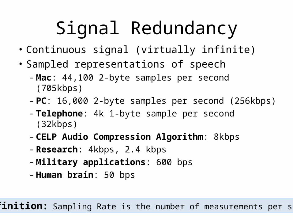
Signal Redundancy• Continuous signal (virtually infinite)• Sampled representations of speech

– Mac: 44,100 2-byte samples per second (705kbps)– PC: 16,000 2-byte samples per second (256kbps)– Telephone: 4k 1-byte sample per second (32kbps)– CELP Audio Compression Algorithm: 8kbps– Research: 4kbps, 2.4 kbps– Military applications: 600 bps– Human brain: 50 bps

Definition: Sampling Rate is the number of measurements per second

Noise

• Definition: Random electrical or acoustic activity that obscures communication

• Noise impact on speech– Noise degrades the speech recognition effectiveness– Consider construction noise outside the window– How much noise makes normal speech unintelligible?– What do human beings do to compensate?

• Automated Solution– Apply appropriate filters to eliminate noise from signals– Effective filters must not destroy essential signal data

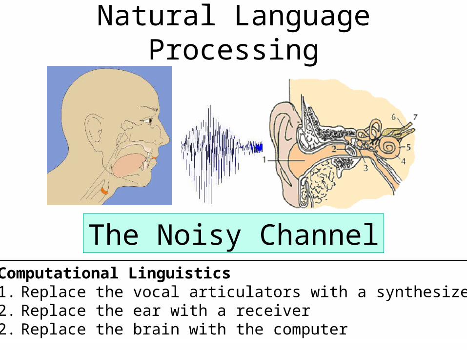
Natural Language Processing

The Noisy ChannelComputational Linguistics1. Replace the vocal articulators with a synthesizer2. Replace the ear with a receiver2. Replace the brain with the computer

Could a computer process this?I cdnuolt blveiee that I cluod aulaclty uesdnatnrd what I was

rdgnieg.

The phaonmneal pweor of the hmuan mnid Aoccdrnig to rscheearch at Cmabridgde Uinervtisy, it deosn't mttaer in what oredr the ltteers in a word are, the olny iprmoatnt tihng is that the frist and lsat ltteer be in the rghit pclae.

The rset can be a taotl mses and you can still raed it wouthit a problem.

This is bcuseae the huamn mnid deos not raed ervey lteter by istlef, but the word as a wlohe.

Amzanig huh?

Yaeh and I awlyas thought slpeling was ipmorantt!

Discrete versus Continuous• Continuous (analog): A signal, typically in found in nature,

whose infinite values are represented by a mathematical function. That is given any point in time, if we know the initial conditions, we can compute a value at that point.

• Discrete (digital): A sequence of measurements, each one separated by a fixed time interval.

• Digital processing of continuous signals– Computers deal with digital signals, because memory, though

large, has a finite size.– Input devices measure signal strength thousands of times a

second (e.g. audio: 44,100 is common). These values translate into a huge arrays in computer memory.

Signal Dimensionality

• Single Dimension (audio)

• Double Dimension (images)

• Three Dimensions (video)

• Higher Dimension (Climate Change Simulations)

Note: Even higher dimension signals can be reduced to a single dimension

Signal Power (Energy)

• Decibels: ratio between power of two signals. Dimensionless, like percent.

• SPL (Sound Pressure Level) is the ratio of a sound to the threshold of human hearing

Note: doubling the power increases decibels by three. Increase by 10 decibels increases power by 10.

Note: 10 log(P1/P2) = 20 log(A1/A2)

Understanding Digital Signal Processing, Third Edition, Richard Lyons(0-13-261480-4) © Pearson Education, 2011.

Energy is the square of the amplitude

Sound dB

TOH 0

Whisper 10

Quiet Room 20

Office 50

Normal conversation

60

Busy street 70

Heavy truck traffic 90

Power tools 110

Pain threshold 120

Sonic boom 140

Permanent damage

150

Jet engine 160

Cannon muzzle 220

Working with Signals• Special purpose languages: MatLab, Octave

– Matlab is very expensive, but available on campus– Octave, is largely compatible (but not entirely), and is free

• Free signal visualization programs: GraphCalc

• Sound Editing tools: ACORNS Sound Editor, Audacity. Sound Editor source is available to the class

• Java based resources: Java Sound, Tritonus

GraphCalc (Freeware )

Good for creating and visualizing signals

Communication of Signals• Pulse code Modulation (PCM)

– An array of measured values– Audio wav files: PCM with a header, defining big versus small

endian, sample rate, bytes per sample, number of channels

• Compression techniques to reduce bandwidth– Transmit differences between adjacent values– Don’t transmit runs of the same value– Algorithms (e.g. Linear prediction) to predict next values

from previous, and transmit the prediction errors– Coding techniques to transmit infrequent values using more

bytes than those that are common

Processing first step: translate compressed values to PCM

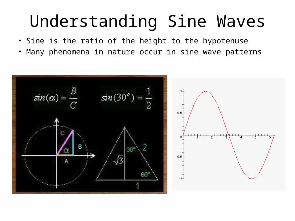
Understanding Sine Waves• Sine is the ratio of the height to the hypotenuse• Many phenomena in nature occur in sine wave patterns

Basic Terminology – periodic signals

• Amplitude — The distance from zero to the maximum height• Period — The time it takes for a sine wave to complete one cycle• Frequency (Hz) — The repetitions or cycles per second (1/period)

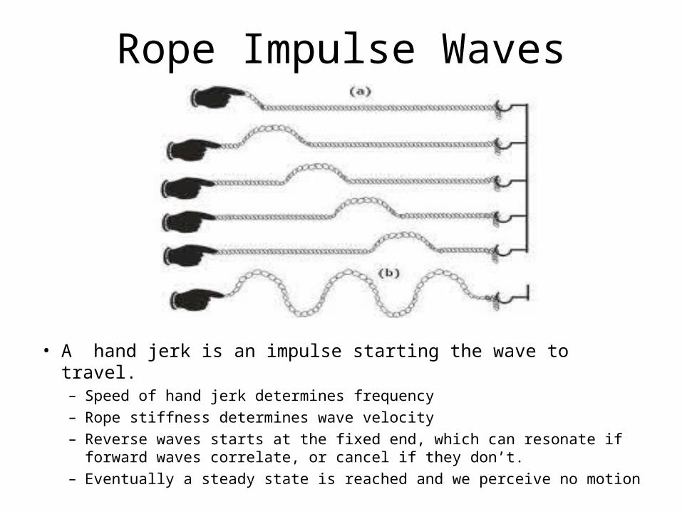
Rope Impulse Waves

• A hand jerk is an impulse starting the wave to travel. – Speed of hand jerk determines frequency– Rope stiffness determines wave velocity– Reverse waves starts at the fixed end, which can resonate if forward

waves correlate, or cancel if they don’t.– Eventually a steady state is reached and we perceive no motion

Traffic Waves

Complex Wave Patterns• Sound waves occupying the

same space combine to form a new wave of a different shape.

• Harmonically related waves add together and can create any complex wave pattern.

• Harmonically related waves have frequencies that are multiples of a basic frequency.

Note: All frequency waves do not have to start at zero, they can be “out of phase”. The amount of shift in degrees is called their phase angle.

Complex Wave Examples

Time vs. Frequency Domain

Time Domain: A composite wave summing different frequenciesFrequency Domain: Split time domain into component frequencies

Historical Note

• Jean Baptist Joseph Fourier (1768-1830)– Paper submitted: Academy of Science in Paris, 1807– Claim: All signals decompose into a sum of sine waves

• The review committee– Laplace (1749-1827) voted to accept– Lagrange (1736-1813) voted to reject. The claim did not

account for waves with sharp corners– The paper never got published

• Results– Fourier was correct if we use an infinite series of waves– Lagrange was correct if we use a finite series of waves– Fourier analysis is the foundation for Digital Signal

Processing (DSP)

Time and Frequency


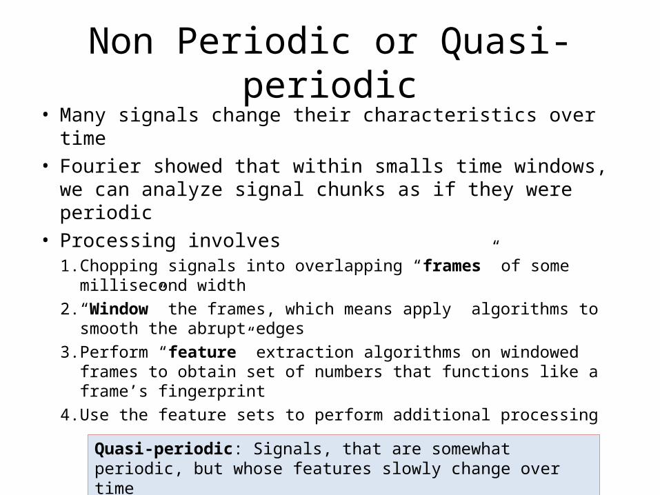
Non Periodic or Quasi-periodic• Many signals change their characteristics over time• Fourier showed that within smalls time windows, we can

analyze signal chunks as if they were periodic• Processing involves

1. Chopping signals into overlapping “frames” of some millisecond width

2. “Window” the frames, which means apply algorithms to smooth the abrupt edges

3. Perform “feature” extraction algorithms on windowed frames to obtain set of numbers that functions like a frame’s fingerprint

4. Use the feature sets to perform additional processing

Quasi-periodic: Signals, that are somewhat periodic, but whose features slowly change over time

Sample Sound Signal (Sound Editor)

Top: “this is a demo” Bottom: “A goat …. A coat”

Download and install from ACORNS web-site

Time Domain: x-axis: time, y-axis: amplitude measurement

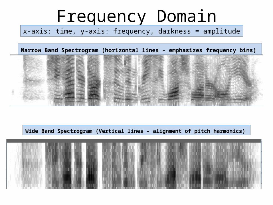
Frequency Domain

Narrow Band Spectrogram (horizontal lines – emphasizes frequency bins)

Wide Band Spectrogram (Vertical lines – alignment of pitch harmonics)

x-axis: time, y-axis: frequency, darkness = amplitude

Signal Power or Energy


Power is the square of the amplitude, often measured in decibels

Temporal Features• Advantages

– Minimal processing– Easy to understand

• Examples– Zero-crossing rate– Autocorrelation and autocorrelation peaks– Pitch periods– Loudness contour– Maximum and minimum distance between audio

positive and negative amplitude– Degree of voice in sounds (voicing quality)

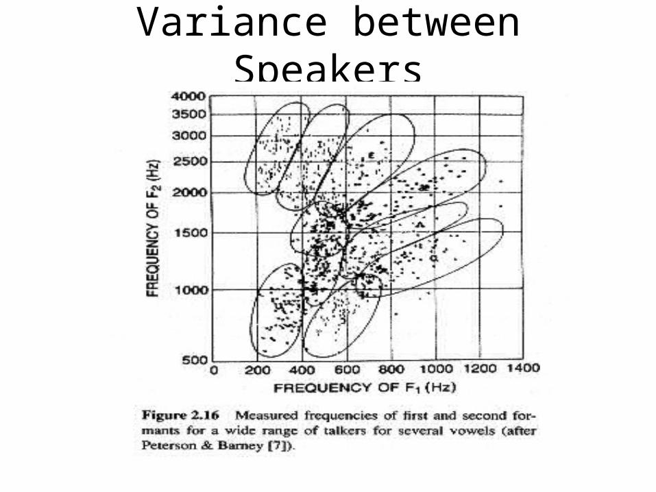
Variance between Speakers

Signal Filter


Modify the signal input in some way to produce a desired output

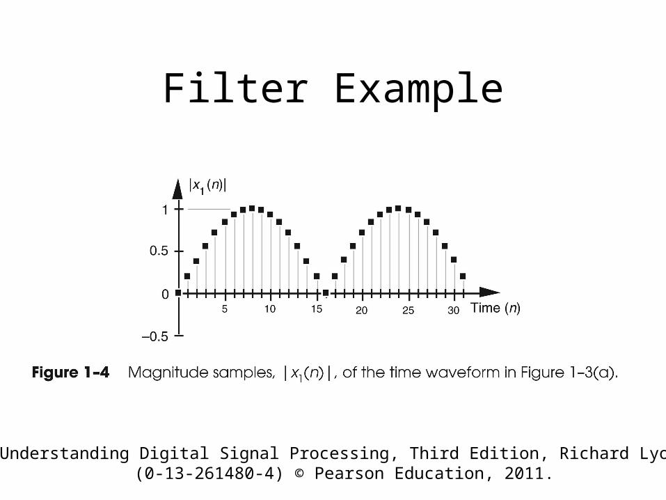
Filter Example


Moving Average Filter


Useful Examples: •A Crude low pass filter•Smoothing a speech pitch contour

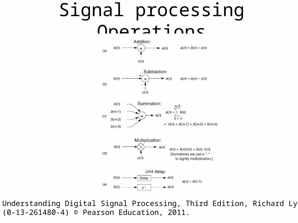
Signal processing Operations


Linear Systems

• If x1[n] ---> system ---> y1[n] andx2[n] ---> system ---> y2[n] where system manipulates the input values in some way

• A system is linear must be

– Homogeneous (output is the sum of its parts)c1*x1[n] + c2*x2[n] ---> system ---> c1*y1[n] + c2*y2[n]

– Time invariant (delay of input delays the output)x’1[n] = x[n+k] ---> system ---> y’1[n] = y[n+k]

Linear Systems

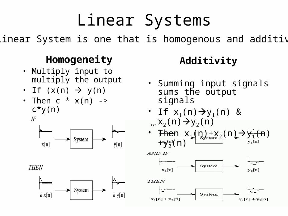
Homogeneity• Multiply input to multiply

the output• If (x(n) y(n)• Then c * x(n) -> c*y(n)

A Linear System is one that is homogenous and additive

Additivity

• Summing input signals sums the output signals

• If x1(n)y1(n) & x2(n)y2(n)• Then x1(n)+x2(n)y1(n)+y2(n)

Time Invariance

• Shift the input signal to identically shift the output• Assume: x(n)y(n)• Then: x(n+∆) y(n+∆)

Not required to be linear, but highly desirable

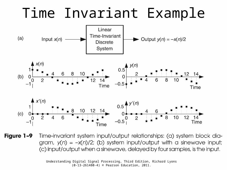
Time Invariant Example


Sinusoidal Fidelity

• Feed a sine wave to the input• Linear Systems

– Output will also be a sine wave– Output phase can shift– Output amplitude can be different

• Non-linear systems– Not likely to demonstrate sinusoidal fidelity– It is possible, however, for a non-linear system

to generate sine waves that don’t correlate to the input in a linear fashion

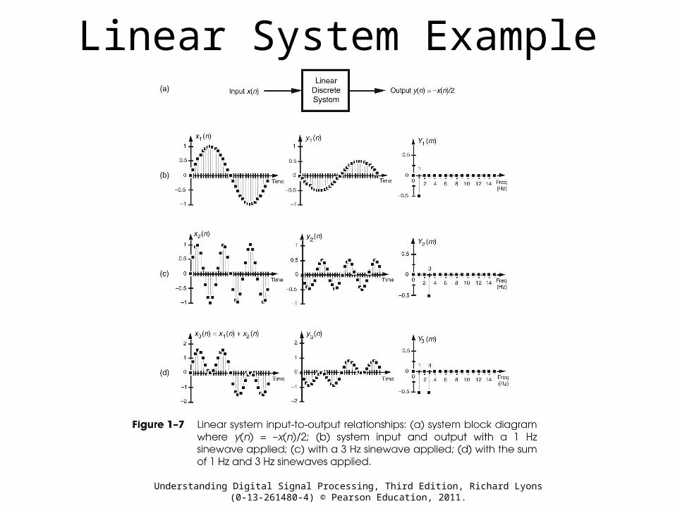
Linear System Example



Note: Linear systems can be connected in series and the result is still a linear system. Flipping the order of components does not affect the result because linear systems are commutative.


Note: Sending an impulse to an unknown system can help determine its operational characteristics

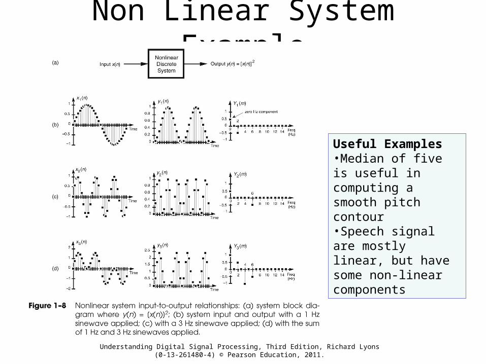
Non Linear System Example


Useful Examples•Median of five is useful in computing a smooth pitch contour•Speech signal are mostly linear, but have some non-linear components

How to Handle non-Linear Systems?

Approaches

• Ignore the non-linearity if it is small enough– Example: low levels of noise

• Convert to small amplitudes. – Many systems appear linear with small amplitudes

• Apply a linearizing transform– Assume a[n] = b[n] * c[n]

– Take logarithms (log(a[n] = log(b[n]) + log(c[n])

They must be linear for known ways of analysis

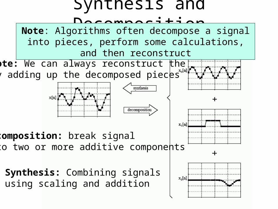
Synthesis and Decomposition

Decomposition: break signalinto two or more additive components

Synthesis: Combining signals using scaling and addition

Note: We can always reconstruct the by adding up the decomposed pieces

Note: Algorithms often decompose a signal into pieces, perform some calculations, and then reconstruct

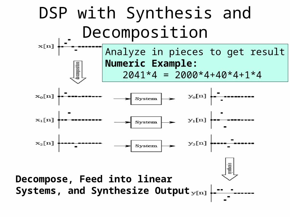
DSP with Synthesis and Decomposition

Decompose, Feed into linearSystems, and Synthesize Output

Analyze in pieces to get resultNumeric Example: 2041*4 = 2000*4+40*4+1*4

Even/Odd Decomposition

• Assumptions– Even number of total points (N)

– End sample attached to beginning

– Decompose into even and odd signal

• Even Symmetry– xE[n]= (x[n] + [N-n])/2

– Point 0 and N/2 = signal value

• Odd Symmetry– xO[N]= (x[n]-x[N-n])/2

– Point 0 and N/2 = 0

Interlaced Decomposition

• Decompose into even and odd signals

• Even signal contains zeroes in the odd indices

• Odd signal contains zeroes in the even indices

Digital Signal Processing What is a signal? a.An agreed upon message that triggers action or carries...

Documents

Transcript of Digital Signal Processing What is a signal? a.An agreed upon message that triggers action or carries...