Digital Pendulum Control Experiments

33-936S I

DIGITAL PENDULUM

Control Experiments

Digital Pendulum

Control Experiments

33-936S

Feedback Instruments Ltd., Park Road, Crowborough, East Sussex, TN6 2QX, UK

Telephone: +44 (0) 1892 653322, Fax: +44 (0) 1892 663719

email: [email protected] website: http://www.feedback-instruments.com

Manual: 33-936S Ed02-1 122013

Feedback Part No. 1160-33936S

33-936S II

DIGITAL PENDULUM

Control Experiments

33-936S III

DIGITAL PENDULUM

Control Experiments

Product Use

All users must familiarise themselves with the following information.

This product is marked as CE compliant. This means that it complies with the

relevant European Directives for this product. In particular the Directives cover Low

Voltage, EMC, Machinery, Pressure and electronic waste disposal.

The equipment, when used in normal or prescribed applications and within the

parameters set for its mechanical and electrical performance, should not cause any

danger or hazard to health or safety.

If, in specific cases, circumstances exist in which a potential hazard may be brought

about by careless or improper use, these will be pointed out and the necessary

precautions emphasised.

This equipment is designed for use by students as part of the learning process who

must be under the supervision of a suitably qualified and experienced person in a

laboratory environment where safety precautions and good engineering practices

are applied.

By the nature of its intrinsic teaching functionality, parts are visible and accessible

that might normally be covered up or encased in an industrial or domestic product.

For this reason students attention should be drawn to the need to operate the

equipment only in the manner prescribed in the accompanying documentation and

supervisors must make students aware of any particular risk. The equipment should

not be operated by any person alone.

We are required to indicate on our equipment panels certain areas and warnings

that require attention by the user. These have been indicated in the specified way by

yellow labels with black printing. The meanings of any labels that may be fixed to the

instrument are shown below:

CAUTION -

RISK OF

DANGER

CAUTION -

RISK OF

ELECTRIC SHOCK

CAUTION -

ELECTROSTATIC

SENSITIVE DEVICE

PREFACE

33-936S IV

DIGITAL PENDULUM

Control Experiments

Compliance with the EMC Directive

This equipment has been designed to comply with the essential requirements of the

Directive. However, because of the intrinsic teaching function it cannot be

electromagnetically shielded to the same extent as equipment designed for

industrial or domestic use. For this reason the equipment should only be operated in

a teaching laboratory environment where electromagnetic emissions in the

immediate area might not be expected to cause adverse effects. In the same way

users should be aware that operating the equipment near to an electromagnetic

source may cause the experimental results to be outside the range expected.

The Waste Electrical and Electronic Equipment Directive (WEEE)

If this equipment is disposed of it must be in accordance with the regulations

regarding the safe disposal of electronic and electrical items and not placed with

ordinary domestic or industrial waste.

Product Improvements

We maintain a policy of continuous product improvement by incorporating the latest

developments and components into our equipment, even up to the time of dispatch.

All major changes are incorporated into up-dated editions of our manuals and this

manual was believed to be correct at the time of printing. However, some product

changes which do not affect the teaching capability of the equipment, may not be

included until it is necessary to incorporate other significant changes.

Component Replacement

In order to maintain compliance with the Directives all replacement components

must be identical to those originally supplied.

Operating Conditions

This equipment is designed to operate under the following conditions:

Operating Temperature 10°C to 40°C (50°F to 104°F)

Humidity 10% to 90% (non-condensing)

WARNING:

This equipment must not be used in conditions of condensing humidity.

PREFACE

33-936S V

DIGITAL PENDULUM

Control Experiments

Copyright Notice

© Feedback Instruments Limited

All rights reserved. No part of this publication may be reproduced, stored in a

retrieval system, or transmitted, in any form or by any means, electronic,

mechanical, photocopying, recording or otherwise, without the prior permission of

Feedback Instruments Limited.

ACKNOWLEDGEMENTS

Feedback Instruments Ltd acknowledge all trademarks.

MICROSOFT, WINDOWS 8, WINDOWS 7 WINDOWS VISTA, WINDOWS XP, WINDOWS 2000, WINDOWS ME, WINDOWS NT, WINDOWS 98, WINDOWS 95 and Internet Explorer are registered trademarks of Microsoft Corporation.

MATLAB is a registered trademark of Mathworks Inc.

LabVIEW is a registered trademark of National Instruments.

PREFACE

33-936S VI

DIGITAL PENDULUM

Control Experiments

PREFACE

33-936S VII

DIGITAL PENDULUM

Control Experiments

Table of Contents

Manual overview ....................................................................................................... 1

Introduction ............................................................................................................... 2

Pendulum set description .......................................................................................... 3

Pendulum model ....................................................................................................... 5

Equations of motion ............................................................................................... 6

Exercise 1 – Nonlinear model ............................................................................. 7

Model linearisation .............................................................................................. 10

Exercise 2 – Linear models .............................................................................. 11

Model identification .............................................................................................. 12

Exercise 3 – Static friction compensation ......................................................... 13

Running a real-time model ............................................................................... 14

Dynamic Model.................................................................................................... 16

Cart model identification ...................................................................................... 17

Exercise 4 – Cart model identification .............................................................. 17

Crane identification .............................................................................................. 19

Exercise 5 – Crane linear model identification .................................................. 20

Inverted pendulum identification .......................................................................... 21

Exercise 6 – Inverted pendulum linear model identification .............................. 22

Pendulum setup control ........................................................................................... 26

Plant control ........................................................................................................ 27

PID controller ...................................................................................................... 28

Exercise 7 – PID control of cart model position ................................................ 29

Exercise 8 – Real time PID control of cart position ........................................... 31

Inverted pendulum control ................................................................................... 34

Control of pendulum swing-up ............................................................................. 34

Exercise 9 – Model swing up control ................................................................ 36

Exercise 10 – Real time pendulum swing up control ........................................ 36

Inverted pendulum stabilisation ........................................................................... 37

Exercise 11 – Pendulum stabilisation using the nonlinear model ...................... 39

Exercise 12 – Pendulum real time stabilisation................................................. 39

Crane control ....................................................................................................... 41

Exercise 13 – Crane control ............................................................................. 42

Combined control techniques .............................................................................. 42

Swing up and hold ............................................................................................... 42

Exercise 14 – Swing up and hold control .......................................................... 43

Up and down ....................................................................................................... 44

Exercise 15 – Up and down.............................................................................. 44

Detailed description of the Up/Down model ............................................................. 46

TABLE OF CONTENTS

33-936S VIII

DIGITAL PENDULUM

Control Experiments

33-936S 1

DIGITAL PENDULUM

Control Experiments

Manual overview

The following manual refers to the Feedback Instruments Digital Pendulum Control

application. It serves as a guide for the control tasks and provides useful information

about the physical behaviour. In the manual a model is proposed and linearisation is

introduced. Identification algorithms are proposed and the models obtained are

compared with phenomenological models. Control algorithms are developed and

tested on the pendulum models and then implemented in a real time application.

Throughout the manual various exercises are proposed to bring the user closer to the

pendulum control problem. Depending on the knowledge level of the user some of

the sections and exercises can be skipped. The more advanced users can try to

model, identify and control the pendulum on their own from the beginning.

If any of the identification or controller design exercises appear to be too difficult or

the results are not satisfactory, you can use the ready-made control applications that

are supplied and test them by changing the parameters of the controllers.

The relative difficulty of each exercise is indicated using the following icons:

� easy level,

� medium level,

� expert level.

MANUAL OVERVIEW

33-936S 2

DIGITAL PENDULUM

Control Experiments

Introduction

The pendulum workshop can be divided into two separate control problems. First is

the crane control problem, in which the goal is to move the cart into a desired

position with as little oscillation of the load (pendulum arms) as possible. The other is

to stabilize the inverted pendulums in an upright position. The crane control problem

is very often encountered in industrial applications where load movement is

incorporated. It is especially difficult to realise when cranes are placed on ships and

the effect of waves is considered.

The inverted pendulum task can be seen as a self-erecting control problem, which is

present in missile launching and control applications. Furthermore the pendulum

application involves a swing-up control aspect if initially the pendulum hangs freely in

the vertical position.

These two control problems (inverted pendulum and crane control) have one very

important difference, which is the stability. The pendulum serving as a crane is stable

without a working controller. Due to energy loss through friction and air resistance it

will always end up at an equilibrium point.

The inverted pendulum is inherently unstable. Left without a stabilizing controller it

will not be able to remain in an upright position when disturbed.

INTRODUCTION

33-936S 3

DIGITAL PENDULUM

Control Experiments

Pendulum set description

The description of the pendulum setup in this section refers mainly to the control

problems. For connection, interface and an explanation of how the signals are

measured and transferred to the PC, refer to the ‘Installation & Commissioning’

manual.

As shown in Figure 1 the pendulum setup consists of a cart moving along the 1 metre

length track. The cart has a shaft to which two pendulums are attached and are able

to rotate freely. The cart can move back and forth causing the pendulums to swing.

Figure 1 Digital Pendulum mechanical unit

The movement of the cart is caused by pulling the belt in two directions by the DC

motor attached at the end of the rail. By applying a voltage to the motor we control

the force with which the cart is pulled. The value of the force depends on the value of

the control voltage. The voltage is our control signal. The two variables that are read

from the pendulum (using optical encoders) are the pendulum position (angle) and

PENDULUM SET DESCRIPTION

33-936S 4

DIGITAL PENDULUM

Control Experiments

the cart position on the rail. The controller’s task will be to change the DC motor

voltage depending on these two variables, in such a way that the desired control task

is fulfilled (stabilizing in an upright position, swinging or crane control).

Figure 2 presents how the control system is organised.

Figure 2 Pendulum control system

In order to design any control algorithms one must understand the physical

background behind the process and carry out identification experiments. The next

section explains the modelling process of the pendulum.

PENDULUM SET DESCRIPTION

33-936S 5

DIGITAL PENDULUM

Control Experiments

Pendulum model

Every control project starts with plant modelling, so as much information as possible

is given about the process itself. The mechanical model of the pendulum is presented

in Figure 3.

Figure 3 Pendulum phenomenological model

The phenomenological model of the pendulum is nonlinear, meaning that at least one

of the states (x and its derivative or θ and its derivative) is an argument of a nonlinear

function. For such a model to be presented as a transfer function (a form of linear

plant dynamics representation used in control engineering), it has to be linearised.

PENDULUM MODEL

33-936S 6

DIGITAL PENDULUM

Control Experiments

Equations of motion

Summing the forces acting on the pendulum and cart system and the moments we

obtain the following nonlinear equations of motion:

0cossin

sincos)(

2

2

=++−+

=−+++

θθθθ

θθθθ

&&&&&

&&&&&&

dxmlmgl)ml(I

FmlmlxbxMm

Very often control algorithms are tested on such nonlinear models. However for the

purpose of controller design the models are linearised and presented in the form of

transfer functions. Such a linear equivalent of the nonlinear model is valid only for

small deviations of the state values from their nominal value. Such a nominal value is

often called the equilibrium point. The pendulum has two of these, one is when θ = 0

(inverted pendulum) and the other when θ = π (hanging freely – crane control).

The inverted pendulum is an unstable system which, in terms of behaviour, means

that the plant left without any controller reaches an unwanted, very often destructive

state. Thus for such plants it is useful to carry out simulation tests on the models

before approaching the real plant.

To complete the model given by motion equations (1) and (2), we must introduce the

values of all parameters. The following table gives these values:

Figure 4 Pendulum parameters

Two things have to be kept in mind when designing the controllers. Both the cart

position and the control signal are bounded in a real time application. The bound for

the control signal is set to [–2.5V .. +2.5V] and the generated force magnitude of

(1)

(2)

PENDULUM MODEL

33-936S 7

DIGITAL PENDULUM

Control Experiments

around [–20.0N .. +20.0N]. The cart position is physically bounded by the rail length

and is equal to [-0.5m .. +0.5m].

The pendulum is a SIMO plant – single input multiple output (Figure 5). The model

described by equations (1) and (2) is still missing the translation between the force F

and the actual control signal, which is the control voltage u that we supply with the

PC control card. Assuming that the relation between the control voltage u and the

generated cart velocity is linear, we might add the velocity vector generated by the

motor to the model and ignore the F vector, or translate the control voltage u to the

generated force F under the assumption that constant voltage will cause the cart to

move with constant velocity:

,dt

dukF Fu ⋅=

where kFu is the gain between the u voltage derivative and the F force. However one

must remember that derivative introduction in models especially in Simulink may

cause simulation problems.

Figure 5 Pendulum model

Exercise 1 – Nonlinear model

Introduction

For the initial exercise the user has been provided with the pendulum model

described by equations (1) and (2). The model shown in Figure 5 can be

opened in Simulink. The model is called pendmod_nonlin.mdl and it can be run

by navigating using the Windows start menu (Figure 6):

Start menu→All Programs→Feedback Instruments→Feedback 33-936…→Simulink Models

Figure 6 Start menu

(3)

PENDULUM MODEL

33-936S 8

DIGITAL PENDULUM

Control Experiments

Matlab will run and a Simulink menu will be displayed (Figure 7). Double click

Pendulum Simulation Models then double click the appropriate model in the

next selection window.

Figure 7: Model category window

Task

To begin with the user is advised to check the responses of the model in the

situation where zero u voltage is applied (i.e. the cart is not driven). You can

change the value of θ0 (the initial pendulum angle) and see how the pendulum

responds. To change the initial pendulum angle double click the ‘Pendulum

with DC motor’ block then double click the ‘Pendulum’ block to gain access to

its parameters. If you wish to explore the pendulum model further, right click on

the block and select ‘Look under mask’.

Example results and comments

Two values of the angle θ0 are particularly interesting: θ0 = 0 and θ0 = π. The

first is an equilibrium point for which a small disturbance of an open loop

system will cause the pendulum to fall down, swing and finally settle down with

θ =π. The small disturbance can be introduced by small initial angle selection,

for example θ0 = 0.001. The second θ0 = π is an equilibrium in which the

pendulum will always settle when no F force is applied.

PENDULUM MODEL

33-936S 9

DIGITAL PENDULUM

Control Experiments

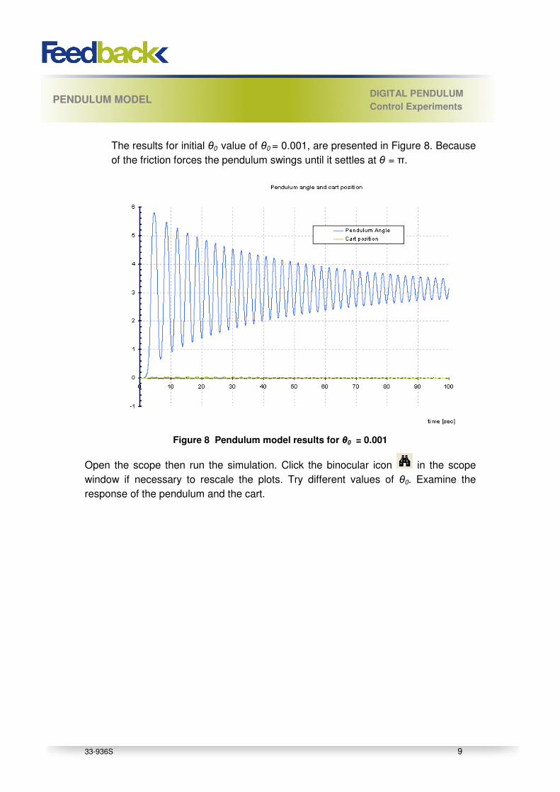
The results for initial θ0 value of θ0 = 0.001, are presented in Figure 8. Because

of the friction forces the pendulum swings until it settles at θ = π.

Figure 8 Pendulum model results for θ0 = 0.001

Open the scope then run the simulation. Click the binocular icon in the scope

window if necessary to rescale the plots. Try different values of θ0. Examine the

response of the pendulum and the cart.

PENDULUM MODEL

33-936S 10

DIGITAL PENDULUM

Control Experiments

Model linearisation

To carry out analysis of the model dynamics for open loop1 systems using techniques

such as Bode plots, poles and zeros maps, Nyquist plots, root locus (for closed loop2

systems only), the model has to be linearised. Linearisation of a given

phenomenological model can be carried out for the pendulum and in equations (1)

and (2) we could substitute the nonlinear functions (sine and cosine) with their linear

equivalent. Such a linearisation of a working point is done with a Taylor

approximation of the nonlinear functions. For small angle deviations around an

equilibrium point of θ = 0 (inverted pendulum) we can assume that the following

functions can be linearised:

.0

,1cos

,sin

2=

≅

≅

θ

θ

θθ

&

Thus the motion equations (1) and (2) take the form:

.0

,)(

2=++−+

=+++

θθθ

θ

&&&&&

&&&&&

dxmlmgl)ml(I

FmlxbxMm

One must remember that the equations (7) and (8) will only be valid around the

position where θ = 0. For the position where θ = π (crane control) the following

substitutions have to be made:

.0

,1cos

,sin

2=

−≅

−≅

θ

θ

θθ

&

Thus the motion equations (1) and (2) take the form:

.0

,)(

2=+−++

=−++

θθθ

θ

&&&&&

&&&&&

dxmlmgl)ml(I

FmlxbxMm

1 Open loop system – the plant without a controller

2 Closed loop system – the plant and controller with a negative feedback loop, see “Control”

section for more information.

(4)

(5)

(6)

(7)

(8)

(9)

(10)

(11)

(12)

(13)

PENDULUM MODEL

33-936S 11

DIGITAL PENDULUM

Control Experiments

The linear model of the pendulum, just as the nonlinear model, has one input which

is the force F, and two outputs which are the pendulum angle θ and the cart position

x (Figure 5). However, in the inverted pendulum task we are mostly interested in the

θ angle stabilisation thus we may treat the cart position as an uncontrolled output.

With one input F and one output θ, two linear models in the form of transfer functions

can be obtained, each for small deviations of the θ angle from the two equilibrium

points of θ = [0, π]. Remember that the translation between the control voltage and

the force should be added (equation 3).

Exercise 2 – Linear models

Introduction

Two of the linear models described by the equations (7),(8) and (12),(13) have

been created for you called pendmod_lin_unstable.mdl (inverted pendulum)

and pendmod_lin_stable.mdl (crane) respectively. The user is advised to

transform (7),(8) and (12),(13) into transfer function form as an exercise.

One must remember that both of these transfer functions resemble the

behaviour of the real plant only for small deviations of the θ angle. The models

pendmod_lin_stable.mdl and pendmod_lin_unstable.mdl hold the appropriate

transfer functions:

01

2

2

3

3)(

)()(

dsdsdsd

s

sF

ssG

+⋅+⋅+⋅==

θ

For both of these models the signs of the denominator parameters will differ.

The x position output is calculated based upon the output of the G(s) transfer

function, which is θ. For the stable transfer function (i.e. the representation of

the pendulum behaviour in the region where θ = π), an offset of offset = π has to

be added to the output of the transfer function. That is our initial condition.

Figure 9 Example of the linear Simulink model

(14)

PENDULUM MODEL

33-936S 12

DIGITAL PENDULUM

Control Experiments

Task

Run the linear (pendmod_lin_unstable.mdl) & nonlinear (pendmod_nonlin.mdl)

pendulum models in an open loop system (no controller) and compare the

responses. Also, with the use of Matlab, the Bode diagrams, zeros and poles

maps can be drawn to carry out initial dynamic response analysis of the

pendulum.

In the transfer function form of the model the initial condition is equal to zero

thus in order to see the linear model response we have to stimulate it with a

control voltage pulse to see the reaction. Inspection of the voltage pulse block

in either model will show that the system is given a momentary 0.1V ‘kick’ at

time t=0 so that the response can be observed.


The dynamic response of the linearised unstable transfer function

pendmod_lin_unstable.mdl will be different from the nonlinear system

pendmod_nonlin.mdl. When disturbed by a small voltage impulse u, the

unstable system will not settle at equilibrium with θ = π. The linearised transfer

function is only valid for small deflections of θ thus it is unstable and the

response grows to infinity without any control action.

The stable (crane) transfer function pendmod_lin_stable.mdl is also only valid

for small deviations of θ but for an equilibrium of θ = π, it will behave similarly to

the nonlinear model around the point θ = π.

Model identification

The phenomenology analysis delivers a model that we ‘think’ fits the pendulum the

best. However we know that it is just some approximation. We might have made

mistakes analysing the phenomenology and, for example, chosen the wrong model

structure or incorrect parameter values. To have an adequate model we could tune

the phenomenological model. Because of the fact that it is nonlinear, the

identification and tuning of that model can be a very difficult task (gradient methods).

To simplify the identification, modelling and control, the control algorithms will be

designed based upon the dynamics of the linear models. They will be tested however

on the nonlinear model and plant. Furthermore the identified models will be discrete

as such models are obtained in the course of the Least Mean Square identification

methods implemented in Matlab. Any of the continuous models can also be

transformed for comparison purposes into the discrete form. The discrete models

obtained can be also transformed into the continuous equivalent.

PENDULUM MODEL IDENTIFICATION

33-936S 13

DIGITAL PENDULUM

Control Experiments

Plant identification theory is very broad and solves numerous problems. In the

identification experiments of the linear pendulum models it is convenient however to

use the Matlab identification tool.

Before any model identification procedures of the pendulum setup are carried out, we

have to describe, through a simple real-time simulation, the character of the dead

zone. The dead zone is a nonlinearity, which could influence the model validity.

Because of the static friction forces (also called stiction), with very small values of

control signal the cart will not move. Furthermore the static friction force may not be

symmetrical. We can compensate for that simply by adding an additional voltage

offset value to the cart control signal. Measurement of the value of the offset is the

purpose of Exercise 3.

Exercise 3 – Static friction compensation

Introduction

Since the control signal is the voltage that we supply to drive the cart motor, the

dead zone value will be expressed in volts. As explained previously, it is likely

to be different for the two directions of movement. It has to be identified

because the tension of the pendulum motor belt can be set up differently by the

user and thus cause significantly different static friction forces. The

measurement of static friction can be carried out using the real-time model

PendulumFriction.mdl. In the simulation the control voltage is increased until

the cart moves in the positive direction. The cart is stopped. Then the control is

reversed and increased until the cart moves in the negative direction. The

voltage values for which the cart begins to move are recorded and can be used

in the controller to compensate for static friction.

Task

Run the friction identification simulation on the pendulum. Unlike the previous

models which were non real-time simulations and did not require access to real

hardware, this model runs in real-time and interfaces with the Pendulum

Mechanical unit using an I/O card installed in the PC and the Digital Pendulum

Controller.

The model is called PendulumFriction.mdl and it can be run from the Simulink

menu by double clicking the Pendulum Real-time models block.


33-936S 14

DIGITAL PENDULUM

Control Experiments

The real-time models provided with the Feedback 33-936 software must be

built before they can be executed in real-time. If the model is not already built,

select the Tools menu then Real-Time Workshop and Build Model (Figure 10).

Figure 10 Building a model

Go to the Matlab command window to observe the progress of the build. When

the build is complete, check that it was successful (i.e. no error messages were

displayed in the command window).

You are now ready to run the model.

Running a real-time model

The following sequence is very important and should always be followed when

preparing to execute a real-time model.

1. Make sure that before you run the application, the Digital Pendulum

Controller POWER switch is ON but the green START pushbutton is

OFF (the green pushbutton lamp is not illuminated). If necessary, press

the red STOP pushbutton.

2. Place the cart in the centre of the track (over the marker) and stop the

pendulum from swinging.

3. Connect the application with the target by pressing the Connect to

Target button or using the External Mode Control Panel from the

Tools menu of the Simulink window. The application will not run yet but


33-936S 15

DIGITAL PENDULUM

Control Experiments

the PCI-1711 card will be initialised correctly. Confirm that the

application is connected by the scrolling activity indicator at the bottom

of the Simulink model window. Now press the green START pushbutton

on the Digital Pendulum Controller unit.

4. If the area around the pendulum is clear you can start the application by

pressing the Start Real Time Code button or using the External

Mode Control Panel.

5. When the simulation is complete, press the red STOP button on the

Digital Pendulum Controller.

6. If you wish to stop a simulation part way through, press the red STOP

switch on the Digital Pendulum Controller first. Then stop the simulation

using the Simulink controls. To restart, follow the steps above again.

Follow the steps above and run the PendulumFriction.mdl model. The signal to

the cart motor will be increased until the cart just moves and then its value will

be recorded. The sequence is then repeated in the opposite direction.


The results of the static friction measurements will be presented in two

displays. You can use these measured values to correct the friction

compensation value in all future simulations. The compensation values are

stored in the ‘Friction Compensation’ block (Figure 11, Figure 12), which is

located within the ‘Feedback DAC’ block of each controller model. However if

the result of the test is significantly greater than ±0.2V it may appear to be

biased by other nonlinearities and should be investigated further.

Figure 11 Friction compensation block

PENDULUM MODEL IDENTIFICATION PENDULUM MODEL IDENTIFICATION

33-936S 16

DIGITAL PENDULUM

Control Experiments

Figure 12 Friction compensation block parameters

Dynamic Model

With the static friction identification carried out we can try to identify the first dynamic

model of the pendulum. Although the most interesting signal relation is the one

between the control signal u and the angle θ we can first try to identify the linear

model between the control signal u and the cart position x. That model will be used

for first PID controller design and tested in the Pendulum control section.

There are a few important things that the control system designer has to keep in

mind when carrying out an identification experiment:

� Stability problem – if the plant that is identified is unstable, the

identification has to be carried out with a working controller which

introduces additional problems that will be discussed further on. If the

plant is stable and does not have to work with a controller the

identification is much simpler.

� Structure choice – a very important aspect of the identification. For the

linear models it comes down to the choice of the numerator and

denominator order of the transfer function. It applies for both the

continuous and discrete systems.

As far as the discrete models are concerned the structures are also

divided in terms of the error term description: ARX, ARMAX, OE, BJ3.

� Sampling time – the sampling time choice is important for both

identification and control. It cannot be too short nor can it be too long.

Too short sampling time might influence the identification quality

3 More information about these structures can be obtained as part of a System Identification

course.

33-936S 17

DIGITAL PENDULUM

Control Experiments

because of the quantisation effect introduced by the A/D converter.

Furthermore the shorter the sampling time the faster the software and

hardware has to be and more memory is needed. However short

sampling time will allow for elimination of aliasing effects and thus anti

aliasing filters4 may not be needed. Long sampling times will not allow

for including all of the dynamics.

� Excitation signal – for linear models the excitation choice is simple. Very

often designers use white noise, however in industrial applications it is

often disallowed. It is attractive because it holds a very broad frequency

content thus the whole dynamics of the plant can be identified. If the

dynamics are not too complex, several sinusoids with different

frequencies can be summed to produce a satisfactory excitation signal.

� Identification method – usually two methods are used, the Least Mean

Square (LMS) method and the Instrumental Variable method. The LMS

method is the most popular and is implemented in Matlab. This method

minimizes the error between the model and plant output. The optimal

model parameters, for which the square of the error is minimal is the

result of the identification.

Cart model identification

The following exercise takes into account the facts mentioned above and provides an

identification experiment, which results in a discrete model of the moving cart due to

the application of the control voltage. At this point the pendulum is ignored; its

movement is treated as a distortion. It would be best to immobilize the pendulum to

reduce the disturbance.

Exercise 4 – Cart model identification

Introduction

All of the control real-time simulations are carried out with a sampling time of

Ts = 0.001[s]. In the identification experiments the sampling time varies. For

this identification the Matlab identification interface is used. Here the sampling

time is set to Ts = 0.05[s].

4 These are the basics of a Digital Signal Processing course. For more insight the user is

asked to study more on signal processing and digital control.


33-936S 18

DIGITAL PENDULUM

Control Experiments

The identification experiment is carried out with the model CartIdent.mdl. The

excitation signal is composed of several sinusoids and an optional random

signal block, which output can be added to the excitation. You can check the

effect of the additional random signal on the identification results. However one

must be careful with the choice of random signal parameters as extensive

random signals are destructive for the actuator. The experiment lasts 20

seconds and signals are collected in a form of vectors and are available in the

Matlab workspace. The signals are cart position, pendulum angle, motor control

voltage and a time reference.

Task

Carry out the identification experiment by running CartIdent.mdl and collecting

the data. When the run is complete, press the red STOP pushbutton on the

Digital Pendulum Controller unit.

Reduce the slider gain value if the cart hits the limit switch during the

identification experiment or improve stiction compensation.

Analyse the results using the Matlab identification interface (part of the System

Identification Toolbox). You will notice that a new workspace variable simout

has been created which contains the signals listed above.

For simplicity assign the input and output data to the u and y vectors

respectively:

u = simout(:,3);

y = simout(:,1);

For instructions on identification experiments refer to the ‘Matlab Guide’

manual.

One of the possible model structure and order choices is the oe241.


33-936S 19

DIGITAL PENDULUM

Control Experiments

Figure 13 Step response


The step response of the identified system should be similar to the one

presented in Figure 13. If the model is transferred into the Workspace it can be

compared against the discrete equivalent of the continuous transfer function. In

order to obtain the discrete form use the ‘c2d’ command. Make sure you

specify the proper sampling time.

Compare the step responses or bode plots of the two systems (using ‘step’ and

‘bode’ commands). You can also transform the discrete models into continuous

equivalent with the means of ‘d2c’ command.

The model obtained is used in the first PID control exercise.

Crane identification

A similar identification experiment can be carried out for the Crane mode to identify

the transfer function between the control voltage u and the pendulum angle θ. As

presented in the Model linearisation section, two linear models can be identified. The

first which holds for small deviations of angle θ around the θ=0 point, and the other

when θ=π. In this section the crane function of the pendulum is considered, thus

θ=π.


33-936S 20

DIGITAL PENDULUM

Control Experiments

Exercise 5 – Crane linear model identification

Introduction

The crane linear discrete model can be identified in the same way as the cart

model (Exercise 4), using the Matlab System Identification Toolbox. The

identification experiment is carried out with the model CraneIdent.mdl. The

excitation signal is composed of several sinusoids. The experiment lasts 100

seconds in total. The excitation signal is applied for the first 10 seconds then

the pendulum is allowed to swing freely for 80 seconds to identify the damping

effect. Signals are collected in a form of vectors which are available in the

Matlab workspace. The signals are cart position, pendulum angle, motor control

voltage and a time reference. The sampling time is set at Ts = 0.05 [s].

Task

Carry out the identification experiment by running CraneIdent.mdl and

collecting the data. When the run is complete, press the red STOP pushbutton

on the Digital Pendulum Controller unit.


respectively:

u = simout(:,3);

y = simout(:,2);

With the use of the Matlab identification interface, identify a discrete model.

Import the data and run the estimation as described in Matlab Guide manual.

Select the proper structure of the model (e.g. OE 2 6{or higher} 1). You can

check the quality of the response of the identified model by the step response

analysis, transient response, pole and zeros map, frequency response and

model residuals.


The response of the model is compared to the pendulum output in Figure 14. If

the model is transferred into the Workspace it can be compared against the

discrete equivalent of the continuous transfer function (14). In order to obtain

the discrete form use the ‘c2d’ command. Make sure you specify the proper

sampling time.

The models you obtain may strongly depend on the mounting of the belt and

the tightness of all fixings.


33-936S 21

DIGITAL PENDULUM

Control Experiments

Figure 14 Identified model and pendulum response to excitation

Drag the oe241 model icon to the To Workspace box to export it to a

workspace variable. Save the session using the File→ Save session as.. menu.

Inverted pendulum identification

Inverted pendulum model identification is a difficult task mainly for one aspect –

stability. The inverted pendulum is unstable and has to be identified with a running,

stabilising controller5 i.e. closed loop identification6. The controller introduces output

noise and control signal correlation, which leads to model corruption. This correlation

can be broken by introducing an additional excitation signal r, which is added to the

control signal u (Figure 15).

If the power of the signal r is substantial compared to the noise power n, the proper

model should be identified.

5 The pendulum control aspect is explained in the ‘Pendulum Control’ section.

6 Closed loop system identification is a broad topic and more advanced users are advised to

refer to identification literature to get more insight.


33-936S 22

DIGITAL PENDULUM

Control Experiments

Figure 15 Unstable system identification

Such an approach will only allow for the linear model identification of the transfer

function between the voltage control signal u and the pendulum angle θ, for small

deviations of the angle around the equilibrium point of θ = 0.

More intelligent identification methods should be applied for complete nonlinear

pendulum model identification (gradient methods).

A closed-loop system describing the relation between signal r and y is identified:

)()(1

)()(

11

11

−−

−

−

⋅+=

zGzC

zGzT ,

where T( 1−z ) is the complete system discrete transfer function describing the relation

between, C( 1−z ) is the discrete controller transfer function and G( 1−z ) is the

pendulum model discrete transfer function. The relation (15) can be transformed to

yield the pendulum model:

)()(1

)()(

11

11

−−

−

−

⋅−=

zTzC

zTzG

Such approach is presented in Exercise 6 to yield a complete inverted pendulum

model.

Exercise 6 – Inverted pendulum linear model identification

Introduction

The linear discrete model of the inverted pendulum can be identified only with a

controller. This is a major difference compared to the previous exercises.

(15)

(16)


33-936S 23

DIGITAL PENDULUM

Control Experiments

The identification experiment is carried out with the model InvPendIdent.mdl.

The excitation signal is composed of several sinusoids. The experiment lasts

40 seconds in total. Signals are collected in a form of vectors which are

available in the Matlab workspace. The signals are pendulum angle, motor

control voltage, cart position and a time reference. The sampling time is set at

Ts = 0.001 [s].

It is IMPORTANT that before the identification experiment is started, you place

the cart in the ZERO position and settle the pendulum in the bottom vertical

position, θ = π.

Task

Carry out the identification experiment by running InvPendIdent.mdl and

collecting the data.

Caution: Keep well clear of the pendulum when running the model

When the run is complete, press the red STOP pushbutton on the Digital

Pendulum Controller unit. The pendulum response to the excitation will be as

presented in Figure 16.

Figure 16 Pendulum response


33-936S 24

DIGITAL PENDULUM

Control Experiments


respectively:

u = simout(:,5);

y = simout(:,1);

For instructions on identification experiments refer to the ‘Matlab Guide’

manual.

With the use of the Matlab identification interface, identify a discrete model of

the whole system together with controller - T(z-1). Specify the proper sampling

time which is Ts=0.001s for this example. Select the proper structure of the

model (e.g. OE 3 6 1 or higher) then estimate.

After identifying the transfer function of the whole system with controller extract

the plant model according to equation (16). Use the Mextract.m file to perform

that transformation. Type ‘help Mextract’ to view help on this file. The model is

also transformed into a continuous form.

Make sure that for the model identification you use the data from the time when

the pendulum is in the upright position. Referring to the example plot (Figure

16), it is safe to use data from around the 9 seconds onwards in this case.

Different mechanical units will have a different swing-up time so either plot the

position vs. time using:

plot (simout(:,4), simout(:,1)) to check, or use a larger figure (e.g. 15 seconds)

to be sure to avoid the swing-up region.

Import the data as usual using a start time of 0. The time range of the imported

data can then be selected using Preprocess ->Select Range… Enter the start

time (say 15) in the Time span box then hit Enter then select Insert and Close.

The new dataset will appear. Drag the new dataset into the Working Data box.

You can check the quality of the response of the identified model by the step

response analysis, transient response, pole and zeros map, frequency

response and model residuals.


33-936S 25

DIGITAL PENDULUM

Control Experiments


The response of the identified closed loop system T(z-1) can be easily

compared with the plant response to express the identification quality (Figure

17). It is impossible to compare the model of the unstable plant itself unless

nonparametric methods are incorporated in the identification task.

The model obtained will be used in the ‘Pendulum Control’ section for the

controller design.

Figure 17 Inverted pendulum model vs plant response


33-936S 26

DIGITAL PENDULUM

Control Experiments

Pendulum setup control

The pendulum control aspect covers three control areas:

� crane control,

� inverted pendulum control,

� swing up control.

Each of these control problems has its particular characteristic. As mentioned in the

introduction the pendulum is a nonlinear plant, thus control over a wide range of

angles by one simple linear controller is impossible. The nonlinear pendulum model

has been linearised (Model linearisation section) to give two separate models for the

upright and hanging pendulum position. Corresponding models have been also

obtained in the course of the identification experiments as described in the Model

identification section. Based on these linear models, simple control algorithms can be

designed, one of which is the very widely used PID controller.

The plant itself is called an open loop system (Figure 18) that means it has no

controller. The pendulum can be treated as a SISO or SIMO system depending on

how many states we want to control.

Figure 18 Pendulum

Matlab provides various analysis methods for linear systems as far as dynamics are

concerned (root locus, frequency analysis tools – Bode diagrams, Nyquist plots, pole

and zero maps etc.). Controllers can be designed using the information which Matlab

provides about the dynamics of the system. The following sections explain how the

PID controller works and how it can be tuned.

PENDULUM SETUP CONTROL

33-936S 27

DIGITAL PENDULUM

Control Experiments

Plant control

There are numerous control algorithms however PID control is the most popular

because of its simplicity. A general schematic of a simple closed loop control system

is presented in Figure 19.

Figure 19 Simple closed-loop control system

Assuming that the plant is represented by its linear model its transfer function can be

described as:

)(

)()(

sA

sBsG =

where s is the Laplace operator. The idea of control algorithms is to find such a

controller (transfer function, discrete transfer function, any nonlinear), which will fulfil

our requirements (certain dynamic response, certain frequency damping, good

response to the dynamic changes of the desired value etc.). The controller input is

the e(t) error signal. Sometimes disturbance signals are also measured. Depending

on the present and past values of the error signal, the controller performs such an

action (changes the u(t) control signal) so that the y(t) is as close as possible to the

ydesired(t) value at all times.

There are many controller design and tuning methods. All of them consider the

behaviour of the closed loop system (plant with a controller as in Figure 19) and

provide controller parameters according to the assumed system characteristics. With

the known plant transfer function G(s) it is possible to find satisfactory parameters of

the C(s) controller such that the closed loop system will have the desired

characteristics described by the transfer function Tc(s):

)()(1

)()()(

sGsC

sGsCsTc

⋅+

⋅=

(17)

(18)


C(s) G(s)

33-936S 28

DIGITAL PENDULUM

Control Experiments

PID controller

A PID controller consists of 3 blocks: Proportional, Integral and Derivative. The

equation governing the PID controller is as follows:

)()()(

)()()()(

tytyte

dt

tdeDdtteItePtu

desired −=

⋅+⋅+⋅= ∫

By means of the Laplace transform such a structure can be represented as a transfer

function:

s

IPsDssD

s

IP

sE

sUsC

sEsDs

IPsU

++=⋅++==

⋅⋅++=

2

)()(

)()(

)()()(

Each block of the PID controller plays an important role. However for some

applications, the integral or derivative part has to be excluded to give satisfactory

results. The proportional block is mostly responsible for the speed of the system

reaction. However for oscillatory plants it might increase the oscillations if the value

of P is set to be too large.

The integral part is very important and assures zero error value in the steady state,

which means that the output will be exactly what we want it to be. Nevertheless the

integral action of the controller causes the system to respond more slowly to the

desired value changes and for systems where fast reaction is very important it has to

be omitted. Certain nonlinearities will also cause problems for the integration action.

The derivative part is introduced to make the response faster. However it is very

sensitive to noise and may cause the system to react very nervously. Thus very often

it is omitted in the controller design. Filtering of the derivative output may reduce the

nervous reaction but also slows down the response of the controller and sometimes

undermines the benefit of using the derivative part. Very often filtering can help to

reduce the high frequency noise without degrading the control system performance in

the lower frequency band.

There are several PID tuning techniques. Most often Ziegler-Nichols rules are used

or a relay experiment is undertaken. Very often the closed loop system roots are

(21)

(22)

(19)

(20)


33-936S 29

DIGITAL PENDULUM

Control Experiments

analysed and set in the desired position by means of correctly chosen P, I and D

components. The Matlab Control System Toolbox provides a root locus tool which

helps in such design. To gain some experience with root locus controller design and

its effects on the system, the following exercise is proposed to design a PID

controller for the cart position.

Exercise 7 – PID control of cart model position

Introduction

In order to design a PID controller a model of the plant is needed. For this

purpose we can use a discrete model and design a discrete PID controller, or

use a continuous model and design a continuous PID controller, however when

a controller is implemented in some kind of a control unit it has to be used in a

discrete form.

To begin with the linear continuous model of the cart will be used:

)(

)()(

sF

sXsG =

which means that our goal will be to follow a certain path with the cart. The

pendulum oscillations at that time are treated as disturbance.

Task

Design a PID controller for the above transfer function. If you want to use the

phenomenological continuous linear model refer to the modelling section of this

manual. Input the transfer function in Matlab using the ‘tf’ command. You may

also use the model that you have identified.

The discrete model obtained in Cart Identification section can be transformed

into a continuous model before the controller design. You will need the

following commands for that purpose. Load the OE model obtained in

Exercise 4 Cart Identification into the workspace then create a discrete transfer

function Gd(z):

Gd = filt(oe241.b, oe241.f, 0.05)

Convert from discrete Gd to continuous form Gc:

Gc = d2c(Gd, 'zoh')

(23)


33-936S 30

DIGITAL PENDULUM

Control Experiments

To aid design of the controller you can use the root locus tool which is part of

the Control System Toolbox. Open it by entering the rltool command in the

Matlab workspace.

Refer to the ‘Matlab Guide’ manual for PID design guide.

The first controller tests have to be done on the models. The file

PID_CartModelN.mdl has been created for test purposes.


The root locus of the identified model with the PID control with P = 27.84, I =50,

D = 3.9 is presented in Figure 20.

Figure 20 Root locus with PID controller

You can move the poles, zeros and the gain to obtain for example faster step

response of the closed loop system. Then you can export the controller into

Workspace and test it either using the offline simulation of the nonlinear model

of the cart with PID_CartModelN.mdl, or on the model that you have identified.

Use a sinusoidal signal for the set value of the cart position xdesired(t). Change

the frequency and see how the output follows the desired value. Vary the

values of the proportional, integral and derivative gains in the PID controller


33-936S 31

DIGITAL PENDULUM

Control Experiments

and see how this influences the tracking of the desired value. You should

observe the influence that is described at the beginning of this section: the

Integral part assures zero steady state error but slows the system reaction, the

Derivative part makes the system faster but causes the controller to behave

nervously.

Before you test the designed controller on the Digital Pendulum make sure you that

the D component is the filtered derivative of the x cart position. Such a controller is

prepared in the following exercise.

The controller that has been obtained in the above exercise can be tested on the

pendulum setup. The following exercise will guide you through it.

Exercise 8 – Real time PID control of cart position

Introduction

Just as in exercise 7 only the position of the cart will be controlled. This time it

will be tested in real time. For this exercise use the CartControl.mdl presented

in Figure 21.

Figure 21 Real-time cart position control

As you open the CartControl.mdl you will notice that this simulation is directed

to an external module, which is indicated in the upper part of the simulation


33-936S 32

DIGITAL PENDULUM

Control Experiments

window. The PID controller has been already designed, however you can

change its parameters according to the results obtained in Exercise 7.

Before you run the real time simulation make sure the pendulum setup is

properly connected and that the digital pendulum controller is turned off. Refer

to the section Running a real-time model for more instructions on real time

simulations.

Task

The task is to vary the controller P, I and D values and observe how the signal

xdesired(t) is tracked by the system. Open the CartControl.mdl model. Remember

to open the oscilloscope block before running the model. Three waveforms are

displayed: the cart control voltage, the desired cart position and the actual cart

position.

Open the PID controller block and make any desired changes before running

the model. Make sure the changes of the P, I and D gains will not have a

destructive effect on the pendulum. You should already have gained some

experience in Exercise 7 on how the values of these gains can be changed.


Figure 22 and Figure 23 present real-time simulation results of the cart PID

control. Figure 22 uses correctly chosen I and D values. The simulation

illustrates that an increase of I value may slow the system down and cause

more overshoot. You should also notice that the larger the D value the faster

the response but the more nervous the control signal u becomes. Very

energetic control signal changes can often lead to break down of the control

unit.


33-936S 33

DIGITAL PENDULUM

Control Experiments

Figure 22 PID control with P = 27.84, I =50, D = 3.9

The result presented in Figure 22 proves how efficient controllers can be

designed when an identification experiment is incorporated. Figure 23 shows

how wrong controller tuning may degrade the system performance.

Figure 23 Real-time cart control results, with greater I gain and smaller D gain


33-936S 34

DIGITAL PENDULUM

Control Experiments

Inverted pendulum control

Inverted pendulum control is divided into two control problems. First is the swing up

control, which allows the pendulum to reach the upright position (θ = 0) and the

second is the pendulum PID control around that equilibrium point (Figure 24).

Figure 24 Pendulum stabilisation and swing up zones

Before the inverted pendulum control aspect is discussed the swing-up strategy is

considered in the following section.

Control of pendulum swing-up

If the acceleration is unbounded it is possible to bring the pendulum to the upright

position in a single swing. However because of safety it is better to swing up the

pendulum in a robust way, which will assure that the pendulum will end up in a

vertical position where θ = 0. The motor control signal is bounded to ± 2.5 V (the

actual range is 0V to +5V) and ± 20.0 N in terms of force so these are the maximal

values that can be transferred. The physical bound of the track has also to be

considered.

To begin with, the swinging alone is considered. The goal of the control is to bring the

pendulum to an upright position with as minimal angular velocity as possible. This will

ensure that the stabilizing controller, which takes over from the swing-up controller,

will have an easy task. A large velocity value at the point of controller changeover

could cause the pendulum to over swing or cause very nervous reactions of the cart

or even cause it to hit the end of the track.


33-936S 35

DIGITAL PENDULUM

Control Experiments

There are many algorithms used for swing-up control, however their robustness is in

trade-off with their time performance. In the early stages of the controller design it is

better to have a robust controller and then optimize it for time duration. One swinging

strategy comes from the pendulum kinetic and potential energy analysis and can be

summed up in few rules. It is presented graphically in Figure 25.

� If the θ is smaller than π/2 and 3·π/2 the pendulum is in the lower zone

=> apply a force until the pendulum velocity reaches 0=θ& . If so,

reverse the direction of the force.

� If crossing upper-lower zone border reverse the direction of the applied

force.

� If the pendulum velocity reaches zero ( 0=θ& ) switch the direction of the

force again. If entering the lower zone switch it once more.

� Continue force switching according to the above scheme until the angle

of the pendulum is within say 0.2 radians of the vertical position i.e.

within the stabilisation zone.

Figure 25 Pendulum swing-up principle


33-936S 36

DIGITAL PENDULUM

Control Experiments

In order to impose forces as shown in Figure 25 the cart has to be moved the

opposite way to the force arrow.

Exercise 9 – Model swing up control

Introduction

Before the swing up control is tested in real-time, just as with any algorithm it

should be tested on a model first. You are advised to design the swing up

controller on your own however the strategy described above has been

designed for you in ModelSwingUp.mdl. A constant control voltage ua is applied

to the motor to drive it in one direction and then reversed according to the

strategy described in the previous section.

Task

Check how the swing-up is influenced when the values of the parameters ua

(control voltage value) and the angle comparison value θs (absolute angle

switching value – angle compare value) are changed. The ua increase will

cause the cart to swing faster, however this might force the cart to hit the limit

switch. The simulation stops when the angle reaches the upper position θ=0 or

θ=2·π within ±θs.


Such a strategy, if programmed correctly, should ensure that the pendulum

swings to the vertical position where θ=0. Increasing the ua parameter will

cause the swing up to be shorter, however it may cause the angular velocity to

be too large at the moment when the control algorithm switches to stabilisation

mode.

Exercise 10 – Real time pendulum swing up control

Introduction

For this exercise you can use the swing up control developed in Exercise 9 and

modify it to produce a real-time application. You can also use the real-time

model PendSwingUp.mdl which has already been designed for you to run the

swing up control on the pendulum.

Task

Run the swing up control on the pendulum in real time. Change the values of

the parameters ua (control voltage) and θs (absolute switching angle) and

observe the behaviour. Caution: Do not set ua to greater than 1.


33-936S 37

DIGITAL PENDULUM

Control Experiments


You may observe that excessively large or small control voltage values cause

the cart to reach the end of the track before swing-up is complete.

Inverted pendulum stabilisation

Many stabilisation control schemes can be applied, however two of the simplest will

be studied. You can approach the inverted pendulum stabilisation in two ways. Either

design an LQ controller, which will include the multidimensionality of the pendulum

(SIMO – single input multiple output) or design two separate PID controllers and sum

their outputs to produce the final control signal. The first approach is more difficult as

far as control system understanding is concerned however the second approach

could lead to an unsatisfactory result because of the possibility of interaction between

the two controllers if designed incorrectly. Only the LQ control is explained here

which is more appropriate for advanced users.

LQ controller

The LQ controller control signal is determined in the following way:

)( 44332211 eKeKeKeKu ⋅+⋅+⋅+⋅−=

where

444

333

222

111

gain controllerby multipliederror velocity pendulum

gain controllerby multipliederror angle pendulum

gain controllerby multipliederror ity cart veloc

gain controllerby multipliederror position cart

KeK

KeK

KeK

KeK

−⋅

−⋅

−⋅

−⋅

The values of the gain vector K = [K1, K2, K3, K4] can be obtained through the

quadratic cost function minimisation

∫∞

+=

0

)(2

1dtRuuQeeJ

TT

The errors are defined as:

],[ measureddesired zze −=

(22)

(23)

(24)


33-936S 38

DIGITAL PENDULUM

Control Experiments

where z is a state vector z = ],,,[ θθ &&xx .

The solution of such problem, the K vector, is expressed by the solution P of the

Riccati equation:

.

,0

1

1

PBRK

PBPBRQPAPA

T

TT

−

−

=

=−++

assuming that the system dynamics are described by the following state space

representation:

,

,

zy

BuAzz

=

+=&

and properly chosen weighting matrixes Q and R.

PD control

PD and LQ control can be combined if two PD controllers are designed (Figure 26).

Just as in the LQ controller the control signal will be the weighted sum of the errors of

four pendulum states : x - cart position, x& - cart velocity, θ - pendulum angle, θ& -

pendulum angular velocity. Later on, integration action can be introduced to see how

it influences the inverted pendulum control.

Just as in the first PID controller design (PID controller section and Exercise 7) the P

and D gains can be chosen using the root locus technique, Ziegler-Nichols rules or

any other technique leading to PD controller design. The model that has to be used

for such controller design is the linear pendulum model for the θ = 0 (pendulum in

vertical upward position). The model can come from the nonlinear model linearisation

or the identification experiment presented in the early sections of this manual

(‘Pendulum model’ section).

(27)

(28)

(25)

(26)


33-936S 39

DIGITAL PENDULUM

Control Experiments

Figure 26 Pendulum control scheme

Exercise 11 – Pendulum stabilisation using the nonlinear model

Introduction

Just as in the Exercise 7 you can test the pendulum control algorithm firstly on

the model using ModelInvertedPD.mdl. A nonlinear model is used for the

pendulum stabilisation.

Task

Change the controller P, D and I gains to see how they influence the control

action. Vary the initial value of the θ0 angle to see how the controllers perform.

For the θ0 initial angle choose different values ranging from 0 to 0.5 radians.


Depending on the P, D and I gains you should observe the same reaction as

described in the ‘PID controller‘ section. The initial angle value, if increased, will

cause more problems for the controllers due to the nonlinearity.

Exercise 12 – Pendulum real time stabilisation

Introduction

For this exercise you can use the real-time model PendStabPD.mdl. This

model implements PD stabilisation control but has no swing-up controller. Make

sure the control starts with the pendulum hanging freely and not moving

otherwise the wrong initial value of the angle will be read by the controller.

Task

Start the simulation and turn the pendulum slowly by hand in the counter-

clockwise direction (when viewed with the motor to your left) until you reach


33-936S 40

DIGITAL PENDULUM

Control Experiments

the vertical position. The control action will start automatically when you move

the pendulum within the border value of θb=0.2 radians. This parameter can be

varied to see how the control system reacts.


action.

You can design you own PID controller using the identified model of the

inverted pendulum. The design can be carried out according to the instructions

given in the Matlab Guide manual in the ‘PID controller design’ section.



described in the ‘PID controller‘ section. The θb value, if increased, will cause

more problems for the controllers due to the nonlinearity.


33-936S 41

DIGITAL PENDULUM

Control Experiments

Crane control

The crane control problem for the pendulum-cart setup also refers to a SIMO plant

description. The goal is to travel with the crane from one point to another keeping the

pendulum swinging as little as possible (Figure 27).

Figure 27 Crane control

The problem can be solved with many control engineering algorithms. Again the

simplest method is presented here.

As with the inverted pendulum stabilisation, PD and LQ controllers can be used as

they will actually have the same structure. They both use weighted errors of four

state variables of the pendulum: x (cart position), x& (cart velocity), θ (pendulum

angle) and θ& (pendulum angular velocity). For both of the controllers, the linear

model of the pendulum is used which has been obtained either from linearisation of

the nonlinear model for θ = π radians or from identification of the crane model.

To simplify the design process the following exercises with Simulink demonstrations

have been prepared, however more advanced users should be able to design the

crane control system based on the information already given.


33-936S 42

DIGITAL PENDULUM

Control Experiments

Exercise 13 – Crane control

Introduction

For this exercise you can use the CraneModelStab.mdl for model simulation

and CraneStab.mdl for real time crane control. Make sure the control starts with

the pendulum hanging freely and not moving.

Task

First run the offline simulation CraneModelStab.mdl. Start the simulation and

observe the crane following the desired trajectory. Change the desired

trajectory to see how the pendulum reacts.

Make sure the trajectory value is inside the range of cart movement.


action.

Now run the real-time model CraneStab.mdl and experiment with P, D and I

gains to see how they influence the real system.



described in the ‘PID controller‘ section.

Combined control techniques

This section combines the control techniques into a complete pendulum control

application. The tasks are divided into exercises in order of increasing difficulty.

Swing up and hold

This application combines the swing up control algorithm with the pendulum LQ or

PD control in the upright position. You can try to combine two of these control

actions. Remember that excessive pendulum velocity when entering the stabilisation

zone might cause the pendulum to over swing.


33-936S 43

DIGITAL PENDULUM

Control Experiments

Exercise 14 – Swing up and hold control

Introduction

For this exercise you can use the SwingHoldModel.mdl for model simulation

and SwingHoldPendulum.mdl for real time pendulum control. Make sure the

control starts with the pendulum hanging freely and not moving.

Task

Run the offline model SwingHoldModel.mdl. Observe the swing-up controller

bring the pendulum close to the stabilisation zone where the stabilisation

controller takes over.

Change the controller P, D and I gains to see how they influence the

stabilisation action.

Change the swing up parameters to see how that influences the whole control

task.

Run the real-time model SwingHoldPendulum.mdl and observe the above

effects on the real system.


You may have noticed that the swing-up control sometimes lets the cart move

out of bounds and it trips the limit switches. Exercise 15 will show how this can

be improved. You can also use the improved real-time model

SwingHoldPendulumExtra.mdl which has additional cart position control and

observe how this improves the swing up. The extra position control block is

described in Figure 42. Further information on how the additional position

control is designed is given in the last section of the manual where the most

advanced application is described UpDownPendulum.mdl.

Depending on the P, D, and I gains you should observe the same reaction as

described in the ‘PID controller‘ section.

Changing the swing-up parameter may either cause the pendulum never to

reach the upper zone or cause the pendulum to have excessive velocity when

entering the stabilisation zone and thus cause problems for the stabilizing

controller.


33-936S 44

DIGITAL PENDULUM

Control Experiments

Up and down

This application adds fall and crane stabilisation of the pendulum to the previous

swing up and hold controller. The pendulum will be swung up and stabilised in the

inverted position for some time and then released to be stabilised and returned to the

initial point where crane control is applied.

Exercise 15 – Up and down

Introduction

For this exercise you can use the UpDownPendulum.mdl for real time inverted

pendulum control combined with crane control. Make sure the control starts

with the pendulum hanging freely and not moving.

Task

Start the simulation and observe the swing-up controller bring the pendulum

close to the stabilisation zone where the stabilisation controller takes over. After

a period of time the stabilizing controller will be turned off and the pendulum will

fall to be stabilised in the x = 0 and θ = π position. The cart is then made to

follow a sinusoidal path (crane control). After a further period of time the control

scheme is repeated until the time runs out.

You can experiment with the parameters of the control actions used within the

model. Refer to the previous exercises for their explanation.


Figure 28 shows the angle and the control signal of the pendulum during up

and down task. Figure 29 shows the cart position.


33-936S 45

DIGITAL PENDULUM

Control Experiments

Figure 28 Control signal and pendulum angle

Figure 29 Cart position

The Up and Down demo includes some necessary control algorithm improvements

resulting in robustness of the application. The improvements and the way each of the

control block works is explained in the following subsection.


33-936S 46

DIGITAL PENDULUM

Control Experiments

Detailed description of the Up/Down model

In case you have not designed all of the applications step by step on your own you

might find this section particularly interesting. Here the blocks created in ‘Up and

Down’ demonstration are described. Detailed information on each signal is given.

� Two most important blocks that have already been described in the “Installation &

Commissioning” manual are the ‘Feedback encoder for Pendulum’ block and the

‘Feedback DAC for Pendulum’ block (Figure 30).

Figure 30 External equipment blocks

The outputs of the encoder block are the cart relative position in metres with

respect to the initial starting point. The second is the pendulum relative angle in

radians with respect to the initial starting point. The input of the ‘Feedback DAC

for Pendulum’ block is the control voltage for the pendulum motor. Inside the

block, static friction compensation is added together with a safety block restricting

the amplitude of the input control voltage to [-2.5 V .. +2.5 V]. The block converts

the ±2.5V input signal to 0 to +5V when writing to the DAC as the PCI1711 I/O

card has a unipolar (0V→+5V) DAC output.

� Another important block is the block presented in Figure 31.

Figure 31 Cart movement safety block

DETAILED UP/DOWN DESCRIPTION

33-936S 47

DIGITAL PENDULUM

Control Experiments

You can look inside this block and view the simple movement bounding function.

� The ‘Task switching’ block (Figure 32) is used for switching the control actions. A

pulse generator is used to switch between the two tasks: the swing up and

stabilisation control, and the fall and crane control mode.

Figure 32 Task switching block

Block outputs: ‘swing and stabilize’ when high, enables the swing and stabilize

task, ‘Pulse’ output for switching control signals, ‘fall and crane control’ signal

when high, enables the fall and crane control task.

� The ‘Swing up and stabilisation control’ block (Figure 33) is responsible for swing

up and inverted pendulum stabilisation. It is enabled by the ‘Task switching’

block.

Figure 33 Swing up and stabilisation control block

Block inputs: angle of the pendulum, position of the cart, pulse (a delayed

enabling signal for swing up initiation).

Block output: control signal.


33-936S 48

DIGITAL PENDULUM

Control Experiments

Inside the ‘Swing up and stabilisation control’ block two main control actions are

designed, which are the swing up control

(

Figure 34) and the inverted pendulum stabilisation (Figure 35).

Figure 34 Swing up control

Figure 35 Inverted pendulum control

‘Swing up control’ block

(

� Figure 34).

Block inputs: angle of the pendulum, angle compare value (explained

below), cart position, pulse (a delayed enabling signal for swing up initiation).

Block outputs: control (control voltage), stabilisation zone detection – goes

high when the pendulum enters the stabilisation zone.

Inside this block several control actions have been programmed.



33-936S 49

DIGITAL PENDULUM

Control Experiments

o The system presented in Figure 36 is responsible for the proper control signal

application depending on the values of its inputs. It utilizes the swing up

scheme described in the ‘Swing up control’ section. The block is enabled by

the pulse signal.

Block inputs: angular velocity of the pendulum, control voltage – value of

applied control voltage, upper / lower zone detection – high value signals

upper half zone.

Block outputs: control – control voltage.

Figure 36 Voltage sign switching block for swing up

o Figure 37 presents the angular velocity calculation blocks. It consists of a

derivative and low-pass filter block.

Figure 37 Angular velocity calculation

o The block presented in Figure 38 gives a high output signal when the

pendulum enters the upper half zone.

Figure 38 Upper zone detection


33-936S 50

DIGITAL PENDULUM

Control Experiments

o If the pendulum angle is within the angle compare value of the vertical

position, the block presented in Figure 39 gives a high output signal. This

means the pendulum has entered the stabilisation zone.

Figure 39 Stabilisation zone detection system

o First movement of the cart for the purpose of swing up is initiated by the ‘First

move’ block presented in Figure 40.

Figure 40 First move system

The next group of control subsystems has been created in the ‘Swing up control’

block to improve the control performance and robustness.

o The subsystem presented in Figure 41 is responsible for control value

calculation in the swing up control.

Block inputs: angle – depending on its value the extra control signal value is

generated. Its value is calculated by a sin(max|angle-π|) function. This

assures a soft start and slow entry into the stabilisation zone. You may see

the block functioning by observing its signals with Simulink scopes.

Block outputs: extra control – extra control voltage.

Figure 41 Extra voltage block


33-936S 51

DIGITAL PENDULUM

Control Experiments

o To ensure that the cart will be kept within the admissible range, a PI controller

is added to the swing up controller. The block responsible for the position

control action is presented in Figure 42.

Figure 42 Position PI control block

� Inside the ‘Inverted pendulum stabilisation’ block (Figure 35) two PID control

algorithms are designed: one for the cart position control and the other for

pendulum angle control. The desired value for the cart position controller is

set to 0. The set value for the angle is calculated by the ‘set point selection’

block presented in Figure 43. The output of this block is either set to 2·π or 0

depending on the side from which the pendulum has entered the stabilisation

zone.

Figure 43 Vertical position knockout block

� In the main simulation window a ‘knock from upright position’ block is placed

(Figure 44).

o The block is enabled with the ‘fall and crane control’ signal. Its inputs are the

pendulum ‘angle’ and the ‘theta set point’. The set point gives the value

around which the inverted pendulum has been stabilised: either 2·π or 0. The

output is the control signal which is actually just a pulse of 0.5 V. Inside this

block, the subsystem presented in Figure 44 gives a control voltage pulse

dropping the pendulum in the direction which will ensure that the angle will

again be θ=π in the lower vertical position. The falling is then initiated.


33-936S 52

DIGITAL PENDULUM

Control Experiments

Figure 44 Pendulum fall initiation

� The ‘Lower zone stabilisation and crane control’ block presented in Figure 45

provides pendulum fall control and crane stabilisation.

Figure 45 Lower zone and crane control block

Inside the block, two subsystems are designed: ‘stabilisation zone detection’ (Figure

46) and ‘crane control’ block (Figure 47).

o The ‘stabilisation zone detection’ system gives a high output when the angle

is within the ‘angle compare value’ from the θ=π position.

Figure 46 Stabilisation zone detection


33-936S 53

DIGITAL PENDULUM

Control Experiments

o The ‘crane control’ block utilizes the crane control algorithm. Two PID

controllers are designed: one for pendulum angle and the other for cart

position control.

Figure 47 Crane control subsystem


Digital Pendulum Control Experiments

Documents

Transcript of Digital Pendulum Control Experiments