
Digital Instrumentation & Control Training Module 2.0 Digital … · 2012-07-20 · Figure 2-21 DCS...
98
Digital Instrumentation & Control Training Module 2.0 Digital Instrumentation & Control Architecture Overview
Transcript of Digital Instrumentation & Control Training Module 2.0 Digital … · 2012-07-20 · Figure 2-21 DCS...
Digital Instrumentation & Control Training
Module 2.0
Digital Instrumentation & Control Architecture Overview


Digital Instrumentation & Control Training Module 2.0
USNRC Technical Training Center 2.0-i Rev. 20070905
TABLE OF CONTENTS 2.0 Digital I&C Architecture Overview ......................................................................................... 1
2.1 History and Impact of the Digital Delta................................................................................ 1 2.1.1 Background................................................................................................................... 2 2.1.2 Digital Equipment......................................................................................................... 2 2.1.3 A Brief History ............................................................................................................. 3 2.1.4 What is the Digital Delta?............................................................................................. 5 2.1.5 Benefits of Digital I&C Upgrades ................................................................................ 5 2.1.6 Risks of Digital I&C Upgrades..................................................................................... 5 2.1.7 Digital Perspective - Utility .......................................................................................... 6 2.1.8 Digital Perspective - Regulator..................................................................................... 6 2.1.9 Regulatory Concerns with Digital Systems .................................................................. 7 2.1.10 The Inspection Dilemma............................................................................................... 7 2.1.11 Do Pre-Approved Platforms Help the Inspector? ......................................................... 9 2.1.12 Conclusions................................................................................................................... 9
2.2 Analog Technology............................................................................................................... 9 2.2.1 Active vs. Passive Devices ........................................................................................... 9 2.2.2 Amplifiers ................................................................................................................... 10 2.2.3 “Operational” Amplifiers............................................................................................ 12 2.2.4 Discrete Logic............................................................................................................. 17
2.3 “Digital” Control Technology ............................................................................................ 22 2.3.1 Relay Devices ............................................................................................................. 22 2.3.2 Solid State Logic......................................................................................................... 25 2.3.3 Microprocessor Control (PLC and DCS).................................................................... 27
2.4 Microprocessor Controller Structure and Components ...................................................... 32 2.4.1 Central Processor ........................................................................................................ 32 2.4.2 Memory....................................................................................................................... 33 2.4.3 Power Supply .............................................................................................................. 33 2.4.4 Input Structure ............................................................................................................ 34 2.4.5 Output Structure.......................................................................................................... 35 2.4.6 Peripheral Devices ...................................................................................................... 37 2.4.7 Run-time Operation and Response Time.................................................................... 38
2.5 Digital Communications ..................................................................................................... 39 2.5.1 Introduction................................................................................................................. 39 2.5.2 Networks and Busses .................................................................................................. 41 2.5.3 Data Flow.................................................................................................................... 41 2.5.4 Electrical Signal Types ............................................................................................... 42 2.5.5 Optical Data Communication ..................................................................................... 43 2.5.6 Network Protocols ...................................................................................................... 43 2.5.7 Network Topology...................................................................................................... 44

Digital Instrumentation & Control Training Module 2.0
USNRC Technical Training Center 2.0-ii Rev. 20070905
2.5.8 Practical Considerations ............................................................................................. 45 2.6 Digital Controller Programming......................................................................................... 45
2.6.1 Programming Language Evolution ............................................................................. 46 2.6.2 PLC Program Exercise................................................................................................ 47 2.6.3 Nuclear Plant Programming Example – Discrete Logic............................................. 50 2.6.4 Another Nuclear Plant Programming Example .......................................................... 51 2.6.5 Graphical User Interface for HMI .............................................................................. 51 2.6.6 Programming Tools .................................................................................................... 52
LIST OF TABLES Table 2-1 Short-Distance Busses........................................................................................................ 54 Table 2-2 Extended-Distance Networks ............................................................................................. 55
LIST OF FIGURES Figure 2-1 EPRI TR-103291 Graded Quality Concept ...................................................................... 57 Figure 2-2 Analog Controller – Discrete Component Technology .................................................... 57 Figure 2-3 Typical Industrial Control Relay....................................................................................... 58 Figure 2-4 Typical Rotary Power Relay (Seismically Qualified)....................................................... 58 Figure 2-5 Typical Pneumatic Time Delay Relay .............................................................................. 59 Figure 2-6 Westinghouse SSPS PWR Protection Scheme ................................................................. 60 Figure 2-7 Westinghouse SSPS Functions ......................................................................................... 61 Figure 2-8 Westinghouse SSPS Input Relays..................................................................................... 62 Figure 2-9 Westinghouse SSPS Universal Logic Function ................................................................ 63 Figure 2-10 Westinghouse SSPS Universal Logic Circuit Card ........................................................ 64 Figure 2-11 Westinghouse SSPS UV Driver Function....................................................................... 65 Figure 2-12 Westinghouse SSPS UV Driver Circuit Card ................................................................. 66 Figure 2-13 Westinghouse SSPS SAF Driver Function; .................................................................... 67 Figure 2-14 Westinghouse SSPS SAF Driver Circuit Card ............................................................... 68 Figure 2-15 Westinghouse SSPS Indication Functions ...................................................................... 69 Figure 2-16 Industrial Computer (PLC) Concept ............................................................................... 70 Figure 2-17 Typical Industrial Control Ladder Diagram (Portion) .................................................... 71 Figure 2-18 Simple Ladder Logic Program........................................................................................ 71 Figure 2-19 Typical Industrial Programmable Controller .................................................................. 72 Figure 2-20 Typical Analog Process Loop ......................................................................................... 72 Figure 2-21 DCS Concept................................................................................................................... 73 Figure 2-22 Shared Function Controller ............................................................................................. 73 Figure 2-23 Individual Loop Controller ............................................................................................. 74 Figure 2-24 Single Control Module.................................................................................................... 74 Figure 2-25 Inside the PLC................................................................................................................. 74 Figure 2-26 PLC Input Structure ........................................................................................................ 75 Figure 2-27 PLC Output Structure...................................................................................................... 76

Digital Instrumentation & Control Training Module 2.0
USNRC Technical Training Center 2.0-iii Rev. 20070905
Figure 2-28 PLC Run-Mode Operation .............................................................................................. 77 Figure 2-29 Affects of Scan Cycle on Response Time....................................................................... 77 Figure 2-30 Maximum Response Time .............................................................................................. 78 Figure 2-31 Scan Time Allocation...................................................................................................... 78 Figure 2-32 Remote I/O Using Peer-to-Peer Communications .......................................................... 79 Figure 2-33 Programming Examples .................................................................................................. 79 Figure 2-34 Object-Oriented Programming........................................................................................ 80 Figure 2-35 Function Blocks .............................................................................................................. 80 Figure 2-36 Typical Custom Function Block (2oo4) Coincidence Logic .......................................... 81 Figure 2-37 Multifunction Control Algorithms .................................................................................. 81 Figure 2-38 Configuration - Connecting the Blocks with “Soft Wiring”........................................... 82 Figure 2-39 PLC Programming Problem............................................................................................ 83 Figure 2-40 Steam Dump Control Schematic Diagram...................................................................... 83 Figure 2-41 Auxiliary Relays Schematic Diagram............................................................................. 83 Figure 2-42 Steam Dump Valve Control Schematic Diagram ........................................................... 84 Figure 2-43 Relay Logic Transformation to Ladder Logic Program.................................................. 84 Figure 2-44 Relay Logic Transformation to Function Block Diagram Program ............................... 85 Figure 2-45 Pressurizer Pressure Protection Functional Diagram...................................................... 85 Figure 2-46 Pressurizer Pressure Protection Ladder Logic Program ................................................. 86 Figure 2-47 Pressurizer Pressure Protection Function Block Diagram Program ............................... 86 Figure 2-48 Pressurizer Pressure Protection Function Block Diagram Program – Custom Block .... 87 Figure 2-49 Pressurizer Pressure Protection Structured Text Program.............................................. 87 Figure 2-50 Emulation Tool Connected to HMI Display ................................................................... 88 Figure 2-51 Object-Oriented HMI Display ........................................................................................ 89 Figure 2-52 Triconex Triple Mode Redundant PLC (with SER) ....................................................... 90 Figure 2-53 Siemens Teleperm XS PLC (with SER) ......................................................................... 91 Figure 2-54 Westinghouse Common Q (AC160) PLC Rack.............................................................. 92 Figure 2-55 Westinghouse Common Q Qualified Flat Panel Display................................................ 92


Digital Instrumentation & Control Training Module 2.0
USNRC Technical Training Center 2.0-1 Rev. 20070722
2.0 Digital I&C Architecture Overview
Module Introduction:
Welcome to Module 2.0 of the Digital and Micro-processor Control Systems Course! This is the second of five modules available in the Digital Instrumenta-tion & Control Training Course. The purpose of this module is to assist the trainee in understanding the fundamental differences between digital instrumenta-tion and control (I&C) and the analog systems they replace. This module is designed to assist you in accomplishing the learning objectives listed at the beginning of the module.
Learning Objectives
After studying this chapter, you should be able to:
1. Explain in general terms what the “Digital Delta” means
2. Understand why processes are important when reviewing or inspecting a digital I&C upgrade.
3. Briefly describe the fundamental building blocks of analog I&C technology: a. Operational amplifier b. Discrete logic c. Discrete components
4. Briefly describe the three basic types of “digital” technology: a. Relay b. Solid State c. Microprocessor
5. Explain in general terms the following compo-nents of a digital controller: a. Input/Output (I/O) Devices b. Central Processor c. Memory d. Power Supply
6. Be able to compare the terms “Programmable
Logic Controller” (PLC) and “Distributed Con-
trol System” (DCS) 7. Be able to describe the basic Programmable
Logic controller scan cycle: a. Scan inputs b. Execute program c. Update outputs d. Diagnostics and housekeeping
8. Be able to explain why the distinction between PLC and DCS technology has become blurred.
9. Be able to describe the DCS terms: a. Shared function controller b. Single loop controller c. Control Module
10. Describe the two basic types of processor-to-processor networks: a. Control b. System
11. Describe the two basic processor-to-processor communication formats: a. Master/Slave b. Peer-to-peer
12. Be able to illustrate the programming process in terms of: a. The electrical schematic diagram b. The ladder diagram c. The function block diagram d. Structured text
2.1 History and Impact of the Digital Delta
The purpose of this lesson is to answer the fol-lowing questions:
• What is digital equipment? • What are the benefits and risks of digital I&C
systems? • What is the Digital Delta? • How does the Digital Delta affect the Utility? • How does the Digital Delta affect the Regulator? • Why are processes so important when develop-
ing digital I&C projects and systems?

Digital Instrumentation & Control Training Module 2.0
USNRC Technical Training Center 2.0-2 Rev. 20070722
2.1.1 Background
Most existing instrumentation and control systems in nuclear power plants are based on discrete compo-nent analog electronics and relay technologies. These systems were developed in the 1960s and 1970s and have become difficult and costly to maintain. In many cases, the original manufacturers are no longer in business or have dropped their 10CFR50 Appendix B Quality Assurance (QA) programs due to lack of business and the high cost of maintaining the pro-grams.
Digital technology has been widely used in com-mercial and industrial applications for several decades, with decreasing use of traditional analog systems. The commercial applications require high reliability with requirements similar to the nuclear industry.
International Electrotechnical Commission (IEC) 61508 “Functional Safety of Electrical /Electronic/Programmable Electronic Safety-Related Systems,” describes industry's best practices for programmable electronic system safety. Safety is defined by IEC 61508 as "freedom from unacceptable risk." Risk is defined by IEC 61508 as the "combina-tion of the probability of occurrence of harm and the severity of that harm." Harm is defined by IEC 61508 as "physical injury or damage to the health of people either directly or indirectly as a result of damage to property or to the environment."
If a failure in a programmable electronic system can cause physical injury or damage to the health of people, then the programmable electronic system must meet industry best practices for safety. For practical purposes, this is equivalent to the current requirements for nuclear safety-related control systems in the United States.
It is increasingly true that the only practical re-placements for much of this obsolete analog equip-
ment are based on digital technology, typically microprocessors. This is true for large, complex systems such as feedwater control or reactor protection systems and smaller standalone devices such as meters and recorders.
This lesson discusses the advantages and disad-vantages of digital systems and introduces some of the regulatory issues involved in licensing their use for nuclear power applications.
2.1.2 Digital Equipment
This course uses the term “digital equipment” pri-marily in the context of a digital upgrade of existing analog equipment in a US nuclear power plant. A digital upgrade is a modification to a plant system or component that involves installation of equipment containing one or more computers. These upgrades are often made to plant instrumentation and control (I&C) system, but the term also applies to the re-placement of mechanical or electrical equipment when the equipment contains a computer. This will be true when the equipment includes an embedded computer that performs control or monitoring functions [Adapted from EPRI TR-102348, “Guidelines on Licensing Digital Upgrades,” Rev 1]. IEEE Std 7-4.3.2,” Standard Criteria for Digital Computers in Safety Systems of Nuclear Power Generating Sta-tions,” defines “computer” as a system that includes computer hardware, software, firmware and interfaces. Thus, digital equipment:
• Involves a computer or digital platform of some kind
• Is typically microprocessor-based • Is often referred to as “programmable digital” to
distinguish from discrete, non-alterable logic; i.e., pure hardware

Digital Instrumentation & Control Training Module 2.0
USNRC Technical Training Center 2.0-3 Rev. 20070722
The distinction in the third item above is made because some equipment operates in a sequential manner that is fixed by the hardware design. The operation is not controlled by an external or internal program and is thus subject to very limited considera-tion of the subjects discussed in this course. Examples of such devices are panel meters that do not perform any configurable action. They perform a fixed task that cannot be interrupted or manipulated. However, if the panel meter uses a microprocessor with firmware that controls the device, then it meets the requirements for “digital equipment.”
Given these considerations, the available range of digital platforms is very broad and can include:
• Digital relay (with adjustable setpoints) • Stand-alone single-loop controller • Digital meter (Configurable ranges or scales) • Smart transmitter (Configurable ranges, diagnos-
tics, control capability) • Smart Actuator (Configurable action, character-
istics, diagnostics) • Personal Computer (Data acquisition and
control) • Digital Recorder (Configurable ranges or scales) • Data acquisition & monitoring (Supervisory
Control and Data Acquisition - SCADA) • Embedded controller (Supplied within other
equipment) • Programmable logic controller (PLC) • Distributed control system (DCS)
2.1.3 A Brief History
In the late 1980’s, the US NRC recognized that digital systems were being installed in existing nuclear plants, and also recognized they were not well pre-pared to regulate digital systems with software. Regulatory guidance up to that time focused on earlier
technology. By the early 1990’s, utilities began to make changes under 10CFR50.59. In an early attempt to replace the Reactor Protection System (RPS), the DC Cook Digital RPS ran into trouble when the Factory Acceptance Test (FAT) failed due to require-ments specification issues.
Later, the Zion plant attempted a Process Protec-tion System (PPS) upgrade under 10CFR50.59, without prior approval. During this review, the common mode software failure (CMSF) issue was raised. Even though the replacement system “per-formed the identical function of the original system”, Technical Specification changes were determined to be required due to the different manner in which the operations were performed. The Channel Operational Test (COT) was defined. The Ternnessee Valley Authority (TVA) Sequoyah plant upgraded the PPS process protection using the same platform as Zion. During this review, verification and validation became serious considerations.
In the mid 90’s, the Pacific Gas & Electric (PG&E) Diablo Canyon plant upgraded the PPS with the same equipment as Sequoyah and Zion. Diablo Canyon had an Anticipated Transient Without SCRAM (ATWS) Mitigation System Actuation Circuitry (AMSAC) system built by the same manu-facturer as the PPS. This raised the issue of diversity and defense in depth, which became “How diverse is diverse enough?” and eventually resulted in issue of NUREG 0800, ”Standard Review Plan” (SRP) Branch Technical Position (BTP) HICB-19.
Then as now, the principal licensing issues were:
• Use of common software in redundant channels or trains and the potential for common cause failure related to software.
• Common effects of Electromagnetic Interference (EMI) and Radio Frequency Interference (RFI)
• Use and control of common equipment for
Digital Instrumentation & Control Training Module 2.0
USNRC Technical Training Center 2.0-4 Rev. 20070722
configuring computer-based systems • Commercial grade dedication of equipment that
includes software
At this time, digital upgrades in nuclear applica-tions became a major issue. The NRC staff issued a draft generic letter for public comment in the Federal Register (57FR36680) on August 14, 1992, wherein a position was established that essentially all safety-related digital replacements result in an unreviewed safety question (USQ) because of the possibility of the creation of a different type of malfunction than those evaluated previously in the safety analysis report. The staff concluded that prior approval by the NRC staff of all safety-related digital modifications was necessary.
The problem at that time was that the US NRC lacked clear regulatory guidance in reviewing and inspecting digital systems. The effect was that many utilities canceled digital upgrades.
The US nuclear industry recognized the need to act. A committee was formed by EPRI and NUMARC (now NEI) comprised of representatives from utilities, manufacturers and consultants. The NRC was suppor-tive of the effort and was actively involved. The committee produced EPRI TR-102348 which was quickly endorsed by the NRC in Generic Letter 95-02:
“Use of NUMARC/EPRI Report TR-102348, "Guideline On Licensing Digital Upgrades," In Determining The Acceptability Of Performing Analog-To-Digital Replacements Under 10 CFR 50.59”
with but a few stipulations. The Commission en-dorsed IEEE Std 7-4.3.2 and followed with a revision to Chapter 7 of NUREG 0800 Standard Review Plan (SRP). The following so-called “Digital Regulatory Guides” were issued:
• 1.152, Safety System Criteria
• 1.168, Verification and Validation • 1.169, Configuration • 1.170, Test Documentation • 1.171, Unit Testing • 1.172, Software Requirements Specifications • 1.173, Software Lifecycle Handbook
10CFR50.59 was revised to better define “minimal safety impact.” In 2002, the Electric Power Research Institute (EPRI) and Nuclear Energy Institute (NEI) issued EPRI TR-102348 Rev 1 (NEI 01-01) to update it to the revised 10CFR50.59 Rule.
These documents provided regulators and inspec-tors with guidance on what to look for and the industry with guidance on what to do. The drawback is that there was so much guidance; it is difficult to know where to start, and acceptance criteria were not clearly defined. In late 2006, the NRC Digital I&C Steering Committee developed a Project Plan to identify objectives and scope in connection with developing Interim Staff Guidance for review of anticipated licensing actions including digital upgrades at operat-ing reactors and fuel cycle facilities as well as at new facilities. The Plan established several Task Working Groups (TWG) to facilitate (1) discussion of technical and regulatory issues and (2) the development of regulatory guidelines to address digital I&C concerns for each TWG area. The TWGs included appropriate NRC staff, with participation by industry counterparts. The TWGs were intended to coordinate actions between groups to ensure consistency and alignment. Industry hoped the TWGs would clarify existing guidance and develop uniform review policies and practices so that licensees could have a reasonable expectation of prompt review and acceptance. The TWG are now completing short term actions and have issued several ISG documents.

Digital Instrumentation & Control Training Module 2.0
USNRC Technical Training Center 2.0-5 Rev. 20070722
2.1.4 What is the Digital Delta?
Simply defined, the Digital Delta is the difference between digital I&C systems and components and their analog counterparts. The “Digital Delta” is a term used to encompass a wide variety of issues and concerns:
• Fundamental Differences Between Analog and Digital Equipment o Signal processing o Internal complexity (e.g. software) o Human Machine Interfaces o Review processes
- Evaluating Equipment Acceptability - Troubleshooting and possibility of ad-
verse affects - Modifications and configuration control
• Potential Major Safety, Operational or Social Consequences If Not Addressed Properly
2.1.5 Benefits of Digital I&C Upgrades
As discussed in EPRI TR-102348, Rev 1, nuclear utilities are upgrading existing analog instrumentation and control (I&C) systems due to increasing problems with obsolescence, difficulty in obtaining replacement parts and increased maintenance costs. Obsolescence in itself does not drive the upgrade process. As long as the equipment is supported and can be maintained, it need not be upgraded. However, vendors will not support obsolete systems forever. As the supply of replacement parts decreases, maintenance cost in-creases and old systems become more difficult to support. This support difficulty, combined with digital technology that offers performance and reliability improvements, creates a significant incentive to upgrade. Some of the improvements made possible with digital technology include:
• More reliable and capable than analog • More stable, accurate (improved operating
margins) • Better diagnostics and self-testing can lower
maintenance and repair costs • Automated testing can reduce burden & risks
during surveillance testing • Better performance • Easier and more economical to change • Improved Human Machine Interface (HMI) • Available and supported
By providing these benefits, and facilitating main-tenance, modern digital systems offer the potential to provide greater system availability through the use of reliable digital components and features such as automatic self-testing, diagnostics and automatic calibration capability. When properly implemented, digital upgrades can enhance the safety and reliability of operating nuclear power plants. New reactors and fuel facilities are likely to use digital I&C systems to the virtual exclusion of analog systems.
2.1.6 Risks of Digital I&C Upgrades
With the benefits of digital I&C system upgrades, there are associated risks. A number of issues have been identified related to the use of digital computer-based equipment in safety systems. The most difficult issue to resolve is the use of common software in redundant trains of safety-related equipment and the resulting potential for a common cause failure due to a software fault. An overview of potential risks is provided below. Additional discussion is provided in Section 2.1.8, from the Regulator’s perspective.
• More complex, difficult to understand • Increased training and staffing requirements • Potential for common cause failure due to
software errors • Use and control of the tools used for configuring
computer-based systems
Digital Instrumentation & Control Training Module 2.0
USNRC Technical Training Center 2.0-6 Rev. 20070722
• Sensitivity to environment (EMI/RFI) • Potential for unexpected behavior • Commercial grade dedication • Cost & difficulty of managing and maintaining
software • Systems become obsolete even faster
2.1.7 Digital Perspective - Utility
From the previous discussion, there are many in-centives for the utility to pursue digital upgrades to nuclear plant I&C systems, including the nuclear safety related Reactor Protection system (RPS) and Engineered Safety Features Actuation System (ESFAS). To the utility, digital upgrades:
• May be a very good solution • May not always be the right solution • May be the only solution for long-term im-
provements • Must be evaluated correctly and the costs well
understood • Are becoming less costly to implement as they
are more widely used and accepted • More utilities are now asking “how?” And
“when?” rather than “why?” • To be implemented successfully, the utility must
understand digital equipment - do not treat as a “black box”
2.1.8 Digital Perspective - Regulator
For the regulator, digital systems present chal-lenges. Digital systems can be quite complex. A “simple” microprocessor-based system may have software with 100,000 or more lines of code. A microprocessor chip may have 5,000,000 or more gates. Microprocessor support chips are equally complex.
It is difficult for one person to understand what is happening in the system under any specific set of inputs, except in the most general way. A given block converts the analog signal to a digital value; another block takes a string of values and moves it to another portion of the processor; yet another portion of the processor acts upon the information it is given. Beyond that, it is difficult to know exactly how each of these processes is being executed.
A software development team of 10 or 20 coders may take a year or more to write the software, with an equal or greater time spent on its verification and validation. The software is usually not written in machine language or assembler code, but in a higher level language such as “C,” “Ada” or an object-oriented graphical user interface (GUI) development tool, such as ladder logic or function block diagrams (FBD). A compiler is used to develop the actual code that runs on the machine. Since the compilers are almost always proprietary, there is little insight into how the compiler converts the code, or any problems the compiler may have introduced.
Microprocessor hardware presents a greater chal-lenge. Microprocessors are general purpose items, often containing 5,000,000 gates or more, as stated above. The design team may number in the hundreds. A microprocessor design may take 5 or more years from start to finish and involves a huge investment by the manufacturer. Since the microprocessor is de-signed to perform many functions, it will contain functions that are not needed in every application, and may be a source of unintended or unexpected actions. At some point the microprocessor design is “frozen” and is released for production with whatever bugs exist at that time. It is extremely rare for a manufac-turer to halt production and recall a microprocessor unless the design flaw is serious enough to affect market acceptance – the bottom line.

Digital Instrumentation & Control Training Module 2.0
USNRC Technical Training Center 2.0-7 Rev. 20070722
2.1.9 Regulatory Concerns with Digital Sys-tems
The primary issues associated with using digital equipment in safety-related I&C systems are well known, and will be covered in more detail later in this course. The following list of issues is derived from NUREG 0800 Section 7 and its Branch Technical Positions (BTP).
• Common Mode Failure by Software: Failure of similar or identical software running on identical hardware in multiple trains of redundant instru-mentation.
• Due to the increased complexity of computer system tasks it is difficult to verify freedom from programming error and assure correct task performance under all possible circumstances.
• Computers normally take advantage of standard tools such as their operating systems or compil-ers, both during on-line operation and during development; it is virtually impossible to get such tools error free.
• Sensitivity of digital based systems to Plant Environments: EMI/RFI, Temperature, Power quality, Grounding
• Affect on Safety Margins by processing time • Affect on reliability through input consolidation;
loss of a processor can affect multiple channels • Possible lack of on-site experience in trouble-
shooting, problem recognition, and assimilation of systems in plant; technicians may introduce adverse affects during maintenance.
• Commercial Dedication of Hardware and Software; use of hardware and software that has not received prior approval by the staff for use in safety-related nuclear power plant applica-tions.
2.1.10 The Inspection Dilemma
It is difficult to tell from inspection whether the code is written correctly or if the circuit is designed properly. The degree of knowledge required is equal to that required to do the work in the first place. Staff recruited from the computer industry may be able to do this type of work at one point in time, but the state of the art is changing fast enough that any such capability is lost in a few years. Assuming the staff has the ability to review code and examine schematics, the amount of time required is a significant fraction of ( and may exceed) the time required to develop the design originally. Given these constraints, it is difficult for the staff to examine the product, and determine independently if the new system will perform the safety function when needed, and will not trip or activate when not needed.
One solution is for the inspection or review staff to perform a detailed review of the design process that was used for the digital I&C system, and how that process was applied. Such a review will provide reasonable assurance that the licensee used a good process to develop and test the system. Should the worst occur and the system does not operate correctly when required, diversity and defense-in-depth will perform the same or an equivalent safety function.
As discussed in this course, the following reviews can be used by the staff to judge the adequacy of the process by which the digital I&C system was devel-oped:
• System specifications • Translation of the system specification into
hardware and software specifications • Specific nuclear plant application • System design • Translation of specifications into code • Coding standards • Thread audit of typical instrument channel or
function. • Potential timing or software / hardware interface

Digital Instrumentation & Control Training Module 2.0
USNRC Technical Training Center 2.0-8 Rev. 20070722
problems. • Test program and test results – Consistent &
complete? • Software and hardware history • Verification and validation (V&V program • Qualifications of the personnel who designed the
system and those who did the V&V.
All the above concerns will be addressed in this course. However, the following two merit special attention:
Requirements Specifications
Nearly half the errors in software-based systems are due to requirements that are incorrect, incomplete or inconsistent. The cost to fix errors is lowest while the system is being designed and increases as the design progresses. The cost can increase by a factor of 10 for every step in the development life cycle. One can only imagine what the total cost might be, includ-ing consequential damages, if a software error caused a major nuclear plant safety system to fail and a significant amount of radiation were released to the environment!
Good requirements specifications reduce project risk. The main attributes of a good requirements specification are that it is complete, concise and unambiguous. Depending on the type of specification, it can describe what is required (functional require-ments) and how the requirements are implemented (hardware and software requirements). All require-ments should be testable or verifiable in some way. It is equally important for the requirements specification to specify how the system shall NOT perform under specified circumstances. Requirements specifications will be discussed in detail in Module 5 of this course.
Verification and Validation
Verification and Validation processes are used to determine that requirements are complete and correct; that products of each development phase fulfill requirements imposed by the previous phase; and that the final product complies with specified requirements.
Verification answers the question, “Did we build the product correctly?” Validation answers the question, “Did we build the correct product?” The V&V process performed correctly ensures that quality is built into the product, not added afterwards. An inspector finding a well-conceived, properly executed V&V program can be reasonably certain that the product will perform its safety function. Verification and Validation are discussed in detail in Module 5 of this course.
Graded Quality
It is not necessary to execute the entire V&V proc-ess to the same rigor for a device or system that has minimal safety impact (indicator or recorder) as for a system that has a major impact (Reactor Protection or Engineered Safety Action Systems). As shown in Figure 2-1, EPRI TR-103291, “Handbook for Verifi-cation and Validation of Digital Systems,” categorizes the degree of V&V by the complexity and risk of the system. The V&V class is similar to the Safety Integrity Level (SIL) defined in IEC 61508:
Safety Integ-rity
Level
Low demand mode of operation (Average
probability of failure)
High demand or continuous
mode of operation
(failure per hour)
4 >10-5 to <10-4 >10-9 to <10-8 3 >10-4 to <10-3 >10-8 to <10-7 2 >10-3 to <10-2 >10-7 to <10-6 1 >10-2 to <10-1 >10-6 to <10-5
Digital Instrumentation & Control Training Module 2.0
USNRC Technical Training Center 2.0-9 Rev. 20070722
2.1.11 Do Pre-Approved Platforms Help the Inspector?
US NRC Inspection Manuals 52001, “Digital Ret-rofits Receiving Prior Approval,” and 52002, “Digital Retrofits Not Receiving Prior Approval,” provide guidance for inspectors to ensure that digital systems are installed, operated and maintained according to the safety evaluation, the manufacturer’s recommenda-tions and licensee commitments. Guidance is also provided to assess digital system failures, modifica-tions and maintenance issues for their effect on the system function. Submittals for RTS and ESFAS will most likely use pre-approved platforms.
These manuals will be discussed in more detail later in the course. They are mentioned at this time for their value in providing guidance to address the issues discussed in Section 2.1.9.
If the licensee is using a pre-approved platform, greater latitude is available to allow the inspec-tor/reviewer to focus on the application and its development process than on issues associated with a platform and operating system that has not received prior approval. If the platform has not received prior approval, the review or inspection must be much more detailed, and will require substantially more time and effort.
Industry guidance for use of pre-qualified plat-forms is provided in EPRI TR-1001045, ”Guideline on the Use of Pre-Qualified Digital Platforms for Safety and Non-Safety Applications in Nuclear Power Plants.”
2.1.12 Conclusions
• Use of digital systems to replace existing analog I&C systems in nuclear plants will continue to
increase • When properly implemented, digital I&C
systems can provide improved performance, re-liability and safety compared to their aging counterparts.
• Software errors are still a major concern: o Software doesn’t wear out o Software error results from a built-in system-
atic design error o A software fault will occur deterministically
(always) when a systematic design error is challenged by a triggering event.
o The software fault becomes a Common Cause Failure (CCF) when it occurs concurrently among redundant systems or components.
o Testing is not enough! • Focus on the development process
o Depend on V&V programs to build in quality o Depend on Diversity and Defense-in-Depth to
mitigate the CCF. • Other digital issues (Commercial Grade Items -
CGI, EMI/RFI) are addressed in the design proc-ess
2.2 Analog Technology
The purpose of this lesson is to understand the basic building blocks of conventional analog control systems, and how they are used.
2.2.1 Active vs. Passive Devices
An active device is any type of circuit component with the ability to electrically control electron flow (electricity controlling electricity). In order for a circuit to be properly called electronic, it must contain at least one active device. Components incapable of controlling current by means of another electrical

Digital Instrumentation & Control Training Module 2.0
USNRC Technical Training Center 2.0-10 Rev. 20070722
signal are called passive devices. Resistors, capacitors, inductors, transformers, and even diodes are all considered passive devices. Active devices include, but are not limited to, vacuum tubes, transistors, silicon-controlled rectifiers (SCRs), and TRIACs and assemblies containing such devices.
2.2.2 Amplifiers
The practical benefit of active devices is their am-plifying ability. Whether the device in question is voltage-controlled or current-controlled, the amount of power required of the controlling signal is typically far less than the amount of power available in the con-trolled current. In other words, an active device doesn't just allow electricity to control electricity; it allows a small amount of electricity to control a large amount of electricity.
Because of this disparity between controlling and controlled powers, active devices may be employed to govern a large amount of power (controlled) by the application of a small amount of power (controlling). This behavior is known as amplification.
Because amplifiers have the ability to increase the magnitude of an input signal, it is useful to be able to rate an amplifier's amplifying ability in terms of an output/input ratio. The technical term for an amplifier's output/input magnitude ratio is gain. As a ratio of equal units (power out / power in, voltage out / voltage in, or current out / current in), gain is naturally a unitless measurement. Mathematically, gain is symbol-ized by the capital letter "A".
Electronic amplifiers often respond differently to alternating current (AC) and direct current (DC) input signals, and may amplify them to different extents. Another way of saying this is that amplifiers often amplify changes or variations in input signal magni-tude (AC) at a different ratio than steady input signal magnitudes (DC). If gain calculations are to be carried
out, it must first be understood what type of signals and gains are being dealt with, AC or DC.
Electrical amplifier gains may be expressed in terms of voltage, current, and/or power, in both AC and DC. A summary of gain definitions is as follows. The triangle-shaped "delta" symbol (Δ) represents change in mathematics, so "ΔVoutput / ΔVinput" means "change in output voltage divided by change in input voltage," or more simply, "AC output voltage divided by AC input voltage":
If multiple amplifiers are staged, their respective
gains form an overall gain equal to the product (multiplication) of the individual gains:
Amplifier Gain= 3
Amplifier Gain= 5
OutputSignal
InputSignal
In its simplest form, an amplifier's gain is a ratio of
output over input. Like all ratios, this form of gain is unitless. However, there is an actual unit intended to represent gain, and it is called the bel.
The bel was devised as a convenient way to repre-sent power loss in telephone system wiring rather than gain in amplifiers. The unit's name is derived from Alexander Graham Bell, whose work was instrumental in developing telephone systems. Originally, the bel
Digital Instrumentation & Control Training Module 2.0
USNRC Technical Training Center 2.0-11 Rev. 20070722
represented the amount of signal power loss due to resistance over a standard length of electrical cable. Now, it is defined in terms of the common (base 10) logarithm of a power ratio (output power divided by input power):
( )input
outputBelp
input
outputratiop
PPA
PPA
10)(
)(
log=
=
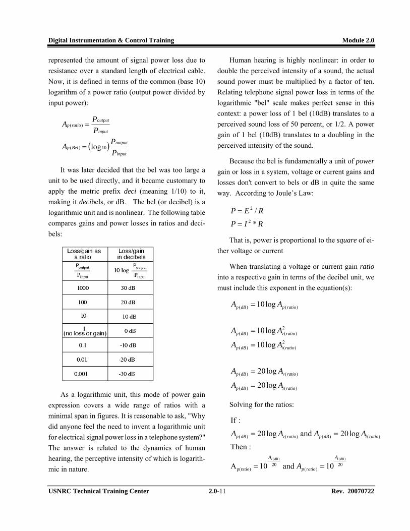
It was later decided that the bel was too large a unit to be used directly, and it became customary to apply the metric prefix deci (meaning 1/10) to it, making it decibels, or dB. The bel (or decibel) is a logarithmic unit and is nonlinear. The following table compares gains and power losses in ratios and deci-bels:
As a logarithmic unit, this mode of power gain expression covers a wide range of ratios with a minimal span in figures. It is reasonable to ask, "Why did anyone feel the need to invent a logarithmic unit for electrical signal power loss in a telephone system?" The answer is related to the dynamics of human hearing, the perceptive intensity of which is logarith-mic in nature.
Human hearing is highly nonlinear: in order to double the perceived intensity of a sound, the actual sound power must be multiplied by a factor of ten. Relating telephone signal power loss in terms of the logarithmic "bel" scale makes perfect sense in this context: a power loss of 1 bel (10dB) translates to a perceived sound loss of 50 percent, or 1/2. A power gain of 1 bel (10dB) translates to a doubling in the perceived intensity of the sound.
Because the bel is fundamentally a unit of power gain or loss in a system, voltage or current gains and losses don't convert to bels or dB in quite the same way. According to Joule’s Law:
RIPREP
*/
2
2
=
=
That is, power is proportional to the square of ei-ther voltage or current
When translating a voltage or current gain ratio into a respective gain in terms of the decibel unit, we must include this exponent in the equation(s):
)()(
)()(
2)()(
2)()(
)()(
log20
log20
log10
log10
log10
ratioidBp
ratiovdBp
ratioidBp
ratiovdBp
ratiopdBp
AA
AA
AA
AA
AA
=
=
=
=
=
Solving for the ratios:
20)(
20p(ratio)
)()()()(
)()(
10 and 10A
:Then
log20 and log20:If
dBidBv A
ratiop
A
ratioidBpratiovdBp
A
AAAA
==
==

Digital Instrumentation & Control Training Module 2.0
USNRC Technical Training Center 2.0-12 Rev. 20070722
2.2.3 “Operational” Amplifiers
The operational amplifier is arguably the most use-ful single device in analog electronic circuitry. With only a handful of external components, it can be made to perform a wide variety of analog signal processing tasks.
For ease of drawing complex circuit diagrams, electronic amplifiers are often symbolized by a simple triangle shape, where the internal components are not individually represented. This symbology is very handy for cases where an amplifier's construction is irrelevant to the greater function of the overall circuit, and it is worthy of familiarization:
The +V and -V connections denote the positive
and negative sides of the DC power supply, respec-tively. The input and output voltage connections are shown as single conductors, because it is assumed that all signal voltages are referenced to a common connection in the circuit called ground. Often, one pole of the DC power supply, either positive or negative, is that ground reference point. A practical amplifier circuit (showing the input voltage source, load resistance, and power supply) might look like this:
Without having to analyze the actual internal de-sign of the amplifier, the above circuit illustrates that its function is to take an input signal (Vin), amplify it, and drive a load resistance (Rload).
Package connections to a typical operational am-plifier are shown below:
The term “DIP” means “Dual In-line Package” to distinguish it from other package types.
Some typical operational amplifiers are shown in the photograph below:
2.2.3.1 The Differential Amplifier
Signifying the amplifier with a triangle symbol makes it easier to study more complex amplifiers and

Digital Instrumentation & Control Training Module 2.0
USNRC Technical Training Center 2.0-13 Rev. 20070722
circuits. One of these more complex amplifier types is called the differential amplifier. Unlike normal amplifiers, which amplify a single input signal (often called single-ended amplifiers), differential amplifiers amplify the voltage difference between two input signals. Using the simplified triangle amplifier symbol, a differential amplifier looks like this:
The two input leads can be seen on the left-hand
side of the triangular amplifier symbol, the output lead on the right-hand side, and the +V and -V power supply leads on top and bottom. As with the other example, all voltages are referenced to the circuit's ground point.
An increasingly positive voltage on the (+) input tends to drive the output voltage more positive, and an increasingly positive voltage on the (-) input tends to drive the output voltage more negative. Likewise, an increasingly negative voltage on the (+) input tends to drive the output negative as well, and an increasingly negative voltage on the (-) input does just the opposite. Because of this relationship between inputs and polarities, the (-) input is commonly referred to as the inverting input and the (+) as the noninverting input.
It is easy to get confused with these polarities and polarity markings (- and +) and not know what the output of the differential amplifier will be. To address this potential confusion, here's a simple rule to remember:
When the polarity of the differential voltage
matches the markings for inverting and noninverting inputs, the output will be positive. When the polarity of the differential voltage clashes with the input markings, the output will be negative.
2.2.3.2 Analog Computing
Long before the advent of digital electronic tech-nology, computers were built to electronically perform calculations by employing voltages and currents to represent numerical quantities. This was especially useful for the simulation of physical processes. A variable voltage, for instance, might represent velocity or force in a physical system. Through the use of resistive voltage dividers and voltage amplifiers, the mathematical operations of division and multiplication could be easily performed on these signals.
The reactive properties of capacitors and inductors lend themselves well to the simulation of variables related by calculus functions. The current through a capacitor is a function of the voltage's rate of change. How is that rate of change designated in calculus as the derivative? If the voltage across a capacitor were made to represent the velocity of an object, the current through the capacitor would represent the force required to accelerate or decelerate that object, the capacitor's capacitance would represent the object's mass:

Digital Instrumentation & Control Training Module 2.0
USNRC Technical Training Center 2.0-14 Rev. 20070722
This analog electronic computation of the calculus derivative function is technically known as differentia-tion, and it is a natural function of a capacitor's current in relation to the voltage applied across it. Note that this circuit requires no "programming" to perform this relatively advanced mathematical function as a digital computer would.
Electronic circuits are easy and inexpensive to cre-ate compared to complex physical systems, so this kind of analog electronic simulation was widely used in the research and development of mechanical systems. For realistic simulation, though, amplifier circuits of high accuracy and easy configurability were needed.
Differential amplifiers with extremely high voltage gains met these requirements of accuracy and con-figurability better than single-ended amplifiers with custom-designed gains. Using simple components connected to the inputs and output of the high-gain differential amplifier, virtually any gain and any function could be obtained from the circuit, overall, without adjusting or modifying the internal circuitry of the amplifier itself. These high-gain differential amplifiers came to be known as operational amplifi-ers, or op-amps, because of their application in analog computers' mathematical operations.
2.2.3.3 Negative Feedback
Practical operational amplifier voltage gains are in the range of 200,000 or more, which makes them almost useless as an analog differential amplifier by themselves. For an op-amp with a voltage gain (AV) of
200,000 and a maximum output voltage swing of +15V/-15V, all it would take is a differential input voltage of 75 µV (microvolts) to drive it to saturation or cutoff!
If we connect the output of an op-amp to its invert-ing input and apply a voltage signal to the noninvert-ing input, we find that the output voltage of the op-amp closely follows that input voltage.
As Vin increases, Vout will increase in accordance
with the differential gain. However, as Vout increases, that output voltage is fed back to the inverting input, thereby acting to decrease the voltage differential between inputs, which acts to bring the output down. For any given voltage input, the op-amp will output a voltage very nearly equal to Vin, but just low enough so that there's enough voltage difference left between Vin and the (-) input to be amplified to generate the output voltage:
))1
(
)()(
+=
=+
−=
−=−=
+
+
+
+
−+
v
vout
outv
out
outv
out
outvout
vout
AAVV
VVA
V
VVA
VVVAVVVAV
The circuit will quickly reach equilibrium, where the output voltage is just the right amount to maintain the right amount of differential, which in turn produces the right amount of output voltage. Taking the op-amp's output voltage and coupling it to the inverting

Digital Instrumentation & Control Training Module 2.0
USNRC Technical Training Center 2.0-15 Rev. 20070722
input is a technique known as negative feedback, and it is the key to having a self-stabilizing system. This stability gives the op-amp the capacity to work in its linear (active) mode, as opposed to merely being saturated fully "on" or "off" with no feedback at all.
2.2.3.4 Feedback Ratio
If a voltage divider is added to the negative feed-back wiring so that only a fraction of the output voltage is fed back to the inverting input instead of the full amount, the output voltage will be a multiple of the input voltage.
By grounding the noninverting input, the negative feedback from the output seeks to hold the inverting input's voltage at 0 volts, as well. For this reason, the inverting input is referred to in this circuit as a virtual ground, being held at ground potential (0 volts) by the feedback, yet not electrically connected to electrical ground. The input voltage is applied to the left-hand end of the voltage divider (R1 = R2 = 1 kΩ again), so the output voltage must swing to -6 volts in order to balance the middle at ground potential (0 volts).
The overall voltage gain of this circuit is calcu-lated by the following formula:
1
2
RR
Av −=
2.2.3.5 Averaging and Summing
The following circuit is called an inverting sum-mer:
With the right-hand sides of the three averaging resistors connected to the virtual ground point of the op-amp's inverting input, the voltage at the virtual ground is held at 0 volts by the op-amp's negative feedback. With all resistor values equal to each other, the currents through each of the three resistors will be proportional to their respective input voltages. Since those three currents will add at the virtual ground node, the algebraic sum of those currents through the feedback resistor will produce a voltage at Vout equal to V1 + V2 + V3 with reversed polarity:
)( 321 VVVVout ++−=
(Up to the supply voltage limit)
2.2.3.6 Differentiation
By introducing electrical reactance into the feed-back loops of op-amp amplifier circuits, the output will respond to changes in the input voltage over time. Drawing their names from their respective calculus functions, the integrator produces a voltage output proportional to the product (multiplication) of the input voltage and time; and the differentiator produces a voltage output proportional to the input voltage's rate of change.
Capacitance is measure of a device’s opposition to changes in voltage. Capacitors oppose voltage change by creating current in the circuit: that is, they either charge or discharge in response to a change in applied voltage. The equation for this is:

Digital Instrumentation & Control Training Module 2.0
USNRC Technical Training Center 2.0-16 Rev. 20070722
The dv/dt fraction is a calculus expression repre-senting the rate of voltage change over time. If the DC supply in the above circuit were steadily increased from a voltage of 15 volts to a voltage of 16 volts over a time span of 1 hour, the current through the capacitor would most likely be very small, because of the very low rate of voltage change (dv/dt = 1 volt / 3600 seconds). However, if we steadily increased the DC supply from 15 volts to 16 volts over a shorter time span of 1 second, the rate of voltage change would be much higher, and thus the charging current would be much higher (dv/dt = 1 volt / 1 second).
The next figure illustrates an op-amp circuit that measures change in voltage by measuring current through a capacitor, and outputs a voltage proportional to that current:
The right-hand side of the capacitor is held to a voltage of 0 volts, due to the "virtual ground" effect. Therefore, current "through" the capacitor is solely due to change in the input voltage. A steady input voltage won't cause a current through C, but a changing input voltage will.
The formula for determining voltage output for the differentiator is as follows:
dtdvRCV in
out −=
Applications for this include rate-of-change indi-cators for process instrumentation. In process control, the derivative function is used to make control deci-sions for maintaining a process at setpoint, by monitor-ing the rate of process change over time and taking action to prevent excessive rates of change, which can lead to an unstable condition. Analog electronic controllers use variations of this circuitry to perform the derivative function.
2.2.3.7 Integration
There are applications in process control where we need the opposite function, called integration in calculus. The op-amp circuit generates an output voltage proportional to the magnitude and duration
Digital Instrumentation & Control Training Module 2.0
USNRC Technical Training Center 2.0-17 Rev. 20070722
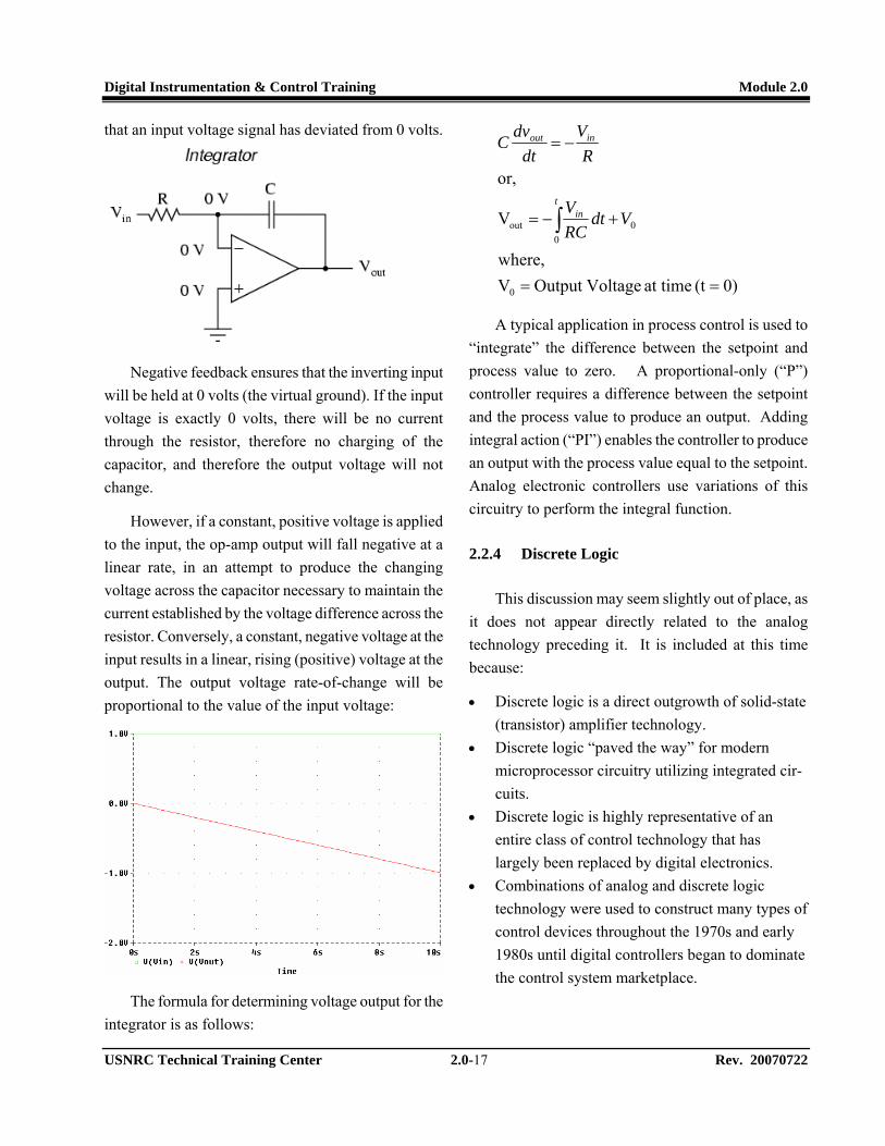
that an input voltage signal has deviated from 0 volts.
Negative feedback ensures that the inverting input will be held at 0 volts (the virtual ground). If the input voltage is exactly 0 volts, there will be no current through the resistor, therefore no charging of the capacitor, and therefore the output voltage will not change.
However, if a constant, positive voltage is applied to the input, the op-amp output will fall negative at a linear rate, in an attempt to produce the changing voltage across the capacitor necessary to maintain the current established by the voltage difference across the resistor. Conversely, a constant, negative voltage at the input results in a linear, rising (positive) voltage at the output. The output voltage rate-of-change will be proportional to the value of the input voltage:
The formula for determining voltage output for the integrator is as follows:
0)(t at time VoltageOutput Vwhere,
V
or,
0
00out
==
+−=
−=
∫t
in
inout
VdtRCV
RV
dtdvC
A typical application in process control is used to “integrate” the difference between the setpoint and process value to zero. A proportional-only (“P”) controller requires a difference between the setpoint and the process value to produce an output. Adding integral action (“PI”) enables the controller to produce an output with the process value equal to the setpoint. Analog electronic controllers use variations of this circuitry to perform the integral function.
2.2.4 Discrete Logic
This discussion may seem slightly out of place, as it does not appear directly related to the analog technology preceding it. It is included at this time because:
• Discrete logic is a direct outgrowth of solid-state (transistor) amplifier technology.
• Discrete logic “paved the way” for modern microprocessor circuitry utilizing integrated cir-cuits.
• Discrete logic is highly representative of an entire class of control technology that has largely been replaced by digital electronics.
• Combinations of analog and discrete logic technology were used to construct many types of control devices throughout the 1970s and early 1980s until digital controllers began to dominate the control system marketplace.

Digital Instrumentation & Control Training Module 2.0
USNRC Technical Training Center 2.0-18 Rev. 20070722
Before the advent of PLCs in the late 1970’s, in-dustrial control was performed either with relays or discrete logic. Relay logic is discussed in the next section.
Discrete logic is the construction of a system de-sign from discrete-logic building blocks: single, dual, quad, and octal gates; counters and timers; latches and registers; etc. There were was no Central Processing Unit (CPU), Read Only Memory (ROM), or Random Access Memory (RAM). Verifying the function and timing of these hardwired multichip assemblages was tedious and time-consuming, and even the slightest design specification change often forced a clean-slate redesign. As tedious as it might have been, use of discrete logic was still a great improvement over its predecessor: discrete components. Discrete component technology is the use of individual resistors, capaci-tors, transistors and diodes to construct a system design. An analog process controller using discrete component technology is shown in Figure 2-2.
2.2.4.1 Single-Input Gate Circuits
Electronic circuits are physical systems that lend themselves well to the representation of binary numbers. When transistors are operated at their bias limits, they may be in one of two different states: either cutoff (no controlled current) or saturation (maximum controlled current). If a transistor circuit is designed to maximize the probability of falling into either one of these states (and not operating in the linear, or active, mode), it can serve as a physical representation of a binary bit. A voltage signal measured at the output of such a circuit may also serve as a representation of a single bit, a low voltage representing a binary "0" and a (relatively) high voltage representing a binary "1." Note the following transistor circuit:
In this circuit, the transistor is in a state of satura-tion due to the applied input voltage (5 volts) through the two-position switch. Because it is saturated, the transistor drops very little voltage between collector and emitter, resulting in an output voltage of (practi-cally) 0 volts. If we were using this circuit to represent binary bits, we would say that the input signal is a binary "1" and that the output signal is a binary "0." Any voltage close to full supply voltage (measured in reference to ground, of course) is considered a "1" (logic level high) and a lack of voltage is considered a "0” (logic level low.
The above circuit is a logic gate, or simply gate, which is a special type of amplifier circuit designed to accept and generate voltage signals corresponding to binary 1's and 0's. Gates are not intended to be used for amplifying analog signals (voltage signals between 0 and full voltage). Multiple gates may be applied to the task of binary number storage (memory circuits) or manipulation (computing circuits), with each gate's output representing one bit of a multi-bit binary number.
The above gate with the single transistor is known as an inverter, or NOT gate, because it outputs the exact opposite digital signal as the input. Gate circuits

Digital Instrumentation & Control Training Module 2.0
USNRC Technical Training Center 2.0-19 Rev. 20070722
are generally represented by symbols rather than by their constituent transistors and resistors. The follow-ing is the symbol for an inverter:
Input and output connections are shown as single wires, the implied reference point for each voltage signal being "ground." In digital gate circuits, ground is almost always the negative connection of a single voltage source (power supply). Dual, or "split," power supplies are seldom used in gate circuitry. Because gate circuits are amplifiers, they require a source of power to operate. As with operational amplifiers, the power supply connections for digital gates are often omitted from the symbol for simplicity's sake. If we were to show all the necessary connections needed for operating this gate, the schematic would look like this:
Power supply conductors are rarely shown in gate circuit schematics, even if the power supply connec-tions at each gate are. Minimizing lines in our schematic, we get this:
A common way to express the particular function of a gate circuit is called a truth table. Truth tables show all combinations of input conditions in terms of logic level states (either "high" or "low," "1" or "0," for each input terminal of the gate), along with the corresponding output logic level, either "high" or "low." For the inverter, or NOT, circuit just illustrated, the truth table is very simple:
A typical discrete logic chip might incorporate 20
- 50 transistors and diode and a comparable number of resistors. By contrast, a modern microprocessor chip incorporates millions of individual transistors and gates. The following photograph illustrates some typical discrete logic integrated circuits:

Digital Instrumentation & Control Training Module 2.0
USNRC Technical Training Center 2.0-20 Rev. 20070722
2.2.4.2 Multiple-Input Gate Circuits
An inverter has only one input; its applications are limited. Adding more inputs increases the range of applications. Some widely-used multiple input gates are discussed below:
AND Gate
One of the easiest multiple-input gates to under-stand is the AND gate. The output of this gate will be "high" (1) if and only if all inputs (first input and the second input and . . .) are "high" (1). If any input(s) are "low" (0), the output is guaranteed to be in a "low" state. An AND gate may have two or more inputs. The truth table for a two-input AND Gate is shown below:
NAND Gate
A variation on the AND gate is called the NAND gate. The word "NAND" is a verbal contraction of the words NOT and AND. A NAND gate behaves the same as an AND gate with a NOT (inverter) gate connected to the output terminal. To symbolize this output signal inversion, the NAND gate symbol has a bubble on the output line. The truth table for a NAND gate is exactly opposite that of an AND gate:

Digital Instrumentation & Control Training Module 2.0
USNRC Technical Training Center 2.0-21 Rev. 20070722
OR Gate
The output of this gate will be "high" (1) if any of the inputs (first input or the second input or . . .) are "high" (1). The output of an OR gate goes "low" (0) if and only if all inputs are "low" (0). A 2-input OR gate truth table is shown below:
NOR Gate
The NOR gate is an OR gate with its output in-verted, just like a NAND gate is an AND gate with an inverted output. The NOR gate truth table is shown below:
Exclusive OR
The Exclusive-OR gate outputs a "high" (1) logic level if the inputs are at different logic levels, either 0 and 1 or 1 and 0. The gate outputs a "low" (0) logic level if the inputs are at the same logic levels. The Exclusive-OR (sometimes called XOR) gate symbol and truth table pattern are shown below:

Digital Instrumentation & Control Training Module 2.0
USNRC Technical Training Center 2.0-22 Rev. 20070722
There are many more kinds of gates than the sim-ple AND, NAND, OR, NOR and XOR discussed above, although it can be argued that nearly all gates are combinations of these basic functions. Also, different technologies exist in which the gate functions are implemented:
• Transistor-Transistor Logic (TTL) (illustrated) • Complementary Metal Oxide Silicon (CMOS) • Diode-Transistor Logic (DTL) • Motorola High-Threshold Logic (MHTL)
The other technologies were developed to address shortcomings in TTL logic. Specifically, CMOS circuits take far less power to operate than TTL. The MHTL logic operates at 15 Vdc rather than 5 Vdc and is inherently more resistant to noise causing unin-tended gate action.
2.3 “Digital” Control Technology
The purpose of this lesson is to provide basic background regarding industrial control technology, from its beginnings in electromechanical relays to its current state in programmable logic controllers. The lesson will discuss “how it works” and continue through “how it is used” in nuclear power plant I&C applications.
2.3.1 Relay Devices
Joseph Henry (1797-1878), invented and used the electromagnetic relay in his laboratory at the College of New Jersey (now Princeton University) laboratory. His low power electromagnet could control a make and break switch in a high-power circuit. Henry believed in the relay’s potential use in control systems, but he was only interested in the science of electricity. The relay was a laboratory trick to entertain students.
Henry also used an electromagnet to create a re-mote signaling device (. The device used an electro-magnet and a bell, and preceded Samuel F. B. Morse’s telegraph. Lawsuits filed at the time indicated that Morse used Henry’s ideas but patented them, making them his own.
A relay is an electromagnetically operated switch. An electric current through a conductor will produce a magnetic field at right angles to the direction of electron flow. If that conductor is wrapped into a coil shape, the magnetic field produced will be oriented along the length of the coil, as shown below:

Digital Instrumentation & Control Training Module 2.0
USNRC Technical Training Center 2.0-23 Rev. 20070722
All other factors being equal, the greater the cur-rent, the greater will be the strength of the magnetic field. The magnetic field produced by a coil of current-carrying wire can be used to exert a mechanical force on any magnetic object, just as we can use a perma-nent magnet to attract magnetic objects, except that this magnet (formed by the coil) can be turned on or off by switching the current on or off through the coil.
A magnetic object placed near the coil will move when the coil is energized. The movable magnetic object is called an armature, and most armatures can be moved with either direct current (DC) or alternating current (AC) energizing the coil. Solenoids can be used to electrically open door latches, open or shut valves, move robotic limbs, and actuate electric switch mechanisms. When the solenoid is used to actuate a set of switch contacts, the device is known as a relay. Construction of a typical armature relay is shown below:
Since Henry’s time, the relay has undergone steady evolution and today's relays are far removed from Henry’s crude and clumsy relays. Solid state construction has replaced the mechanical relay in many applications, especially in AC current control. However, electromechanical relays are still an impor-tant part of modern industrial control technology, because of their ability to handle heavy electrical current economically.
Relays are used to control a large amount of cur-rent and/or voltage with a small electrical signal. The relay coil which produces the magnetic field may consume fractions of a watt of power, while the contacts closed or opened by that magnetic field may be able to conduct hundreds of times that amount of power to a load. In effect, a relay acts as a binary (on or off) amplifier. The relay's ability to control one electrical signal with another enables it to be used in the construction of logic functions. This topic will be covered later. For now, the relay's "amplifying" ability will be explored.
In the next figure, the relay's coil is energized by the low-voltage (12 VDC) source, while the single-pole, single-throw (SPST) contact interrupts the high-voltage (480 VAC) circuit. The current required to energize the relay coil may be orders of magnitude less than the current rating of the contact. Typical relay coil currents are well below 1 amp, while typical contact ratings for industrial relays are at least 10 amps.
One relay coil/armature assembly may be used to actuate more than one set of contacts. Those contacts may be normally-open, normally-closed, or any combination of the two. As with switches, the "nor-mal" state of a relay's contacts is when the coil is de-energized; that is, when the relay is sitting on a shelf in its box, not connected to any circuit.
Relay contacts may be open-air pads of metal al-loy, mercury tubes, or magnetic reeds, just as with other types of switches. The choice of contacts in a
Digital Instrumentation & Control Training Module 2.0
USNRC Technical Training Center 2.0-24 Rev. 20070722
relay depends on the same factors which dictate contact choice in other types of switches. Open-air contacts are the best for high-current applications, but their tendency to corrode and spark may cause prob-lems in some industrial environments. Mercury and reed contacts are sparkless and don't corrode, but they are limited in current-carrying capacity.
A typical industrial control relay is shown in Figure 2-3. A rotary power relay is shown in Figure 2-4. This relay is resistant to vibration and can be qualified to operate used in safety related applications with US West Coast Design Basis and Safe Shutdown Earthquake (DBE and SSE) seismic design criteria. Figure 2-5 illustrates a pneumatic time delay relay. This device uses a pneumatic cylinder that is pressur-ized when the relay is energized. The pressurized cylinder prevents the delayed contacts from operating instantaneously. The pressure bleeds off through a variable orifice. When sufficient pressure is bled off, the contacts operate. These relays are not well-suited for applications where set-point repeatability is important, particularly where seismic qualification is a requirement. Electronic or digital relays offer signifi-cant advantages under these conditions.
Relays provide electrical isolation between coil and contact circuits. That is, the coil circuit and contact circuit(s) are electrically insulated from one another. One circuit may be DC and the other AC or they may be at completely different voltage levels.
In order for a relay to positively operate the arma-ture, there must be a certain minimum amount of current through the coil. This is the "pull in" current. Once the armature is pulled closer to the coil's center, it takes less coil current to hold it. This is the “holding current." The coil current must drop significantly lower than the pull-in current before the armature "drops out" to its shelf position and the contacts resume their normal state. This current level is called the “drop-out” current.
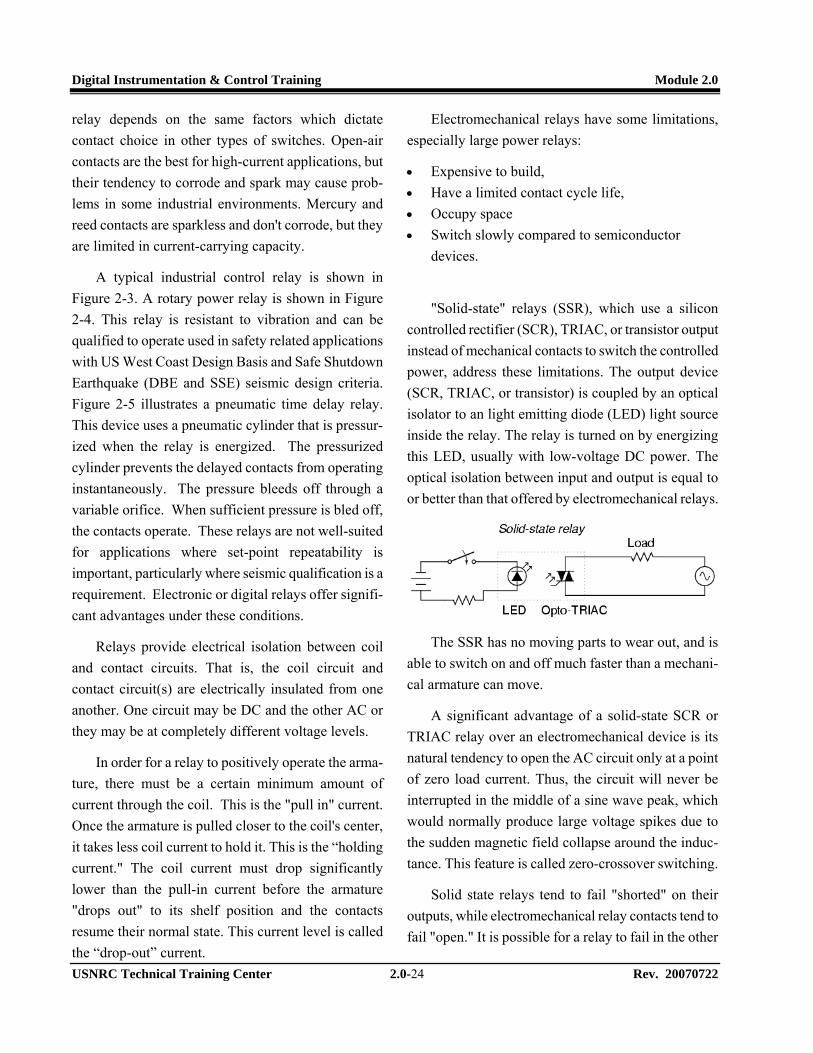
Electromechanical relays have some limitations, especially large power relays:
• Expensive to build, • Have a limited contact cycle life, • Occupy space • Switch slowly compared to semiconductor
devices.
"Solid-state" relays (SSR), which use a silicon controlled rectifier (SCR), TRIAC, or transistor output instead of mechanical contacts to switch the controlled power, address these limitations. The output device (SCR, TRIAC, or transistor) is coupled by an optical isolator to an light emitting diode (LED) light source inside the relay. The relay is turned on by energizing this LED, usually with low-voltage DC power. The optical isolation between input and output is equal to or better than that offered by electromechanical relays.
The SSR has no moving parts to wear out, and is able to switch on and off much faster than a mechani-cal armature can move.
A significant advantage of a solid-state SCR or TRIAC relay over an electromechanical device is its natural tendency to open the AC circuit only at a point of zero load current. Thus, the circuit will never be interrupted in the middle of a sine wave peak, which would normally produce large voltage spikes due to the sudden magnetic field collapse around the induc-tance. This feature is called zero-crossover switching.
Solid state relays tend to fail "shorted" on their outputs, while electromechanical relay contacts tend to fail "open." It is possible for a relay to fail in the other
Digital Instrumentation & Control Training Module 2.0
USNRC Technical Training Center 2.0-25 Rev. 20070722
mode, but these are the most common failures. Because a "fail-open" state is generally considered safer than a "fail-closed" state, electromechanical relays are favored in applications where safety is a primary consideration. [Credit: Lessons In Electric Circuits, 2000-2003 Tony R. Kuphaldt]
As shown later in this lesson, these limitations can be addressed first by different representations of the design, then by using updated technology.
2.3.2 Solid State Logic
Solid state logic was the next step above electro-mechanical relays in the industrial control evolution-ary path. Solid state logic uses the discrete logic devices discussed in Section 2.2.4 to perform control functions.
The Westinghouse Solid State Protection System (SSPS), initially designed in the late 60’s and imple-mented in Westinghouse Pressurized Water Reactor (PWR) plants from that time through the Standard Nuclear Unit Power Plants (SNUPPS) (Wolf Creek, Callaway, Byron, Braidwood, etc.), is an excellent example of this technology. The SSPS was used to perform coincidence logic for Reactor Trip System (RTS) and Nuclear Steam Supply System (NSSS)-related Engineered Safety Function Actuation System (ESFAS) functions. Several of these plants also use a Consolidated Controls Corporation (CCC) solid state logic system for Balance of Plant (BOP)-related ESFAS functions such as Main Steam and Feedwater Isolation, Load Shed, Emergency Load Sequencing, Auxiliary Feedwater Actuation and others. The CCC (Solid State Logic System (SSLS) is a later design and is more advanced.
As regulators, there is a good chance that you will encounter the SSPS in connection with a change to the RTS or ESFAS in a Westinghouse plant.
This section of the lesson will give a brief descrip-tion of the Westinghouse SSPS to illustrate how the system implements its functions using discrete logic components. Of necessity, this forum does not provide sufficient time to provide a detailed descrip-tion. It is important to realize that the complex functions described in this section are all performed by hardwired logic. The logic consists of integrated circuits and discrete components mounted on printed circuit cards. The circuit cards plug into a back plane, which contains all the circuit sockets and the wiring between their pins. The wiring is all done by hand and physically resembles a “rat’s nest.” Changes to the wiring must be done with extreme care, as removing a wire may dislodge other wires. Any change to the SSPS wiring requires a complete test of the entire system, not just the function that was altered or added.
The SSPS equipment provides three functions, as shown in the protection scheme illustrated by Figure 2-6, which also illustrates the plant parameters that provide inputs to the SSPS:
• Automatically provide a reactor trip • Automatically provide a safeguards actuation • Continually provide control board and plant
computer indications of the status of the first two functions.
A simplified diagram of the functions performed by the SSPS and the plant interfaces is provided in Figure 2-7. Physical plant parameters such as tem-perature, pressure, level and flow are sensed by transducers and converted to electrical signals. These signals are sent to the Process Instrumentation racks to be conditioned and compared against setpoints. Nuclear power signals are processed similarly by the Nuclear Instrumentation racks. The outputs of the two instrumentation systems are bistable (on/off) signals that designate if the monitored parameter is within or outside safe operating limits.

Digital Instrumentation & Control Training Module 2.0
USNRC Technical Training Center 2.0-26 Rev. 20070722
The bistable signals are input to the SSSPs via in-put relays (Figure 2-3) that provide isolation between the external protection channels and the SSPS inter-nals. This arrangement is shown in Figure 2-8. The input relay arrangement includes an Inhibit function that allows the logic to be exercised for testing purposes.
The “Brain” of the SSPS is the Universal Logic Card, shown in Figure 2-9. Each universal card contains three different logic circuits. Each logic circuit can perform its functions independently of the other circuits on the same card. The board can be exchanged with any other universal board without any kind of jumpers or special alignments because it is configured by its external connections.
The SSPS trips the reactor by interrupting power to the control rod drive mechanisms (CRDM) using a undervoltage (UV) Driver circuit card (Figure 2-11). During safe operations, the UV driver board will “OR” all the outputs of the universal logic cards that provide reactor trips. The UV Driver Board maintains Reactor Trip Breaker (RTB) undervoltage coils in an energized condition. When a trip is necessary, any trip condition at the card input will cause the card to interrupt the current through the RTB undervoltage coils. When power is interrupted, the breakers trip and the CRDMs release the control rods into the core. This “fail-safe” action ensures the reactor will trip should power fail to the SSPS. An automatic trip also energizes RTB shunt trip coils for backup protection.
The ESF actuation functions of the SSPS operate various plant components that will place the plant in a safe condition if parameters indicate that such action is necessary. Safety feature actuations are the result of energizing slave relays (Figure 2-4) in the output relay cabinet. The slave relays are industrial control relays, some of which have latching arrangements. The relays always energize to cause safeguards action whether the
action is to open or close a contact. This limits occurrence of spurious safeguards actuations.
The slave relays are operated by master relays (Figure 2-3) that are in turn operated by safeguards output driver cards (Figure 2-13). The safeguards driver board is normally used as the current source to drive the master relay. It is also used as a lamp driver and as a signal isolator in other applications. Once set, the SAF Driver board must be reset to deenergize the output device. The circuit used in this card is different from that of the UV driver board. The driver output is 48 Vdc when the driver is turned off and 0 Vdc when turned on. Thus, it acts as a current “sink” for the external device. The UV driver board acts as a current “source.”
Figure 2-15 illustrates the indication portion of the SSPS equipment. The tie line between the control board and plant computer connections allows one status light (or computer input) to be shared by both trains. This tie occurs after the output signals are isolated in the SSPS. The data is multiplexed to keep from having large bundles of cables passing between the SSPS and the displays. Multiplexing allows a large amount of information over a small number of conductors, which reduces and simplifies field wiring. Clock counters in the two trains are synchronized with each other. Each status light or computer output is actuated alternately to produce a steady indication. If one of the multiplexing channels fails, the affected indication will not be activated at the correct time and the indication will “blink” to indicate the failure.
A semi-automatic tester in the system is used to verify operation of the logic circuits that make logic decisions for protection signals that are trips, safe-guards or permissive circuits. The tester sends signals to the circuit being tested via logic test switches. When the tester is in use, the SSPS inputs are inhibited to prevent external conditions from affecting the test. SSPS outputs are blocked to prevent actuation of field
Digital Instrumentation & Control Training Module 2.0
USNRC Technical Training Center 2.0-27 Rev. 20070722
equipment. All possible combinations of trip signals for the circuit under test are applied to the test circuit. The output of the test circuit is fed back to the tester board where it is compared to a reference. The test is stopped and a “BAD” light illuminates to indicate the fault.
[Credit: Westinghouse SSPS I&C Training Man-ual, 1990]
Summary
The Westinghouse SSPS is an example to demon-strate what can be accomplished by using solid-state technology instead of relay technology:
1. The Westinghouse SSPS performs the same protections as its predecessor, the relay logic sys-tem.
2. The SSPS provides far more information regard-ing its operating status and condition than its predecessor, the relay-based protection system.
3. Use of solid-state technology allows far more complex functionality to be implemented in a rea-sonable-sized system than would be possible with relay-based logic. Even if it were possible to im-plement similar functionality in a relay-based sys-tem, it would unlikely be fast enough to perform its safety function. With the enormous number of relays involved and the finite life of relay contacts, the system would be subject to frequent downtime, and the effort to trouble-shoot it would be stagger-ing. In addition, the heat produced would be far in excess of that produced by the SSPS, rendering the relay system’s practicality very bleak.
4. The SSPS multiplexes its status information to interfacing systems, rather than hardwiring, thus simplifying field wiring. The multiplexing func-tion also provides optical isolation to prevent the effects of electrical failures in the nonsafety-
related monitoring equipment from degrading the safety repated functions of the SSPS.
5. Although the indication outputs are multiplexed, they are subject only to the most primitive error checking to determine agreement between the trains. If a discrepancy is found, extensive trou-ble-shooting may still be necessary.
6. The SSPS contains semi-automatic self-test features that systematically test all logic states of the system and alarm discrepancies. Performing equivalent testing with a relay-based system takes far more time and is subject to human error.
7. The testing features minimize the opportunity for human failure causing an inadvertent trip or safe-guards actuation (i.e, inputs inhibited; outputs in test.
8. Modifications to the SSPS, while requiring meticulous care and attention to detail are still more straightforward than with the relay logic sys-tem and much easier to test. If any aspects of the modification and its impact in the self-test system are not properly addressed, the test will fail.
2.3.3 Microprocessor Control (PLC and DCS)
The objective of this lesson is to discuss the two basic building blocks of microprocessor-based control:
• Programmable Logic Controller (PLC) • Distributed Control System (DCS)
The discussion will include their evolution from distinctly separate products to the blurring of function-ality that exists today.
PLC Background

Digital Instrumentation & Control Training Module 2.0
USNRC Technical Training Center 2.0-28 Rev. 20070722
The PLC (i.e. Programmable Logic Controller) was invented to replace the sequential relay circuits for machine control. The PLC works by looking at its inputs and depending upon their state, turning on/off its outputs. The user enters a program that gives the desired results. This concept is illustrated in Figure 2-16. Typical applications for the PLC include:
• Machining • Package • Material handling • Automated assembly • Anything involving sequential operations
A typical modern industrial (non-Nuclear Safety Related) PLC is shown in Figure 2-19.
PLC History
The PLC (Programmable Logic Controller) was invented in the late 1960s to replace sequential relay circuits for machine control. In the automobile industry in particular, annual retooling costs for control systems were increasing rapidly due to the extensive hand wiring involved in building relay panels.
When production requirements changed so did the control system. Relays are mechanical devices with a limited lifetime, which requires strict adherence to maintenance schedules. Troubleshooting is very tedious when so many relays are involved. A typical manufacturing machine control panel included hundreds or thousands of individual relays. Initial wiring, then rewiring, many individual devices, was so complicated and expensive that it was actually cheaper to scrap relay panels and build new ones than to rework the old panels.
The General Motors Hydramatic division devel-oped the following initial PLC specifications in 1968:
• Price competitive with relay controls
• Withstand industrial environment • I/O subassemblies easily replaceable • Collect data and pass it to a central computer • Reusable • Programming easily understood by plant
personnel
Bedford Associates (Bedford, MA) proposed the Modular Digital Controller (MODICON) in 1969 to General Motors. Other companies at the time proposed computer based schemes, one of which was based upon the PDP-8. The other computers were general purpose machines that were not optimized for sequen-tial instruction solving, as was the MODICON. The MODICON 084 brought the world's first PLC into commercial production.
The "new controllers" had to be easily pro-grammed by maintenance and plant engineers, and programming changes had to be performed easily. The answer was to use a programming technique most people were already familiar with and replace me-chanical parts with solid-state ones. The program is necessary because a PLC doesn't understand a sche-matic diagram; it only recognizes code. The PLC is provided with software that translates (compiles) the program into machine code.
The relay-based ladder representation illustrated in Figure 2-17 was commonly understood by plant I&C engineers and was the basis for the first high-level PLC language. In ladder programming, items that will be used are translated into symbols for inputs and outputs. Then they are combined to form the desired function. Figure 2-18 illustrates this concept. There will be more discussion of ladder logic programming in Section 2.4.7.
Communications abilities began to appear in ap-proximately 1973. The first such system was Modi-con's “Modbus.” The PLC could now talk to other

Digital Instrumentation & Control Training Module 2.0
USNRC Technical Training Center 2.0-29 Rev. 20070722
PLCs and they could be far away from the actual machine they were controlling. They could also be used to send and receive varying voltages to allow them to enter the analog world. Unfortunately, the lack of standardization coupled with continually changing technology made PLC communications a nightmare of incompatible protocols and physical networks.
The 90's have seen a gradual reduction in the in-troduction of new protocols, and the modernization of the physical layers of some of the more popular protocols that survived the 1980's. The latest standard (IEC 61131-3, “Programmable Controller Languages”) has tried to merge PLC programming languages under one international standard. Modern PLCs are pro-grammable in ladder logic, function block diagrams, instruction lists, “C” and structured text. Several of these languages will be discussed later.
Personal computers (PC's) are also being used to replace PLCs in some applications. The original company that commissioned the MODICON 084 has switched to PC based control systems
The hardware in modern PLCs allows faster scan times in smaller physical packages. Intelligent I/O interfaces allow distributed processing, where certain compute-intensive applications are executed in dedicated processors at the I/O level, and PID control. Communication highways are becoming standards-based, allowing open communications with other PLCs and Distributed Control Systems (DCS). The communication capability allows the PLCs to support a hierarchical architecture:
• Plant floor level • Automation level • Supervisory level • MIS Level
Software improvements allow use of high level languages such as C++, BASIC and Pascal and even
higher languages such as the IEC 61131-3 suite to be discussed later. Advanced diagnostics identify faults in the controller as well as the controlled machine. Floating point math functions enable complex calcula-tions and improved data handling enables storage, tracking and retrieval of large amounts of data.
Nowadays, PLCs are used in most new "real world" applications. If there is industry present, chances are good that there is a PLC present. Almost any application that needs some type of electrical control has a need for a PLC. The larger the process, the more need there is for a PLC.
For example, assume that when a switch turns on we want to turn a solenoid on for 5 seconds and then turn it off regardless of how long the switch is on for. This can be done with a simple external timer. But what if the process included 10 switches and sole-noids? We would need 10 external timers. What if the process also needed to count how many times the switches individually turned on? We would need a lot of external counters.
DCS History
In the late 1970s, the Distributed Control system began to appear. The key word is "Distributed.” That is, functionality is distributed. The DCS uses multiple processors and has a central database. The controller subsystem performs the control functions, the history node connects the data, the Information Management System (IMS) node gives reports, the operator station provides the Human Machine Interface (HMI), and the engineering station allows engineering changes to be made.
Modern computer-based controllers evolved from traditional instruments and controls. What they look like today depends upon where they came from. The PLC evolved from relay controls, and typically has a limited operator interface. The DCS evolved from

Digital Instrumentation & Control Training Module 2.0
USNRC Technical Training Center 2.0-30 Rev. 20070722
analog controllers. The operator interface was the controller faceplate:
• The process value (PV) is displayed on a calibrated scale.
• The setpoint indicator (SP) is displayed on the same scale.
• There is a controller output (CV) indicator. • There is an option for control element position
indication. • Recorders, indicators and summators provide
additional HMI functions.
The DCS was developed to support the traditional process controller concept shown in Figure 2-20. The process loop is implemented with the following interfaces:
• Process to sensor • Sensor to transmitter • Transmitter to controller • Controller to final control element
o Valve actuator o Variable speed motor drive o Other positioning devices
Original process instruments were located at the process (spatially distributed). They were driven directly by the process (pressure gauges, thermome-ters, level glass etc.) There were no central control rooms because they were not practical with process-driven instrumentation. There were many operators.
Technology was driven by the need to lower costs (fewer operators). Remote transducers enabled the controls to be located remotely from the process into a central control room. Early remote instrumentation was pneumatic, which was inherently slow, and pneumatic tubing was expensive to install. Technol-ogy evolved to overcome limitations, leading to
electronic controls. Process control became central-ized, but wiring was still a large part of project cost.
Distributed control provided a way to reduce these costs by moving control back to the process. An operator interface is provided in the control room, along with history, logging and alarming functions. A “data highway” transmits the information from field units to the control room. This concept is illustrated in Figure 2-21. In the modern DCS, functions are distributed among processors with:
• Operator interface in a central control room • Remote processing units perform local control
and data acquisition • Data archiving, alarming, sequence of events
and other monitoring and supervisory functions are performed in processors separate from the control processors
• A data highway transmits information from the remote units to the control room to reduce wir-ing costs
• Local loops share a local processor • Local processors can communicate data with
each other • There are no direct wire connections from field
instruments to the control room • Analog and digital functions can be associated
in the same local controller • Control algorithms are all digital; there are no
circuit loading issues • New multivariable control strategies are possible
DCS Architecture Evolution
The earliest implementations of closed loop con-trol in digital systems required the power of a main-frame computer, and the DCS evolved from that architecture. Among the first DCS architectures to be developed was the Shared Function Controller, illustrated in Figure 2-22. In this controller, function

Digital Instrumentation & Control Training Module 2.0
USNRC Technical Training Center 2.0-31 Rev. 20070722
processing is distributed; that is, there are individual circuit cards devoted to specific functions:
• Input/Output • Control • Communications
All functions in the controller are shared by all cards in the rack, although the data acquisition cards are frequently located in one rack. Thus, there is a processor rack and an I/O rack. The advantage of this arrangement is that all controllers have the same hardware configuration. It is easy to expand and maintain, and spare parts inventory management is fairly simple. The disadvantage is that a single card failure can disable an entire controller and fail all the control loops implemented in the controller.
To address the single failure issue, the single-loop controller, illustrated in Figure 2-23, was developed. In this design, there are dedicated cards for each control loop. The card is selected for its function:
• Analog loop control • Sequential logic control
Each card has a microprocessor that handles all the functions for that loop:
• Data acquisition • Control • Database
Common functions such as data communications and diagnostics have dedicated cards.
This design reduces the risk of disabling multiple loops due to a single processor failure, but requires more investment in spare parts inventory.
Today, the DCS has evolved to the single control module, illustrated in Figure 2-24. In this design, all
functions are embedded on a single module, incorpo-rating:
• Analog functions • Logic functions • Multiple programming languages • Input & Output • Communications handling
The cards are inserted into a passive I/O bus; that is, all active functions are provided on the control module.
This design enables advanced control strategies, because analog and sequential control functions are provided on the same card, and all system variables are available to all control modules. Although the multifunction cards are more complex and difficult to repair, this design provides inventory benefits. Since modern hardware is very reliable, plants frequently maintain very small inventories and rely on overnight mail for replacements. For critical applications, redundancy provides protection against single failures.
PLC or DCS?
In the early days, there was often much discussion (argument) over whether to use a PLC or a DCS in a given application. Today, PLCs are simply the building blocks of a DCS. Every DCS has to start with some form of control device and most of the time that device is the PLC. When a process being controlled is very large, the PLCs are networked together to form a Distributed Control system. The standalone PLC typically does not have a data history function or an HMI. Its communication capability is used to com-municate information up to higher-level DCS func-tions.
A DCS can be purchased as a complete package, or the user can build his own DCS from commercially available hardware and software. Currently available

Digital Instrumentation & Control Training Module 2.0
USNRC Technical Training Center 2.0-32 Rev. 20070722
software packages are available that provide sophisti-cated HMI and data management functions for applications ranging from a single PLC to an entire control room. These packages typically operate on a personal computer platform running a Microsoft Windows-based 32 bit operating system (NT, 2000 Pro, and XP Pro).
Programming concepts for both PLC and DCS platforms will be discussed in Section 2.6.
2.4 Microprocessor Controller Structure and Components
The purpose of this lesson is to provide an under-standing of the most popular characteristics of micro-processor controllers. The discussion will focus on PLCs, since the fundamental building blocks are the same regardless of the system architecture.
[Credit: NUREG/CR-6090, “The Programmable Logic Controller and its application in Nuclear Reactor Systems”]
Definition
As stated earlier in this lesson, the programmable logic controller (PLC) was originally designed to replace industrial relay-based control systems.
There are very few differences between a PLC and other digital control systems. The definition presented in Section 2.3.3 was so general that it included computers and digital controllers of all types. For the purposes of this lesson, a more focused definition of the PLC is as follows:
A programmable logic controller is a digital operating electronic apparatus that uses a pro-grammable memory for the internal storage of instruction for implementing specific functions such as logic, sequencing, timing, counting, and arithme-tic to control, through digital or analog input/output modules, various type of machines or processes. The digital apparatus must:
• Offer at least one restrictive, higher level, programming language such as ladder logic pro-gramming, Boolean programming, or sequential function charts;
• Contain an operating system that can execute its software in a deterministic manner; and
• Interface primarily to sensors and actuating devices. The programming language must offer as a minimum relay coil and contact, timing, counting, and latch instructions.
Every PLC offers basic relay functions. Most PLCs expand the basic functionality to cover a wide variety of complex functions.
Intelligence
Many features of the computer system may be de-scribed in human terms, such as the CPU being the "brains" of the system. Together, the program and the PLC operating system provide “machine intelligence.”
The PLC machine intelligence is based upon mi-croprocessor electronics. The minimum PLC system consists of a central processing unit (CPU), read only memory (ROM), random access memory (RAM), programming terminal interface electronics, and I/O interfacing electronics. Figure 2-25 illustrates the basic components of a PLC and compares the PLC to the relay-based system it replaces.
2.4.1 Central Processor
The CPU handles all activities of the PLC system. The CPU provides a user programming environment, executes the user program, analyzes incoming data, and responds to the incoming data via control signals to the output modules.
All PLCs contain at least one CPU (typically one electronic printed circuit board) that executes user program instructions and guides all operation within

Digital Instrumentation & Control Training Module 2.0
USNRC Technical Training Center 2.0-33 Rev. 20070722
the PLC. In more complex systems, the CPU will communicate with and control the operation of other subsystems within the PLC. Other subsystems may be arithmetic logic units, floating point processors or co-processors, but the CPU has central control over the entire PLC system. The subsystems may contain microprocessors, but their control is limited to the subsystem.
2.4.2 Memory
The two basic types of memory available to the CPU are:
• Read Only Memory (ROM) • Random Access Memory (RAM)
The operating system and programming language interpreter commands are usually stored in ROM, while the user program and the input/output data are stored in RAM. The CPU cannot change ROM memory, while it can change RAM memory as needed. In a typical application, the system will download the contents of the ROM to RAM at initialization because access time for RAM is usually much faster than ROM.
ROM memory is programmed at the time of manu-facture, and may only be changed by replacing the ROM hardware. Programmable ROM may be changed after manufacture. They are erased by high voltage (25-50 Vdc) or ultraviolet light, and can be re-programmed after erasure. These types of ROM are usually removed from the circuit in order to be reprogrammed. Electrically alterable read-only memory (EAROM) may be erased and re-programmed while in the circuit.
The CPU uses its RAM to store the constantly changing input/output data, intermediate calculations, user programs, and various data that must change
during the operation of the PLC. Two types of RAM are available, non-volatile and volatile. Non-volatile memory holds its memory values even if power is removed. Volatile RAM requires battery back-up power to sustain memory through a power outage, a key maintenance issue. The PLC system should have a means to indicate low back-up battery power as an external alarm.
2.4.3 Power Supply
The power supplies include all sources of power necessary to properly operate the PLC system. The typical primary power supply converts 120 Vac or 240 Vac into the low-voltage DC power necessary for operation of the processor and I/O modules. The primary power supplies may be located on each module (processor or I/O), contained in the mounting rack, or the processor module may supply power to the I/O modules. Most manufacturers design the mounting rack such that each rack has one power supply, making this one power supply a single-point failure. If the power supply malfunctions, the entire PLC system fails. A more reliable scheme provides redundant power supplies.
Both linear and switching power supplies are used in PLC power supply designs. Linear power supplies use transformers, rectifiers, and various filtering and detection circuits to transform high-voltage AC power into low-level DC power. The switching power supply is a newer design that is physically smaller, has a higher signal conversion efficiency and produces less heat. However, the switching power supply responds more slowly to electrical transients and produces more noise, which shows up as low-voltage ripple on the DC output lines and in EMI. The switching power supply can also impose harmonic distortion (particu-

Digital Instrumentation & Control Training Module 2.0
USNRC Technical Training Center 2.0-34 Rev. 20070722
larly third harmonic) on the input ac supply, which can adversely affect the operation of static inverters.
Features that should be designed into both types of power supplies include input filters, output filters, short circuit and overload protection, overvoltage and reverse-voltage protection, and incoming line monitor-ing. Input filters reduce incoming electrical transients, while output filters stabilize the power supply's low-voltage DC output and reduce unwanted noise. Short-circuit-overload circuits protect the power supply from destroying itself during abnormal current conditions. Likewise, over-voltage and reverse-voltage protection circuits protect against abnormal voltage conditions. Incoming line monitoring can detect power outages and give warning to the PLC processor, allowing the processor to shut down the system in an orderly fashion.
Batteries are used to back up volatile RAM mem-ory or the real-time clock system. Manufacturers use primary and secondary battery systems. Primary batteries cannot be charged, while secondary batteries are rechargeable. The PLC system should be capable of producing a local and a remote alarm for low-battery status. A low-battery status alarm at a remote terminal can reduce the probability of one inexpensive battery shutting down the entire plant.
Primary battery types include carbon zinc, alka-line, and lithium. All need replacement about once a year. Secondary batteries require a recharging circuit. Their replacement period is much longer than primary battery types and depends on battery usage. In the past, nickel-cadmium battery systems were used widely for secondary battery systems. Nickel metal hydride (NiMH) and lithium ion (Lion) secondary batteries are now common.
2.4.4 Input Structure
PLC input modules are either discrete or analog. The input module receives signals from the field input devices, conditions those signals, and isolates them from the PLC processor. The standard PLC input structure consists of six basic blocks, as shown in Figure 2-26.
1. Field Input devices
Typical discrete inputs are contacts, limit switches, pushbuttons, and pressure/flow/temperature switches. Analog inputs cover a wide range of applications and functionality. Typical analog devices are pres-sure/flow/temperature transducers, motor control signals, vibration transducer, strain gage, load cell, and other transducers producing electrical outputs.
2. I/O Terminations
I/O module terminations provide the interconnec-tion between the field input devices and the PLC system. Termination designs vary greatly. Some are fixed to the module (Figure 2-19), some can be quickly disconnected, and others are fixed to the support structure of the I/O module (Figure 2-52). If the terminations can be disconnected from the module or are part of the structure, I/O modules can be removed and replaced without rewiring.
3. Signal Conditioning
Signal conditioning varies depending on the manu-facturer, the system architecture, and the type of signal conversion required.
Discrete input conversion is relatively simple, while analog input conversions are more complex. Some common types of conditioning circuits are rectifiers, resistors, resistor/capacitor/inductor net-works, and analog conversion. Rectifiers convert incoming AC signals to the desired processor levels. Resistor networks provide DC level attenuation. Resistor/capacitor/inductor networks remove un-

Digital Instrumentation & Control Training Module 2.0
USNRC Technical Training Center 2.0-35 Rev. 20070722
wanted noise spikes and reduce false input triggering due to field device contact bounce.
Analog conversion comes in two forms, counters or A/D converters. Counters transform pulse train waveforms into a binary number representing the number of pulses per unit time. A/D converters convert a varying DC level to a binary representation of the level.
4. Isolation
Isolation circuits mechanically and electrically isolate the field device signals from the PLC processor signals. Isolation limits the possibility of noise and voltage spikes damaging the sensitive processor electronics. Three isolation techniques are employed:
• Opto-isolation – the most common • Transformer isolation – most common before
development of opto-isolation. Transformers are still used in a limited number of designs.
• Reed relays provide a third technique for isolation. A major drawback to reed relays is the limited mechanical life. In the best reed relays the contacts wear out within tens of thousands of cycles. Reed relays are not recommended for applications involving intense cycling.
The isolation surge voltage, Viso, is an important characteristic for isolation devices used to prevent adverse affects on safety-related circuits caused by faults in non-safety circuits. Viso is a measure of the internal dielectric breakdown rating of the opto-electronic device, not necessarily the I/O module. This voltage is placed across the device as shown below:
A typical Viso specification is about 1500 Vdc for 60 seconds and 1500 Vac, 47 to 70 Hz, for 60 seconds.
5. PLC Interface/Multiplexing
This portion of the I/O module gathers all incom-ing conditioned field device signals, and transmits them to the processor as requested. Control signals are produced by this unit and the PLC processor to coordinate the transfer of data. These signals may include clock, reset, enable, module address, hand-shaking, error-handling signals or data.
Some manufacturers provide watchdog timers in this part of the I/O module. The watchdog timer must be reset periodically by the PLC processor. If the processor does not communicate to the I/O within a specified time period, the watchdog timer expires and the outputs are to a predetermined “safe” state as long as the PLC is supplied with power. A system-level alarm is usually generated as well.
6. Indicators
Indicators assist the user in troubleshooting the system and aid in verifying the integrity of the field wiring, the module operation, and the module status. LEDs, neon lamps, and incandescent lamps are all used as indicators, with LEDs being the most common. The indicators may be located and powered on the field device side or the CPU side of the module.
2.4.5 Output Structure

Digital Instrumentation & Control Training Module 2.0
USNRC Technical Training Center 2.0-36 Rev. 20070722
Output modules are either discrete or analog. Typically, discrete outputs control relay coils, valve solenoids, motor starters, panel indicators, and alarms. Analog outputs cover a wide range of applications and functionality. Typical devices controlled by analog outputs are control valves, motor control signals, analog indicators and recorders and other applications needing analog electrical signals. The output module receives signals from the PLC processor, converts and isolates those signals, and controls the field output devices. The standard PLC output structure consists of seven basic blocks as shown in Figure 2-27.
1. PLC Interface/Multiplex Electronics
The PLC interface/multiplex electronics gathers the PLC processor signals, decodes the address, and passes them to the appropriate output destination point. Control signals are provided by the PLC processor to enable this block to function correctly. Typical control signals are clock pulses, reset, enable signals, addressing data, and error handling data. The interface/multiplex electronics sends reply and status data back to the PLC processor.
2. Signal Latching
The signal latching circuitry contains electronic latches such as flip-flops to hold the latest data received from the CPU via the multiplexing electron-ics. The data is held until the next update of output data. The PLC processor ensures that the latch block is updated within a specified time period.
3. Isolation
The isolation circuitry for output modules is iden-tical in design to the input module isolation circuits.
4. Signal Conversion
The signal conversion circuitry converts the latched signals to the proper signal level for the field output device. The signal conversion circuitry is on the
field side of the isolation circuitry. Power for the signal conversion circuitry must come from the field side to isolate the PLC and output module electronics from noisy field devices. The signal conversion circuitry will contain a power switch, typically a triac, reed relay, transistor, or digital-to-analog converter depending on the application. Good practice provides a circuit protector in series with each power switch. The best designs have on-board circuit protectors such as fuses for each output point.
5. I/O Module Terminations
The output module terminations are identical to the input module terminations. Typically, the termina-tions are locked down in some way, such as screw termination blocks. The wire ends may be terminated with lugs to assure a positive, tight contact that will not loosen over time. Good designs provide the capability to remove and replace the I/O module without rewiring by fixing the module terminations to the rack instead of the I/O module. See Figure 2-19 and Figure 2-52 to contrast field termination designs.
6. Field Output Devices
The field output devices provide the muscle to control the process, and the visual and audio informa-tion that expresses the process state. These devices convert the PLC control signals into process changes or status. Process changes are accomplished through control of valves, motors, relays, etc. Process status is presented through graphical displays, horns, lights, and other devices.
7. Indicators
Indicators aid the user in troubleshooting. The out-put module indicators may be powered from the field side or the processor side of isolation circuitry. Some output modules have an additional indicator to detect a blown fuse. The fuse is located on the field side of the isolation circuitry and the indicator connects in parallel
Digital Instrumentation & Control Training Module 2.0
USNRC Technical Training Center 2.0-37 Rev. 20070722
to the fuse. When the fuse blows, the indicator lights up.
2.4.6 Peripheral Devices
Peripherals aid in programming, storing data, printing, emulation, simulation, or other functions the user may need or want.
2.4.6.1 Programming/Maintenance Terminals
The single most important peripheral is the pro-gramming terminal. The programming terminal accepts the program commands of the user, converts them into machine-readable code for the PLC proces-sor, and allocates the machine code into the appropri-ate memory locations within the PLC processor. Once the code is developed, it is downloaded to the PLC.
Programming Modes
As in all computer systems, various modes of op-eration exist in the programming terminal. The two most common modes are on line and off line. On line and off line refer to the mode into which the PLC processor is placed by the programming terminal.
On line programming allows the user to add, change, or delete the PLC program or data while the PLC is running. The user must be careful not to cause undesirable actions in the control process. Most terminals let the user monitor the new program changes before downloading them to the PLC proces-sor to allow the user to monitor the changes and ensure correct process control will result. On line program-ming changes should not be made after start up unless the on line mode is deemed absolutely necessary, and then only with the appropriate Verification and Validation (V&V). Online programming is of value when troubleshooting the system.
Off line programming is more common. The user enters the program into the programming terminal with no effect to the PLC processor. When completed, the user may download the program into the PLC proces-sor. In the off line program mode, the PLC processor will stop scanning and drive outputs to a predeter-mined safe state. Care must be taken to place the controlled equipment in a safe condition before going off line.
Forcing Commands
The “Forcing” command holds an input or output at a desired state. After forced values have been entered for the selected values, a second command is required to enable the forced values, which writes the orced values of the selected I/O points into the appropriate PLC I/O image table. When values have been forced or enabled, other commands are usually required to disable forced inputs, remove the forced value and return the I/O point to normal operation.
Forcing is useful in debugging the program and verifying proper operation of outputs and their connected equipment during testing or maintenance, but can cause equipment damage or personnel injury if not used under proper administrative or procedural controls. Forcing can cause real process events (valves to close/open, motors to start/stop, etc.) to occur. Important equipment such as safety interlocks and motor seal-in contacts can be bypassed. Similarly, equipment may operate unexpectedly when the forces are removed.
Most PLC systems provide alarms to indicate that values have been forced and that the forced values have been enabled.

Digital Instrumentation & Control Training Module 2.0
USNRC Technical Training Center 2.0-38 Rev. 20070722
2.4.6.2 Other Peripherals
Tape drives, floppy drives, hard-disk drives, and solid state memory cards are all available to provide storage of program and PLC system status. Printers of all sorts and varieties are available.
2.4.7 Run-time Operation and Response Time
Run-time mode specifies the period of time in which the PLC executes the user's program. It is a sequential process with five major steps:
1. All input modules are scanned and checked for address or data errors and diagnostics.
2. The input image table in the PLC RAM is updated.
3. The CPU executes the user's logic program using the input image table data as needed in each step.
4. The output image table is updated. 5. The PLC outputs the results to the output
modules. The execution of all five steps is called a scan cy-
cle. The entire user program is executed in one scan cycle. The PLC repeats the scan cycle until it is stopped by the user or shut down. Figure 2-28 outlines the Run-Time steps.
The input data table is not updated until the next scan. Therefore, program operations that are used in subsequent operations may take more than one scan to complete the operation and produce the final output. This determines the response time of the PLC and is illustrated in Figure 2-29.
The PLC only “sees” inputs when it is looking. If a true input clears before the input data table is updated, the PLC will not “see” it until the next scan. Similarly, if the true input clears after the input data table is updated, the PLC will not respond to the cleared signal until the next scan. Outputs are turned
on at the end of the output phase. These effects determine the maximum response time of the PLC, as shown in Figure 2-30; that is, the maximum response time is:
2*Scan time –input delay
where the input delay is defined as the time between the start of scan and the input event.
During program execution, different controller functions are performed by different modules. The time required to execute each module can vary depending on the number of processing steps con-tained in each module. During the scan, the program goes through all steps and starts over. Some pro-gramming languages allow the program to be inter-rupted. Interruptible programs are not desirable, because interruptions can take place inadvertently or as a result of process chanages. As a result, calculation of the total scan time for the program, including all its modules, may not be straightforward.
As shown in Figure 2-31, there are two methods of addressing varying resource requirements:
• Fixed Time Slots: In this method, all functions execute within the same time length in a fixed number of time slots. All elements in the pro-gram must fit into the available slots. Calculat-ing scan time is simple – How many slots are occupied? Because some operations take less time than others, some processing time is wasted
• Variable Time Slots: In this method, each function uses only the time needed for execu-tion. The irregular times are added together to determine the scan time. There is no wasted processing time, because the functions are com-piled and a copy of the function is placed in the program each time it is used.

Digital Instrumentation & Control Training Module 2.0
USNRC Technical Training Center 2.0-39 Rev. 20070722
This method was developed originally because early programs tended to be resource intensive. Today, this is no longer a problem with modern, high-speed processors and fast, inexpensive memory. Variable scan time is not desirable for safety-related applications if program behavior is not deterministic; that is, the execution sequence can change through branches or interrrupts as conditions change external to the application program. If the execution cycle cannot be influenced by external events, it is determi-nistic and acceptable for use in nuclear plant safety syatems, provided other requirements for such safety-related usage are met..
2.5 Digital Communications
The purpose of this lesson is to understand the ba-sics of digital communication, its advantages, disad-vantages, and practical considerations
The lesson will discuss how one digital device communicates information to and from other devices, and how the structures discussed above are tied together to form a control system.
2.5.1 Introduction
It is often necessary to have one device communi-cate digital information to and from other devices. Digital information is far more resistant to transmitted and interpreted errors than information transmitted in an analog medium. However, digital communication has its own unique pitfalls, and there are multitudes of different and incompatible ways in which it can be sent.
Remote Analog Monitoring
Task is to remotely monitor the level in a water storage tank. Measuring the tank level is easy, with many different types of sensors available. For this
example, we will choose an analog level transmitter with a 4-20 mA output:
The transmitter outputs 4 mA at zero level and 20 mA at 100% level. The simplest solution is to send the analog signal to the remote location on a pair of copper wires. In most cases, this is a good solution. However, this lesson is about digital communications, so we will explore methods of transmitting the information digitally.
The analog system has limitations. If the tank is at 50% level, the transmitter output will be 12 mA. However, if there is noise on the electrical signal, the noise will be interpreted as a change in the water level. With no noise, the signal would look like this:
If the analog signal wiring were arranged too closely to wires carrying 60 Hz ac power, inductive and capacitive coupling may create a false noise signal into the dc circuit. The noise coupling would be small, but could upset the measurement:

Digital Instrumentation & Control Training Module 2.0
USNRC Technical Training Center 2.0-40 Rev. 20070722
That is, any electrical noise introduced into an analog measurement system will be interpreted as changes in the measured signal.
Remote Digital Monitoring
The analog level transmitter can be replaced with a crude set of level switches located at different heights in the tank:
The switches are wired so that each switch closes and lights a lamp when the water level rises above its level. A person looking at a control panel would see a 5-lamp representation of the tank level. Each lamp is 100% digital; either 100% ON or 100% OFF. Electri-cal noise interference from other circuits along the signal run would have much less effect on the accu-racy of the indication. It would require extreme interference to cause an OFF signal to be interpreted as ON and vice versa. In this case, however, resolution is limited by the small number of switches.
Increasing the number of switches improves reso-lution. But it also increases the number of wires. In
the next picture, there are sixteen (16) switches. Normally, this would require seventeen (17) wires. A hardwired encoder will generate a binary number that represents the same information:
Only four (4) wires, plus any ground and power wires, are required to transmit the same information. This illustrates the concept of multiplexing.
The customer might not be happy with 1/16 tank height resolution. Adding more switches would improve resolution, but would get cumbersome very quickly. A better solution would be to go back to the 4-20 mA analog transmitter and electronically convert the analog signal to a binary signal with many more bits than would be practical with switches. The electrical noise that causes trouble with the analog signal transmission occurs along the circuit route. If the A/D conversion takes place at the tank, where the environment is electrically “clean”, the noise problem is minimized. There are a number of schemes for converting analog data to binary words. For this lesson, we will concentrate on the digital communica-tion.
The type of digital information being sent from the tank to the monitoring panel is parallel digital data. Each binary bit is sent along a dedicated wire. All the bits arrive at their destination at the same time. If there are many bits in the digital word, many wires are required to transmit the data. The wiring can be
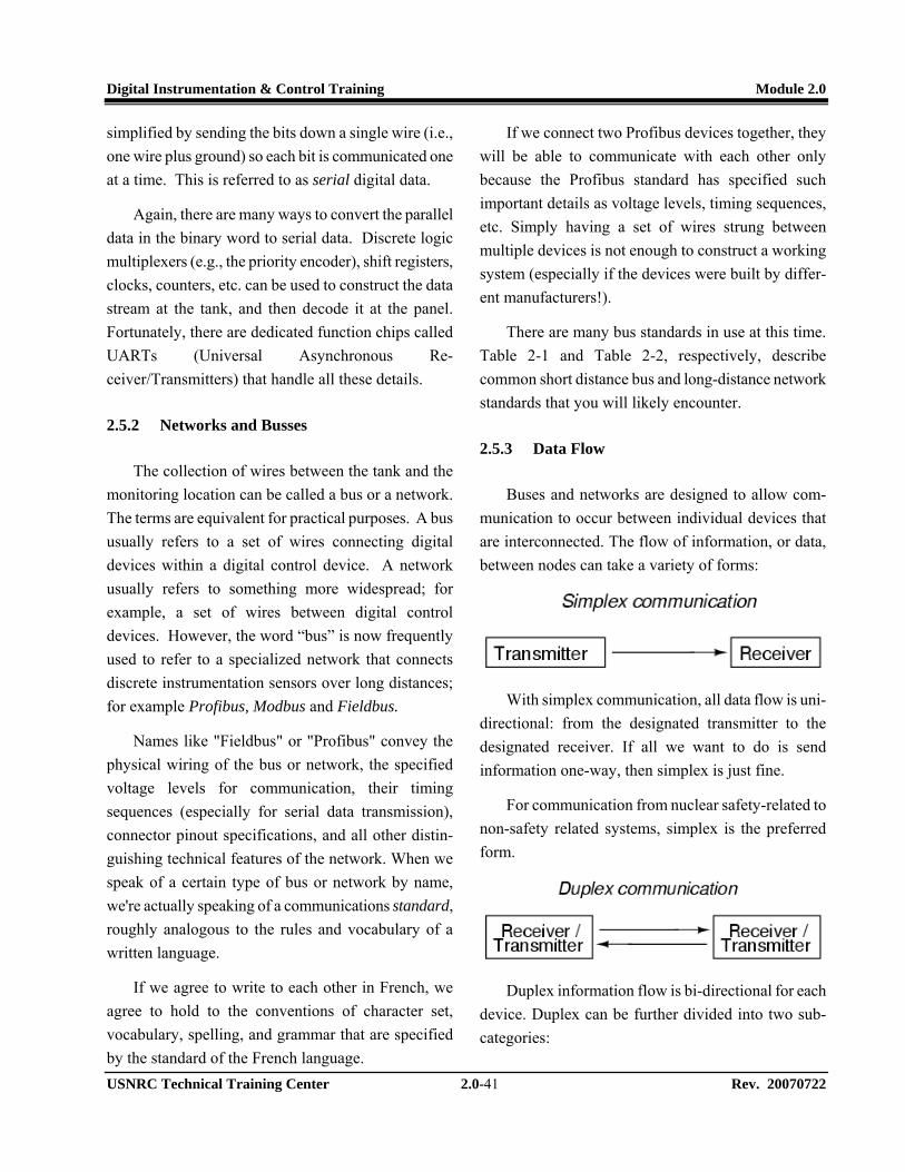
Digital Instrumentation & Control Training Module 2.0
USNRC Technical Training Center 2.0-41 Rev. 20070722
simplified by sending the bits down a single wire (i.e., one wire plus ground) so each bit is communicated one at a time. This is referred to as serial digital data.
Again, there are many ways to convert the parallel data in the binary word to serial data. Discrete logic multiplexers (e.g., the priority encoder), shift registers, clocks, counters, etc. can be used to construct the data stream at the tank, and then decode it at the panel. Fortunately, there are dedicated function chips called UARTs (Universal Asynchronous Re-ceiver/Transmitters) that handle all these details.
2.5.2 Networks and Busses
The collection of wires between the tank and the monitoring location can be called a bus or a network. The terms are equivalent for practical purposes. A bus usually refers to a set of wires connecting digital devices within a digital control device. A network usually refers to something more widespread; for example, a set of wires between digital control devices. However, the word “bus” is now frequently used to refer to a specialized network that connects discrete instrumentation sensors over long distances; for example Profibus, Modbus and Fieldbus.
Names like "Fieldbus" or "Profibus" convey the physical wiring of the bus or network, the specified voltage levels for communication, their timing sequences (especially for serial data transmission), connector pinout specifications, and all other distin-guishing technical features of the network. When we speak of a certain type of bus or network by name, we're actually speaking of a communications standard, roughly analogous to the rules and vocabulary of a written language.
If we agree to write to each other in French, we agree to hold to the conventions of character set, vocabulary, spelling, and grammar that are specified by the standard of the French language.
If we connect two Profibus devices together, they will be able to communicate with each other only because the Profibus standard has specified such important details as voltage levels, timing sequences, etc. Simply having a set of wires strung between multiple devices is not enough to construct a working system (especially if the devices were built by differ-ent manufacturers!).
There are many bus standards in use at this time. Table 2-1 and Table 2-2, respectively, describe common short distance bus and long-distance network standards that you will likely encounter.
2.5.3 Data Flow
Buses and networks are designed to allow com-munication to occur between individual devices that are interconnected. The flow of information, or data, between nodes can take a variety of forms:
With simplex communication, all data flow is uni-directional: from the designated transmitter to the designated receiver. If all we want to do is send information one-way, then simplex is just fine.
For communication from nuclear safety-related to non-safety related systems, simplex is the preferred form.
Duplex information flow is bi-directional for each device. Duplex can be further divided into two sub-categories:

Digital Instrumentation & Control Training Module 2.0
USNRC Technical Training Center 2.0-42 Rev. 20070722
Half-duplex communication is analogous to two tin cans on the ends of a single taut string: Either can be used to transmit or receive, but not at the same time.
Full-duplex communication is more like a true telephone, where two people can talk at the same time and hear one another simultaneously, the mouthpiece of one phone transmitting to the earpiece of the other, and visa-versa.
Full-duplex is often facilitated through the use of two separate channels or networks, with an individual set of wires for each direction of communication.
2.5.4 Electrical Signal Types
Transmitting serial data creates challenges in de-livering information accurately and at an adequate speed. With parallel data, all the data is received at once. With serial data, it is sent one bit at a time, and all bits must be sent in sequence. With an eight bit word, the data rate is necessarily eight times faster if only a single bit is changing.
The data being transmitted is a square wave. A square wave is mathematically equivalent to an infinite series of sine waves of diminishing amplitude and increasing frequency. As the information travels down a transmission line, the high frequencies are attenuated
and the square wave isn’t square anymore. Electrical interference can corrupt the data and cause errors.
Bandwidth is the practical frequency limit of the network. The standard measure of bandwidth is bits per second (bps).
There are two common methods of transmitting the electrical signal:
• Ground Referenced Method
• Differential Voltage Method
The ground-referenced method is the worst case for high frequency square wave voltage attenuation. The method works well for short distances, where inductive and capacitive effects can be controlled. Over long distances, it becomes problematic quickly.
In the differential-voltage method, each bit is rep-resented as the difference between a pair of wires that is isolated from ground. The capacitance between the isolated wires can be controlled much more easily than with a single wire. Capacitive coupling to ground is balanced between the two wires and has little effect.
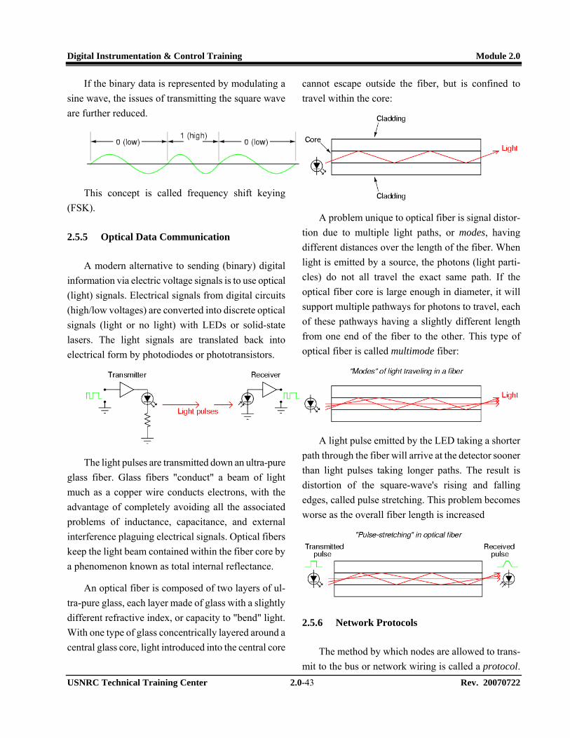
Digital Instrumentation & Control Training Module 2.0
USNRC Technical Training Center 2.0-43 Rev. 20070722
If the binary data is represented by modulating a sine wave, the issues of transmitting the square wave are further reduced.
This concept is called frequency shift keying (FSK).
2.5.5 Optical Data Communication
A modern alternative to sending (binary) digital information via electric voltage signals is to use optical (light) signals. Electrical signals from digital circuits (high/low voltages) are converted into discrete optical signals (light or no light) with LEDs or solid-state lasers. The light signals are translated back into electrical form by photodiodes or phototransistors.
The light pulses are transmitted down an ultra-pure glass fiber. Glass fibers "conduct" a beam of light much as a copper wire conducts electrons, with the advantage of completely avoiding all the associated problems of inductance, capacitance, and external interference plaguing electrical signals. Optical fibers keep the light beam contained within the fiber core by a phenomenon known as total internal reflectance.
An optical fiber is composed of two layers of ul-tra-pure glass, each layer made of glass with a slightly different refractive index, or capacity to "bend" light. With one type of glass concentrically layered around a central glass core, light introduced into the central core
cannot escape outside the fiber, but is confined to travel within the core:
A problem unique to optical fiber is signal distor-tion due to multiple light paths, or modes, having different distances over the length of the fiber. When light is emitted by a source, the photons (light parti-cles) do not all travel the exact same path. If the optical fiber core is large enough in diameter, it will support multiple pathways for photons to travel, each of these pathways having a slightly different length from one end of the fiber to the other. This type of optical fiber is called multimode fiber:
A light pulse emitted by the LED taking a shorter path through the fiber will arrive at the detector sooner than light pulses taking longer paths. The result is distortion of the square-wave's rising and falling edges, called pulse stretching. This problem becomes worse as the overall fiber length is increased
2.5.6 Network Protocols
The method by which nodes are allowed to trans-mit to the bus or network wiring is called a protocol.

Digital Instrumentation & Control Training Module 2.0
USNRC Technical Training Center 2.0-44 Rev. 20070722
There are many different protocols for arbitrating the use of a common network between multiple nodes. This lesson will only cover a few of the most common methods to assist you understand why some work better for some purposes than others. A specific protocol is usually associated with a standardized type of network.
Single Transmitting Node
In this protocol, there is only one transmitter. The other nodes are receivers.
Multiple Transmitting Nodes
Transmissions must be controlled so they don’t conflict with one another. Nodes have the ability to refrain from talking unless the network is silent. This is called Carrier Sense Multiple Access (CSMA). If two or nodes try to talk at the same time, the result is a collision. Different CSMA variations respond to collisions in different ways. With Ethernet, nodes that collide simply reset themselves with a random delay timer circuit, and the first one to finish its time delay tries to talk again.
A different strategy is the Master/Slave protocol, where a single master device allots time slots for all the other nodes on the network to transmit, and schedules these time slots so that multiple nodes cannot collide. The master device addresses each node by name, one at a time, letting that node talk for a certain amount of time. When it is finished, the master addresses the next node, and so on.
Another strategy is the Token-Passing protocol, where each node gets a turn to talk (one at a time), and then grants permission for the next node to talk when it's done. Permission to talk is passed around from node to node as each one hands off the "token" to the next in sequential order. Although token-passing protocol is often associated with ring-topology
networks, it is not restricted to any topology in particular.
2.5.7 Network Topology
Network topology is, literally, the shape of the network.
If there are only two digital devices in the net-work, the network is “point-to-point:”
The line between the devices can be a twisted pair of wires, a coaxial or fiber optic cable, or a radio link.
If more devices (nodes) are needed, there are more options:
Bus (peer – peer) topology is simple to install and maintain. Nodes can be easily added or removed with minimal wiring changes. However, the one bus network must handle all communication signals from all nodes. Only one device can communicate at a time. A break in the bus wiring can cause nodes to become isolated. A practical application for peer – peer networking is gathering data from remote devices, as shown in Figure 2-32.

Digital Instrumentation & Control Training Module 2.0
USNRC Technical Training Center 2.0-45 Rev. 20070722
With “gateways” located at branching points in the network, data flow can be restricted between nodes, allowing for private communication between specific groups of nodes. This addresses some of the speed and security issues of the simple bus topology. However, those branches can be easily cut off from the rest of the "star" network if one of the gateways were to fail. This topology can also be implemented with "switches" to connect individual nodes to a larger network on demand. A disadvantage of this topology is that all communications must go through the hub or “master.”
This topology provides the best reliability with the least amount of wiring. Since each node has two connection points to the ring, a single break in any part of the ring doesn't affect the integrity of the network. The devices must be designed with this topology in mind. Ring networks are broadcast by nature.
Two or more ring topologies may be combined to provide redundancy. Most industrial control network schemes provide this capability.
2.5.8 Practical Considerations
A principal consideration for industrial control networks, where the monitoring and control of real-life processes must often occur quickly and at set times, is the guaranteed maximum communication time from one node to another.
The ability for a network to guarantee data "throughput" is called determinism. A deterministic network has a guaranteed maximum time delay for data transfer from node to node, whereas a non-deterministic network does not. The preeminent example of a non-deterministic network is Ethernet, where the nodes rely on random time-delay circuits to reset and re-attempt transmission after a collision. Since a node's transmission of data can be delayed indefinitely from a long series of re-sets and re-tries after repeated collisions, there is no guarantee that its data will ever get sent out to the network. Realistically, the odds that such a thing would happen are so great that it is of little practical concern in a lightly-loaded network.
Network fault tolerance is another important con-sideration. How susceptible is a particular network's signaling, topology, and/or protocol to failures? A Master/Slave network, while extremely deterministic (a good thing for critical controls), is entirely depend-ent upon the master node to keep everything going (a bad thing for critical controls). If the master node fails for any reason, none of the other nodes will be able to transmit any data at all, because they'll never receive their allotted time slot permissions to do so, and the whole system will fail.
[Credit: Lessons In Electric Circuits, 2000-2003 Tony R. Kuphaldt]
2.6 Digital Controller Programming

Digital Instrumentation & Control Training Module 2.0
USNRC Technical Training Center 2.0-46 Rev. 20070722
The purpose of this lesson is to review the evolu-tion of digital controller programming languages and to illustrate the programming process for the most widely used languages. No distinction is made between PLC and DCS programming due to the current practice of building a DCS with distributed PLCs. With the advent of IEC 61131-3 programming languages, the same languages are used for nearly all applications.
2.6.1 Programming Language Evolution
When digital controllers first appeared on the scene, the software only performed the functions of the hardware being replaced. That is, PLC programming languages were oriented toward relay replacement and DCS languages were oriented toward the closed loop PID algorithm. As technology developed to support more advanced applications, new combinations of functions became possible. This provided the industry with far more capabilities at lower cost.
2.6.1.1 Review
This section provides a brief review of a few con-cepts discussed in Section 2.4, in order to place them in the proper context to discuss programming.
Programming Terms
• Hardware – What you can see and touch; the physical platform where the controller is imple-mented.
• Software – The set of instructions that tells the hardware what to do.
• Firmware – Software written in hardware; frequently used to store the operating system.
Program
The program is the collection of all the instruc-tions needed to perform a complete function. The program:
• Points to a location in memory • Directs the microprocessor to get the stored
information and put it into a temporary location (a register)
• Directs the microprocessor to perform some operation on the data in the register
• Directs the microprocessor to store the result in memory.
• Repeats the process.
Memory
• Random Access Memory (RAM) - Accessible to the programmer
• Programmable Read Only Memory (PROM )- System-level programs (that is, the operating system) are not accessible for modification
2.6.1.2 Programming Languages
Brief examples of commonly used programming languages are portrayed in Figure 2-33. The examples illustrate:
Machine Code: The language “understood” by the computer; not well understood by human beings.
Higher Level languages: These languages are more easily understood by human beings, but must be compiled or interpreted to control the computer. Includes assembly language, C++, ladder logic, structured text, others.
Object-oriented programming: These languages are most easily understood by human beings because they are based on objects that represent a function; i.e., “function blocks.” They are “wired” together sym-bolically, as shown in Figure 2-34 and Figure 2-35.

Digital Instrumentation & Control Training Module 2.0
USNRC Technical Training Center 2.0-47 Rev. 20070722
This process, although it resembles programming, is now called “configuration,” and can also be thought of as “soft wiring” to distinguish it from the hard wiring of conventional control devices.
Function Blocks: Using function blocks, small objects can be used to build larger, more complex blocks, as shown in Figure 2-35. This also enables ready implementation of complex, multivariable control strategies that would not be possible using discrete analog and relay control devices. Figure 2-36 illustrates construction of a custom function block; in this case, a 2-out-of-4 coincidence logic voting block that could be used in a nuclear power plant protection system.
Soft wiring (Facilitating Change): allows the programmer to make changes during construction, as well as create new processes and functions. The program can be tested on-line, while the controller is still performing the old function. If the new configura-tion does not work properly, the old configuration can be reloaded. This allows a major change to be made in small stages. With traditional hardware, advanced strategies, as illustrated in Figure 2-37 and Figure 2-38, were very difficult to implement. Any signifi-cant change usually required a new piece of hardware and nearly always required rewiring. Changes could not be tested online without committing to the change. If it didn’t work right, reverting to the old design was worse than the change. In short, change was the enemy.
2.6.2 PLC Program Exercise
Problem Statement (Functional Specification):
I have a tank with two fill valves and a pump, as shown in Figure 2-39:
• The pump flow recirculates back into the tank.
• There are two water flow valves into the tank in series; one is redundant in case the first sticks open.
• There are three level sensors in the tank: o The low level sensor turns off the pump o The low and middle sensors are for normal
level control o The upper sensor turns off the redundant
valve.
Know where you are starting from
Before writing code, develop a complete I/O list. The list will grow and change. There are four outputs:
• Water pump • Heater unit • Fill valve • Redundant fill valve
There are three inputs:
• Low level • Normal (Mid) level • High level
Three inputs will be added later:
• Start and Stop pushbuttons • Lo-Lo Level (fourth sensor)
Know where you are going
Develop a detailed sequence of operations. As you develop the sequence, you will find gaps in the I/O. Fill them in, and then review the sequence again.
You were trying to write:
STEP 1. ENERGIZE PUMP OUTPUT.
When you needed to write:
PUMP SEQUENCE:
STEP 1a: PRESS "START_PUMP" pushbutton to send a signal to the PLC.

Digital Instrumentation & Control Training Module 2.0
USNRC Technical Training Center 2.0-48 Rev. 20070722
STEP 1b: When PLC receives "START_PUMP signal, energize pump output.
STEP 1c: Releasing "START_PUMP" pushbutton drops signal from PLC and Pump remains running.
This sequence shows the need for the START_PUMP pushbutton. As you develop the sequence, you will ask, “What makes the Pump Stop?" You need a STOP_PUMP pushbutton.
The most difficult thing to overcome is the ten-dency to take things for granted. You must consider all the details!
You need to "Be the Computer". The computer does not do what you want to do. It does what you TELL it to do. Another approach is to imagine how you would control the system at a completely manual control station. However, that approach presumes that all input and output signals exist. It's too easy to overlook a detail.
The best detail-oriented way to uncover all the details is "prototyping". You can sometimes get away with "mental-prototyping". Usually, you have to do it with a pencil and paper. Essentially, you build a schematic of a manually operated system. As you proceed, you make notes of what you want to do, how you can do it, and why you want to do it that way. Those notes become the documentation.
If you follow these steps, you should end up with something that works according to what you have specified. That DOES NOT mean that your process will work as you want it to... It only means it will work as you specified!
Once you have your I/O list and a good sequence, you're ready to start writing code.
Know how to get there
The Allen-Bradley RSLogix 500 ladder logic pro-gramming tool is used for this example. Ladder diagrams are specialized schematic diagrams com-monly used to document industrial control logic systems as well as program PLCs. They are called "ladder" diagrams because they resemble a ladder, with two vertical rails (supply power) and as many "rungs" (horizontal lines) as there are control circuits to represent. The following points are important regarding ladder diagrams:
• Ladder diagrams ("ladder logic") are used to illustrate how electromechanical switches and relays are interconnected. They are also used as a programming language.
• The two vertical lines are called "rails" and attach to opposite poles of a power supply.
• Horizontal lines in a ladder diagram are called "rungs," each one representing a unique parallel circuit branch between the poles of the power supply.
• Physical wires are usually marked with numbers and/or letters for identification. Ladder logic programs are automatically identified by ladder and rung number.
Start the coding process by understanding how logic is scanned (especially how what you do in one scan will affect the next), and knowing your instruc-tion set. For this application, -| |-, -|/|-, -( )-, Timers and Counters are enough.
Start with the outputs. Draw them like this:

Digital Instrumentation & Control Training Module 2.0
USNRC Technical Training Center 2.0-49 Rev. 20070722
When does the pump come on? - When the START_PB is pressed. When does Valve 1 open? - Only while the pump is running and then only when the LOW level is reached:
The requirement: "When the PB is released, the pump keeps running" means that we need to "latch" or "seal" the pump. The Stop_PB is needed to manually shut off the pump. The Low_Level switch stops the pump on low level:
To prevent rapid cycling of the fill valve, the valve stays open after the tank has been filled above the low level, and close when the tank is at mid level:
The redundant valve is provided to shut off the water supply if the fill valve sticks. It should open
when the fill valve is open and close if the level is high:
Failure Analysis
With the code complete, start asking "What-If?" questions.
The redundant valve is supposed to close if the fill valve sticks open. If that were to occur, the fill valve contact in the previous circuit will be open and the redundant valve cannot operate. What if the redundant valve sticks? It is subject to the same process condi-tions and stresses as the fill valve. Something com-mon could cause them both to stick open. It is better to energize the redundant valve to close it (“Modal diversity”):
“What if the mid level sensor fails?” Either re-dundant valve scheme will work because the sensors are independent.
The completed logic that meets specified require-ments now looks like this:
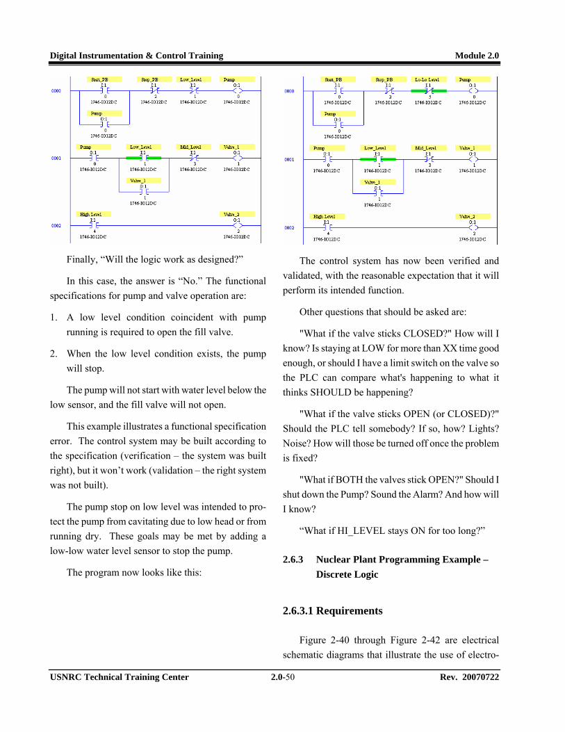
Digital Instrumentation & Control Training Module 2.0
USNRC Technical Training Center 2.0-50 Rev. 20070722
Finally, “Will the logic work as designed?”
In this case, the answer is “No.” The functional specifications for pump and valve operation are:
1. A low level condition coincident with pump running is required to open the fill valve.
2. When the low level condition exists, the pump will stop.
The pump will not start with water level below the low sensor, and the fill valve will not open.
This example illustrates a functional specification error. The control system may be built according to the specification (verification – the system was built right), but it won’t work (validation – the right system was not built).
The pump stop on low level was intended to pro-tect the pump from cavitating due to low head or from running dry. These goals may be met by adding a low-low water level sensor to stop the pump.
The program now looks like this:
The control system has now been verified and validated, with the reasonable expectation that it will perform its intended function.
Other questions that should be asked are:
"What if the valve sticks CLOSED?" How will I know? Is staying at LOW for more than XX time good enough, or should I have a limit switch on the valve so the PLC can compare what's happening to what it thinks SHOULD be happening?
"What if the valve sticks OPEN (or CLOSED)?" Should the PLC tell somebody? If so, how? Lights? Noise? How will those be turned off once the problem is fixed?
"What if BOTH the valves stick OPEN?" Should I shut down the Pump? Sound the Alarm? And how will I know?
“What if HI_LEVEL stays ON for too long?”
2.6.3 Nuclear Plant Programming Example – Discrete Logic
2.6.3.1 Requirements
Figure 2-40 through Figure 2-42 are electrical schematic diagrams that illustrate the use of electro-

Digital Instrumentation & Control Training Module 2.0
USNRC Technical Training Center 2.0-51 Rev. 20070722
magnetic relays to implement Steam Dump control in a nuclear power plant. The diagrams do not show analog devices that are part of the control system. The drawings are accurate representations of the design; in fact, they ARE the design. The drawings also show some of the drawbacks to building even moderately complex control systems with relay devices:
• Many of the relays are “auxiliary” relays. That is, they are relays whose function is to provide more contacts than a single relay can provide.
• The addition of auxiliary relays increases the device count, which reduces reliability.
• It is difficult to trace control functions through the schematic.
2.6.3.2 Ladder Logic Representation
The Triconex TS1131 configuration tool is used for this example. Figure 2-43 illustrates the literal transformation of a portion of the schematic represen-tations in Figure 2-40 through Figure 2-42 to ladder logic representation for a single atmospheric steam dump valve, PCV-19. Figure 2-43 clearly shows the issues associated with relay logic. Specifically, the number of auxiliary relays being used for contact multiplication functions. Note that the ladder logic representation illustrates the relationship of the auxiliary relays more clearly than the schematic.
2.6.3.3 Function Block Diagram Representa-tion
Figure 2-44 illustrates translation of the PCV-19 electrical schematic into the IEC 61131-3 Function Block Diagram notation. Physical relays have been replaced with symbolic names, simplifying the program.
2.6.4 Another Nuclear Plant Programming Example
Figure 2-45 illustrates the functional representa-tion of the Westinghouse high pressurizer pressure reactor trip function as it could be implemented in the SSPS described previously in this lesson. The bistable outputs from the process protection system are energized below the trip setpoint and deenergized above the setpoint. In Figure 2-46, the functional representation has been translated into ladder logic using the Triconex TS1131 programming tool. In this example, the code is annotated to explain its operation. Figure 2-47 illustrates the IEC61131-3 function block representation. In both ladder logic and function block representations, the code is entered by copying and pasting elements using the programming tool editor. When copying and pasting, subtle errors can be introduced if variable name assignments are not edited very carefully. Figure 2-48 illustrates the use of a custom function block that implements the 2oo4 logic function block developed in Figure 2-36. Use of the custom function block reduces the editing needed to develop a function, and is much easier to understand. However, custom function blocks that have not been subjected to the PLC suppliers must be verified and validated against approved specifications if they are to be used in safety-related applications.
Finally, Figure 2-49 illustrates use of structured text to illustrate how custom functions can be coded directly when the library supplied by the programming tool manufacturer does not contain a needed block. Typically, the structured text would be used to build a custom function block, rather than to implement an entire function as shown in Figure 2-48.
2.6.5 Graphical User Interface for HMI
Graphical displays are used to monitor and some-times control the plant process. The display represents

Digital Instrumentation & Control Training Module 2.0
USNRC Technical Training Center 2.0-52 Rev. 20070722
motors, pipes, valves, tanks, and other process equip-ment with graphical objects, as shown for the pump problem discussed in Section 2.6.2. System status data is overlaid on those objects. Typically, the graphical interface development software offered by a manufac-turer can be linked to the emulator tools offered by the same manufacturer. As an example, Figure 2-50 illustrates the real-time emulation of the final pump ladder logic diagram shown on page 2.0-49. Figure 2-51 reflects an active Graphical User Interface (GUI) to the real-time emulation model. The emulation model is usually not distinguishable from operation with a “Live” PLC.
The PLC system network requires high data trans-mission rates to support graphical displays. If the system network is not fast enough, the terminal may not display the most current data. In addition, the communications between the PLC processor and the graphic display terminal may delay the processor's reaction to a system fault or required process change.
2.6.6 Programming Tools
Personal computer-based software to aid in the design, implementation, debugging, emulation, and documentation of the application program is offered by virtually all PLC manufacturers.
A few PLC manufacturers offer simulators, but most simulators must be purchased through third-party vendors. Simulators may be either special packaged units independent of the PLC system or I/O modules that mount directly into the PLC racks. The packaged units can range from simple switches and indicators to complex CPU based simulators. I/O module simulators replace a specific manufacturer's I/O module and simulate the module's operation to the PLC processor. Simulators are used to verify correct operation of the user program, the PLC system (including the proces-
sor, communications, and the I/O modules), and the field devices.
Emulators are software-based tools used to verify proper operation of the program. Emulators allow the programming terminal to operate in the on-line mode without being physically connected to a PLC system. The emulator reads and solves the logic program and (transmits) the necessary display information to the programming terminal. The PLC processor or its I/O modules are never communicated with nor controlled.
Both simulators and emulators are useful tools in troubleshooting and debugging PLC software and hardware. In addition, simulators and emulators can be used to play "what if" games and validate correct system responses to presented threats. When develop-ing nuclear safety-related applications, it is important to know whether the specific tools being used have been included in the manufacturer’s SER for use in performing development as well as Verification and Validation (V&V). Custom function blocks that were not included in the supplier’s SER must be subjected to an equivalent level of verification and validation if they are to be used in safety-related applications.

Bus Name Description PC/AT Bus used in early IBM-compatible computers to connect peripheral devices such as
disk drive and sound cards to the motherboard of the computer. PCI Another bus used in personal computers, but not limited to IBM-compatibles. Much
faster than PC/AT. Typical data transfer rate of 100 Mbytes/second (32 bit) and 200 Mbytes/second (64 bit).
PCMCIA A bus designed to connect peripherals to laptop and notebook sized personal com-puters. Has a very small physical "footprint," but is considerably slower than other popular PC buses.
VME A high-performance bus (co-designed by Motorola, and based on Motorola's earlier Versa-Bus standard) for constructing versatile industrial and military computers, where multiple memory, peripheral, and even microprocessor cards could be plugged in to a passive "rack" or "card cage" to facilitate custom system designs. Typical data transfer rate of 50 Mbytes/second (64 bits wide).
VXI An expansion of the VME bus, VXI (VME eXtension for Instrumentation) includes the standard VME bus along with connectors for analog signals between cards in the rack.
S-100 Sometimes called the Altair bus, this bus standard was the product of a conference in 1976, intended to serve as an interface to the Intel 8080 microprocessor chip. Similar in philosophy to the VME, where multiple function cards could be plugged in to a passive "rack," facilitating the construction of custom systems.
MC6800 The Motorola equivalent of the Intel-centric S-100 bus, designed to interface peripheral devices to the popular Motorola 6800 microprocessor chip.
STD Stands for Simple-To-Design, and is yet another passive "rack" similar to the PC/AT bus, and lends itself well toward designs based on IBM-compatible hardware. Designed by Pro-Log, it is 8 bits wide (parallel), accommodating relatively small (4.5 inch by 6.5 inch) circuit cards.
Multibus I and II Another bus intended for the flexible design of custom computer systems, designed by Intel. 16 bits wide (parallel).
CompactPCI An industrial adaptation of the personal computer PCI standard, designed as a higher-performance alternative to the older VME bus. At a bus clock speed of 66 MHz, data transfer rates are 200 Mbytes/ second (32 bit) or 400 Mbytes/sec (64 bit).
Microchannel channel Yet another bus, this one designed by IBM for their ill-fated PS/2 series of computers, intended for the interfacing of PC motherboards to peripheral devices.
IDE A bus used primarily for connecting personal computer hard disk drives with the appropriate peripheral cards. Widely used in today's personal computers for hard drive and CD-ROM drive interfacing.
SCSI An alternative (technically superior to IDE) bus used for personal computer disk drives. SCSI stands for Small Computer System Interface. Used in some IBM-compatible PC's, as well as Macintosh (Apple), and many mini and mainframe business computers. Used to interface hard drives, CD-ROM drives, floppy disk drives, printers, scanners, modems, and a host of other peripheral devices. Speeds up to 1.5 Mbytes per second for the original standard.
GPIB (IEEE 488) General Purpose Interface Bus, also known as HPIB or IEEE 488, which was intended for the interfacing of electronic test equipment such as oscilloscopes and multimeters to personal computers. 8 bit wide address/data "path" with 8 additional lines for communications control.
Centronics parallel Widely used on personal computers for interfacing printer and plotter devices. Sometimes used to interface with other peripheral devices, such as external ZIP (100 Mbyte floppy) disk drives and tape drives.

Bus Name Description USB Universal Serial Bus, which is intended to interconnect many external peripheral
devices (such as keyboards, modems, mice, etc.) to personal computers. Long used on Macintosh PC's, it is now being installed as new equipment on IBM-compatible machines.
FireWire (IEEE 1394)
A high-speed serial network capable of operating at 100, 200, or 400 Mbps with versatile features such as "hot swapping" (adding or removing devices with the power on) and flexible topology. Designed for high-performance personal computer interfacing.
Bluetooth A radio-based communications network designed for office linking of computer devices. Provisions for data security designed into this network standard.
Table 2-1 Short-Distance Busses
Bus Name Description
20 mA current loop Not to be confused with the common instrumentation 4-20 mA analog standard, this is a digital communications network based on interrupting a 20 mA (or sometimes 60 mA) current loop to represent binary data. Although the low impedance gives good noise immunity, it is susceptible to wiring faults (such as breaks) which would fail the entire network.
RS-232C The most common serial network used in computer systems, often used to link peripheral devices such as printers and mice to a personal computer. Limited in speed and distance (typically 45 feet and 20 kbps, although higher speeds can be run with shorter distances). I've been able to run RS-232 reliably at speeds in excess of 100 kbps, but this was using a cable only 6 feet long! RS-232C is often referred to simply as RS-232 (no "C").
RS-422A/RS-485 Two serial networks designed to overcome some of the distance and versatility limitations of RS-232C. Used widely in industry to link serial devices together in electrically "noisy" plant environments. Much greater distance and speed limita-tions than RS-232C, typically over half a mile and at speeds approaching 10 Mbps.
Ethernet (IEEE 802.3)
A high-speed network which links computers and some types of peripheral devices together. "Normal" Ethernet runs at a speed of 10 million bits/second, and "Fast" Ethernet runs at 100 million bits/second. The slower (10 Mbps) Ethernet has been implemented in a variety of means on copper wire (thick coax = "10BASE5", thin coax = "10BASE2", twisted-pair = "10BASE-T"), radio, and on optical fiber ("10BASE-F"). The Fast Ethernet has also been implemented on a few different means (twisted-pair, 2 pair = 100BASE-TX; twisted-pair, 4 pair = 100BASE-T4; optical fiber = 100BASE-FX).
Token ring Another high-speed network linking computer devices together, using a philoso-phy of communication that is much different from Ethernet, allowing for more precise response times from individual network devices, and greater immunity to network wiring damage.

Bus Name Description
FDDI A very high-speed network exclusively implemented on fiber-optic cabling.
Modbus/Modbus Plus Originally implemented by the Modicon corporation, a large maker of Program-mable Logic Controllers (PLCs) for linking remote I/O (Input/Output) racks with a PLC processor. Still quite popular.
Profibus Originally implemented by the Siemens corporation, another large maker of PLC equipment.
Foundation Fieldbus A high-performance bus expressly designed to allow multiple process instruments (transmitters, controllers, valve positioners) to communicate with host computers and with each other. May ultimately displace the 4-20 mA analog signal as the standard means of interconnecting process control instrumentation in the future.
Table 2-2 Extended-Distance Networks


Required Integrity Low Med High V&V Class V&V Intensity Low
3 3 2 3 Least Rigorous
Med
2 2 2 2 Intermediate
Complexity
High
2 2 1 1 Most Rigorous
Figure 2-1 EPRI TR-103291 Graded Quality Concept
Figure 2-2 Analog Controller – Discrete Component Technology

Figure 2-3 Typical Industrial Control Relay
Figure 2-4 Typical Rotary Power Relay (Seismically Qualified)

Figure 2-5 Typical Pneumatic Time Delay Relay

Figure 2-6 Westinghouse SSPS PWR Protection Scheme

Figure 2-7 Westinghouse SSPS Functions

Figure 2-8 Westinghouse SSPS Input Relays
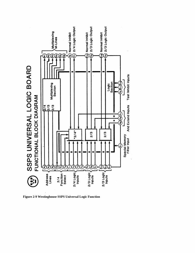
Figure 2-9 Westinghouse SSPS Universal Logic Function

Figure 2-10 Westinghouse SSPS Universal Logic Circuit Card

Figure 2-11 Westinghouse SSPS UV Driver Function
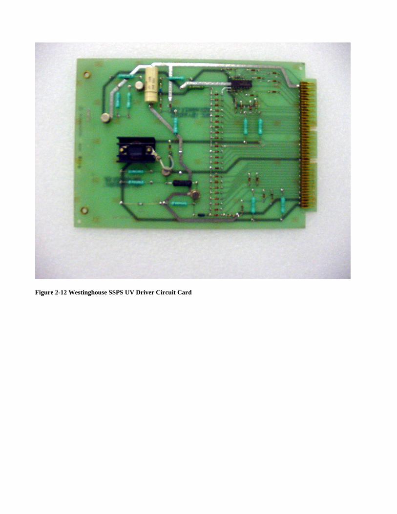
Figure 2-12 Westinghouse SSPS UV Driver Circuit Card

Figure 2-13 Westinghouse SSPS SAF Driver Function;
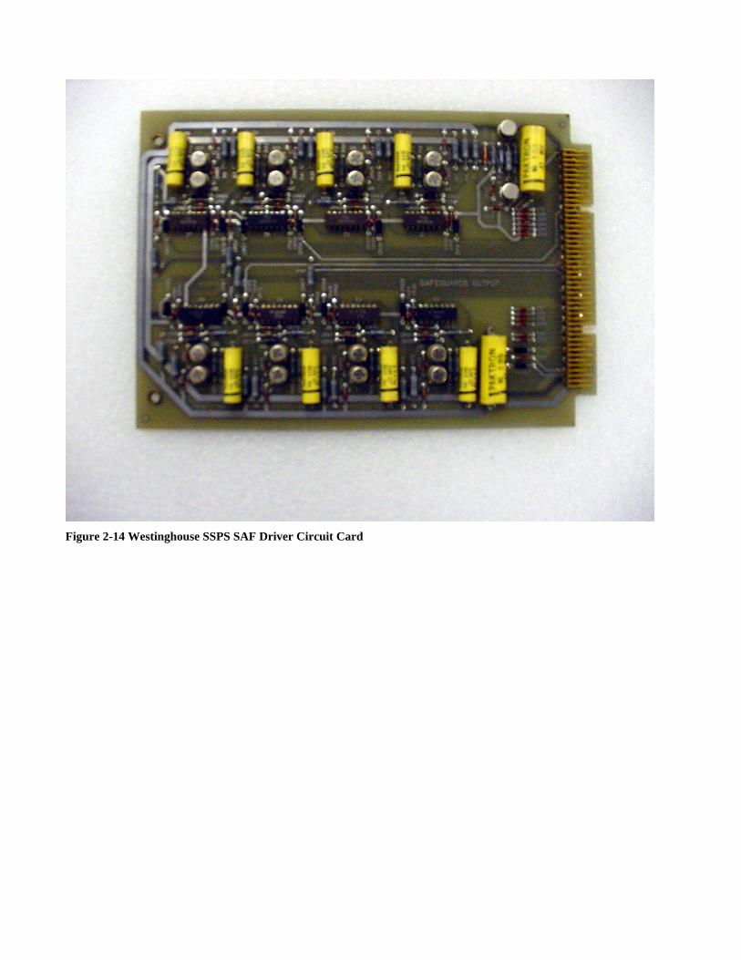
Figure 2-14 Westinghouse SSPS SAF Driver Circuit Card
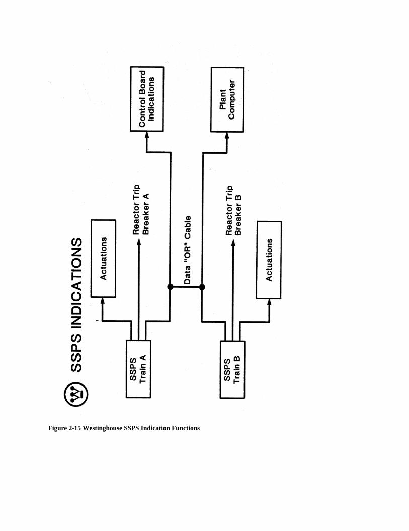
Figure 2-15 Westinghouse SSPS Indication Functions

ProgrammableController
Processor Machine
Control
Measure
FieldInputs
FieldOutputs
Figure 2-16 Industrial Computer (PLC) Concept

Figure 2-17 Typical Industrial Control Ladder Diagram (Portion)
Figure 2-18 Simple Ladder Logic Program

Figure 2-19 Typical Industrial Programmable Controller
Figure 2-20 Typical Analog Process Loop

Figure 2-21 DCS Concept
Figure 2-22 Shared Function Controller

Figure 2-23 Individual Loop Controller
Figure 2-24 Single Control Module
Input Circuits
CPU
Memory
Output Circuits
InputRelays
CountersOutputRelays
InternalRelays
TimersData
Storage
PowerSupply
Figure 2-25 Inside the PLC

Figure 2-26 PLC Input Structure

Figure 2-27 PLC Output Structure

Scan Inputs
Execute Program
Update Outputs
Housekeeping &Diagnostics
Start
Repeat Cycle Time
Figure 2-28 PLC Run-Mode Operation
O N
In p u tP ro g ra m
E xe c O u tp u t
S ca n 1
In p u tP ro g ra m
E xe c O u tp u t
S ca n 2
Inp u tP ro g ra m
E xe c O u tp u t
S can 3
O F F
1 2 3
O u tp u t In p u t
In p u t 1 n o t se e n u n til S ca n 2In p u t 2 n o t se e n u n til S ca n 3W h a t a b o u t Inp u t 3 ?
S ca n 4
Figure 2-29 Affects of Scan Cycle on Response Time

ON
InputProgram
Exec Output
Scan 1
InputProgram
Exec Output
Scan 2
InputProgram
Exec Output
Scan 3
OFF
Output Input
Scan 4InputDelay
t0 t1 t2
t0: Scan 1 startst1: Input turns ont2: Output turns on at end of Scan 2 output phaseMax Time Response = 2 * Scan - (t1 - t0)
Input Output
Figure 2-30 Maximum Response Time
Figure 2-31 Scan Time Allocation

Figure 2-32 Remote I/O Using Peer-to-Peer Communications
Figure 2-33 Programming Examples

Figure 2-34 Object-Oriented Programming
Figure 2-35 Function Blocks

Figure 2-36 Typical Custom Function Block (2oo4) Coincidence Logic
Figure 2-37 Multifunction Control Algorithms
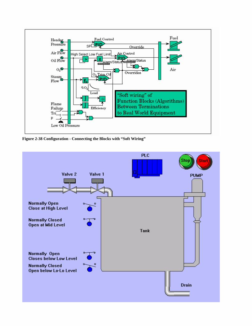
Figure 2-38 Configuration - Connecting the Blocks with “Soft Wiring”

Figure 2-39 PLC Programming Problem
Figure 2-40 Steam Dump Control Schematic Diagram
Figure 2-41 Auxiliary Relays Schematic Diagram

Figure 2-42 Steam Dump Valve Control Schematic Diagram
Figure 2-43 Relay Logic Transformation to Ladder Logic Program

Figure 2-44 Relay Logic Transformation to Function Block Diagram Program
Figure 2-45 Pressurizer Pressure Protection Functional Diagram

Figure 2-46 Pressurizer Pressure Protection Ladder Logic Program
Figure 2-47 Pressurizer Pressure Protection Function Block Diagram Program
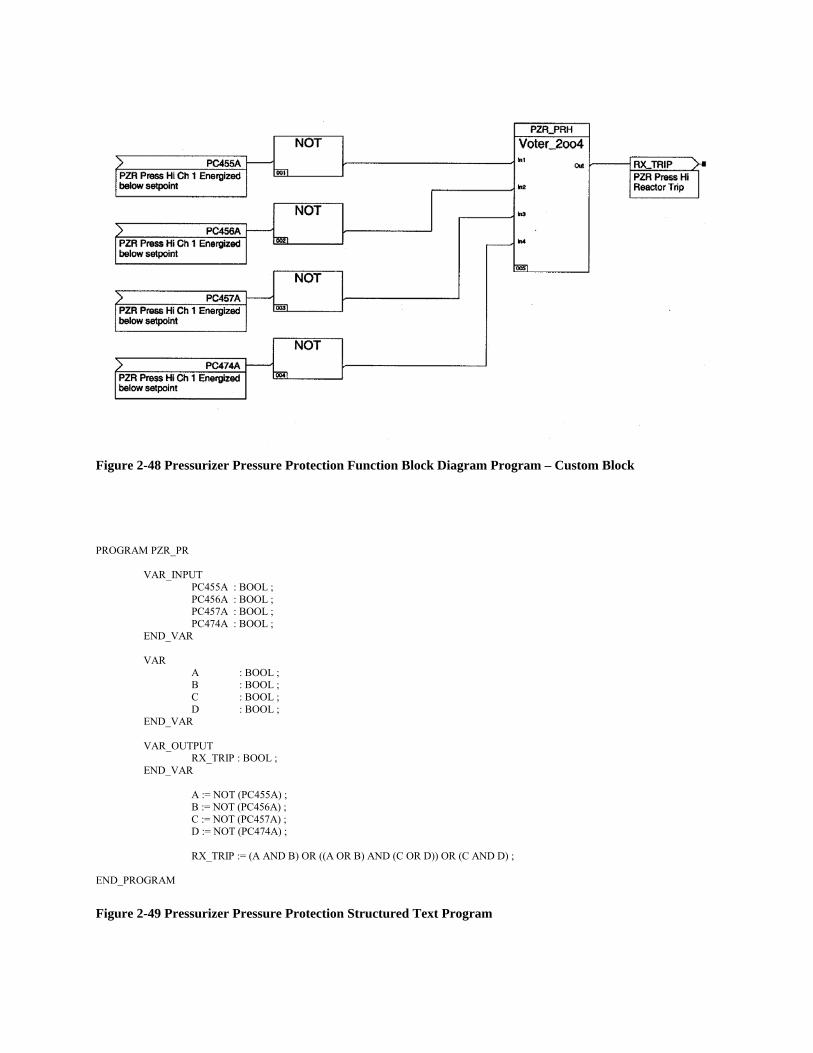
Figure 2-48 Pressurizer Pressure Protection Function Block Diagram Program – Custom Block
PROGRAM PZR_PR VAR_INPUT PC455A : BOOL ; PC456A : BOOL ; PC457A : BOOL ; PC474A : BOOL ; END_VAR VAR A : BOOL ; B : BOOL ; C : BOOL ; D : BOOL ; END_VAR VAR_OUTPUT RX_TRIP : BOOL ; END_VAR A := NOT (PC455A) ; B := NOT (PC456A) ; C := NOT (PC457A) ; D := NOT (PC474A) ; RX_TRIP := (A AND B) OR ((A OR B) AND (C OR D)) OR (C AND D) ; END_PROGRAM Figure 2-49 Pressurizer Pressure Protection Structured Text Program

Figure 2-50 Emulation Tool Connected to HMI Display

Figure 2-51 Object-Oriented HMI Display

Figure 2-52 Triconex Triple Mode Redundant PLC (with SER)

Figure 2-53 Siemens Teleperm XS PLC (with SER)

Bistable Processor Coincidence Processor Independent Test Processor
Figure 2-54 Westinghouse Common Q (AC160) PLC Rack Figure 2-54 Westinghouse Common Q (AC160) PLC Rack
Figure 2-55 Westinghouse Common Q Qualified Flat Panel Display


