Digital Image Processing & Pattern Analysis (CSCE 563) Intensity Transformations Prof. Amr Goneid...
44
Digital Image Processing & Pattern Analysis (CSCE 563) Intensity Transformations Prof. Amr Goneid Department of Computer Science & Engineering The American University in Cairo
-
Upload
lizbeth-cook -
Category
Documents
-
view
232 -
download
1
Transcript of Digital Image Processing & Pattern Analysis (CSCE 563) Intensity Transformations Prof. Amr Goneid...

Digital Image Processing&
Pattern Analysis(CSCE 563)
Intensity Transformations
Digital Image Processing&
Pattern Analysis(CSCE 563)
Intensity Transformations
Prof. Amr GoneidDepartment of Computer Science & Engineering
The American University in Cairo

Prof. Amr Goneid, AUC 2
Intensity TransformationsIntensity Transformations
Pixel Intensity Processing
Histogram Processing
Combining Images

Prof. Amr Goneid, AUC 3
Pixel Intensity Processing
Point Processing
Gray Scale to Binary
Negative
Power Law Transformation
Contrast Stretching
Compression of Dynamic Range
Gray Level Slicing

Prof. Amr Goneid, AUC 4
Point Processing
Local Processing:g(x,y) = T[f(x,y)]
T = Operator on Locality (neighborhood) of (x,y)
e.g. 3 x 3 T [ ] (8-neighborhood)
Point Processing:For 1 x 1 we have Point Processing
S = T[r] = T[ ]S = New Intensity, r = Old Intensity
p

Prof. Amr Goneid, AUC 5
Gray scale to Binary
s = T(r,a) = 0 for r < a, 1 otherwise

Prof. Amr Goneid, AUC 6
Negative (Image Complement)
s =T(r) = 1-r
The MATLAB function:
g = imcomplement(f)
10 r
1
s

Power Law Transformation
Has the form:
The MATLAB function
g = imadjust (f, [low-in high-in], [low-out high-out], gamma)
Prof. Amr Goneid, AUC 7
crs
Power Law TransformationExample:
g = imadjust (f, [0 1], [1 0]);
equivalent to: g = imcomplement (f);
g = imadjust (f, [0.3 0.7], [0.2 1.0]);
Prof. Amr Goneid, AUC 8

Prof. Amr Goneid, AUC 9
Contrast Stretching
Low contrast images do not make full use of the dynamic range of grey levels. In this case the intensities are confined to a narrow range rmin < r < rmax.
We can use a point transformation s = T(r) to stretch the range to smin < s < smax

Prof. Amr Goneid, AUC 10
Contrast Stretching
r = old intensity, s = new intensity
Slope = s/ r > 1 produces
contrast stretching. = [(smax– smin)/(rmax– rmin)]
Hence, s =T(r)
= (r – rmin) + smin
r
s
r
s

Prof. Amr Goneid, AUC 11
Contrast Stretching Example
rmin = 0.0 , rmax = 0.3 smin = 0.0 , smax = 1.0

Contrast Stretching Function
Prof. Amr Goneid, AUC 12
mrforandmrfors
rmrTs
E
E
10lim that Notice
)/(1
1)(
•The function compresses the input
levels lower than m into a narrow
range of dark levels in the output image.
• Similarly, it compresses intensities
above m into a narrow band of light
levels in the output.
•The result is an image of higher contrast.
Contrast Stretching Function
Summer 2009 Prof. Amr Goneid, AUC 13
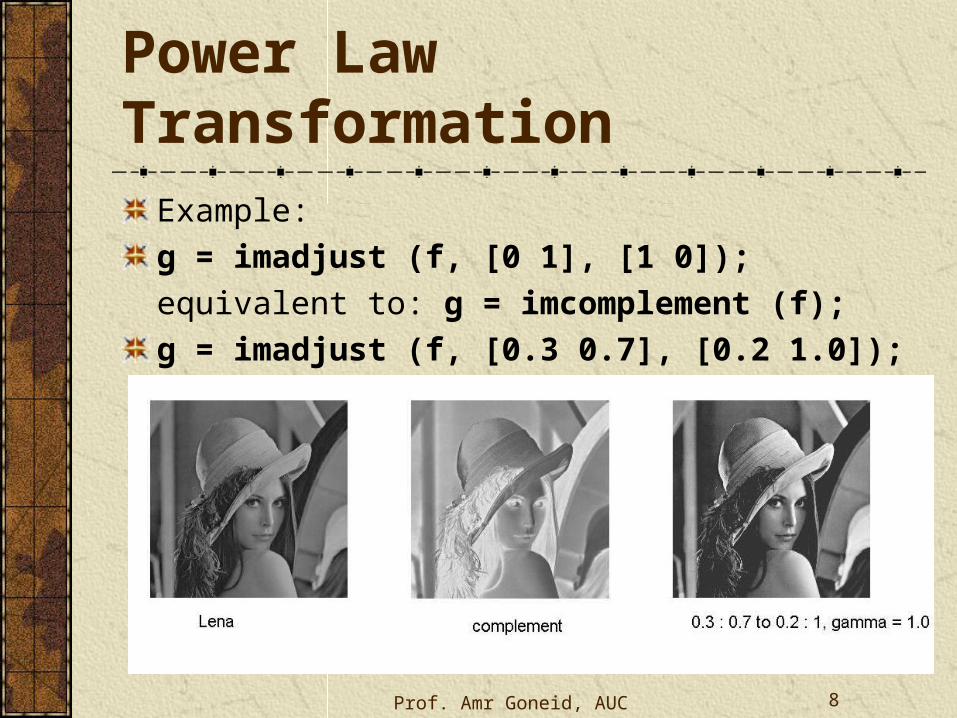
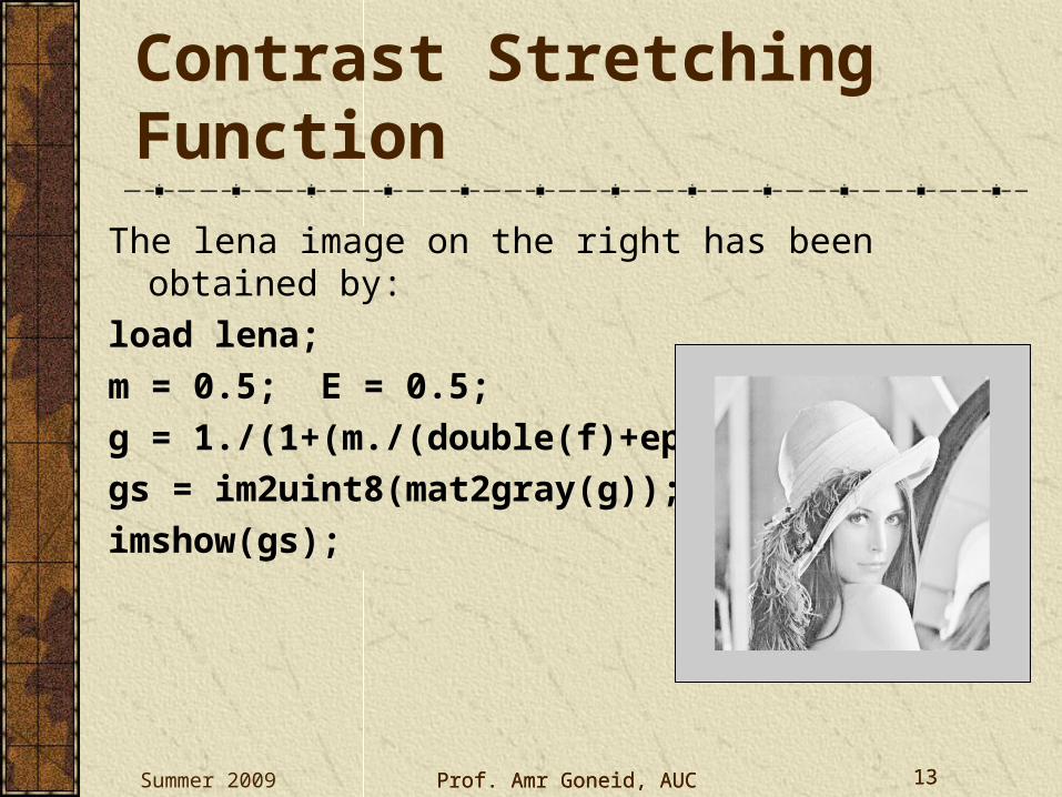
The lena image on the right has been obtained by:
load lena;
m = 0.5; E = 0.5;
g = 1./(1+(m./(double(f)+eps)).^E);
gs = im2uint8(mat2gray(g));
imshow(gs);
13Prof. Amr Goneid, AUC

Contrast Stretching Function
Summer 2009 Prof. Amr Goneid, AUC 14
In the limiting case it produces a binary image.
14Prof. Amr Goneid, AUC

Summer 2009 Prof. Amr Goneid, AUC 15
Compression of Dynamic Range
Map r = {0,D} to s = {0,L-1}
where D >> L-1
s = T(r) = c log(1 + r )
c = (L-1)/log(1+D)
e.g. compression from
256 gray levels
to 16 gray levels.
15Prof. Amr Goneid, AUC

Prof. Amr Goneid, AUC 16
Gray Level Slicing
Examples:S = T(r)
= {1 for A<r<B ;
c otherwise}
S = T(r)
= {1 for r>A; r otherwise}
s
rs
r
1
0
0
1
1
1A
A B
c

Prof. Amr Goneid, AUC 17
Gray Level Slicing Example
S = T(r) = {1 for r>0.6; r otherwise}

Prof. Amr Goneid, AUC 18
Histogram Processing
A bad contrast image (F) can be enhanced to an image G by transforming every pixel intensity fij to another intensity gij using a method called Histogram Equalization

Prof. Amr Goneid, AUC 19
Histogram Processing
PDF and CDF
Histogram Equalization (Theory)
Histogram Equalization (Practice)
Histogram Specification
Prof. Amr Goneid, AUC 20
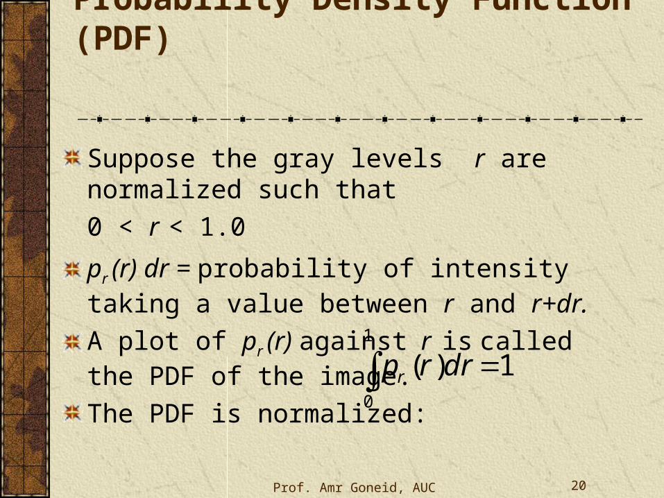
Probability Density Function (PDF)
Suppose the gray levels r are normalized such that
0 < r < 1.0
pr (r) dr = probability of intensity taking a value between r and r+dr.
A plot of pr (r) against r is called the PDF of the image.
The PDF is normalized: 1
0
1)( drrpr

Prof. Amr Goneid, AUC 21
Cumulative Distribution Function (CDF)
The CDF = the probability of having values less than r
For a uniform PDF, ps (s) = 1 and CDF = s
(i.e. CDF is Linear)
r
rr drrprpCDF0
)()(
Uniform
cdf

Prof. Amr Goneid, AUC 22
Histogram Equalization (Theory)
TooDark
BadContrast
TooBright
P(r)
r
UniformHigh Contrast
P(s)
s
Mapping r into s such that ps (s) is uniform
Prof. Amr Goneid, AUC 23
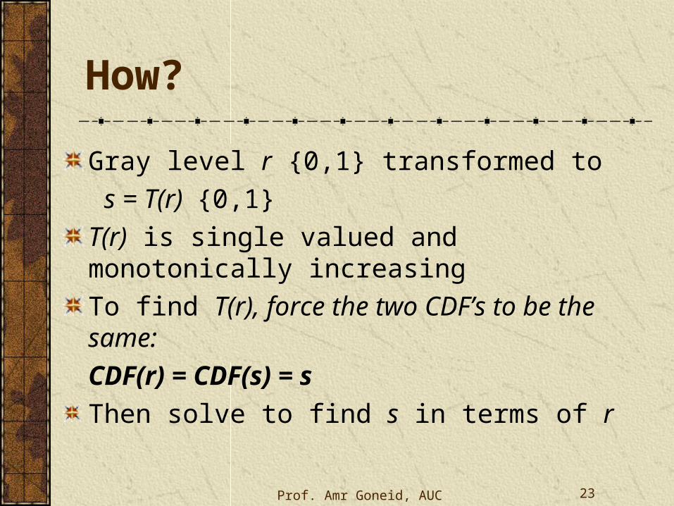
How?
Gray level r {0,1} transformed to
s = T(r) {0,1}
T(r) is single valued and monotonically increasing
To find T(r), force the two CDF’s to be the same:
CDF(r) = CDF(s) = s
Then solve to find s in terms of r

Prof. Amr Goneid, AUC 24
Example
2
0 1
10 also that Notice
)1(1)()(
)1(2)(givesion Normalizat
10)1()(Consider
2
0
s
rdrrprCDFs
rrp
rrrp
r
r
r
r
Prof. Amr Goneid, AUC 25
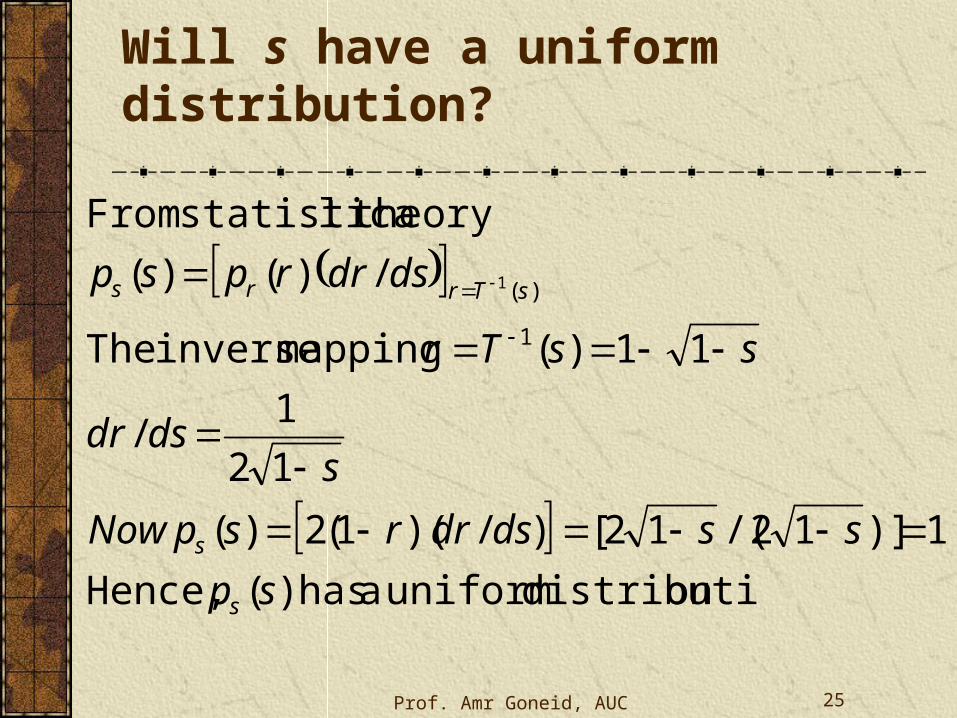
Will s have a uniform distribution?
on distributi uniform a has)( Hence,
1)]12/(12[)/)(1(2)(
12
1/
11)( mapping inverse The
/)()(
theorylstatistica From
1
)(1
sp
ssdsdrrspNow
sdsdr
ssTr
dsdrrpsp
s
s
sTrrs

Prof. Amr Goneid, AUC 26
Histogram Equalization (Practice)
In practice, gray levels are discrete (k = 0 .. L-1)
A histogram is an array whose element nk = no. of pixels with gray level k (k = 0 is black, k = L-1 is white).
A histogram is a plot of nk vs rk e.g. for L = 256
In MATLAB
n = imhist(I,256)
Prof. Amr Goneid, AUC 27
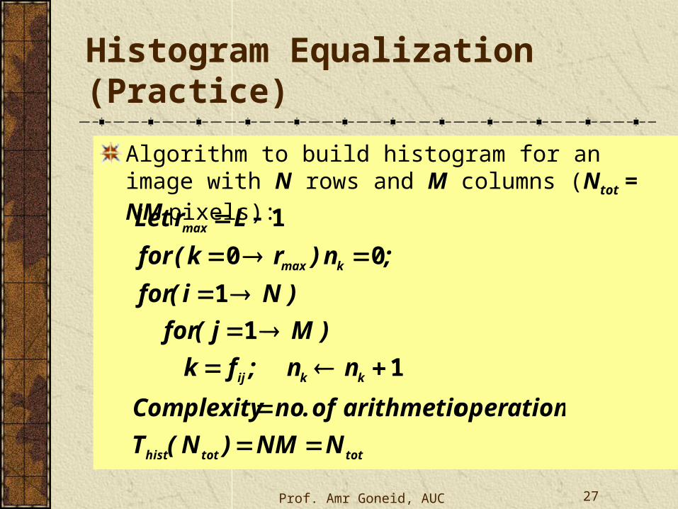
Histogram Equalization (Practice)
Algorithm to build histogram for an image with N rows and M columns (Ntot = NM pixels):
tottothist
kkij
kmax
max
NNM)N(T
operationsarithmeticof.noComplexity
nn;fk
)Mj(for
)Ni(for
;n)rk(for
LrLet
1
1
1
00
1
Prof. Amr Goneid, AUC 28
Histogram EqualizationHistogram EqualizationAlgorithm (1)Algorithm (1)
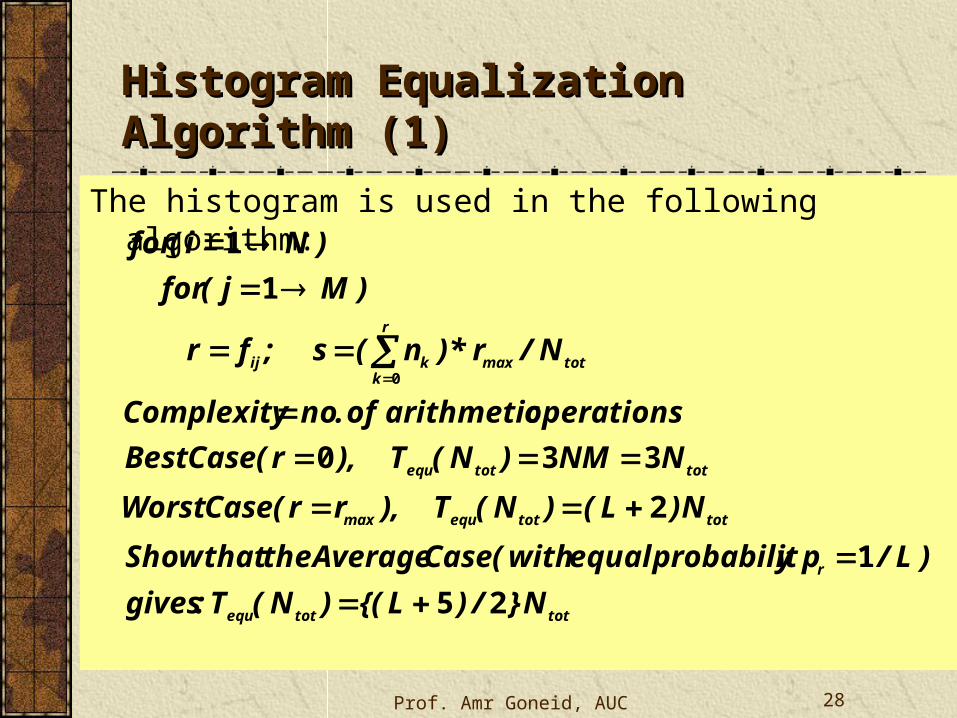
The histogram is used in the following algorithm:
tottotequ
r
tottotequmax
tottotequ
totmax
r
kkij
N}/)L{()N(T:gives
)L/pyprobabilitequalwith(CaseAveragethethatShow
N)L()N(T),rr(CaseWorst
NNM)N(T),r(CaseBest
operationsarithmeticof.noComplexity
N/r*)n(s;fr
)Mj(for
)Ni(for
25
1
2
330
1
1
0

Prof. Amr Goneid, AUC 29
Histogram EqualizationHistogram EqualizationAlgorithm (2)Algorithm (2)
A better algorithm first builds a Cumulative array:
)L(N)N(T
N/r*Cg;fr
)Mj(for
)Ni(for
:ituseweThen
Lroperationsarithmeticof.no
sumC;nsumsum
)rk(for
;sumC;nsum
tottotequ
totmaxrijij
max
kk
max
12
1
1
1
100

Prof. Amr Goneid, AUC 30
Histogram EqualizationHistogram EqualizationSummary of Total ComplexitySummary of Total Complexity
Algorithm (1):
Algorithm (2):
tottot
tottotmax
tottot
N}/)L{()N(TCaseAverage
N)L()N(T),rr(CaseWorst
N)N(T),r(CaseBest
27
3
40
)L(N)N(TCasesAll tottot 13

Prof. Amr Goneid, AUC 31
Histogram EqualizationHistogram EqualizationNumerical ExampleNumerical Example
L = 256 gray levels
Algorithm (1):
Algorithm (2):
tottot
tottotmax
tottot
N.)N(TCaseAverage
N)N(T),rr(CaseWorst
N)N(T),r(CaseBest
5131
259
40
2553 tottot N)N(TCasesAll

Summer 2009 Prof. Amr Goneid, AUC 32
Histogram Equalization (Practice)
If N = total no. of pixels = numel (I), then the PDF of input image is Pr(rk) = n(k)/N
L)histeq(f, g
MATLAB, In
into level transform will nqualizatio Histogram
)(
)()(1
kk
kk
j
k
jrk
rCDFs
sr
rprCDF
32Prof. Amr Goneid, AUC

Prof. Amr Goneid, AUC 33
Practical ExamplesFrom: http://www.ph.tn.tudelft.nl/Courses/FIP/noframes/fip.html
Original Contrast
Stretched
Histogram
Equalized

Prof. Amr Goneid, AUC 34
Negative Ramp

Prof. Amr Goneid, AUC 35
Liver Tissue Image

Summer 2009 Prof. Amr Goneid, AUC 36
Girl Image
36Prof. Amr Goneid, AUC

Prof. Amr Goneid, AUC 37
Histogram Specification
How to Transform an image (A) with Pr(r) to an image (B) with specified Pz(z).
For the input image (A), the uniform variable s = T(r) = CDF(r) For the output image (B), s = H(z) = CDF(z) Hence z = H-1(s) = H-1(T(r))In MATLAB: g = histeq (f , HistB)
Summer 2009 Prof. Amr Goneid, AUC 38
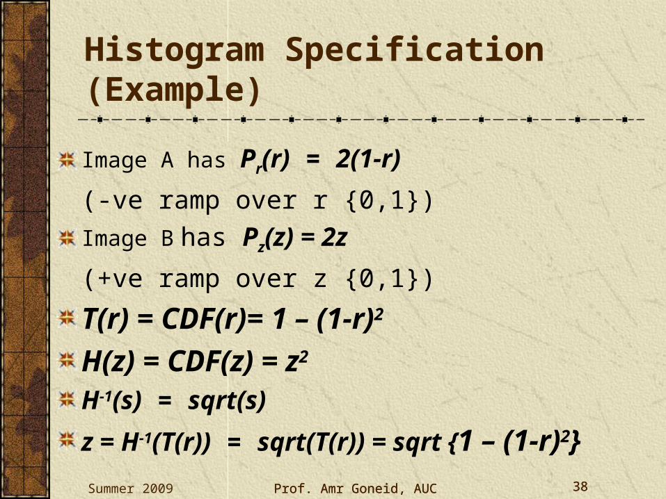
Histogram Specification (Example)
Image A has Pr(r) = 2(1-r)
(-ve ramp over r {0,1})
Image B has Pz(z) = 2z
(+ve ramp over z {0,1})
T(r) = CDF(r)= 1 – (1-r)2
H(z) = CDF(z) = z2 H-1(s) = sqrt(s)
z = H-1(T(r)) = sqrt(T(r)) = sqrt {1 – (1-r)2}38Prof. Amr Goneid, AUC

Prof. Amr Goneid, AUC 39
A Practical Example(-)ve To (+)ve Ramp

Prof. Amr Goneid, AUC 40
Combining Images
Arithmetic Operations
Logical Operations

Prof. Amr Goneid, AUC 41
Combining Images
By Arithmetic Operations:e.g. Addition & Subtraction:C = min (A + B , 1);C = max (A – B , 0);
By Logical operations(Binary Images):C = A & B Logical ANDC = A | B Logical ORC = A xor B Logical Exclusive ORC = ~ A Logical NOT

Prof. Amr Goneid, AUC 42
Example: Arithmetic
I=Image; RN = Random Noise; B=boundary
I + RN + B RN - I

Prof. Amr Goneid, AUC 43
Example: Logical
Mask AND Image1 = Image2
Prof. Amr Goneid, AUC 44
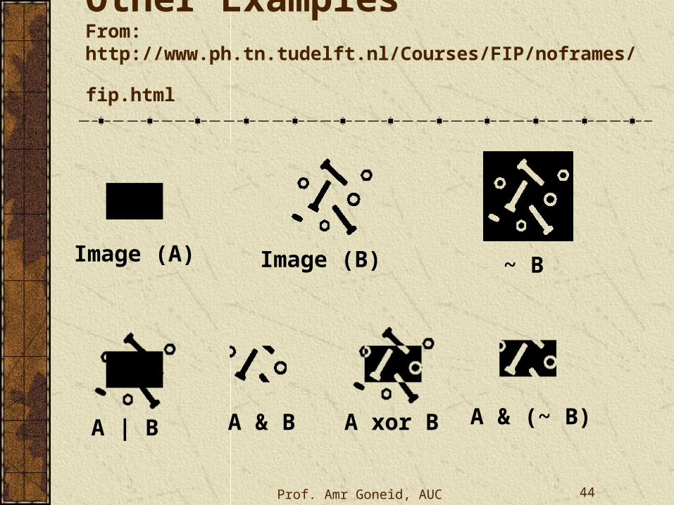
Other ExamplesFrom: http://www.ph.tn.tudelft.nl/Courses/FIP/noframes/fip.html
Image (A) Image (B) ~ B
A | B A & B A xor B A & (~ B)