Digital Climatic Atlas of · PDF fileDigital Climatic Atlas of Texas Final Project Report...
108
Digital Climatic Atlas of Texas Final Project Report prepared by Balaji Narasimhan Raghavan Srinivasan Steven Quiring John W. Nielsen-Gammon Texas A&M University College Station, Texas – 77843 Submitted to The Texas Water Development Board for completion of TWDB contract # 2005-483-559 1
Transcript of Digital Climatic Atlas of · PDF fileDigital Climatic Atlas of Texas Final Project Report...

Digital Climatic Atlas of Texas
Final Project Report
prepared by
Balaji Narasimhan Raghavan Srinivasan
Steven Quiring John W. Nielsen-Gammon
Texas A&M University
College Station, Texas – 77843
Submitted to
The Texas Water Development Board
for completion of
TWDB contract # 2005-483-559
1

Digital Climatic Atlas of Texas
Executive Summary
A digital climatic atlas of Texas has been created that defines the climate in terms
of major climatic parameters, precipitation, maximum and minimum temperatures and
lake evaporation. Datasets from wide-ranging sources of varying quality and resolutions
were processed and assembled to create this comprehensive dataset of monthly and
annual decadal means both in gridded (4 km) and point format for 11 decades from 1890
to 2000. The datasets used to develop these gridded and point decadal means went
through a variety of QA/QC procedures, data homogenization and infilling techniques to
create the best possible serially complete data for estimating long-term decadal means.
The accuracy of gridded datasets of precipitation and temperature obtained from the
PRISM database were assessed based on independent sets of observation from the Texas
High Plains ET network. Due to low station density and lack of long-term pan
evaporation data, the aerodynamic method was used to create high resolution lake
evaporation estimates based on the gridded weather parameters obtained from PRISM
and subsequently adjusted based on the point observations. ArcGIS geodatabases
containing gridded data and a database containing point monthly and annual decadal
means of climatic parameters were developed to facilitate efficient transfer and use of
data. Further, using this high resolution spatial data, a schema has been proposed to
classify Texas into climatic zones of varying size by using a statistical procedure. This
high-resolution digital climatic dataset will be of immense use for large scale and local
water resources planning and conservation projects in addition to analysis of extreme
events such as droughts and floods.
1

1.0 Introduction
Water resource studies in Texas often require accurate, long-term spatial and
temporal climatic data such as monthly and annual decadal means of temperature,
precipitation and evaporation for a variety of purposes. Until recently Climatic Atlas of
Texas (LP-192), prepared in 1983 (Larkin and Bomar, 1983), has been used across Texas
for such studies. The data used in developing the 1983 atlas was based on a 30-year
climatic record from 1951 to 1980. Thirty year monthly and annual average rainfall and
temperature contour maps were generated from 389 rain gages and 156 temperature
gages. However, the 1983 climatic atlas of Texas is old and needed to be updated using
the most recent climatic data and the latest Geographical Information System (GIS)
techniques.
To fill this need, major technological advances in GIS during the last 22 years
were used to produce a digital climatic atlas that provides data in the form of summarized
decadal monthly and annual climatic means for the period from 1890 to 2000. The
digital atlas is organized in the form of a high-resolution (4 km) ArcGIS raster
geodatabase consisting of more than 715 raster datasets of decadal monthly and annual
climatic parameters. This rich long-term database will be a valuable resource for a wide
variety of analyses including water resources management and conservation, analysis of
the spatial and temporal variability of droughts, analysis of local and regional climate
variability, identification and examination of the nature of extreme events, and
hydrological modeling.
2.0 Objectives
2

The objectives of this study are to: 1) develop digital datasets of monthly and annual
means of precipitation, maximum temperature, minimum temperature and evaporation
for each decade from 1890 to 2000 and 2) produce a climatic atlas of Texas similar in
content to LP-192. Seven tasks as outlined below were designed to accomplish the
objectives of this study.
1) Collecting precipitation, temperature, and evaporation data for Texas from 1890
to 2000
2) QA/QC of the station data
3) Producing a serially complete set of station data
4) Generating gridded monthly precipitation, maximum and minimum temperatures
and lake evaporation coverages
5) Verifying the gridded PRISM climatic data
6) Calculating monthly and annual decadal means of gridded and point climatic data
7) Creating an ArcGIS geodatabase containing gridded and a database containing
point monthly and annual decadal means of climatic parameters
3.0 Data and Methods
3.1 Collecting precipitation, temperature, and evaporation data for Texas from 1890 to
2000
Historical records of weather data such as precipitation and temperature were
collected across Texas with hundreds of weather stations operated by the National
Weather Service (NWS) and archived at the National Climatic Data Center (NCDC).
3

Most of these weather stations belong to the Cooperative Observer Program (COOP) and
have been monitored by volunteers and contractors belonging to various government and
private agencies across Texas since the creation of the COOP program in 1890. There
are a few stations (usually at airports) that are operated and maintained partly or wholly
by NWS staff called First-Order stations. Some of the COOP and First-Order stations
also belong to the U.S. Historical Climatology Network (USHCN), for which continuous
historical climate records are available for a minimum of 80 years since the early 1900’s.
These USHCN data have been evaluated using a comprehensive QA/QC procedure.
In addition to the NWS network of weather stations, there are also small networks
of weather stations operated by the U.S. Department of Forest Service (RAWS – Remote
Automated Weather Stations), Natural Resources Conservation Service (SCAN – Soil
and Climate Analysis Network), and other mesonets and agricultural experimental station
sites. However, these networks contain only few stations and the weather record for most
of the stations belonging to these networks only begin in the 1990’s. However, for the
objectives of this study long-term historical records are needed to develop the decadal
means. Hence in this study, weather data only from the NWS’s COOP and First-Order
network were used to develop the long-term decadal means.
One of the important tasks in developing the decadal means is to have a serially
complete time series for each climatic parameter. Hence, in addition to stations within
Texas, stations that are within a 100 mile buffer zone around Texas for the neighboring
states Louisiana, Arkansas, Oklahoma, and New Mexico were also selected. The
numbers of stations selected from USHCN and COOP sources for each state are shown in
4

Table 1. Of these stations, 1730 measure precipitation (Figure 1), 886 measure maximum
temperature (Figure 2) and 882 measure minimum temperature (Figure 3).
Table 1. Stations selected to develop the long-term decadal means.
State USHCN COOP Texas 44 1318
Louisiana 14 127 Arkansas 13 40 Oklahoma 44 173
New Mexico 24 214
In contrast to the station density for the major climatic parameters
aforementioned, pan evaporation is measured at very few stations. Even among the few
stations that measure evaporation, the record does not extend back to the early 1900’s as
would be needed to develop the climatic atlas. Based on the available data from Texas
Water Development Board (TWDB) and Cooperative weather station’s Summary of the
Month (Data Set 3220) from NCDC (http://www.ncdc.noaa.gov/), there were about 232
stations in Texas and surrounding states with monthly evaporation measurements (Figure
4). Although some stations have long records of monthly evaporation since the 1920’s,
most of the stations have a continuous record only since the 1960’s. Hence, models were
used to estimate lake evaporation from climatic parameters such as temperature. Details
on the estimation procedure of monthly evaporation are provided in section 3.4 of this
report.
5

Figure 1. Stations that measure precipitation.
Figure 2. Stations that measure maximum temperature.
6
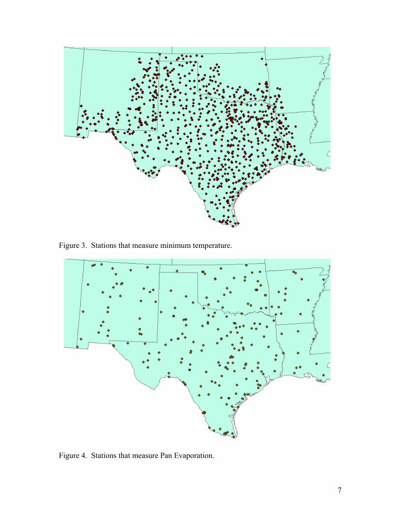
Figure 3. Stations that measure minimum temperature.
Figure 4. Stations that measure Pan Evaporation.
7

In addition to the climatic parameters from point locations, gridded estimates of
monthly and annual climatic parameters such as precipitation, maximum temperature,
minimum temperature and dew point temperature were obtained from USDA-NRCS
National Water and Climate Center’s (NWCC) PRISM climate layers. PRISM
(Parameter-elevation Regressions on Independent Slopes Model) is an interpolation
model developed by NRCS – NWCC and the Oregon State University (OSU) that uses
spatial information such as elevation, proximity to coast and other information to
interpolate the point measurements of climatic parameters. Monthly and annual data
available from most of the COOP stations have been used by the PRISM model to create
the gridded estimates. Decadal monthly and annual means of major climatic variables
from the PRISM gridded data along with decadal means for point data from a serially
complete dataset encompass the digital climatic atlas of Texas.
3.2 QA/QC of the station data
The point data obtained from NCDC had already undergone extensive QA/QC
procedures at NCDC. No additional QA/QC was performed, except to correct some
errors in the assignment of stations to particular climate divisions within Texas. Monthly
values were created from the daily data obtained from NCDC only when data for each
day of the month was available.
The monthly pan evaporation data obtain from TWDB and NCDC went through a
manual QA/QC procedure to check for data and metadata errors as there were few
stations with data and the time span of the data was shorter than with the other major
climatic parameters. The evaporation data from TWDB included data from many COOP
stations. However, the data were obtained by TWDB from those COOP stations in real
8

time prior to undergoing the standard QA/QC procedures that are followed by NCDC.
Hence, there were many inconsistencies in the TWDB dataset especially in the metadata
such as station ID, name and location. Consequently, whenever there was overlapping
data between the two sources, the NCDC data was preferred over the TWDB dataset. In
addition to these COOP stations, there are many stations across Texas that measure and
report pan evaporation to TWDB but that are not part of the COOP network and do not
submit data to NCDC. These data from TWDB were appended to the dataset from
NCDC. Further, the period of record for some of the COOP stations in TWDB is longer
and extends back to the 1940’s, whereas the data from NCDC is only available since the
1960’s. Thus, combining the data from both TWDB and NCDC resulted in a larger and
more comprehensive pan evaporation dataset.
3.3 Producing a serially complete set of station data
Historical weather data usually contain data gaps that are due to station down
times during gauge maintenance and instrumentation problems. Data gaps may also
occur during the QA/QC process when the data was flagged for inconsistency such as
data being out of reasonable range. A consistent homogenous dataset with minimal data
gaps is an essential component of the climatic atlas database. Although such a dataset
has been produced by researchers previously during the development of gridded
climatological datasets such as PRISM (Daly et al., 2002; Gibson et al., 2002; Mitchell
and Jones, 2005; Peterson et al., 1998), the data for individual stations are not available to
the public.
An essential first step in producing a serially complete set of climatic parameters
is to select a set of reference/benchmark stations that are known to be homogeneous,
9

against which target stations (COOP) can be compared (Mitchell and Jones, 2005).
Long-term records from 139 USHCN stations in Texas and neighboring states that have
undergone homogeneity corrections were selected as benchmark stations to fill the
missing data as they have already gone through a rigorous QA/QC process. The method
used for filling the missing monthly precipitation and temperature records is a modified
form of Inverse Weighting of Squared Difference (IWSD) method developed by Sun and
Peterson (2005). For each target station (COOP) - benchmark station (USHCN)
combination, 12 weights were calculated using only the months when the data for both
benchmark and target stations were available. The monthly weight is calculated as:
∑ −=
=
N
iietT
monthPP
NW
1
2argBenchmark )(
(1)
Where:
Wmonth - Weight calculated per month for each target station - benchmark station
combination
N - Number of months when both target data and benchmark data are available
PBenchmark - Monthly precipitation or temperature data for the benchmark station
PTarget - Monthly precipitation or temperature data for the target station
The larger the weight, the more similar the data are at target and benchmark
stations. In addition to the 12 monthly weights, 12 monthly biases were also calculated
for each target – benchmark station combination only for the months when the data for
both benchmark and target stations were available. For precipitation, the monthly bias
was calculated as:
10

∑
∑=
=
=N
i
N
imonth
P
PBias
1Target
1Benchmark
)(
)( (2)
For the temperature data:
N
T
N
TBias
N
i
N
imonth
∑−
∑= == 1
Target1
Benchmark )()( (3)
The process of calculating the weights and bias was iterated 139 times per target station
to combine each target station with every single benchmark station.
The benchmark stations with four highest weights for a particular month were
used to create the interpolated value for the target station. For instance, the four stations
that best correlate (highest weight) to the January data at a target station may be
completely different stations than those that best correlate with the same target station in
July. Before applying this methodology to all target (COOP) stations, test runs were
made on the 44 Texas benchmark stations (USHCN) to determine the effects of several
variables such as:
1. Effects of changing the length of the time period used to create the neighboring
station monthly weights
2. Randomly eliminating target stations,
3. Limiting neighboring station based on geographical proximity, and
4. Using more than one month to weight neighboring stations for a particular month.
The test runs showed that for both precipitation and temperature, at least 10 years
of matching data for both target and benchmark stations is needed to make reasonable
11

interpolation of the missing value at the target station. Although this limits the number of
target stations that can be used, it is necessary to maintain the integrity of the
interpolation. While no interpolation can recover the data that does not exist, research
shows that using less than ten years often produces erroneous interpolations (Figure 5).
From Figure 5, for all climatic parameters using less than 10 years of training data
increased the mean absolute error of interpolation, however increasing it beyond 10 years
did not considerably reduce the error. Further, the test runs also showed that limiting the
search for stations with four highest monthly weights from among the 20 closest
benchmark station to the target station did not increase the interpolation error
considerably (Figure 6).
Another important finding from this test run is that lower standard errors were
obtained by using more than one month to create the monthly weights. For example,
using both September and October data as opposed to using only the October data to
calculate the October monthly weights produced a more accurate result (lower standard
error). Table 2 shows the combinations of months that produced the lowest standard
error, based on tests using one, two, and three months of data. Separate evaluations were
made for East and West Texas to calculate the monthly weights for precipitation and
temperature. Only for May and August in West Texas is a single month of data optimal
for calculating the monthly weight.
12

Figure 5. Effect of the length of training period on mean absolute error of interpolation. [PRCP: Precipitation (inch); TMAX: Maximum Temperature (ºF); TMIN: Minimum Temperature (ºF)].
Figure 6. Effect of limiting the number of closest benchmark station used for interpolation on mean absolute error. [PRCP: Precipitation (inch); TMAX: Maximum Temperature (ºF); TMIN: Minimum Temperature (ºF)].
13

Table 2. Combination of months used to calculate monthly weights
Precipitation Temperature Month East
Texas West Texas
East Texas
West Texas
1 12,1 12,1 1,2 1,2 2 1,2 1,2 1,2 1,2 3 2,3 2,3 3,4 3,4 4 4,5 4,5 3,4 4,5 5 4,5 4,5 5,6 5 6 5,6,7 5,6,7 6,7 6,7 7 6,7 6,7 6,7 6,7 8 7,8 7,8 8,9 8 9 8,9 8,9,10 8,9 8,9 10 9,10 9,10 9,10 9,10 11 10,11 10,11 10,11 10,11 12 11,12 11,12 11,12 11,12
Note: Climatic divisions 1, 2, 5 and 6 belong to West Texas and rest of the six climatic divisions belongs to East Texas (See Figure 12).
Based on the procedure outlined previously and the results of the test run, missing
monthly precipitation data at target stations were filled starting from January 1890 to
December 2001. The data were filled only for those target stations with at least 10 years
of matching record with benchmark stations. Data from four benchmark stations with the
highest weights for the month from among the 20 closest stations were used to fill the
missing value at the target station. The missing values at target stations were interpolated
from the four benchmark stations as:
Interpolated value (month, year) =Wi,month ×
Value( i,month,year )
Biasi,month
⎡
⎣ ⎢
⎤
⎦ ⎥
i=1
4
∑
Wi,monthi=1
4
∑ (4)
However, when fewer than four stations were available for a particular month of
the year from among the twenty closest benchmark stations to the target station, the
process was repeated by adding the next closest station until four stations with data for a
14

particular month and year were found and used for interpolation. This process keeps
distance as an important variable but assures that four stations will be used in the
interpolation regardless of the station density near the target station. It is important to
note that the weights for individual months are calculated based on the combination of
months as listed in Table 2.
Interpolation of maximum and minimum temperature data at COOP stations was
performed as described previously for precipitation except that the bias calculated by
equation 3 is actually temperature anomaly because it is the difference in temperatures
between the benchmark and target station rather than the ratio. Hence, the equation used
to calculate missing temperature data is:
( )
∑
∑ −×=
=
=4
1,
4
1,),,(, )(
),(
imonthi
imonthiyearmonthimonthi
W
BiasValueWyearmonthvalueedInterpolat (5)
It is important to note that no attempt was made to fill the missing pan evaporation data
available from individual stations due to low station density and lack of long-term
measurements.
3.4 Generating gridded monthly precipitation, maximum and minimum temperatures
and lake evaporation coverages
3.4.1 Precipitation, maximum and minimum temperatures
High spatial resolution (4 km) monthly and annual gridded precipitation and
temperature data from 1895 to 2000 were obtained from the PRISM climatic database.
As the station density prior to 1895 was poor, monthly and gridded estimates of climatic
15

parameters were not calculated by PRISM during 1890 to 1894. The gridded PRISM
climatic dataset is the product of a multi-year multi-agency effort involving scientists
from NRCS National Water and Climate Center (NWCC) and the Oregon State
University (OSU). PRISM (Parameter-elevation Regressions on Independent Slopes
Model) is an interpolation model developed by NWCC and OSU that uses spatial
information such as elevation, proximity to coast and other information to interpolate the
point measurements of climatic parameters (Daly et al., 2002). Most of the COOP
stations were used in producing these gridded climatic layers and the base data went
through a rigorous QA/QC and data infilling procedures so that the gridded layers are of
highest quality with the best possible estimate (Johns et al., 2003).
The gridded datasets were in the Arc/Info ASCII GRID format and in the
Geographic Coordinate System encompassing the conterminous United States. Hence,
the data were clipped to the spatial extent of Texas and projected to Texas Centric
Mapping System - Albers Equal Area Conic Projection with the projection parameters
given in Table 3 as required by the Texas Administrative Code – Geographic Information
Standards. The unit of the precipitation was millimeters and the temperature was in
degrees Celsius; these were converted to inches and degrees Fahrenheit.
16

Table 3. Texas Centric Mapping System Parameters
Mapping System Name Texas Centric Mapping System/Albers Equal Area
Abbreviation TCMS/AEA Projection Albers Equal Area Conic Longitude of Origin 100 degrees West (-100) Latitude of Origin 18 degrees North (18) Lower Standard Parallel 27 degrees, 30 minutes (27.5) Upper Standard Parallel 35 degrees (35.0) False Easting 1,500,000 meters False Northing 6,000,000 meters Datum North American Datum of 1983 (NAD83) Unit of Measure meter
3.4.2 Estimation of lake evaporation
Evaporation is an important climatic and hydrologic parameter that quantifies the
amount of water lost from open water bodies due to atmospheric conditions. Due to its
nature, often evaporation is not measured directly but estimated from measurements
made using a network of Class A evaporation pans and multiplied using pan coefficients
to estimate lake evaporation. Such an estimate of evaporation is also used to infer plant
and soil evaporation for irrigation water allocation, estimating reservoir water balance,
and forecasting long-term water supply conditions, among other applications. Although
evaporation is a major component of the water budget, there is a paucity of stations that
measure evaporation. Gridded estimates of lake evaporation cannot be generated directly
from the available point measurements due to the low density of stations that measure
pan evaporation. Further, the period of record of such measurements is too short to
generate decadal monthly and annual means of lake evaporation for the entire state.
Hence, evaporation models were used along with gridded climatic layers available from
PRISM database to produce a gridded lake evaporation estimate.
17

Many evaporation models have been developed over the years to estimate
evaporation from water surfaces based on climatic parameters such as maximum and
minimum temperature, dew point temperature, solar radiation, wind speed and relative
humidity. The simple models such as the Thornthwaite method use only temperature and
the more complex models such as Penman-Monteith require inputs of almost all of the
climatic parameters mentioned previously to estimate evaporation (ASCE 1996).
However, all of these datasets are not readily available for 1890 to 2000. Hence, an
optimal balance had to found by selecting a model that computes evaporation with
reasonable accuracy using limited climatic data.
The aerodynamic method is one of the widely used procedures for estimating
evaporation from lakes and large reservoirs. The model was originally developed by U.S.
Geological Survey in the 1950’s (ASCE 1996):
zzs ueeME )( −= (6)
where E is the evaporation in mm per day, M is the mass transfer coefficient, es is the
saturation vapor pressure at the surface water temperature Ts (kPa), ez is the vapor
pressure of the air at height z (kPa) and uz is the wind velocity at level z in m/s. Although
direct measurements of saturated vapor pressure (es) and actual vapor pressure (ez) were
not available, they can be calculated from maximum, minimum, and dew point
temperatures. The saturation vapor pressure and actual vapor pressure were calculated as
follows (Allen et al., 1998):
⎥⎦⎤
⎢⎣⎡
+=
3.23727.17exp6108.0)(
TTTe (7)
18

2)()( min
0max
0 TeTees
+= (8)
⎥⎦
⎤⎢⎣
⎡+
=3.237
27.17exp6108.0
dew
dewz T
Te (9)
Where: e(T) is saturation vapor pressure at the air temperature T (kPa), T air temperature
(°C).
All the temperature data were readily available in the gridded format from the
PRISM dataset. Monthly and annual dew point temperature from 1895 to 2000 were
obtained from the PRISM database and processed using the same procedures described in
section 3.4.1.
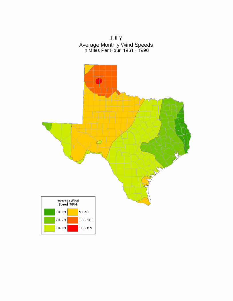
However, long term wind speed data were not available since wind speed is
measured at a limited number of stations. Based on the longest available records of wind
speed between 1961 and 1990, contour maps of monthly and annual average wind speed
were available from the NCDC CLIMAPS dataset. However, the contours are widely
spaced and each represents an average wind speed increment of one mile per hour and
range in value between 6 miles per hour to 12 miles per hour. Hence, these contour lines
were interpolated between lines to get a fine breakdown of intermediate values so that the
output evaporation grid will be smooth.
The mass transfer coefficient M is calculated as (ASCE 1996):
Ea C
PM
ρ53740= (10)
Where ρa is the density of air (kg m-3)), P is the atmospheric pressure (kPa) and CE is the
bulk evaporation coefficient (0.0015). Atmospheric pressure was calculated based on
19

elevation from the digital elevation model using the simplified form of the gas law for a
standard atmosphere (Allen et al., 1998):
26.5
2930065.02933.101 ⎟
⎠⎞
⎜⎝⎛ −
=zP (11)
Where, z is the elevation above mean sea level (m). The air density was calculated from
pressure and temperature as (ASCE 1996):
RTP
va
1000=ρ (12)
Pe
TTz
v378.01−
= (13)
Where, R is the specific gas constant for dry air, 287 J/kg/K, Tv is the virtual temperature
(K), ez is the actual vapor pressure (kPa) and P is atmospheric pressure (kPa).
3.4.3 Correction of lake evaporation
The evaporation estimated using the aerodynamic method described above should
be adjusted based on measured pan evaporation and multiplied by a pan coefficient for
estimating lake evaporation. Best estimates of monthly evaporation with at least five
years of data during a 30 year period from 1971 to 2000 were available for about 94
stations out of the 232 stations that measure evaporation (Figure 7).
The evaporation estimated using the aerodynamic method was compared with the
monthly measurements at these 94 evaporation stations from 1971 to 2000 and an
evaporation ratio (ER) was estimated for each month the measurement was available as:
ER = measured evaporation / model evaporation (14)
20

Based on the ER calculated for at least 5 years for each month during the 30 year period,
monthly average evaporation ratio was estimated for each of the 94 stations. These
estimates of ER where then used to estimate lake evaporation as:
Lake evaporation = model evaporation X ER X pan coefficient
Monthly pan coefficients were available for each one degree quadrangle across Texas and
were based on the Evaporation Atlas of the United States (Farnsworth et al., 1982).
Figure 7. Evaporation stations with at least five years of data from 1971-2000.
Monthly pan coefficients were assigned to each of the 94 evaporation stations
based on the quadrangles in which they lie. These pan coefficients were then multiplied
with the 30-year average evaporation ratio described earlier. The product of pan
coefficients and ER for individual stations was then spatially interpolated using
regularized spline technique across the entire state for each month. The average of these
21

twelve monthly grids was calculated to obtain the average annual correction grid. These
interpolated correction grids were then multiplied with the model evaporation grid
calculated for each month from 1895 to 2000 to produce gridded lake evaporation grids.
3.5 Verifying the gridded PRISM climatic data
The PRISM climatic data layers were calculated using sophisticated interpolation
techniques that incorporates a conceptual framework which addresses the spatial scale
and pattern of orographic precipitation and temperature using information such as
elevation, proximity to coast, and other information to interpolate the point measurements
of climatic parameters (Daly et al., 2002). As most of the COOP stations were already
used in the creation of this gridded data set, it is difficult to assess the accuracy of PRISM
grids. Independent weather stations that are not part of the COOP network and that do
not report to NCDC were available only at very few locations such as in the North Texas
High Plains Evapotranspiration Network of the Texas Agricultural Experiment Station
(http://amarillo2.tamu.edu/nppet/petnet1.htm) (Figure 8).
22

Figure 8. North Texas High Plains ET network stations along with the COOP stations.
There are 16 weather stations that are part of the High Plains ET network that
measure precipitation, maximum and minimum temperature on a daily basis. The daily
values for these climatic parameters were available for a 5 year period from 1996 to 2000
for most of the 16 stations. Monthly means of these climatic parameters where calculated
for these 16 stations for the 5 year period and compared with the PRISM grids to verify
their accuracy. The average difference in monthly precipitation for the 5 year period for
the 16 stations was about 0.25 inches for an average monthly rainfall of 2.26 inches
(Figure 9) and average difference in temperature was within 0.4 and 0.7 degree
Fahrenheit for minimum and maximum temperatures respectively (Figure 10).
23

Figure 9. Difference in monthly precipitation between PRISM grids and the High Plains ET network stations.
Figure 10. Difference in monthly temperature between PRISM grids and the High Plains ET network stations.
24

It was interesting to note that at most of the High Plain stations the temperatures were
below the PRISM gridded estimates. This is probably because most of the COOP
stations are located close to urban occupation where the temperature could be slightly
higher than the surrounding area due to radiation from asphalt and concrete in urban
structures.
Based on the COOP station density in the Texas High Plains (Figure 8) and
comparing it with the density of COOP network for the rest of Texas (Figure 1, 2, 3) we
can infer that the error in PRISM grids might be high in the west Texas Trans Pecos
region due to comparatively low station density and high differences in topography. In
the Rolling Plains, Edward Plateau and south Texas the errors in PRISM grids should be
similar to that of High Plains due to similar station densities. In Central and East Texas
regions the error in PRISM grids could be lower than that of High Plains due to the
higher station density. While it is imperative to understand that no interpolation
technique can duplicate the exact measurements, these errors are well within the
acceptable range for the purpose of creating long-term decadal means of gridded climatic
parameters.
3.6 Calculating monthly and annual decadal means of gridded and point climatic data
The gridded and point climate data consisting of monthly and annual
precipitation, maximum and minimum temperature and evaporation were generated based
on the data available from various sources ranging from 1890 to 2000. Then decadal
monthly and annual means for each climatic parameter were calculated for the 11
decades. With the exception of measured pan evaporation, the decadal statistics for most
of the stations were available for all the 11 decades. However, gridded evaporation
25

produced using the methodology described in Section 3.4.2 were used to calculate grids
of decadal monthly and annual means of lake evaporation. It is important to note that for
the decade of 1891 to 1900, only six years of gridded data from 1895 to 1900 were
available from the PRISM database for calculating the decadal statistics. In addition to
the decadal statistics, 30 year (1971-2000) monthly and annual means were also
calculated for each climatic parameter and included in the database.
3.7 Creating an ArcGIS geodatabase containing gridded and a database containing
point monthly and annual decadal means of climatic parameters.
The gridded monthly and annual decadal means of climatic parameters were
imported into an ArcGIS geodatabase. The advantage of using a geodatabase is that the
data can be easily queried, displayed, analyzed and the integrity of the dataset can be
maintained while allowing efficient storage and distribution of this large dataset. In
addition to this gridded geodatabase of climatic parameters, the decadal statistics of
climatic parameters for the individual stations were included in a complementary
database. This database can be used to query hundreds of weather stations for data on
any particular decade, month, or station. The 30-year monthly and annual climatic
statistics were also mapped into layouts along with contour lines following a similar
pattern as that of the earlier climatic atlas (Appendix A).
4.0 Dividing Texas into smaller climatic divisions
The 1983 climatic atlas (LP192) described Texas as having three major climatic
types which are classified as Continental, Mountain, and Modified Marine. The
Modified Marine was further sub-classified into four “Subtropical” zones (Figure 11).
26

Subsequently NCDC divided Texas into ten climatic zones of homogenous climatic
patterns based on statistical analysis. The regions were made to coincide with political
Figure 11. Texas climatic types (LP192- 1983 climatic atlas).
27

Figure 12. NCDC climatic divisions
boundaries (Figure 12) for issuing warnings and forecasts of climatic events such as
drought. However, there is a growing concern among the action agencies responsible for
drought monitoring and response that these climatic divisions are rather too large to be of
use for providing information on local impacts. The gridded climatic layers produced in
this study are of immense use for identifying climatic divisions of varying sizes based on
an agencies’ requirements.
Thirty year monthly means (1971-2000) of precipitation, maximum and minimum
temperature, dew point temperature and mean monthly wind speed (60 data layers) were
used to identify unique climatic zones of varying size across Texas. In order to identify
the unique climatic zones, each climatic parameter was normalized using the maximum
and minimum values of the climatic parameters to make sure that the resultant data layer
28

was unit less. Using these 60 layers of information the Iterative Self-Organizing Data
Analysis Technique (ISODATA) (Tou and Gonzalez, 1974) was used to find clusters
with unique climatic properties. This clustering algorithm identifies unique patterns of
temporal variations in the five climatic parameters and then assigns each pixel to a unique
class iteratively until about 95% of the pixel does not change classes within subsequent
iterations. The procedure was used to classify Texas into 5, 10, 25 and 50 different
climatic classes. Appendix B contain illustrations of these climatic divisions along with
an overlay of the NCDC’s 10 climatic division (image on the left) along with the new
climatic division boundaries corrected to align with county political boundaries (image
on the right) based on the dominant climatic zone of the county. It is interesting to note
that the 10 climatic zones produced by ISODATA are different from the current NCDC
climatic divisions, except for the High-Plains climatic division. The area of the smallest
and largest climatic divisions created from this procedure are given in Table 4.
Table 4. Area of climatic divisions produced by varying the number of unique climatic
classes.
No. of classes
Smallest Area Sq.mi
Largest Area Sq.mi
Average Area Sq.mi
5 41,347 68,912 54,777 10 19,367 35,330 27,389 25 5,622 16,074 10,955 50 500 11,577 5,478
NCDC* 3,044 38,761 26,410 * NCDC 10 climatic divisions
5.0 Conclusions
The current work developed and assembled the best possible data to produce
gridded and point decadal monthly and annual statistics for 11 decades since 1890. This
29

rich data source will be of immense benefit to the wider community of Texas in better
understanding the spatial and temporal climatic variability across the state. It is our hope
that the digital database will significantly improve the decision making process during the
analysis, and planning phases of major water resources projects across Texas.
30

Reference:
Allen, R. G., L. S. Pereira, D. Raes, and M. Smith. 1998. Crop Evapotranspiration: Guidelines for computing crop water requirements. FAO Irrigation and Drainage Paper No.56. Rome, Italy: FAO.
ASCE. 1996. Evaporation and Transpiration. In Hydrology Handbook, 125-181. ASCE Manuals and Reports on Engineering Practice No. 28.
Daly, C., W. P. Gibson, G. H. Taylor, G. L. Johnson, and P. Pasteris. 2002. A knowledge-based approach to the statistical mapping of climate, Climate Research, 22 (2): 99-113.
Gibson, W.P., C. Daly, D. Kittel, D. Nychka, C. Johns, N. Rosenbloom, A. McNab, and G. Taylor. 2002. Development of a 103-year high-resolution climate data set for the conterminous United States, in 13th AMS Conference on Applied Climatology, pp. 181-183, Portland, OR.
Johns, C. J., D. Nychka, T. G. F. Kittel, C. Daly. 2003. Infilling sparse records of spatial fields. Journal of the American Statistical Association, 98 (464): 796-806.
Larkin, T. J., and G. W. Bomar. 1983. Climatic Atlas of Texas. Texas Dept. of Water Resources. LP-192. Austin, Texas. 151p.
Mitchell, T. D., and P. D. Jones. 2005. An improved method of constructing a database of monthly climate observations and associated high-resolution grids, International Journal of Climatology, 26: 693-712.
Farnsworth, R.K., E.S. Thompson, and E.L. Peck (1982). Evaporation Atlas for the Contiguous 48 United States. NOAA Technical Report NWS 33, Washington, D.C.
Peterson, T.C., D. Easterling, T. Karl, P.Y. Groisman, N. Nicholls, N. Plummer, S. Torok, I. Auer, R. Boehm, D. Gullet, L. Vincent, R. Heino, H. Tuomenvirta, O. Mestre, T. Szentimrey, J. Salinger, E. J. Forland, I. Hanssen-Bauer, H. Alexandersson, P. Jones, and D. Parker. 1998. Homogeneity adjustments of in situ atmospheric climate data: A review, International Journal of Climatology, 18: 1493-1517.
Sun, B., and T. C. Peterson. 2005. Estimating temperature normals for USCRN stations. International Journal of Climatology, 25 (14): 1809-1817.
Tou, J. T., and R. C. Gonzalez. 1974. Pattern Recognition Principles. Reading, Massachusetts: Addison-Wesley Publishing Company.
31

Appendix A
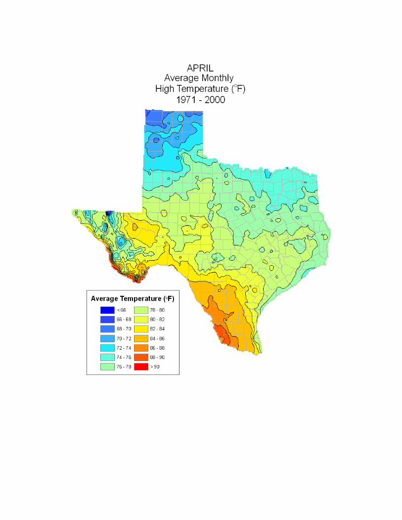
In the following section, 30 year (1971-2000) monthly and annual means of precipitation,
maximum temperature, minimum temperature and lake evaporation are mapped into
layouts along with contour lines following a similar pattern as that of the earlier climatic
atlas LP 192. Decadal monthly and annual means of precipitation, maximum
temperature, minimum temperature and lake evaporation for each decade from 1890 to
2000 are available in the ESRI Geodatabase format in the attached DVD.

Average Monthly Precipitation Maps


Average Monthly Maximum Temperature Maps


Average Monthly Minimum Temperature Maps


Average Monthly Lake Evaporation Maps


Average Monthly Wind Speed Maps
Based on the longest available records of wind speed between 1961 and 1990, contour
maps of monthly and annual average wind speed were available from the NCDC
CLIMAPS dataset (http://cdo.ncdc.noaa.gov/cgi-bin/climaps/climaps.pl). These contour
maps were clipped for Texas and reproduced in this section.


Appendix B
Thirty year monthly means (1971-2000) of precipitation, maximum and minimum
temperature, dew point temperature and mean monthly wind speed (60 data layers) were
used to identify unique climatic zones of varying size across Texas. In order to identify
the unique climatic zones, each climatic parameter was normalized using the maximum
and minimum values of the climatic parameters to make sure that the resultant data layer
was unit less. Using these 60 layers of information the Iterative Self-Organizing Data
Analysis Technique (ISODATA) (Tou and Gonzalez, 1974) was used to find clusters
with unique climatic properties. This clustering algorithm identifies unique patterns of
temporal variations in the five climatic parameters and then assigns each pixel to a unique
class iteratively until about 95% of the pixel does not change classes within subsequent
iterations. The procedure was used to classify Texas into 5, 10, 25 and 50 different
climatic classes. Appendix B contain illustrations of these climatic divisions along with
an overlay of the NCDC’s 10 climatic division (image on the left) along with the new
climatic division boundaries corrected to align with county political boundaries (image
on the right) based on the dominant climatic zone of the county. It is interesting to note
that the 10 climatic zones produced by ISODATA are different from the current NCDC
climatic divisions, except for the High-Plains climatic division.

Note: New climatic divisions along with an overlay of the NCDC’s 10 climatic division boundary (Figure 12)

Note: New climatic divisions along with an overlay of the NCDC’s 10 climatic division boundary (Figure 12)

Note: New climatic divisions along with an overlay of the NCDC’s 10 climatic division boundary (Figure 12)

Note: New climatic divisions along with an overlay of the NCDC’s 10 climatic division boundary (Figure 12)


![Texas - Climatic Atlas of Texas, 1983 [pdf format] · PDF fileClimatic Atlas of Texas LP-192 TEXAS DEPARTMENT OF WATER RESOURCES ... whereas the wind roses are based upon approximate](https://static.fdocuments.in/doc/165x107/5a78f9ca7f8b9a217b8b8618/texas-climatic-atlas-of-texas-1983-pdf-format-atlas-of-texas-lp-192-texas-department.jpg)