1

Washington University in St. Louis

School of Engineering and Applied Science

Electrical and Systems Engineering Department

ESE498

Digital Active Noise Cancelling

Headphones

By

Michael Jezierny

Brenton Keller

Kyung Yul Lee

Supervisor

Prof. Robert Morley

Submitted in Partial Fulfillment of the Requirement for the BSEE Degree,

Electrical and Systems Engineering Department, School of Engineering and

Applied Science,

Washington University in St. Louis

May 2010

2

Table of Contents

Student Statement, Project Abstract, Acknowledgement…4

Problem Formulation...4

Project Specifications…5

Concept synthesis

Literature Review…5-7

Concept Generation and Reduction…8

Detailed Engineering Analysis and Design Presentation…9-22

Cost Analysis…23

Hazards and Failure Analysis…23

Conclusions…23

References…24-25

3

List of Figures and Tables

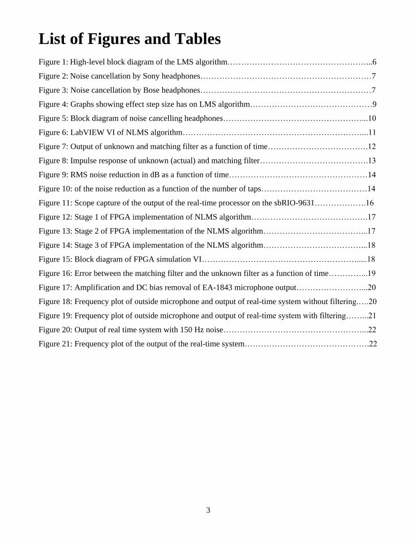
Figure 1: High-level block diagram of the LMS algorithm……………………………………………...6

Figure 2: Noise cancellation by Sony headphones………………………………………………………7

Figure 3: Noise cancellation by Bose headphones………………………………………………………7

Figure 4: Graphs showing effect step size has on LMS algorithm………………………………………9

Figure 5: Block diagram of noise cancelling headphones……………………………………………...10

Figure 6: LabVIEW VI of NLMS algorithm…………………………………………………………...11

Figure 7: Output of unknown and matching filter as a function of time……………………………….12

Figure 8: Impulse response of unknown (actual) and matching filter………………………………….13

Figure 9: RMS noise reduction in dB as a function of time……………………………………………14

Figure 10: of the noise reduction as a function of the number of taps…………………………………14

Figure 11: Scope capture of the output of the real-time processor on the sbRIO-9631……………….16

Figure 12: Stage 1 of FPGA implementation of NLMS algorithm…………………………………….17

Figure 13: Stage 2 of FPGA implementation of the NLMS algorithm………………………………...17

Figure 14: Stage 3 of FPGA implementation of the NLMS algorithm………………………………...18

Figure 15: Block diagram of FPGA simulation VI………………………………………………….....18

Figure 16: Error between the matching filter and the unknown filter as a function of time…………...19

Figure 17: Amplification and DC bias removal of EA-1843 microphone output……………………...20

Figure 18: Frequency plot of outside microphone and output of real-time system without filtering.….20

Figure 19: Frequency plot of outside microphone and output of real-time system with filtering……...21

Figure 20: Output of real time system with 150 Hz noise……………………………………………...22

Figure 21: Frequency plot of the output of the real-time system……………………………………….22

4

Student Statement

We affirm that we have applied ethics to the design process and in the selection of the final proposed

design.

Project Abstract

In this project, we tried to build noise-cancelling headphones using a two microphone system, one

microphone to sample the ambient noise and another to detect how well the noise cancelation is

working. We used a finite impulse response (FIR) matching filter to model a system with an unknown

transfer characteristic. Then, the output of the matching filter is inverted to create the anti-noise, which

is combined electrically with the music and played into the headphones. We simulated our project

LabVIEW 8.6 and used LabVIEW Robotics 2009 to implement a real-time system.

Acknowledgement

We would like to thank both Prof. Morley and Ed Richter to help us finish this senior project.

Problem Formulation

We all have trouble listening to music when we are surrounded by noise. For example, it is very

difficult to listen to music on an airplane because of its engine noise. However, we all want to enjoy

our music whenever, wherever. This motivated us to make noise-cancelling headphones that reduce

unwanted ambient sounds.

In order to design the noise-cancelling headphones, we first had to do some research on it. We tried to

find articles and patents about the noise-cancelling headphones. After we had done some research, we

had to decide how we were going to set up so that we can simulate our algorithm and matching filters.

We agreed on using a programming language called LabVIEW. In LabVIEW, we tried to simulate the

finite impulse response (FIR) matching filter by using both the least-mean-squares (LMS) and the

normalized-least-mean-squares (NLMS) algorithm. Then, we kept designing to try and make it work in

real time to solve our problem.

5

Project Specifications

Our goal in this project was to find a noise-cancellation algorithm and to implement it in hardware; that

is, on a pair of non-noise-cancelling headphones. Due to the nature of the project, we did not designate

a target level of noise reduction for our algorithm. Instead, our goal was simply to maximize the

performance of our algorithm, subject to the constraint that it be readily implementable in hardware.

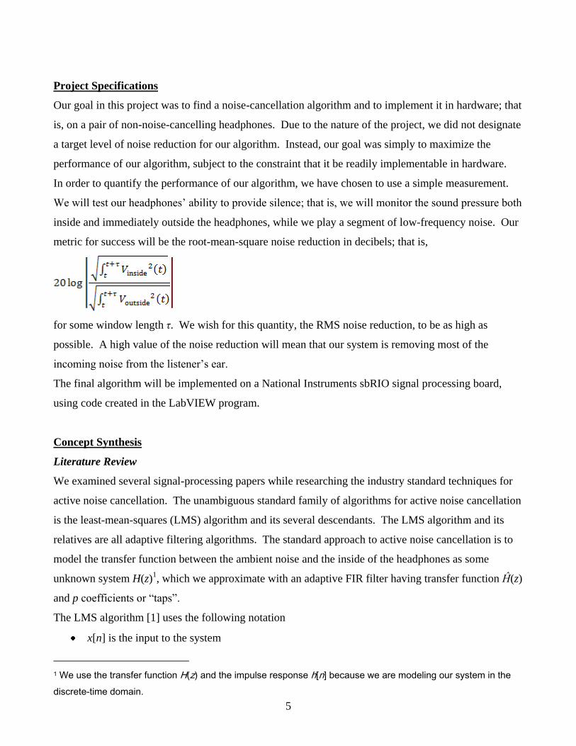
In order to quantify the performance of our algorithm, we have chosen to use a simple measurement.

We will test our headphones’ ability to provide silence; that is, we will monitor the sound pressure both

inside and immediately outside the headphones, while we play a segment of low-frequency noise. Our

metric for success will be the root-mean-square noise reduction in decibels; that is,

for some window length τ. We wish for this quantity, the RMS noise reduction, to be as high as

possible. A high value of the noise reduction will mean that our system is removing most of the

incoming noise from the listener’s ear.

The final algorithm will be implemented on a National Instruments sbRIO signal processing board,

using code created in the LabVIEW program.

Concept Synthesis

Literature Review

We examined several signal-processing papers while researching the industry standard techniques for

active noise cancellation. The unambiguous standard family of algorithms for active noise cancellation

is the least-mean-squares (LMS) algorithm and its several descendants. The LMS algorithm and its

relatives are all adaptive filtering algorithms. The standard approach to active noise cancellation is to

model the transfer function between the ambient noise and the inside of the headphones as some

unknown system H(z)1, which we approximate with an adaptive FIR filter having transfer function Ĥ(z)

and p coefficients or “taps”.

The LMS algorithm [1] uses the following notation

x[n] is the input to the system

1 We use the transfer function H(z) and the impulse response h[n] because we are modeling our system in the

discrete-time domain.

6

y[n] is the output of the unknown system H(z)

ŷ[n] is the output of the adaptive filter Ĥ(z)

x[n] is a vector of the last p values of x[n]

ĥ[n] is the vector of FIR coefficients for Ĥ(z), at the nth simulation step

v[n] is the interference

d[n] = y[n] + v[n]

e[n] = d[n] − ŷ[n]

µ is the “step size” or “learning rate”

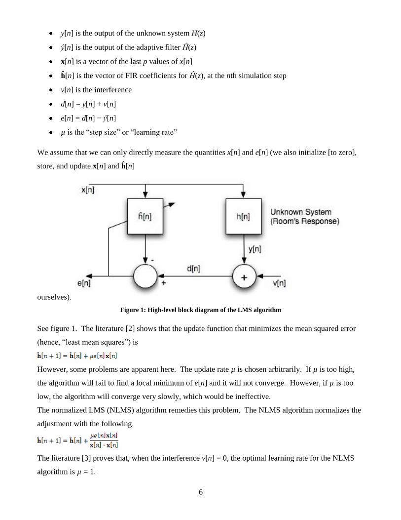
We assume that we can only directly measure the quantities x[n] and e[n] (we also initialize [to zero],

store, and update x[n] and ĥ[n]

ourselves).

Figure 1: High-level block diagram of the LMS algorithm

See figure 1. The literature [2] shows that the update function that minimizes the mean squared error

(hence, “least mean squares”) is

However, some problems are apparent here. The update rate µ is chosen arbitrarily. If µ is too high,

the algorithm will fail to find a local minimum of e[n] and it will not converge. However, if µ is too

low, the algorithm will converge very slowly, which would be ineffective.

The normalized LMS (NLMS) algorithm remedies this problem. The NLMS algorithm normalizes the

adjustment with the following.

The literature [3] proves that, when the interference v[n] = 0, the optimal learning rate for the NLMS

algorithm is µ = 1.

7

The literature revealed some more exotic methods. For example, some complex noise-cancellation

algorithms use only one sensor, but can still approximate the noise [3]. Other researchers suggested

variations on the popular LMS algorithm, such as a frequency-divided sub-band FXLMS/FXNLMS

algorithm [3], and the MMLMS algorithm which includes delay compensation and back-propagation

learning techniques borrowed from artificial neural networks [10].

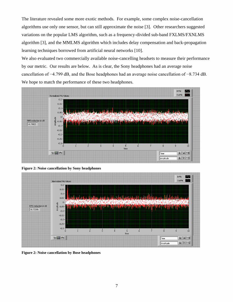
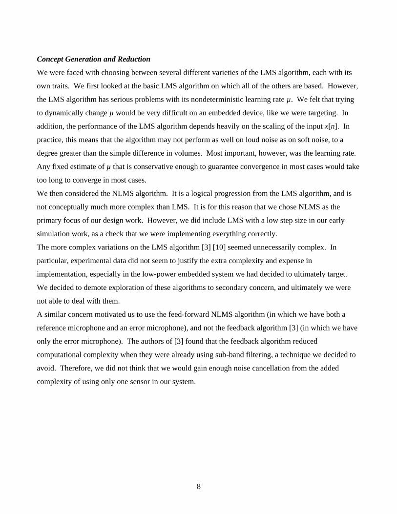
We also evaluated two commercially available noise-cancelling headsets to measure their performance

by our metric. Our results are below. As is clear, the Sony headphones had an average noise

cancellation of −4.799 dB, and the Bose headphones had an average noise cancellation of −8.734 dB.

We hope to match the performance of these two headphones.

Figure 2: Noise cancellation by Sony headphones

Figure 2: Noise cancellation by Bose headphones

8

Concept Generation and Reduction

We were faced with choosing between several different varieties of the LMS algorithm, each with its

own traits. We first looked at the basic LMS algorithm on which all of the others are based. However,

the LMS algorithm has serious problems with its nondeterministic learning rate µ. We felt that trying

to dynamically change µ would be very difficult on an embedded device, like we were targeting. In

addition, the performance of the LMS algorithm depends heavily on the scaling of the input x[n]. In

practice, this means that the algorithm may not perform as well on loud noise as on soft noise, to a

degree greater than the simple difference in volumes. Most important, however, was the learning rate.

Any fixed estimate of µ that is conservative enough to guarantee convergence in most cases would take

too long to converge in most cases.

We then considered the NLMS algorithm. It is a logical progression from the LMS algorithm, and is

not conceptually much more complex than LMS. It is for this reason that we chose NLMS as the

primary focus of our design work. However, we did include LMS with a low step size in our early

simulation work, as a check that we were implementing everything correctly.

The more complex variations on the LMS algorithm [3] [10] seemed unnecessarily complex. In

particular, experimental data did not seem to justify the extra complexity and expense in

implementation, especially in the low-power embedded system we had decided to ultimately target.

We decided to demote exploration of these algorithms to secondary concern, and ultimately we were

not able to deal with them.

A similar concern motivated us to use the feed-forward NLMS algorithm (in which we have both a

reference microphone and an error microphone), and not the feedback algorithm [3] (in which we have

only the error microphone). The authors of [3] found that the feedback algorithm reduced

computational complexity when they were already using sub-band filtering, a technique we decided to

avoid. Therefore, we did not think that we would gain enough noise cancellation from the added

complexity of using only one sensor in our system.

9

Detailed Engineering Analysis and Design Presentation

The first step in our design process was to model the system we would create. In the modeling process

we had two major decisions to make. The first decision was how many microphones we would use in

our system. In some commercial noise-cancelling headphones 2 microphones are used [8], while some

research has been done where only 1 microphone was used [5]. [5] presents a case for using a two

microphone system and shows that with that approach he was able to achieve 3 dB better noise

reduction than a system with one microphone. We decided to model our system after [5].

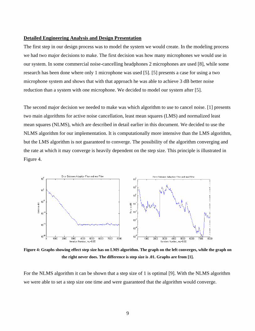
The second major decision we needed to make was which algorithm to use to cancel noise. [1] presents

two main algorithms for active noise cancellation, least mean squares (LMS) and normalized least

mean squares (NLMS), which are described in detail earlier in this document. We decided to use the

NLMS algorithm for our implementation. It is computationally more intensive than the LMS algorithm,

but the LMS algorithm is not guaranteed to converge. The possibility of the algorithm converging and

the rate at which it may converge is heavily dependent on the step size. This principle is illustrated in

Figure 4.

Figure 4: Graphs showing effect step size has on LMS algorithm. The graph on the left converges, while the graph on

the right never does. The difference is step size is .01. Graphs are from [1].

For the NLMS algorithm it can be shown that a step size of 1 is optimal [9]. With the NLMS algorithm

we were able to set a step size one time and were guaranteed that the algorithm would converge.

10

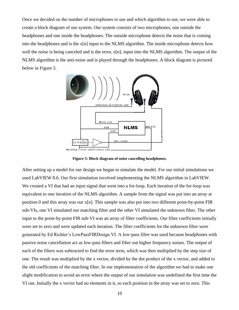
Once we decided on the number of microphones to use and which algorithm to use, we were able to

create a block diagram of our system. Our system consists of two microphones, one outside the

headphones and one inside the headphones. The outside microphone detects the noise that is coming

into the headphones and is the x[n] input to the NLMS algorithm. The inside microphone detects how

well the noise is being canceled and is the error, e[n], input into the NLMS algorithm. The output of the

NLMS algorithm is the anti-noise and is played through the headphones. A block diagram is pictured

below in Figure 5.

Figure 5: Block diagram of noise cancelling headphones.

After setting up a model for our design we began to simulate the model. For our initial simulations we

used LabVIEW 8.6. Our first simulation involved implementing the NLMS algorithm in LabVIEW.

We created a VI that had an input signal that went into a for-loop. Each iteration of the for-loop was

equivalent to one iteration of the NLMS algorithm. A sample from the signal was put into an array at

position 0 and this array was our x[n]. This sample was also put into two different point-by-point FIR

sub-VIs, one VI simulated our matching filter and the other VI simulated the unknown filter. The other

input to the point-by-point FIR sub-VI was an array of filter coefficients. Our filter coefficients initially

were set to zero and were updated each iteration. The filter coefficients for the unknown filter were

generated by Ed Richter’s LowPassFIRDesign VI. A low-pass filter was used because headphones with

passive noise cancellation act as low-pass filters and filter out higher frequency noises. The output of

each of the filters was subtracted to find the error term, which was then multiplied by the step size of

one. The result was multiplied by the x vector, divided by the dot product of the x vector, and added to

the old coefficients of the matching filter. In our implementation of the algorithm we had to make one

slight modification to avoid an error where the output of our simulation was undefined the first time the

VI ran. Initially the x vector had no elements in it, so each position in the array was set to zero. This

11

caused a divided by zero error when e[n]*x[n]*µ was divided by the dot product of x. When this

happened the output of our matching filter was always not a number (NAN) for the first execution of

the VI after it compiled. To fix this problem we set all of the positions in the x array to 1*10-6

. This

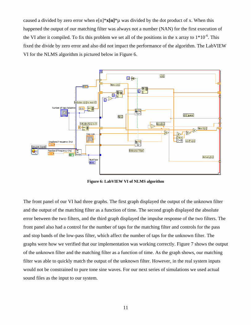
fixed the divide by zero error and also did not impact the performance of the algorithm. The LabVIEW

VI for the NLMS algorithm is pictured below in Figure 6.

Figure 6: LabVIEW VI of NLMS algorithm

The front panel of our VI had three graphs. The first graph displayed the output of the unknown filter

and the output of the matching filter as a function of time. The second graph displayed the absolute

error between the two filters, and the third graph displayed the impulse response of the two filters. The

front panel also had a control for the number of taps for the matching filter and controls for the pass

and stop bands of the low-pass filter, which affect the number of taps for the unknown filter. The

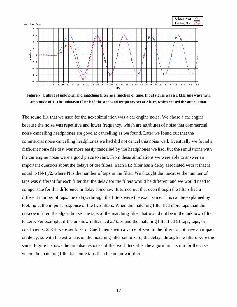
graphs were how we verified that our implementation was working correctly. Figure 7 shows the output

of the unknown filter and the matching filter as a function of time. As the graph shows, our matching

filter was able to quickly match the output of the unknown filter. However, in the real system inputs

would not be constrained to pure tone sine waves. For our next series of simulations we used actual

sound files as the input to our system.

12

Figure 7: Output of unknown and matching filter as a function of time. Input signal was a 1 kHz sine wave with

amplitude of 1. The unknown filter had the stopband frequency set at 2 kHz, which caused the attenuation.

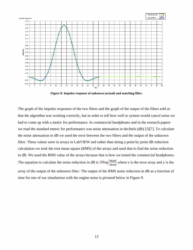
The sound file that we used for the next simulation was a car engine noise. We chose a car engine

because the noise was repetitive and lower frequency, which are attributes of noise that commercial

noise cancelling headphones are good at cancelling as we found. Later we found out that the

commercial noise cancelling headphones we had did not cancel this noise well. Eventually we found a

different noise file that was more easily cancelled by the headphones we had, but the simulations with

the car engine noise were a good place to start. From these simulations we were able to answer an

important question about the delays of the filters. Each FIR filter has a delay associated with it that is

equal to (N-1)/2, where N is the number of taps in the filter. We thought that because the number of

taps was different for each filter that the delay for the filters would be different and we would need to

compensate for this difference in delay somehow. It turned out that even though the filters had a

different number of taps, the delays through the filters were the exact same. This can be explained by

looking at the impulse response of the two filters. When the matching filter had more taps than the

unknown filter, the algorithm set the taps of the matching filter that would not be in the unknown filter

to zero. For example, if the unknown filter had 27 taps and the matching filter had 51 taps, taps, or

coefficients, 28-51 were set to zero. Coefficients with a value of zero in the filter do not have an impact

on delay, so with the extra taps on the matching filter set to zero, the delays through the filters were the

same. Figure 8 shows the impulse response of the two filters after the algorithm has run for the case

where the matching filter has more taps than the unknown filter.

13

Figure 8: Impulse response of unknown (actual) and matching filter.

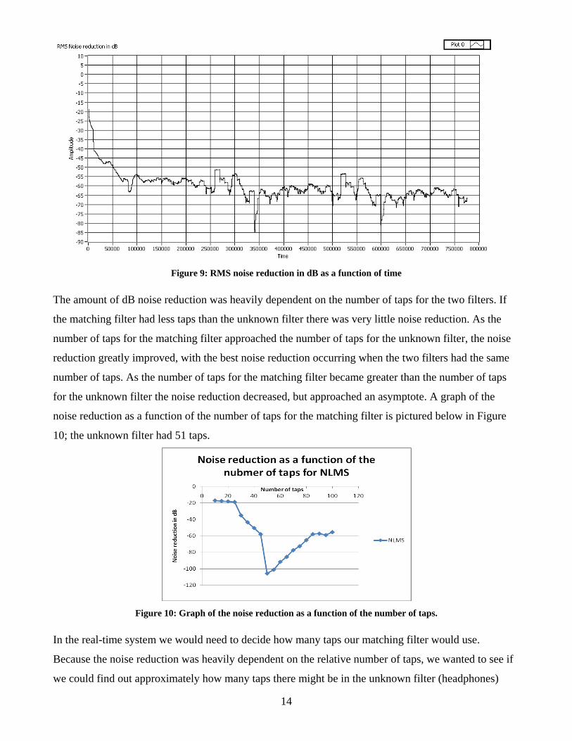
The graph of the impulse responses of the two filters and the graph of the output of the filters told us

that the algorithm was working correctly, but in order to tell how well or system would cancel noise we

had to come up with a metric for performance. In commercial headphones and in the research papers

we read the standard metric for performance was noise attenuation in decibels (dB) [5][7]. To calculate

the noise attenuation in dB we used the error between the two filters and the output of the unknown

filter. These values were in arrays in LabVIEW and rather than doing a point by point dB reduction

calculation we took the root mean square (RMS) of the arrays and used that to find the noise reduction

in dB. We used the RMS value of the arrays because that is how we tested the commercial headphones.

The equation to calculate the noise reduction in dB is where e is the error array and y is the

array of the output of the unknown filter. The output of the RMS noise reduction in dB as a function of

time for one of our simulations with the engine noise is pictured below in Figure 9.

14

Figure 9: RMS noise reduction in dB as a function of time

The amount of dB noise reduction was heavily dependent on the number of taps for the two filters. If

the matching filter had less taps than the unknown filter there was very little noise reduction. As the

number of taps for the matching filter approached the number of taps for the unknown filter, the noise

reduction greatly improved, with the best noise reduction occurring when the two filters had the same

number of taps. As the number of taps for the matching filter became greater than the number of taps

for the unknown filter the noise reduction decreased, but approached an asymptote. A graph of the

noise reduction as a function of the number of taps for the matching filter is pictured below in Figure

10; the unknown filter had 51 taps.

Figure 10: Graph of the noise reduction as a function of the number of taps.

In the real-time system we would need to decide how many taps our matching filter would use.

Because the noise reduction was heavily dependent on the relative number of taps, we wanted to see if

we could find out approximately how many taps there might be in the unknown filter (headphones)

15

based on the delay from the outside of the headphones to the inside of the headphones. We set up a test

to try and see if there was any delay from the time a microphone outside the headphones picked up a

signal to the time a microphone inside the headphones picked up a signal. We found out that there was

almost no discernable delay with the tools we used, not surprising given the speed of sound, and were

not able to get a better idea of how many taps the unknown filter might have.

To demonstrate how our system would ideally work we added in music to our simulation. The music

was added to the difference between the matching and unknown filters, played out through the sound

card and written to a file. On the front panel we added a switch that gave the option of cancelling the

noise.

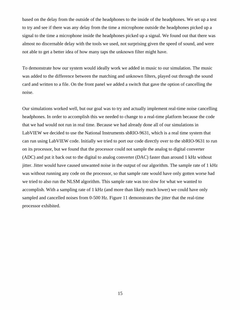
Our simulations worked well, but our goal was to try and actually implement real-time noise cancelling

headphones. In order to accomplish this we needed to change to a real-time platform because the code

that we had would not run in real time. Because we had already done all of our simulations in

LabVIEW we decided to use the National Instruments sbRIO-9631, which is a real time system that

can run using LabVIEW code. Initially we tried to port our code directly over to the sbRIO-9631 to run

on its processor, but we found that the processor could not sample the analog to digital converter

(ADC) and put it back out to the digital to analog converter (DAC) faster than around 1 kHz without

jitter. Jitter would have caused unwanted noise in the output of our algorithm. The sample rate of 1 kHz

was without running any code on the processor, so that sample rate would have only gotten worse had

we tried to also run the NLSM algorithm. This sample rate was too slow for what we wanted to

accomplish. With a sampling rate of 1 kHz (and more than likely much lower) we could have only

sampled and cancelled noises from 0-500 Hz. Figure 11 demonstrates the jitter that the real-time

processor exhibited.

16

Figure 11: Scope capture of the output of the real-time processor on the sbRIO-9631. The sample rate was set to 4

kHz and the input was a 500 Hz square wave. The first capture shows a normal output and the second capture shows

a missed output.

The sbRIO-9631 also has an FPGA on board that has access to the ADC, DAC, and can sample at 50

kHz. The FPGA does not have to deal with operating system overhead like the real-time processor and

can have code written for it in a modified version of LabVIEW. Because the real-time processor could

not run fast enough and because the FPGA had the ability to run the algorithm without jitter, we chose

to implement our real-time system on the FPGA on the sbRIO-9631. We were unable to directly port

our simulation over to the FPGA because our simulation used some sub-VI’s that were unavailable on

the FPGA and because our simulation used floating point numbers and operations. LabVIEW code for

the FPGA does not work with floating point numbers, so we had to remake our LabVIEW code using

only fixed point operations. We simulated the FPGA code in LabVIEW 8.6 instead of LabVIEW 2009

because it is easier to probe and debug in LabVIEW 8.6. We decided to split the algorithm up into four

separate stages, using a sequenced structure that would execute one section at a time to conserve and

reuse resources, like multipliers and adders, on the FPGA. All calculations, except the divide in stage 3,

were done using 16-bit integers. The first stage of the fixed point implementation adds a new element

to the x array and convolves x and the coefficients h. The result of the convolution was subtracted from

the output of the unknown filter. Stage one is pictured in Figure 12.

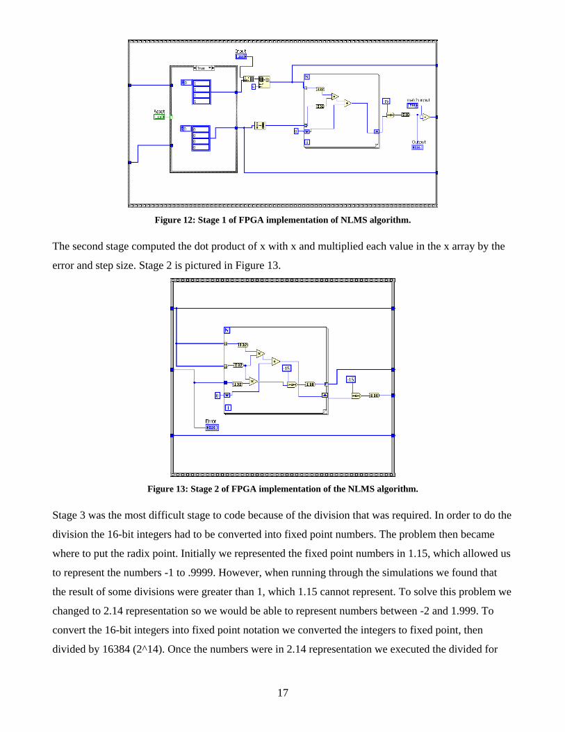
17

Figure 12: Stage 1 of FPGA implementation of NLMS algorithm.

The second stage computed the dot product of x with x and multiplied each value in the x array by the

error and step size. Stage 2 is pictured in Figure 13.

Figure 13: Stage 2 of FPGA implementation of the NLMS algorithm.

Stage 3 was the most difficult stage to code because of the division that was required. In order to do the

division the 16-bit integers had to be converted into fixed point numbers. The problem then became

where to put the radix point. Initially we represented the fixed point numbers in 1.15, which allowed us

to represent the numbers -1 to .9999. However, when running through the simulations we found that

the result of some divisions were greater than 1, which 1.15 cannot represent. To solve this problem we

changed to 2.14 representation so we would be able to represent numbers between -2 and 1.999. To

convert the 16-bit integers into fixed point notation we converted the integers to fixed point, then

divided by 16384 (2^14). Once the numbers were in 2.14 representation we executed the divided for

18

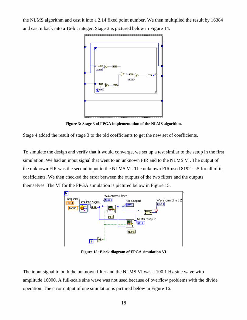
the NLMS algorithm and cast it into a 2.14 fixed point number. We then multiplied the result by 16384

and cast it back into a 16-bit integer. Stage 3 is pictured below in Figure 14.

Figure 3: Stage 3 of FPGA implementation of the NLMS algorithm.

Stage 4 added the result of stage 3 to the old coefficients to get the new set of coefficients.

To simulate the design and verify that it would converge, we set up a test similar to the setup in the first

simulation. We had an input signal that went to an unknown FIR and to the NLMS VI. The output of

the unknown FIR was the second input to the NLMS VI. The unknown FIR used 8192 = .5 for all of its

coefficients. We then checked the error between the outputs of the two filters and the outputs

themselves. The VI for the FPGA simulation is pictured below in Figure 15.

Figure 15: Block diagram of FPGA simulation VI

The input signal to both the unknown filter and the NLMS VI was a 100.1 Hz sine wave with

amplitude 16000. A full-scale sine wave was not used because of overflow problems with the divide

operation. The error output of one simulation is pictured below in Figure 16.

19

Figure 16: Error between the matching filter and the unknown filter as a function of time for FPGA simulation.

This simulation shows the algorithm converges and does work using only integers and fixed point

numbers. We then implemented the exact same NLMS, FIR and test VIs in LabVIEW 2009 for an

FPGA and simulated them.

After simulation, we compiled our FPGA VI, loaded it onto the sbRIO-9631, and created another VI

that ran on the processor for debugging purposes. The front panel of the VI that ran on the processor

had three graphs; one for each microphone and one for the output of the NLMS algorithm. For the

outside microphone we used a dbx RTA-M microphone connected to an ART USB Dual Pre

preamplifier. The inside microphone needed to be able to fit inside of an ear, so we used an EA-1843

electret microphone. In order to get the output of the microphones into the sbRIO we had to modify the

signals coming out of the microphones. The dbx RTA-M was connected to a preamplifier, which easily

allowed us to control the gain on the output of the microphone, but the EA-1843 was not connected to a

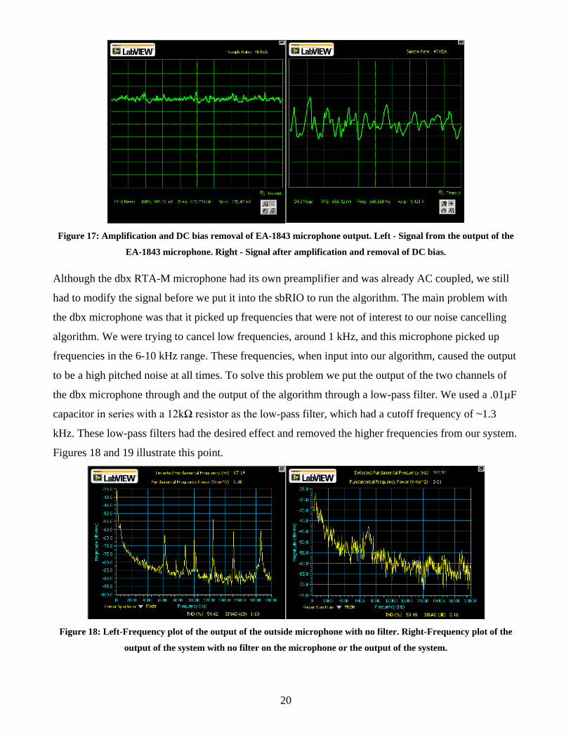
preamp. We had to amplify the signal coming out of the EA-1843 microphone and also remove a DC

offset that the microphone had. To amplify the signal we used a Texas Instruments LF347N op-amp

with a gain of around 90x. To remove the DC offset we put the output signal of the amplifier through

an AC coupling circuit. We used a 2.2µF capacitor and a 7.5 kΩ resistor in series with a 470Ω resistor

to accomplish this. Because of its large capacitance, this circuit also did not attenuate any signals of

interest. Figure 17 illustrates the effect the amplification and AC coupling had on the signal from the

EA-1843 microphone.

20

Figure 17: Amplification and DC bias removal of EA-1843 microphone output. Left - Signal from the output of the

EA-1843 microphone. Right - Signal after amplification and removal of DC bias.

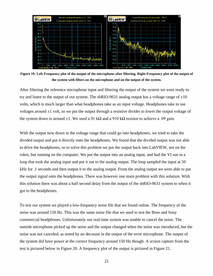
Although the dbx RTA-M microphone had its own preamplifier and was already AC coupled, we still

had to modify the signal before we put it into the sbRIO to run the algorithm. The main problem with

the dbx microphone was that it picked up frequencies that were not of interest to our noise cancelling

algorithm. We were trying to cancel low frequencies, around 1 kHz, and this microphone picked up

frequencies in the 6-10 kHz range. These frequencies, when input into our algorithm, caused the output

to be a high pitched noise at all times. To solve this problem we put the output of the two channels of

the dbx microphone through and the output of the algorithm through a low-pass filter. We used a .01µF

capacitor in series with a 12kΩ resistor as the low-pass filter, which had a cutoff frequency of ~1.3

kHz. These low-pass filters had the desired effect and removed the higher frequencies from our system.

Figures 18 and 19 illustrate this point.

Figure 18: Left-Frequency plot of the output of the outside microphone with no filter. Right-Frequency plot of the

output of the system with no filter on the microphone or the output of the system.

21

Figure 19: Left-Frequency plot of the output of the microphone after filtering. Right-Frequency plot of the output of

the system with filters on the microphone and on the output of the system.

After filtering the reference microphone input and filtering the output of the system we were ready to

try and listen to the output of our system. The sbRIO-9631 analog output has a voltage range of ±10

volts, which is much larger than what headphones take as an input voltage. Headphones take in use

voltages around ±1 volt, so we put the output through a resistive divider to lower the output voltage of

the system down to around ±1. We used a 91 kΩ and a 910 kΩ resistor to achieve a .09 gain.

With the output now down in the voltage range that could go into headphones, we tried to take the

divided output and put it directly onto the headphones. We found that the divided output was not able

to drive the headphones, so to solve this problem we put the output back into LabVIEW, not on the

robot, but running on the computer. We put the output into an analog input, and had the VI run in a

loop that took the analog input and put it out to the analog output. The loop sampled the input at 50

kHz for .1 seconds and then output it to the analog output. From the analog output we were able to put

the output signal onto the headphones. There was however one main problem with this solution. With

this solution there was about a half second delay from the output of the sbRIO-9631 system to when it

got to the headphones.

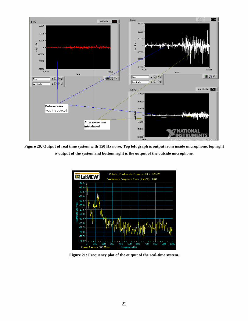
To test our system we played a low-frequency noise file that we found online. The frequency of the

noise was around 150 Hz. This was the same noise file that we used to test the Bose and Sony

commercial headphones. Unfortunately our real-time system was unable to cancel the noise. The

outside microphone picked up the noise and the output changed when the noise was introduced, but the

noise was not canceled, as noted by no decrease in the output of the error microphone. The output of

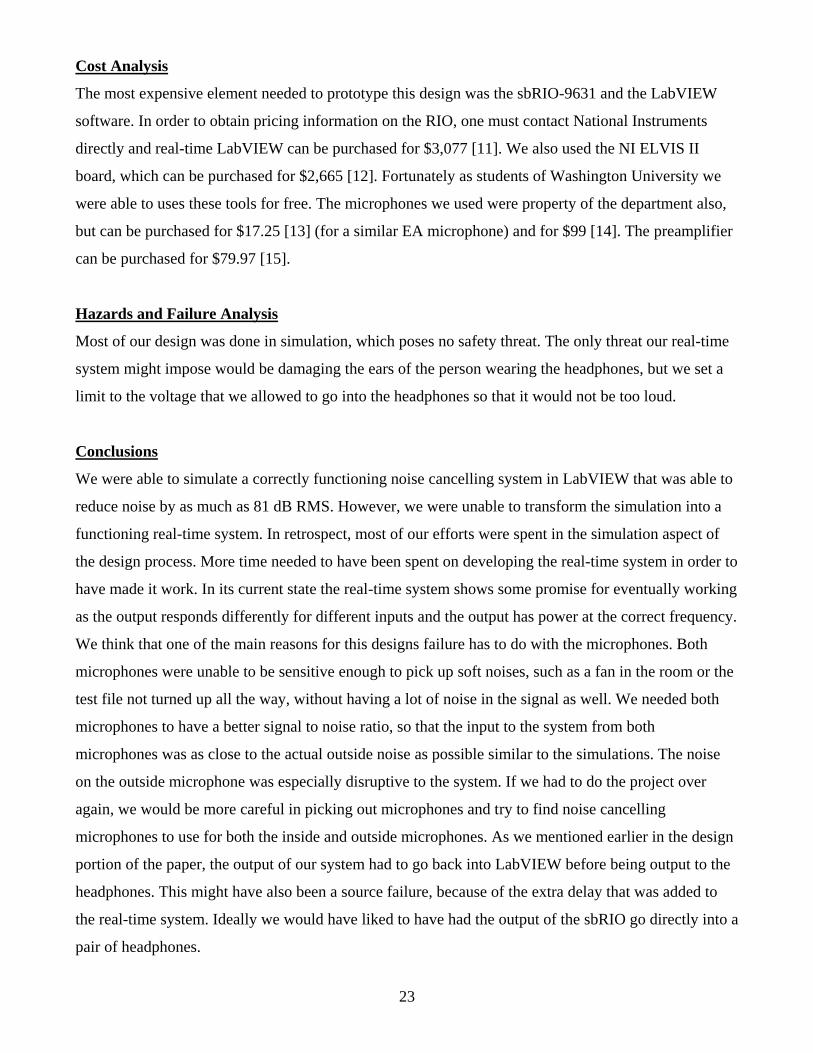
the system did have power at the correct frequency around 150 Hz though. A screen capture from the

test is pictured below in Figure 20. A frequency plot of the output is pictured in Figure 21.

22

Figure 20: Output of real time system with 150 Hz noise. Top left graph is output from inside microphone, top right

is output of the system and bottom right is the output of the outside microphone.

Figure 21: Frequency plot of the output of the real-time system.

23

Cost Analysis

The most expensive element needed to prototype this design was the sbRIO-9631 and the LabVIEW

software. In order to obtain pricing information on the RIO, one must contact National Instruments

directly and real-time LabVIEW can be purchased for $3,077 [11]. We also used the NI ELVIS II

board, which can be purchased for $2,665 [12]. Fortunately as students of Washington University we

were able to uses these tools for free. The microphones we used were property of the department also,

but can be purchased for $17.25 [13] (for a similar EA microphone) and for $99 [14]. The preamplifier

can be purchased for $79.97 [15].

Hazards and Failure Analysis

Most of our design was done in simulation, which poses no safety threat. The only threat our real-time

system might impose would be damaging the ears of the person wearing the headphones, but we set a

limit to the voltage that we allowed to go into the headphones so that it would not be too loud.

Conclusions

We were able to simulate a correctly functioning noise cancelling system in LabVIEW that was able to

reduce noise by as much as 81 dB RMS. However, we were unable to transform the simulation into a

functioning real-time system. In retrospect, most of our efforts were spent in the simulation aspect of

the design process. More time needed to have been spent on developing the real-time system in order to

have made it work. In its current state the real-time system shows some promise for eventually working

as the output responds differently for different inputs and the output has power at the correct frequency.

We think that one of the main reasons for this designs failure has to do with the microphones. Both

microphones were unable to be sensitive enough to pick up soft noises, such as a fan in the room or the

test file not turned up all the way, without having a lot of noise in the signal as well. We needed both

microphones to have a better signal to noise ratio, so that the input to the system from both

microphones was as close to the actual outside noise as possible similar to the simulations. The noise

on the outside microphone was especially disruptive to the system. If we had to do the project over

again, we would be more careful in picking out microphones and try to find noise cancelling

microphones to use for both the inside and outside microphones. As we mentioned earlier in the design

portion of the paper, the output of our system had to go back into LabVIEW before being output to the

headphones. This might have also been a source failure, because of the extra delay that was added to

the real-time system. Ideally we would have liked to have had the output of the sbRIO go directly into a

pair of headphones.

24

References

[1] A. Milosevic and U. Schaufelberger. (2005 December). Active Noise Control. Rapperswil,

Switzerland. [Online]. Available:

http://www.medialab.ch/archiv/pdf_studien_diplomarbeiten/da05/da2005-104_ActiveNoiseControl.pdf

[2] B. Brogdon, T. Deitch, K. Barnhart, and B. Antley, (2008, January), “Least mean squares adaptive

filters,” Connexions, Available: http://cnx.org/content/m15675/1.2/

[3] B. Siravana, N. Magotra, and P. Loizou, “A novel approach for single microphone active noise

cancellation,” presented at 45th

IEEE MWSCAS Conf., Tulsa, Oklahoma, Aug. 4-7, 2002.

[4] G. S. Kang and L. J. Fransen, “Experimentation with an adaptive noise-cancellation filter,” IEEE

Trans. on Circuits and Systems, vol. CAS-34, pp. 753-758, Jul. 1987.

[5] K. C. Zangi. (1993) A New Two-Sensor Active Noise Cancellation Algorithm. Cambridge, MA.

[Online]. Available: http://www.rle.mit.edu/dspg/documents/Two-sensoractive.pdf.

[6] Milosevic and U. Schaufelberger, “Active noise control,” Diploma thesis, University of Applied

Sciences Rapperswil, Rapperswil, Switzerland, 2005.

[7] Noise Cancelling Headphones. Sony Electronics Inc. Tokyo, Japan. [Online]. Available:

http://www.sonystyle.com/webapp/wcs/stores/servlet/ProductDisplay?catalogId=10551&storeId=1015

1&langId=-1&productId=8198552921665368379

[8] QuietComfort® 15 Acoustic Noise Cancelling® headphones. Bose Corporation. The Mountain,

Framingham, MA. [Online]. Available:

http://www.bose.com/controller?url=/shop_online/headphones/noise_cancelling_headphones/quietcom

fort_15/index.jsp

[9] Wikipedia Contributors. (2010, April). Least mean squares filter. [Online]. Available:

http://en.wikipedia.org/wiki/Least_mean_squares_filter

[10] Z. Feng, X. Shi, and H. Huang, “An improved adaptive noise cancelling method,” Canadian

Conference on Electrical and Computer Engineering, 1993, pp. 47-50.

[11] National Instruments Corporation. Austin, TX. [Online]. Available:

http://ohm.ni.com/advisors/devsuite?rec=Realtime_FPGA

[12] National Instruments Corporation. Austin, TX. [Online]. Available:

http://sine.ni.com/nips/cds/view/p/lang/en/nid/13137

[13] Digi-Key Corporation. Thief River Falls, MN. [Online]. Available:

http://search.digikey.com/scripts/DkSearch/dksus.dll

[14] zZounds Music, LLC. Midland Park, NJ. [Online]. Available: http://www.zzounds.com/item--

DBXRTAM

25

[15] Sweetwater Sound Inc. Fort Wayne, IN. [Online]. Available:

http://www.sweetwater.com/store/detail/USBDualPrePS