Digit Recognizer - Research in Scientific Computing in ... would like to add them to my immediate...

Digit Recognizer

Using Machine Learning to

Decipher Handwritten Digits

MTH 499 CSUMS FALL 2012

Matheus M. Lelis

Undergraduate Student

Dept. of Mathematics

UMass Dartmouth

Dartmouth MA 02747

[email protected]

Abstract

The goal of this research project is to create an artificial neural network machine able to recognize

handwritten letters and numbers. Through multi-class classification and using the backpropagation

algorithm, the proposed machine should be able to learn the difference between each handwritten number

and after proper training, correctly guess the number in the inputted image. The machine will be written

in MATLAB® language using new original code and pre-existing code when applicable.

1

Matheus M. Lelis MTH 499 CSUMS (FALL 2012): Digit Recognizer

Contents1 Problem Formulation 3

1.1 Backgound . . . . . . . . . . . . . . . . . . . . . . . . . . . . . . . . . . . . . . . . . . . . . . . . 3

1.2 Application . . . . . . . . . . . . . . . . . . . . . . . . . . . . . . . . . . . . . . . . . . . . . . . . 3

1.3 Research Goals . . . . . . . . . . . . . . . . . . . . . . . . . . . . . . . . . . . . . . . . . . . . . . 3

2 Methodology 4

2.1 Artificial Neural Networks . . . . . . . . . . . . . . . . . . . . . . . . . . . . . . . . . . . . . . . . 4

2.1.1 Feed Forward . . . . . . . . . . . . . . . . . . . . . . . . . . . . . . . . . . . . . . . . . . . . . . 4

2.1.2 Cost Function . . . . . . . . . . . . . . . . . . . . . . . . . . . . . . . . . . . . . . . . . . . . . 4

2.2 Backpropagation . . . . . . . . . . . . . . . . . . . . . . . . . . . . . . . . . . . . . . . . . . . . . 5

3 Results: The Machine 6

3.1 Data Files . . . . . . . . . . . . . . . . . . . . . . . . . . . . . . . . . . . . . . . . . . . . . . . . . 6

3.1.1 mydata.mat . . . . . . . . . . . . . . . . . . . . . . . . . . . . . . . . . . . . . . . . . . . . . . . 6

3.1.2 weights.mat . . . . . . . . . . . . . . . . . . . . . . . . . . . . . . . . . . . . . . . . . . . . . . . 6

3.2 Function Files . . . . . . . . . . . . . . . . . . . . . . . . . . . . . . . . . . . . . . . . . . . . . . . 6

3.2.1 costfun.m . . . . . . . . . . . . . . . . . . . . . . . . . . . . . . . . . . . . . . . . . . . . . . . . 6

3.2.2 fmincg.m . . . . . . . . . . . . . . . . . . . . . . . . . . . . . . . . . . . . . . . . . . . . . . . . 6

3.2.3 predict.m . . . . . . . . . . . . . . . . . . . . . . . . . . . . . . . . . . . . . . . . . . . . . . . . 6

3.2.4 shownumber.m . . . . . . . . . . . . . . . . . . . . . . . . . . . . . . . . . . . . . . . . . . . . . 6

3.3 Main Files . . . . . . . . . . . . . . . . . . . . . . . . . . . . . . . . . . . . . . . . . . . . . . . . . 6

3.3.1 learning.m . . . . . . . . . . . . . . . . . . . . . . . . . . . . . . . . . . . . . . . . . . . . . . . 6

3.3.2 guessing.m . . . . . . . . . . . . . . . . . . . . . . . . . . . . . . . . . . . . . . . . . . . . . . . 7

4 Conclusion 7

4.1 Semester in Review . . . . . . . . . . . . . . . . . . . . . . . . . . . . . . . . . . . . . . . . . . . . 7

4.2 Future Goals . . . . . . . . . . . . . . . . . . . . . . . . . . . . . . . . . . . . . . . . . . . . . . . 7

5 Acknowledgements 7

6 Apendix 8

6.1 costfun.m . . . . . . . . . . . . . . . . . . . . . . . . . . . . . . . . . . . . . . . . . . . . . . . . . 8

6.2 fmincg.m . . . . . . . . . . . . . . . . . . . . . . . . . . . . . . . . . . . . . . . . . . . . . . . . . 9

6.3 guessing.m . . . . . . . . . . . . . . . . . . . . . . . . . . . . . . . . . . . . . . . . . . . . . . . . 12

6.4 learning.m . . . . . . . . . . . . . . . . . . . . . . . . . . . . . . . . . . . . . . . . . . . . . . . . . 13

6.5 predict.m . . . . . . . . . . . . . . . . . . . . . . . . . . . . . . . . . . . . . . . . . . . . . . . . . 14

6.6 shownumber.m . . . . . . . . . . . . . . . . . . . . . . . . . . . . . . . . . . . . . . . . . . . . . . 14

7 References 15

of 15


Problem Formulation

1.1 Backgound

I had originally found his problem online, where it had been posted on the Kaggletm website as a tutorial

competition designed to introduce people to Machine Learning. As I have great interest in the subject I

decided to attempt to solve it and when I accomplished it, then I would move to working in a more advanced

version of the problem. Before I could do anything advanced I would have to learn the basics, and digit

recognition, being a classic example in the teaching of Machine Learning was a great place to start.

1.2 Application

There is nothing wrong in researching for the sake of research, but for this semester I wanted to work with

something that could have real world applications. Digit recognizers are already being used in the real world

for different things such as the digitization of written personal checks by banking institutions and recognizing

zip codes on envelopes. I would personally like to be able to get my research to the point where it can be

applied to solving CAPTCHAs(Figure 1), which are a security measure on websites. Some have questioned

whether this a good direction for this type of software, but only through testing of our current security

measures can we assure that they remain updated and keep our data safe

Figure(1): An example of a modern CAPTCHA,

courtesy of Wikimedia Commons

1.3 Research Goals

Coming in at the begining of the semester without a real grasp of the task I had at hand, I set a rather

hopeful set of goals for myself. The goals set were:

• Increase my working knowledge of Machine Learning

• Use that to create a machine able to take an image of a handwritten single digit and correctly guess

what that digit is.

• Expand working machine to work with all alphanumeric characters.

• Manipulate working machine to be able to accept a CAPTCHA image input and solve it.

of 15


Methodology

2.1 Artificial Neural Networks

An artificial neural network is a mathematical model inspired by the neural networks found in the human

brain. A neural network consists of interconnected nodes with varying amounts of layers. The most basic

artificial neural network will have three layers, the input layer, a hidden layer, and the final output layer.

This structure can be seen in Figure 2 below.

Figure(2): The visual representation of a neural network

2.1.1 Feed Forward

As shown in Figure 2, a feed forward neural network only goes in one direction as represented by the arrows.

This type of neural network is one the most simple types of neural networks and differs from more advanced

networks as it does not have any loops inside it’s hidden layers. The input comes in sorting through the

hidden layers as necessary, but never goes back a layer.

2.1.2 Cost Function

The cost function which allows the artificial neural network to make decisions is a more detailed logistic

regression fuction. The cost funtion is shown bellow:

J(θ) =1

m

m∑i=m

K∑k=1

[−y(i)k log

((hθ(xi))k

)−(

1 − y(i)k

)log(

1 −(hθ

(x(i)))

k

)],

where hθ(x(i))

is computed as shown above in Figure 2 and K is the amount of classes or outputs we have.

In the case of our Machine this will be 10 since we have all digits from 0-9. The versatility of this function

would allow for further expansion into characters, or more classes in the future.

of 15


2.2 Backpropagation

While we can use the cost function to fill out the neural network, we need an extra algorithm to optimize

the cost function and allow the machine to learn. The backpropagation algorithm that allows this to work

can be seen as follow

• Given a training example(x(t), y(t)

), first forward propagate to compute all the activations throughout

the network, including the hθ(x) hypothesis which makes up the output node.

• For each node j in layer l, calculate the error by solving for δ(l)j in the manner shown in Figure 3. We

can see that we start in the output nodes and work backwards, giving the algorithm its name.

• Once all of that is done, we update the weights in the algorithm and repeat all the steps as many

iterations as needed.

Figure(2): A neural network showing how the

backpropagation algorithm works in it

of 15


Results: The Machine

The final machine is made up of two main files, two data files, and four functions. The description for each

is outlined bellow, and the code for the functions and main files can be found in the appendix.

3.1 Data Files

3.1.1 mydata.mat

The sample data given by the Kaggle website consisted of a large .csv file which contained the data for

several thousand 28px by 28px images of handwritten numbers. The first step towards building this machine

was to extract this data using MATLAB® and convert it into a .mat file consisting of two matrices, one

which would have the data and another which would have the answers.

3.1.2 weights.mat

With data but with no weights, I would then create a file, which would have the weight matrices, but they

would all be filled with zeros. After running the Learning code once the zeros would be replaced with real

parameters, the more iterations I ran, the more accurate the weights would become.

3.2 Function Files

3.2.1 costfun.m

This function is where most of the math exists. It’s in charge of taking all of the mathematical formulas and

the back propagation algorithm and turning it into code. Together with fmincg.m they make up the muscle

that make this machine work. This will create the cost function for a 3 layer neural network whenever it is

called upon.

3.2.2 fmincg.m

This function was created by Carl Edward Rasmussen and is used to minimize a continuous differentiable

multivariate function, which is precisely what we need to do to make the backpropagation algorithm work.

By running the weights through this function we can update them and lower the error.

3.2.3 predict.m

An overloading of a pre-defined method, this function allows the predict method work with the Theta and

X values I’ll be feeding it so that it can predict what the number in the image is.

3.2.4 shownumber.m

This function allows me to visualize the data given by Kaggle. It can handle both a random selection of

data or a single value, which becomes useful when testing to see if it works or not.

3.3 Main Files

3.3.1 learning.m

The learning.m file when run will open the file with all the data, then with the weights. It will proceed

to create a cost function using the functions provided and then begin to learn by minimizing the function

using the fmincg.m function. Depending on the amount of iterations it is set to perform, it can run for a

of 15


few minutes to hours. After it is done running it will save the new parameters back into the weights.mat

file. It also tests the current sets accuracy. After thousands of iterations, I have managed to achieve almost

91% accuracy.

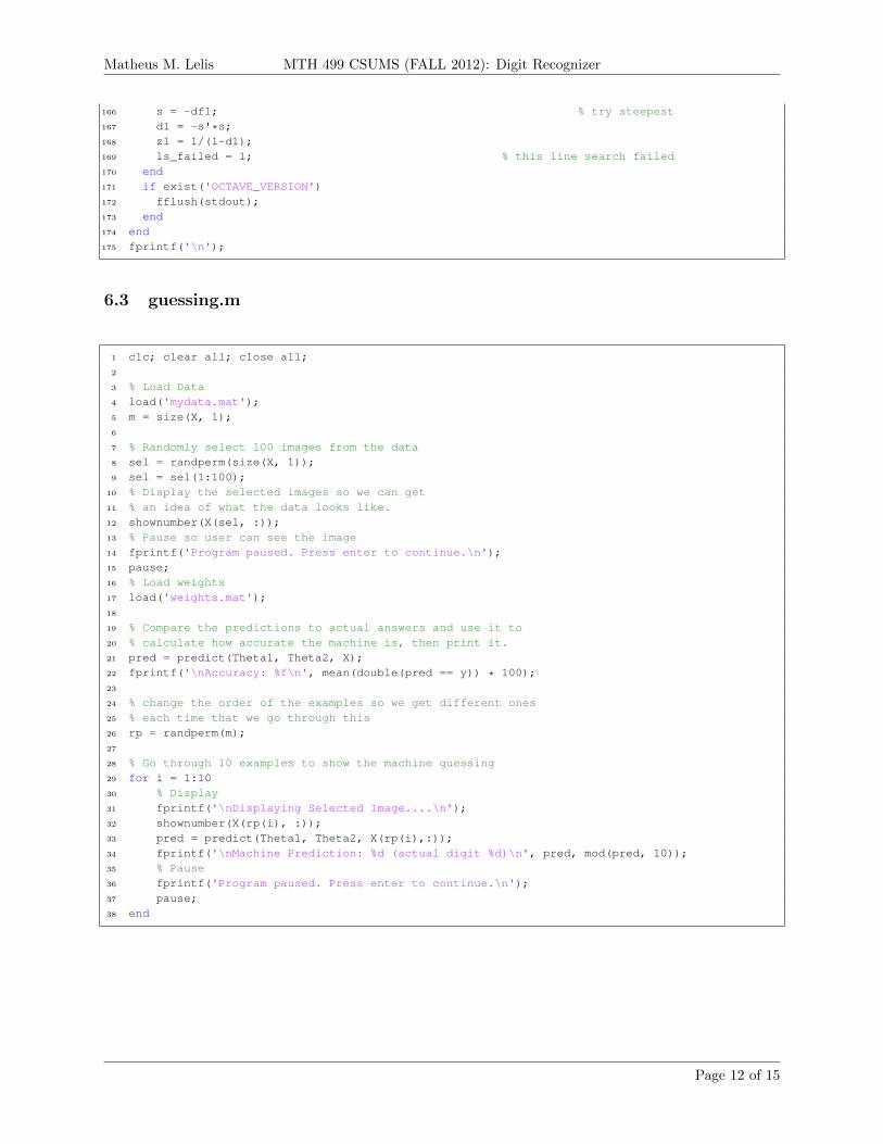
3.3.2 guessing.m

This program allows us to visualize the machine functioning. It will first print out a random selection of

data just so the user can see what the machine is working with. It will then proceed to perform 10 test

runs of guessing what an image is. It will display the image and print its guess. After then tenth guess the

program exits.

Conclusion

4.1 Semester in Review

I began the semester with some very hopeful goals and soon realized how much work it was really going to

be. Given my course load and working part time I didn’t end up having as much time to learn about the

subject as I hoped to. Time aside I was able to meet half of my goals this semester and lay a solid foundation

for any future research I may want to do in this particular area. One of the biggest challenges I ended up

facing this semester was actually finding data to work with when it came to dealing with the alphanumeric

characters. I’m fairly certain that the machine is versatile enough to be able to accept more classes with a

few tweaks, but being unable to find letters left me without anything to work with. Creating the data was

an option, but time didn’t allow me to do that. I hope for the future to dedicate some more time for this

research and e able to meet at least all of my initial goals.

4.2 Future Goals

Sometimes in research time runs out and decisions have to be made regarding the direction of the research

for that period. As a result some of the things I wanted to work on for this semester didn’t happen, and so

I would like to add them to my immediate list of future goals.

• Expand the machine so as to work with not just digits but all alphanumeric characters. Use this

machine to attempt to solve CAPTCHAS.

• To examine alternative Machine Learning algorithms while working on the possibility of creating a new

algorithm that might work better for this particular task.

• Possibly parallelizing my code, to speed up the learning process when starting with zero weights.

There might be more things to add to this project, but I believe that focusing on these two first will open up

a whole new batch of questions and problems to be solved, creating a lasting and worthwhile research topic.

Acknowledgements

I would like to offer a special thanks to my advisor, Dr. Alfa Heryudono, for his help and guidance as I

worked on this project this past semester. Also, I want to thank the math department of the University of

Massachusetts Dartmouth, especially to the faculty engaged in the CSUMS program. Lastly I would like to

thank the National Science Foundation for providing the funding for the CSUMS program and for making

this last semester of work possible.

of 15


Appendix

6.1 costfun.m

1 function [J grad] = costfun(params, input, hidden, labels, X, y, lambda)2 % First thing we do is take out Theta1 and Theta2 from params3 Theta1 = reshape(params(1:hidden * (input + 1)), hidden, (input + 1));4 Theta2 = reshape(params((1 + (hidden * (input + 1))):end), labels, (hidden + 1));5

6 % Next we have to setup the variables7 m = size(X, 1);8

9 % Then we declare the values we're going to return.10 J = 0;11 gTheta1 = zeros(size(Theta1));12 gTheta2 = zeros(size(Theta2));13

14 X = [ones(m,1) X];15

16 % First we need to do the forward propagation so that a1 = X;17 a2 = 1.0 ./ (1.0 + exp(-Theta1 * X'));18 a2 = [ones(m,1) a2'];19

20 % hTheta equals z321 hTheta = 1.0 ./ (1.0 + exp(-Theta2 * a2'));22

23 % Now change the labels so they become vectors of only 0s or 1s24 yk = zeros(labels, m);25 for i=1:m,26 yk(y(i),i)=1;27 end28 % Declare the cost function29 J = (1/m) * sum ( sum ( (-yk) .* log(hTheta) - (1-yk) .* log(1-hTheta) ));30

31 % Get the first terms of each matrix32 t1 = Theta1(:,2:size(Theta1,2));33 t2 = Theta2(:,2:size(Theta2,2));34

35 % Declae the formula for regularization36 Reg = lambda * (sum( sum ( t1.ˆ 2 )) + sum( sum ( t2.ˆ 2 ))) / (2*m);37

38 % Create the cost function with regularization39 J = J + Reg;40

41 % Begin the Backpropagation42 for t=1:m,43 a1 = X(t,:); % X already has bias44 z2 = Theta1 * a1';45 % Activation for a246 a2 = 1.0 ./ (1.0 + exp(-z2));47 a2 = [1 ; a2]; % add in the bias48 z3 = Theta2 * a2;49 % Activation for a350 a3 = 1.0 ./ (1.0 + exp(-z3));51 z2 = [1; z2]; % add in the bias52 % Get the columns of t element53 ∆3 = a3 - yk(:,t);54 ∆2 = (Theta2' * ∆3) .* (1.0 ./ (1.0 + exp(-z2))) .* (1 - (1.0 ./ (1.0 + exp(-z2))));55 ∆2 = ∆2(2:end);

of 15


56 % get the gradients57 gTheta2 = gTheta2 + ∆3 * a2';58 gTheta1 = gTheta1 + ∆2 * a1;59 end;60

61 % Regularize the function62 gTheta1(:, 1) = gTheta1(:, 1) ./ m;63 gTheta1(:, 2:end) = gTheta1(:, 2:end) ./ m + ((lambda/m) * Theta1(:, 2:end));64 gTheta2(:, 1) = gTheta2(:, 1) ./ m;65 gTheta2(:, 2:end) = gTheta2(:, 2:end) ./ m + ((lambda/m) * Theta2(:, 2:end));66

67 % Open up the gradients68 grad = [gTheta1(:) ; gTheta2(:)];69

70 end

6.2 fmincg.m

1 function [X, fX, i] = fmincg(f, X, options, P1, P2, P3, P4, P5)2 % Minimize a continuous differentialble multivariate function. Starting point3 % is given by "X" (D by 1), and the function named in the string "f", must4 % return a function value and a vector of partial derivatives. The Polack-5 % Ribiere flavour of conjugate gradients is used to compute search directions,6 % and a line search using quadratic and cubic polynomial approximations and the7 % Wolfe-Powell stopping criteria is used together with the slope ratio method8 % for guessing initial step sizes. Additionally a bunch of checks are made to9 % make sure that exploration is taking place and that extrapolation will not

10 % be unboundedly large. The "length" gives the length of the run: if it is11 % positive, it gives the maximum number of line searches, if negative its12 % absolute gives the maximum allowed number of function evaluations. You can13 % (optionally) give "length" a second component, which will indicate the14 % reduction in function value to be expected in the first line-search (defaults15 % to 1.0). The function returns when either its length is up, or if no further16 % progress can be made (ie, we are at a minimum, or so close that due to17 % numerical problems, we cannot get any closer). If the function terminates18 % within a few iterations, it could be an indication that the function value19 % and derivatives are not consistent (ie, there may be a bug in the20 % implementation of your "f" function). The function returns the found21 % solution "X", a vector of function values "fX" indicating the progress made22 % and "i" the number of iterations (line searches or function evaluations,23 % depending on the sign of "length") used.24 %25 % Usage: [X, fX, i] = fmincg(f, X, options, P1, P2, P3, P4, P5)26 %27 % See also: checkgrad28 %29 % Copyright (C) 2001 and 2002 by Carl Edward Rasmussen. Date 2002-02-1330 %31 %32 % (C) Copyright 1999, 2000 & 2001, Carl Edward Rasmussen33 %34 % Permission is granted for anyone to copy, use, or modify these35 % programs and accompanying documents for purposes of research or36 % education, provided this copyright notice is retained, and note is37 % made of any changes that have been made.38 %39 % These programs and documents are distributed without any warranty,40 % express or implied. As the programs were written for research41 % purposes only, they have not been tested to the degree that would be

of 15


42 % advisable in any important application. All use of these programs is43 % entirely at the user's own risk.44 %45 % [ml-class] Changes Made:46 % 1) Function name and argument specifications47 % 2) Output display48 %49

50 % Read options51 if exist('options', 'var') && ¬isempty(options) && isfield(options, 'MaxIter')52 length = options.MaxIter;53 else54 length = 100;55 end56

57

58 RHO = 0.01; % a bunch of constants for line searches59 SIG = 0.5; % RHO and SIG are the constants in the Wolfe-Powell conditions60 INT = 0.1; % don't reevaluate within 0.1 of the limit of the current bracket61 EXT = 3.0; % extrapolate maximum 3 times the current bracket62 MAX = 20; % max 20 function evaluations per line search63 RATIO = 100; % maximum allowed slope ratio64

65 argstr = ['feval(f, X']; % compose string used to call function66 for i = 1:(nargin - 3)67 argstr = [argstr, ',P', int2str(i)];68 end69 argstr = [argstr, ')'];70

71 if max(size(length)) == 2, red=length(2); length=length(1); else red=1; end72 S=['Iteration '];73

74 i = 0; % zero the run length counter75 ls_failed = 0; % no previous line search has failed76 fX = [];77 [f1 df1] = eval(argstr); % get function value and gradient78 i = i + (length<0); % count epochs?!79 s = -df1; % search direction is steepest80 d1 = -s'*s; % this is the slope81 z1 = red/(1-d1); % initial step is red/(|s|+1)82

83 while i < abs(length) % while not finished84 i = i + (length>0); % count iterations?!85

86 X0 = X; f0 = f1; df0 = df1; % make a copy of current values87 X = X + z1*s; % begin line search88 [f2 df2] = eval(argstr);89 i = i + (length<0); % count epochs?!90 d2 = df2'*s;91 f3 = f1; d3 = d1; z3 = -z1; % initialize point 3 equal to point 192 if length>0, M = MAX; else M = min(MAX, -length-i); end93 success = 0; limit = -1; % initialize quanteties94 while 195 while ((f2 > f1+z1*RHO*d1) | (d2 > -SIG*d1)) & (M > 0)96 limit = z1; % tighten the bracket97 if f2 > f198 z2 = z3 - (0.5*d3*z3*z3)/(d3*z3+f2-f3); % quadratic fit99 else

100 A = 6*(f2-f3)/z3+3*(d2+d3); % cubic fit101 B = 3*(f3-f2)-z3*(d3+2*d2);102 z2 = (sqrt(B*B-A*d2*z3*z3)-B)/A; % numerical error possible - ok!103 end

of 15


104 if isnan(z2) | isinf(z2)105 z2 = z3/2; % if we had a numerical problem then bisect106 end107 z2 = max(min(z2, INT*z3),(1-INT)*z3); % don't accept too close to limits108 z1 = z1 + z2; % update the step109 X = X + z2*s;110 [f2 df2] = eval(argstr);111 M = M - 1; i = i + (length<0); % count epochs?!112 d2 = df2'*s;113 z3 = z3-z2; % z3 is now relative to the location of z2114 end115 if f2 > f1+z1*RHO*d1 | d2 > -SIG*d1116 break; % this is a failure117 elseif d2 > SIG*d1118 success = 1; break; % success119 elseif M == 0120 break; % failure121 end122 A = 6*(f2-f3)/z3+3*(d2+d3); % make cubic extrapolation123 B = 3*(f3-f2)-z3*(d3+2*d2);124 z2 = -d2*z3*z3/(B+sqrt(B*B-A*d2*z3*z3)); % num. error possible - ok!125 if ¬isreal(z2) | isnan(z2) | isinf(z2) | z2 < 0 % num prob or wrong sign?126 if limit < -0.5 % if we have no upper limit127 z2 = z1 * (EXT-1); % the extrapolate the maximum amount128 else129 z2 = (limit-z1)/2; % otherwise bisect130 end131 elseif (limit > -0.5) & (z2+z1 > limit) % extraplation beyond max?132 z2 = (limit-z1)/2; % bisect133 elseif (limit < -0.5) & (z2+z1 > z1*EXT) % extrapolation beyond limit134 z2 = z1*(EXT-1.0); % set to extrapolation limit135 elseif z2 < -z3*INT136 z2 = -z3*INT;137 elseif (limit > -0.5) & (z2 < (limit-z1)*(1.0-INT)) % too close to limit?138 z2 = (limit-z1)*(1.0-INT);139 end140 f3 = f2; d3 = d2; z3 = -z2; % set point 3 equal to point 2141 z1 = z1 + z2; X = X + z2*s; % update current estimates142 [f2 df2] = eval(argstr);143 M = M - 1; i = i + (length<0); % count epochs?!144 d2 = df2'*s;145 end % end of line search146

147 if success % if line search succeeded148 f1 = f2; fX = [fX' f1]';149 fprintf('%s %4i | Cost: %4.6e\r', S, i, f1);150 s = (df2'*df2-df1'*df2)/(df1'*df1)*s - df2; % Polack-Ribiere direction151 tmp = df1; df1 = df2; df2 = tmp; % swap derivatives152 d2 = df1'*s;153 if d2 > 0 % new slope must be negative154 s = -df1; % otherwise use steepest direction155 d2 = -s'*s;156 end157 z1 = z1 * min(RATIO, d1/(d2-realmin)); % slope ratio but max RATIO158 d1 = d2;159 ls_failed = 0; % this line search did not fail160 else161 X = X0; f1 = f0; df1 = df0; % restore point from before failed line search162 if ls_failed | i > abs(length) % line search failed twice in a row163 break; % or we ran out of time, so we give up164 end165 tmp = df1; df1 = df2; df2 = tmp; % swap derivatives

of 15


166 s = -df1; % try steepest167 d1 = -s'*s;168 z1 = 1/(1-d1);169 ls_failed = 1; % this line search failed170 end171 if exist('OCTAVE_VERSION')172 fflush(stdout);173 end174 end175 fprintf('\n');

6.3 guessing.m

1 clc; clear all; close all;2

3 % Load Data4 load('mydata.mat');5 m = size(X, 1);6

7 % Randomly select 100 images from the data8 sel = randperm(size(X, 1));9 sel = sel(1:100);

10 % Display the selected images so we can get11 % an idea of what the data looks like.12 shownumber(X(sel, :));13 % Pause so user can see the image14 fprintf('Program paused. Press enter to continue.\n');15 pause;16 % Load weights17 load('weights.mat');18

19 % Compare the predictions to actual answers and use it to20 % calculate how accurate the machine is, then print it.21 pred = predict(Theta1, Theta2, X);22 fprintf('\nAccuracy: %f\n', mean(double(pred == y)) * 100);23

24 % change the order of the examples so we get different ones25 % each time that we go through this26 rp = randperm(m);27

28 % Go through 10 examples to show the machine guessing29 for i = 1:1030 % Display31 fprintf('\nDisplaying Selected Image....\n');32 shownumber(X(rp(i), :));33 pred = predict(Theta1, Theta2, X(rp(i),:));34 fprintf('\nMachine Prediction: %d (actual digit %d)\n', pred, mod(pred, 10));35 % Pause36 fprintf('Program paused. Press enter to continue.\n');37 pause;38 end

of 15


6.4 learning.m

1 clc; clear all; close all;2

3 % 28x28 Input Images of Digits create the input layer4 input = 784;5 % 25 hidden units in the middle layer6 hidden = 25;7 % 10 labels, from 1 to 10 where 10 is used for 08 labels = 10;9

10 % Load Data11 load('mydata.mat');12 m = size(X, 1);13

14 % Load the weights15 load('weights.mat');16

17 % Open parameters from weights18 initial_params = [Theta1(:) ; Theta2(:)];19

20 % Begin training the Neural Network using Back Propagation21 fprintf('\nTraining Neural Network... \n')22

23 % the more iterations, the more it learns but takes a lot more time.24 options = optimset('MaxIter', 10);25

26 lambda = 3; % part of the optimizing function27

28 % declare the cost function so we can minimize it29 costFunction = @(p) costfun(p, input, hidden, labels, X, y, lambda);30

31 % here we use fmincg to minimzie the cost, using tic toc to time it32 tic;33 [params, cost] = fmincg(costFunction, initial_params, options);34 toc;35

36 % Now we take out Theta1 and Theta2 from params37 Theta1 = reshape(params(1:hidden * (input + 1)), hidden, (input + 1));38 Theta2 = reshape(params((1+(hidden*(input+1))):end), labels, (hidden+1));39

40 % Here we have it predict all the results41 pred = predict(Theta1, Theta2, X);42

43 % We then compare the predictions to real answers and44 % with that we can calculate how accurate the machine is45 fprintf('\nAccuracy: %f\n', mean(double(pred == y)) * 100);46

47 % Finally we save the new weights back into the weights file48 save('weights.mat', 'Theta1', 'Theta2');

of 15


6.5 predict.m

1 function p = predict(Theta1, Theta2, X)2 m = size(X, 1);3 labels = size(Theta2, 1);4

5 % declare the variables that will be returned6 p = zeros(size(X, 1), 1);7

8 h1 = 1.0 ./ (1.0 + exp(-([ones(m, 1) X] * Theta1')));9 h2 = 1.0 ./ (1.0 + exp(-([ones(m, 1) h1] * Theta2')));

10 [dummy, p] = max(h2, [], 2);11

12 end

6.6 shownumber.m

1 function [h, imageShow] = shownumber(X)2 % Gray Image3 colormap(gray);4

5 % Figure out how many images came in6 amount = size(X, 1);7

8 % Make it so that it comes out as a square9 t = sqrt(amount);

10 t = t - mod(t, 1);11

12 imageShow = zeros(30*t,30*t);13

14 count = 1;15 level = 0;16 level2 = 0;17 for n=1:amount18 for i=(2+level2):(29+level2)19 for j=(2+level):(29+level)20 imageShow(i,j) = X(n,count) + 100;21 count = count+1;22 end23 end24 count = 1;25 level = level+30;26 if (mod(n,t) == 0)27 level2 = level2+30;28 level = 0;29 end30 end31 % Display Image32 h = imagesc(imageShow);33 % Hide the axis34 axis image off35

36 drawnow;37 end

of 15


References

Alex Holehouse. Neural networks - learning, 2011. URL http://www.holehouse.org/mlclass/09_

Neural_Networks_Learning.html.

Kaggle Inc. Description - digit recognizer, 2012. URL http://www.kaggle.com/c/

digit-recognizer.

Pete McCollum. An introduction to back-propagation neural networks, 1998. URL http://www.

seattlerobotics.org/encoder/nov98/neural.html.

Wikipedia. Artificial neural network — wikipedia, the free encyclopedia, 2012a. URL http://en.

wikipedia.org/w/index.php?title=Artificial_neural_network&oldid=528058378.

Wikipedia. Backpropagation — wikipedia, the free encyclopedia, 2012b. URL http://en.wikipedia.

org/w/index.php?title=Backpropagation&oldid=528691184.

Wikipedia. Feedforward neural network — wikipedia, the free encyclopedia, 2012c. URL http://en.

wikipedia.org/w/index.php?title=Feedforward_neural_network&oldid=523159510.

of 15

Digit Recognizer - Research in Scientific Computing in ... would like to add them to my immediate...

Documents

Transcript of Digit Recognizer - Research in Scientific Computing in ... would like to add them to my immediate...