Difﬁculties in computing the fundamental distortion mode in...

Difficulties in computing the fundamentaldistortion mode in Coriolis mass flow meters

CLAPDE 2008Simon Shaw

people.brunel.ac.uk/˜icsrsss

[email protected]

BICOM and Mathematical Sciences, Brunel University, England

Simon Shaw, CLAPDE (Durham) 2008 – p.1/34

Focus

The Coriolis effect

Coriolis mass flow meters

Collaboration and background

Eigenvalue problem & results


Coriolis

Gaspard-Gustave de Coriolis (Gustave

Coriolis, May 21, 1792 — September 19,

1843) published the paper that described

the effect that now bears his name in

1835: Sur les équations du mouvement

relatif des systèmes de corps (On the

equations of relative motion of a system

of bodies).

Source:en.wikipedia.org/wiki/Gaspard-Gustave_Coriolis


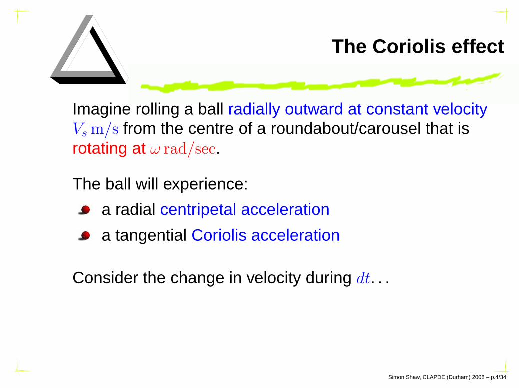
The Coriolis effect

Imagine rolling a ball radially outward at constant velocityVs m/s from the centre of a roundabout/carousel that isrotating at ω rad/sec.

The ball will experience:

a radial centripetal acceleration

a tangential Coriolis acceleration

Consider the change in velocity during dt. . .


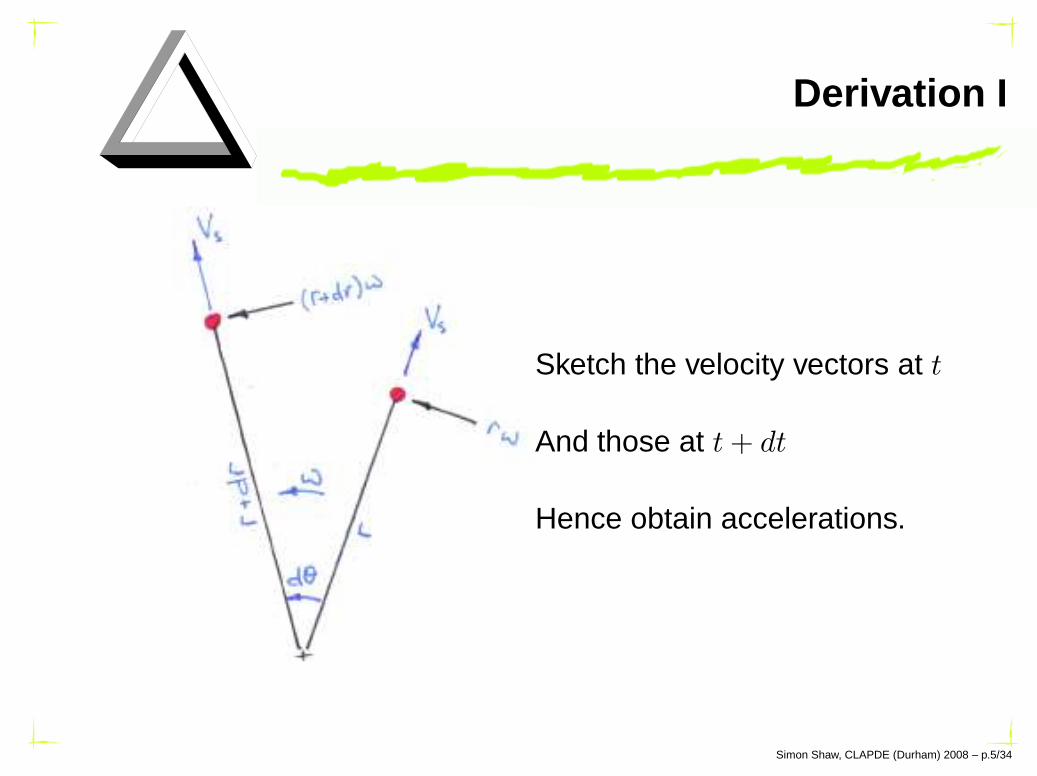
Derivation I

Sketch the velocity vectors at t

And those at t + dt

Hence obtain accelerations.


Derivation II

Change in tangential velocity

Vs dθ + ω dr

Change in radial velocity

rω dθ

Divide by dt to get acceleration:

tangential: 2ωVs Coriolis

radial: rω2 Centripetal


Pipe meter physics I

Metal pipe carries a plug flow of fluid at velocity V .

Pipe also vibrated by electromagnetic sine

Bending theory applies


Pipe meter physics II

Right end: fluid particle = ball on roundabout.

Coriolis acceleration implies force implies deformation.

Left end: Coriolis force is in opposite direction.Simon Shaw, CLAPDE (Durham) 2008 – p.8/34

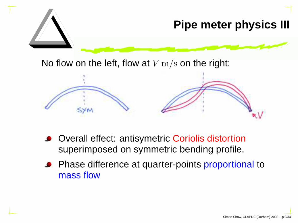
Pipe meter physics III

No flow on the left, flow at V m/s on the right:

Overall effect: antisymetric Coriolis distortionsuperimposed on symmetric bending profile.

Phase difference at quarter-points proportional tomass flow


So what?

Why does this matter?

Coriolis distortion is an inertial effect and isproportional to the mass (not volume) flow rate.

Mass flow is measured directly not by the indirectconversion of volume flow (e.g. bubbles).

Important for accuracy:Custodial transfersmedical drug dosing

Meters range from over 1 metre diameter tomicro-machined (fits on a thumb).


Example from wikipedia

An illustrative example:

No flow

With flow

Courtesy wikipedia.


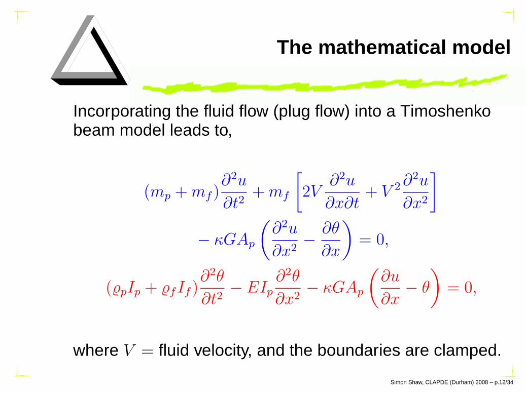
The mathematical model

Incorporating the fluid flow (plug flow) into a Timoshenkobeam model leads to,

(mp + mf )∂2u

∂t2+ mf

[

2V∂2u

∂x∂t+ V 2

∂2u

∂x2

]

− κGAp

(

∂2u

∂x2−

∂θ

∂x

)

= 0,

(̺pIp + ̺fIf )∂2θ

∂t2− EIp

∂2θ

∂x2− κGAp

(

∂u

∂x− θ

)

= 0,

where V = fluid velocity, and the boundaries are clamped.


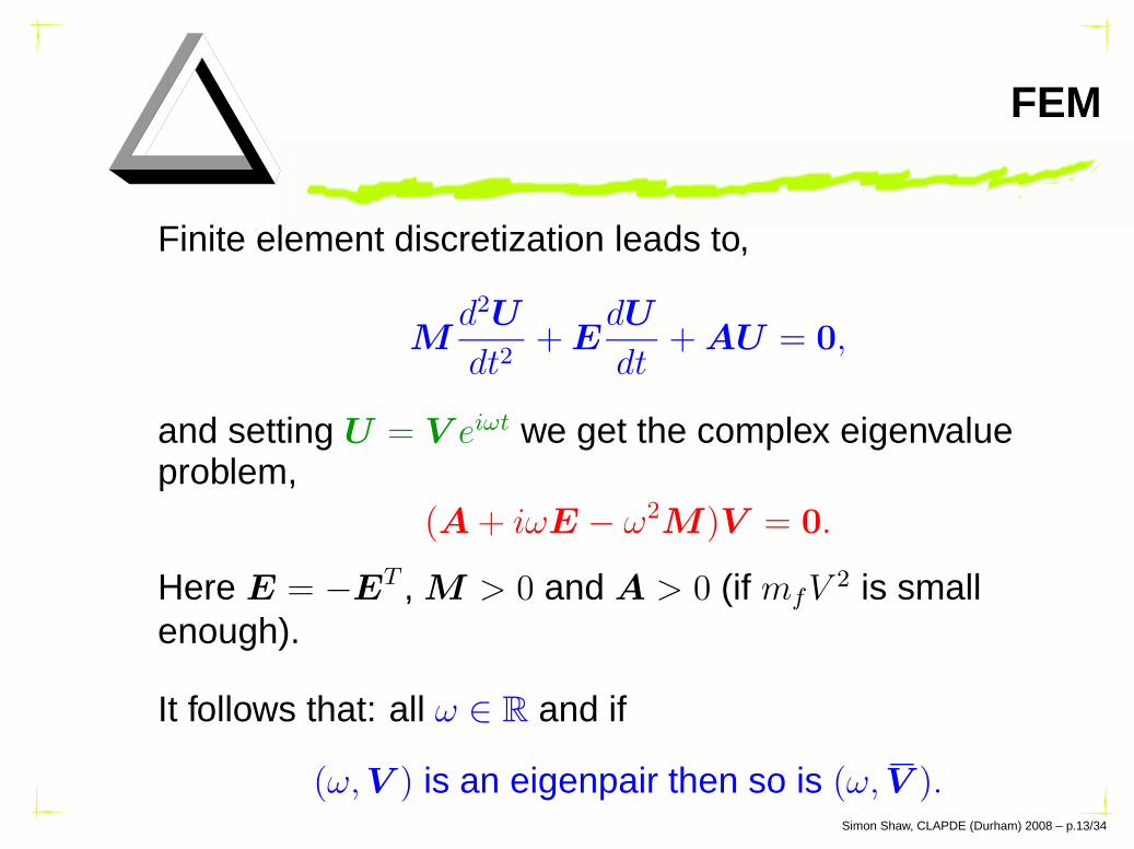
FEM

Finite element discretization leads to,

Md2U

dt2+ E

dU

dt+ AU = 0,

and setting U = V eiωt we get the complex eigenvalueproblem,

(A + iωE − ω2M)V = 0.

Here E = −ET , M > 0 and A > 0 (if mfV

2 is smallenough).

It follows that: all ω ∈ R and if

(ω,V ) is an eigenpair then so is (ω,V ).Simon Shaw, CLAPDE (Durham) 2008 – p.13/34

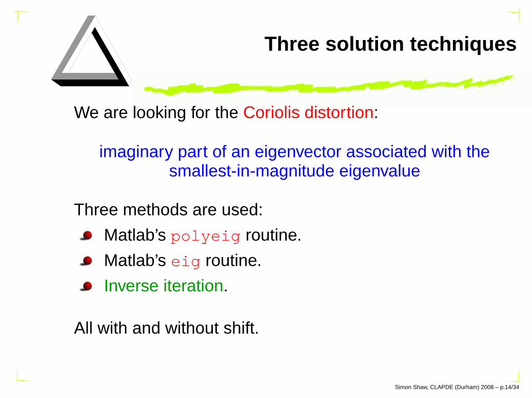
Three solution techniques

We are looking for the Coriolis distortion:

imaginary part of an eigenvector associated with thesmallest-in-magnitude eigenvalue

Three methods are used:

Matlab’s polyeig routine.

Matlab’s eig routine.

Inverse iteration.

All with and without shift.


polyeig for (A + iωE − ω2M)V = 0

The MATLAB fragment

[X, e] = polyeig(A, i * E, -M);

solves the quadratic eigenvalue problem in terms of acolumn of eigenvalues, e, and a matrix of eigenvectors, X.(Recall that A and M are invertible.)


eig for (A + iωE − ω2M)V = 0

Set W = ωV so that −ω2MV = −ωMW . Then:(

0 I

M−1

A iM−1E

)(

V

W

)

= ω

(

V

W

)

.

Hence: BX = XL, with L = diagonal of eigenvalues andX = eigenvectors. Solve in MATLAB via the fragment,

B = [ zeros(N,N) eye(N) ;M\A i * M\E ];

[X L] = eig(B);

(where A, E and M are N × N ).


Inverse iteration

Given D > 0 and x0 the iteration:

zn+1 = D−1

xn for n = 0, 1, 2, . . .

xn+1 = zn+1‖zn+1‖−1∞

converges to the eigenvector of the eigenvalue of leastmodulus of D (if this is well-defined).

For our system this is,

W n+1 = V n

V n+1 = A−1 (MW n − iEW n+1)

and we take (1 + 10−5i, 1 + 10−5i, . . .) as the initial guess.Simon Shaw, CLAPDE (Durham) 2008 – p.17/34

Summary

These methods were used with and without shift.

The physical constants in the PDEs are ‘real life’ andcorrespond to a real straight-tube meter.

Most meters are far more complicated in terms of designand geometry.

Before the numerics here is the background.


Collaboration and background

Robert Cheesewright (Engineering, Brunel) was gettingincorrect eigenvectors from ANSYS.

He asked for my help and advice in terms of FEM and‘locking’.

My independent C++ and matlab computations still gaveincorrect results. . .

The Timoshenko beam results are shown

The Euler-Bernoulli results are essentially the same

The results for a straight tube meter are. . .


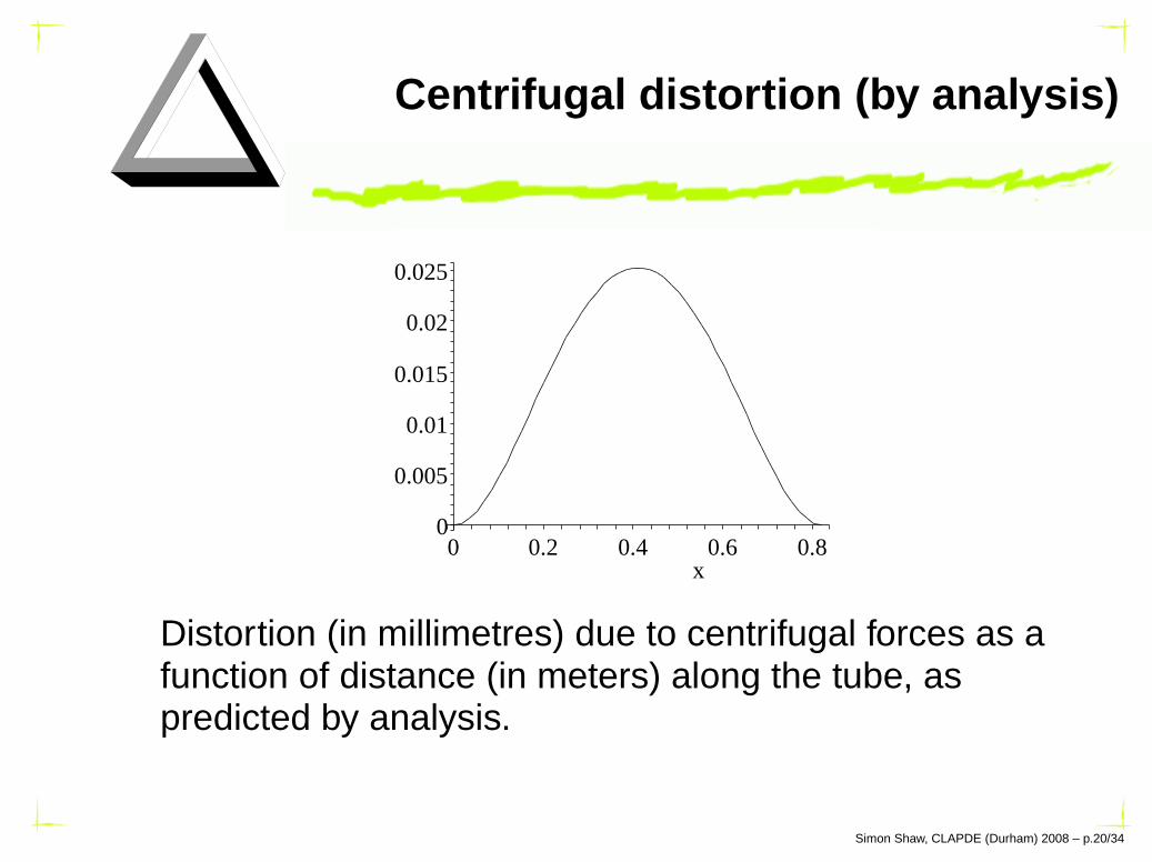
Centrifugal distortion (by analysis)

x

0.02

0.015

0.01

0.005

00.80.60.40.20

0.025

Distortion (in millimetres) due to centrifugal forces as afunction of distance (in meters) along the tube, aspredicted by analysis.


Coriolis distortion (by analysis)

0.04

x

0.02

00.8

-0.02

-0.04

0.60.40.20

Distortion (in millimetres) due to Coriolis forces as afunction of distance (in meters) along the tube, aspredicted by analysis.


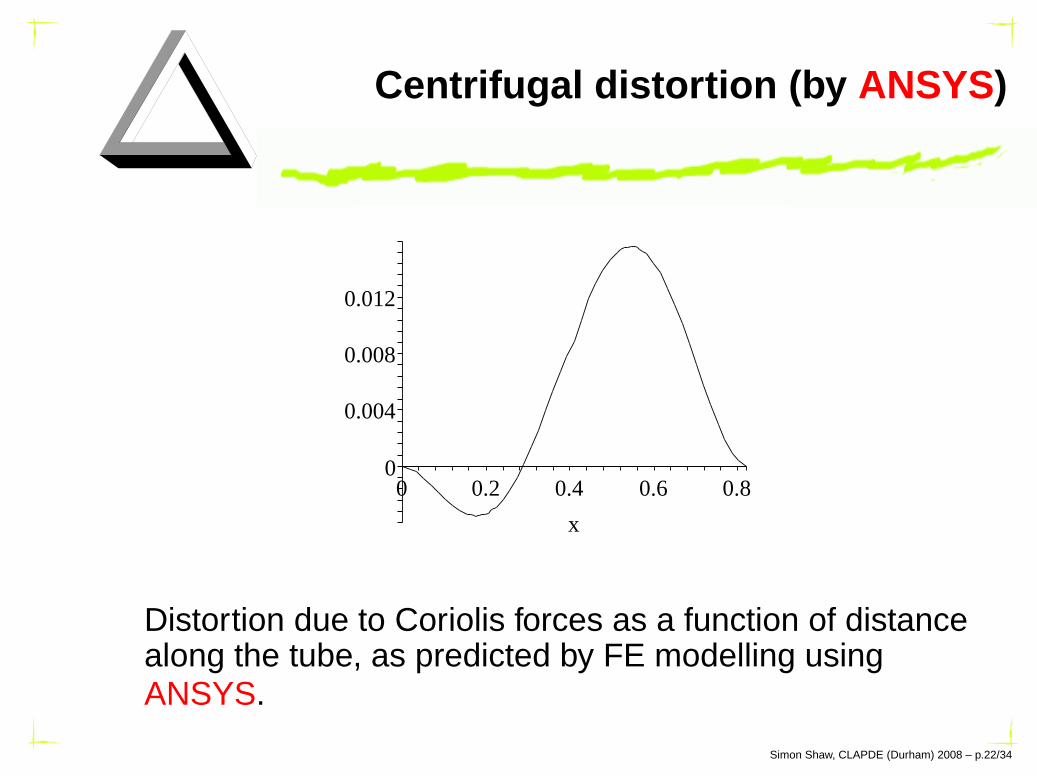
Centrifugal distortion (by ANSYS)

0.012

0.008

x

0.004

00.80.60.40.20

Distortion due to Coriolis forces as a function of distancealong the tube, as predicted by FE modelling usingANSYS.


My efforts. . .

The coriolis distortion is wrong and not physical.

My efforts:

C++ code to generate FE matrices

Data read by matlab for eigen-computations

The results were. . .


Eigenvalues (no shift)

|ω|min by technique. . .Ne 1 2 316 940.1753 940.1753 ≈ 1 ↔ 13000

32 938.9266 938.9266 ≈ 1 ↔ 13000

64 938.8359 938.8359 ≈ 1 ↔ 13000

128 938.8298 938.8300 ≈ 1 ↔ 13000

256 938.8296 938.8296 ≈ 1 ↔ 13000

Computed |ω|min for the Timoshenko beam (quadraticelements) with no shift, p = 0.


Eigenvalues (with shift)

|ω|min by technique. . .Ne 1 2 316 940.1753 940.1753 940.1753

32 938.9266 938.9266 938.9266

64 938.8359 938.8359 938.8359

128 938.8300 938.8300 938.8300

256 938.8296 938.8296 938.8296

Computed |ω|min for the Timoshenko beam (quadraticelements) with shift p = 900.


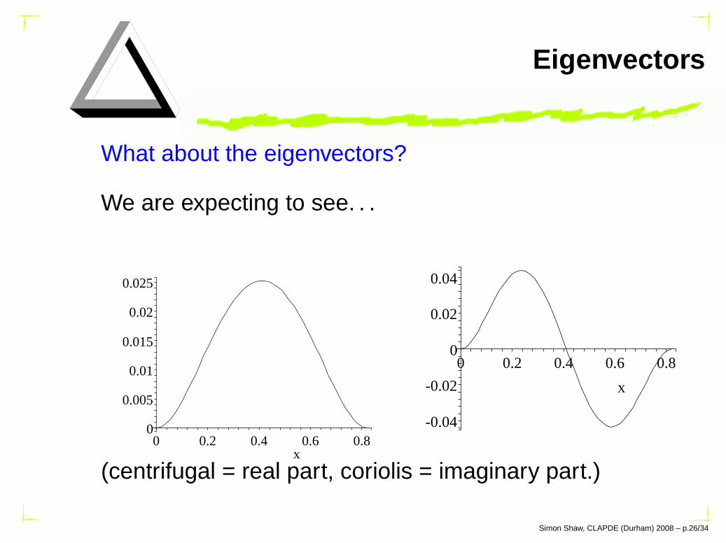
Eigenvectors

What about the eigenvectors?

We are expecting to see. . .

x

0.02

0.015

0.01

0.005

00.80.60.40.20

0.025 0.04

x

0.02

00.8

-0.02

-0.04

0.60.40.20

(centrifugal = real part, coriolis = imaginary part.)


polyeig without shift

0 0.2 0.4 0.6 0.8 10

0.1

0.2

0.3

0.4

0.5

0.6

0.7

0.8

0.9

1

x

Re

V (

norm

aliz

ed to

1)

0 0.2 0.4 0.6 0.8 10

0.05

0.1

0.15

0.2

0.25

x

Im V

(no

rmal

ized

on

Re

V)

ReV and Im V from Matlab’s eig routine. No shift (32elements).


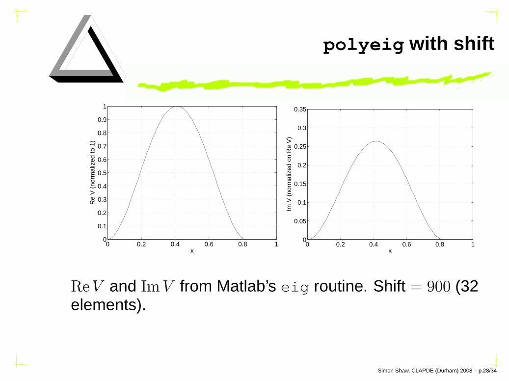
polyeig with shift

0 0.2 0.4 0.6 0.8 10

0.1

0.2

0.3

0.4

0.5

0.6

0.7

0.8

0.9

1

x

Re

V (

norm

aliz

ed to

1)

0 0.2 0.4 0.6 0.8 10

0.05

0.1

0.15

0.2

0.25

0.3

0.35

x

Im V

(no

rmal

ized

on

Re

V)

ReV and Im V from Matlab’s eig routine. Shift = 900 (32elements).


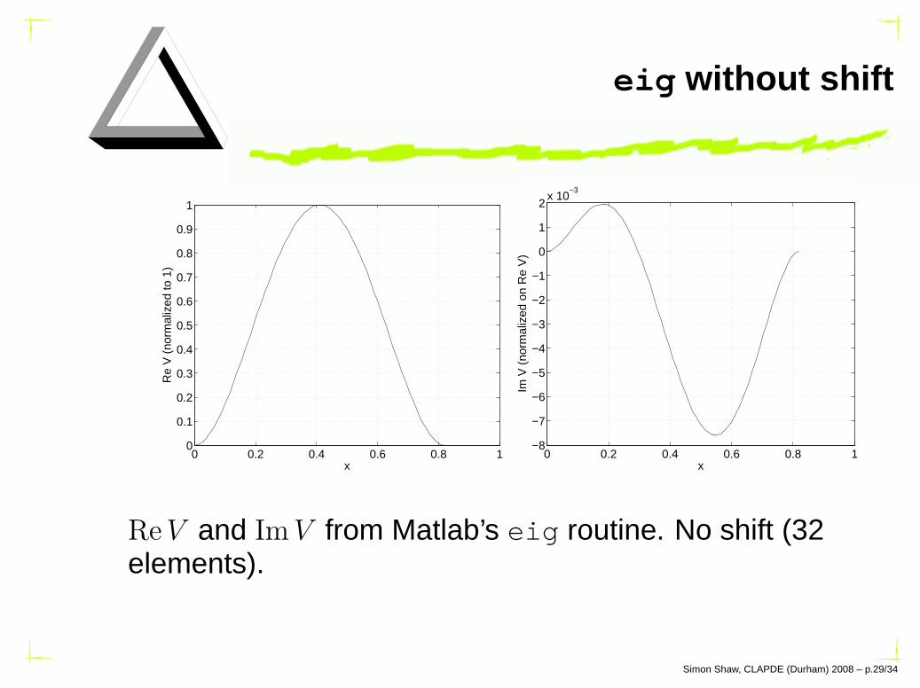
eig without shift

0 0.2 0.4 0.6 0.8 10

0.1

0.2

0.3

0.4

0.5

0.6

0.7

0.8

0.9

1

x

Re

V (

norm

aliz

ed to

1)

0 0.2 0.4 0.6 0.8 1−8

−7

−6

−5

−4

−3

−2

−1

0

1

2x 10

−3

x

Im V

(no

rmal

ized

on

Re

V)

ReV and Im V from Matlab’s eig routine. No shift (32elements).


eig with shift

0 0.2 0.4 0.6 0.8 10

0.1

0.2

0.3

0.4

0.5

0.6

0.7

0.8

0.9

1

x

Re

V (

norm

aliz

ed to

1)

0 0.2 0.4 0.6 0.8 1−8

−7

−6

−5

−4

−3

−2

−1

0

1

2x 10

−3

x

Im V

(no

rmal

ized

on

Re

V)

ReV and Im V from Matlab’s eig routine. Shift = 900 (32elements).


Inverse iteration without shift

0 0.2 0.4 0.6 0.8 10

0.1

0.2

0.3

0.4

0.5

0.6

0.7

0.8

0.9

1

x

Re

V (

norm

aliz

ed to

1)

0 0.2 0.4 0.6 0.8 1−2

0

2

4

6

8

10

12

14x 10

−6

x

Im V

(no

rmal

ized

on

Re

V)

ReV and Im V from inverse iteration. No shift (32elements).


Inverse iteration with shift

0 0.2 0.4 0.6 0.8 10

0.1

0.2

0.3

0.4

0.5

0.6

0.7

0.8

0.9

1

x

Re

V (

norm

aliz

ed to

1)

0 0.2 0.4 0.6 0.8 1−5

−4

−3

−2

−1

0

1

2

3

4

5x 10

−3

x

Im V

(no

rmal

ized

on

Re

V)

ReV and Im V from inverse iteration. Shift = 900 (32elements).


Conclusion

Shifted inverse iteration is most robust (given a goodinitial guess).

ANSYS and matlab seem to struggle.

Problem is due to rounding error (a hunch!)ω2r and 2ωV are different orders of magnitude.

A challenge for eigen-solvers?

. . . or is there an ‘easy’ remedy?


FIAM

I’ll leave you with the fundamental inequality of appliedmathematics:

‖T − P‖T ≪ ‖T − P‖P


FIAM


‖T − P‖T ≪ ‖T − P‖P

The difference between theory and practice in theoryis less than

the difference between theory and practice in practice.Anon, circa 20th Century


FIAM


‖T − P‖T ≪ ‖T − P‖P

The difference between theory and practice in theoryis less than

the difference between theory and practice in practice.Anon, circa 20th Century

The End. . .


Difﬁculties in computing the fundamental distortion mode in...

Documents

Transcript of Difﬁculties in computing the fundamental distortion mode in...