Diffusion in Multi-Component Liquids: from

Microscopic to Macroscopic Scales

G. Guevara-Carrion,† Y. Gaponenko,‡ T. Janzen,† J. Vrabec,† and V.

Shevtsova∗,‡

†Thermodynamics and Energy Technology, University of Paderborn, 33098 Paderborn, Germany

‡Microgravity Research Center, Université Libre de Bruxelles (ULB), CP–165/62, Av. F.D.

Roosevelt, 50, B–1050 Brussels, Belgium

E-mail: vshev@ulb.ac.be

Phone: +32 2 650 65 70

1

Abstract

In spite of considerable research on the nature of aqueous alcohol mixtures that are charac-

terized by microscopic inhomogeneity or incomplete mixing at the molecular level, transport

properties have received little attention. We report the results of a study on diffusion in the

ternary mixture of water with two alcohols, i.e., water + methanol + ethanol, which is inves-

tigated on microscopic and macroscopic scales by means of molecular simulation and Taylor

dispersion experiments. A novel protocol is developed for the comparison of mutual diffu-

sion coefficients sampled by two fundamentally different approaches, which allows for their

critical analysis. Because of complex intermolecular interactions, given by the presence of

hydrogen-bonding, the analysis of transport processes in this mixture is challenging for not

only on the microscopic scale for simulation techniques but also on the macroscopic scale due

to unfavorable optical properties. Binary limits of the Fick diffusion matrix are used for vali-

dation of the experimental ternary mixture results together with the verification of the validity

of the phenomenological Onsager reciprocal relations. The Maxwell-Stefan diffusion coeffi-

cients and the thermodynamic factor are sampled by molecular simulation consistently on the

basis of given force field models. The protocol for the comparison of the results from both

approaches is also challenging because Fick diffusion coefficients of ternary mixtures depend

on the frame of reference. Accordingly, the measured coefficients are transformed from the

volume-averaged to the molar-averaged frame of reference and it is demonstrated that both ap-

proaches provide not only similar qualitative behavior along two concentration paths but also

strong quantitative agreement. This coordinated work using different approaches to study dif-

fusion in multi-component mixtures is expected to be a significant step forward for the accurate

assessment of cross diffusion.

Introduction

Mixtures of alcohol and water are particularly complex systems that are challenging from the point

of view of both simulation and experiment. In spite of considerable research into the nature of

alcohol-water mixtures at the molecular level there still seem to be few studies on their macroscopic

2

properties, particularly for ternary mixtures. Water and methanol are the two most prominent

hydrogen-bonding liquids and their mixture has consequently been the subject of many studies.

Thorough research was undertaken for the methanol-water mixture concerning the influence of

segregation, clustering and the resulting molecular structures mainly in the water-rich and water-

poor concentration ranges1–3.

Binary data on the Fick diffusion coefficient are relatively abundant, in fact, both tracer and mu-

tual diffusion coefficients of all binary subsystems of the present ternary mixture were measured

over the full composition range4–6. However, the presence of coupled diffusion makes mutual dif-

fusion measurements in ternary systems more complicated because four Fick diffusion coefficients

have to be determined from a signal for two components. Indeed, the first experimental verifica-

tion of the existence of cross diffusion was reported a hundred years later7 than experimental and

theoretical investigations of binary liquid mixtures8.

Analyses of diffusion problems are typically based on the assumption of a binary system, i.e.,

either the mixture actually contains only two components, or, for dilute multicomponent systems,

only binary pairs are considered. However, in general, the concentration profiles cannot be ac-

curately modeled by means of binary analysis, and multicomponent diffusion equations are a ne-

cessity9. Hence, there is great interest in the improvement of experimental methodologies and in

the development of reliable methods for the prediction of mutual diffusion coefficients of mixtures

containing three or more components.

Owing to the rapid development of computing power, molecular modelling and simulation has

emerged as a powerful tool to complement experimental efforts10. Force field-based simulation

methods can contribute to the understanding and interpretation of experimental results, to obtain

predictive estimates and to inter- or extrapolate experimental data into regions that are difficult to

access in the laboratory11. Experimentally, the Fick diffusion coefficient can be measured on the

basis of a variety of techniques from optical interferometry to NMR spin relaxation. In the present

work, Taylor dispersion, also known as peak broadening technique, was employed.

Molecular simulation studies on diffusion coefficients of complex liquid mixtures containing

3

three or more components are almost absent. Liu et al.12 consistently predicted the Fick diffusion

coefficients of the ternary mixture chloroform + acetone + methanol, however, they were not able

to verify their results due to the lack of experimental data. The ternary mixture water + methanol

+ ethanol was also studied by Liu et al.13 by means of equilibrium molecular dynamics (EMD)

simulation, but solely in the region of infinite dilution. In most cases EMD has been employed to

predict the dynamic properties of aqueous solutions of methanol14–17 or ethanol14,17–20.

To the best of our knowledge, the diffusivity of the ternary mixture water + methanol + ethanol

has not been studied by experiment before. In a preceding work6 on that ternary mixture, the

mutual diffusion coefficients of all binary subsystems were predicted in a consistent manner, i.e.,

the Maxwell-Stefan diffusion coefficients and the thermodynamic factor matrix were obtained by

means of molecular simulation. Pronounced minima of the mutual diffusion composition depen-

dence for the strongly non-ideal binary subsystems water + methanol and water + ethanol were

accurately predicted. For the ternary mixture water + methanol + ethanol, a few data points were

predicted as well, but could not be assessed on the basis of experimental data at that time. One of

the aims of this work is to complement that effort, comparing simulations with experiments over

the whole composition range.

This study is the first to combine molecular simulation and experiment to determine diffusion

coefficients of a ternary mixture comprising water and two alcohols with low molar mass, i.e.,

water + methanol + ethanol. The paper is organized as follows. First, a brief explanation of the

general equations governing diffusive fluxes in ternary mixtures is given. Second, the experimental

methodology is described in detail, followed by a brief outline of the employed simulation tech-

niques. Subsequently, the experimental and simulation results for the Fick diffusion coefficient

matrix are presented, analyzed and compared with each other. The predicted intra-diffusion coeffi-

cients are also studied in the light of the microscopic structure of the mixture. Finally, conclusions

are drawn.

4

General description of diffusion

Fick’s law is the most common approach to describe mass transport in liquid mixtures. It relates

a mass flux to a gradient of its driving force21. When the driving force is expressed in terms of

the gradient of molar concentration ∇C j, the diffusive molar flux of component i in the volume-

averaged frame of reference JVi for a mixture containing N components is written as

JVi =−

N−1

∑j=1

DVi j∇C j , (i = 1, . . . ,N−1) . (1)

If the driving force is expressed in terms of the gradient of mole fraction ∇x j, the diffusive molar

flux JMi in the molar-averaged frame of reference is

JMi =−ρ

MN−1

∑j=1

DMi j ∇x j , (i = 1, . . . ,N−1) , (2)

where ρM is the molar density of the mixture. Because the molar fluxes depend on the choice

of a frame of reference, the diffusion coefficients are defined accordingly. The Fick diffusion

coefficients in the volume- and molar-averaged frames of reference are denoted by DVi j and DM

i j ,

respectively.

The Fick approach involves N−1 independent diffusion fluxes and a (N−1)× (N−1) matrix

of diffusion coefficients, which is generally not symmetric, i.e., Di j 6= D ji. The main diffusion

coefficients Dii connect the flux of component i to its own concentration gradient, while the cross

diffusion coefficients Di j describe the coupled flux of component i induced by the concentration

gradient of component j22. Numerical values of Di j depend both on the frame of reference for

velocity (molar-, mass- or volume-averaged) and on the order of the components.

In the present simulations the molar-averaged frame of reference was used to obtain the Fick

diffusion coefficients, where the following holds

N

∑i=1

JMi = 0 . (3)

5

On the other hand, the mathematical model of the Taylor dispersion technique in ternary mixtures

was originally developed for the volume-averaged frame of reference23. Here, the sum of fluxes is

defined as

N

∑i=1

JVi vi = 0 , (4)

where vi is the partial molar volume of component i in the mixture.

The diffusion coefficient matrix in the volume-averaged frame of reference DV obtained ex-

perimentally from the Taylor dispersion technique can be transformed into its form in the molar-

averaged frame of reference DM in order to be compared with the diffusion coefficient matrix

obtained from EMD by21

[DM] = [BuV ][DV ][BVu], (5)

where the elements of the matrices are given by

BVuik = δik− xi (vk− vN)/v,

BuVik = δik− xi (1− vk/vN) , (6)

δi j stands for the Kronecker delta function and

v =N

∑i=1

xivi. (7)

The required partial molar volume vi can be calculated straightforwardly from the partial molar

excess volume vEi given by24

vEi = vE−

N

∑k 6=i

xk

(∂vE

∂xk

)T,p,x j 6=i,k

, (8)

6

which was done here on the basis of experimental literature data25.

There are two approaches for the selection of the component order: one is based on the molar

mass and the other one on the density of the components in their pure state. In EMD the use of

molar mass is appropriate and the components with a higher (or lower) molar mass are typically

chosen as the independent ones. Hydrodynamic effects become important when liquid mixtures

are studied on a macroscopic scale. Thus, for experimental work, it is appropriate to choose the

components with the higher density in their pure state as the independent ones. Following the

latter convention, water and methanol were chosen as the independent components for the present

analysis of water (1) + methanol (2) + ethanol (3). This order corresponds to increasing molar

mass, cf. Table 1.

Diffusion in multicomponent mixtures can also be described by Maxwell-Stefan (MS) theory.

Here, the driving force is expressed in terms of the gradient of the chemical potential ∇µi, which

is assumed to be balanced by a friction force that is proportional to the mutual velocity ui− u j

between the components21

N

∑j 6=i=1

x j(ui−u j)

Ði j=−β∇µi , (9)

where β = 1/(kBT ) is the Boltzmann factor. The MS diffusion coefficient Ði j thus plays the role

of an inverse friction coefficient between components i and j. MS diffusivities are symmetric, i.e.,

Ði j = Ð ji, so that there are only N(N−1)/2 independent MS diffusion coefficients.

Because Fick’s law and MS theory describe the same phenomenon, a relation between both

sets of diffusion coefficients exists21

DM = B−1ΓΓΓ , (10)

in which all three symbols represent (N−1)×(N−1) matrices. DM is the matrix of Fick diffusion

coefficients in the molar-averaged frame of reference DMi j , where the elements of the matrix B are

defined by26

7

0.0 0.2 0.4 0.6 0.8 1.00.0

0.2

0.4

0.6

0.8

1.00.0

0.2

0.4

0.6

0.8

1.0

1 2 3 4 5 6 7 8 9

10

11

12

13

14

15

16

17

18

19

w2 / kg kg -1w 3

/ kg

kg-1

w1 / kg kg -1

Path B

Path

A

a)

Path B

0.0 0.2 0.4 0.6 0.8 1.00.0

0.2

0.4

0.6

0.8

1.00.0

0.2

0.4

0.6

0.8

1.0

1 23

4 5 67

8 9

10

11

12

13

14

15

16

17

18

19

x2 / m

ol mol -1x 3

/ m

ol m

ol-1

x1 / mol mol -1

Path

A

b)

Figure 1: Concentration matrices in mass (a) and mole (b) fractions for the mixture water (1) + methanol (2) +ethanol (3). The squares represent the state points for which Fick diffusion coefficients were measured, indicatingtheir running number. Poor optical properties were encountered in the shaded composition range.

Bii =xi

ÐiN+

N

∑j 6=i=1

x j

Ði j, Bi j =−xi

(1

Ði j− 1

ÐiN

), (11)

and the matrix of the thermodynamic factor ΓΓΓ is given by

Γi j = δi j + xi∂ lnγi

∂x j

∣∣∣∣T,p,xk,k 6= j=1...N−1

, (12)

where γi stands for the activity coefficient of component i. In this way, the MS diffusion coefficients

can be transformed to the Fick diffusion coefficients and vice versa, if the thermodynamic factor

matrix is known.

The MS approach separates mass transfer dynamics from thermodynamics, which is consid-

ered by the thermodynamic factor. The MS diffusion coefficients are related to chemical potential

gradients and therefore cannot directly be measured in the laboratory. However, they can well be

sampled by EMD employing the Green-Kubo formalism or, alternatively, from the mean square

displacement. ΓΓΓ serves as a conversion factor between Fick and MS diffusion coefficients, there-

fore, its knowledge is necessary to determine Fick diffusion coefficient data on the basis of EMD.

The thermodynamic factor is usually estimated from experimental vapor-liquid equilibrium

(VLE) or excess enthalpy data27,28, employing an equation of state or an excess Gibbs energy GE

8

model, such as Margules, Wilson, NRTL or UNIQUAC. However, the resulting thermodynamic

factor may be a major source of uncertainty. I.e., it highly depends on the underlying thermody-

namic model28 and it corresponds only to the thermodynamic conditions under which VLE data

were measured. In recent years, there has been a growing effort to sample the thermodynamic

factor directly by molecular simulation, e.g., based on Kirkwood-Buff theory29–31 or free energy

perturbation methods to obtain the composition dependence of the chemical potential6,32,33. In this

work, the thermodynamic factor was calculated from the composition dependence of the chemical

potential at constant temperature and pressure by Monte Carlo (MC) simulation as described in

preceding work6.

Particle-based EMD simulations are typically conducted by specifying mole fractions xi. In

experiments it is preferred to deal with directly accessible concentration variables, i.e., mass frac-

tions wi. Previously it has been shown 34 that a transformation of the governing equations of the

Taylor dispersion technique, originally written in terms of molar concentration Ci, to mass fraction

wi does not change their functional form. Consequently, both mass and mole fraction units can be

found in this study. The connection between them and the molar concentration is given by

wi = xi Mi/M, wi =Ci Mi/ρ, xi =Ci M/ρ , (13)

where Mi is the molar mass of component i, M is the average molar mass of the mixture and ρ is

the mass density of the mixture.

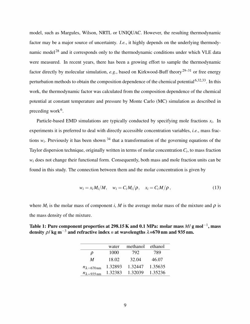
Table 1: Pure component properties at 298.15 K and 0.1 MPa: molar mass M/ g mol−1, massdensity ρ/ kg m−3 and refractive index n at wavelengths λ=670 nm and 935 nm.

water methanol ethanolρ 1000 792 789M 18.02 32.04 46.07

nλ=670nm 1.32893 1.32447 1.35635nλ=935nm 1.32383 1.32039 1.35236

9

Onsager reciprocal relations

Diffusion in multicomponent mixtures can also be described on the basis of irreversible thermo-

dynamics. Here, the Onsager matrix H, that relates the molar diffusive fluxes to the chemical

potential gradients, is defined. This formulation is equivalent to Fick and MS postulates so that21

B−1ΓΓΓ = DM = H−1G, (14)

where the elements of the symmetric Hessian matrix G are given by21

Gi j =∂ (µ j−µN)

∂xi= G ji. (15)

The matrix G can be obtained similarly as the thermodynamic factor matrix ΓΓΓ employing an equa-

tion of state or a GE model. Further, following the second postulate of irreversible thermodynam-

ics, the phenomenological Onsager matrix H is also symmetric, i.e, H = HT, which expresses the

Onsager reciprocal relations21.

The symmetry property of the matrices G and H restricts the values of the Fick diffusion matrix

DM. For a ternary mixture, Eq. (14) leads to a single relationship35

−G11DM12 +G12DM

11 =−G22DM21 +G21DM

22, (16)

so that there are only three independent Fick diffusion coefficients Di j21. Therefore, the restriction

given by Eq. (16) can be used as a consistency test for measured data35. For this purpose, a simple

method to evaluate the difference between both sides of Eq. (16), and therefore the degree of

asymmetry of the matrix DMG−1, has been proposed in the literature36

δOns(%) = 100%2(F1−F2)

(F1 +F2), (17)

where F1 and F2 correspond to the left and right hand sides of Eq. (16), respectively. δOns was

obtained here with the Fick diffusion coefficients in the molar-averaged frame of reference. The

10

matrix G was calculated employing the Wilson GE model fitted to experimental VLE data.

Ternary diffusion coefficients approaching binary limits

In this study, we had the unique opportunity to compare measured and simulated diffusion co-

efficients, nevertheless, for ternary mixtures an independent control of measurements is a neces-

sity. The behavior of ternary diffusion coefficients when approaching the binary limits provides

an efficient way for the validation of the experimental and simulation results. The asymptotic

behavior was previously developed for a mixture with vanishing excess volume, i.e., 1,2,3,4-

tetrahydronaphthaline (THN) + isobutylbenzene (IBB) + n-dodecane (C12)37, when the fluxes

can be written in a similar form in the volume-averaged and mass-averaged frames of reference.

Here we present a complete analysis of the asymptotic behavior of diffusion coefficients measured

by Taylor dispersion.

The two independent diffusive fluxes in the volume-averaged frame of reference (cf. Eq. (1))

can be written using mass fractions as

−JV1 /ρ =

1M1

DV11∇w1 +

1M2

DV12∇w2 , (18)

−JV2 /ρ =

1M1

DV21∇w1 +

1M2

DV22∇w2. (19)

When approaching the binary mixture at the bottom of the triangle in Fig. 1a, the content of w2

tends to zero as well as its mass flux, i.e., ∇w2→ 0 and JV2 → 0. Then, from Eq. (19) it follows

that D21→ 0, and from Eq. (18) it follows that D11→ Dw1−w3bin .

A similar analysis on the left hand side of the triangle, i.e., w1 → 0 provides that D12 → 0

and D22→ Dw2−w3bin . The behavior of the other diffusion coefficients cannot be predicted from this

analysis. Note that the asymptotic behavior in the limits w1→ 0 and w2→ 0 does not depend on

the frame of reference and coincides with the one reported previously37. However, the asymptotic

behavior on the right hand side of the triangle does depend on the frame of reference.

11

Following Fick’s law, the diffusive flux of the third component JV3 can be written as

JV3 =−(JV

1 v1 + JV2 v2)/v3 =

ρ

v3

[1

M1

(v1 DV

11 + v2 DV21)

∇w1 +1

M2

(v1DV

12 + v2DV22)

∇w2

]. (20)

Selecting the mass fractions of the second and third components as independent variables, it fol-

lows from the condition w1 +w2 +w3 = 1 that ∇w1 = −∇w2−∇w3 and the expressions for the

diffusive fluxes JV2 and JV

3 take the form

JV2 =−ρ

[(1

M2DV

22−1

M1DV

21

)∇w2−

1M1

DV21∇w3

], (21)

JV3 =

ρ

v3

{−[

1M1

(v1 DV

11 + v2 DV21)− 1

M2

(v1DV

12 + v2DV22)]

∇w2

}− ρ

v3

[1

M1

(v1 DV

11 + v2 DV21)

∇w3

]. (22)

Applying the same logic as above, from the conditions w3→ 0 and JV3 → 0 it follows that

DV22−

M2

M1DV

21 = Dw1−w2bin , (23)

and1

M1

(v1 DV

11 + v2 DV21)− 1

M2

(v1DV

12 + v2DV22)= 0. (24)

Indeed, the results from Ref.37 for the ideal mixture with equal molar masses are reproduced.

Experiments by Taylor dispersion

The Taylor dispersion technique is based on the diffusive spreading of a small volume of a solu-

tion injected into a laminar stream of the same mixture with a slightly different composition. As

the injected concentration pulse is carried through a tube, it is deformed by the coupled action of

convection in axial direction and diffusion in radial direction. At the end of the capillary, a refrac-

12

tive index detector monitors the concentration of the eluted peak (also known as Taylor peak) as

a function of time. The Fick diffusion coefficients are calculated from the resulting profile of the

refractive index variation.

A detailed description of the experimental set-up used in this study was published previ-

ously34,35,37, here only some practical information is provided. The inner diameter and length

of the polytetrafluoroethylene tube were 2R0 = 748± 1 µm and L = 29.839± 0.001 m, respec-

tively. The capillary was coiled around a grooved aluminum cylinder with a diameter of 30 cm

and was placed together with a refractometer and a pump in a temperature-regulated air bath at

298±0.2 K. The flow rate was 0.08 mL/min and the injected volume was ∆V = 20 µL.

The following substances were used without further purification: water pure from Acros Organ-

ics, deionized reagent Grade 3 (CAS Number: 7732-18-5), methanol of analytical reagent grade

from Fisher Scientific (CAS Number: 67-56-1) and ethanol absolute of analytical reagent grade

from VWR (CAS Number: 64-17-5).

The concentrations C1 and C2 at the end of the diffusion tube are given by the fundamental

working equations of Price23

Ci(t)−C0i =

2∆VR3U0

√3

π3t

(Ai1

√D1 exp(−D1η)

+Ai2

√D2 exp(−D2η)

), i = 1,2 , (25)

where η stands for 12(t − tR)2/R2t, C0i is the molar concentration of component i in the carrier

liquid and ∆V is the volume of the injected solution sample. The eigenvalues Di of the Fick

diffusion matrix Di j are given by

D1 =D11 +D22 +

√(D11−D22)2 +4D12D21

2, (26)

D2 =D11 +D22−

√(D11−D22)2 +4D12D21

2, (27)

13

and the coefficients Aik are defined as

A11 =(DV

22− D1)∆C1−DV12∆C2

D2− D1, (28)

A12 =(DV

22− D2)∆C1−DV12∆C2

−(D2− D1), (29)

A21 =(DV

11− D1)∆C2−DV21∆C1

D2− D1, (30)

A22 =(DV

11− D2)∆C2−DV21∆C1

−(D2− D1), (31)

where A11+A12 = ∆C1 and A21+A22 = ∆C2. Here ∆Ci = (Ci−C0i ) is the concentration difference

between injected sample and carrier liquid. Superscript V indicates that the measured Fick diffu-

sion coefficients correspond to the volume-averaged frame of reference. The eigenvalues do not

depend on the frame of reference and, correspondingly, there are no superscripts in Eqs. (26) and

(27).

The determination of four Fick diffusion coefficients DVi j experimentally by fitting is a notori-

ously difficult problem. One important issue is the selection of a proper initial guess. A promising

idea is to measure diffusion coefficients of ternary mixtures along a concentration path, starting

with a binary subsystem and moving towards another one. This creates a positive feedback loop:

the initial guess can be taken from a preceding state point, which, in turn, can be checked by the

continuity of the diffusion coefficient data. Measurements of single state points may lead to fitting

problems and even to an inversion of the numerical values of the main elements of the diffusion

matrix37–39. Fig. 1 presents the chosen paths in terms of mass and mole fractions: path A corre-

sponds to a constant mass fraction of water (w1=0.1 kg kg−1) and path B corresponds to a constant

mass fraction of methanol (w2=0.44 kg kg−1).

14

Optical properties of the mixture

The refractive index detector provides an electrical voltage signal V (t) which is assumed to be

linearly proportional to small concentration changes of all components of the mixture40

V (t) =m

∑i=0

ζi t i +[R1(w1(t)−w01)]+ [R2(w2(t)−w0

2)] , (32)

where Ri = ∂V/∂wi is the sensitivity of the detector to component i. This linear dependence

assumes small concentration differences ∆wi between injected sample and carrier liquid. The first

term in Eq. (32) compensates the drift of the detector baseline which was modeled by a polynomial

fit of order m, usually m=2.

The sensitivity Ri depends on the optical properties of the mixture, i.e., on the variation of the

refractive index with concentration ∂n/∂Ci (contrast factor) at the wavelength of the detector

Ri = ∂V/∂wi = (∂V/∂n)(∂n/∂wi) , (33)

where (∂V/∂n) is a constant of the detector. The ratio of contrast factors, the so called sensitivity

ratio SR, contributes substantially to the accuracy of Taylor measurements for a given system

SR =

(∂n

∂w1

)w2

/

(∂n

∂w2

)w1

. (34)

Note that the optical sensitivity depends on the concentration units34, i.e., SR(C) = SR(w)M1/M2.

We were aware of the difficulties using the Taylor dispersion technique for systems containing

water and methanol from a study on water + methanol + acetone due to unfavorable relative de-

tector sensitivity41. Keeping this in mind, two different approaches for the accurate determination

of contrast factors were used: measuring the refractive index at the wavelength of the detector as

well as calculating it from the peak area and the injected amount. Taylor peaks were detected by

a Knauer Smartline RI Detector 2300 which operates at the wavelength λ = 950 nm. Literature

data for the contrast factors at wavelengths λ > 900 nm are available only for a limited number

15

of ternary mixtures42–44. Thus, the refractive index at the nearest available wavelength λ=935 nm

and, for reference, at λ=670 nm was measured.

�����������

��

�� �� � �� �� ��

�

� �

�

�

� �

� �

� �

����� �����

����������

��

�����������

��

��� ��� �� �� ��� ��� ��

�

��

���

����

���

����

���

����

���������

���� �����

��

Figure 2: Measured refractive index of the mixture water (1) + methanol (2) + ethanol (3) as a function of massfraction at different wavelengths for a constant mass fraction of water w1 = 0.1 kg kg−1 (path A) and w2 = 0.44 kgkg−1 (path B). Note the difference in the vertical scales.

The measured refractive index along paths A and B is listed in Table 2 and presented in Fig. 2.

Along path A the curves n(w2) at different wavelengths reveal nearly parallel lines over the entire

concentration space and, as expected, with the increase of λ the refractive index decreases. The

measured data n(w2) along path A were interpolated by a linear function as seen in Fig. 2a, and

the contrast factors are (∂n/∂w2)w1,λ=935nm = -0.0322 and (∂n/∂w2)w1,λ=670nm = -0.0328. For

validation of the measurements, the values of n at the binary limits in the case of λ=670 nm were

favorably compared with literature data.

Fig. 2b presents the variation of the refractive index along path B. The much weaker depen-

dence of n(w1) at both wavelengths has a similar shape, displaying a maximum. The measured

n(w1) data were interpolated by a suitable function and its differentiation provided the contrast

factor (∂n/∂w1)w2 which decreases with concentration w1 at both wavelengths. In particular, this

derivative changes its sign in the vicinity of state point #4, which occurs at w1=0.179 kg kg−1 for

λ=935 nm and w1=0.215 kg kg−1 for λ=670 nm. This region with poor optical properties along

path B is shaded in Fig. 1a. Moving to the apex of the composition triangle, the location of the

vanishing derivative is shifted to smaller concentrations of water. Finally, the sensitivity ratio SR

16

Table 2: Measured refractive index of the mixture water (1) + methanol (2) + ethanol (3) attwo different wavelengths λ for a constant mass fraction of water w1 = 0.1 kg kg−1 (path A)and w2 = 0.44 kg kg−1 (path B).

Path APoint # w2 nλ=670nm nλ=935nm

10 0 1.35956 1.3548011 0.1 1.35597 1.3515812 0.17 1.35362 1.3493113 0.25 1.35070 1.3467814 0.37 1.34704 1.3430715 0.5 1.34270 1.3387916 0.6 1.33972 1.3359717 0.7 1.33711 1.3329518 0.8 1.33291 1.3287719 0.9 1.32949 1.32529

Path BPoint # w1 nλ=670nm nλ=935nm

1 0 1.3433 1.34013 0.1 1.3451 1.34115 0.25 1.3456 1.34166 0.3 1.3456 1.34107 0.4 1.3436 1.33928 0.5 1.3407 1.3367

17

was used as a fitting parameter in a small region around the originally measured values.

Selection of injected samples

We have experience in subtracting data from the measured peaks in ternary mixtures34,35,37. How-

ever, for the present mixture we faced a severe problem with the fitting procedure for some state

points along both paths. Rather often the solution converged to a set of diffusion coefficients which

did not correspond to the asymptotic predictions37. In this section we discuss the handling of the

region with poor optical properties using a diverse selection of injected samples.

�����������

��

��� ��� ���� ���� ����

������������

���

���

�� �

�� �

�� �

� ��� ��� ���� ��

�

������������������

������������

��� �� �� � � ��

�����

�

��

�

��

��

��������������������������������

��

Figure 3: (a) Diffusion couples, i.e., concentration of the carrier liquid (point P) and injected samples used in theexperiments measuring diffusion coefficients at state point #15 of the mixture water (1) + methanol (2) + ethanol (3);(b) Ternary dispersion profile and fitting curve in the ternary mixture with injected sample 15.1.

The typical protocol for the selection of injections is the following: a first sample is injected

with ∆w1 = 0, a second one with ∆w2 = 0 and a complimentary one where both mass fractions

are non-zero. From Eq. (32) it follows that due to the smallness of the derivative, i.e., R1, the net

variation of the refractive index ∆n can be very low for the injection with ∆w2=0. Thus, we rely

on the injections with non-zero diffusion couples, i.e., when ∆w1 6= 0 and ∆w2 6= 0 simultaneously.

Schematically, the considered injected samples for state point #15 are presented in Fig. 3a. Non-

perpendicular injections very often lead to a peak with dips as shown in Fig. 3b. Our code can

treat such peaks satisfactorily. E.g., a stable solution for state point #15 was obtained using simul-

taneous fitting of the four peaks obtained with injections 15.2 and 15.4; all of them were repeated

18

twice. Each peak was initially treated as a binary mixture and pseudo-diffusion coefficients were

determined. The peak quality was controlled by the reproducibility of the pseudo-diffusion coef-

ficients. For this purpose, the experiment with the same injection was repeated up to four times.

The number of injected samples varied between four and six, depending on fitting convergence.

Furthermore, when both concentrations are changed in an injection, the derivatives (∂n/∂wi)w j ,

(i 6= j) change values as the quantity in the subscript w j is not constant anymore. We have found

out that by varying ∆wi it is possible to find combinations of Taylor peaks with slightly better

optical sensitivity such that the fitting procedure converges better.

Fitting procedure

An unconstrained Nelder-Mead (simplex) method available in Matlab, similar to that employed by

Mialdun et al.35, was used for the fitting of experimental refractive index detector voltage data with

working equations. Instead of direct fitting of the coefficients DV11, DV

12, DV21 and DV

22, the procedure

suggested by Ray and Leaist45 was used. A peak signal was normalized such that Eq. (32) takes

the form

V (t) =m

∑i=0

ζi t i +∆Vmax

√tRt

[W1exp(−D1η)+(1−W1)exp(−D2η)

], (35)

where W1 is the normalized weight

W1 =(a+bα)

√D1

(a+bα)√

D1 +(1−a−bα)√

D2, (36)

and the parameters are

a =DV

11− D1−SR DV12

(D2− D1), (37)

b =DV

22−DV11−DV

21/SR +SR DV12

(D2− D1), (38)

α =∆w1

∆w1 +∆w2(M1/M2)/SR. (39)

19

The Fick diffusion coefficients were calculated from the fit parameters D1, D2, a and b as follows45

DV11 = D1 +

a(1−a−b)b

(D1− D2) , (40)

DV12 =

1SR

a(1−a)b

(D1− D2) , (41)

DV21 = SR

(a+b)(1−a−b)b

(D2− D1) , (42)

DV22 = D2 +

a(1−a−b)b

(D2− D1) . (43)

Note that there is a misprint of signs in Eq. (38) in the original paper45.

Molecular Simulation

The Fick diffusion coefficient matrix was determined consistently by means of molecular simula-

tion. I.e., both the MS diffusion coefficient and the thermodynamic factor matrices were computed

exclusively on the basis of simulation data. For this purpose, rigid, united-atom type models were

used to describe the intermolecular interactions. The molecular models employed in this work46–48

account for these interactions, including hydrogen-bonding, by a set of Lennard-Jones (LJ) sites

and point charges which may or may not coincide with the LJ site positions. The molecular mod-

els for methanol and ethanol were taken from prior work46,47. For water, the TIP4P/2005 model

by Abascal and Vega48 was used. These models were satisfactorily assessed in previous works

with respect to the binary subsystems of the ternary mixture under consideration6,14. The inter-

ested reader is referred to the original publications46–48 for detailed information about the three

molecular pure substance models and their parameters.

To define a molecular model for a ternary mixture on the basis of pairwise additive pure sub-

stance models, only the unlike interactions have to be specified. In case of polar interaction sites,

i.e., point charges here, this can straightforwardly be done using the laws of electrostatics. How-

ever, for the unlike LJ parameters, there is no physically sound approach so that combining rules

have to be employed for predictions. Therefore, the simple Lorentz-Berthelot combining rule was

20

chosen. Because not a single experimental data point on mixture properties or on transport prop-

erties was considered in the model parameterization, the mixture data from molecular simulation

presented below are strictly predictive.

Methodology

The Green-Kubo formalism based on the net velocity auto-correlation function26

Li j =1

3Np

∫∞

0dt⟨ Np,i

∑k=1

vi,k(0) ·Np,j

∑l=1

vj,l(t)⟩, (44)

was used here to calculate the MS diffusion coefficients. Np is the total number of molecules, Np,i

is the number of molecules of component i and vi,k(t) denotes the center of mass velocity vector

of the k-th molecule of component i at time t. Note that Eq. (44) corresponds to a reference frame

in which the mass-averaged mixture velocity is zero26.

For a ternary mixture, the elements of the inverse matrix B−1 in the molar-averaged frame of

reference, cf. Eqs. (10) and (11), are given by26

B−111 = (1− x1)

(L11

x1− L13

x3

)− x1

(L21

x1− L23

x3+

L31

x1− L33

x3

),

B−112 = (1− x1)

(L12

x2− L13

x3

)− x1

(L22

x2− L23

x3+

L32

x2− L33

x3

),

B−121 = (1− x2)

(L21

x1− L23

x3

)− x2

(L11

x1− L13

x3+

L31

x1− L33

x3

),

B−122 = (1− x2)

(L22

x2− L23

x3

)− x2

(L12

x2− L13

x3+

L32

x2− L33

x3

). (45)

The three MS diffusion coefficients can be calculated with

21

Ð13 =1

B11 +B12 · (x2/x1),

Ð12 =1

B11−B12 · (x1 + x3)/x1,

Ð23 =1

B22 +B21 · (x1/x2). (46)

During EMD simulation runs, the intra-diffusion coefficients were sampled simultaneously. The

corresponding Green-Kubo equation can be found, e.g., in Ref.6.

In the present work, the thermodynamic factor was calculated following its definition (12).

The chemical potentials, and thus the activity coefficients, were sampled by MC simulation on

the basis of the same molecular force field models. The derivatives of the activity coefficients at

constant temperature and pressure were subsequently obtained from a fit of the simulation results

using a thermodynamic model. Having the thermodynamic factor, the MS diffusion coefficients,

as determined by EMD, were transformed to the Fick diffusion coefficients according to Eq. (10).

Sampling the chemical potential by simulation is often a difficult task for dense liquids, re-

quiring advanced techniques. However, in previous work6 it was shown that with an appropriate

method and suitably chosen parameters, the composition profile of the chemical potential can be

obtained by relatively inexpensive MC simulations with at least the same precision as with the

method based on experimental VLE data.

The chemical potential µi of component i can be separated into the solely temperature depen-

dent ideal contribution µ idi (T ) and the remaining contribution µi(T, p,xxx) ≡ µi(T, p,xxx)− µ id

i (T ).

This contribution contains the desired lnγi term that appears in Eq. (12). In this way, the mole

fraction derivative of the activity coefficient can be written as

∂ lnγi

∂x j

∣∣∣∣T,p,xk,k 6= j=1...N−1

=∂ (β µi− lnxi)

∂x j

∣∣∣∣T,p,xk,k 6= j=1...N−1

. (47)

This derivative was calculated analytically from the Wilson model that was fitted to simulation

22

data. The thermodynamic factor is then given by28

Γi j = δi j + xi(Qi j−QiN) , (48)

and

Qi j =−Λi j/Si−Λ ji/S j +N

∑k=1

xkΛkiΛk j/S2k , (49)

where Si is a function of Λi j and composition. Λi j are adjustable Wilson parameters and their

numerical values are given in Ref.6. Note that this multicomponent thermodynamic model defines

also the properties of its binary subsystems.

Results and discussion

Experiment

The main elements of the Fick diffusion coefficient matrix monotonically grow with increasing

methanol content along path A, while DV11 < DV

22, as seen in Fig. 4a. The cross elements of the

diffusion matrix shown in Fig. 4b are negative and essentially smaller than the main terms; over

that path |DV12| is slightly larger than |DV

21|. A negative cross element of the diffusion matrix DVi j

implies that species i diffuses towards larger concentrations of species j.

The experiment was originated on path B (state point #1) and the fitting procedure for path A

began at the intersection of two paths, then it moved up and down. Unlike other mixtures34,37,

the convergence of the fitting routine deteriorates approaching the binary limits along path A. In

the limit w2→ 0 the cross diffusion coefficient DV21 should tend towards zero, whereas DV

11 should

reach the limit of the binary Fick diffusion coefficient of the water-ethanol subsystem Dw1−w3bin . Nu-

merous repetitions of the experiment at state point #11 provided two stable solutions: one of them

is indicated in Table 3 and the another one corresponds to similar eigenvalues (DV11=1.11; DV

12=-

0.017, DV21=-0.007; DV

22 =1.14 in units of 10−9m2/s). This ambiguity is in line with observations

23

for the binary mixture water-ethanol. The majority of experiments on binary diffusion in water-

ethanol with a mass relation 0.1/0.9 reported a diffusion coefficient of Dw1−w3bin = 0.88 ·10−9 m2/s34

which is shown as a blue diamond in Fig. 4a. However, there is another result Dw1−w3bin = 0.65 ·10−9

m2/s in the literature49 which is depicted in Fig. 4a as a blue open circle. Asymptotically, the for-

mer binary diffusion coefficient corresponds to the ternary system with similar eigenvalues and the

latter one to the ternary coefficients presented above. This indeterminacy can be attributed to re-

cent experimental studies on binary mixtures of concentrated low molar weight alcohols and water,

which have demonstrated incomplete mixing at the molecular level in alcohol-water systems1.

At the other end of the concentration path, i.e., w3 → 0, the observations are even more in-

triguing. The measured binary diffusion coefficient at state point #19 scattered in the range of

(1.75− 2.8) · 10−9 m2/s. The solution of that enigma becomes evident when one of the experi-

ments revealed a peak with dips, similar to that in Fig. 3b. Such a peak identifies two different

kinetics in the liquid system which are possible only in ternary or higher mixtures. Thus, our ex-

periment for the first time presented an evidence on the macroscopic scale that a binary system

may behave as a ternary system due to clustering.

The results of the Taylor dispersion measurements for the main diffusion coefficients DV11 and

DV22 along path B are shown in Fig. 5a. The open symbols indicate the asymptotic values of

the coefficient near the binary limits. The first observation at both ends of path B is that our

measurements perfectly meet the expectations at the binary limits. Indeed, the asymptotic quantity

derived in Eq. (23) is equal to [DV22−DV

21(M2/M1)] = 0.9 · 10−9m2/s, while the measured binary

diffusion coefficient on the right hand side (state point #9, w1=0.56 kg kg−1) is Dw1−w2bin = 0.94 ·

10−9m2/s. The second asymptotic quantity, expressed by Eq. (24), tends to zero and the coefficient

DV11 obtained from this expression is in excellent agreement with the measured value.

Near the binary limits, the reproducibility of the results was excellent in terms of the pseudo-

binary diffusion coefficients and convergence to the same solution regardless of the initial guess.

The calculated relative uncertainty, i.e., the standard deviation divided by the average value, yields

coherent results of about 2% which can be applied to mass fractions w1 < 0.1 kg kg−1 and w1 > 0.3

24

kg kg−1. However, along path B the uncertainty of the measured diffusion coefficients increases

due to the poor optical properties of the mixture discussed above. This region of poor contrast is

indicated by a shadow in Fig. 5.

The cross diffusion coefficients presented in Fig. 5b show a very different behavior along path

B: relatively large negative DV12 values and small DV

21 values that change sign in the middle of the

path. It is worth noting that in line with the asymptotic predictions, DV12→ 0 was found on the left

hand side of the triangle. Again, the coefficients are strongly dispersed around the trend curve in

the region with poor optical properties.

The numerical results for the diffusion coefficients measured by Taylor dispersion in the ternary

mixture are listed in Table 3.

��

�����������

���

���

���

���

���

��

��

��

��

�

���������

��

��� �� ��� ��� ��� ���

��

�����������

���

����

����

���

���

��

�

��

�

��

Figure 4: (a) Measured main elements DV11, DV

22 and (b) cross elements DV12, DV

21 of the Fick diffusion coefficientmatrix along path A in the mixture water (1) + methanol (2) + ethanol (3). The open symbols indicate asymptoticvalues approaching the binary subsystem from Ref.34 (circle) and Ref.49 (diamond). The dotted lines are given as aguide for the eyes.

25

Table 3: Measured Fick diffusion coefficients DVi j/10−9m2s−1 and their uncertainties

σ/10−9m2s−1 for the mixture water (1) + methanol (2) + ethanol (3) at 298.15 K and 0.1 MPaalong path A (w1 = 0.1 kg kg−1) and path B (w2 = 0.44 kg kg−1). The degree of asymmetryδOns (%) according to Eq. (17) is also given.

Point # w1 w2 w3 DV11 σ DV

12 σ DV21 σ DV

22 σ δOns

Path A

10 0.10 0.00 0.90 0.877 0.01811 0.10 0.10 0.80 0.762 0.199 -0.381 0.057 -0.237 0.088 1.055 0.165 -38.912 0.10 0.17 0.73 0.818 0.008 -0.320 0.058 -0.217 0.083 1.150 0.008 -5.213 0.10 0.25 0.65 0.971 0.047 -0.330 0.055 -0.280 0.045 1.120 0.032 -2.314 0.10 0.37 0.53 1.178 0.063 -0.273 0.115 -0.253 0.102 1.311 0.046 5.415 0.10 0.50 0.40 1.114 0.014 -0.238 0.027 -0.178 0.022 1.473 0.014 12.216 0.10 0.60 0.30 1.275 0.035 -0.222 0.014 -0.203 0.039 1.613 0.008 2.917 0.10 0.70 0.20 1.357 0.002 -0.300 0.046 -0.181 0.030 1.733 0.002 4.118 0.10 0.80 0.10 1.296 0.043 -0.300 0.051 0.048 0.018 1.939 0.007 5.319 0.10 0.90 0.00 2.250 0.430

Path B

1 0.00 0.44 0.56 1.6842 0.03 0.44 0.53 1.625 0.005 -0.040 0.052 -0.132 0.013 1.562 0.009 5.83 0.10 0.44 0.46 1.051 0.084 -0.189 0.098 -0.103 0.044 1.480 0.056 19.34 0.20 0.44 0.36 1.069 0.151 -0.594 0.156 -0.065 0.061 1.067 0.150 27.25 0.25 0.44 0.31 0.695 0.168 -0.630 0.134 0.083 0.030 1.351 0.133 45.66 0.30 0.44 0.26 0.745 0.019 -0.422 0.122 0.019 0.007 1.194 0.007 13.37 0.40 0.44 0.16 0.737 0.013 -0.359 0.078 0.038 0.011 1.116 0.010 4.18 0.50 0.44 0.06 0.639 0.016 -0.336 0.148 0.157 0.057 1.165 0.016 6.4

26

Table 4: Eigenvalues D1 and D2 in units of 10−9m2s−1 along path A (w1 = 0.1 kg kg−1) andpath B (w2 = 0.44 kg kg−1) at 298.15 K and 0.1 MPa from experiments and predicted bymolecular simulation.

Point # w1 w2 w3 Dexp1 Dexp

2 Dsim1 Dsim

2

Path A

11 0.10 0.10 0.80 1.243 0.574 1.103 0.75112 0.10 0.17 0.73 1.295 0.673 1.175 0.85313 0.10 0.25 0.65 1.358 0.733 1.198 0.85414 0.10 0.37 0.53 1.515 0.973 1.341 1.0243 0.10 0.44 0.46 1.522 1.010 1.393 1.018

15 0.10 0.50 0.40 1.567 1.021 1.434 1.12316 0.10 0.60 0.30 1.716 1.173 1.559 1.18917 0.10 0.70 0.20 1.845 1.246 1.592 1.25018 0.10 0.80 0.10 1.915 1.320 1.689 1.476

Path B

2 0.03 0.44 0.53 1.672 1.514 1.750 1.3263 0.10 0.44 0.46 1.522 1.010 1.393 1.0184 0.20 0.44 0.36 1.264 0.871 1.267 0.8705 0.25 0.44 0.31 1.260 0.787 1.237 0.8006 0.30 0.44 0.26 1.175 0.764 1.154 0.7827 0.40 0.44 0.16 1.076 0.777 1.089 0.7058 0.50 0.44 0.06 1.031 0.774 1.037 0.730

27

��

�����������

���

���

���

���

���

��

��

��

�� �

����������

��

��� ��� �� ��� ��� ��� ���

��

�����������

���

����

����

���

�����

�

��

���

Figure 5: (a) Measured main elements DV11, DV

22 and (b) cross elements DV12, DV

21 of the Fick diffusion coefficientmatrix along path B in the mixture water (1) + methanol (2) + ethanol (3). The open symbols indicate asymptoticvalues approaching the binary subsystem from present experiments. Poor optical properties were encountered in theshaded composition range. The dotted lines are given as a guide for the eyes.

28

Verification of the Onsager reciprocal relations

The experimental verification of the Onsager reciprocal relations (ORR) for ternary diffusion are

dated back to 196050. That examination was carried out on the basis of diffusion coefficient data

for ten different aqueous salt solutions (KCl, NaCl, LiCl) or raffinose. Since then, published data

on the experimental verification of ORR are rare. We have checked the validity of ORR at all mea-

sured state points, although the procedure is not straightforward. The diffusion coefficients were

measured in the volume-averaged frame of reference and then converted to the molar-averaged

frame of reference by Eq. (5). The required partial molar volumes and the thermodynamic matrix

G are known with some uncertainty which could influence the degree of asymmetry defined by

Eq. (17). The numerical values for these quantities are given in the Appendix B. Furthermore, it

was noted above that the measurement of diffusion coefficients at some state points of this mixture

was particularly difficult. Still, the correct qualitative behavior is expected to be captured.

The degree of asymmetry of the ORR is given in the last column of Table 3 and it follows that

the ORR are fulfilled within acceptable error limits. The value of the misfit is in accordance with

the quality of the results for the diffusion coefficients discussed above. Along path A the ORR are

satisfied within error limits smaller than 5.3% with the exception of state points #11 and #15. It

should be recalled that at the problematic state point #11 there is a second solution for which the

ORR are satisfied with δOns(%) = 0.25% and that state point #15 falls into the region where the

optical properties start to decline.

Along path B the ORR are satisfied within an error depending on the quality of the optical

properties of the mixture. The largest uncertainty was observed in the region with the poorest

optical contrast (state point #5) and then decreases down to 4%.

Simulation

Predictive molecular simulations were carried out at 298.15 K and 0.1 MPa along paths A and B

as depicted in Fig. 1. Moreover, 12 additional state points were sampled to cover the remaining

ternary composition range of the ternary liquid mixture.

29

The thermodynamic factor matrix was obtained from the Wilson GE model fitted to the chem-

ical potential data from molecular simulation using Eqs. (48) and (49). The systematic error in-

troduced by that fit was estimated to be less than 5% in magnitude. The MS diffusion coefficients

were obtained with EMD and the Green-Kubo formalism and the Fick diffusion coefficient matrix

based on the molar-averaged frame of reference was calculated using Eq. (10). The numerical sim-

ulation results for the predicted molar density, MS diffusion coefficients and the thermodynamic

factor matrices are listed in table 5 for all regarded state points. The Fick diffusion coefficient ma-

trix is given for paths A and B in table 6. All simulation results are consistent and their numerical

values for DM fulfill the theoretical restrictions for thermodynamic stability given by Taylor and

Krishna21, i.e., DM has positive and real eigenvalues, positive diagonal elements and a positive

determinant.

Usually, the main Fick diffusion coefficients DMii are larger than the cross elements DM

i j ( i 6= j),

which is expected as the diffusive flow of component i is mainly driven by its own concentration

gradient51. Coupling effects described by the relation between the diffusion coefficients DM21 and

DM22 are not important. On the other hand, the absolute numerical values of the cross diffusion

coefficient DM12 can be more important than the main term DM

11, especially for state points #7 and #8,

suggesting larger coupling effects, which may be caused by the presence of strong non-idealities.

Further, DM22 is always larger than DM

11, DM12 is negative throughout and DM

21 can be positive or reach

small negative values depending on mixture composition.

Fig. 6 shows a fit of the simulation results for the four Fick diffusion coefficients in the molar-

averaged frame of reference for the studied mixture over the whole composition range. As can

be seen, the surfaces for the four different coefficients behave differently. DM11 is always positive

but can achieve values up to six times lower than its maximum value. The values of DM22 exhibit a

smaller variation than that of DM11, reaching values only twice as low as their maximum. DM

21 varies

from positive to negative and DM21 is always negative.

Table 7 shows the comparison of the predictions made by molecular simulation here and in

previous work6. Although the same force field models were used, the values are not expected to be

30

Table 5: Molar density ρM / mol l−1, Maxwell-Stefan diffusion coefficients Ði j/10−9m2s−1

together with their statistical uncertainties σ/10−9m2s−1 and the thermodynamic factor ma-trix of the ternary system water (1) + methanol (2) + ethanol (3) at 298.15 K and 0.1 MPapredicted by molecular simulation.

x1 x2 x3 ρM Ð13 σ Ð12 σ Ð23 σ Γ11 Γ12 Γ21 Γ220.062 0.510 0.428 21.40 1.422 0.39 1.453 0.40 1.724 0.10 0.919 -0.021 -0.031 1.0320.190 0.469 0.341 23.84 1.223 0.29 1.457 0.44 1.298 0.14 0.760 -0.062 0.072 1.0570.340 0.421 0.239 27.40 1.271 0.27 1.634 0.54 1.025 0.17 0.588 -0.104 0.205 1.0860.404 0.400 0.196 29.20 1.282 0.27 1.530 0.47 1.023 0.19 0.520 -0.121 0.269 1.1000.462 0.381 0.157 31.04 1.371 0.30 1.661 0.55 0.827 0.18 0.461 -0.136 0.333 1.1140.563 0.349 0.088 34.82 1.292 0.32 1.708 0.75 0.695 0.20 0.368 -0.164 0.468 1.1430.649 0.321 0.030 38.72 1.435 0.44 1.653 0.80 0.619 0.26 0.300 -0.188 0.621 1.1780.213 0.120 0.667 21.22 1.044 0.13 1.040 0.44 1.092 0.17 0.718 -0.070 0.002 1.0220.208 0.199 0.593 21.76 1.154 0.18 1.282 0.52 1.096 0.15 0.728 -0.068 0.011 1.0340.202 0.284 0.514 22.37 1.135 0.20 1.192 0.40 1.142 0.14 0.738 -0.066 0.026 1.0430.194 0.404 0.402 23.29 1.326 0.27 1.389 0.38 1.254 0.14 0.752 -0.063 0.053 1.0530.186 0.523 0.291 24.29 1.405 0.35 1.475 0.36 1.351 0.15 0.765 -0.060 0.089 1.0590.180 0.608 0.212 25.05 1.313 0.37 1.631 0.43 1.474 0.15 0.775 -0.058 0.117 1.0590.175 0.688 0.137 25.83 1.484 0.50 1.544 0.34 1.562 0.17 0.783 -0.057 0.146 1.0590.170 0.764 0.066 26.59 1.671 0.74 1.803 0.42 1.641 0.20 0.791 -0.055 0.174 1.0570.40 0.10 0.50 25.18 1.047 0.12 1.481 0.78 0.828 0.17 0.511 -0.118 0.043 1.0320.40 0.25 0.35 27.01 1.326 0.21 1.351 0.39 0.796 0.15 0.519 -0.119 0.137 1.0710.40 0.50 0.10 30.63 1.370 0.37 1.705 0.58 1.045 0.22 0.527 -0.120 0.362 1.1120.60 0.10 0.30 31.71 1.173 0.12 1.234 0.39 0.615 0.16 0.334 -0.166 0.118 1.0570.60 0.25 0.15 34.54 1.316 0.22 1.514 0.49 0.650 0.16 0.337 -0.171 0.359 1.1250.80 0.10 0.10 42.13 1.067 0.14 1.554 0.66 0.504 0.16 0.250 -0.216 0.315 1.1230.10 0.20 0.70 19.79 1.204 0.22 0.927 0.36 1.303 0.12 0.863 -0.035 -0.027 1.0220.10 0.40 0.50 21.27 1.297 0.31 1.427 0.50 1.297 0.11 0.868 -0.034 -0.017 1.0360.10 0.60 0.30 22.99 1.256 0.36 1.718 0.51 1.594 0.12 0.872 -0.034 0.023 1.0410.30 0.20 0.50 23.76 1.228 0.18 1.301 0.44 0.969 0.16 0.622 -0.093 0.050 1.0460.30 0.30 0.40 24.82 1.013 0.19 1.289 0.50 1.058 0.17 0.627 -0.093 0.093 1.0610.30 0.50 0.20 27.19 1.373 0.33 1.616 0.46 1.131 0.17 0.634 -0.093 0.210 1.084

31

Table 6: Predicted Fick diffusion coefficients DMi j /10−9m2s−1 and their statistical uncertain-

ties σ/10−9m2s−1 for the mixture water (1) + methanol (2) + ethanol (3) at 298.15 K and 0.1MPa along path A (w1 = 0.1 kg kg−1) and path B (w2 = 0.44 kg kg−1) from molecular simu-lation.

Point # x1 x2 x3 DM11 σ DM

12 σ DM21 σ DM

22 σ

Path A

11 0.213 0.120 0.667 0.749 0.060 -0.072 0.086 0.007 0.042 1.104 0.05812 0.208 0.199 0.593 0.858 0.072 -0.105 0.076 -0.013 0.061 1.171 0.06313 0.202 0.284 0.514 0.849 0.078 -0.088 0.070 0.019 0.078 1.203 0.06814 0.194 0.404 0.402 1.016 0.092 -0.097 0.068 0.027 0.097 1.350 0.07415 0.186 0.523 0.291 1.102 0.098 -0.100 0.072 0.072 0.125 1.457 0.08716 0.180 0.608 0.212 1.150 0.117 -0.151 0.078 0.107 0.148 1.598 0.09717 0.175 0.688 0.137 1.192 0.135 -0.098 0.090 0.237 0.177 1.650 0.11318 0.170 0.764 0.066 1.397 0.178 -0.120 0.116 0.193 0.219 1.769 0.142

Path B

2 0.062 0.510 0.428 1.321 0.102 -0.033 0.041 0.071 0.189 1.756 0.0733 0.190 0.469 0.341 1.003 0.101 -0.128 0.071 0.043 0.123 1.407 0.0824 0.340 0.421 0.239 0.817 0.096 -0.256 0.093 0.094 0.093 1.321 0.0905 0.404 0.400 0.196 0.698 0.099 -0.260 0.099 0.211 0.092 1.339 0.0986 0.462 0.381 0.157 0.661 0.102 -0.310 0.104 0.194 0.091 1.276 0.1027 0.563 0.349 0.088 0.467 0.115 -0.430 0.135 0.344 0.109 1.327 0.1168 0.649 0.321 0.030 0.405 0.178 -0.403 0.188 0.510 0.170 1.362 0.184

32

Figure 6: Qualitative behavior of the Fick diffusion coefficients DM11 (red), DM

22 (green), DM21 (light blue) and DM

12 (darkblue) predicted by molecular simulation over the whole composition range for the mixture water (1) + methanol (2) +ethanol (3). The surfaces were shifted vertically to avoid intersections and maintain visibility.

identical, because the simulation conditions with respect to system size and sampled time differed.

Nevertheless, the values agree within the combined statistical uncertainties of both simulation

efforts.

Intra-diffusion coefficients

The analysis of the intra-diffusion coefficients of the components in a mixture may lead to a bet-

ter understanding of the collective diffusive behavior. Further, these coefficients can be obtained

basically without additional computational effort from EMD. Fig. 7 shows the composition depen-

dence of the intra-diffusion coefficients along paths A and B. In an ideal mixture, the component

with the lowest molecular weight is expected to have the highest intra-diffusion coefficient, i.e.,

to propagate faster than the other components. However, water, which is by far the lightest and

smallest molecule, has a intra-diffusion coefficient that is almost identical with that of ethanol, a

molecule with 2.5 times its molecular weight. Thus, the effective diffusion diameter52 of water

molecules has to be higher than that of the single molecule, indicating the presence of water inside

33

Table 7: Present simulation results for the Fick diffusion coefficients DMi j /10−9m2s−1 com-

pared with predictions from preceding work6 for the mixture water (1) + methanol (2) +ethanol (3) at 298.15 K and 0.1 MPa.

x1 x2 x3 DM11 DM

12 DM21 DM

22 Source

0.33 0.33 0.34 0.725 -0.258 0.060 1.167 This work0.80 -0.12 0.03 1.05 Ref.6

0.20 0.40 0.40 0.993 -0.106 0.028 1.331 This work0.90 -0.09 0.04 1.24 Ref.6

0.40 0.20 0.40 0.594 -0.239 0.059 1.172 This work0.51 -0.25 0.10 1.21 Ref.6

0.40 0.40 0.20 0.698 -0.260 0.211 1.339 This work0.63 -0.26 0.22 1.29 Ref.6

0.20 0.20 0.60 0.854 -0.113 -0.017 1.176 This work0.89 0.02 0.03 0.99 Ref.6

0.20 0.60 0.20 1.206 -0.216 0.001 1.529 This work0.95 -0.21 0.28 1.72 Ref.6

0.60 0.20 0.20 0.363 -0.371 0.279 1.237 This work0.44 -0.43 0.16 1.17 Ref.6

clusters. This phenomenon was observed at low water concentrations, i.e., along the entire path A

and for path B at w1 < 0.1 kg kg−1. At higher water concentrations, the intra-diffusion coefficient

of water increases with respect to that of ethanol, i.e., the effective diffusion diameter and the size

of the water clusters decreases. Clustering of water molecules can clearly be seen in the molecu-

lar simulation snapshots for state point #18 shown in Fig. 8. Note that present experiments have

shown evidence of the presence of clustering in the neighboring binary state point #19.

Comparison of experiment and simulation

Fig. 9 shows present predictions of the Fick diffusion coefficient matrix by molecular simulation

compared with present experimental values along path A. The Fick diffusion coefficient data in

the volume-averaged frame of reference obtained with the Taylor dispersion technique were con-

verted to the molar-averaged frame of reference using Eqs. (5), (6) and (8). For this purpose, the

experimental excess volume data by Zarei et al.25 and their fitting parameters25 were employed,

34

���������

��

�� �� � �� �� ��

� ���������

�����

��

��

��

��

��

��������

�����������

����������

��

����������

��

��� ��� �� �� ��� ��� ��

�����������

����

���

���

���

���

��

��������

����������

���������

��

Figure 7: Simulation results of the intra-diffusion coefficients of water, methanol and ethanol in their ternary mixturealong (a) path A and (b) path B. The statistical uncertainties are within symbol size.

who modeled the excess volume of the ternary mixture with a Cibulka equation53 and the required

binaries with a Redlich-Kister type equation25. (Note that there is a typo with respect with the sign

of two of the given equation constants in the work of Zarei et al.25).

As can be seen in Figs. 9 and 10 there is a very good agreement between the simulation results

and the experimental data for the main elements of the Fick diffusion matrix along both paths. Typ-

ically, simulation and experiment agree within their uncertainties, with average absolute deviations

of 15% and 8% for DM11 and DM

22, respectively. Looking at the main Fick diffusion coefficients along

path A, it can be concluded that, in general, they have the same tendency to increase with methanol

content. The coefficient DM11 does not correspond to the trend of the remaining experimental data

only for a single state point, i.e., #18. It can also be seen that the composition dependence of the

main coefficient DM22 predicted by molecular simulation starts to diverge from the measured one for

concentrations w2 > 0.5 kg kg−1. This difference slowly grows with increasing methanol content

to reach an overestimation of around 10% at the end of path A, cf. Fig. 9d. As previously discussed

in the experimental section, in the methanol-rich region, the diffusion coefficients even for binary

mixtures (e.g., at state point #19) show ambiguous behavior which can be attributed to clustering.

On the side, at low methanol content, the experimental and calculated values of DM11 are consistent

with the expected asymptotic behavior in the limit w2→ 0 while approaching the binary diffusion

35

Figure 8: Snapshot of water + methanol + ethanol at state point #18. To improve visibility, only one type ofmolecule is shown at a time, i.e., water (top), methanol (center) or ethanol (bottom). The methyl and methylenegroups are shown in orange, the oxygen atoms in red and the hydroxyl hydrogen atoms in white.

36

coefficient of the water-ethanol subsystem reported in Ref.49.

Along path B, cf. Fig. 10, for the main diffusion coefficients there are no significant differences

between experimental and simulation results. Both coefficients, DM11 and DM

22, decrease with the

increase of water content and the decreasing rate is stronger for DM11. It can be noticed that the

experimental value at state point #5 is inconsistent with the remaining experimental data for all

coefficients. The explanation can be found in Fig. 2b, indicating that this state point is near the

maximum of the parabolic-type curve n(w1). The poor optical properties in this region give priority

to the simulation data in terms of reliability of the numerical values of the coefficients. This

situation demonstrates that molecular simulation is not just a simple companion to experiment, but

being validated, it supports the efficiency of experiments in hard to reach areas. However, at the

beginning of path B the predicted value for state point #2 seems to be too large, since it does not

follow the expected asymptotic behavior towards the binary subsystem, i.e., in the limit w1→ 0,

where DM22 should approach the binary diffusion coefficient of the subsystem methanol-ethanol.

The qualitative agreement of the cross elements of the diffusion matrix is very good, however,

because of their rather small values, the scatter of the experimental results and the large statis-

tical uncertainties of the simulations, the quantitative agreement is not as good as for the main

coefficients, leading to absolute average deviations above 50%, cf. Figs. 9 and 10. Along path

A, simulation and experiment yield negative values for DM12, however, the predictions by molec-

ular simulation are systematically higher than the experimental results. In case of DM21, again,

the predictions by molecular simulation are generally higher than the experimental results, but the

simulation results are more consistent with the expected asymptotic behavior than the experimental

values, i.e., D21→ 0 in the limit w2→ 0, cf. Fig. 9c. The agreement of experiment and simulation

for both cross elements of the diffusion matrix along path B is better than along path A. Further,

the asymptotic behavior towards the binary subsystem, i.e., D12 → 0, is predicted well. Again,

there is a problem with the agreement at state point #5 for DM12 and DM

21 between experiment and

simulation. However, as can be seen in Fig. 10, the experimental values for this state point do not

agree with the remaining experimental data. This observation can also be made for the experimen-

37

tal value of DM12 at state point #4, which should be higher as predicted by molecular simulation. As

mentioned in the discussion of the experimental results, these problems are due to the poor optical

properties in that composition region.

The comparison of the eigenvalues of the Fick diffusion matrix between simulation and ex-

periment is shown in Fig. 11 along paths A and B, respectively. As expected from the favorable

agreement of the elements of the diffusion matrix, there is a very good qualitative and quantita-

tive agreement between predictions from simulation and experimental data with an overall mean

absolute average deviation of 7% and 9% for the first and second eigenvalues, respectively. Along

path A, the first eigenvalue is underestimated by molecular simulation and the second eigenvalue

agrees, in general, within uncertainty with the experimental results. Along path B, the agreement

of both eigenvalues is excellent, with the exception of the the second eigenvalue at state point #2.

However, as can be seen in Fig. 11, the experimental value at this state point does not correspond

well with the remaining experimental data.

Conclusions

This is one of the first, if not the very first, coordinated experimental and molecular simulation

effort to study diffusion in ternary liquid mixtures. The systematic and quantitative examination of

the Fick diffusion coefficients of the mixture water + methanol + ethanol at 298.15 K and 0.1 MPa

was performed experimentally by the Taylor dispersion technique and by molecular simulation.

In a parallel effort, the four Fick diffusion coefficients of the ternary mixture were measured and

computed along two concentration paths starting at one binary subsystem and moving towards

another one, i.e, w1 = 0.1 kg kg−1 (path A) or w2 = 0.44 kg kg−1 (path B) was held constant.

Furthermore, the validity of the Onsager reciprocal relations was tested for all measured state

points, coming to the conclusion that they are valid within an acceptable range of error.

On the whole, the reproducibility of the experimental results was excellent in terms of the

pseudo-binary diffusion coefficients and the Taylor peak shapes. The fitting of the experimental

38

��

�����������

��

��

���

���

��

����

���� ��������

��

�������������

��

�����������

��

��

���

���

��

��

��

���� ��������

��

������������

��

��

��

�����������

��

��

��

��

��

��

��

��

���� ��������

��

�������������

����������

��

�� �� �� �� � ��

��

��

����������

��

����

��

��

��

��

��

��� ��������

��

�������������

��

!�

Figure 9: Simulation results of the Fick diffusion coefficients (a) DM11, (b) DM

12, (c) DM21 and (d) DM

22 along path A inthe mixture water (1) + methanol (2) + ethanol (3) compared with present experimental results in the molar-averagedframe of reference. The empty symbols indicate asymptotic values approaching the binary subsystem.

39

��

�����������

��

��

��

��

��

��

��

��

���� ��������

��

�������������

�����������

��

�� �� �� �� �� �� ��

��

�����������

��

��

��

��

��

����

��� ���������

��

�������������

��

��

��

�����������

��

��

���

���

��

�� ��

���� ��������

��

�������������

�

��

�����������

��

��

���

���

��

��

��

���� ��������

��

�������������

!�

Figure 10: Simulation results of the Fick diffusion coefficients (a) DM11, (b) DM

12, (c) DM21 and (d) DM

22 along path B inthe mixture water (1) + methanol (2) + ethanol (3) compared with present experimental results in the molar-averagedframe of reference. The empty symbols indicate asymptotic values approaching the binary subsystem. Poor opticalproperties were encountered in the shaded composition range.

40

����������

��

��� �� �� ��� ��� ���

������� ��

����

���

���

���

���

��

�������������

������������

������������

�������������

��

����������

��

��� ��� �� �� ��� ��� ��

����������

����

���

���

���

���

��

������������

������������

�������������

�������������

��

Figure 11: Simulation results of the the first and second eigenvalues of the Fick diffusion matrix along (a) path Aand (b) path B in the mixture water (1) + methanol (2) + ethanol (3) compared with present experimental results.

41

data experienced difficulties for compositions which are very poor or rich in methanol content, i.e.,

approaching binary limits on path A. While analyzing diffusion coefficients in the binary limit rich

in methanol, along with strong scattering of the results on different days, we observed a Taylor

peak with two maxima in the water-methanol subsystem, which identifies two different kinet-

ics. Numerous studies at the molecular level1–3 reported anomalous thermodynamic properties of

alcohol-water mixtures. Our diffusion experiments on the macroscopic scale present evidence that

a binary system may behave as a ternary one in methanol-rich mixtures.

Another feature of this mixture is the region with poor optical properties along a part of path

B. This region is hard to sample experimentally and it gives priority to the simulations in terms

of the reliability of the numerical coefficients values. This situation highlights the benefits of the

simultaneous deployment of experiment and simulation.

Values for the MS diffusion coefficient matrix were sampled directly with EMD simulations

and the Green-Kubo formalism, whereas the thermodynamic factor was obtained from MC sim-

ulations. The elements of the Fick diffusion matrix were calculated from those values. In order

to compare the predicted simulation results and the experimental values, the experimental Fick

diffusion coefficients were converted from the volume-averaged frame of reference to the molar-

averaged frame of reference on the basis of experimental volumetric data from the literature. In

general, a very good qualitative and quantitative agreement was obtained between molecular sim-

ulation predictions and experimental results for both main elements of the Fick diffusion matrix.

The qualitative agreement of the cross elements of this matrix is also very good. As a result, both

eigenvalues of the diffusion matrix are in an excellent overall agreement with each other.

It is expected that the molecular simulation methodology presented in this work can be em-

ployed to predict with similar accuracy also Fick diffusion coefficients at temperatures and pres-

sures that are different from ambient conditions, which are experimentally more challenging.

The present EMD method yields the MS and intra-diffusion coefficients directly from one sim-

ulation run. Therefore, the simulation results for the intra-diffusion coefficients of all components

in the mixture are given along both studied paths. The behavior of the intra-diffusion coefficients of

42

the mixture was analyzed in the light of its microscopic structure. The presence of clusters related

to the unusually low value of the intra-diffusion coefficient for water at low water concentrations

was observed, which corroborates the present experimental findings.

Appendix A. Simulation Details

All molecular simulations were carried out with the program ms254,55 in a cubic volume with pe-

riodic boundary conditions where the cut-off radius was set to rc = 17.5 Å. Lennard-Jones long

range interactions were considered using angle averaging56. Electrostatic long-range corrections

were considered by the reaction field technique with conducting boundary conditions. The statis-

tical uncertainties of the simulation data were estimated with a block averaging method.

In order to obtain the MS diffusion coefficients, EMD runs were performed in two steps: First,

a simulation in the isobaric-isothermal (N pT ) ensemble was carried out to calculate the density

at the specified temperature, pressure and composition. In the second step, a canonic (NV T )

ensemble simulation was performed at this temperature, density and composition to determine the

time dependent auto-correlation functions. Newton’s equations of motion were solved with a fifth-

order Gear predictor-corrector numerical integrator. The temperature was controlled by velocity

scaling. In all simulations, the integration time step was 0.99 fs. The simulations contained 5000

molecules, a number that according to our experience6,14 is large enough to suppress finite size

effects.

The simulations in the N pT ensemble were equilibrated over 3× 105 time steps, followed by

a production run over 5×106 time steps. In the NV T ensemble, the simulations were equilibrated

over 3× 105 time steps, followed by production runs of 5× 107 time steps or about 50 ns. The

auto-correlation functions were calculated using up to 2× 105 independent time origins of the

autocorrelation functions with a sampling length of 10 ps for all mixtures. That extensive length

of the autocorrelation functions was chosen so that long-time tails corrections were not necessary.

The separation between the time origins was chosen such that all autocorrelation functions have

43

decayed at least to 1/e of their normalized value to achieve their time independence57.

The simulation details and the corresponding equations for the determination of the thermody-

namic factor are given in Ref.6.

Appendix B. Numerical values of the partial molar volumes and

G matrix

Table 8: Partial molar volumes vi/cm3mol−1 for all components of the mixture water (1) +methanol (2) + ethanol (3) at 298.15 K and 0.1 MPa along path A (w1 = 0.1 kg kg−1) and pathB (w2 = 0.44 kg kg−1).

Point # x1 x2 x3 v1 v2 v3

Path A

11 0.213 0.120 0.667 15.56 40.51 58.4712 0.208 0.199 0.593 15.51 40.54 58.4813 0.202 0.284 0.514 15.45 40.56 58.4914 0.194 0.404 0.402 15.38 40.58 58.5015 0.186 0.523 0.291 15.33 40.60 58.4816 0.180 0.608 0.212 15.30 40.62 58.4617 0.175 0.688 0.137 15.29 40.63 58.4218 0.170 0.764 0.066 15.29 40.65 58.38

Path B

2 0.062 0.510 0.428 14.55 40.73 58.623 0.190 0.469 0.341 15.35 40.60 58.494 0.340 0.421 0.239 16.09 40.32 58.275 0.404 0.400 0.196 16.39 40.18 58.086 0.462 0.381 0.157 16.68 40.01 57.827 0.563 0.349 0.088 17.18 39.59 57.128 0.649 0.321 0.030 17.58 39.07 56.31

44

Table 9: Elements of the symmetric Hessian matrix G for the mixture water (1) +methanol (2) + ethanol (3) at 298.15 K and 0.1 MPa along path A (w1 = 0.1 kg kg−1) andpath B (w2 = 0.44 kg kg−1).

Point # x1 x2 x3 G11/RT G12,21/RT G22/RT

Path A

11 0.213 0.120 0.667 4.443 0.806 9.91112 0.208 0.199 0.593 4.731 0.993 6.77913 0.202 0.284 0.514 5.106 1.253 5.51814 0.194 0.404 0.402 5.807 1.783 4.99915 0.186 0.523 0.291 6.919 2.715 5.36416 0.180 0.608 0.212 8.325 3.985 6.36917 0.175 0.688 0.137 11.014 6.540 8.73918 0.170 0.764 0.066 18.858 14.254 16.318

Path B

2 0.062 0.510 0.428 16.812 1.685 4.3333 0.190 0.469 0.341 6.341 2.220 5.0884 0.340 0.421 0.239 4.950 3.352 6.5445 0.404 0.400 0.196 5.233 4.205 7.5636 0.462 0.381 0.157 6.011 5.028 8.9327 0.563 0.349 0.088 10.145 10.165 14.0478 0.649 0.321 0.030 30.890 31.416 35.670

Acknowledgement

The molecular simulation work was funded by the Deutsche Forschungsgemeinschaft (DFG) under

the grant VR 6/11-1. The simulations were carried out on the national supercomputer Hazel Hen

at the High Performance Computing Center Stuttgart (HLRS) within the project MMHBF2. The

Brussels team is thankful to Dr. A. Mialdun (ULB) for fruitful discussions and to the PRODEX

program of the Belgian Federal Science Policy Office and ESA for financial support.

45

References

(1) Dixit, S.; Crain, J.; Poon, W. C. K.; Finney, J. L.; Soper, A.K. Molecular segregation observed

in a concentrated alcohol-water solution. Nature 2002, 416, 829.

(2) Bakó, I.; Megyes, T.; Bálint, S.; Grósz, T.; Chihaiab, V. Water-methanol mixtures: topology

of hydrogen bonded network. Phys. Chem. Chem. Phys. 2008, 10, 5004–5011.

(3) Nedic, M.; Wassermann, T. N.; Larsen, R. W.; Suhm, M. A. A combined Raman- and infrared

jet study of mixed methanol–water and ethanol–water clusters. Phys. Chem. Chem. Phys. 2011,

13, 14050–14063.

(4) Derlacki, Z. J.; Easteal, A. J.; Edge, A. V. J.; Woolf, L. A. Diffusion Coefficients of Methanol

and Water and the Mutual Diffusion Coefficient in Methanol-Water Solutions at 278 and 298 K.

J. Phys. Chem. 1985, 89, 5318–5322.

(5) van de Ven-Lucassen, I. M. J. J.; Kieviet, F. G.; Kerkhof, P. J. A. M. Fast and Convenient

Implementation of the Taylor Dispersion Method. J. Chem. Eng. Data 1995, 40, 407–411.

(6) Parez, S.; Guevara-Carrion, G.; Hasse H.; Vrabec, J. Mutual diffusion in the ternary mixture

of water + methanol + ethanol and its binary subsystems. Phys. Chem. Chem. Phys. 2013, 15,

3985–4001.

(7) Dunlop, P. J.; Gosting, L. J. Interacting Flows in Liquid Diffusion: Expressions for the Solute

Concentration Curves in Free Diffusion, and their Use in Interpreting Gouy Diffusiometer Data

for Aqueous Three-component Systems. J. Am. Chem. Soc. 1955, 77, 5238–5249.

(8) Fick, A. E. Über Diffusion. Pogg. Ann. Phys. Chem. 1855, 94, 59–86.

(9) Vrentas, J. S.; Vrentas, C. M. Theoretical Aspects of Ternary Diffusion. Ind. Eng. Chem. Res.

2005, 44, 1112–1119.

(10) Maginn, E. J.; Elliot, J. R. Historical Perspective and Current Outlook for Molecular Dynam-

ics as a Chemical Engineering Tool. Ind. Eng. Chem. Res. 2010, 49, 3059–3078.

46

(11) van Gunsteren, W. F.; Berendsen, H. J. C. Computer Simulation of Molecular Dynamics:

Methodology, Applications, and Perspectives in Chemistry. Angew. Chem. 1990, 129, 992–

1023.

(12) Liu, X.; Martín-Calvo, A.; McGarrity, E.; Schnell, S. K.; Calero, S.; Simon, J. M.; Bedeaux,

D.; Kjelstrup, S.; Bardow, A.; Vlugt, T. J. H. Fick Diffusion Coefficients in Ternary Liquid

Systems from Equilibrium Molecular Dynamics Simulations. Ind. Eng. Chem. Res. 2012, 51,

10247–10258.

(13) Liu, X.; Bardow, A.; Vlugt, T. J. H. Multicomponent Maxwell-Stefan Diffusivities at Infinite

Dilution.Ind. Eng. Chem. Res. 2011, 50, 4776–4782.

(14) Guevara-Carrion, G.; Vrabec, J.; Hasse, H. Prediction of self-diffusion coefficient and shear

viscosity of water and its binary mixtures with methanol and ethanol by molecular simulation.

J. Chem. Phys. 2011, 134, 074508.

(15) Hawlicka, E.; Swiatla-Wojcik, D. Dynamic properties of the NaCl-methanol-water systems:

MD simulation studies. Phys. Chem. Chem. Phys. 2000, 2, 3175–3180.

(16) van de Ven-Lucassen, I. M. J. J.; Vlugt, T. J. H.; van der Zanden, A. J. J.; Kerkhof, P. J. A. M.

Molecular Dynamics Simulation of Self-Diffusion and Maxwell-Stefan Diffusion Coefficients

in Liquid Mixtures of Methanol and Water. Mol. Sim. 1999, 23, 79–94.

(17) Wensink, E. J. W.; Hoffmann, A. C.; van Maaren, P. J.; van der Spoel, D. Dynamic properties

of water/alcohol mixtures studied by computer simulation. J. Chem. Phys. 2003, 119, 7308–

7317.

(18) Noskov, S. Y.; Lamoureux, G.; Roux, B. Molecular Dynamics Study of Hydration in Ethanol

+ Water Mixtures Using a Polarizable Force Field. J. Phys. Chem. B 2005, 109, 6705–6713.

(19) Zhang, C.; Yang, X. Molecular dynamics simulation of ethanol/water mixtures for structure

and diffusion properties. Fluid Phase Equilib. 2005, 231, 1–10.

47

(20) Zhang, L.; Wang, Q.; Liu, Y.-C.; Zhang, L.-Z. On the mutual diffusion properties of ethanol-

water mixtures. J. Chem. Phys. 2006, 125, 104502.

(21) Taylor, R.; Krishna, R. Multicomponent Mass Transfer; John Wiley & Sons: New York, 1993.

(22) Leaist, D. G. Relating multicomponent mutual diffusion and intradiffusion for associating

solutes. Application to coupled diffusion in water-in-oil microemulsions. Phys. Chem. Chem.

Phys. 2002, 4, 4732–4739.

(23) Price, W. E. Theory of the Taylor dispersion technique for three-component-system diffusion

measurements. J. Chem. Soc. Faraday Trans. 1 1988, 84, 2431–2439.

(24) Walas, S. M. Phase Equilibrium in Chemical Engineering; Butterworths Publishers:

Markham, 1985.

(25) Zarei, H. A.; Jalili, F.; Assadi, S. Temperature Dependence of the Volumetric Properties of

Binary and Ternary Mixtures of Water (1) + Methanol (2) + Ethanol (3) at Ambient Pressure

(81.5 kPa). J. Chem. Eng. Data 2007, 52, 2517–2526.

(26) Krishna, R.; van Baten, J. M. The Darken relation for multicomponent diffusion in liquid mix-

tures of linear alkanes: An investigation using molecular dynamics (MD) simulations. Chem.

Eng. Res. 2005, 44, 6939–6947.

(27) Mills, R.; Malhotra, R.; Woolf, L. A.; Miller, D. G. Experimental Distinct Diffusion Data for

14 Binary Non-electrolyte Mixtures. J. Chem. Eng. Data, 1994, 39, 929–932.

(28) Taylor, R.; Kooijman, H. A. Composition Derivatives of Activity Coefficient Models for the

Estimation of Thermodynamic Factors in Diffusion. Chem. Eng. Comm. 1991, 102, 87–106.

(29) Weerasinghe, S.; Smith, P. E. A Kirkwood-Buff Derived Force Field for Methanol and Aque-

ous Methanol Solutions. J. Phys. Chem. B 2005, 109, 15080–15086.

(30) Wedberg, R.; O’Connell, J. P.; Peters, G. H.; Abildskov, J. Pair correlation function integrals:

computation and use. J. Chem. Phys. 2011, 135, 084113.

48

(31) Schnell, S. K.; Liu, X.; Simon, J. M.; Bardow, A.; Bedeaux, D.; Vlugt, T. J. H.; Kjelstrup, S.

Calculating thermodynamic properties from fluctuations at small scales. J. Phys. Chem. B 2011,

115, 10911–10918.

(32) Keffer, D. J.; Adhangale, P. The composition dependence of self and transport diffusivities

from molecular dynamics simulations. Chem. Eng. J., 2004, 100, 51–69.

(33) Balaji, S. P.; Schnell, S. K.; McGarrity, E. S.; Vlugt, T. J. H. A direct method for calculating

thermodynamic factors for liquid mixtures using the Permuted Widom test particle insertion

method. Mol. Phys. 2012, 111, 287–296.

(34) Legros, J. C.; Gaponenko, Y.; Mialdun, A.; Triller, T.; Hammon, A.; Bauer, C.; Köhler,

W.; Shevtsova, V. Investigation of Fickian diffusion in the ternary mixtures of water-ethanol-

triethylene glycol and its binary pairs. Phys. Chem. Chem. Phys. 2015, 17, 27713.

(35) Mialdun, A.; Sechenyh, V.; Legros, J. C.; Ortiz de Zárate, J. M.; Shevtsova V. Investigation

of Fickian diffusion in the ternary mixture of 1,2,3,4-tetrahydronaphthalene, isobutylbenzene,

and dodecane. J. Chem. Phys. 2013, 139, 104903.

(36) Leahy-Dios, A.; Bou-Ali, M. M.; Platten, J. K.; Firoozabadi, A. Measurements of molecular

and thermal diffusion coefficients in ternary mixtures. J. Chem. Phys. 2005, 122, 234502.

(37) Sechenyh, V.; Legros, J. C.; Mialdun, A.; Ortiz de Zárate, J. M.; Shevtsova, V. Fickian

Diffusion in Ternary Mixtures Composed by 1,2,3,4-Tetrahydronaphthalene, Isobutylbenzene

and n-Dodecane. J. Phys. Chem. B 2016, 120, 535–548.

(38) Königer, A., Wunderlich, H., Köhler, W. Measurement of Diffusion and Thermal Diffusion in

Ternary Fluid Mixtures Using a Two-color Optical Beam Deflection Technique. J. Chem. Phys.

2010, 132, 174506.

(39) Larrañaga, M., Bou-Ali, M. M., Lizarraga, I., Madariaga, J. A., Santamaría, C. Soret Co-

49

efficients of the Ternary Mixture 1, 2, 3, 4-Tetrahydronaphthalene + Isobutylbenzene + n-

Dodecane. J. Chem. Phys. 2015, 143, 024202.

(40) Leaist, D. G. Ternary diffusion coefficients of 18-crown-6 ether–KCl–water by direct least-

squares analysis of Taylor dispersion measurements. J. Chem. Soc. Faraday Trans. 1991, 87,

597–601.

(41) van de Ven-Lucassen, I. M. J. J.; Kemmere, M. F.; Kerkhof, P. J. A. M. Complications in

the Use of the Taylor Dispersion, Method for Ternary Diffusion Measurements: Methanol +

Acetone + Water Mixtures. J. Solution Chem. 1997, 26, 1145–1167.

(42) Sechenyh, V. V.; Legros, J. C.; Shevtsova, V. Experimental and predicted refractive index

properties in ternary mixtures of associated liquids. J. Chem. Thermodynamics 2011, 43, 1700–

1707.

(43) Sechenyh, V. V.; Legros, J. C.; Shevtsova, V. Measurements of Optical Properties in Binary

and Ternary Mixtures Containing Cyclohexane, Toluene, and Methanol. J. Chem. Eng. Data

2012, 57, 1036–1043.

(44) Sechenyh, V. V.; Legros, J. C.; Shevtsova, V. Optical properties of binary and ternary liquid

mixtures containing tetralin, isobutylbenzene and dodecane. J. Chem. Thermodynamics 2013,

62 64–68.

(45) Ray, G. B.; Leaist, D. Measurement of Ternary Mutual Diffusion Coefficients from Ill-

Conditioned Taylor Dispersion Profiles in Cases of Identical or Nearly Identical Eigenvalues

of the Diffusion Coefficient Matrix. J. Chem. Eng. Data 2010, 55, 1814–1820.

(46) Schnabel, T.; Vrabec, J.; Hasse, H. Henry’s law Constants of Methane, Nitrogen, Oxigen and

Carbon dioxide in Ethanol from 273 to 498 K: Prediction from Molecular Simulation. Fluid

Phase Equilib. 2005, 233, 134–143.

50

(47) Schnabel, T.; Srivastava, A.; Vrabec, J.; Hasse, H. Hydrogen bonding of methanol in su-

percritical CO2: Comparison between 1H-NMR spectroscopic data and molecular simulation

results. J. Phys. Chem. B 2007, 111, 9871–9878.

(48) Abascal, J. L. F.; Vega, C. A general purpose model for the condensed phases of water:

TIP4P/2005. J. Chem. Phys. 2005, 123, 234505.

(49) Königer, A.; Meier, B.; Köhler, W. Measurement of the Soret, diffusion, and thermal diffusion

coefficients of three binary organic benchmark mixtures and of ethanol-water mixtures using a

beam deflection technique. Philos. Mag. 2009, 89, 907.

(50) Miller, D. G. Thermodynamics of irreversible processes. The experimental verification of the

Onsager reciprocal relations. Chem. Rev. 1960, 60, 15–37.

(51) Cussler, E. L. Multicomponent Diffusion; Elsevier: Amsterdam, 1976.

(52) Silva, C. M.; Liu, H.; Macedo, E. A. Models for self-diffusion coefficients of dense fluids,

including hydrogen-bonding substances. Chem. Eng. Sci. 1998, 53, 2423–2429.

(53) Cibulka, I. Estimation of the excess volume and density of ternary liquid mixtures of non-

electrolytes from binary data. Collect. Czech. Commun. 1982, 47, 1414–1419.

(54) Deublein, S.; Eckl, B.; Stoll, J.; Lishchuk, S.; Guevara-Carrion, G.; Glass, C. W.; Merker, T.;

Bernreuther, M.; Hasse, H.; Vrabec, J. ms2: A molecular simulation tool for thermodynamic

properties. Comput. Phys. Commun. 2011, 182, 2350–2367.

(55) Glass, C. W.; Reiser, S.; Rutkai, G.; Deublein, S.; Köster, A.; Guevara-Carrion, G.; Wafai, A.;

Horsch, M.; Bernreuther, M.; Windmann, T.; Hasse, H.; Vrabec, J. ms2: A molecular simulation

tool for thermodynamic properties, new version release. Comp. Phys. Commun. 2014, 185,

3302–3306.

(56) Lustig, R. Angle-average for the powers of the distance between two separated vectors. Mol.

Phys. 1988, 65, 175–179.

51

(57) Schoen, M.; Hoheisel, C. The mutual diffusion coefficient D12 in binary liquid model mix-

tures. Molecular dynamics calculations based on Lennard-Jones (12-6) potentials. Mol. Phys.

1984, 52, 33–56.

52

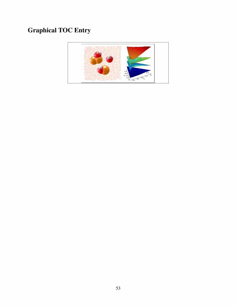
Graphical TOC Entry

53