Differentially Private Data Publishing for ArbitrarilyPartitioned Data

Rong Wanga, Benjamin C. M. Fungb, Yan Zhua, Qiang Penga

aSchool of Information Science and Technology, Southwest Jiaotong University, Chengdu610031, Sichuan, China

bSchool of Information Studies, McGill University, Montreal, QC, Canada, H3A 1X1

Abstract

Many models have been proposed to preserve data privacy for different data

publishing scenarios. Among these models, ε-differential privacy is receiving in-

creasing attention because it does not make assumptions about adversaries’ prior

knowledge and can provide a rigorous privacy guarantee. Although there are

numerous proposed approaches using ε-differential privacy to publish central-

ized data of a single-party, differentially private data publishing for distributed

data among multiple parties has not been studied extensively. The challenge in

releasing distributed data is how to protect privacy and integrity during collab-

orative data integration and anonymization. In this paper, we present the first

differentially private solution to anonymize data from two parties with arbitrar-

ily partitioned data in a semi-honest model. We aim at satisfying two privacy

requirements: (1) the collaborative anonymization should satisfy differential

privacy; (2) one party cannot learn extra information about the other party’s

data except for the final result and the information that can be inferred from

the result. To meet these privacy requirements, we propose a distributed differ-

entially private anonymization algorithm and guarantee that each step of the

algorithm satisfies the definition of secure two-party computation. In addition

to the security and cost analyses, we demonstrate the utility of our algorithm

Email addresses: wangrong.kiko@qq.com (Rong Wang), ben.fung@mcgill.ca (BenjaminC. M. Fung), yzhu@swjtu.edu.cn (Yan Zhu), qpeng@swjtu.edu.cn (Qiang Peng)

The first author conducted the research during a visit at McGill University.

Preprint submitted to Information Sciences

in classification analysis.

Keywords: data publishing, ε-differential privacy, arbitrary partitioning,

secure two-party computation, classification analysis

1. Introduction

With the development of cloud computing, data are being collected and con-

tributed by different entities, such as shopping records by chain stores, financial

data by bank branches, and census profiles by government agencies. To enable

better data analysis, distributed data are often integrated before further process-

ing. However, involving untrusted collaborators in data integration could pose

a threat to the privacy of data owners. Another threat to data privacy comes

from data publishing. Data owners sometimes intend to release their data to the

public for various purposes, including service improvement, public competition,

and academic research. For example, Netflix, an online video streaming service,

opened its previous rating data for research on movie recommendations [1].

Consider a scenario of data publishing as follows. A blood collection organi-

zation and a hospital have some information about the same individuals. They

hope to release their integrated data to a third-party for classification analysis,

such as predicting the health status of voluntary blood donors. Considering

privacy and security concerns, they do not want to violate the privacy of indi-

viduals from whom the integrated data are obtained when releasing data to the

third-party. Additionally, both parties are reluctant to share other information

with each other during their collaboration except for the necessary information

required by data integration. In the era of big data, such a scenario has become

more and more common. Thus, there is a strong motivation to develop coop-

erative anonymization methods on distributed data for privacy-preserving data

publishing.

Some approaches have been proposed to publish distributed data while pro-

tecting privacy. Jurczyk et al. [2] and Goryczka et al. [3] addressed the prob-

lem of releasing horizontally partitioned data. Jiang et al. [4, 5] generated

2

an anonymous version of vertically partitioned data without disclosing privacy.

Kohlmayer et al. [6] focused on anonymization of data that could be distributed

horizontally or vertically. Unfortunately, these works had one fundamental lim-

itation. They adopted the k-anonymity principle [7, 8] or its extensions [9, 10]

that make certain assumptions about adversaries’ prior knowledge as the un-

derlying privacy model, and they cannot provide adequate protection if the

adversaries get more information beyond these assumptions [11]. Compared to

the family of k-anonymity, ε-differential privacy [12, 13] is independent of any

adversary’s prior knowledge and can provide a more rigorous privacy guarantee.

There are numerous differentially private approaches [14, 15, 16, 17, 18, 19] to

centralized data publishing, but a very limited number of works have focused on

distributed data, especially for the scenario of arbitrarily partitioned data. In

this paper, we cover the gap with a differentially private solution to the problem

of anonymizing arbitrarily partitioned data between two parties.

Unlike horizontally and vertically partitioned data, there is no constraint on

how raw data are divided between different parties in the scenario of arbitrary

partitioning. Consider a data table of n rows and d columns that is arbitrarily

partitioned between two parties, P1 and P2. That is, for each row ri (1 ≤ i ≤ n)

of the data table, P1 holds a subset of p attributes (denoted by r1i ), and P2 holds

a subset of q attributes (denoted by r2i ), such that p + q = d (0 < q < d, 0 <

q < d), r1i ∪ r2

i = ri, and r1i ∩ r2

i = ∅. For example, values of the attributes Job

and Age in Table 1 are arbitrarily partitioned between two parties.

In this paper, we propose a differentially private algorithm to integrate two

arbitrarily partitioned data fragments into a data table while transforming the

data table into an anonymous version for classification analysis. Our work is

inspired by [14], which uses the top-down specialization (TDS) technique [20]

to anonymize centralized data in a differentially private manner. We extend

our research scope from centralized data to distributed data with an arbitrary

partitioning form. We adopt the semi-honest model, in which parties abide by

defined protocols but may try to learn extra information from their received

messages. Note that the anonymization of arbitrarily partitioned data among

3

Table 1. Data fragment arbitrarily partitioned between two parties (The first column is solely

for the purpose of illustration. For the attributes Job and Age, the underlined values and the

italicized values are held by P1 and P2, respectively. Both parties hold the Class attribute.)

No. Job Age Class

1 Teacher 35 Y

2 Clerk 25 N

3 Doctor 36 Y

4 Teacher 26 N

5 Clerk 25 N

6 Teacher 29 Y

7 Cook 38 Y

8 Clerk 23 N

9 Doctor 38 Y

10 Cook 37 Y

three or more parties will be studied in our future work. The contributions of

this paper are summarized as follows:

• We formally define the problem of differentially private data publishing

for arbitrarily partitioned data between two parties. To the best of our

knowledge, this paper is the first work that tackles this problem and ad-

dresses the challenge of securely integrating statistical information from

both horizontal and vertical dimensions.

• We propose a distributed algorithm for generating anonymous data from

two arbitrarily partitioned parties. To guarantee privacy, the anonymiza-

tion process meets both the definitions of differential privacy and secure

two-party computation; thus, during the execution of the algorithm, nei-

ther party can learn additional information on the other party’s data be-

yond what can be inferred from the final result.

• We evaluate the utility of our distributed algorithm in classification tasks.

4

Experimental results show that the algorithm can provide anonymous data

of good quality for classification analysis when compared to two single-

party algorithms, i.e., DiffGen [14] and DiffP-C4.5 [21].

The rest of the paper is organized as follows. Preliminaries including the

problem statement are presented in Section 2. The proposed algorithm is de-

scribed in Section 3 and analyzed in Section 4. Experimental results are pre-

sented in Section 5, and the related work is addressed in Section 6. Section 7

concludes the paper.

2. Preliminaries

We review ε-differential privacy and the secure protocols used in our algo-

rithm. Then we formally define the problem of differentially private data pub-

lishing for arbitrarily partitioned data between two parties. Table 2 provides

some notations used in this paper.

Table 2. List of notations

Notations Explanation Notations Explanation

P1, P2 party/data owner ε privacy budget

U universe r record

D raw dataset n number of records

D neighbor dataset d number of attributes

D′ anonymous dataset dnum number of numerical attributes

D1 data fragment held by P1 h number of specializations

D2 data fragment held by P2 l number of digits after a decimal point

M mechanism f , u function

R random number ∆f , ∆u global sensitivity

R1 random number held by P1 cls class value

R2 random number held by P2 v, c attribute value

2.1. Differential privacy

Let U represent a finite data universe, and let r represent a data record with

d attributes. A dataset D consists of n records sampled from U. Two datasets

5

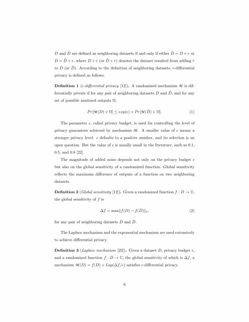
D and D are defined as neighboring datasets if and only if either D = D+ r or

D = D+ r, where D+ r (or D+ r) denotes the dataset resulted from adding r

to D (or D). According to the definition of neighboring datasets, ε-differential

privacy is defined as follows.

Definition 1 (ε-differential privacy [12]). A randomized mechanism M is dif-

ferentially private if for any pair of neighboring datasets D and D, and for any

set of possible sanitized outputs Ω,

Pr[M (D) ∈ Ω] ≤ exp(ε)× Pr[M (D) ∈ Ω]. (1)

The parameter ε, called privacy budget, is used for controlling the level of

privacy guarantees achieved by mechanism M . A smaller value of ε means a

stronger privacy level. ε defaults to a positive number, and its selection is an

open question. But the value of ε is usually small in the literature, such as 0.1,

0.5, and 0.8 [22].

The magnitude of added noise depends not only on the privacy budget ε

but also on the global sensitivity of a randomized function. Global sensitivity

reflects the maximum difference of outputs of a function on two neighboring

datasets.

Definition 2 (Global sensitivity [12]). Given a randomized function f : D → U,

the global sensitivity of f is

∆f = max‖f(D)− f(D)‖1, (2)

for any pair of neighboring datasets D and D.

The Laplace mechanism and the exponential mechanism are used extensively

to achieve differential privacy.

Definition 3 (Laplace mechanism [23]). Given a dataset D, privacy budget ε,

and a randomized function f : D → U, the global sensitivity of which is ∆f , a

mechanism M (D) = f(D) + Lap(∆f/ε) satisfies ε-differential privacy.

6

Definition 4 (Exponential mechanism [24]). Given a dataset D, output range

T , privacy budget ε, and a utility function u : (D,T )→ U, a mechanism M that

selects an output t ∈ T with probability proportional to exp( εu(D,t)2∆u ) satisfies

ε-differential privacy.

There are two important properties of differential privacy. They play a vital

role in judging whether a mechanism satisfies differential privacy.

Property 1 (Sequential composition [25]). Let M = M1,M2, · · · ,Mm be a

set of privacy mechanisms. If each Mi provides εi-differential privacy and M is

sequentially performed on a dataset, M will provide (∑mi εi)-differential privacy.

The sequential composition suggests that the privacy budget and noise ac-

cumulate linearly when a series of differentially private mechanisms is applied

to the same dataset.

Property 2 (Parallel composition [25]). Let M = M1,M2, · · · ,Mm be a set

of privacy mechanisms. If each Mi provides εi-differential privacy on a disjointed

subset of a dataset, M will provide (maxε1, ε2, · · · , εm)-differential privacy.

The parallel composition suggests that the degree of privacy protection de-

pends on the maximum value of εi when a series of differentially private mech-

anisms is applied to different subsets of a dataset.

2.2. Secure protocols

Secure comparison protocol (SCP) [26]. This is a secure protocol for Yao’s

millionaires’ problem [27], in which two integers are compared securely without

revealing their exact values.

Random value protocol (RVP) [28]. Assume that P1 holds a number R1 ∈

ZN , and P2 holds a number R2 ∈ ZN . This protocol allows the two parties to

collaboratively select a random number R ∈ ZQ such that R = (R1 + R2) mod

N ∈ [0, Q− 1], where ZN (or ZQ) is a set of non-negative integers less than N

(or Q), Q ∈ ZN is not known by either party but is shared between them, and

N is the modulus associated with the cryptosystem used in the protocol.

7

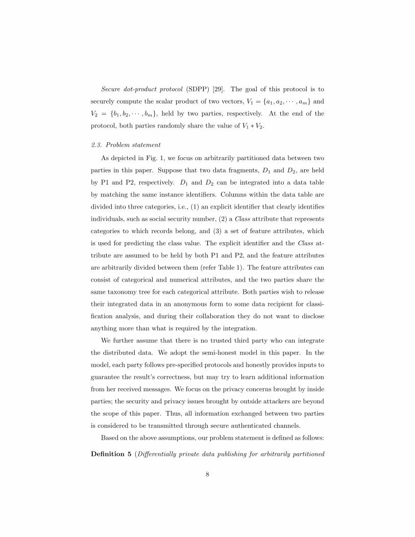
Secure dot-product protocol (SDPP) [29]. The goal of this protocol is to

securely compute the scalar product of two vectors, V1 = a1, a2, · · · , am and

V2 = b1, b2, · · · , bm, held by two parties, respectively. At the end of the

protocol, both parties randomly share the value of V1 ∗ V2.

2.3. Problem statement

As depicted in Fig. 1, we focus on arbitrarily partitioned data between two

parties in this paper. Suppose that two data fragments, D1 and D2, are held

by P1 and P2, respectively. D1 and D2 can be integrated into a data table

by matching the same instance identifiers. Columns within the data table are

divided into three categories, i.e., (1) an explicit identifier that clearly identifies

individuals, such as social security number, (2) a Class attribute that represents

categories to which records belong, and (3) a set of feature attributes, which

is used for predicting the class value. The explicit identifier and the Class at-

tribute are assumed to be held by both P1 and P2, and the feature attributes

are arbitrarily divided between them (refer Table 1). The feature attributes can

consist of categorical and numerical attributes, and the two parties share the

same taxonomy tree for each categorical attribute. Both parties wish to release

their integrated data in an anonymous form to some data recipient for classi-

fication analysis, and during their collaboration they do not want to disclose

anything more than what is required by the integration.

We further assume that there is no trusted third party who can integrate

the distributed data. We adopt the semi-honest model in this paper. In the

model, each party follows pre-specified protocols and honestly provides inputs to

guarantee the result’s correctness, but may try to learn additional information

from her received messages. We focus on the privacy concerns brought by inside

parties; the security and privacy issues brought by outside attackers are beyond

the scope of this paper. Thus, all information exchanged between two parties

is considered to be transmitted through secure authenticated channels.

Based on the above assumptions, our problem statement is defined as follows:

Definition 5 (Differentially private data publishing for arbitrarily partitioned

8

Fig. 1. Illustration of our research idea (Two parties, P1 and P2, have collected some infor-

mation from the same individuals. The information is denoted by D1 and D2, respectively.

Our research aims to integrate D1 and D2 into a data table and simultaneously transform

the data table into an anonymous version, denoted by D′. Considering privacy and security

concerns, we guarantee that our proposed algorithm satisfies ε-differential privacy and secure

two-party computation. D′ will be released to the public/third-party for data analysis.)

data between two parties). Given a data fragment D1 held by P1, another

data fragment D2 held by P2, and privacy budget ε, D1 and D2 can be in-

tegrated into a data table with n records and d feature attributes. For each row

ri (1 ≤ i ≤ n) of the data table, P1 holds a subset of p attributes (denoted by

r1i ), and P2 holds a subset of q attributes (denoted by r2

i ), such that p+ q = d

(0 < p < d, 0 < q < d), r1i ∪r2

i = ri and r1i ∩r2

i = ∅. The problem of differentially

private data publishing for arbitrarily partitioned data is to generate an inte-

grated anonymous version of D1 and D2 such that the generation algorithm (1)

satisfies ε-differential privacy and (2) follows the definition of secure two-party

computation in the semi-honest model.

3. Proposed algorithm

In this section, we first present an overview of our differentially private al-

gorithm for anonymizing arbitrarily partitioned data between two parties. We

then elaborate key steps of the algorithm.

9

3.1. Overview

Our distributed algorithm is modified significantly based on the top-down

specialization (TDS) technique [20]. As stated in [20], the specialization starts

with the most general state and goes down iteratively by replacing some values

with more specific values until reaching the predefined number of specializations.

A specialization, denoted by v → Children(v), replaces a parent value v with

its directly connected child values Children(v) according to the corresponding

taxonomy tree. For instance, in Fig. 3, Children(ANY JOB) = Professional,

Worker, and Children([1, 99)) = [1, 26), [26, 99). We also refer the parent

value that can be replaced by its directly connected child values to as “cut” in

the following.

Example 1. Fig. 2 shows a process of the TDS technique on Table 1 (data of

Table 1 is now treated as centralized data). At first, each value is generalized

to the topmost value of its corresponding taxonomy tree presented in Fig. 3,

and the initial ∪Cut is ANY JOB, [1, 99). If the ANY JOB cut is selected to

split downwards, the root of the partition tree in Fig. 2 will have two new child

nodes because of ANY JOB → Professional, Worker, and the current ∪Cut

will be updated to Professional, Worker, [1, 99), each element of which can

continue to be selected and split.

Fig. 2. Example of a partition tree

The differentially private TDS on distributed data is similar to that on cen-

tralized data. The difference is that for distributed data, the statistical informa-

10

Fig. 3. Taxonomy trees of the attributes Job and Age

tion required by the TDS should be integrated securely from different parties.

We present our Arbitrarily Distributed Differentially Private anonymization al-

gorithm (ArbDistDP) as shown in Algorithm 1. Two parties can run ArbDistDP

separately; however, Lines 4, 6, 7, 11, and 12 of ArbDistDP must be executed

collaboratively (while other lines can be done by a single party). Each of the

two parties maintains her own ∪Cut during the execution of ArbDistDP and

obtains the final integrated anonymous data same as that obtained by the other

party.

ArbDistDP consists of two phases, i.e., generalizing raw data in a top-down

manner, and adding noise to the generalized result. We adopt the uniform

allocation rule to allocate the privacy budget ε for each phase. Namely, one half

of ε is allocated for the first phase while the other half is for the second phase.

Besides, in the first phase each differentially private step consumes the same

amount of privacy budget, denoted by ε′. More specifically, an initial split value

is selected for each of dnum numerical attributes in Line 4, Line 7 is executed

h times, and Line 11 is executed at most h times; thus, the privacy budget ε′

equal to ε2(dnum+2h) is allocated for Lines 4, 7, and 11, respectively.

To ensure that ArbDistDP meets the security requirements of ε-differential

privacy and secure two-party computation, the key is to make each specializa-

tion differentially private and secure. The key steps of ArbDistDP include (1)

selection of split values, (2) calculation of utility scores, (3) selection of cuts,

and (4) adding noise. Although step (1) is presented before steps (2) and (3)

in ArbDistDP, steps (2) and (3) are described before step (1) in the following

11

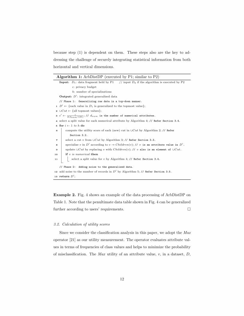
because step (1) is dependent on them. These steps also are the key to ad-

dressing the challenge of securely integrating statistical information from both

horizontal and vertical dimensions.

Algorithm 1: ArbDistDP (executed by P1; similar to P2)

Input: D1: data fragment held by P1 // input D2 if the algorithm is executed by P2

ε: privacy budget

h: number of specializations

Output: D′: integrated generalized data

// Phase 1: Generalizing raw data in a top-down manner.

1 D′ ← each value in D1 is generalized to the topmost value;

2 ∪Cut← all topmost values;

3 ε′ ← ε2(dnum+2h)

; // dnum is the number of numerical attributes.

4 select a split value for each numerical attribute by Algorithm 4; // Refer Section 3.4.

5 for i← 1 to h do

6 compute the utility score of each (new) cut in ∪Cut by Algorithm 2; // Refer

Section 3.2.

7 select a cut v from ∪Cut by Algorithm 3; // Refer Section 3.3.

8 specialize v in D′ according to v → Children(v); // v is an attribute value in D′.

9 update ∪Cut by replacing v with Children(v); // v also is an element of ∪Cut.

10 if v is numerical then

11 select a split value for v by Algorithm 4; // Refer Section 3.4.

// Phase 2: Adding noise to the generalized data.

12 add noise to the number of records in D′ by Algorithm 5; // Refer Section 3.5.

13 return D′;

Example 2. Fig. 4 shows an example of the data processing of ArbDistDP on

Table 1. Note that the penultimate data table shown in Fig. 4 can be generalized

further according to users’ requirements.

3.2. Calculation of utility scores

Since we consider the classification analysis in this paper, we adopt the Max

operator [21] as our utility measurement. The operator evaluates attribute val-

ues in terms of frequencies of class values and helps to minimize the probability

of misclassification. The Max utility of an attribute value, v, in a dataset, D,

12

Fig. 4. Data processing of ArbDistDP on one fragment of Table 1

13

is defined as follows:

Max(D, v) =∑

c∈Children(v)

max(|Dclsc |), (3)

where Children(v) is a set of directly connected child values of v, and |Dclsc | is

the number of records in D with generalized value c and class value cls. The

global sensitivity of Max(D, v) is 1 because the value of Max(D, v) varies at

most by 1 no matter whether adding or removing any single record.

Example 3. The initial ∪Cut of Table 1 is ANY JOB, [1, 99). According to

Equation (3), the utility score of ANY JOB is 7, where 7 = |DYProfessional| +

|DNWorker| = 4 + 3, and the utility score of [1, 99) is 9, where 9 = |DY

[1,26)| +

|DN[26,99)| = 3 + 6.

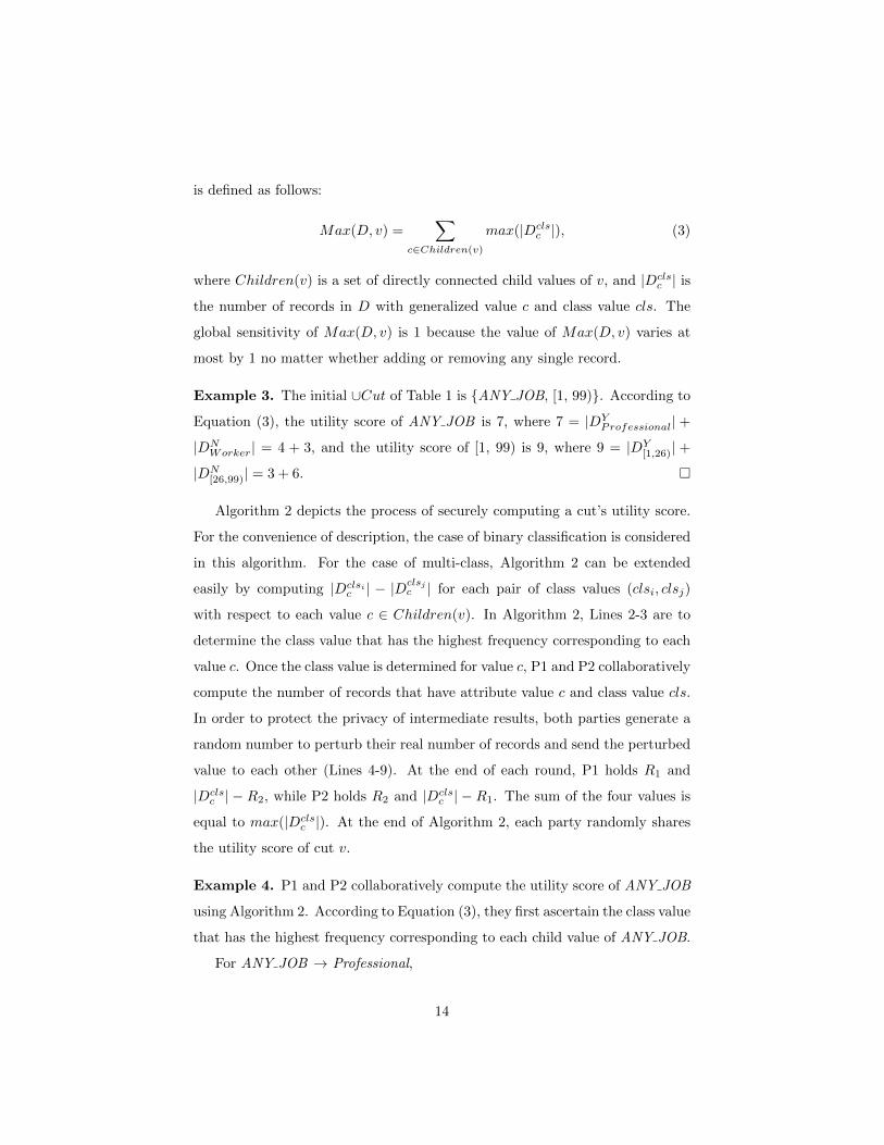
Algorithm 2 depicts the process of securely computing a cut’s utility score.

For the convenience of description, the case of binary classification is considered

in this algorithm. For the case of multi-class, Algorithm 2 can be extended

easily by computing |Dclsic | − |Dclsj

c | for each pair of class values (clsi, clsj)

with respect to each value c ∈ Children(v). In Algorithm 2, Lines 2-3 are to

determine the class value that has the highest frequency corresponding to each

value c. Once the class value is determined for value c, P1 and P2 collaboratively

compute the number of records that have attribute value c and class value cls.

In order to protect the privacy of intermediate results, both parties generate a

random number to perturb their real number of records and send the perturbed

value to each other (Lines 4-9). At the end of each round, P1 holds R1 and

|Dclsc | − R2, while P2 holds R2 and |Dcls

c | − R1. The sum of the four values is

equal to max(|Dclsc |). At the end of Algorithm 2, each party randomly shares

the utility score of cut v.

Example 4. P1 and P2 collaboratively compute the utility score of ANY JOB

using Algorithm 2. According to Equation (3), they first ascertain the class value

that has the highest frequency corresponding to each child value of ANY JOB.

For ANY JOB → Professional,

14

Algorithm 2: Securely computing the utility score of a cutInput: v: cut

Output: P1 holds one part of v’s utility score, and P2 holds the other part.

1 for ∀c ∈ Children(v) do

2 P1 calculates d1 ← |DYc | − |DNc |, and P2 calculates d2 ← |DNc | − |D

Yc |; // The

symbols Y and N denote the class values.

3 P1 and P2 run SCP to compare d1 and d2;

4 P1 generates a random number R1, and P2 generates a random number R2;

5 if d1 > d2 then

6 P1 calculates t1 ← |DYc | − R1, and P2 calculates t2 ← |DYc | − R2;

7 else

8 P1 calculates t1 ← |DNc | − R1, and P2 calculates t2 ← |DNc | − R2;

9 P1 sends t1 to P2, and P2 sends t2 to P1;

10 P1/P2 calculates the sum of all random numbers she generated and all values she

received; // The sum is part of v’s utility score held by P1/P2.

P1: |DYProfessional| = 1, |DN

Professional| = 1

d1 = |DYProfessional| − |DN

Professional| = 1− 1 = 0

P2: |DNProfessional| = 0, |DY

Professional| = 3

d2 = |DNProfessional| − |DY

Professional| = 0− 3 = −3

As d1 > d2, the value Professional corresponds to the class value Y with the

higher frequency compared to the class value N. P1 and P2 separately generate

a random number to perturb their real number of records with attribute value

Professional and class value Y.

P1: R1 = 1, |DYProfessional| −R1 = 1− 1 = 0

P2: R2 = 2, |DYProfessional| −R2 = 3− 2 = 1

P1 sends the perturbed value 0 to P2, and P2 sends the perturbed value 1 to

P1. P1 calculates the sum of the random number she generated and the value

she received, which is 1+1 = 2. Similarly, P2 gets the sum 2, which is 2+0 = 2.

Thus, |DYProfessional| = 4, of which P1 and P2 each hold a half separately.

After the similar calculation of ANY JOB →Worker, both parties randomly

share the entire utility score of ANY JOB.

15

3.3. Selection of cuts

After obtaining each cut’s utility score, P1 and P2 collaboratively select a

cut from the current ∪Cut. The exponential mechanism is adopted in this step

because it is designed for discrete alternatives. According to Definition 4, the

exponential mechanism selects a candidate with the probability proportional

to its utility score. We extend the distributed exponential mechanism Dist-

Exp proposed in [30]. The general idea of DistExp is to divide the range [0,∑i exp(

εui2∆u )] into multiple segments, each corresponding to a cut and having

a sub-interval of length equal to exp( εui2∆u ), then to uniformly select a random

number from the range [0,∑i exp(

εui2∆u )]. The segment in which the random

number falls corresponds to the winner cut. For example, in Fig. 5 the proba-

bility of selecting a random value from Segment 1, Segment 2, Segment 3, and

Segment 4 of the range [0, 1] is 20%, 30%, 10%, and 40%, respectively.

Fig. 5. Example of a segmentation of the range [0, 1]

The challenge facing us is the randomness share of the utility score of each

cut. To tackle this problem, we leverage one property of the exponential func-

tion, i.e., exp( εu2∆u ) = exp( ε(u1+u2)

2∆u ) = exp( εu1

2∆u ) × exp( εu2

2∆u ), where u is the

entire utility score of a cut, u1 and u2 are held by P1 and P2 respectively, and

u1 + u2 = u. Then we let P1 and P2 use SDPP to compute the product of

exp( εu1

2∆u ) and exp( εu2

2∆u ). In fact, this calculation is treated as converting the

values of exp( εu1

2∆u ) and exp( εu2

2∆u ) into two vectors and using SDPP to compute

the inner product of the two vectors.

The two parties run RVP to collaboratively select a random number from

the range [0,∑i exp(

εui2∆u )]. The RVP works only for integers, but exp( εui2∆u )

may be a floating-point number. In this case, before computing the product

16

we scale floating-point numbers by taking their floor values of exp( εui2∆u ) × 10l,

where l is the number of the considered digits after the decimal point, which

can be predefined by the parties. Such a scaling is a common method of dealing

with floating-point numbers in cryptography [31]. We present the process of

securely selecting a cut in Algorithm 3.

Algorithm 3: Securely selecting a cutInput: current cuts ∪Cut and their utility scores

Output: winner cut

1 for i← 1 to | ∪ Cut| do

2 P1 calculates si1 ← exp(εui12∆u ), and P2 calculates si2 ← exp(

εui22∆u );

3 P1 and P2 run SDPP to compute the product of si1 and si2; one part of the product

(denoted by ti1) is held by P1, while the other part (denoted by ti2) is held by P2;

4 P1 calculates T1 ←∑ti1, and P2 calculates T2 ←

∑ti2;

5 P1 and P2 run RVP to securely select a random number R from the range [0, T1 + T2]; P1

gets R1, and P2 gets R2, where R1 + R2 = R;

6 for i← 1 to | ∪ Cut| do

7 P1 calculates C1 ← ti1 − R1, and P2 calculates C2 ← R2 − ti2;

8 P1 and P2 run SCP to compare C1 and C2;

9 if C1 > C2 then

// This case means ti1 + ti2 > R.

10 return the ith cut of ∪Cut;

Example 5. Continued from Example 3. Consider the ANY JOB cut, the

utility score of which is equal to 7. Suppose that P1 holds one part of the utility

score, u1 = 3, and P2 holds the other part, u2 = 4. Set ε = 0.5 and l = 1.

P1: sANY JOB1 = exp( 0.5×3

2×1 ) ≈ 2.1170

P2: sANY JOB2 = exp( 0.5×4

2×1 ) ≈ 2.7183

After scaling, P1 ends up with the value 21, and P2 ends up with the value

27. The product of 21 and 27 is equal to 567, and suppose that P1 holds a value

186 while P2 holds a value 381, where 186 + 381 = 567.

For the [1, 99) cut, the utility score of which is equal to 9, suppose that P1

holds one part of the utility score, u1 = 7, and P2 holds the other part, u2 = 2.

P1: s[1,99)1 = exp( 0.5×7

2×1 ) ≈ 5.7546

P1: s[1,99)2 = exp( 0.5×2

2×1 ) ≈ 1.6487

17

P1 ends up with the value 57 and P2 ends up with the value 16 after scaling.

The product of 57 and 16 is equal to 912, and suppose that P1 holds a value

405, while P2 holds a value 507, where 405 + 507 = 912.

The parties collaboratively select a random number from the range [0, 1479]

using the RVP, where 1479 = 567 + 912. Suppose that the random number

R is 263, for which P1 holds a value 95, and P2 holds a value 168. For the

first candidate ANY JOB, P1 calculates C1 = 186− 95 = 91, and P2 calculates

C2 = 168− 381 = −213. Because 91 > −213, the random number R lies in the

range [0, 567), which means that ANY JOB is selected as the winner cut.

3.4. Selection of split values

We assume that a taxonomy tree is provided for each categorical attribute,

and both parties know it as their prior knowledge. Thus, categorical cuts are

split downwards directly according to their corresponding taxonomy trees.

As mentioned in [20], there is no need to provide taxonomy trees for numeri-

cal attributes. If a numerical cut is selected to split, its corresponding taxonomy

tree can be grown dynamically by searching for a split value for the numerical

cut. A split value should not be picked randomly because the probability of

choosing the same value from a dataset not containing this value is 0. This

means that the selection on a split value for a numerical attribute is probabilis-

tic. Our selection strategy is to split the numerical domain into two sub-intervals

by each numerical value and calculate the utility scores of these sub-intervals.

After all the numerical values in the domain have been processed, Algorithm 3

is adopted to select a value as the split value according to the utility scores of

its corresponding sub-intervals.

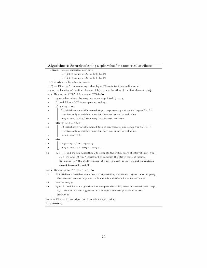
Algorithm 4 depicts the process of securely selecting a split value for a nu-

merical attribute. In Lines 1-2 of the algorithm, P1 and P2 separately sort their

values of the target numerical attribute in ascending order and generate cursors

to point to the first element of their sorted lists. In Lines 3-16, both parties

securely compare the values pointed to by cur1 and cur2. They know the result

of each secure comparison, and the party who holds the smaller number sends a

18

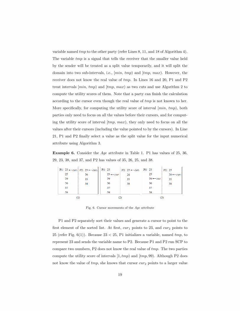
variable named tmp to the other party (refer Lines 8, 11, and 18 of Algorithm 4).

The variable tmp is a signal that tells the receiver that the smaller value held

by the sender will be treated as a split value temporarily, and it will split the

domain into two sub-intervals, i.e., [min, tmp) and [tmp, max). However, the

receiver does not know the real value of tmp. In Lines 16 and 20, P1 and P2

treat intervals [min, tmp) and [tmp, max) as two cuts and use Algorithm 2 to

compute the utility scores of them. Note that a party can finish the calculation

according to the cursor even though the real value of tmp is not known to her.

More specifically, for computing the utility score of interval [min, tmp), both

parties only need to focus on all the values before their cursors, and for comput-

ing the utility score of interval [tmp, max), they only need to focus on all the

values after their cursors (including the value pointed to by the cursors). In Line

21, P1 and P2 finally select a value as the split value for the input numerical

attribute using Algorithm 3.

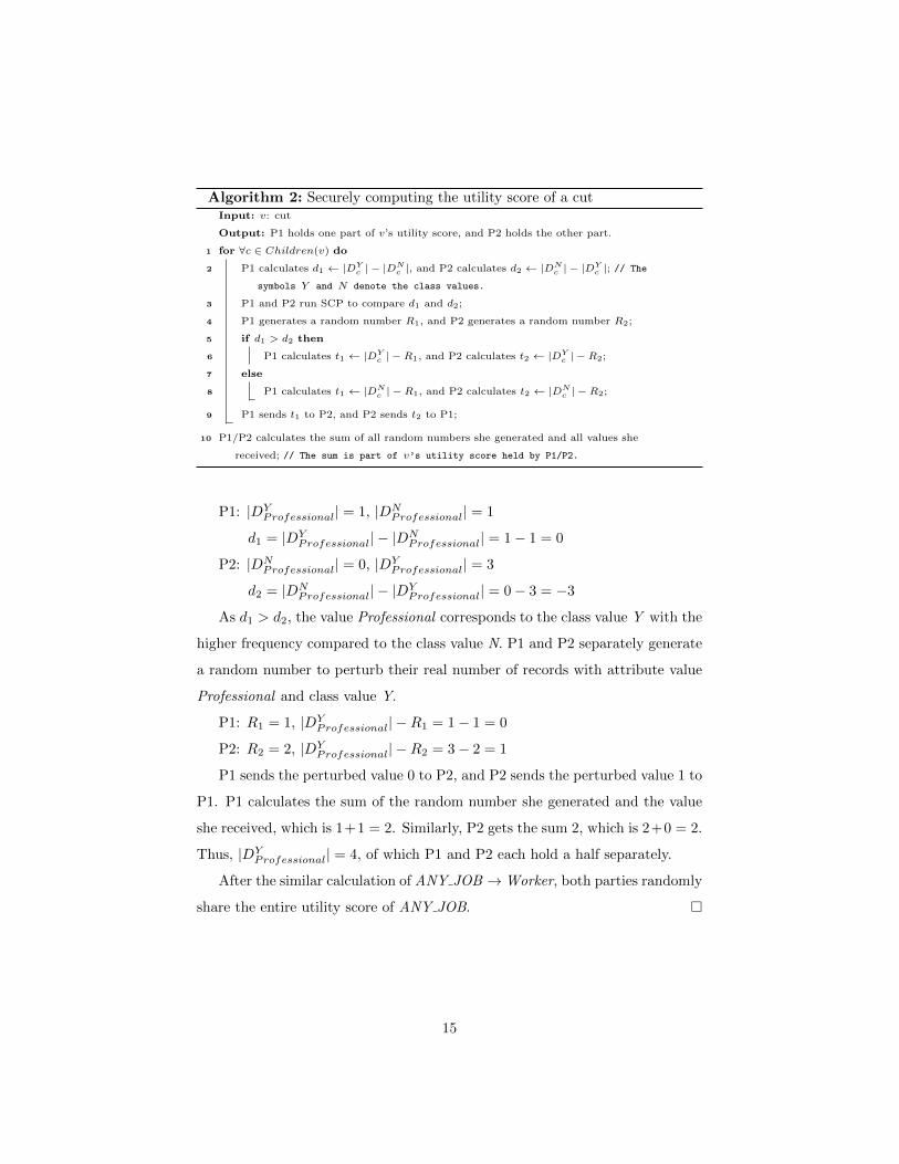
Example 6. Consider the Age attribute in Table 1. P1 has values of 25, 36,

29, 23, 38, and 37, and P2 has values of 35, 26, 25, and 38.

Fig. 6. Cursor movements of the Age attribute

P1 and P2 separately sort their values and generate a cursor to point to the

first element of the sorted list. At first, cur1 points to 23, and cur2 points to

25 (refer Fig. 6(1)). Because 23 < 25, P1 initializes a variable, named tmp, to

represent 23 and sends the variable name to P2. Because P1 and P2 run SCP to

compare two numbers, P2 does not know the real value of tmp. The two parties

compute the utility score of intervals [1, tmp) and [tmp, 99). Although P2 does

not know the value of tmp, she knows that cursor cur2 points to a larger value

19

Algorithm 4: Securely selecting a split value for a numerical attributeInput: Anum: numerical attribute

L1: list of values of Anum held by P1

L2: list of values of Anum held by P2

Output: v: split value for Anum

1 L′1 ← P1 sorts L1 in ascending order, L′

2 ← P2 sorts L2 in ascending order;

2 cur1 ← location of the first element of L′1, cur2 ← location of the first element of L′

2;

3 while cur1 6= NULL && cur2 6= NULL do

4 v1 ← value pointed by cur1, v2 ← value pointed by cur2;

5 P1 and P2 run SCP to compare v1 and v2;

6 if v1 < v2 then

7 P1 initializes a variable named tmp to represent v1 and sends tmp to P2; P2

receives only a variable name but does not know its real value.

8 cur1 ← cur1 + 1; // Move cur1 to the next position.

9 else if v2 < v1 then

10 P2 initializes a variable named tmp to represent v2 and sends tmp to P1; P1

receives only a variable name but does not know its real value.

11 cur2 ← cur2 + 1;

12 else

13 tmp← v1; // or tmp← v2

14 cur1 ← cur1 + 1, cur2 ← cur2 + 1;

15 s1 ← P1 and P2 run Algorithm 2 to compute the utility score of interval [min, tmp),

s2 ← P1 and P2 run Algorithm 2 to compute the utility score of interval

[tmp,max); // The utility score of tmp is equal to s1 + s2 and is randomly

shared between P1 and P2.

16 while curi 6= NULL (i = 1or 2) do

17 Pi initializes a variable named tmp to represent vi and sends tmp to the other party;

the receiver receives only a variable name but does not know its real value.

18 curi ← curi + 1;

19 s1 ← P1 and P2 run Algorithm 2 to compute the utility score of interval [min, tmp),

s2 ← P1 and P2 run Algorithm 2 to compute the utility score of interval

[tmp,max);

20 v ← P1 and P2 use Algorithm 3 to select a split value;

21 return v;

20

than tmp. Thus, P2 concludes that interval [1, tmp) includes values before cur2,

and the interval [tmp, 99) includes the values after cur2 (including the value

pointed to by cur2). After collaboratively getting utility scores of intervals [1,

tmp) and [tmp, 99), P1 moves cur1 to the next position (refer Fig. 6(2)).

As shown in Fig. 6(2), both cur1 and cur2 point to 25. Because 25 = 25,

P1 and P2 cooperatively compute the utility score of intervals [1, tmp) and

[tmp, 99), where the value of tmp is equal to 25. After getting utility scores

of intervals [1, 25) and [25, 99), both parties move their cursors to the next

position respectively (refer Fig. 6(3)).

The parties continue the above process until both cur1 and cur2 reach the

end of the sorted lists. P1 and P2 finally select a split value using Algorithm 3

according to the sum of the utility scores of the corresponding sub-intervals.

3.5. Adding noise

After the raw data are generalized to a specific level, it is necessary to add

noise to them. This is because for a different dataset, the number of records

in each leaf node of the partition tree may be different and publishing the real

number could violate differential privacy. We use the terms “leaf node” and

“equivalence group” interchangeably in the following. This difference can be

offset easily by adding noise to the number of records in each equivalence group.

We adopt the secure mechanism used in [30] to add noise. In this mechanism,

both parties first calculate the number of records in each group and add noise

to the number using the Laplace mechanism. Algorithm 5 depicts the secure

mechanism. Next, we elaborate key steps of Algorithm 5.

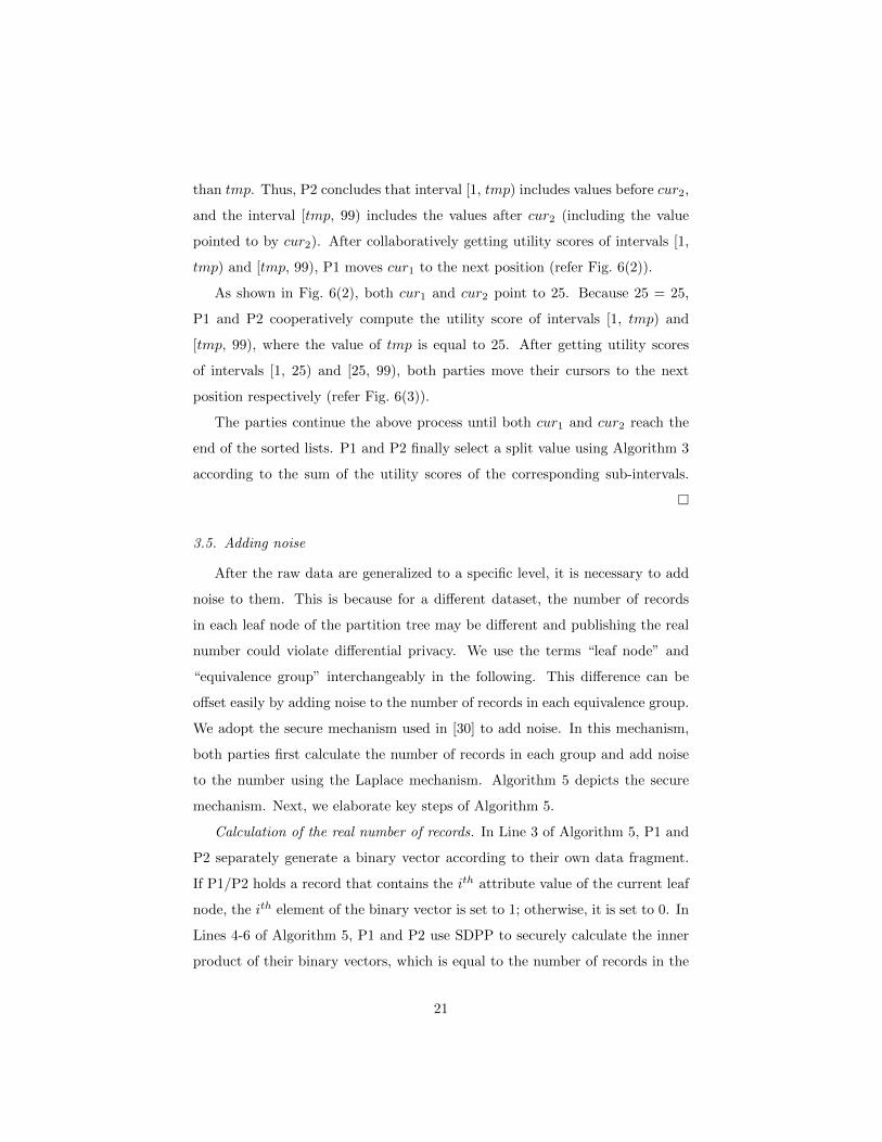
Calculation of the real number of records. In Line 3 of Algorithm 5, P1 and

P2 separately generate a binary vector according to their own data fragment.

If P1/P2 holds a record that contains the ith attribute value of the current leaf

node, the ith element of the binary vector is set to 1; otherwise, it is set to 0. In

Lines 4-6 of Algorithm 5, P1 and P2 use SDPP to securely calculate the inner

product of their binary vectors, which is equal to the number of records in the

21

Algorithm 5: Generating the final integrated data

Input: partition tree maintained by P1/P2 // Note that the tree held by P1 is the

same as the tree held by P2.

Output: D′: integrated anonymous data

1 P1 generates a cryptographic key pair (PK, SK) of a homomorphic encryption scheme

and sends PK to P2.

2 for ∀node ∈ leaf nodes of the partition tree do

// compute the number of records in node

3 P1 generates a binary vector V1 ← (a1, a2, · · · , an), where ai = 1(1 ≤ i ≤ n) P1 has

the records that contains the ith attribute value of node; otherwise, ai ← 0; P2

generates a binary vector V2 ← (b1, b2, · · · , bn), where bi = 1(1 ≤ i ≤ n) if P2 has

the records that contains the ith attribute value of node; otherwise, bi ← 0;

4 P1 encrypts V1 with PK and sends the encrypted vector (e(a1), e(a2), · · · , e(an)) to

P2;

5 P2 generates a random number C2, encrypts it with PK, and computes

P = e(R) ·∏ni=1 yi, where yi = e(ai) if bi = 1, and yi = 1 if bi = 0; P2 sends P to

P1;

6 P1 uses SK to decrypt the value received from P2 and gets the result, C1;

// add noise to the number of records

7 P1 randomly samples two variables, t1 and t2, from Gaussian distribution

N (0,√

1/ε) and computes X1 ← C1 + t21 − t22, and then sends X1 to P2; P2

randomly samples two variables, t3 and t4, from Gaussian distribution N (0,√

1/ε)

and computes X2 ← C2 + t23 − t24, and then sends X2 to P1;

8 X ← X1 +X2;

9 D′ ← D′∪ the generalized record in node, of which the noisy number of records is X;

10 return D′;

22

leaf node.

Example 7. Consider the number of records in the bottom right leaf node,

i.e., <Worker, [26, 99)>, in Fig. 2 is required. The leaf node contains records

whose job can be generalized to Worker and age can be generalized to the

range [26, 99). As detailed in Table 3, P1 generates the binary vector V1 =

0, 0, 1, 0, 1, 1, 1, 0, 1, 1 while P2 generates the binary vector V2 = 1, 1, 0, 1, 0, 0, 1, 1, 0, 1.

P1 and P2 use SDPP to securely compute the inner product of V1 and V2 such

that

V1 · V2 =

10∑i=1

Z1(i)× Z2(i) = 0 + 0 + 0 + 0 + 0 + 0 + 1 + 0 + 0 + 1 = 2

At the end of SDPP, the parties have random shares of the result V1 ·V2, which

is equal to the number of records in leaf node <Worker, [26, 99)>.

Table 3. Binary vectors generated by two parties according to leaf node <Worker, [26, 99)>

No.P1 P2

Job Age V1(i) Job Age V2(i)

1 Professional 0 [26, 99) 1

2 [1, 26) 0 Worker 1

3 [26, 99) 1 Professional 0

4 Professional 0 [26, 99) 1

5 Worker 1 [1, 26) 0

6 [26, 99) 1 Professional 0

7 Worker 1 [26, 99) 1

8 [1, 26) 0 Worker 1

9 [26, 99) 1 Professional 0

10 [26, 99) 1 Worker 1

Lemma 1. [32, 30] Given four Gaussian random variables, i.e., ti ∼ N (0, λ)

for i ∈ 1, 2, 3, 4, the random variable Lap(2λ2) is equal to t21 + t22 − t23 − t24.

Calculation of the noisy number of records. According to Lemma 1, a ran-

dom variable sampled from Lap(2λ2) is equal to the linear combination of four

23

random variables sampled from N (0, λ). As mentioned before, ε/2 is used for

obtaining the noisy number of records. It is easy to make an equation, 2λ2 = 2/ε,

and get the value of λ, which is equal to√

1/ε. Thus, to calculate the noisy

number, P1 only needs to calculate X1 ← C1 + t21− t23, where C1 is the random

share of V1 ·V2 held by P1, and t1 and t3 are sampled from Gaussian distribution

N (0,√

1/ε) by P1; similarity, P2 only needs to calculate X2 ← C2 + t22 − t24,

where C2 is the random share of V1 · V2 held by P2, and t2 and t4 are sampled

from Gaussian distribution N (0,√

1/ε) by P2. Then P1 sends X1 to P2 while

P2 sends X2 to P1 (refer Line 7 of Algorithm 5). The noisy number of records

in each leaf node, denoted by X, is calculated as follows:

X = C + Lap(2/ε)

= X1 +X2

= C1 + t21 − t23 + C2 + t22 − t24.

(4)

, where C is the real number, Lap(2/ε) is the added noise, X1 is held by P1,

and X2 is held by P2.

Example 8. Noise is added to the number of records in each leaf node of the

partition tree in Fig. 2 (refer the dotted arrows).

4. Analysis of the algorithm

We analyze the correctness, security, and complexity of ArbDistDP in this

section.

Theorem 1 (Correctness). ArbDistDP satisfies ε-differential privacy.

Proof. Instead of developing new mechanisms, we use two existing mechanisms,

i.e., the Laplace mechanism and the exponential mechanism, to design Arb-

DistDP. So, we prove Theorem 1 by proofing all differentially private operations

in the algorithm following the two mechanisms. We first prove that all sub-

algorithms used in ArbDistDP satisfy differential privacy.

24

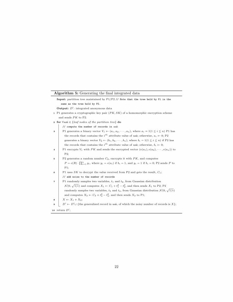
– Algorithm 2 calculates the utility score of each cut that may be selected

to split downwards. According to [24], the utility scores of candidates

required by the exponential mechanism are based on the real counts from

the raw data. Thus, Algorithm 2 does not violate differential privacy.

– Algorithm 3 selects a cut v from ∪Cut with probability proportional

to exp( εui2∆u ). Two parties separately compute part of the utility score

exp( εui2∆u ) of each cut. They then build a range [0,∑ni=1 exp(

εui2∆u )] and

partition the range into sub-intervals, each of which has a length equal to

exp( εui2∆u ). A cut is selected according to a random value that lies uni-

formly in the range [0,∑ni=1 exp(

εui2∆u )], thus the probability of choosing

any cut is equal toexp(

εui2∆u )∑n

i=1 exp(εui2∆u )

. Therefore, Algorithm 3 implements the

exponential mechanism and satisfies differential privacy.

– Lines 1-20 of Algorithm 4 also calculate the utility score of each candidate

that may be selected as a split value. Line 21 of Algorithm 4 uses the

exponential mechanism to do the selection. Thus, Algorithm 4 does not

violate differential privacy.

– Algorithm 5 uses the Laplace mechanism to output the noisy number of

records in each leaf node of the partition tree, where the noises are sampled

from Lap(2/ε). Thus, Algorithm 5 satisfies differential privacy.

Next, we prove that each step of ArbDistDP satisfies differential privacy.

– Line 4 of ArbDistDP selects an initial split value for each numerical at-

tribute using Algorithm 4. The privacy budget costed by each exponential

mechanism is ε′, so the step guarantees ε′ × dnum-differential privacy ac-

cording to the sequential composition property.

– Line 7 of ArbDistDP selects a cut to split using Algorithm 3, and the step

also satisfies ε′-differential privacy.

– Line 11 of ArbDistDP selects a split value for a new numerical cut using

Algorithm 4, which also satisfies ε′-differential privacy.

25

– Line 12 of ArbDistDP outputs the noisy count of each leaf node (equiva-

lence group) of the partition tree using Algorithm 5 and guarantees ε/2-

differential privacy.

– The rest of the lines of ArbDistDP are not affected when adding/removing

a single record to/from the raw data; thus, these steps do not violate

differential privacy.

Each non-deterministic step of ArbDistDP is differentially private, and the

total privacy budget is not greater than ε. Hence, ArbDistDP satisfies ε-

differential privacy according to the sequential composition property.

Theorem 2 (Security). ArbDistDP satisfies secure two-party computation.

Proof. The security of ArbDistDP depends on all the steps in which two par-

ties exchange information. Since Algorithms 2, 3, and 4 are sub-algorithms

of ArbDistDP, we prove the security of ArbDistDP by proving the security of

Algorithms 2, 3, and 4.

– In Algorithm 2, the steps in which two parties exchange their information

are only Lines 3 and 9. In Line 3, the SCP that securely compares two

integers has been proven to be secure [26]. In Line 9, both parties share

their values of |Dclsc | − Ri (where Ri is a random number) with each

other, rather than the real value of |Dclsc |. This step also is secure. Thus,

Algorithm 2 satisfies secure two-party computation.

– In Algorithm 3, the steps in which the two parties communicate with each

other are Lines 3, 5, and 8. The SDPP used in Line 3 and the RVP used

in Line 5 have been proven to be secure in [29] and [28], respectively. The

security of SCP in Line 8 has been mentioned above. Thus, Algorithm 3

satisfies secure two-party computation.

– In Algorithm 4, the steps in which the two parties exchange their infor-

mation are Lines 5, 8, 11, 16, 18, 20, and 21. The SCP used in Line 5

26

is secure. Note that in Lines 8, 11, and 18, P1 (or P2) sends a variable

named tmp to P2 (or P1) instead of the real value; hence, these steps

are secure without revealing real information. Lines 16 and 20 are secure

according to the security of Algorithm 2. Similarly, Line 21 also is se-

cure according to the security of Algorithm 3. Thus, Algorithm 4 satisfies

secure two-party computation.

In summary, ArbDistDP satisfies secure two-party computation because of

the composition theorem [33].

Theorem 3 (Complexity). The computation and communication complexity of

ArbDistDP are bounded by O(hnL2 + hnK2) +O(2hn) and O(hnL2 + hnK) +

O(2hne), respectively, where h is the number of specializations, n is the size

of the integrated anonymous data, L is the bit length of operands used in the

SCP, K is the security parameter of the encryption scheme used in the RCP

and SSDP, and e is the bit length of an encrypted item.

Proof. The computation and communication complexity of ArbDistDP depend

on the secure computation protocols used between two parties. The protocols

instrumented inside ArbDistDP are SCP, RVP, and SSDP.

– The computation and communication complexity of SCP proposed in [26]

are both O(L2).

– The computation and communication complexity of RVP proposed in [28]

are both O(K2).

– The computation and communication complexity of SSDP proposed in [29]

are O(K2) and O(K).

Let the maximum values of |Children(v)| and | ∪ Cut| be m1 and m2, re-

spectively. Thus, the computation complexity of Algorithms 2, 3, and 4 are

O(m1L2), O(m2K

2 + m2L2), and O(nL2 + nK2), respectively. And the com-

munication costs for Algorithms 2, 3, and 4 are O(m1d2), O(m2K+m2L

2), and

O(nL2 + nK), respectively.

27

The number of leaf nodes is 2h, and the computation and communication

complexity of adding noise to leaf nodes are O(2hn) and O(2hne), respectively.

In summary, as both parties execute h specializations, the total compu-

tation and communication costs of ArbDistDP are O(hm1L2) + O(hm2K

2 +

hm2L2) +O(hnL2 + hnK2) +O(2hn) and O(hm1L

2) +O(hm2K + hm2L2) +

O(hnL2 + hnK) + O(2hne), respectively. Because n m1 and n m2,

we limit the computation and communication complexity of ArbDistDP to

O(hnL2 + hnK2) +O(2hn) and O(hnL2 + hnK) +O(2hne), respectively.

5. Experimental evaluation

In this section, we evaluate the performance of ArbDistDP. First, we study

the effect of privacy budgets and scaling operations on the utility of the in-

tegrated anonymous data generated by ArbDistDP. Second, we compare Arb-

DistDP with two single-party anonymization algorithms. Third, we estimate

the scalability of ArbDistDP.

All experiments were performed on a PC with a 3.4 GHz @Intel core i7 CPU

and 16 GB of RAM running Windows 10 (64-bit). Each result presented below

is the average over 5 runs.

5.1. Datasets and metrics

Two publicly available datasets, i.e., Adult and Nursery, are used in our

experiments. The Adult3 dataset is a de facto benchmark for testing the per-

formance of anonymization algorithms [21, 30, 34, 35, 36, 37, 38]. It contains

45,222 census records with 8 categorical attributes, 6 numerical attributes, and

a Class attribute representing two kinds of income levels, i.e., ≤50K, and >50K.

The second dataset, Nursery4, consists of personal information of individuals

who apply for admission to a nursery school. It contains 12,960 records with

3https://archive.ics.uci.edu/ml/datasets/adult4https://archive.ics.uci.edu/ml/datasets/nursery

28

Table 4. Details of two datasets

Datasets Records Attributes

Adult45,222 14

(≤50K : 34,014 >50K : 11,208) (CA: 8 NA: 6)*

Nursery12,960 8

(not recom: 4,320 priority: 4,266 spec prior:

4,044 very recom: 328 recommend: 2)

(CA: 8)

* CA: categorical attributes NA: numerical attributes

8 categorical attributes, and a Class attribute representing five categories, in-

cluding not-recom, priority, spec-prior, very-recom, and recommend. Details of

the two datasets are presented in Table 4.

For the classification analysis, we randomly divide each dataset into two

subsets, i.e., a training dataset and a testing dataset. To construct the scenario

of arbitrarily partitioned data, we randomly select arbitrary attributes from

each of the raw records to be held by P1 and let the remaining attributes be

held by P2. We apply ArbDistDP to the training dataset to obtain a ∪Cut and

apply the ∪Cut to the testing dataset to produce a generalized testing dataset.

We then build a classifier on the generalized training dataset. The metrics for

measuring the utility of the generalized testing dataset are defined as follows:

– Classification accuracy(CA): the classification accuracy on the generalized

testing dataset;

– BA-CA: the cost of achieving a given ε-differential privacy requirement,

where BA is the abbreviated form of baseline accuracy that is the classifi-

cation accuracy measured on the raw dataset without any anonymization;

– CA-LA: the benefit of an algorithm over the random guessing, where LA

is the abbreviated form of lower-bound accuracy that is the classification

accuracy on the raw dataset with all attributes (except for the Class at-

tribute) removed.

29

Note that CA is in the range of 0 to 1. The larger the value of CA is, the

higher the utility of the generalized dataset is. The decision tree with default

parameters in RapidMiner Studio was adopted for the classification model. The

number of specializations, h, was set to 10 for ArbDistDP.

5.2. Experimental results

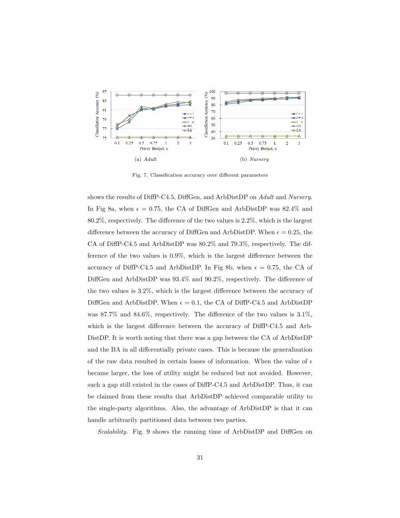
Data utility over different parameters. Fig. 7 shows the classification accu-

racy of ArbDistDP on Adult and Nursery, where the privacy budget 0.1 ≤ ε ≤ 3,

and the scaling parameter 2 ≤ l ≤ 6. It can be seen from the figure that the

CA of all differentially private cases increased as ε increased. This occurred

because a higher ε resulted in better attribute partitioning, and it reduced the

magnitude of noise added to the number of records in each equivalence group.

More specifically, in Fig. 7a BA and LA were 84.2% and 75.2%, respectively. For

ε = 0.1 and l = 2, BA-CA was 7.2% whereas CA-LA was 1.8%. As ε increased

to 3, CA increased to around 82.8%, the cost decreased to about 1.4%, and the

benefit increased to about 7.6%. In Fig. 7b, BA and LA were 97.3% and 33.3%,

respectively. For ε = 0.1 and l = 2, BA-CA was 15.8% whereas CA-LA was

48.2%. As ε increased to 3, CA increased to around 91.5%, the cost decreased

to about 5.8%, and the benefit increased to about 58.2%. There was another

trend of the CA affected by scaling parameter l. The largest span of the CA in

Fig. 7a was from 78.5% to 79.8% when ε = 0.25 and l varied from 2 to 4. The

rest of CA for different values of l were close to each other if ε was fixed. Fig. 7b

shows the similar trends of the CA for Nursery, with the only difference being

in the case of the values of ε and l when getting the largest span. These results

mean that the scaling operation had limited impact on the data utility.

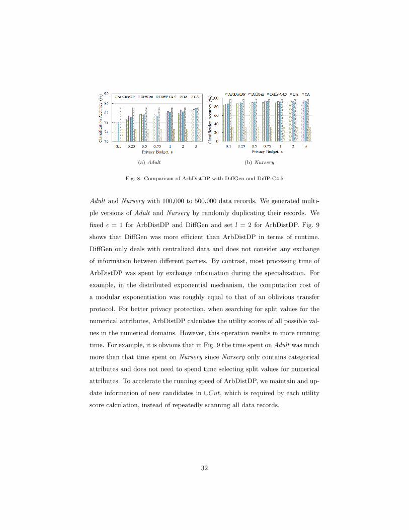
Data utility over different algorithms. We compared ArbDistDP with Dif-

fGen [14], by which our work is inspired. Both algorithms are combined with

the generalization technique with output perturbation to mask raw data, but

DiffGen only handles centralized data of a single party. We also compared Arb-

DistDP with another single-party algorithm, DiffP-C4.5 [21], which is an inter-

active algorithm for building a classifier. We set l = 2 for ArbDistDP. Fig. 8

30

(a) Adult (b) Nursery

Fig. 7. Classification accuracy over different parameters

shows the results of DiffP-C4.5, DiffGen, and ArbDistDP on Adult and Nursery.

In Fig 8a, when ε = 0.75, the CA of DiffGen and ArbDistDP was 82.4% and

80.2%, respectively. The difference of the two values is 2.2%, which is the largest

difference between the accuracy of DiffGen and ArbDistDP. When ε = 0.25, the

CA of DiffP-C4.5 and ArbDistDP was 80.2% and 79.3%, respectively. The dif-

ference of the two values is 0.9%, which is the largest difference between the

accuracy of DiffP-C4.5 and ArbDistDP. In Fig 8b, when ε = 0.75, the CA of

DiffGen and ArbDistDP was 93.4% and 90.2%, respectively. The difference of

the two values is 3.2%, which is the largest difference between the accuracy of

DiffGen and ArbDistDP. When ε = 0.1, the CA of DiffP-C4.5 and ArbDistDP

was 87.7% and 84.6%, respectively. The difference of the two values is 3.1%,

which is the largest difference between the accuracy of DiffP-C4.5 and Arb-

DistDP. It is worth noting that there was a gap between the CA of ArbDistDP

and the BA in all differentially private cases. This is because the generalization

of the raw data resulted in certain losses of information. When the value of ε

became larger, the loss of utility might be reduced but not avoided. However,

such a gap still existed in the cases of DiffP-C4.5 and ArbDistDP. Thus, it can

be claimed from these results that ArbDistDP achieved comparable utility to

the single-party algorithms. Also, the advantage of ArbDistDP is that it can

handle arbitrarily partitioned data between two parties.

Scalability. Fig. 9 shows the running time of ArbDistDP and DiffGen on

31

(a) Adult (b) Nursery

Fig. 8. Comparison of ArbDistDP with DiffGen and DiffP-C4.5

Adult and Nursery with 100,000 to 500,000 data records. We generated multi-

ple versions of Adult and Nursery by randomly duplicating their records. We

fixed ε = 1 for ArbDistDP and DiffGen and set l = 2 for ArbDistDP. Fig. 9

shows that DiffGen was more efficient than ArbDistDP in terms of runtime.

DiffGen only deals with centralized data and does not consider any exchange

of information between different parties. By contrast, most processing time of

ArbDistDP was spent by exchange information during the specialization. For

example, in the distributed exponential mechanism, the computation cost of

a modular exponentiation was roughly equal to that of an oblivious transfer

protocol. For better privacy protection, when searching for split values for the

numerical attributes, ArbDistDP calculates the utility scores of all possible val-

ues in the numerical domains. However, this operation results in more running

time. For example, it is obvious that in Fig. 9 the time spent on Adult was much

more than that time spent on Nursery since Nursery only contains categorical

attributes and does not need to spend time selecting split values for numerical

attributes. To accelerate the running speed of ArbDistDP, we maintain and up-

date information of new candidates in ∪Cut, which is required by each utility

score calculation, instead of repeatedly scanning all data records.

32

(a) Adult (b) Nursery

Fig. 9. Scalability on Adult and nursery

6. Related work

Relational data anonymization. Research on relational data anonymization

started with Samarati [7] and Sweeney [8]. They formalized a model called

k-anonymity to resist record linkage attacks by generalizing or suppressing cer-

tain identifying attributes. Many variants of the model have been proposed for

preserving data privacy further. Amiri et al. [34] proposed algorithms to gener-

ate k-anonymous β-likeness data that prevent identity and attribute disclosures

and hide the correlations between identifying attributes and sensitive attributes.

Zhu et al. [35] presented an independent l-diversity principle and its implemen-

tation to prevent corruption attacks while maintaining the utility of published

data. Wang et al. [36] used the t-closeness model [9] to protect the privacy of

multiple sensitive attributes. Agarwal et al. [37] proposed a (P , U)-sensitive

k-anonymity model for protecting sensitive records rather than protecting sen-

sitive attributes. Unfortunately, these works fail to provide rigorous privacy

guarantees because their underlying privacy models rely on the limitations of

adversaries’ prior knowledge.

Differential privacy. Since this paper focuses on the non-interactive setting

in which the perturbed data are released once by data publishers, only related

work in such a setting is reviewed here. Mohammed et al. [14] generalized raw

data to equivalence groups in a differentially private manner and added noise

33

to the real number of records within each group. Li et al. [39] proposed a dif-

ferentially private data publishing approach using cell merging. Their proposed

approach consists of two sub-modules, one for partitioning the data space and

the other for merging adjacent data cells with similar density. Soria-Comas et

al. [40] presented an approach to generate differentially private data by adding

noise to the microaggregated version of the raw data. They focused on the mi-

croaggregated data as the target of protection, instead of the raw data. Piao

et al. [18, 41] successively studied the risk of citizens’ privacy disclosure related

to governmental data publishing. They proposed a differentially private frame-

work for publishing governmental statistical data using fog computing. Sun

et al. [19] presented two approaches to release medical data under differential

privacy. They calculated attribute weights via a decision tree and used these

weights to influence the degree of noise that was added to attributes. How-

ever, these works focus on centralized data of a single party, and they cannot

easily be extended to handle partitioned data because the secure protocols for

communication between different parties must be designed elaborately.

Secure distributed data publishing. We group the ways of data partitioning

into three main categories: horizontal partitioning, vertical partitioning, and

arbitrary partitioning. (1) Horizontal partitioning. Hasan et al. [38] proposed

an approach to prevent composition attack for multiple independent data pub-

lications. They adopted the slicing technique to increase the probability of false

matches between quasi-identifying values and sensitive values. The publish-

ing scenario they defined can be converted into the scenario of horizontal data

partitioning. Cheng et al. [42] studied the problem of releasing horizontally par-

titioned, high-dimensional data under differential privacy. They let data owners

and a semi-trusted curator collaboratively build a Bayesian network for data

sharing. (2) Vertical partitioning. Tang et al. [43] presented a differentially pri-

vate approach for publishing vertically partitioned data. Their approach also

involves an intermediary. However, it may be unsafe for data owners to integrate

their data with an external party, and it increases the cost of communication be-

tween participants. Soria-Comas et al. [44] presented two protocols for vertical

34

data anonymization based on the observation that there is a clear separation

between quasi-identifying attributes and sensitive attributes. The difference

between the two protocols lies on the attributes that are masked to preserve

privacy. Sharma et al. [45] proposed a secure model to preserve the privacy of

vertically partitioned data. They generated arbitrary cryptographic keys and

used these keys to encrypt attribute values for preserving privacy. Wimmer et

al. [46] proposed a multi-agent system to integrate distributed medical data.

Their system consists of different types of agents, each of them combined some

anonymization techniques. The system can be adapted to both scenarios of

horizontal and vertical partitioning. Some privacy-preserving data publishing

approaches [30, 47, 48, 49] also were proposed in the distributed setting. There

is little work that concentrates on arbitrarily partitioning data. To the best

of our knowledge, we take the first step to deal with differentially private data

publishing for arbitrarily partitioned data in the literature.

7. Conclusions

We propose a differentially private algorithm for anonymizing arbitrarily par-

titioned data between two parties in the semi-honest model. The proposed algo-

rithm uses a series of secure protocols to guide the collaborative anonymization;

to guarantee differential privacy, it generalizes attribute values in a probabilistic

manner and adds Laplacian noise to the generalized result. The experimental

results demonstrated that the proposed algorithm achieved good classification

accuracy while preserving data privacy and provided similar data utility when

compared to two single-party approaches.

We have planned several directions for our future work. First, an extension

of integrating and masking arbitrarily partitioned data among three or more

parties is worth considering. The primary challenge is that secure protocols

instrumented in our proposed algorithm must be redesigned to securely exchange

information among multiple parties, and the computation and communication

cost of these new protocols should be acceptable. Second, we will focus on

35

collaborative anonymization for other data analysis, such as cluster analysis.

The key challenge is to design a utility function with low sensitivity that not

only works for the specified data analysis but also can be compatible with certain

implementation mechanisms of differential privacy.

References

References

[1] J. Bennett, S. Lanning, The netflix prize, in: Proceedings of KDD Cup and

Workshop, Vol. 2007, New York, USA, 2007, p. 35.

[2] P. Jurczyk, L. Xiong, Distributed anonymization: Achieving privacy for

both data subjects and data providers, in: Data and Applications Security

XXIII, Springer, 2009, pp. 191–207.

[3] S. Goryczka, L. Xiong, B. C. M. Fung, m-privacy for collaborative data

publishing, IEEE Transactions on Knowledge and Data Engineering 26 (10)

(2013) 2520–2533.

[4] W. Jiang, C. Clifton, Privacy-preserving distributed k-anonymity, in: Data

and Applications Security XIX, Springer, 2005, pp. 166–177.

[5] W. Jiang, C. Clifton, A secure distributed framework for achieving k-

anonymity, The VLDB Journal 15 (4) (2006) 316–333.

[6] F. Kohlmayer, F. Prasser, C. Eckert, K. A. Kuhn, A flexible approach

to distributed data anonymization, Journal of biomedical informatics 50

(2014) 62–76.

[7] P. Samarati, Protecting respondents identities in microdata release, IEEE

Transactions on Knowledge and Data Engineering 13 (6) (2001) 1010–1027.

[8] L. Sweeney, k-anonymity: A model for protecting privacy, International

Journal of Uncertainty, Fuzziness and Knowledge-Based Systems 10 (5)

(2002) 557–570.

36

[9] N. Li, T. Li, S. Venkatasubramanian, t-closeness: Privacy beyond k-

anonymity and l-diversity, in: Proceedings of the 23rd International Con-

ference on Data Engineering, IEEE, 2007, pp. 106–115.

[10] M. E. Nergiz, M. Atzori, C. Clifton, Hiding the presence of individuals from

shared databases, in: Proceedings of the 2007 ACM SIGMOD international

conference on Management of data, ACM, 2007, pp. 665–676.

[11] Y. Xu, T. Ma, M. Tang, W. Tian, A survey of privacy preserving data

publishing using generalization and suppression, Applied Mathematics &

Information Sciences 8 (3) (2014) 1103.

[12] C. Dwork, Differential privacy, in: Proceedings of the 33rd International

Colloquium on Automata, Languages and Programming, Vol. 4052 of Lec-

ture Notes in Computer Science, Springer, 2006, pp. 1–12.

[13] T. Zhu, G. Li, W. Zhou, S. Y. Philip, Differentially private data publish-

ing and analysis: A survey, IEEE Transactions on Knowledge and Data

Engineering 29 (8) (2017) 1619–1638.

[14] N. Mohammed, R. Chen, B. C. M. Fung, P. S. Yu, Differentially private

data release for data mining, in: Proceedings of the 17th ACM SIGKDD

International Conference on Knowledge Discovery and Data Mining, Vol.

4052, ACM, 2011, pp. 493–501.

[15] N. Li, W. Qardaji, D. Su, On sampling, anonymization, and differential

privacy or, k-anonymization meets differential privacy, in: Proceedings of

the 7th ACM Symposium on Information, Computer and Communications

Security, ACM, 2012, pp. 32–33.

[16] G. Kellaris, S. Papadopoulos, Practical differential privacy via grouping

and smoothing, in: Proceedings of the VLDB Endowment, Vol. 6, 2013,

pp. 301–312.

[17] A. Blum, K. Ligett, A. Roth, A learning theory approach to noninteractive

database privacy, Journal of the ACM 60 (2) (2013) 12.

37

[18] C. Piao, Y. Shi, Y. Zhang, X. Jiang, Research on government data pub-

lishing based on differential privacy model, in: Proceedings of the IEEE

14th International Conference on e-Business Engineering, IEEE, 2017, pp.

76–83.

[19] Z. Sun, Y. Wang, M. Shu, R. Liu, H. Zhao, Differential privacy for data and

model publishing of medical data, IEEE Access 7 (2019) 152103–152114.

[20] B. C. M. Fung, K. Wang, P. S. Yu, Anonymizing classification data for pri-

vacy preservation, IEEE Transactions on Knowledge and Data Engineering

19 (5) (2007) 711–725.

[21] A. Friedman, A. Schuster, Data mining with differential privacy, in: Pro-

ceedings of the 16th ACM SIGKDD International Conference on Knowledge

Discovery and Data Mining, ACM, 2010, pp. 493–502.

[22] J. Wang, S. Liu, Y. Li, A review of differential privacy in individual data

release, International Journal of Distributed Sensor Networks 11 (10) (2015)

259682.

[23] C. Dwork, F. McSherry, K. Nissim, A. Smith, Calibrating noise to sensi-

tivity in private data analysis, in: Theory of Cryptography, Springer, 2006,

pp. 265–284.

[24] F. McSherry, K. Talwar, Mechanism design via differential privacy, in: Pro-

ceedings of the 48th Annual IEEE Symposium on Foundations of Computer

Science, IEEE, 2007, pp. 94–103.

[25] F. McSherry, Privacy integrated queries: An extensible platform for

privacy-preserving data analysis, in: Proceedings of the 2009 ACM SIG-

MOD International Conference on Management of Data, ACM, 2009, pp.

19–30.

[26] I. Ioannidis, A. Grama, An efficient protocol for yao’s millionaires’ problem,

in: Proceedings of the 36th Annual Hawaii International Conference on

System Sciences, IEEE, 2003.

38

[27] A. C. Yao, Protocols for secure computations, in: Proceedings of the 23rd

Annual Symposium on Foundations of Computer Science, IEEE, 1982, pp.

160–164.

[28] P. Bunn, R. Ostrovsky, Secure two-party k-means clustering, in: Proceed-

ings of the 14th ACM conference on Computer and Communications Secu-

rity, ACM, 2007, pp. 486–497.

[29] I. Ioannidis, A. Grama, M. Atallah, A secure protocol for computing dot-

products in clustered and distributed environments, in: Proceedings of the

International Conference on Parallel Processing, IEEE, 2002, pp. 379–384.

[30] N. Mohammed, D. Alhadidi, B. C. M. Fung, M. Debbabi, Secure two-

party differentially private data release for vertically partitioned data, IEEE

Transactions on Dependable and Secure Computing 11 (1) (2013) 59–71.

[31] R. Bost, R. A. Popa, S. Tu, S. Goldwasser, Machine learning classifica-

tion over encrypted data., in: Proceedings of the Network and Distributed

System Security Symposium, Vol. 4324, 2015, p. 4325.

[32] V. Rastogi, S. Nath, Differentially private aggregation of distributed time-

series with transformation and encryption, in: Proceedings of the 2010

ACM SIGMOD International Conference on Management of data, 2010,

pp. 735–746.

[33] O. Goldreich, Foundations of Cryptography, Vol. 2, Cambridge University

Press, 2001.

[34] F. Amiri, N. Yazdani, A. Shakery, A. H. Chinaei, Hierarchical anonymiza-

tion algorithms against background knowledge attack in data releasing,

Knowledge-Based Systems 101 (2016) 71–89.

[35] H. Zhu, S. Tian, L. Kevin, Privacy-preserving data publication with fea-

tures of independent l-diversity, The Computer Journal 58 (2015) 549–571.

39

[36] R. Wang, Y. Zhu, T.-S. Chen, C.-C. Chang, Privacy-preserving algorithms

for multiple sensitive attributes satisfying t-closeness, Journal of Computer

Science and Technology 33 (6) (2018) 1231–1242.

[37] S. Agarwal, S. Sachdeva, An enhanced method for privacy-preserving data

publishing, in: Innovations in Computational Intelligence, Springer, 2018,

pp. 61–75.

[38] A. Hasan, Q. Jiang, H. Chen, S. Wang, A new approach to privacy-

preserving multiple independent data publishing, Applied Sciences 8 (5)

(2018) 783.

[39] Q. Li, Y. Li, G. Zeng, A. Liu, Differential privacy data publishing method

based on cell merging, in: IEEE 14th International Conference on Network-

ing, Sensing and Control, IEEE, 2017, pp. 778–782.

[40] J. Soria-Comas, J. Domingo-Ferrer, Differentially private data sets based

on microaggregation and record perturbation, in: International Conference

on Modeling Decisions for Artificial Intelligence, Springer, 2017, pp. 119–

131.

[41] C. Piao, Y. Shi, J. Yan, C. Zhang, L. Liu, Privacy-preserving governmen-

tal data publishing: A fog-computing-based differential privacy approach,

Future Generation Computer Systems 90 (2019) 158–174.

[42] X. Cheng, P. Tang, S. Su, R. Chen, Z. Wu, B. Zhu, Multi-party high-

dimensional data publishing under differential privacy, IEEE Transactions

on Knowledge and Data Engineering (2019) 1–1.

[43] P. Tang, X. Cheng, S. Su, R. Chen, H. Shao, Differentially private publica-

tion of vertically partitioned data, IEEE Transactions on Dependable and

Secure Computing (2019) 1–1.

[44] J. Soria-Comas, J. Domingo-Ferrer, Co-utile collaborative anonymization

of microdata, in: International Conference on Modeling Decisions for Ar-

tificial Intelligence, Springer, 2015, pp. 192–206.

40

[45] S. Sharma, A. S. Rajawat, A secure privacy preservation model for ver-

tically partitioned distributed data, in: 2016 International Conference on

ICT in Business Industry & Government, IEEE, 2016, pp. 1–6.

[46] H. Wimmer, V. Y. Yoon, V. Sugumaran, A multi-agent system to support

evidence based medicine and clinical decision making via data sharing and

data privacy, Decision Support Systems 88 (2016) 51–66.

[47] Y. Hong, J. Vaidya, H. Lu, P. Karras, S. Goel, Collaborative search log

sanitization: Toward differential privacy and boosted utility, IEEE Trans-

actions on Dependable and Secure Computing 12 (5) (2014) 504–518.

[48] R. Srinivas, K. Sireesha, S. Vahida, Publishing personal information by

preserving privacy in vertically partitioned distributed databases, in: Com-

putational Intelligence in Data Mining, Springer, 2017, pp. 215–225.

[49] P. Sui, X. Li, A privacy-preserving approach for multimodal transaction

data integrated analysis, Neurocomputing 253 (2017) 56–64.

41