Differential Slicing: Identifying Causal Execution Differences for

Security Applications

Noah M. Johnson†, Juan Caballero‡, Kevin Zhijie Chen†, Stephen McCamant†,

Pongsin Poosankam§†, Daniel Reynaud†, and Dawn Song†

†University of California, Berkeley ‡IMDEA Software Institute §Carnegie Mellon University

Abstract—A security analyst often needs to understandtwo runs of the same program that exhibit a difference inprogram state or output. This is important, for example, forvulnerability analysis, as well as for analyzing a malwareprogram that features different behaviors when run in differentenvironments. In this paper we propose a differential slicingapproach that automates the analysis of such execution dif-ferences. Differential slicing outputs a causal difference graphthat captures the input differences that triggered the observeddifference and the causal path of differences that led from thoseinput differences to the observed difference. The analyst usesthe graph to quickly understand the observed difference. Weimplement differential slicing and evaluate it on the analysisof 11 real-world vulnerabilities and 2 malware samples withenvironment-dependent behaviors. We also evaluate it in aninformal user study with two vulnerability analysts. Our resultsshow that differential slicing successfully identifies the inputdifferences that caused the observed difference and that thecausal difference graph significantly reduces the amount of timeand effort required for an analyst to understand the observeddifference.

I. INTRODUCTION

Often, a security analyst needs to understand two runs of

the same program that contain an execution difference of

interest. For example, the security analyst may have a trace

of an execution that led to a program crash and another trace

of an execution of the same program with a similar input

that did not produce a crash. Here, the analyst wants to

understand the crash and why one program input triggered

it but the other one did not, and use this knowledge to

determine whether the bug causing the crash is exploitable,

how to exploit it, and how to patch it.

For another example, a security analyst may use manual

testing or previously proposed techniques to find trigger-

based behaviors in malware [4], [7], [8], [16]. The analyst

may obtain an execution trace of a piece of malware (e.g.,

a spam bot) in environment A, which does not exhibit

malicious behavior (e.g., does not spam), and another trace

of an execution of the same piece of malware in environment

B, which does exhibit malicious behavior (e.g., does spam).

However, knowing how to trigger the hidden behavior is not

enough for many security applications. It is often important

to know exactly why and how the trigger occurred, for ex-

ample, in order to write a rule that bypasses the trigger [13].

Suppose there are many differences between environments

A and B. The analyst needs to understand which subset of

environment differences are truly relevant to the trigger, as

well as locate the checks that the malware performs on those

environment differences.

The two scenarios are similar in that one execution trace

contains some unexpected behavior (e.g., the crash for the

benign program and the non-malicious behavior for the

malware) and the other trace contains some expected behav-

ior. In both scenarios the analyst would like to understand

why that execution difference, which we term the target

difference, exists. This is a pre-requisite for the analyst to

act, i.e., to write a patch or exploit for the vulnerability and

to write a rule to bypass the trigger. In addition, the analyst

needs to perform this analysis directly on binary programs

because source code is often not available.

To automate this analysis we propose a novel differential

slicing approach. Given traces of two program runs and the

target difference, our approach provides succinct information

to the analyst about 1) the parts of the program input or

environment that caused the target difference, and 2) the

sequence of events that led to the target difference.

Automating these two tasks is important for the analyst

because manually comparing and sieving through traces

of two executions of the same program to answer these

questions is a challenging, time-consuming task. This is

because, in addition to the target difference, there are often

many other execution differences due to loops that iterate

a different number of times in each run, and differences in

program input that are not relevant to the target difference

(e.g., to the crash) but still introduce differences between the

executions.

We implement our differential slicing approach and evalu-

ate it for two different applications. First, we use it to analyze

11 real-world vulnerabilities. Our results show that the

output graph often reduces the number of instructions that an

analyst needs to examine for understanding the vulnerability

from hundreds of thousands to a few dozen. We confirm this

in a user study with two vulnerability analysts, which shows

that our graphs significantly reduce the amount of time

and effort required for understanding two vulnerabilities in

Adobe Reader. Second, we evaluate differential slicing on 2

malware samples that check environment conditions before

deciding whether to perform malicious actions. Our results

show that differential slicing identifies the specific parts of

the environment that the malware uses and that the output

graphs succinctly capture the checks the malware performs

on them.

This paper makes the following contributions:

• We propose differential slicing, a novel technique

which, given traces of two executions of the same

program containing a target difference, automatically

finds the input and environment differences that caused

the target difference, and outputs a causal difference

graph that succinctly captures the sequence of events

leading to the target difference.

• We propose an address normalization technique that

enables identifying equivalent memory addresses across

program executions. Such normalization enables prun-

ing equivalent addresses from the causal difference

graph and is important for scalability.

• We design an efficient offline trace alignment algorithm

based on Execution Indexing [29] that aligns the execu-

tion traces for two runs of the same program in a single

pass over both traces. It outputs the alignment regions

that represent the similarities and differences between

both executions.

• We implement differential slicing in a tool that works

directly on binary programs. We evaluate it on 11

different vulnerabilities and 2 malware samples. Our

evaluation includes an informal user study with 2

vulnerability analysts and demonstrates that the output

of our tool can significantly reduce the amount of time

and effort required for understanding a vulnerability.

II. PROBLEM DEFINITION AND OVERVIEW

In this section, we describe the problem setting, give the

problem definition, and present an overview of our approach.

A. Problem Setting

We consider the following problem setting. We are given

execution traces of two runs of the same program that

contain some target execution difference to be analyzed. The

two execution traces may be generated from two different

program inputs or from the same program running in two

different system environments.

For example, in crash analysis, a security analyst may

have two execution traces obtained by running a program

with two similar inputs where one input causes a crash and

the other one does not. Here, the analyst’s goal is first to

understand the crash (informally, what caused it and how it

came to happen), so that she can patch or exploit it.

In a different application, a security analyst is given exe-

cution traces of a malware program running in two system

environments, where the malware behaves differently in both

environments, e.g., launches a denial-of-service attack in one

environment but not in the other. Here, the analyst has access

to two environments that trigger the different behaviors, but

still needs to understand which parts of the environment

(e.g., the system date) as well as which checks (e.g., it was

Feb. 24th, 2004) caused the different behavior, so that she

can write a rule that bypasses the trigger.

We can unify both cases by considering the system

environment as a program input. The analyst’s goal is

then to understand the target difference, which comprises:

1) identifying the input differences that caused the target

difference, and 2) understanding the sequence of events that

led from the input differences to the target difference.

To refer to both execution traces easily, we term the trace

that contains the unexpected behavior (e.g., the crash of a

benign program or the absence of malicious behavior) from

a malware program, the failing trace and the other one the

passing trace. The corresponding inputs (or environments)

are the passing input and the failing input.

Note that how to obtain the different inputs and en-

vironments that cause the target difference is application

dependent and out of scope of this paper. In many security

applications such as the two scenarios described above, ana-

lysts routinely obtain such different inputs and environments.

Motivating example. A motivating crash analysis example

for demonstrating our approach is shown in Figure 1. For

ease of understanding we present the example as C code

even though our approach works at the binary level. This

simple program first copies its two arguments and then

compares them. It contains a bug because the length of the

input strings is checked before allocation, but not before

copying, which causes the program to crash if it copies

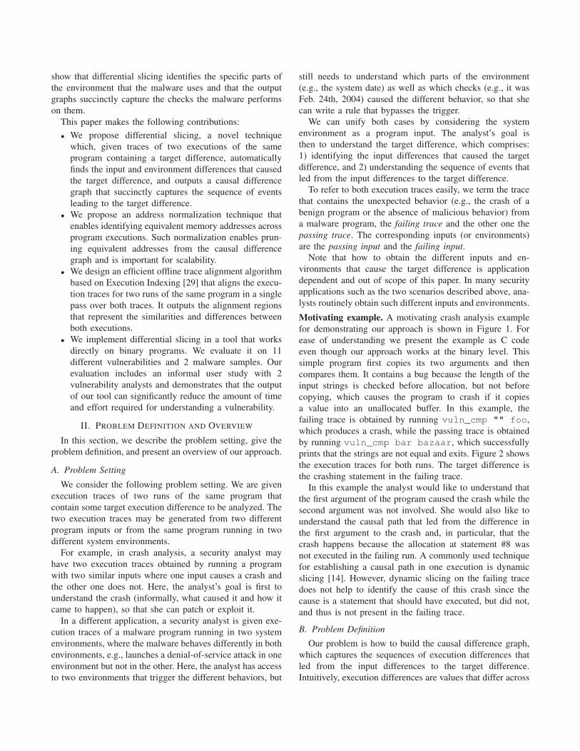
a value into an unallocated buffer. In this example, the

failing trace is obtained by running vuln_cmp "" foo,

which produces a crash, while the passing trace is obtained

by running vuln_cmp bar bazaar, which successfully

prints that the strings are not equal and exits. Figure 2 shows

the execution traces for both runs. The target difference is

the crashing statement in the failing trace.

In this example the analyst would like to understand that

the first argument of the program caused the crash while the

second argument was not involved. She would also like to

understand the causal path that led from the difference in

the first argument to the crash and, in particular, that the

crash happens because the allocation at statement #8 was

not executed in the failing run. A commonly used technique

for establishing a causal path in one execution is dynamic

slicing [14]. However, dynamic slicing on the failing trace

does not help to identify the cause of this crash since the

cause is a statement that should have executed, but did not,

and thus is not present in the failing trace.

B. Problem Definition

Our problem is how to build the causal difference graph,

which captures the sequences of execution differences that

led from the input differences to the target difference.

Intuitively, execution differences are values that differ across

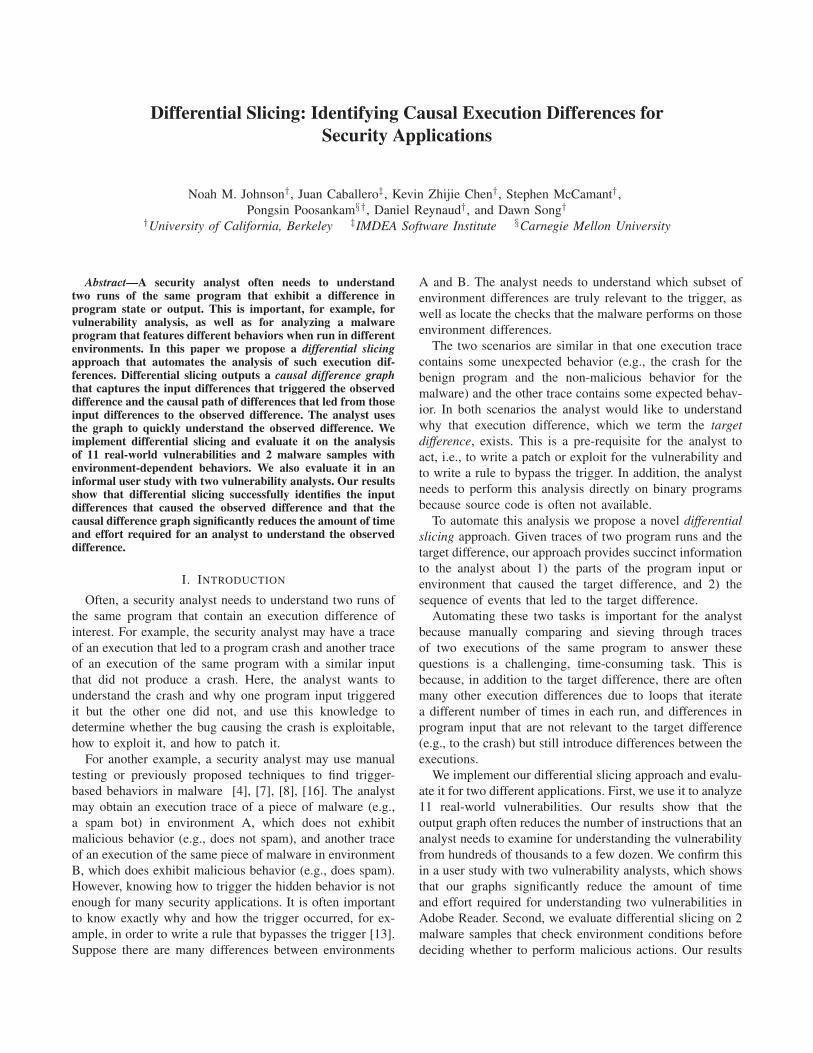
1 char ∗ s1=NULL, ∗ s2=NULL;2 i n t main ( i n t argc , char ∗∗ a rgv ) {3 i f ( a r g c < 3)4 re turn 1 ;5 i n t l e n1 = s t r l e n ( a rgv [ 1 ] ) ;6 i n t l e n2 = s t r l e n ( a rgv [ 2 ] ) ;7 i f ( l e n1 )8 s1 = ( char ∗ ) ma l l oc ( l e n1 ) ;9 i f ( l e n2 )

10 s2 = ( char ∗ ) ma l l oc ( l e n2 ) ;11 s t r n c p y ( s1 , a rgv [ 1 ] , l e n1 ) ;12 s t r n c p y ( s2 , a rgv [ 2 ] , l e n2 ) ;13 i f ( s t r cmp ( s1 , s2 ) != 0 )14 p r i n t f ( ” S t r i n g s a r e no t e qu a l \n” ) ;15 re turn 0 ;16 }

Figure 1: Motivating example program, vuln cmp.c.

runs, or statements that executed in only one run. However,

determining that a value differs, or that a statement appears

only in one trace, requires first establishing correspondence

between statements in both traces. This is difficult because

the same statement may appear multiple times in an ex-

ecution due to loops, recursive functions, or invocations

of the same function in different contexts. The process of

establishing such correspondence is called trace alignment

and is a pre-requisite for identifying execution differences.

Trace alignment. Given passing (p) and failing (f ) traces

of size n and m instructions, respectively, we say that a

pair of statements from these traces (px, fy) s.t. x ∈ [1, n],y ∈ [1,m] are aligned if they correspond to each other. We

say that a statement in one trace is disaligned if it has no

corresponding statement in the other trace, which we rep-

resent with a pair (px,⊥) or (⊥,fy). Trace alignment marks

each statement in both traces as either aligned or disaligned.

Since execution traces can contain many statements, we

group them together into regions based on their alignment.

An aligned region is a maximal sequence of consecutive

aligned statements: (px, fy), (px+1, fy+1), . . . , (px+k, fy+k)s.t. ∀i ∈ [0, k] px+i, fy+i 6=⊥. Similarly, a disaligned region

is a maximal sequence of consecutive disaligned statements:

(px,⊥), . . . , (px+k,⊥) or (⊥, fx), . . . , (⊥, fx+k).

A disaligned region is always immediately preceded by

an aligned region. We term the last statement in an aligned

region a divergence point because it creates a disaligned

region by transferring control to different statements in both

traces. Given a disaligned region, we call the divergence

point of the immediately preceding aligned region, the

immediate divergence point.

Figure 2 shows the alignment for our motivating exam-

ple and illustrates these definitions. The figure shows that

the two executions are aligned until branch statement #7

executes. Here, statements #3–#7 in each trace form an

aligned region. Branch statement #7 is a divergence point;

it evaluates to true in the passing run and to false in the

Passing run

/* argc = 3 */3: if(argc<3) /* argv[1] = "bar" */5: int len1 = strlen(argv[1]) /* argv[2] = "bazaar" */6: int len2 = strlen(argv[2]) /* len1 = 3 */7: if (len1)

/* len2 = 6 */9: if (len2)/* len2 = 6 */ 10: s2 = (char *)malloc(len2)/* s1 = (ptr to 3-byte buffer), argv[1] = "bar", len1 = 3 */11: strncpy(s1, argv[1], len1)

crash

/* len1 = 3 */8: s1 = (char *)malloc(len1)

/* s1 = (ptr to 6-byte buffer), argv[2] = "bazaar", len2 = 6 */12: strncpy(s2, argv[2], len2)...15: return 0

V

V

V

F

V

V

V

F

F

Failing run

_ /* argc = 3 */3: if(argc<3)/* argv[1] = "" */5: int len1 = strlen(argv[1])/* argv[2] = "foo" */6: int len2 = strlen(argv[2])/* len1 = 0 */7: if (len1)

/* len2 = 3 */9: if (len2)/* len2 = 3 */10: s2 = (char *)malloc(len2)/* s1 = NULL, argv[1] = "", len1 = 0 */11: strncpy(s1, argv[1], len1)

Figure 2: Traces and alignment for motivating example.

V and F refer to value and flow differences, respectively

(Section II-B).

failing run, creating a disaligned region because statement

#8 executes in the passing run but not in the failing run (an

execution omission). The two executions realign at statement

#9 and remain aligned until statement #11 produces the crash

in the failing trace. Thus, statements #9–#11 form another

aligned region.

Execution differences. Given two aligned executions, we

define two types of execution differences: flow differences

and value differences. A flow difference is simply a dis-

aligned statement. For example, statement #8 in Figure 2 is

a flow difference.

A value difference is a variable used in an aligned

statement that has a different value in both executions. For

example, the len2 variable in statement #10 in Figure 2

is a value difference because it has value 6 in the passing

run and value 3 in the failing run. We say that a statement

has a value difference when it uses one or more variables

that are value differences. For example, statement #11 in

Figure 2 has 3 value differences: s1, argv[1], and s1.

Each statement in Figure 2 is marked on the left with a V to

indicate that it contains a value difference, an F to indicate

that it is a flow difference, or - otherwise.

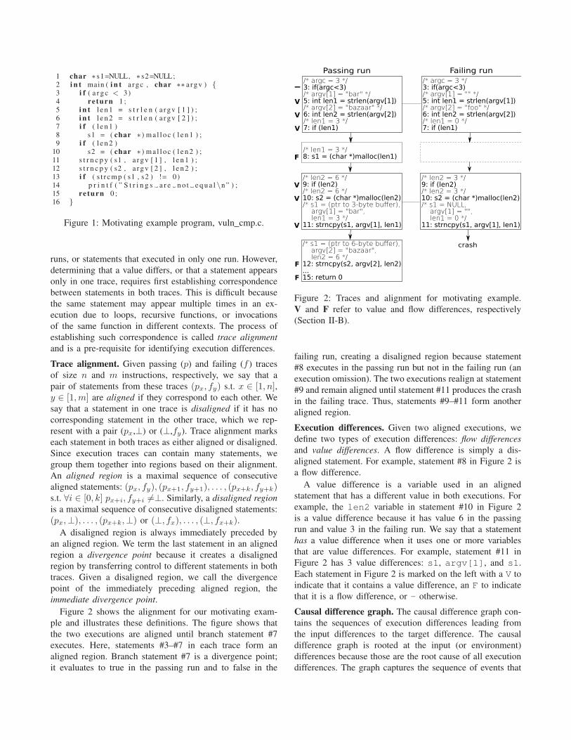
Causal difference graph. The causal difference graph con-

tains the sequences of execution differences leading from

the input differences to the target difference. The causal

difference graph is rooted at the input (or environment)

differences because those are the root cause of all execution

differences. The graph captures the sequence of events that

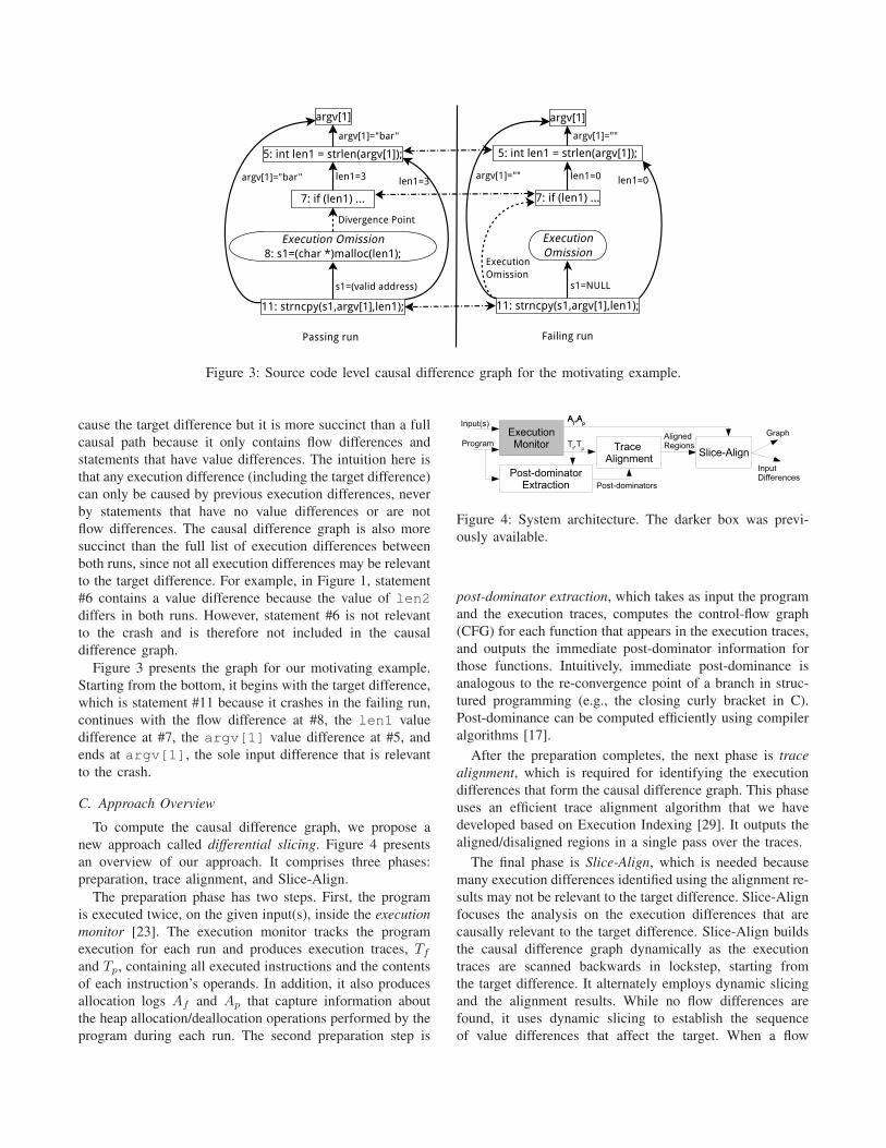
Figure 3: Source code level causal difference graph for the motivating example.

cause the target difference but it is more succinct than a full

causal path because it only contains flow differences and

statements that have value differences. The intuition here is

that any execution difference (including the target difference)

can only be caused by previous execution differences, never

by statements that have no value differences or are not

flow differences. The causal difference graph is also more

succinct than the full list of execution differences between

both runs, since not all execution differences may be relevant

to the target difference. For example, in Figure 1, statement

#6 contains a value difference because the value of len2

differs in both runs. However, statement #6 is not relevant

to the crash and is therefore not included in the causal

difference graph.

Figure 3 presents the graph for our motivating example.

Starting from the bottom, it begins with the target difference,

which is statement #11 because it crashes in the failing run,

continues with the flow difference at #8, the len1 value

difference at #7, the argv[1] value difference at #5, and

ends at argv[1], the sole input difference that is relevant

to the crash.

C. Approach Overview

To compute the causal difference graph, we propose a

new approach called differential slicing. Figure 4 presents

an overview of our approach. It comprises three phases:

preparation, trace alignment, and Slice-Align.

The preparation phase has two steps. First, the program

is executed twice, on the given input(s), inside the execution

monitor [23]. The execution monitor tracks the program

execution for each run and produces execution traces, Tf

and Tp, containing all executed instructions and the contents

of each instruction’s operands. In addition, it also produces

allocation logs Af and Ap that capture information about

the heap allocation/deallocation operations performed by the

program during each run. The second preparation step is

Figure 4: System architecture. The darker box was previ-

ously available.

post-dominator extraction, which takes as input the program

and the execution traces, computes the control-flow graph

(CFG) for each function that appears in the execution traces,

and outputs the immediate post-dominator information for

those functions. Intuitively, immediate post-dominance is

analogous to the re-convergence point of a branch in struc-

tured programming (e.g., the closing curly bracket in C).

Post-dominance can be computed efficiently using compiler

algorithms [17].

After the preparation completes, the next phase is trace

alignment, which is required for identifying the execution

differences that form the causal difference graph. This phase

uses an efficient trace alignment algorithm that we have

developed based on Execution Indexing [29]. It outputs the

aligned/disaligned regions in a single pass over the traces.

The final phase is Slice-Align, which is needed because

many execution differences identified using the alignment re-

sults may not be relevant to the target difference. Slice-Align

focuses the analysis on the execution differences that are

causally relevant to the target difference. Slice-Align builds

the causal difference graph dynamically as the execution

traces are scanned backwards in lockstep, starting from

the target difference. It alternately employs dynamic slicing

and the alignment results. While no flow differences are

found, it uses dynamic slicing to establish the sequence

of value differences that affect the target. When a flow

difference is encountered, e.g., an execution omission, it

uses the alignment results to identify the divergence point

that dominates the disaligned regions. Once found, dynamic

slicing is used to capture the value differences that caused

that divergence point until another flow difference is found.

This sequence repeats until the input differences are reached.

Graph layers. The resulting Basic graph contains only the

execution differences that are relevant to the target differ-

ence. Disaligned regions in the Basic graph are summarized

as a single node to help the analyst quickly understand which

flow differences are relevant to the target difference and

why they happened. An analyst who is interested in what

happened in those disaligned regions can request what we

call an Enhanced graph, which expands the Basic graph

by incorporating the relevant dependencies in a disaligned

region. Such multi-layer approach gives the analyst a small

Basic graph that often suffices for analysis as well as the

ability to produce finer-grained Enhanced graphs for specific

divergence regions.

Address normalization. An important feature for the scal-

ability of our approach is the ability to prune edges in the

graph when an operand of an aligned instruction is not a

value difference. Without pruning, the graph can quickly

explode in size because the nodes that explain how those

identical values were generated need to be included, even

if identical values cannot be the cause of an execution

difference. However, many operands in the execution contain

pointers that may have different values across runs but are

still equivalent to each other (e.g., the objects pointed to

are equivalent). We have developed an address normaliza-

tion technique that identifies operands that hold equivalent

pointers. By pruning those operands we obtain graphs that

are in some cases one to two orders of magnitude smaller

than without the address normalization.

Implementation. We have implemented differential slicing

in approximately 6k lines of Objective Caml code. The

trace alignment and post-dominator modules are written in

4k lines of code (excluding the call stack code and APIs

for creating control flow graphs, which we adapted for our

system from previous work). The Slice-Align module is

written in 2k lines of code. The execution monitor was

previously available [23].

III. TRACE ALIGNMENT

The first step in our differential slicing approach is to

align the failing and passing execution traces to identify

similarities and differences between the executions. Our

trace alignment algorithm builds on the previously proposed

Execution Indexing technique [29], where an execution

index uniquely identifies a point in an execution and can be

used to establish correspondence across executions. Unlike

previous work, we propose an efficient offline alignment

trace algorithm that requires just a single pass over the traces

and works directly on binaries without access to source code.

In this section, we first provide background information

on the Execution Indexing technique in Section III-A and

then we describe our trace alignment algorithm in Sec-

tion III-B.

A. Background: Execution Indexing

Execution Indexing captures the structure of the program

at any given point in the execution, uniquely identifying

the execution point, and uses that structure to establish a

correspondence between execution points across multiple

executions of the program [29]. Compared to using static

program points to establish a correspondence, Execution

Indexing is able to align points inside loops and functions

with multiple call sites.

Xin et al. propose an online algorithm to compute the

current execution index as the execution progresses, which

uses an indexing stack, where an entry is pushed to the

stack when a branch or method call is seen in the execution,

and an entry is popped from the stack if the immediate

post-dominator of the branch is executed or the method

returns. Note that a statement may be the immediate post-

dominator of multiple branches or call statements and can

thus pop multiple entries from the stack. For example, a

return instruction is the immediate post-dominator of all the

branches in the stack for the current function invocation. Xin

et al. also propose optimizations to minimize the number

of push and pop operations for cases that include, among

others, avoiding instrumenting instructions with a single

static control dependence and using counters for loops or

repeated predicates.

Execution Indexing captures the structure of the execution

starting at an execution point that is called an anchor point.

To compare the structure of two executions, Execution In-

dexing requires as input a point in each execution considered

semantically equivalent (i.e., already aligned). These can be

automatically defined or provided by the analyst. We explain

our anchor point selection in Section III-B.

B. Trace Alignment Algorithm

Our trace alignment algorithm compares two execution

traces representing different runs of the same program. There

are two main issues in pairwise trace alignment: designing

an efficient algorithm that scales to large traces, and selecting

anchor points. We discuss both issues next.

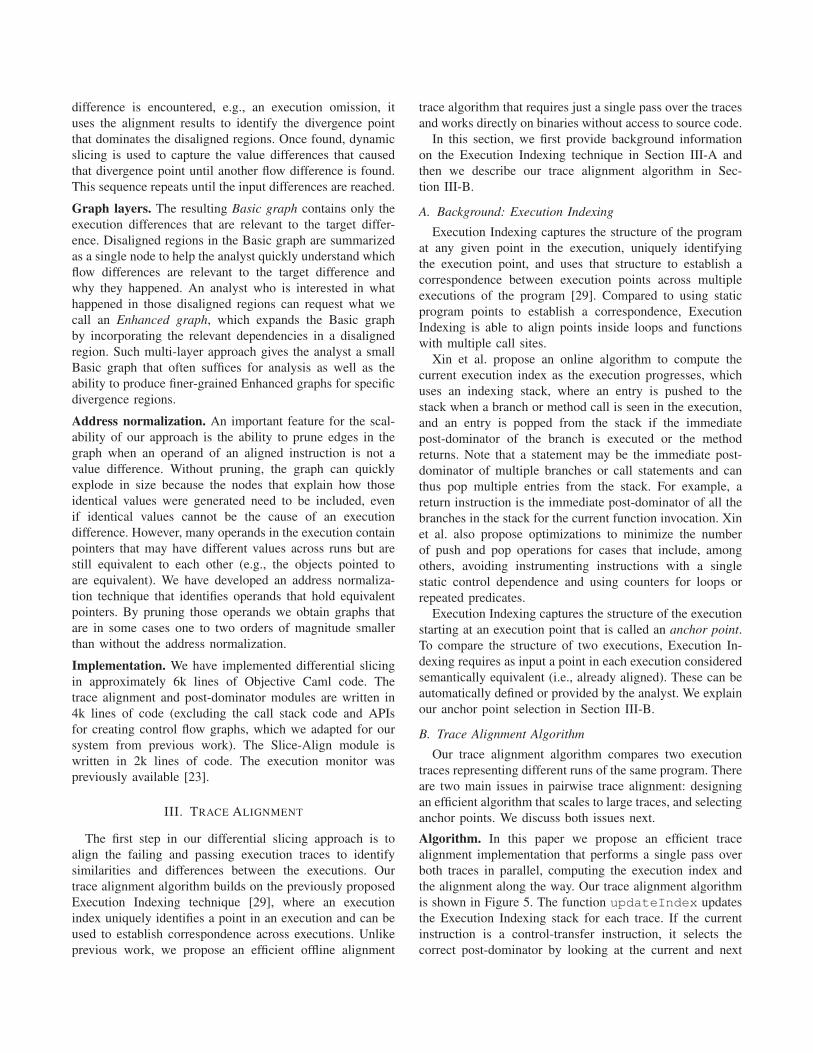
Algorithm. In this paper we propose an efficient trace

alignment implementation that performs a single pass over

both traces in parallel, computing the execution index and

the alignment along the way. Our trace alignment algorithm

is shown in Figure 5. The function updateIndex updates

the Execution Indexing stack for each trace. If the current

instruction is a control-transfer instruction, it selects the

correct post-dominator by looking at the current and next

Input: A0, A1 // anchor points

Output: RL // list of aligned and disaligned regions

EI0, EI1 : execution index stacks ← Stack.empty();insn0, insn1 ← A0, A1; // current instructions

RL← ∅;while insn0, insn1 6=⊥ do

cr ← regionBegin(insn0, insn1, aligned)// Aligned-Loop: Traces aligned. Walk until disaligned

while EI0 = EI1 doforeach i ∈ 0, 1 do

EIi ← updateIndex(EIi, insni);cr ← regionExtend(insni, cr);insni++;

endendRL← RL ∪ cr;cr ← regionBegin(insn0, insn1, disaligned)// Disaligned-Loop: Traces disaligned. Walk until realigned

while EI0 6= EI1 dowhile |EI0| 6= |EI1| do

j ← (|EI0| > |EI1|) ? 0 : 1;while |EIj | ≥ |EI1−j | do

EIj ← updateIndex(EIj , insnj);cr ← regionExtend(insnj , cr);insnj++;

endend

endRL← RL ∪ cr;

end

Figure 5: Algorithm for trace alignment.

instruction (i.e., the target of the control flow transfer)

and pushes the post-dominator into the stack. While the

current instruction corresponds to the post-dominator at the

top of the stack, it pops it. Our experience shows that

it is important to handle unstructured control flow (e.g.,

setjmp/longjmp), which requires building robust call

stack tracking code [5].

The trace alignment algorithm proceeds as follows. It

starts with both anchor points being processed in the

Aligned-Loop. This loop creates an aligned region by

stepping through both traces until a disaligned instruction

is found. While the Execution Index (EI) for the cur-

rent instruction in each trace (insn0,insn1) is the same,

both instructions are added to the current alignment region

(cr) and the Execution Index is updated for each trace

(updateIndex).

At a divergence point, the current region is added to the

output (RL), a new disaligned region is created (cr) and

Disaligned-Loop is entered. This loop searches for the

realignment point in the two traces. Realignment can only

happen after the top entry (at the time of disalignment)

on the stack has been popped, because in order for the

Execution Indexes to match, any additional entries added

to the stack after this point will first need to be popped.

Intuitively, this means that when the executions diverge, the

first possible place they can realign is at the post-dominator

of the divergence point.

The Disaligned-Loop walks both traces individually

until the top entry in the stack at the time the disalignment

point was found has been removed. If the stacks are equal

at this point, it means that the traces have realigned at the

immediate post-dominator. The current disalignment region

ends and Aligned-Loop continues at this new aligned

point. If the call stacks are unequal in size, the trace with

the larger call stack is traversed until its call stack matches

or falls below the size of the other trace’s call stack. This

process is repeated until the two call stacks are equal in

size. Then, the current Execution Indexes are compared. If

not equal, the Disaligned-Loop repeats, popping the

current top entry until the two stacks are equal in size, then

recomparing the Execution Indexes.

Anchor point selection. To use Execution Indexing for

alignment, we need an anchor point: two instructions (one

in each trace) that are considered aligned. While this may

seem like a circular problem, there are some points in the

execution where we are confident that both executions are

aligned. For example, if we always start tracing a program

at the first instruction for the created process, then we

can select the first instruction in both traces as anchor

points, as they are guaranteed to be the same program point.

Sometimes, starting execution traces from process creation

may produce execution traces that are too large. In those

cases, we can start the traces when the program reads its

first input byte, so the first instruction in each trace is an

anchor point.

IV. SLICE-ALIGN

The trace alignment results capture all flow differences

between both executions and establish instruction correspon-

dence so that value differences in corresponding instructions

can be identified. However, the total number of execution

differences can be large and many of those differences

may not be relevant to the target difference. In this section

we present Slice-Align, a technique to produce the causal

difference graph, which captures only the causal sequences

of execution differences that affected the target difference.

The root differences in the graph correspond to the input

differences that induced the target difference.

A. The Causal Difference Graph

The causal difference graph is a directed graph where

each node in the graph represents an instruction in an

execution trace. The graph has two sets of nodes and

edges: Np, Ep from the passing trace and Nf , Ef from

the failing trace. There are two types of edges: directed

edges representing immediate data and control dependencies

between two instructions in the same trace, and undirected

edges representing that two instructions in different traces

are aligned. Directed edges are labeled to indicate whether

they represent a control or data dependency and, for data

dependencies, which operand the edge corresponds to as

well as the value of the operand in the execution.

Note that an instruction has at most one immediate dy-

namic control dependency, but can have multiple immediate

data dependencies, e.g., one for each operand that it uses

(including memory addressing registers). An operand can

also depend on multiple instructions, for example when each

byte in a 32-bit register was defined at a different instruction.

In these cases, operands are broken into individual bytes

and the edges labeled accordingly, so that the analyst can

differentiate the multiple out-edges of a node.

Layers. The graph has two levels of granularity, depending

on how much information the analyst wants about the

dependencies inside disaligned regions. The Basic graph

summarizes each disaligned region with a single node that

represents all execution differences inside that region. This

layer is intended to help the analyst quickly understand

which disaligned regions are causally related to the target

difference and why they happened.

An analyst may be interested in “zooming in” on one of

those disaligned regions to understand the flow differences

that it contains. For example, for an execution omission

error, the disaligned region in the passing trace may in-

clude the initialization statement that was not executed in

the failing trace. Although the Basic graph captures the

cause of the execution omission, the analyst may also be

interested in looking at the missing initialization. To handle

these situations, Slice-Align provides an option to explicitly

include the causal sequences of execution differences from

one or more specific disaligned regions into the Basic graph,

creating an Enhanced graph.

In the next section we describe the Slice-Align algorithm.

We first describe the algorithm that builds the Basic graph

and then the different handling of the disaligned regions that

is used to build the Enhanced graph.

B. Basic Graph Algorithm

At a high level, the Slice-Align algorithm combines

dynamic slicing with trace alignment. In particular, it uses

backwards dynamic slicing techniques [1], [14], [31] to

identify immediate data dependencies of value differences,

while using the trace alignment results to identify execution

differences. As it traverses the execution traces, it adds

to the graph the value and flow differences with a causal

relationship to the target difference.

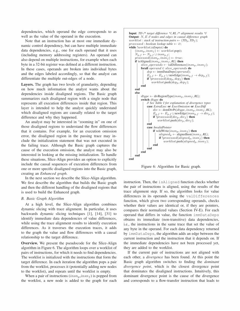
Overview. We present the pseudocode for the Slice-Align

algorithm in Figure 6. The algorithm loops over a worklist of

pairs of instructions, for which it needs to find dependencies.

The worklist is initialized with the instructions that form the

target difference. In each iteration the algorithm pops a pair

from the worklist, processes it (potentially adding new nodes

to the worklist), and repeats until the worklist is empty.

When a pair of instructions (insnp,insnf ) is popped from

the worklist, a new node is added to the graph for each

Input: TD /* target difference */,RL /* alignment results */

Output: N,E // nodes and edges in causal difference graph

worklist : stack of instruction-pairs← (TDp, TDf );processed : boolean lookup table← ∅;while !worklist.isEmpty() do

(insnp, insnf )← worklist.pop();Np,f ← Np,f ∪ insnp,f ;processed(insnp, insnf )← true;if isAligned(insnp, insnf ,RL) then

slice operands← valDifferences(insnp, insnf );forall operand ∈ slice operands do

dep← immDataDeps(operand);Ep,f ← Ep,f ∪ newEdge(insnp,f → depp,f );if !processed(depp, depf ) then

worklist.push(depp, depf );end

endelse

dtype← divRegionType(insnp, insnf ,RL);switch dtype do

// See Table I for explanation of divergence types

case ExtraExec or ExecOmission or ExecDiffdiv ← domDivPt(dtype, insnp, insnf ,RL);Ep,f ← Ep,f ∪ newEdge(insnp,f → divp,f );if !processed(divp, divf ) then

worklist.push(divp, divf );endcase InvalidPointer

if wildWrite(insnp, insnf ) thenalignedp ← alignedInsn(insnf ,RL);if !processed(alignedp, insnf ) then

worklist.push(alignedp, insnf );end

endend

endend

Figure 6: Algorithm for Basic graph.

instruction. Then, the isAligned function checks whether

the pair of instructions is aligned, using the results of the

trace alignment step. If so, the algorithm looks for value

differences in its operands using the valDifferences

function, which given two corresponding operands, checks

whether their values are identical or, if they are pointers,

compares their normalized values (Section IV-E). For each

operand that differs in value, the function immDataDeps

obtains its immediate (non-transitive) data dependencies,

i.e., the instructions in the same trace that set the value of

any byte in the operand. For each data dependency returned

by immDataDeps, the algorithm adds an edge between the

current instruction and the instruction that it depends on. If

the immediate dependencies have not been processed yet,

they are added to the worklist.

If the current pair of instructions are not aligned with

each other, a divergence has been found. At this point the

Basic graph algorithm switches to finding the dominant

divergence point, which is the closest divergence point

that dominates the disaligned instructions. Intuitively, this

dominant divergence point is the cause of the divergence

and corresponds to a flow-transfer instruction that leads to

Case Name Passing Failing

1 Extra Execution Aligned Disaligned

2 Execution Omission Disaligned Aligned

3 Execution Difference Disaligned Disaligned

4 Invalid Pointer Aligned Aligned

4a Wild Read Aligned Aligned4b Wild Write Aligned Aligned

Table I: The divergence types.

two different targets in both executions, for which following

each branch would eventually lead to each of the disaligned

instructions, and for which there is no earlier realignment

point in both executions. Finding the dominant divergence

point comprises five different cases, which we describe next.

Once the dominant divergence point is found, it is added to

the worklist and the algorithm iterates.

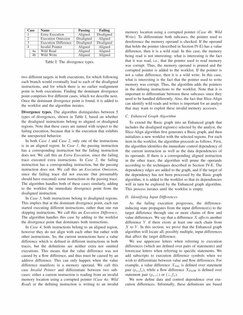
Divergence types. The algorithm distinguishes between 5

types of divergences, shown in Table I, based on whether

the disaligned instructions belong to aligned or disaligned

regions. Note that these cases are named with respect to the

failing execution, because that is the execution that exhibits

the unexpected behavior.

In both Case 1 and Case 2, only one of the instructions

is in an aligned region. In Case 1, the passing instruction

has a corresponding instruction but the failing instruction

does not. We call this an Extra Execution, since the failing

trace executed extra instructions. In Case 2, the failing

instruction has a corresponding instruction, but the passing

instruction does not. We call this an Execution Omission,

since the failing trace did not execute (but presumably

should have executed) some instructions in the passing trace.

The algorithm handles both of these cases similarly, adding

to the worklist the immediate divergence point from the

disaligned instruction.

In Case 3, both instructions belong to disaligned regions.

This implies that at the dominant divergence point, each run

started executing different instructions, rather than one run

skipping instructions. We call this an Execution Difference.

The algorithm handles this case by adding to the worklist

the divergence point that dominates both instructions.

In Case 4, both instructions belong to an aligned region,

however they do not align with each other but rather with

other instructions. So, the current instructions have a value

difference which is defined in different instructions in both

traces, but the definitions are neither extra nor omitted

executions. This means that the value difference was not

caused by a flow difference, and thus must be caused by an

address difference. This can only happen when the value

difference manifests in a memory operand. We call this

case Invalid Pointer and differentiate between two sub-

cases: either a current instruction is reading from an invalid

memory location using a corrupted pointer (Case 4a: Wild

Read) or the defining instruction is writing to an invalid

memory location using a corrupted pointer (Case 4b: Wild

Write). To differentiate both subcases, the pointer used to

dereference the memory operand is checked. If the operand

that holds the pointer (described in Section IV-E) has a value

difference, then it is a wild read. In this case, the memory

being read is not interesting; what is interesting is the fact

that it was read, i.e., that the pointer used to read memory

was corrupt. Thus, the memory operand is pruned and the

corrupted pointer is added to the worklist. If the pointer is

not a value difference, then it is a wild write. In this case,

what is interesting is the fact that the pointer used to write

memory was corrupt. Thus, the algorithm adds the pointers

in the defining instructions to the worklist. Note that it is

important to differentiate between these subcases since they

need to be handled differently. Also, the fact that Slice-Align

can identify wild reads and writes is important for an analyst

that may want to exploit these invalid memory accesses.

C. Enhanced Graph Algorithm

To extend the Basic graph into an Enhanced graph that

includes the disaligned region(s) selected by the analyst, the

Slice-Align algorithm first generates a Basic graph, and then

initializes a new worklist with the selected regions. For each

item in the worklist, the algorithm proceeds as follows. First,

the algorithm identifies the immediate control dependency of

the current instruction as well as the data dependencies of

its operands. If there is a corresponding aligned instruction

in the other trace, the algorithm will prune the operands

according to the techniques described in Section IV-E. The

dependency edges are added to the graph, and if the target of

the dependency has not been processed by the Basic graph

algorithm, it is added to the worklist so that its dependencies

will in turn be explored by the Enhanced graph algorithm.

This process iterates until the worklist is empty.

D. Identifying Input Differences

As the failing execution progresses, the difference-

inducing state propagates from the input difference(s) to the

target difference through one or more chains of flow and

value differences. We say that a difference X affects another

difference Y if there exists at least one such chain from

X to Y . In this section, we prove that the Enhanced graph

algorithm will locate all, possibly multiple, input differences

that affect the target difference.

We use uppercase letters when referring to execution

differences (which are defined over pairs of statements) and

lowercase letters when referring to specific statements. We

add subscripts to execution difference symbols when we

wish to differentiate between value and flow differences. For

example, a value difference XVAL is defined over statement

pair (px,fx), while a flow difference XFLOW is defined over

statement pair (px,⊥) or (⊥,fx).

We now define data and control dependence over exe-

cution differences. Informally, these definitions are based

on their analogs in dynamic program slicing (i.e., edges in

the program dependence graph [9], [12]), except they are

defined with respect to pairs of execution statements rather

than statements from a single execution.

Let X and Y be two distinct execution differences. We

say Y is data dependent on X (denoted YDD−−→ X) iff

pydd−→ px ∧ fy

dd−→ fx. Similarly, Y is control dependent

on X (denoted YCD−−→ x) iff py

cd−→ px ∧ fy

cd−→ fx. If X

or Y are flow differences, then only the predicate for the

flow-differing statement needs to hold (equivalently, we say

⊥dd|cd−−−→ ⊥ and ∀x ⇒ ⊥

dd|cd−−−→ x ∧ x

dd|cd−−−→ ⊥).

We now show that even though we prune many irrelevant

execution differences, the input differences are guaranteed

to be present in the causal difference graph.

Theorem 1: Any input difference that affects the target

difference will appear in the causal difference graph.

Proof: Our proof is by induction over the legal tran-

sitions between execution differences (e.g., edges in the

graph). In particular, we demonstrate that for any transition

from X to Y (i.e., YDD|CD−−−−−→ X), if Y appears in the

worklist, then X will be identified by the algorithm and

added to the worklist.

In the base case, if the input difference appears in the

worklist then, by definition of input difference, there are

no more dependencies and the algorithm completes success-

fully.

For the inductive step, we enumerate all transitions from

X to Y (i.e., YVAL|FLOWDD|CD−−−−−→ XVAL|FLOW) that may occur

along the causal path, and explain how the Slice-Align

algorithm identifies the source of the transition in each case.

First, consider a transition from a value difference XVAL

to another value difference YVAL. Note that YVAL cannot be

control dependent on XVAL since a value difference at branch

XVAL would necessarily imply a control flow difference, but

by the definition of value difference, the statements in YVAL

are aligned. Thus, we need only consider the dependency

YVALDD−−→ XVAL. If YVAL appears in the worklist, then XVAL

will be identified by the data slicing in the Basic graph

algorithm, which adds the data dependencies of every value

difference to the worklist.

Next, consider a transition from a value difference XVAL

to a flow difference YFLOW. This transition can be caused

by either a data dependency or a control dependency. For

a control dependency (YFLOWCD−−→ XVAL), XVAL must be a

divergence point, by the above argument. Then XVAL will

be identified by the Basic graph algorithm, which adds the

divergence point of flow differences to the worklist. For a

data dependency (YFLOWDD−−→ XVAL), the full slicing step of

the Enhanced graph algorithm will add XVAL to the worklist.

Note that the wild write processing (Case 4b in Table I)

does not handle this situation since it applies only to aligned

statements.

The third case is a flow difference XFLOW to a value

difference YVAL. Note that an aligned statement (e.g. value

difference) cannot be control dependent on a flow difference,

so here we need only consider the case of data dependency

(YVALDD−−→ XFLOW). Intuitively, this type of transition means

that a disaligned statement wrote a value which was read by

the program after realignment (e.g., an execution omission).

Like the first case, XFLOW will be identified by the Basic

graph algorithm since it represents a data dependency where

the source is a value difference.

Finally, consider the case of a flow difference XFLOW to

a flow difference YFLOW. This transition could represent a

data dependency or a control dependency. In either case,

the full slicing step of the Enhanced graph algorithm will

add XFLOW to the worklist.

Our induction hypothesis guarantees that for any node Y

that already appears in the worklist, the Slice-Align algo-

rithm will eventually reach the head of all causal difference

paths through Y . By definition of the affects relationship,

there must exist at least one causal difference path from each

input difference to the target difference. Thus, the proof is

complete by noting that the Slice-Align algorithm adds the

target difference to the initial worklist.

E. Extended Pruning with Address Normalization

An important feature for the scalability of Slice-Align is

the ability to prune edges in the graph when an operand of

an aligned instruction has the same value in both execution

traces. Without pruning, the graph may explode in size be-

cause the nodes that explain how those identical values were

generated need to be included, even if identical values cannot

be the cause of other execution differences. A basic approach

is to prune an operand when its corresponding operand in the

other execution has the same value. However, such pruning

is limited because many operands contain pointers that may

not have identical values between executions but are still

equivalent to each other (e.g., point to equivalent objects).

To address this problem, we use a memory normalization

technique that extends the basic pruning to include equiv-

alent pointers, even if they have different values. This ex-

tended pruning identifies operands that hold pointers, applies

pruning based on the normalized addresses of those pointers,

and prunes other operands by direct value comparison.

Recall that the address of a memory operand in an x86

instruction is computed as: address = base + (index *

scale) + displacement, where the scale and the displacement

are constants and the base and index values are stored in

registers. The base register value and displacement can both

be pointers, as can the index register value if the scale equals

1. The first step to prune a pointer is to identify where it is

stored. For this, we simply select the largest of the three as

the candidate pointer for the operand.

If the candidate pointer is the offset then we are done,

as it is a constant with no further dependencies. Otherwise,

our memory normalization tries to determine whether the

pointers, stored in the index or base register, are equivalent in

the two executions. This process, described next, comprises

two steps. First, each pointer is classified as a heap pointer,

stack pointer, or data section pointer. If both pointers have

the same classification, a specific normalization rule for that

class is applied.

Heap pointer pruning. Direct comparison of heap pointers

often fails because equivalent allocations can return different

pointers. The first step in heap pointer pruning is to check

whether the value of the candidate pointer in each trace

belongs to a live heap buffer. For this, during program

execution the execution monitor produces an allocation log

that captures the dynamic memory allocations/deallocations

performed by the program. We have implemented an API

that reads this allocation log and can answer for a given

memory address and a given point in the execution, whether

there is any live buffer that contains the address. If so, the

API provides the buffer information, including the buffer

start address, the buffer size, and the allocation site (i.e., the

counter of the allocation’s call instruction).

If both candidate pointers point to the heap, we try to

prune them. The key intuition to normalize heap addresses

is that an allocation invocation that is aligned returns an

equivalent pointer in each execution. More specifically, we

prune a candidate heap pointer if: 1) the allocation site for

the live buffers that contain the pointed-to addresses are

aligned, and 2) the offset of those pointed-to addresses, with

respect to the start address of the live buffer they belong

to, is the same. If both properties are satisfied, the register

holding the pointer is pruned.

Since the allocation log starts at process creation but

the trace starts when the first input byte is read, a special

case may happen where the allocation site returned for a

live buffer is not present in the trace and no alignment

information is available for it. In this situation we apply

a more aggressive pruning that assumes the above condition

1) is true and prunes if condition 2) is satisfied.

Stack pointer pruning. Direct comparison of stack pointers

may fail because each thread of a process has a different

stack and because the base address of the stack (highest stack

address) can be randomized using Address Space Layout

Randomization (ASLR) [3]. To check whether the value

of the candidate pointers point to the stack, the range of

stack addresses accessed by each program thread in the

execution trace is computed and rounded to the nearest

page boundaries. The candidate pointer points to the stack

if its value is contained in its thread’s stack range. If

both candidates are stack pointers, they are normalized by

subtracting the thread’s stack base address. If the resulting

offsets are identical the register holding the pointer is pruned

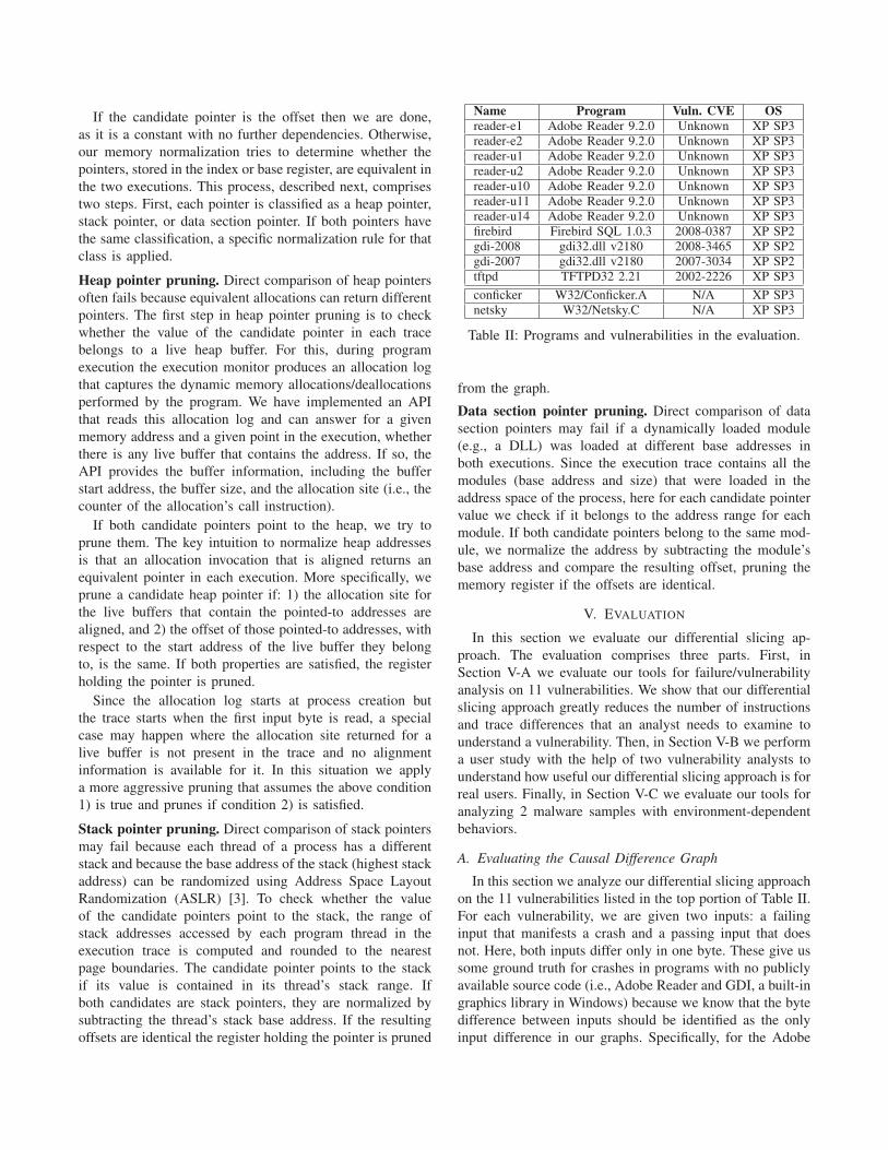
Name Program Vuln. CVE OS

reader-e1 Adobe Reader 9.2.0 Unknown XP SP3

reader-e2 Adobe Reader 9.2.0 Unknown XP SP3

reader-u1 Adobe Reader 9.2.0 Unknown XP SP3

reader-u2 Adobe Reader 9.2.0 Unknown XP SP3

reader-u10 Adobe Reader 9.2.0 Unknown XP SP3

reader-u11 Adobe Reader 9.2.0 Unknown XP SP3

reader-u14 Adobe Reader 9.2.0 Unknown XP SP3

firebird Firebird SQL 1.0.3 2008-0387 XP SP2

gdi-2008 gdi32.dll v2180 2008-3465 XP SP2

gdi-2007 gdi32.dll v2180 2007-3034 XP SP2

tftpd TFTPD32 2.21 2002-2226 XP SP3

conficker W32/Conficker.A N/A XP SP3

netsky W32/Netsky.C N/A XP SP3

Table II: Programs and vulnerabilities in the evaluation.

from the graph.

Data section pointer pruning. Direct comparison of data

section pointers may fail if a dynamically loaded module

(e.g., a DLL) was loaded at different base addresses in

both executions. Since the execution trace contains all the

modules (base address and size) that were loaded in the

address space of the process, here for each candidate pointer

value we check if it belongs to the address range for each

module. If both candidate pointers belong to the same mod-

ule, we normalize the address by subtracting the module’s

base address and compare the resulting offset, pruning the

memory register if the offsets are identical.

V. EVALUATION

In this section we evaluate our differential slicing ap-

proach. The evaluation comprises three parts. First, in

Section V-A we evaluate our tools for failure/vulnerability

analysis on 11 vulnerabilities. We show that our differential

slicing approach greatly reduces the number of instructions

and trace differences that an analyst needs to examine to

understand a vulnerability. Then, in Section V-B we perform

a user study with the help of two vulnerability analysts to

understand how useful our differential slicing approach is for

real users. Finally, in Section V-C we evaluate our tools for

analyzing 2 malware samples with environment-dependent

behaviors.

A. Evaluating the Causal Difference Graph

In this section we analyze our differential slicing approach

on the 11 vulnerabilities listed in the top portion of Table II.

For each vulnerability, we are given two inputs: a failing

input that manifests a crash and a passing input that does

not. Here, both inputs differ only in one byte. These give us

some ground truth for crashes in programs with no publicly

available source code (i.e., Adobe Reader and GDI, a built-in

graphics library in Windows) because we know that the byte

difference between inputs should be identified as the only

input difference in our graphs. Specifically, for the Adobe

NameTotal instructions Disaligned instructions Disaligned regionsPassing Failing Passing Failing All Slice-Align

reader-e1 2,800,163 1,819,714 1,307,465 327,016 983 471

reader-e2 1,616,642 1,173,531 446,273 3,162 75 5

reader-u1 2,430,400 1,436,993 2,034,582 1,041,175 111 32

reader-u2 1,921,514 1,053,840 656,183 14,586 38 23

reader-u10 408,618 272,994 144,517 8,893 39 4

reader-u11 1,868,942 1,112,828 1,504,189 748,075 389 235

reader-u14 1,194,053 155,906 601,789 119,085 524 59

tftpd 626,622 350,323 415,086 138,787 87 4

firebird 6,698 1,282 5,551 135 4 4

gdi-2008 42,124 4,310 38,743 929 1 1

gdi-2007 36,792 4,310 33,508 1,026 1 1

Table III: Total disaligned instructions and regions compared with disaligned regions in graph.

NameBasic pruning Extended pruning

Pass Fail # IDiff Pass Fail # IDiff

reader-e1 3,651 3,616 7 2,324 2,292 7

reader-e2 4,854 4,853 21 81 84 1

reader-u1 2,753 2,751 13 204 201 1

reader-u2 135 135 1 100 100 1

reader-u10 45 43 1 36 34 1

reader-u11 1,584 1,562 1 1,158 1,135 1

reader-u14 1,714 1,695 6 425 420 1

tftpd 254 254 1 254 254 1

firebird 45 46 1 45 46 1

gdi-2008 100 101 1 96 97 1

gdi-2007 11 12 1 7 8 1

Table IV: Causal difference graph evaluation. The Extended pruning column corresponds to the size of the output graph.

Reader and GDI vulnerabilities, the input PDF or WMF files

have only one byte with a different value, and for the tftpd

and firebird vulnerabilities, the passing input is one byte

shorter than the failing one.

Relevant execution differences. The first step of our differ-

ential slicing approach is to align the two traces. As a prepa-

ration step, since only one thread is involved in the crashes

that we evaluate, we extract the relevant thread from each

trace, creating two single-threaded traces. After aligning the

execution traces, we count the number of disaligned regions

(Column Disaligned regions (All) in Table III). Next, we

generate the causal difference graph for each vulnerability

and count the number of disaligned regions in the graph

(Column Disaligned regions (Slice-Align)). The results show

that for the more complex Adobe and tftpd examples, which

come from larger execution traces (shown later in Table V),

the number of disaligned regions in the graph is only

4%-48% of the total number of disaligned regions. Thus,

our differential slicing approach removes a large number

of disaligned regions that are not relevant to the crash. For

the smaller examples (firebird and both GDI vulnerabilities),

the number of total disaligned regions is small enough that

all of them are relevant to the crash. Even if the graph

does not remove disaligned regions in these cases, it still

provides causality information to the analyst and prunes

away many unrelated nodes in those regions that have no

value difference.

The causal difference graphs for reader-e1, -u2, -u10,

-u11, and -u14 identify execution omission errors. This

means that for those vulnerabilities, the causal path returned

by a dynamic slice (data and control dependencies) on the

crashing instruction in the failing trace would not make it

back to the input differences, as relevant statements are not

present in the failing trace.

Graph size. Table IV presents the evaluation of the graph

size in three situations. For each situation, the Pass and Fail

columns show the total number of nodes in the passing and

failing graphs, respectively, and the # IDiff column shows the

number of input differences (i.e., root nodes) in the graph.

The Basic pruning columns show the graph sizes when

only direct value comparisons between operands are used to

identify value differences. The Extended pruning columns

show the graph sizes when we incorporate address nor-

malization so that equivalent pointers can also be pruned.

Note that the Extended pruning columns correspond to

the actual output of our tool. The results show that for

the Adobe Reader experiments, the address normalization

greatly improves the pruning. In some experiments (namely,

reader-e2 and reader-u1), extended pruning reduces the

number of nodes in the graph by between one to two orders

of magnitude. Additionally, the results for the reader-e2, -u1,

and -u14 experiments show that the address normalization

often reduces the number of false positive input differences.

For the rest of the experiments, basic and extended pruning

achieve comparable results.

As expected, for the programs that take a file as input

(Adobe, GDI), where the only difference between the pass-

ing and failing inputs is the value of one byte, the graph

captures that the input difference is the byte that differs

between the program inputs. Note that for reader-e1, the

graph also identifies six additional input differences (i.e.

false positives). This is likely due to the conservative nature

of our pruning techniques, which are designed to minimize

incorrect pruning which might prevent the causal graph from

reaching the correct input differences.

In the remainder of this section, we detail how the causal

difference graph helps an analyst in the Tfptd and Firebird

vulnerabilities, describe results for inputs with multi-byte

differences, and present a performance evaluation.

Tfptd. For the tftpd vulnerability there is only one input

difference in the graph, which captures that byte 245 in the

received network data has value 0x7a in the failing trace and

0x00 in the passing trace. The fact that if byte 245 was a null

terminator the program would not crash is an immediate red

flag for an analyst, because it is common in buffer overflows

that an application reads input until it finds a delimiter (0x00

is the string delimiter). If the delimiter appears beyond the

length of the buffer and the program does not check this, an

overflow occurs, which is what happens in this case.

Firebird. For the firebird vulnerability there is only one

input difference in the graph. Surprisingly, the input dif-

ference does not correspond to any values in the received

network data, rather, it corresponds to the return value of the

ws2_32.dll::recv function, which corresponds to the

the size of the received network data. Thus, in this case just

knowing the input difference immediately tells an analyst

that the crash is related to the different size of the input.

Multi-byte input differences. To evaluate whether the

causal difference graph only contains the relevant subset of

input differences in the presence of multiple differences in

the program input, we repeat the reader-u10 experiment four

times. In each experiment, we double the number of bytes

that differ from the failing input by randomly flipping bytes

in the original passing input (making sure the new input

does not crash Adobe Reader). For the four experiments,

the total number of byte differences between the passing and

failing inputs is 4, 8, 16, and 32. We compare the new graphs

with the original one and observe that even if the number

of differences in the program input has increased, the graph

has not changed and the only input difference corresponds

to the original byte difference that caused the crash. Thus,

Slice-Align successfully filters out input differences not

relevant to the crash.

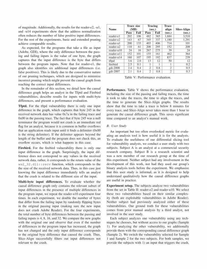
NameTrace size Tracing Trace

(MB) (sec.) align Slice-AlignPass Fail Pass Fail (sec.) (sec.)

reader-e1 202 106 482 365 1,684 3,510

reader-e2 143 67 345 337 1,180 1,291

reader-u1 200 133 403 406 714 101

reader-u2 110 61 208 295 152 208

reader-u10 24 16 267 275 39 24

reader-u11 152 101 155 161 462 364

reader-u14 160 107 195 192 837 239

tftpd 3.6 2.0 13 12 50 12

firebird 2.5 0.1 1 1 1 0.2

gdi-2008 2.4 0.4 2 0.8 2 0.5

gdi-2007 2.1 0.4 2 0.8 2 0.3

Table V: Performance evaluation.

Performance. Table V shows the performance evaluation,

including the size of the passing and failing traces, the time

it took to take the traces, the time to align the traces, and

the time to generate the Slice-Align graphs. The results

show that the time to take a trace is below 8 minutes for

every trace, and Slice-Align never takes more than 1 hour to

generate the causal difference graph. This saves significant

time compared to an analyst’s manual work.

B. User Study

An important but too often overlooked metric for evalu-

ating an analysis tool is how useful it is for the analysts.

To evaluate the usefulness of our differential slicing tool

for vulnerability analysts, we conduct a user study with two

subjects. Subject A is an analyst at a commercial security

research company. Subject B is a research scientist and

was a new member of our research group at the time of

this experiment. Neither subject had any involvement in the

development of this work, nor had they used our group’s

binary analysis tools before the experiment. We emphasize

that this user study is informal, as it is designed to help

understand qualitatively how the causal difference graphs

are useful in practice.

Experiment setup. The subjects analyze two vulnerabilities

from the set in Table II: reader-e2 and reader-u10. We select

these two vulnerabilities based on their similar complex-

ity (both are exploitable vulnerabilities in Adobe Reader).

Neither subject had previously analyzed either of these

vulnerabilities. Our ground truth for these vulnerabilities

comes from prior manual analysis by a third analyst, not

involved in the user study.

Each subject analyzes one vulnerability using any tech-

niques he chooses, but without access to our graphs (Sample

1). For analyzing the other vulnerability, we additionally

provide them with the corresponding causal difference graph

(Sample 2). We switch the vulnerability selected for Sample

1 and Sample 2 for the two subjects. For both samples, we

provide the subjects with 1) an input that triggers the crash,

Subj.

Sample 1 Sample 2(no graph) (Causal difference graph)

sample time found sample time found(hr) cause? (hr) cause?

A reader-e2 13 3 reader-u10 5.5 3

B reader-u10 3 7 reader-e2 3 3

Table VI: Results for user study.

2) a similar input that does not crash and differs from the

crashing input by 1 byte, and 3) the execution traces for

both of these inputs.

We instruct the subjects to stop their analysis once they

understand enough about the vulnerability that they are

confident they know how to exploit or fix it. We also instruct

them to keep track of how long it takes to analyze each

sample, as well as the steps they take during analysis.

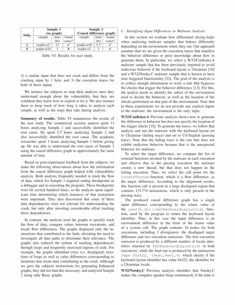
Summary of results. Table VI summarizes the results of

the user study. The commercial security analyst spent 13

hours analyzing Sample 1 and successfully identified the

root cause. He spent 5.5 hours analyzing Sample 2 and

also successfully identified the root cause. The academic

researcher spent 3 hours analyzing Sample 1 before giving

up. He was able to understand the root cause of Sample 2

using the causal difference graph in approximately the same

amount of time.

Based on post-experiment feedback from the subjects, we

make the following observations about how the information

from the causal difference graph helped with vulnerability

analysis. Both analysts frequently needed to track the flow

of data, which for Sample 1 required setting breakpoints in

a debugger and re-executing the program. These breakpoints

were hit several hundred times, so the analysts spent signif-

icant time determining which instances of that instruction

were important. They also discovered that some of these

data dependencies were not relevant for understanding the

crash, but only after investing considerable effort tracking

these dependencies.

In contrast, the analysts used the graphs to quickly track

the flow of data, compare values between executions, and

locate flow differences. The graphs displayed only the in-

structions that contributed to the fault, obviating the need to

investigate all data paths to determine their relevance. The

graphs also reduced the tedium of tracking dependencies

through loops and frequently exercised regions of code. For

example, the graphs identified extra (i.e. disaligned) itera-

tions of loops as well as value differences corresponding to

iterations that wrote data contributing to the crash. Although

we gave the subjects instructions for generating Enhanced

graphs, they did not find this necessary, and analyzed Sample

2 using only Basic graphs.

C. Identifying Input Differences in Malware Analysis

In this section we evaluate how differential slicing helps

when analyzing malware samples that behave differently

depending on the environment where they run. Our approach

assumes that we are given the execution traces that manifest

the behavior difference or prior knowledge about how to

generate them. In particular, we select a W32/Conficker.A

malware sample that has been previously reported to avoid

malicious behavior if the keyboard layout is Ukrainian [18]

and a W32/Netsky.C malware sample that is known to have

time triggered functionality [22]. The goal of the analysis is

to collect enough information to write a rule that bypasses

the checks that trigger the behavior difference [13]. For this,

the analyst needs to identify the subset of the environment

used to decide the behavior, as well as the location of the

checks performed on that part of the environment. Note that

in these experiments we do not provide any explicit inputs

to the malware; the environment is the only input.

W32/Conficker.A Previous analysis shows how to generate

the difference in behavior but does not specify the location of

the trigger checks [18]. To generate the traces, we follow that

analysis and run the malware with the keyboard layout set

to Ukrainian (failing trace) and set to US-English (passing

trace). Note that the failing trace is the one that does not

exhibit malicious behavior because that is the unexpected

behavior for malware.

To select the target difference, we compare the list of

external functions invoked by the malware in each execution

and observe that in the passing execution the malware

creates a new thread, but that does not happen in the

failing execution. Thus, we select the call point for the

CreateThread function, which is a flow difference, as

the target difference. According to the alignment results,

this function call is present in a large disaligned region that

contains 133,774 instructions, which is only present in the

passing trace.

The produced causal difference graph has a single

input difference corresponding to the return value of

the user32.dll::GetKeyboardLayoutList func-

tion, used by the program to return the keyboard layout

identifier. Thus, in this case the input difference is an

environment difference in the form of the return value

of a system call. The graph contains 16 nodes for both

executions, including 3 divergences: the disaligned target

difference and two execution omissions. The first execution

omission is produced by a different number of locale iden-

tifiers returned by GetKeyboardLayoutList in both

executions, while the final one is produced by the instruction

cmpw $0x422, (%edi,%esi,4) which checks if the

keyboard layout identifier has value 0x422, the identifier for

a Ukrainian locale.

W32/Netsky.C Previous analysis identifies that Netsky.C

makes the computer speaker beep continuously if the time is

between 6am and 9am on February 26, 2004 [22], but does

not identify the location of the trigger checks. To generate

the traces, we run the malware with the system local time set

to 7.24am (passing trace) and with the system local time set

to 12.24pm (failing trace), both on February 26, 2004. Based

on the available information, we select the target difference

to be the call point of the Beep function, which only appears

in the passing trace.

The produced causal difference graph has a single in-

put difference that corresponds to the output value of the

kernel32.dll::GetLocalTime system call, used by

the program to obtain the system time. The graph contains

a total of 31 nodes, with one divergence that corresponds

to the disaligned target difference. This disalignment is

produced by different hour digits computed from the result

of GetLocalTime in both executions. In particular, the

graph shows that the malware checks whether the hour digit

is equal to 7 and starts beeping if so. (Note that malware

first checks whether the hour digit is equal to 6, but since

this check is false in both executions, it is not relevant to the

observed malicious behavior and therefore does not appear

in the graph.)

In both of these experiments, the causal difference graph

successfully captures the parts of the environment relevant

to the trigger, as well as the location of the trigger checks,

providing detailed information about the triggering mecha-

nisms which could be used by an analyst, for example, to

construct bypass rules.

VI. RELATED WORK

Differential program analysis. Differential program anal-

ysis refers to analyses pertaining to differences between

two similar programs [27]. Most previous work in this

domain focuses on software engineering applications such

as regression testing [11], [28] and input generation [24].

Most similar to our approach is dual slicing [25], a

technique for debugging concurrency bugs. Like our ap-

proach, dual slicing focuses on execution differences using

two traces. However, dual slicing only applies to execution

differences introduced by different thread schedules, rather

than program input or environment differences. As a result,

the causal paths stop at def-use differences, so dual slicing

is unable to identify the root cause for differences which

are not caused by thread scheduling. Also, the dual slic-

ing algorithm compares values directly across executions,

without any address normalization techniques (such as those

described in Section IV-E). Finally, dual slicing requires

access to source code, while our approach works directly

on binaries.

Also related is work by Sumner and Zhang [20], which

creates a causal path for two executions by first patching

the failing execution dynamically. They do so by modifying

variables and predicates at runtime to produce a passing

execution, a technique first proposed by Zhang et al. to

detect execution omission errors [32]. If such a patch is

found, then both runs are aligned and relevant variables are

identified through value mutations. The main difference with

our technique is that we identify implicit flows and execution

omissions relevant to the target difference by comparing both

executions without re-executing the program.

Trigger detection. There are many existing techniques for

identifying trigger-based behaviors in malware. For example,

[8] presents a technique for identifying time-based behavior

by perturbing the system time of a virtual machine and

observing for different behaviors. Similarly, [4], [16] use

dynamic analysis to explore multiple execution paths in

order to identify hidden behavior in malware. Finally, [7]

presents a more general approach for modeling the behavior

of binary programs in order to statically deduce the presence

of similar functionality in other programs. These techniques

can be used to obtain the execution traces manifesting the

trigger-based behavior, which differential slicing requires.

The benefit of using differential slicing for analyzing a

given trigger-based behavior is that the above techniques

are ill-suited for use by analysts. They can provide coarse-

grained information about the presence or lack of trigger-

based behavior, as well as inputs to trigger the behavior,

but only in specific cases (e.g., time-based triggers) and

with auxiliary information (e.g., hand-crafted signatures of

system calls) can they summarize the trigger conditions in

human-understandable format. Compared to the above tech-

niques, differential slicing outputs a causal difference graph

that provides fine-grained information about the location of

the trigger checks and the parts of the input relevant to the

trigger, in a visual form better suited for a human analyst.

Slicing. One widely used debugging technique proposed by

Weiser is (static) program slicing [26], which produces a

slice containing parts of a program that are relevant to the

computation of a particular value, called the slicing criterion.

Korel and Laski proposed a dynamic version called dynamic

slicing [14], which works on a single execution and outputs

the executed statements relevant to the slicing criterion.

There are four main flavors of dynamic slicing, based on

the dependencies included in the slices: thin slicing [19]

includes a subset of data dependencies, data slicing [31]

includes all data dependencies, full slicing [14] includes

data and control dependencies, and relevant slicing [2],

[10], in addition to data and control dependencies, also

includes predicates, and chains of potential dependencies

rooted at these predicates, whose execution did not affect

the slicing criterion but could have affected it if they had

been evaluated differently. The main difference with our

approach is that differential slicing only considers execution

differences to be relevant to the target difference. Thus,

instead of a causal path of instructions, differential slicing

builds a causal difference graph of execution differences. In

addition, differential slicing can capture execution omission

errors that thin slicing, data slicing, and full slicing cannot

capture because they are not present in the execution, as well

as implicit flows that thin slicing and data slicing cannot

capture. Static and relevant slices will include execution

omissions and implicit flows but will produce large slices.

Delta debugging. Delta debugging is a technique for

isolating and minimizing failure-inducing inputs automati-

cally [30]. Compared to delta debugging, our differential

slicing approach uses information about the execution (i.e.,

is white-box) to identify input differences that are relevant

to the target difference. However, delta debugging can

complement our approach by minimizing inputs such that

they differ by the smallest amount necessary to induce the

observed execution difference (indeed, we generated many

of the inputs for our experiments using a variation of this

technique). Zeller et al. develop a failure analysis approach

that uses delta debugging to compare the states of a faulty

and correct execution at the time the fault is observed [6],

[30]. An important difference with these works is that we

compute the causal difference graph offline, without re-

executing the program in a mutated memory state.

Trace alignment. Xin et al. [29] propose Execution In-

dexing to establish a correspondence between points across

executions based on the structure of the execution. In this

work we use Execution Indexing as a basis for our trace

alignment algorithm. Another offline trace alignment algo-

rithm was proposed by Liang et al. [15] to identify similar

execution traces for fault localization. In contemporaneous

and independent work, Sumner et al. [21] canonicalize the

memory locations and pointer values using memory indices

and apply them to compare memory snapshots of two runs

at selected execution points. Their work is similar to the

technique we use for address normalization, but it requires

access to source code.

VII. CONCLUSION

In this paper we have presented a novel differential slicing

approach that. Given two executions of the same program

and a target difference in those executions, differential slic-

ing produces a causal difference graph. This graph captures

the input differences that caused the target difference, as well

as the causal sequence of execution differences that led the

program from the input differences to the target difference.

Our differential slicing approach comprises two main

steps. First, the two traces are aligned using an efficient

trace alignment algorithm that we have developed based

on Execution Indexing [29]. The alignment results enable

identifying flow and value differences across the executions.

Then, our Slice-Align algorithm outputs a causal difference

graph, which the analyst uses to quickly understand the

target difference.

We have implemented our differential slicing approach

and evaluated it on the analysis of 11 real-world vulnerabil-

ities and two malware samples with environment-dependent

behaviors. Our results show that the causal difference graph

often reduces the number of instructions that an analyst

needs to examine for understanding the target difference

from hundreds of thousands to a few dozen. We confirm this

in a user study with two vulnerability analysts, which shows

that our graphs significantly reduce the amount of time

and effort required for understanding two vulnerabilities in

Adobe Reader.

VIII. ACKNOWLEDGMENTS

We would like to thank Dan Caselden and Charlie Miller

for providing the Adobe Reader samples and for their

valuable feedback on our tool, and Pierre-Marc Bureau for

his help with the Conficker experiment. We are also grateful

to Engin Kirda, David Evans, and the anonymous reviewers

for their valuable comments to improve this manuscript.

This material is based upon work partially supported by

the National Science Foundation under Grants No. 0311808,

No. 0832943, No. 0448452, No. 0842694, No. 0627511,

No. 0842695, No. 0831501, No. 0424422, by the Air

Force Research Laboratory under Grant No. P010071555,

by the Office of Naval Research under MURI Grant No.

N000140911081, and by the MURI program under AFOSR

Grants No. FA9550-08-1-0352 and FA9550-09-1-0539. Juan

Caballero was also partially supported by Grants FP7-

ICT No. 256980, FP7-PEOPLE-COFUND No. 229599, and

Comunidad de Madrid No. S2009TIC-1465. Any opinions,

findings, and conclusions or recommendations expressed in

this material are those of the authors and do not necessarily

reflect the views of the funding agencies.

REFERENCES

[1] H. Agrawal and J. R. Horgan. Dynamic program slicing.ACM SIGPLAN Notices, 25(6), June 1990.

[2] H. Agrawal, J. R. Horgan, E. W. Krauser, and S. London.Incremental regression testing. In ICSM, Montreal, Canada,September 1993.

[3] S. Bhatkar, D. C. DuVarney, and R. Sekar. Address obfus-cation: An efficient approach to combat a broad range ofmemory error exploits. In USENIX Security, Washington,D.C., August 2003.

[4] D. Brumley, C. Hartwig, Z. Liang, J. Newsome,P. Poosankam, D. Song, and H. Yin. Automaticallyidentifying trigger-based behavior in malware. In Bookchapter in ”Botnet Analysis and Defense”, 2007.

[5] J. Caballero. Grammar and Model Extraction for SecurityApplications using Dynamic Program Binary Analysis. PhDthesis, Department of Electrical and Computer Engineering,Carnegie Mellon University, Pittsburgh, PA, September 2010.

[6] H. Cleve and A. Zeller. Locating causes of program failures.In ICSE, Saint Louis, MO, May 2005.

[7] P. M. Comparetti, G. Salvaneschi, E. Kirda, C. Kolbitsch,C. Kruegel, and S. Zanero. Identifying dormant functionalityin malware programs. In Proceedings of the 2010 IEEESymposium on Security and Privacy, SP ’10, pages 61–76,Washington, DC, USA, 2010. IEEE Computer Society.

[8] J. R. Crandall, G. Wassermann, D. A. S. Oliveira, Z. Su,S. Felix, W. Frederic, and T. Chong. Temporal search:Detecting hidden malware timebombs with virtual machines.In Operating Systems Review, pages 25–36. ACM Press,2006.

[9] J. Ferrante, K. J. Ottenstein, and J. D. Warren. The programdependence graph and its use in optimization. ACM Trans.Program. Lang. Syst., 9:319–349, July 1987.

[10] T. Gyimothy, A. Beszedes, and I. Forgacs. An efficientrelevant slicing method for debugging. In ESEC, Toulouse,France, September 1999.

[11] M. J. Harrold, Y. G. Rothermel, Z. K. Sayre, Z. R. Wu,and L. Y. Z. An empirical investigation of the relationshipbetween spectra differences and regression faults. SoftwareTesting, Verification and Reliability, 10:2000, 2000.

[12] S. Horwitz, T. Reps, and D. Binkley. Interprocedural slicingusing dependence graphs. ACM Trans. Program. Lang. Syst.,12:26–60, January 1990.

[13] M. G. Kang, H. Yin, S. Hanna, S. McCamant, and D. Song.Emulating emulation-resistant malware. In VMSec, Chicago,IL, November 2009.

[14] B. Korel and J. Laski. Dynamic program slicing. Info. Proc.Letters, 29(3), October 1988.

[15] G. Liang, A. Roychoudhury, and T. Wang. Accuratelychoosing execution runs for software fault localization. InCC, Vienna, Austria, March 2006.

[16] A. Moser, C. Kruegel, and E. Kirda. Exploring multipleexecution paths for malware analysis. In Proceedings ofthe 2007 IEEE Symposium on Security and Privacy, SP’07, pages 231–245, Washington, DC, USA, 2007. IEEEComputer Society.

[17] S. S. Muchnick. Advanced compiler design and implementa-tion. Morgan Kaufmann, 1997.

[18] P. Porras, H. Saidi, and V. Yegneswaran. A foray intoConficker’s logic and rendezvous points. In LEET, Boston,MA, April 2009.

[19] M. Sridharan, S. J. Fink, and R. Bodik. Thin slicing. InPLDI, San Diego, CA, June 2007.

[20] W. N. Sumner and X. Zhang. Algorithms for automaticallycomputing the causal paths of failures. In FASE, York, UnitedKingdom, March 2009.

[21] W. N. Sumner and X. Zhang. Memory indexing: Canonical-izing addresses across executions. In FSE, Santa Fe, NM,November 2010.

[22] Symantec Corporation. W32.Netsky.C.http://www.symantec.com/security response/writeup.jsp?docid=2004-022417-4628-99.

[23] TEMU: The BitBlaze dynamic analysis component. http://bitblaze.cs.berkeley.edu/temu.html.

[24] N. Tracey, J. Clark, and K. Mander. The way forwardfor unifying dynamic test case generation: The optimisation-based approach. In In International Workshop on DependableComputing and Its Applications, pages 169–180, 1998.

[25] D. Weeratunge, X. Zhang, and W. N. S. S. Jagannathan.Analyzing concurrency bugs using dual slicing. In ISSTA,Trento, Italy, July 2010.

[26] M. Weiser. Program slicing. In ICSE, San Diego, CA, March1981.

[27] J. Winstead and D. Evans. Towards differential programanalysis. In Workshop on Dynamic Analysis, Portland, OR,May 2003.

[28] T. Xie and D. Notkin. Checking inside the black box:Regression fault exposure and localization based on valuespectra differences. Technical report, FSE Poster Session,2002.

[29] B. Xin, W. N. Sumner, and X. Zhang. Efficient programexecution indexing. In PLDI, Tucson, AZ, June 2008.

[30] A. Zeller and R. Hildebrandt. Simplifying and isolatingfailure-inducing input. IEEE TSE, 28, February 2002.

[31] X. Zhang, R. Gupta, and Y. Zhang. Precise dynamic slicingalgorithms. In ICSE, Portland, OR, May 2003.

[32] X. Zhang, S. Tallam, N. Gupta, and R. Gupta. Towardslocating execution omission errors. In PLDI, San Diego, CA,June 2007.