DIFFERENTIAL MERGER EFFECTS:

The Case of the Personal Computer Industry

Christos D. Genakos*

London Business School and

London School of Economics and Political Science

Contents: Abstract 1. Introduction 2. The Personal Computer Industry 3. The Empirical Framework 4. Data and Estimation 5. Results 6. Conclusion Appendix References Figures Tables Discussion paper No. EI/37 December 2004

The Toyota Centre Suntory and Toyota International Centres for Economics and Related Disciplines London School of Economics and Political Science Houghton Street London WC2A 2AE Tel: (020) 7955 6674

______________________________________________________________ * I am indebted to my supervisor Prof. Paul Geroski for his constructive comments and continuous support. I also wish to thank Peter Davis, Wouter Denhaan, Konstantinos Metaxoglou, Marco Ottaviani, Mario Pagliero, Elias Papaioannou, Mark Schankerman, Gregorios Siourounis and John VanReenen for constructive discussions and suggestions. I am also grateful to James O'Brien from IDC for his help with the data. Financial support from the LBS and ESRC is gratefully acknowledged. All remaining errors are my own.

Abstract

This paper examines how information on the purchasing patterns of different customer segments can be used to more accurately evaluate the economic impact of mergers. Using a detailed dataset for the leading manufacturers in the US during the late nineties, I evaluate the welfare effects of the biggest ($25 billion) merger in the history of the PC industry between Hewlett-Packard and Compaq. I follow a two-step empirical strategy. In the first step, I estimate a demand system employing a random coefficients discrete choice model. In the second step, I simulate the postmerger oligopolistic equilibrium and compute the welfare effects. I extend previous research by analysing the merger effects not only for the whole market but also for three customer segments (home, small business and large business). Results from the demand estimation and merger analysis reveal that: (i) the random coefficients model provides a more realistic market picture than simpler models, (ii) despite being the world's second and third largest PC manufacturers, the merged HP-Compaq entity would not raise postmerger prices significantly, (iii) there is considerable heterogeneity in preferences across segments that persists over time, and (iv) the merger effects differ considerably across segments. JEL Classification: D12, G34, L41, L63 Keywords: Computer industry, discrete choice models, merger analysis, product differentiation, random coefficients. © Christos Genakos. All rights reserved. Short sections of text, not to exceed two paragraphs, may be quoted without explicit permission provided that full credit, including © notice, is given to the source. Contact address: Christos Genakos, London Business School, Regent's Park, London NW1 4SA, UK. E-mail: cgenakos@london.edu, Webpage: http://phd.london.edu/cgenakos

1 Introduction

Merger activity has witnessed an unprecedented increase over the last decade, both interms of monetary value and number of deals involved.1 The number of mergers reviewedby US regulators in 1998, for example, was 4,728 (compared to 3,702 in 1997 and 1,451 in1991) with a total merger value that exceeded $1 trillion.2 Theory suggests that a mergerbetween competitors increases �rms�market power (both for the merged entity and itscompetitors), thereby leading to higher prices and lower output (absent any o¤settinge¢ ciency gain).3 Antitrust authorities, therefore, actively seek to prevent mergers thatcould threaten competition. The extent to which prices rise, however, is an empiricalquestion. Moreover, the e¤ect on total welfare is ambiguous and theoretical work cannot,by itself, answer this question. The purpose of this paper is to examine how informationon the purchasing patterns of di¤erent customer segments can be used to more accuratelyevaluate the economic impact of mergers.I evaluate the welfare e¤ects of the biggest ($25 billion) merger in the history of the

personal computer (PC) industry between Hewlett-Packard (HP) and Compaq. I alsoexamine a second hypothetical merger between the two largest �rms in the industry, Delland Compaq. Using a detailed dataset for the leading PC manufacturers in the US duringthe late nineties, I extend previous research by analysing the merger e¤ects not only forthe whole market but also for three customer segments (home, small business and largebusiness). The existence of customer groups with di¤erent purchasing patterns, althoughrecognised in other markets (e.g., tourist vs. business travelers in the airline industry;Berry, Carnall and Spiller, 1997), has never been incorporated in a merger analysis.Merger evaluation is based on a two-step empirical strategy, �rst proposed by Baker

and Bresnahan (1985) and developed further by Berry and Pakes (1993), Hausman,Leonard and Zona (1994) and Nevo (2000a). First, I estimate a structural demand sys-tem employing a random coe¢ cients discrete choice model (McFadden, 1973; Boyd andMellman (1980); Cardell and Dunbar (1980); Berry, 1994; Berry, Levinsohn and Pakes,1995 (henceforth BLP); Nevo, 2001). Demand is estimated both for the whole market andfor each of the three customer segments. The resulting estimates, in conjuction with aNash-Bertrand equilibrium assumption, are used to recover estimates of the pro�t marginsand marginal costs for each PC producer. Second, I simulate the postmerger equilibriumprices under various assumptions at three points in time. I compare the welfare e¤ects ofthese mergers across time and segments.Results from the demand estimation and merger analysis reveal that: (i) the random

coe¢ cients model provides a more realistic picture of the market than simpler models,(ii) the demand speci�cation is found to be robust to various perturbations. This samplecounters recent criticisms that a random coe¢ cients model either over-estimates (Goeree,2004) or under-estimates (Ackerberg and Rysman, 2004) elasticities. (iii) despite beingthe world�s second and third largest PC manufacturers, the merged HP-Compaq entitywould not raise postmerger prices signi�cantly, (iv) there is considerable heterogeneity inpreferences across segments that persists over time, and (v) the merger e¤ects vary con-

1For a recent review on merger activity, see Andrade, Mitchell and Sta¤ord (2001).2Business Week, March 23, 1998, p.35 and Romeo (1999).3For a recent review on the theory of unilateral e¤ects, see Ivaldi, Jullien, Rey, Seabright and Tirole

(2003).

1

siderably across segments. Evidence from the HP-Compaq merger in 2001, for example,suggests that an attempt from the merged entity to take advantage of its full product linewould result in negative pro�ts in the home and small business segments, with more thancompensating gains from the large business segment. Moreover, the merger would harmhome consumers more than business buyers. Hence, this cross-sectional analysis not onlyprovides �rms with a more accurate picture of the merger, but also allows competitionauthorities to evaluate the merger more e¤ectively given the knowledge of its di¤erentialwelfare implications.This paper contributes to a growing empirical literature on structural demand estima-

tion and horizontal merger analysis. Traditional methods of horizontal merger analysis,that rely on concentration measures, provide a standard to evaluate the competitive ef-fects of the merger only under strong assumptions. The nature of competition and thelarge number of brands in di¤erentiated oligopolistic product markets render these con-centration measures di¢ cult to use easily for policy recommendation.4 Recent advancesin structural methods that combine demand estimation with a game theoretic model ofthe competitive market structure make merger simulations feasible for many industries.5

Structural empirical analysis of this market, however, poses many challenges due to thelarge number of PCs available and the frequent introduction of new products and char-acteristics.Merger evaluation requires an accurate assessment of substitution possibilities. The

random coe¢ cients model has several advantages over alternative demand speci�cations.First, it allows for �exible own-price elasticities to be driven by the price sensitivity ofdi¤erent consumers and not by functional form assumptions as in the case of the logitmodel. Second, it permits cross-price elasticities to depend on how close products are inthe characteristics space without imposing a priori product segmentation (Nested Logit,Principles of Di¤erentiation Generalized Extreme Value) or a priori parameter restrictions(market level linear or log-linear demand systems). Moreover, McFadden and Train (2000)show such a model can approximate arbitrarily close any choice model.The structural demand model results match market reality closely. Reported pro�t

margins for the top manufacturers vary from 10 to 20 percent, while estimated margins forthe whole market vary from 10.4 to 18.8 percent. Additionally, the demand speci�cationis robust to various perturbations. Goeree (2004) presents an empirical discrete choicemodel where consumers have limited information with respect to available products. Sheargues that models assuming full consumer awareness will be biased towards being tooelastic. In contrast, Ackerberg and Rysman (2004) argue that standard discrete choicemodels under-predict elasticities. They suggest that this is due to these models�failureto correct for the crowding of the unobserved characteristic space when new products areintroduced in the market. I �nd no evidence in this sample that a random coe¢ cientsmodel either over-estimates or under-estimates elasticities. These results contribute to

4For example, the Hirshman/Her�ndal index (HHI) of concentration is a less reliable measure of marketpower in an industry with di¤erentiated products. Markups can be high, when products are not closesubstitutes, even in unconcentrated industries. Hence, merger e¤ects depend more on the substitutionpattern among products, than on their market shares.

5Examples include beer (Baker and Bresnahan, 1985; Hausman, Leonard and Zona, 1994; Pinkse andSlade, 2004), automobiles (Berry and Pakes, 1993; Ivaldi and Verboven, 2004), long distance telecommu-nications (Werden and Froeb, 1994), ready-to-eat cereals (Nevo, 2000a), carbonated soft drinks (Dube,2004) and airlines (Peters, 2001).

2

our knowledge for the performance of these models in di¤erentiated oligopolistic markets.According to the merger simulations, absent any cost e¢ ciencies, the HP-Compaq deal

would result in a $1.06 million loss in consumer surplus in 2001 and a $11.7 million overallwelfare gain. This is empirical support for the merger approval by both the US FederalTrade Commission and the European Competition Commission. Sti¤ price competitionand the high degree of substitutability among PC manufacturers meant that the mergedentity�s transitory market power was not signi�cant to threaten competition in the latenineties. Competitors such as Dell, Gateway and IBM would bene�t the most if HP-Compaq were to raise postmerger prices.The demand estimation also reveals considerable and persistant preference heterogene-

ity across the three segments. The European Competition Commission�s report for theHP-Compaq merger explicitly recognises that "because, among other elements, individualconsumers show di¤erent purchasing patterns,..., the market for PCs could be broken downbetween consumers and commercial customers."6 The results not only validate the viewexpressed by the European Competition Commission, but also indicate the di¤erentialresponses of segments to any merger.7

Although results from the whole market for the HP-Compaq merger in 2001 indicatethat the combined �rm�s pro�tability would be positive, segment examination revealsthat: the merger would be unpro�table for the home (-$0.5 million) and small business(-$0.26 million) segments, with all the gains coming from the large business segment($1.80 million). This illustrates the di¤erences in each segment�s underlying demand andit seems to be close to reality. Hence, this cross-sectional analysis provides �rms with amore comprehensive picture of the merger that can also be used for strategic purposes.This detailed analysis can also be valuable from the public policy perspective. Con-

sumer loss from the HP-Compaq merger is much higher for home than for business buyers.This is not the case, however, for all mergers across time. The hypothetical Dell-Compaqmerger in 1998, for example, yields a negative consumer surplus, which is larger for thelarge business than the other two segments. Overall welfare though is signi�cantly smallerin the home than in the small or large business sectors. Knowledge of these di¤erentiale¤ects can provide regulators with valuable information for the assessment of the overallimpact of the proposed merger.The rest of the paper is organized as follows: Section 2 describes those aspects of the

personal computer industry most relevant to the demand analysis. Section 3 discusses theempirical framework to estimate demand, simulate the mergers and calculate the welfaree¤ects. Section 4 describes the data and estimation details. Section 5 presents results.The �rst subsection analyses the demand estimates. The second subsection examinesthe sensitivity of the demand speci�cation and the third subsection presents the mergeranalysis. The �nal section concludes.

6Case No COMP/M. 2609-HP/COMPAQ, O¢ ce for O¢ cial Publications of the European Communi-ties.

7Further consequences of this �nding, related to the interaction between the PC and server marketsare explored in Genakos, Kühn and Van Reenen (2004).

3

2 The Personal Computer Industry

Technical change in personal computing has occurred at an extremely fast pace throughoutits history. Competition, however, has changed radically in the late nineties from theperiod when the �rst IBM PC was introduced.8 Three important aspects of the personalcomputer industry�s evolution are relevant to the demand analysis and the HP-Compaqmerger: the fast rate of technical innovation, the reduction in R&D expenditures of PCmanufacturers and the proliferation of di¤erentiated products.The early emergence of the IBM PC platform9 played a prominent evolutionary role. It

served as a coordinating mechanism due to IBM�s decision to use other �rms�technology inkey functions (most notably, Intel for the microprocessor and Microsoft for the operatingsystem) and to have an open architecture (i.e. any user could add non-IBM hardware andsoftware). This open architecture meant that platform components were interchangeable.Consequently, all market participants could bene�t from the technological progress andall had a focal point for their innovative e¤orts. In addition, this new architecture led tothe transition from the vertically integrated suppliers to an horizontal market structureof vertically disintegrated specialized �rms.10

Under the new horizontal structure, although various �rms have dominant positionsin di¤erent layers, no single �rm controls the platform�s direction. This creates both �ercecompetition and continuous innovation at every layer. Figure 1 documents how quicklythe microprocessor�s11 quality evolved. Speci�cally, the "benchmark"12 value of the bestavailable processor more than doubled within a year and increased more than sixteenfoldwithin six years. Similar patterns hold for the other essential PC components, such asthe RAM or hard disk.At the same time, due to the vertical disintegration, PC manufacturers reduced their

R&D expenditures13 and concentrated on collecting the various parts of the �nal productfrom companies in di¤erent layers of the platform. Technical knowledge was not the crit-ical advantage anymore. Assembly simplicity and ease of component purchasing, loweredthe entry barriers for potential new assemblers. As seen in Figure 2, this caused both asurge of small producers (denoted as "Others") and the rise of the "Dell phenomenon".Firms such as Dell or Gateway quickly established a strong market position by takingadvantage of the new industry structure.

8Langlois (1992) and Ste¤ens (1994) provide excellent historical reviews of the personal computerindustry and Breshnahan and Greenstein (1999) present an integrated analysis of the whole computerindustry�s evolution.

9Following Bresnahan and Greenstein (1999), a computer platform can be de�ned as a "bundle ofstandard components around which buyers and sellers coordinate e¤orts".10That is what Bresnahan and Greenstein (1999) called �divided technical leadership�, i.e. the supply

of key platform components by multiple �rms.11I will use the words microprocessor, processor or CPU interchangeably.12CPU benchmarks were obtained from The CPU Scorecard (www.cpuscorecard.com). They are num-

bers assigned to each processor-speed combination based on technical and performance characteristics.Bajari and Benkard (2004) were the �rst to use this variable.13"R&D spending by most PC manufaturers has declined over the past four years from an industry

average of just 4% of sales to about 2% of sales. In sharp contrast, Intel, the dominant supplier ofmicroprocessors to the PC industry, ploughed 8% of revenues, or $1.3bn, into R&D last year. Microsoft,the leading PC software supplier, spent $890m on R&D last year, or 15% of its sales", Financial Times(10/2/1996).

4

PC variety also increased during the late nineties. First, the range of available qualitywidened, as is evident from the increased di¤erence over time between the upper andlower bound of "benchmark" values in Figure 1. Processor manufacturers, such as Intel,looked for greater market segmentation through a larger range of vertically di¤erenti-ated processors and a shortened average life cycle of each processor.14 Personal computermanufacturers, in turn, ampli�ed this phenomenon by o¤ering an ever increasing num-ber of products that were not only di¤erent in their "basic" characteristics (such as themicroprocessor, RAM or speed) but also in other dimensions (CD-ROM, modem, DVD,monitor size etc). Finally, the combination of fast technical innovation, numerous suc-cessful entrants and increased product proliferation led to a continuous fall in PC prices.Figure 3 illustrates both the increased product options and the decreasing prices. Thesetrends are not only important for the demand speci�cation, but they also portray thecompetitive environment in which HP and Compaq consolidate their forces.

3 The Empirical Framework

I follow a two-step empirical strategy to evaluate the merger�s competitive e¤ects. Inthe �rst step, I estimate a structural model that describes the demand and supply con-ditions in the personal computer industry. In the second step, I simulate the postmergeroligopolistic equilibrium and compute the welfare e¤ects. The demand system15 is esti-mated employing a random coe¢ cient discrete choice model similar to that of BLP. I thenuse the resulting elasticities in combination with a Nash-Bertrand equilibrium assumptionto recover estimates of marginal costs and to simulate the merger.

3.1 Demand

The empirical model of demand is obtained by aggregating a discrete choice model ofindividual consumer behavior. Each consumer is endowed with preferences over prod-uct characteristics, rather than the products themselves (Lancaster (1971)). This solvesthe dimensionality problem faced in a classical demand system, like that of Deaton andMuellbauer (1980). Individual heterogeneity is modeled in a way that does not restrictsubstitution patterns a priori, but allows elasticities between products to be driven byhow similar the products are in the characteristics space. This not only makes the modelmore realistic, but also a¤ects subsequent calculations for the merger simulation.The conditional indirect utility, uij (�), of each consumer i = 1; :::; I for every product

j = 1; :::; J is assumed to be a function of observed and unobserved product characteristics,individual characteristics and unknown parameters � = (�1, �2). It takes the followingform:

(1) uij (�) = �j (�1) + �ij (�2) + �ij � Vij + �ij.14Song (2003) documents the shortening of processor life cycles in the late nineties and Genakos (2004)

presents evidence of the same phenomenon in the PC market.15For a recent review of the literature on demand models for di¤erentiated products, see Davis (2000).

5

The �rst term, �j, is the mean utility derived from consuming good j, which is commonto all consumers. It is given by

(2) �j = xj� � �pj + �j,

where xj and � are vectors of the observed product characteristics and the associ-ated taste parameters respectively, � is the marginal utility of income, pj is the price ofproduct j and �j denotes utility derived from characteristics observed by the consumersand the �rms, but not the econometrician. Unobserved product characteristics includeunquanti�able variables such as �rm or brand reputation for reliability, prestige e¤ects orafter-sales service quality. Since these characteristics are observed by market participants,they will be correlated with the equilibrium prices making the price coe¢ cient biased to-wards zero. Instrumental variable techniques can not straighforwardly be applied, giventhat both pj and �j enter the market share equation in a nonlinear way. Berry (1994)develops a general method that allows the use of instrumental variables to a large classof discrete choice models.The second term in (1), �ij, represents a deviation from the mean utility. This is

individual speci�c and can be written as

(3) �ij =Xk

�kxjk�ik + �ppj�ip

where xjk is the kth characteristic of product j, for k = 1; :::; K and �k, �p areunknown coe¢ cients. The vector �i = (�i1; :::; �iK ; �ip) represents each consumer�s K + 1idiosyncratic tastes for the K observed characteristics and the associated price. It isdrawn from a multivariate normal distribution with zero mean and an identity covariancematrix.16 Finally, �ij denotes shocks that are identically and independently distributedacross products and consumers with a Type I extreme value distribution.17 Notice that �ijdepends on the interaction of consumer speci�c preferences and product characteristics.More precisely, each consumer i derives (�k + �k�ik)xk utility from every kth productcharacteristic. BLP show that allowing for substitution patterns to depend on consumer�sheterogeneous tastes (i.e. �ij 6= 0) is crucial for realistic demand elasticities.18 Forexample, consumers who attach a higher utility to laptop computers would more likelysubstitute towards other laptops rather than desktops.

16The choice of this distribution is ad hoc. Although the multivariate normal is the most popular choice(e.g., BLP; Nevo, 2000a, 2001), other possibilities have also been explored (e.g., Petrin, 2002). There isno evidence that the choice of this assumption a¤ects the estimated coe¢ cients in any fundamental way.17While this particular assumption facilitates estimation by insuring nonzero purchase probabilities

and smooth derivatives for the market share equation, it has recently been criticized. Petrin (2002), forexample, shows that welfare changes from the introduction of new products are overstated due to thepresence of this idiosyncatic error term. Alternative models, like the probit model of Goolsbee and Petrin(2004), are prohibited for the current application given the large number of products in each period.Finally, recent work by Berry and Pakes (2002) and Bajari and Benkard (2004) that remove the logiterror entirely, although promising, is still under development.18When �ij is zero, the only source of heterogeneity among consumers is based on the i.i.d. �ij�s. In

terms of elasticities, that implies that all the consumers have the same expected ranking over products.In other words, consumers would substitute more towards the most popular products independently oftheir characteristics and the characteristics of the products they bought previously.

6

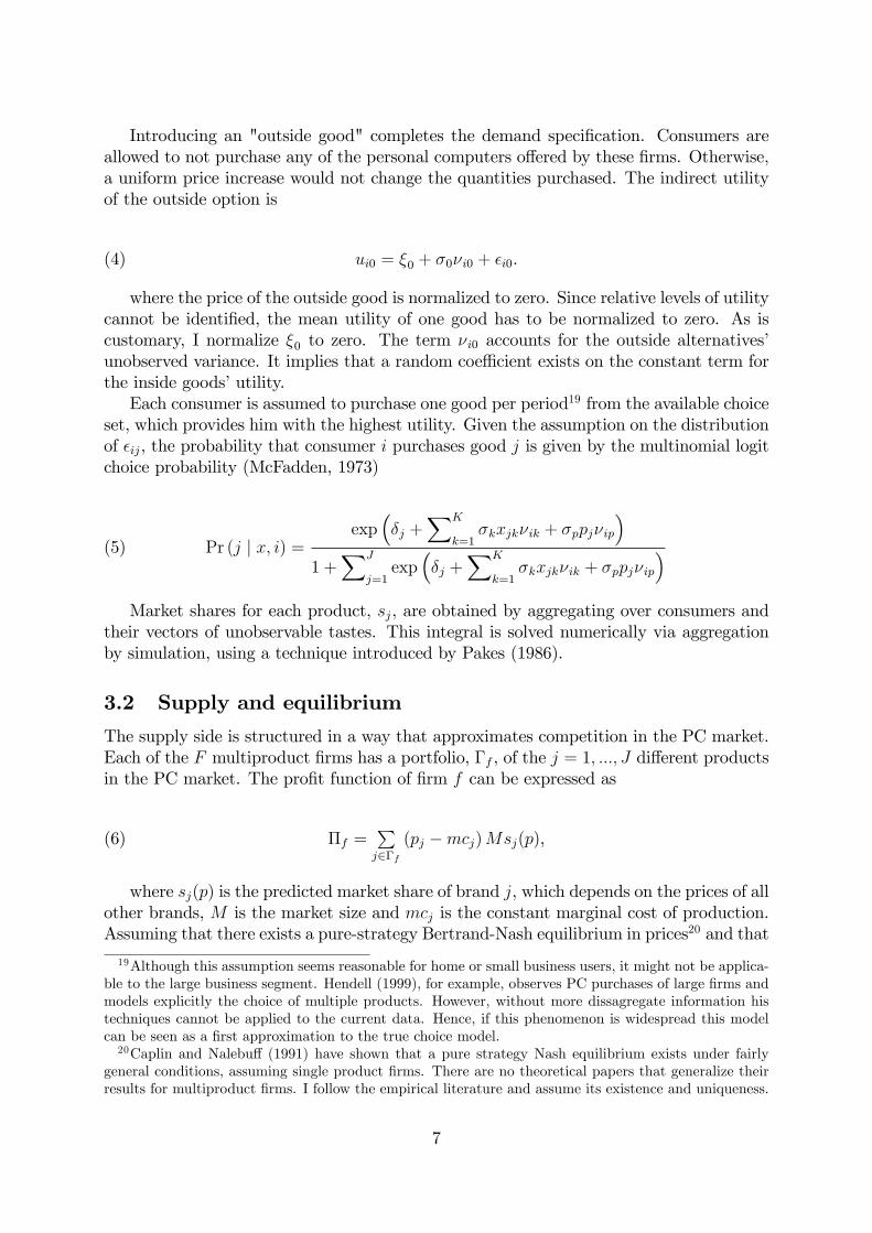
Introducing an "outside good" completes the demand speci�cation. Consumers areallowed to not purchase any of the personal computers o¤ered by these �rms. Otherwise,a uniform price increase would not change the quantities purchased. The indirect utilityof the outside option is

(4) ui0 = �0 + �0�i0 + �i0.

where the price of the outside good is normalized to zero. Since relative levels of utilitycannot be identi�ed, the mean utility of one good has to be normalized to zero. As iscustomary, I normalize �0 to zero. The term �i0 accounts for the outside alternatives�unobserved variance. It implies that a random coe¢ cient exists on the constant term forthe inside goods�utility.Each consumer is assumed to purchase one good per period19 from the available choice

set, which provides him with the highest utility. Given the assumption on the distributionof �ij, the probability that consumer i purchases good j is given by the multinomial logitchoice probability (McFadden, 1973)

(5) Pr (j j x; i) =exp

��j +

XK

k=1�kxjk�ik + �ppj�ip

�1 +

XJ

j=1exp

��j +

XK

k=1�kxjk�ik + �ppj�ip

�Market shares for each product, sj, are obtained by aggregating over consumers and

their vectors of unobservable tastes. This integral is solved numerically via aggregationby simulation, using a technique introduced by Pakes (1986).

3.2 Supply and equilibrium

The supply side is structured in a way that approximates competition in the PC market.Each of the F multiproduct �rms has a portfolio, �f , of the j = 1; :::; J di¤erent productsin the PC market. The pro�t function of �rm f can be expressed as

(6) �f =Pj2�f

(pj �mcj)Msj(p),

where sj(p) is the predicted market share of brand j, which depends on the prices of allother brands, M is the market size and mcj is the constant marginal cost of production.Assuming that there exists a pure-strategy Bertrand-Nash equilibrium in prices20 and that

19Although this assumption seems reasonable for home or small business users, it might not be applica-ble to the large business segment. Hendell (1999), for example, observes PC purchases of large �rms andmodels explicitly the choice of multiple products. However, without more dissagregate information histechniques cannot be applied to the current data. Hence, if this phenomenon is widespread this modelcan be seen as a �rst approximation to the true choice model.20Caplin and Nalebu¤ (1991) have shown that a pure strategy Nash equilibrium exists under fairly

general conditions, assuming single product �rms. There are no theoretical papers that generalize theirresults for multiproduct �rms. I follow the empirical literature and assume its existence and uniqueness.

7

all prices that support it are strictly positive, then the price pj of any product producedby �rm f must satisfy the �rst-order condition

(7) sj(p) +Pr2�f

(pr �mcr)@sr(p)

@pj= 0

This system of J equations can be inverted to solve for the marginal costs. De�neSjr = �@sj(p)=@pr, j; r = 1; :::; J ,

�jr =

�1, if j and r are produced by the same �rm,0, otherwise,

and a J � J matrix with jr = �jr � Sjr. Then, given the product ownershipstructure before the merger (bm), marginal costs (in vector notation) are given by

(8) mc = p� bm(p)�1s(p).

The markup vector in (8) depends only on the parameters of the demand system andthe equilibrium price vector. Therefore, by using the estimated demand parameters wecan compute estimates of price-cost margins and marginal costs without using actualcost information. These calculations are based upon the demand coe¢ cients�consistencyand the equilibrium assumption. For the merger simulation, I use the same equilibriumassumption and the new (after merger) industry structure matrix am. The postmergerequilibrium price vector, p�, solves

(9) p� = cmc+ am(p�)�1s(p�),where cmc are the estimated marginal costs, based on the demand coe¢ cients and the

premerger ownership structure of the industry.The estimated postmerger prices rely on several assumptions: First, the equilibrium

assumption remains the same before and after the merger. While, this needs to be ques-tioned for every possible merger, there are no reasons to doubt its validity for the HP-Compaq merger. Second, the marginal costs and the number of products are held constantat their premerger level. However, this framework allows me to quantify claims that amerger will have cost e¢ ciencies. As a counterfactual exercise, I calculate the necessarycost e¢ ciencies that would leave the postmerger equilibrium prices unchanged and assesstheir plausibility. Third, the postmerger elasticities are calculated based on premergerdata, which implicity assumes that consumer preferences and the outside good�s valueremain constant after the merger. This assumption can be challenged since changes in�rms�strategy within the industry or changes outside the industry could a¤ect both theprice sensitivity and the overall PC demand. Therefore, this analysis is more indicativeof the short rather than the long run response to the merger.

8

3.3 Consumer Welfare

The structural model�s results are also used to calculate consumer welfare changes dueto the merger. I use compensating variation to calculate the dollar amount that wouldleave a consumer indi¤erent before and after the merger. Assuming that the marginalutility of income is �xed, McFadden (1981) and Small and Rosen (1981) show that thecompensating variation of individual i is given by

(10) CVi =lnhXJ

j=0exp

�V amij

�i� ln

hXJ

j=0exp

�V bmij

�i�i

where �i = � + �p�ip is the price coe¢ cient for each individual and V bmij and V amij ,as de�ned in (1), are computed using the premerger prices and postmerger predictedprices, respectively. Aggregating over i and multiplying by the market size gives themean compensating variation. These calculations assume that both the value of the eachproduct�s unobserved characteristic, �j, and the utility from the outside good remainconstant after the merger.

4 Data and Estimation

4.1 Data

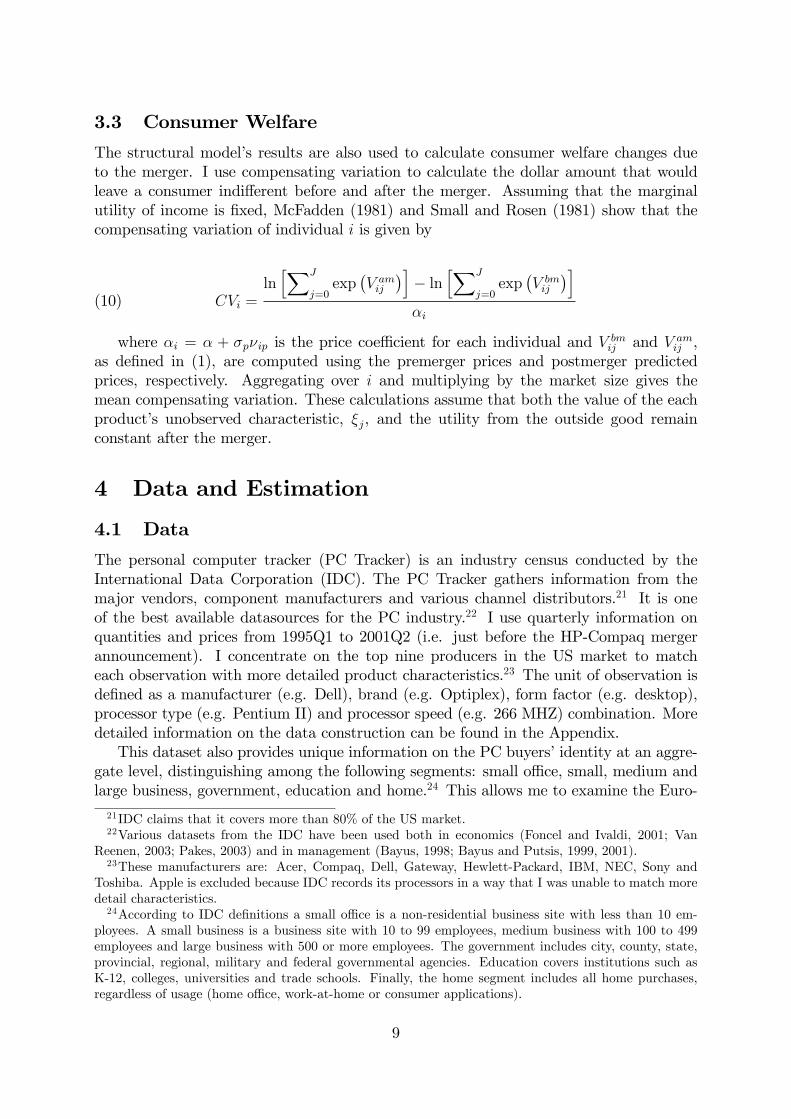
The personal computer tracker (PC Tracker) is an industry census conducted by theInternational Data Corporation (IDC). The PC Tracker gathers information from themajor vendors, component manufacturers and various channel distributors.21 It is oneof the best available datasources for the PC industry.22 I use quarterly information onquantities and prices from 1995Q1 to 2001Q2 (i.e. just before the HP-Compaq mergerannouncement). I concentrate on the top nine producers in the US market to matcheach observation with more detailed product characteristics.23 The unit of observation isde�ned as a manufacturer (e.g. Dell), brand (e.g. Optiplex), form factor (e.g. desktop),processor type (e.g. Pentium II) and processor speed (e.g. 266 MHZ) combination. Moredetailed information on the data construction can be found in the Appendix.This dataset also provides unique information on the PC buyers�identity at an aggre-

gate level, distinguishing among the following segments: small o¢ ce, small, medium andlarge business, government, education and home.24 This allows me to examine the Euro-

21IDC claims that it covers more than 80% of the US market.22Various datasets from the IDC have been used both in economics (Foncel and Ivaldi, 2001; Van

Reenen, 2003; Pakes, 2003) and in management (Bayus, 1998; Bayus and Putsis, 1999, 2001).23These manufacturers are: Acer, Compaq, Dell, Gateway, Hewlett-Packard, IBM, NEC, Sony and

Toshiba. Apple is excluded because IDC records its processors in a way that I was unable to match moredetail characteristics.24According to IDC de�nitions a small o¢ ce is a non-residential business site with less than 10 em-

ployees. A small business is a business site with 10 to 99 employees, medium business with 100 to 499employees and large business with 500 or more employees. The government includes city, county, state,provincial, regional, military and federal governmental agencies. Education covers institutions such asK-12, colleges, universities and trade schools. Finally, the home segment includes all home purchases,regardless of usage (home o¢ ce, work-at-home or consumer applications).

9

pean Competition Commission�s claim that the various customer segments have di¤erentpurchasing patterns and whether the merger would a¤ect certain segments di¤erentially.Hence, in my analysis I estimate the demand model both for the whole market and foreach of the three following segments: home, small business (including the small business,small o¢ ce and medium business segments)25 and large business. These three segmentsaccount for the majority (average 89%) of all PC sales. The largest is the home segment(37%), followed by the small business (34%) and then the large business (17%).26

Despite the large number of small producers, the PC industry is rather concentratedwith the top �ve �rms accounting for 52% and the top ten �rms for 72% of the aggregatesales. Table 1 presents the average percentage shares of the nine �rms included in thesample. They account for 65% of total sales, 60% and 65% for the home and smallbusiness segments respectively, reaching 80% for the large business segment. Tables 2�5provide sales weighted means of the variables used in the speci�cations, both for the overallmarket and di¤erent segments. These variables include quantity (in units of 1,000), price(in $1,000 units), "benchmark" (in units of 1,000), RAM (in units of 100MB), monitorsize and dummies for CD-ROM (1 if standard, 0 otherwise), internet (1 if modem orethernet included as standard, 0 otherwise) and desktop. The variable choice is basedon two criteria: �rst, to capture technological innovation (i.e. the "benchmark" andRAM) and trends in related markets (i.e. the modem/ethernet for internet and CD-ROMfor multimedia). Second, to be relevant both for the overall market and for the threeindividual segments.These tables reveal the remarkable pace of innovation and competition in this industry.

The quantity of products rises from 88 in 1995Q1 to 277 in 2001Q2, along an upwardtrend. The core computer characteristics, "benchmark" and RAM, follow an amazingaverage quarterly growth of 13% and 11% respectively. New components at the startof the sample period, such as the CD-ROM and internet peripherals, that are installedin 68% and 51% of new PCs respectively, di¤use quickly and are virtually standard bythe end of the sample period. Even more spectacularly, this fast technological progressis accompanied by rapidly falling prices. In real terms, the sales-weighted average priceof PCs fell by 45% in the late ninenties.27 This combination of forces allowed portablecomputers to become a¤ordable for more consumers, which can be seen by the negativetrend of the desktop market share. Finally, the tables reveal some interesting di¤erencesamong the various segments. Large businesses, for example, buy more expensive PCs onaverage, with better core characteristics and a stronger preference for portable computers.They are slightly behind, however, in adopting peripherals.

25I calculate aggregate elasticities for each of these segments based on IV logit regressions. Small o¢ ce,small business and medium business have very similar elasticities and for that reason, I combine themin a single segment. I also experimented separating the medium business segment from the combinedsmall o¢ ce-small business segment. Results from either the IV logit or the random coe¢ cients modelcon�rmed their similarity.26I exclude the government and education segments both because of their small market share and

because I could not �nd reliable information regading their market sizes.27There is an extensive empirical literature using hedonic regressions that documents the dramatic

declines in the quality adjusted price of personal computers. See, for example, Dulberger (1989), Gordon(1989), Triplett (1989), Berndt, Griliches and Rappaport (1995) and Pakes (2003).

10

4.2 Estimation

Demand model estimation closely follows Berry (1994) and BLP. The algorithm minimizesa nonlinear GMM function that is the product of instrumental variables and a structuralerror term. This error term is de�ned as the unobserved product characteristics, �j, thatenter the mean utility. In order to compute these unobserved characteristics, I solve forthe mean utility levels, �, by solving the implicit system of equations

(11) s (x; p; �; �2) = S

where s (:) is the vector of calculated market shares and S is the vector of observedmarket shares. This �nds the vector �, given the nonlinear parameters �2, that matchesthe predicted to the observed market shares. Berry (1994) shows that this vector existsand is unique under mild regularity conditions on the distribution of consumer tastes. Itis numerically calculated using BLP�s contraction mapping algorithm. Once this inversionhas been computed, the error term is calculated as �j = �j (x; p; S; �2)� (xj� + �pj).Given a set of instruments, Z = [z1; :::; zM ], a population moment condition can be

written as E[Z 0�(��)] = 0, where �(��) is the above de�ned structural error term evaluatedat the true value parameters. Then, following Hansen (1982), an optimal GMM estimatortakes the form

(12) b� = argmin�

b�(�)0ZA�1Z 0b�(�),where b�(�) is the sample analog to � (�) and A is a consistent estimate of the E [Z 0��0Z].The intuition behind this procedure is straighforward. The structural residuals, de-

�ned above, are the di¤erence between the mean utility and that predicted by the linearparameters, �1 = (�; �). The GMM estimator serves to minimize this di¤erence. Atthe true parameter value ��, the population moment condition is equal to zero, so theestimates would set the sample analog of the moments, i.e. Z 0b�, equal to zero. If thereare more independent moment equations than parameters, the sample analogs can not beset exactly to zero, but as close to zero as possible. By using the inverse of the variance-covariance matrix of the moments, less weight is given to those moments with highervariance. I calculate the weight matrix using the usual two-step procedure, starting withan initial matrix given by Z 0Z. To minimize the GMM function I used both the Nelder-Mead nonderivative search method and the faster Quasi-Newton gradient method basedon an analytic gradient.28

Finally, using the results in Berry, Linton and Pakes (2004), I increased the number ofsimulation draws (more than ten times larger than the average number of products in mysample) to obtain consistent and asymptotically normal estimators for the parameters. I

compute standard errors for the estimates using the asymptotic variance ofpn�b� � ���

given by

(13) (�0�)�1�0

3Xi=1

Vi

!� (�0�)

�1

28For more details see the appendix in Nevo (2000b).

11

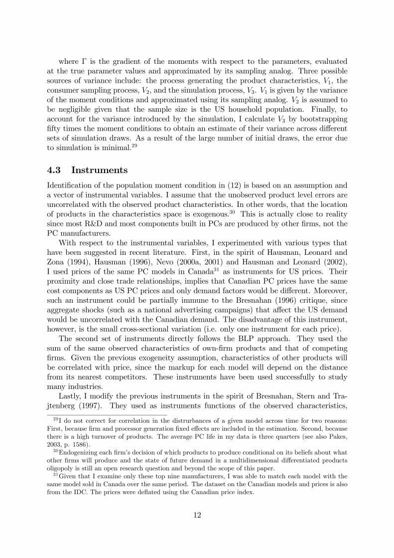
where � is the gradient of the moments with respect to the parameters, evaluatedat the true parameter values and approximated by its sampling analog. Three possiblesources of variance include: the process generating the product characteristics, V1, theconsumer sampling process, V2, and the simulation process, V3. V1 is given by the varianceof the moment conditions and approximated using its sampling analog. V2 is assumed tobe negligible given that the sample size is the US household population. Finally, toaccount for the variance introduced by the simulation, I calculate V3 by bootstrapping�fty times the moment conditions to obtain an estimate of their variance across di¤erentsets of simulation draws. As a result of the large number of initial draws, the error dueto simulation is minimal.29

4.3 Instruments

Identi�cation of the population moment condition in (12) is based on an assumption anda vector of instrumental variables. I assume that the unobserved product level errors areuncorrelated with the observed product characteristics. In other words, that the locationof products in the characteristics space is exogenous.30 This is actually close to realitysince most R&D and most components built in PCs are produced by other �rms, not thePC manufacturers.With respect to the instrumental variables, I experimented with various types that

have been suggested in recent literature. First, in the spirit of Hausman, Leonard andZona (1994), Hausman (1996), Nevo (2000a, 2001) and Hausman and Leonard (2002),I used prices of the same PC models in Canada31 as instruments for US prices. Theirproximity and close trade relationships, implies that Canadian PC prices have the samecost components as US PC prices and only demand factors would be di¤erent. Moreover,such an instrument could be partially immune to the Bresnahan (1996) critique, sinceaggregate shocks (such as a national advertising campaigns) that a¤ect the US demandwould be uncorrelated with the Canadian demand. The disadvantage of this instrument,however, is the small cross-sectional variation (i.e. only one instrument for each price).The second set of instruments directly follows the BLP approach. They used the

sum of the same observed characteristics of own-�rm products and that of competing�rms. Given the previous exogeneity assumption, characteristics of other products willbe correlated with price, since the markup for each model will depend on the distancefrom its nearest competitors. These instruments have been used successfully to studymany industries.Lastly, I modify the previous instruments in the spirit of Bresnahan, Stern and Tra-

jtenberg (1997). They used as instruments functions of the observed characteristics,

29I do not correct for correlation in the distrurbances of a given model across time for two reasons:First, because �rm and processor generation �xed e¤ects are included in the estimation. Second, becausethere is a high turnover of products. The average PC life in my data is three quarters (see also Pakes,2003, p. 1586).30Endogenizing each �rm�s decision of which products to produce conditional on its beliefs about what

other �rms will produce and the state of future demand in a multidimensional di¤erentiated productsoligopoly is still an open research question and beyond the scope of this paper.31Given that I examine only these top nine manufacturers, I was able to match each model with the

same model sold in Canada over the same period. The dataset on the Canadian models and prices is alsofrom the IDC. The prices were de�ated using the Canadian price index.

12

segmented according to their proposed clustering of the PC market during the late eight-ies. My modi�cation is simpler and closer to the competitive enviroment during the latenineties: I calculate the sum of the observed characteristics of products o¤ered by each�rm and its rivals, conditional on the form factor of each computer. The intuition under-lying this modi�cation is that the price of a desktop PC would be more constrained bythe proximity of other desktops rather than a laptop, given their fundamental di¤erencesin functionality and technical characteristics.

5 Results

I turn now on the results from the demand estimation and their implications in termsof markups and pro�t margins. I then assess the robustness of the speci�cation usedto various pertrubations. Next, I simulate the e¤ects of the HP-Compaq merger and asecond, hypothetical, merger between Dell and Compaq. I analyze the mergers�e¤ectsnot only for the whole market, but also for the three customer segments individually. Thechoice of the second merger is intended to demonstrate the variation in the di¤erentialsegment e¤ects.

5.1 Demand Estimates

I use the logit model (i.e. �ij = 0) to examine the importance of instrumenting the priceand test the di¤erent sets of instrumental variables. Table 6 reports the results obtainedfrom regressing ln(Sj) � ln(S0) on prices, characteristics and time �xed e¤ect variables.Columns 1 and 2 report ordinary least squares results. While column 2�s �rm �xed e¤ectsinclusion is an improvement on column 1 (both the price coe¢ cient and the model �tincrease), the majority of products are predicted to have inelastic demands (88.4% forcolumn 1 and 58.4% for column 2). This clearly counters reality.To correct for the price endogeneity, I experiment with di¤erent instrumental variables

in the last �ve columns. In column 3, I use Canadian prices of the same models. Theprice coe¢ cient increases, as expected, but almost a quarter of all the products stillhave inelastic demand. Columns 4 and 5 use the BLP instruments and my modi�edinstruments respectively, in conjuction with Canadian prices. Both the price coe¢ cientand the proportion of inelastic demands remain una¤ected. When I use only the BLPinstruments in column 6, the coe¢ cient on price rises signi�cantly (leaving only 16.45%of products with inelastic demands), but fails to correct for the negative RAM coe¢ cent(implying that, ceteris paribus, consumers prefer lower to higher RAM) and the positivedesktop dummy coe¢ cient (implying that, ceteris paribus, consumers prefer a desktopto a laptop). Moreover, the Hansen-Sargan overidenti�cation test is rejected, suggestingthat the identifying assumptions are not valid.The modi�ed instruments alone seem to control the endogenous prices more e¤ectively,

as seen from the last column. The price coe¢ cient rises further, leaving no products withinelastic demands. Moreover, the test of overidenti�ed restrictions cannot be rejected atthe 1% level of signi�cance, despite the large number of observations. All other coe¢ cientsare statistically signi�cant with their expected signs. The "benchmark" is valued morehighly than RAM and the CD-ROM availability more highly than internet peripherals.

13

The desktop dummy indicates that consumers attach greater value to laptop computers.The only surprising result is the small negative coe¢ cient for monitor size.32 Finally,the processor generation dummies33 indicate that each new CPU generation contributessigni�cantly over the fourth generation, with the sixth generation contributing most. Thisis probably due to the signi�cant improvements to PC hardware and software duringthe sixth generation and the relatively short period since the introduction of the seventhgeneration (the �rst model appears in 2000Q1). Similar results regarding the instrumentalvariable validity hold for each of the three market segments, but for brevity are notreported here.Table 7 reports the random coe¢ cient model results for the whole market. Column 1

replicates column 7 from the previous table to ease comparisons. Due to the di¢ culty ofthe full model estimation and uniqueness of the PC market, a parsimonious list of randomcoe¢ cients has been selected. As Bresnahan, Stern and Trajtenberg (1997) suggested,because of the modularity of personal computers and the ease with which consumers canre-con�gure their machines, not all characteristics carry the same weight. For example,consumers might choose a computer without a modem or CD-ROM as standard, notbecause they do not value it, but because they can buy it later and possibly arbitrage anyprice di¤erences. To the extent that consumers can easily re-con�gure PCs, I would notbe able to capture consumers heterogeneous preferences along these dimensions. Hence,I focus here on random coe¢ cents for the "benchmark" and desktop variables. Theseare essential characteristics for every computer and cannot be altered as easily as othercore characteristics (such as RAM or hard disk) or peripherals (such as the modem orCD-ROM).Full model results are in column 2. The random coe¢ cients are identi�ed by observing

multiple markets with di¤erent distributions of the observed characteristics. Although thesample period is short (only six and a half years), the pace of the PC industry�s evolutionprovides con�dence that I can identify these parameters. For the whole market, threeout of four coe¢ cients have Z-statistics greater than one. For the segment estimations(Table 10 ), this is eight out of twelve. Moreover, each characteristic is estimated tohave a signi�cantly positive e¤ect either on the mean or standard deviation of the tastedistribution, with the constant the only exception. The magnitudes of the standarddeviations relative to their means suggest that there is signi�cant heterogeneity on priceand on the preferences for desktop computers. Most of the remaining coe¢ cients retaintheir signs and signi�cance, as in the IV regressions.The advantage of using the random coe¢ cients model stems from the more realistic

substitution patterns among PCs, which is important for the merger simulation. A smallsample of those elasticities is given in Table 8. In the top panel I present �ve models mar-keted by Acer in the �rst quarter of 1995 along with their main characteristics. Markups(in the last column) rise almost monotonically with price. This is in contrast to the logit

32This most likely stems from the introduction of more advanced and thinner monitors of the same sizein the last 2-3 years of the data. These are not recorded separately.33In dynamic markets with frequent changes in the processor�s underlying technology, such as the PC

market, competition among products of the same CPU generation di¤ers signi�cantly from competitionwith products of other generations. Applications of this idea in a standard hedonic framework can befound in Pakes (2003) and Chwelos, Berndt and Cockburn (2004), where they use indicator variables forCPU generations to estimate "piece-wise" stable coe¢ cients for the PC characteristics.

14

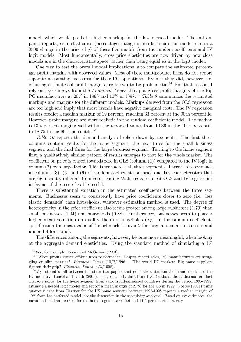
model, which would predict a higher markup for the lower priced model. The bottompanel reports, semi-elasticities (percentage change in market share for model i from a$500 change in the price of j) of these �ve models from the random coe¢ cents and IVlogit models. Most fundamentally, cross price elasticities are now driven by how closemodels are in the characteristics space, rather than being equal as in the logit model.One way to test the overall model implications is to compare the estimated percent-

age pro�t margins with observed values. Most of these multiproduct �rms do not reportseparate accounting measures for their PC operations. Even if they did, however, ac-counting estimates of pro�t margins are known to be problematic.34 For that reason, Irely on two surveys from the Financial Times that put gross pro�t margins of the topPC manufacturers at 20% in 1996 and 10% in 1998.35 Table 9 summarizes the estimatedmarkups and margins for the di¤erent models. Markups derived from the OLS regressionare too high and imply that most brands have negative marginal costs. The IV regressionresults predict a median markup of 19 percent, reaching 33 percent at the 90th percentile.However, pro�t margins are more realistic in the random coe¢ cients model. The medianis 13.4 percent ranging well within the reported values from 10.36 in the 10th percentileto 18.75 in the 90th percentile.36

Table 10 reports the demand analysis broken down by segments. The �rst threecolumns contain results for the home segment, the next three for the small businesssegment and the �nal three for the large business segment. Turning to the home segment�rst, a qualitatively similar pattern of results emerges to that for the whole market. Thecoe¢ cient on price is biased towards zero in OLS (column (1)) compared to the IV logit incolumn (2) by a large factor. This is true across all three segments. There is also evidencein columns (3), (6) and (9) of random coe¢ cients on price and key characteristics thatare signi�cantly di¤erent from zero, leading Wald tests to reject OLS and IV regressionsin favour of the more �exible model.There is substantial variation in the estimated coe¢ cients between the three seg-

ments. Businesses seem to consistently have price coe¢ cients closer to zero (i.e. lesselastic demands) than households, whatever estimation method is used. The degree ofheterogeneity in the price coe¢ cient also seems greater among large businesses (1.79) thansmall businesses (1.04) and households (0.88). Furthermore, businesses seem to place ahigher mean valuation on quality than do households (e.g. in the random coe¢ cientsspeci�cation the mean value of "benchmark" is over 2 for large and small businesses andunder 1.4 for home).The di¤erences among the segments, however, become more meaningful, when looking

at the aggregate demand elasticities. Using the standard method of simulating a 1%

34See, for example, Fisher and McGowan (1983).35"When pro�ts switch o¤-line from performance: Despite record sales, PC manufacturers are strug-

gling on slim margins", Financial Times (10/2/1996). "The world PC market: Big name supplierstighten their grip", Financial Times (4/3/1998).36My estimates fall between the other two papers that estimate a structural demand model for the

PC industry. Foncel and Ivaldi (2001), using quarterly data from IDC (without the additional productcharacteristics) for the home segment from various industrialized countries during the period 1995-1999,estimate a nested logit model and report a mean margin of 2.7% for the US in 1999. Goeree (2004) usingquarterly data from Gartner for the US home segment between 1996-1998 reports a median margin of19% from her preferred model (see the discussion in the sensitivity analysis). Based on my estimates, themean and median margins for the home segment are 12.6 and 11.5 percent respectively.

15

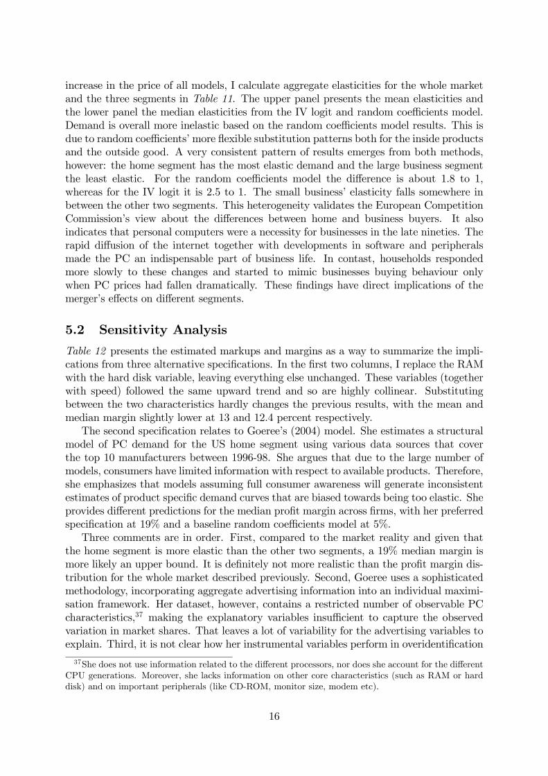
increase in the price of all models, I calculate aggregate elasticities for the whole marketand the three segments in Table 11. The upper panel presents the mean elasticities andthe lower panel the median elasticities from the IV logit and random coe¢ cients model.Demand is overall more inelastic based on the random coe¢ cients model results. This isdue to random coe¢ cients�more �exible substitution patterns both for the inside productsand the outside good. A very consistent pattern of results emerges from both methods,however: the home segment has the most elastic demand and the large business segmentthe least elastic. For the random coe¢ cients model the di¤erence is about 1.8 to 1,whereas for the IV logit it is 2.5 to 1. The small business�elasticity falls somewhere inbetween the other two segments. This heterogeneity validates the European CompetitionCommission�s view about the di¤erences between home and business buyers. It alsoindicates that personal computers were a necessity for businesses in the late nineties. Therapid di¤usion of the internet together with developments in software and peripheralsmade the PC an indispensable part of business life. In contast, households respondedmore slowly to these changes and started to mimic businesses buying behaviour onlywhen PC prices had fallen dramatically. These �ndings have direct implications of themerger�s e¤ects on di¤erent segments.

5.2 Sensitivity Analysis

Table 12 presents the estimated markups and margins as a way to summarize the impli-cations from three alternative speci�cations. In the �rst two columns, I replace the RAMwith the hard disk variable, leaving everything else unchanged. These variables (togetherwith speed) followed the same upward trend and so are highly collinear. Substitutingbetween the two characteristics hardly changes the previous results, with the mean andmedian margin slightly lower at 13 and 12.4 percent respectively.The second speci�cation relates to Goeree�s (2004) model. She estimates a structural

model of PC demand for the US home segment using various data sources that coverthe top 10 manufacturers between 1996-98. She argues that due to the large number ofmodels, consumers have limited information with respect to available products. Therefore,she emphasizes that models assuming full consumer awareness will generate inconsistentestimates of product speci�c demand curves that are biased towards being too elastic. Sheprovides di¤erent predictions for the median pro�t margin across �rms, with her preferredspeci�cation at 19% and a baseline random coe¢ cients model at 5%.Three comments are in order. First, compared to the market reality and given that

the home segment is more elastic than the other two segments, a 19% median margin ismore likely an upper bound. It is de�nitely not more realistic than the pro�t margin dis-tribution for the whole market described previously. Second, Goeree uses a sophisticatedmethodology, incorporating aggregate advertising information into an individual maximi-sation framework. Her dataset, however, contains a restricted number of observable PCcharacteristics,37 making the explanatory variables insu¢ cient to capture the observedvariation in market shares. That leaves a lot of variability for the advertising variables toexplain. Third, it is not clear how her instrumental variables perform in overidenti�cation

37She does not use information related to the di¤erent processors, nor does she account for the di¤erentCPU generations. Moreover, she lacks information on other core characteristics (such as RAM or harddisk) and on important peripherals (like CD-ROM, monitor size, modem etc).

16

tests and how they change in each model speci�cation.I lack the advertising data to test for Goeree�s "limited information" story. Columns

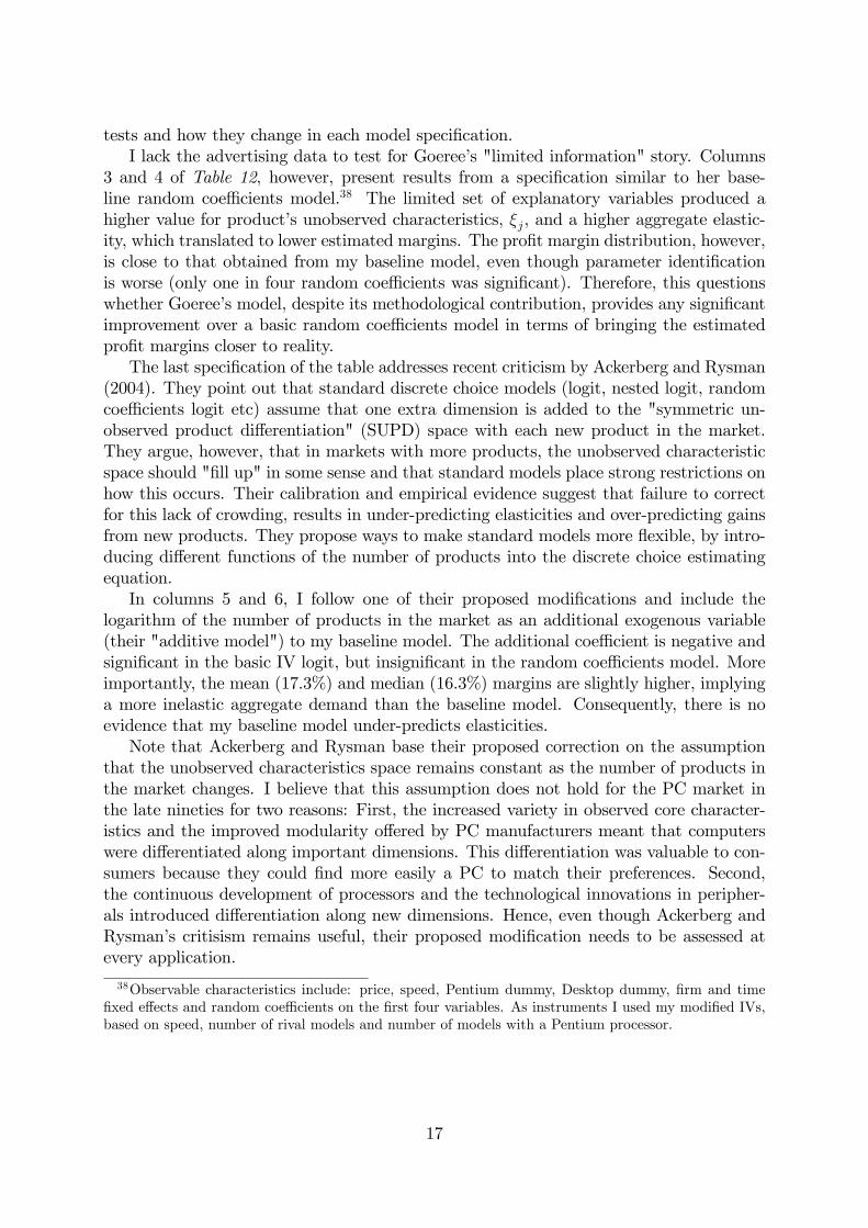
3 and 4 of Table 12, however, present results from a speci�cation similar to her base-line random coe¢ cients model.38 The limited set of explanatory variables produced ahigher value for product�s unobserved characteristics, �j, and a higher aggregate elastic-ity, which translated to lower estimated margins. The pro�t margin distribution, however,is close to that obtained from my baseline model, even though parameter identi�cationis worse (only one in four random coe¢ cients was signi�cant). Therefore, this questionswhether Goeree�s model, despite its methodological contribution, provides any signi�cantimprovement over a basic random coe¢ cients model in terms of bringing the estimatedpro�t margins closer to reality.The last speci�cation of the table addresses recent criticism by Ackerberg and Rysman

(2004). They point out that standard discrete choice models (logit, nested logit, randomcoe¢ cients logit etc) assume that one extra dimension is added to the "symmetric un-observed product di¤erentiation" (SUPD) space with each new product in the market.They argue, however, that in markets with more products, the unobserved characteristicspace should "�ll up" in some sense and that standard models place strong restrictions onhow this occurs. Their calibration and empirical evidence suggest that failure to correctfor this lack of crowding, results in under-predicting elasticities and over-predicting gainsfrom new products. They propose ways to make standard models more �exible, by intro-ducing di¤erent functions of the number of products into the discrete choice estimatingequation.In columns 5 and 6, I follow one of their proposed modi�cations and include the

logarithm of the number of products in the market as an additional exogenous variable(their "additive model") to my baseline model. The additional coe¢ cient is negative andsigni�cant in the basic IV logit, but insigni�cant in the random coe¢ cients model. Moreimportantly, the mean (17.3%) and median (16.3%) margins are slightly higher, implyinga more inelastic aggregate demand than the baseline model. Consequently, there is noevidence that my baseline model under-predicts elasticities.Note that Ackerberg and Rysman base their proposed correction on the assumption

that the unobserved characteristics space remains constant as the number of products inthe market changes. I believe that this assumption does not hold for the PC market inthe late nineties for two reasons: First, the increased variety in observed core character-istics and the improved modularity o¤ered by PC manufacturers meant that computerswere di¤erentiated along important dimensions. This di¤erentiation was valuable to con-sumers because they could �nd more easily a PC to match their preferences. Second,the continuous development of processors and the technological innovations in peripher-als introduced di¤erentiation along new dimensions. Hence, even though Ackerberg andRysman�s critisism remains useful, their proposed modi�cation needs to be assessed atevery application.

38Observable characteristics include: price, speed, Pentium dummy, Desktop dummy, �rm and time�xed e¤ects and random coe¢ cients on the �rst four variables. As instruments I used my modi�ed IVs,based on speed, number of rival models and number of models with a Pentium processor.

17

5.3 Merger Analysis

Using the structural demand parameters and the estimated marginal costs, I simulate thepostmerger equilibrium for the whole PC market. The upper panel of Table 13 presentsprice and quantity changes39 both for the merger between HP and Compaq and the hy-pothetical merger between Dell and Compaq, at three di¤erent periods. In line withtheoretical research on unilateral e¤ects, both mergers result in higher prices for all prod-ucts in the market, smaller sales for the merging entity and larger sales for the non-merging�rms. Note also that any merger would raise prices more in 2001 than in 1998 or 1995.In the HP-Compaq case, for example, the mean percentage price increase would be 0.58in the �rst period, 1.00 in the second and 1.11 in the third. The same e¤ect across timeis also true for the hypothetical merger between Dell and Compaq, with overall higherinduced mean price increases, reaching 1.87 percent in 2001.The e¤ect of a merger on prices is a combination of the relevant strategic position of

the �rms involved (portfolio of products, degree of di¤erentiation and market power) andthe aggregate demand elasticity. The impact on prices is higher in the second merger,because the joint market power of Dell and Compaq is higher than that of HP andCompaq at any point in time. Both mergers, however, raise prices more in 2001 than in1995, because aggregate PC demand had become more inelastic. During the last decade,the personal computer developed from an awkward and unfriendly tool for specialists intoan indispensable part of every day life. The HP-Compaq merger would have caused lessconcern, in terms of its e¤ect on competition and consumer welfare, at the begginingrather than at the end of the sample. Therefore, examining the di¤erential e¤ects of amerger at various points in time, provides competition authorities with a sense of themarket dynamics that can be useful for any merger evaluation.The equilibrium price and quantity changes assume that (marginal) cost conditions

remain the same before and after the merger. However, �rms often advocate, both totheir shareholders and competition authorities, that cost e¢ ciencies can be achieved afterthe merger. Since it is di¢ cult to predict the actual cost reductions, the lower panel ofTable 13 presents statistics on the following counterfactual: what would be the necessarycost reductions such that the merger would have no e¤ect on prices? For the HP-Compaqmerger in 2001, for example, the average required cost e¢ ciency is 1.5 percent with themaximum being 6.3 percent. Both are realistic. In fact, Ms C. Fiorina, the CEO of HP,targeted an overall 5-7 percent cost reduction.40

The hypothetical merger between Dell and Compaq in 2001 would need a much higherlevel of cost savings (2.5 percent on average, with a maximum of 10.3). The emerging pic-ture is similar: larger cost decreases would be required over time to o¤set any postmergerprice increases. These results are complementary to those on prices and quantities andprovide another perspective on which a merger can be assessed.The price and quantity results, although indicative, do not provide any criteria on

39It is worth noting, as Berry and Pakes (1993) mention, that the random coe¢ cient model is �exibleenough that even though a price setting behavior is assumed, pairs of prices are allowed to act as strategiccomplements or as strategic substitutes. In other words, what I �nd is that when a merger raises theprices of the merging �rms, prices of the rivals went either way (although the majority of them, and hencethe mean and median, were positive).40"HP lays the ground for $3bn savings", Financial Times (5/6/2002). "HP to hit cost cuts target a

year early", Financial Times (4/12/2002).

18

which to judge the magnitude of these e¤ects. A structural model, however, can translatethese price movements into consumer welfare changes. Table 14 provides changes inthe consumer surplus, �rm�s revenues and pro�ts as a result of the various mergers.Still focusing on 2001, two results regarding the HP-Compaq merger stand out: First,the merger raises their combined pro�tability ($1.86 million), despite a fall in revenues.Second, the companies that bene�t most are Dell (with a $6.15 million increase in pro�ts),Gateway ($2.00 million) and IBM ($1.42 million). That matches reality well, where themerger�s critics, such as Mr. Hewlett, insisted that competitors like IBM and Dell standto gain the most from the merger: "HP�s rivals raised almost no objections to the merger.We are not surprised. We believe Dell, Sun and IBM must be delighted at the prospect ofa merger...".41 These results provide a clear explanation as to why the major competitorsdid not complain about the merger: if the merged companies were to raise prices, these�rms would bene�t the most from such a strategy.According to the estimates, the 2001 HP-Compaq merger would result in a $1.06

million loss in consumer surplus, but on a positive $11.67 million overall welfare gain.These results are empirical support for the merger approval by both the US FederalTrade Commission and the European Competition Commission. Sti¤ price competitionand the high degree of substitutability among PC manufacturers meant that the mergedentity�s market power was not a signi�cant threat to competition. Finally, in line withthe previous results, a merger between Dell and Compaq would have been more harmfulto consumer welfare at any point in time.Using the predicted postmerger prices for the whole market and the estimated demand

parameters for each sector, I calculate the merger e¤ects on each segment separately. Table15 summarizes the predicted percentage changes in prices and quantities for the threesegments. Due to di¤erences in the underlying demand, the most striking phenomenon isthe wide variation on quantity responces among segments. For example, a similar increasein prices from a 1995 merger between HP and Compaq (average percentage increase 0.61for home, 0.58 for small and 0.55 for large), would have resulted in average percentagequantity decreases of 7.26 for home, 4.61 for small business and 2.53 for large business.The same is true for the Dell-Compaq merger, with ampli�ed results. To a large extentthis phenomenon persists over time, indicating the heterogeneity in preferences amongthe three sectors.This price and quantity variation becomes more meaningful, when looking at the

predicted changes in consumer surplus and �rms�variable pro�ts. Tables 16, 17 and 18present these results for the home, small business and large business segments respectively.The value of this cross-sectional analysis can be seen most clearly in the HP-Compaqmerger in 2001. Although results from the whole market indicated that the combined�rm�s pro�tability would be positive, segment examination draws a more detailed picture:the merger would be unpro�table for the home (-$0.5 million) and the small business(-$0.26 million) segments, with all of the gains coming from the large business segment($1.80 million). This supports the view that the merger was a "defensive move"42 targeteddirectly at the large business segment,43 rather than an attempt to monopolise the PC

41"Titanic failures", Red Herring (8/5/2002).42"The HP-Compaq deal, which would consolidate the world�s second and third largest PC makers, is

thus best seen as a defensive move in a shrinking industry" The Economist (29/9/2001).43"Fiorina (CEO of HP) and other HP executives insist that they must sell PCs to compete for lucra-

19

market. Hence, from the �rm�s point of view, this cross-sectional analysis provides a morecomprehensive picture of the strengths and weaknesses of a possible merger.Segment analysis is also valuable from a public policy perspective. Consumer loss

from the HP-Compaq merger in 2001, for example, is much higher for the home segmentthan for the other segments. This is not the case for all mergers across time. In thehypothetical Dell-Compaq merger in 1998, the large Business segment has a negativeconsumer surplus, which is larger than that of the other two segments. Total welfare(consumer plus producer pro�ts), however, is signi�cantly smaller in the home than inthe small or large business sectors. Given the size of the PC industry, these e¤ects acrosssegments would probably not change antitrust authorities�overall decision regarding theHP-Compaq merger. In merger cases, however, where households are believed to bemore vulnerable than business buyers, knowledge of these di¤erential e¤ects can provideregulators with valuable information on overall merger assessment.

6 Conclusion

Evaluating the e¤ects of a proposed merger has taken centre stage in debates on com-petition policy. This paper contributes to this debate by examining how information onthe purchasing patterns of di¤erent customer segments can be used to more accuratelyevaluate the economic impact of mergers. Using a detailed dataset that covers the lead-ing PC manufacturers in the US during the late nineties, I evaluate the welfare e¤ects ofthe largest merger in the history of the PC industry, that between Hewlett-Packard andCompaq, along with a second hypothetical merger. I use a �exible structural model toestimate demand both for the whole market and for each of the three segments (home,small business and large business). The postmerger oligopolistic equilibrium is then sim-ulated under various assumptions. The di¤erential welfare implications of these mergersare computed both across time and across segments.Results from the demand estimation and merger analysis reveal that: (i) the random

coe¢ cients model provides a more realistic picture of the market than simpler mod-els. This advances our knowledge for the performance of these models in di¤erentiatedoligopolistic markets with a large number of products. (ii) the demand speci�cation isfound to be robust to various perturbations. This sample counters recent criticisms that arandom coe¢ cient model either over-estimates (Goeree, 2004) or under-estimates (Acker-berg and Rysman, 2004) elasticities. (iii) despite being the world�s second and thirdlargest PC manufacturers, the merged HP-Compaq entity would not raise postmergerprices signi�cantly in 2001. Ease of entry, strong price competition and the high degreeof substitutability among PCs meant that the merged entity�s market power was not sig-ni�cant to threaten competition. (iv) there is considerable heterogeneity in preferencesacross segments that persists over time, and (v) the merger e¤ects vary signi�cantly acrosssegments.Although consumer groups with di¤erent purchasing patterns have been recognised

in other industries as well, this is the �rst study to systematically integrate them into

tive corporate customers" (The Boston Globe, 9/7/2003). Although personal computers provided lowermargins, they were perceived as a complimentary good to other products (such as servers or printers)and thus formed an integral part of HP�s strategy to compete for large business customers.

20

a merger analysis. Analysing the di¤erential merger e¤ects by segments has importantimplications for both �rms and competition authorities. In the HP-Compaq case, forexample, an attempt from the merged entity to take advantage of its full product linewould result in negative pro�ts in the home and small business segments, with morethan compensating gains from the large business segment. Hence, this analysis provides�rms with a more accurate picture of the merger, which can also be used for strategicpurposes. For example, �rms can alter their product portfolio after the merger to matchthe segments� preferences more closely. The HP-Compaq evaluation also reveals thatthe merger would harm home consumers more than business buyers. The magnitudeof consumer losses in this particular case would probably not change regulators�overalldecision. In mergers, however, where the welfare impact is stronger and households arebelieved to be more vulnerable than businesses, knowledge of these di¤erential e¤ectsbecomes very important for antitrust authorities. More research is required to examineconsumer segment heterogeneity and its consequences in other industries as well.Future research also needs to address other dimensions related to postmerger equilib-

rium. Firms can a¤ect postmerger competition using a variety of non-price strategies,such as advertising, R&D, new product development and brand life cycles. In addition,a merger can trigger �rm entry or exit decisions that can counterbalance changes in con-centration. The empirical method used in this paper is not suitable to incorporate suchdecisions. The dynamic framework of �rm behavior developed by Ericson and Pakes(1995) and its applications on mergers (Gowrisankaran and Town, 1997; Gowrisankaran,1999) provides a basis to incorporate such dimensions and is promising for future research.

7 Appendix - Data Construction

Quarterly data on quantities and prices44 between 1995Q1 and 2001Q2 was taken fromthe PC Tracker census conducted by the International Data Corporation�s (IDC). Theavailable dataset provided disaggregation by manufacturer, brand name, form factor,45

chip type (e.g. 5th Generation) and processor speed bandwidth (e.g. 200-300 MHz).However, during the late nineties, there was a surge in the number and variety of newprocessors, with Intel trying to achieve greater market segmentation by selling a broaderrange of vertically di¤erentiated processors. In addition, the internet and the proliferationof multimedia meant that PCs were di¤erentiated in a variety of dimensions that wouldbe essential to control for. For that purpose, I concentrated on the top nine manufacturersin the US market (i.e. those who represented the majority of sales and for whom reliableadditional information could be collected).Each observation in the IDC dataset was matched with more detailed product charac-

teristics from various PC magazines.46 To be consistent with the IDC de�nition of price,

44Prices are de�ned by the IDC as "the average end-user (street) price paid for a typical systemcon�gured with chassis, motherboard, memory, storage, video display and any other components thatare part of an "average" con�guration for the speci�c model, vendor, channel or segment". Prices werede�ated using the Consumer Price Index from the Bureau of Labor Statistics.45Form factor means whether the PC is a desktop, notebook or ultra portable. The last two categories

were merged into one.46The characteristics data was taken from PC magazines (PC Magazine, PC Week, PC World, Com-

puter Retail Week, Byte.com, Computer User, NetworkWorld, Computer World, Computer Reseller

21

I assign the characteristics of the median model per IDC observation if more than twomodels were available. The justi�cation for this choice is that I preferred to keep the IDCtransaction prices, rather than substitute them with the list prices published in the maga-zines. An alternative approach followed by Pakes (2003) would be to list all the availableproducts by IDC observation with their prices taken from the magazines and their salescomputed by splitting the IDC quantity equally among the observations. While, bothapproaches adopt ad hoc assumptions, qualitatively the results would be the same. Bothlist and transaction prices experienced a dramatic fall over this period and the increasein the number and variety of PCs o¤ered would have been even more ampli�ed with thelatter approach. Finally, instead of using the seventeen processor type dummies and thespeed of each chip as separate characteristics, I merge them using CPU "benchmarks"for each computer. Hence, my �nal unit of observation is de�ned as a manufacturer (e.g.Dell), brand (e.g. Optiplex), form factor (e.g. desktop), processor type (e.g. PentiumII), processor speed (e.g. 266 MHZ) combination with additional information on othercharacteristics such as the RAM, hard disk, modem/ethernet, CD-ROM and monitor size.The potential market size for the home segment is assumed to be the number of US

households (taken from the Current Population Survey). The small and large businessmarket sizes are the total number of employees as reported respectivelly in the Statisticsof US Businesses. I performed various robustness checks by reducing the market sizes orby �tting di¤erent di¤usion curves (not reported here). The results do not change in anyfundamental way.

8 References

Ackerberg, D. and Rysman, M. (2004) "Unobserved Product Di¤erentiation in DiscreteChoice Models: Estimating Price Elasticities and Welfare E¤ects", RAND Journal ofEconomics, forthcoming.Andrade, G., Mitchell, M. and Sta¤ord, E. (2001) "New Evideance and Perspectives

on Mergers", Journal of Economic Pespectives, 15, 103-120.Baker, J. P. and Bresnahan, T. (1985) "The Gains from Merger or Collusion in

Product-Di¤erentiated Industries", Journal of Industrial Economics, 33, 427-444.Bajari, P. and Benkard, C. (2004) "Demand Estimation with Heterogeneous Con-

sumers and Unobserved Product Characteristics: A Hedonic Approach", mimeo, Dept.of Economics, Stanford University.Bayus, B. L. (1998) "An Analysis of Product Lifetimes in a Technologically Dynamic

Industry", Management Science, 44 (June), 763-775.Bayus, B. L. and Putsis, W. (1999) "Product Proliferation: An Empirical Analysis of

Product Line Determinants and Market Outcomes", Marketing Science, 18 (2), 137-153.Bayus, B. L. and Putsis, W. (2001) "An Empirical Analysis of Firm Product Line

Decisions", Journal of Marketing Research, 38 (February), 110-118.Berry, S. (1994) "Estimating Discrete-Choice Models of Product di¤erentiation",RAND

Journal of Economics, 25, 242-262.Berry, S., Carnall, M. and Spiller, P. (1997) "Airline Hubs: Costs, Markups and the

Implications of Customer Heterogeneity", mimeo, Yale Economics Department.

News, InfoWorld, Edge: Work-Group Computing Report, Computer Shopper) and Datasources.

22

Berry, S. and Pakes, A. (1993) "Some Applications and Limitations of Recent Advancesin Empirical Industrial Oranization: Merger Analysis", American Economic Review, 83,247-252.Berry, S. and Pakes, A. (2002) "The Pure Characteristics Demand Model", mimeo,

Harvard University.Berry, S., Levinson, J., and Pakes, A. (1995) "Automobile Prices in Market Equilib-

rium", Econometrica, 63, 841-90.Berry, S., Linton, O., and Pakes, A. (2004) "Limit Theorems for Estimating the Para-

meters of Di¤erentiated Product Demand Systems", Review of Economic Studies, 71(3),613-654.Berndt, E., Griliches, Z. and Rappaport, N. (1995) "Econometric estimates of price

indexes for personal computers in the 1990�s", Journal of Econometrics, 68, 243-268.Boyd, J. and Mellman, K. (1980) "The E¤ect of Fuel Economy Standards on the

US Automotive Market: A Hedonic Demand Analysis", Transportantion Research, 14A,367-378.Bresnahan, T. (1996) "Comment: Valuation of New Goods Under Perfect and Im-

perfect Competition", In T. F. Bresnahan and R. Gordon, eds., The Economics of NewGoods. Chicago: National Bureau of Economic Research.Bresnahan, T. and Greenstein, S. (1999) "Technological Competition and the Struc-

ture of the Personal Computer Industry", Journal of Industrial Economics, 47, 1-40.Bresnahan, T., Stern, S. and Trajtenberg, M. (1997) "Market Segmentation and the

Sources of Rents from Innovation: Personal Computers in the late 1980s", RAND Journalof Economics, 28, S17-S44.Cardell, N. and Dunbar, F. (1980) "Measuring the Societal Impacts of Automobile

Downsizing", Transportation Research, 14A, 423-434.Caplin, A. and Nalebubu¤, B. (1991) "Aggregation and Imperfect Competition: On

the Existence of Equilibrium", Econometrica, 59, 25-59.Chwelos, P., Berndt, E. and Cockburn, I. (2004) "Faster, Smaller, Cheaper: An He-

donic Price Analysis of PDAs", Working Paper 10746, NBER.Davis, P. (2000) "Empirical Models of Demand for Di¤erentiated Products", European

Economic Review, 44, 993-1005.Deaton, A. and Muellbauer, J. (1980) "An Almost Ideal Demand System", American

Economic Review, 70, 312-326.Dube, J. P. (2004) "Product Di¤erentiation and Mergers in the Carbonated Soft Drink

Industry", mimeo, University of Chicago Graduate School of Business.Dulberger, E. (1989) "The Application of an Hedonic Model to a Quality Adjusted

Price Index for Computer Processors", in Jorgenson and Landau eds., Technology andCapital Formation, MIT Press.Ericson, R and Pakes, A. (1995) "An Alternative Theory of Firm and Industry Dy-

namics", Review of Economic Studies, 62, 53-82.Fisher, F. M. and McGowan, J. J. (1983) "On the Misuse of Accounting Rates of

Return to Infer Monopoly Pro�ts", American Economic Review, 73, 82-97.Foncel, J. and Ivaldi, M. (2001) "Operating System Prices in the Home PC Market",

mimeo, University of Toulouse.Genakos, C. (2004) "Product Life Cycles in the Personal Computer Industry", mimeo,

Economics Department, London Business School.

23

Genakos, C., Kühn, K. and Van Reenen, J. (2004) "The Incentives of a Monopolist toDegrade Interoperability: Theory and Evidence from the Personal Computer and ServerMarket", mimeo, London School of Economics, Centre for Economic Performance.Goeree, A. S. (2004) "Advertising in the US Pesonal Computer Industry", mimeo,

Faculty of Economics and Econometrics, University of Amsterdam.Goolsbee, A. and Petrin, A. (2004) "The Consumer Gains from Direct Broadcast

Satellites and the Competition with Cable TV," Econometrica, 72(2), 351-381.Gordon, R. (1989) "The Postwar Evolution of Computer Prices", in Jorgenson and

Landau eds., Technology and Capital Formation, MIT Press.Gowrisankaran, G. (1999) "A Dynamic Model of Endogenous Horizontal Mergers,"

RAND Journal of Economics, 30, 56 �83.Gowrisankaran, G. and Town, R. J. (1997) "Dynamic Equilibrium in the Hospital

Industry." Journal of Economics and Management Strategy, 6, 45�74.Hansen, L. (1982) "Large Sample Properties of Generalized Method of Moments Es-

timators", Econometrica, 50, 1029-1054.Hausman, J. A., Leonard, G. and Zona, J. D. (1994) "Competitive Analysis with

Di¤erentiated Products", Annales D�Economie at de statistique, 34, 159-180.Hausman, J. A. and Leonard, G. (2002) "The Competitive E¤ects of a New Product

Introduction: A Case Study", The Journal of Industrial Economics, 3, 235-261.Hausman, J. A. (1996) "Valuation of New Goods Under Perfect and Imperfect Compe-

tition", In T. F. Bresnahan and R. Gordon, eds., The Economics of New Goods. Chicago:National Bureau of Economic Research.Hendel, I. (1999) "Estimating Multiple Discrete-Choice Models: An Application to

Computerization Returns", Review of Economic Studies, 66, 423-446.Ivaldi, M., Jullien, B., Rey, P., Seabright, P. and Tirole, J. (2003) "The Economics of

Unilateral E¤ects", Interim Report for DG Competition, European Commission.Ivaldi, M. and Verboven, F. (2004) "Quantifying the E¤ects from Horizontal Merg-

ers in European Competition Policy", International Journal of Industrial Organization,forthcoming.Lancaster, J. (1971) Consumer Demand: A New Approach. New York: Columbia

University Press.Langlois, R. (1992) "External Economies and Ecomic Progress: The Case of the Mi-

crocomputer Industry", Business History Review, 66, 1-60.McFadden, D. (1973) "Conditional Logit Analysis of Qualitative Choice Behavior", in

P. Zarembka, eds., Frontiers of Econometrics, New York, Academic Press.McFadden, D. (1981) "Econometric Models of Probabilistic Choice", in C.F. Manski

and D. McFadden, eds., Structural Analysis of Discrete Data, MAss.: MIT Press.McFadden, D. and Train, K. (2000) "Mixed MNL models for discrete response", Jour-

nal of Applied Econometrics, 15, 447-470.Nevo, A. (2000a) "Mergers with Di¤erentiated Products: The Case of the Ready-to-

eat Cereal Industry", RAND Journal of Economics, 31 (3), 395-421.Nevo, A. (2000b) "A Practitioner�s Guide to Estimation of Random Coe¢ cients Logit

Models of Demand", Journal of Economics & Management Strategy, 9(4), 513-548.Nevo, A. (2001) "Measuring Market Power in the Ready-to-Eat Cereal Industry",

Econometrica, 69, 307-342.

24

Pakes, A. (1986) "Patents as Options: Some Estimates of the Value of Holding Euro-pean patent Stocks", Econometrica, 54, 755-84.Pakes, A. (2003) "A Reconsideration of Hedonic Price Indices with an Application to

PC�s", American Economic Review, 93 (5), 1578-1596.Peters, C. (2001) "Evaluating the Performance of Merger Simulation: Evidence from

the US Airline Industry", mimeo, Nortwestern University.Petrin, A. (2002) "Quantifying the Bene�ts of New Products: The Case of the Mini-

van", Journal of Political Economy, 110, 705-729.Pinkse, J. and Slade, M. (2004) "Mergers, Brand Competition, and the Price of a

Pint", European Economic Review, 48 (3), 617-643.Romeo, J. (1999) "Looking at Mergers the Way Federal Regulators Do", Journal of

Accountancy, December, 59.Small, K. A. and Rosen, S. (1981) "Applied Welfare Economics with Discrete Choice

Models", Econometrica, 49, 105-130.Song, M. (2003) "Measuring Consumer Welfare in the CPU Market", Working Paper,

School of Economics, Georgia Institutes of Technology.Ste¤ens, J. (1994) New Games: Strategic Competition in the PC Revolution, Pergamon

Press, NY.Triplett, J. (1989) "Price and Technological Change in a Capital Good", in Jorgenson

and Landau eds., Technology and Capital Formation, MIT Press.Van Reenen, J. (2003) "Demand and Prices in theWork Group Server Market",mimeo,

London School of Economics, Centre for Economic Performance.Werden, G. J. and Froeb, L. M. (1994) "The e¤ects of mergers in Di¤erentiated Prod-

ucts Industries: Logit Demand and Merger Policy", Journal of Law, Economics andOrganization, 10, 4017-426.Werden, G. J. (1997) "Simulating Unilateral Competitive E¤ects from Di¤erentiated

Product Mergers", Antitrust, 11, 27-31.

25

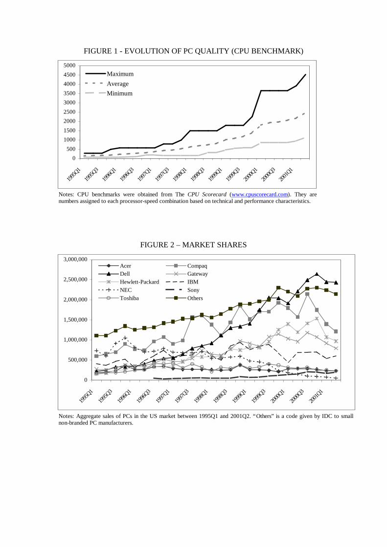
FIGURE 1 - EVOLUTION OF PC QUALITY (CPU BENCHMARK)

Notes: CPU benchmarks were obtained from The CPU Scorecard (www.cpuscorecard.com). They are numbers assigned to each processor-speed combination based on technical and performance characteristics.

FIGURE 2 – MARKET SHARES

Notes: Aggregate sales of PCs in the US market between 1995Q1 and 2001Q2. “Others” is a code given by IDC to small non-branded PC manufacturers.

0

500,000

1,000,000

1,500,000

2,000,000

2,500,000

3,000,000

1995Q

1

1995Q

3

1996Q

1

1996Q

3

1997Q

1

1997Q

3

1998Q

1

1998Q

3

1999Q

1

1999Q

3

2000Q

1

2000Q

3

2001Q

1

Acer CompaqDell GatewayHewlett-Packard IBMNEC SonyToshiba Others

0

500

1000

1500

2000

2500

3000

3500

4000

4500

5000

1995Q

1

1995Q

3

1996Q

1

1996Q

3

1997Q

1

1997Q

3

1998Q

1

1998Q

3

1999Q

1

1999Q

3

2000Q

1

2000Q

3

2001Q

1

MaximumAverageMinimum

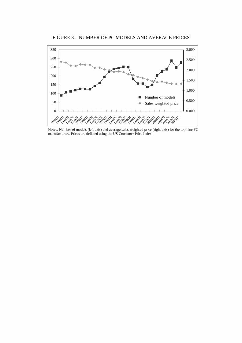
FIGURE 3 – NUMBER OF PC MODELS AND AVERAGE PRICES

Notes: Number of models (left axis) and average sales-weighted price (right axis) for the top nine PC manufacturers. Prices are deflated using the US Consumer Price Index.

0

50

100

150

200

250

300

350

1995Q

1

1995Q

2

1995Q

3

1995Q

4

1996Q

1

1996Q

2

1996Q

3

1996Q

4

1997Q

1

1997Q

2

1997Q

3

1997Q

4

1998Q

1

1998Q

2

1998Q

3

1998Q

4

1999Q

1

1999Q

2

1999Q

3

1999Q

4

2000Q

1

2000Q

2

2000Q

3

2000Q

4

2001Q

1

2001Q

2

0.000

0.500

1.000

1.500

2.000

2.500

3.000

Number of modelsSales weighted price

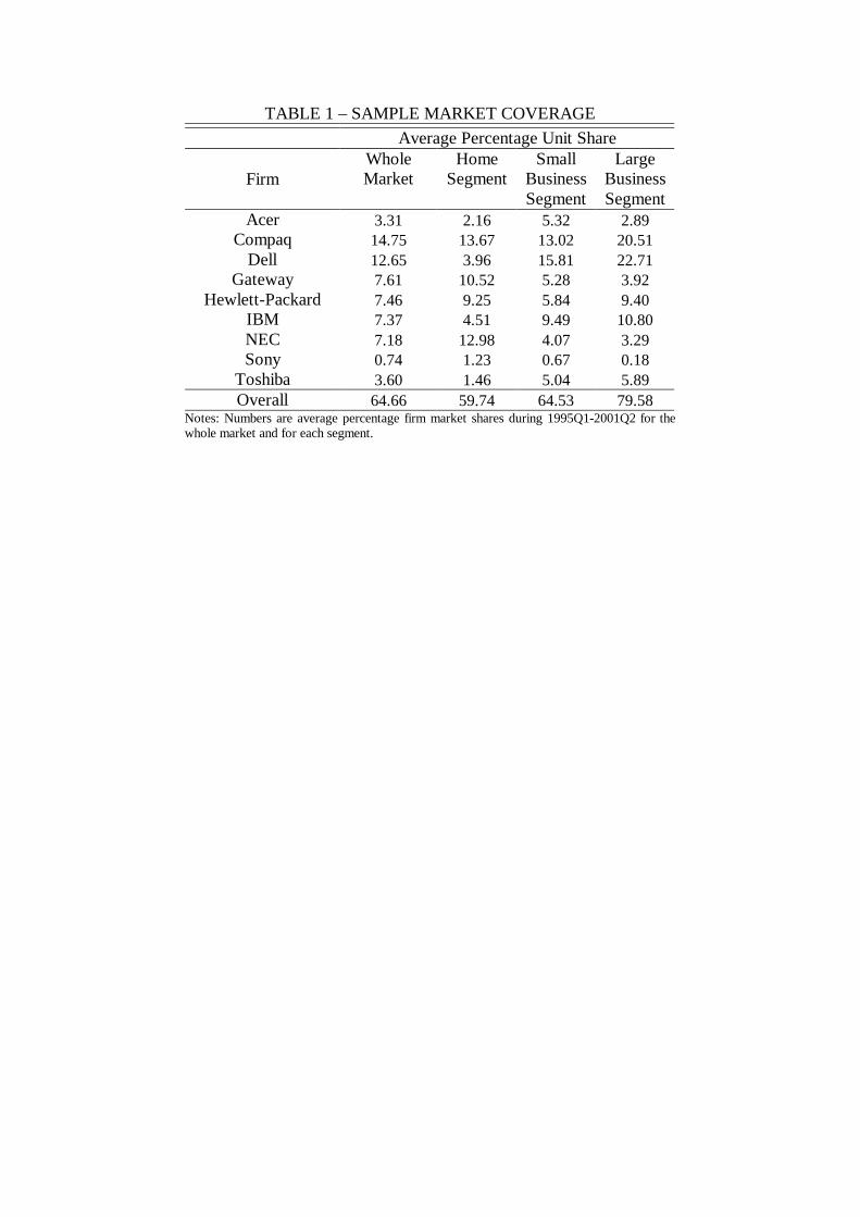
TABLE 1 – SAMPLE MARKET COVERAGE Average Percentage Unit Share

Firm Whole Market

Home Segment

Small Business Segment

Large Business Segment

Acer 3.31 2.16 5.32 2.89 Compaq 14.75 13.67 13.02 20.51

Dell 12.65 3.96 15.81 22.71 Gateway 7.61 10.52 5.28 3.92

Hewlett-Packard 7.46 9.25 5.84 9.40 IBM 7.37 4.51 9.49 10.80 NEC 7.18 12.98 4.07 3.29 Sony 0.74 1.23 0.67 0.18

Toshiba 3.60 1.46 5.04 5.89 Overall 64.66 59.74 64.53 79.58

Notes: Numbers are average percentage firm market shares during 1995Q1-2001Q2 for the whole market and for each segment.

TABLE 2 – DESCRIPTIVE STATISTICS FOR THE WHOLE MARKET

Period No. of models Quantity Price Benchmark RAM CD-ROM Internet Monitor

size Desktop

1995Q1 88 28.701 2.410 0.140 0.103 0.678 0.513 12.050 0.815 1995Q2 106 23.083 2.370 0.155 0.114 0.690 0.516 11.636 0.799 1995Q3 112 27.673 2.222 0.176 0.130 0.784 0.578 12.390 0.839 1995Q4 118 31.433 2.208 0.192 0.133 0.796 0.597 12.212 0.834 1996Q1 127 25.287 2.285 0.221 0.142 0.847 0.604 12.376 0.813 1996Q2 125 26.559 2.264 0.237 0.150 0.879 0.617 12.367 0.791 1996Q3 124 32.358 2.260 0.264 0.158 0.931 0.665 12.930 0.786 1996Q4 143 31.272 2.108 0.293 0.177 0.933 0.670 13.421 0.780 1997Q1 160 24.719 2.116 0.363 0.219 0.931 0.643 12.169 0.773 1997Q2 195 20.984 2.038 0.413 0.245 0.943 0.659 12.069 0.781 1997Q3 222 22.629 1.998 0.476 0.277 0.977 0.711 11.336 0.792 1997Q4 241 22.572 1.912 0.525 0.313 0.962 0.731 11.672 0.816 1998Q1 245 19.502 1.939 0.609 0.375 0.941 0.783 12.189 0.817 1998Q2 253 18.217 1.903 0.708 0.434 0.961 0.749 12.414 0.795 1998Q3 250 22.883 1.801 0.792 0.489 0.968 0.770 12.898 0.802 1998Q4 182 36.279 1.758 0.915 0.600 0.939 0.845 13.313 0.808 1999Q1 156 37.409 1.674 1.051 0.724 0.944 0.812 15.058 0.811 1999Q2 156 39.256 1.607 1.119 0.771 0.931 0.835 15.822 0.790 1999Q3 136 48.581 1.536 1.259 0.857 0.941 0.889 16.083 0.791 1999Q4 149 48.340 1.465 1.447 0.946 0.944 0.879 15.980 0.795 2000Q1 203 33.184 1.411 1.753 0.958 0.982 0.869 14.060 0.797 2000Q2 226 28.448 1.437 1.933 1.018 0.977 0.855 14.234 0.753 2000Q3 237 32.061 1.381 1.995 1.016 0.978 0.875 14.267 0.752 2000Q4 287 26.080 1.337 2.171 1.056 0.978 0.887 14.868 0.775 2000Q1 249 24.715 1.324 2.390 1.103 0.980 0.871 15.069 0.765 2000Q2 277 19.326 1.331 2.725 1.231 0.975 0.886 15.225 0.730

ALL 4767 27.804 1.752 1.114 0.624 0.934 0.777 13.706 0.789 Note: All entries in the last seven columns are sales weighted means.

TABLE 3 – DESCRIPTIVE STATISTICS FOR THE HOME SEGMENT

Period No. of models Quantity Price Benchmark RAM CD-ROM Modem Monitor

size Desktop

1995Q1 67 16.206 2.065 0.147 0.105 0.735 0.673 14.139 0.917 1995Q2 78 11.614 1.992 0.161 0.113 0.765 0.681 13.995 0.891 1995Q3 85 15.477 1.916 0.181 0.129 0.859 0.767 14.263 0.927 1995Q4 87 19.069 1.929 0.197 0.134 0.867 0.787 14.196 0.926 1996Q1 76 16.962 2.032 0.223 0.147 0.928 0.842 14.689 0.946 1996Q2 82 12.720 1.996 0.231 0.148 0.929 0.808 14.545 0.920 1996Q3 83 18.474 2.036 0.264 0.160 0.974 0.856 14.635 0.924 1996Q4 92 19.611 1.729 0.291 0.174 0.988 0.892 15.040 0.955 1997Q1 101 15.157 1.747 0.364 0.228 0.986 0.875 12.607 0.956 1997Q2 125 10.517 1.641 0.393 0.238 0.991 0.900 13.265 0.944 1997Q3 141 12.655 1.665 0.460 0.263 0.998 0.919 11.561 0.950 1997Q4 153 13.882 1.663 0.521 0.306 0.997 0.908 12.971 0.967 1998Q1 150 11.551 1.730 0.620 0.366 0.999 0.901 13.852 0.965 1998Q2 163 8.674 1.702 0.731 0.443 0.999 0.867 13.703 0.961 1998Q3 167 11.356 1.660 0.824 0.514 0.999 0.873 13.423 0.955 1998Q4 134 18.841 1.575 0.933 0.623 0.998 0.849 13.132 0.930 1999Q1 117 19.906 1.485 1.030 0.798 0.983 0.888 15.059 0.922 1999Q2 119 17.462 1.395 1.125 0.886 0.941 0.914 15.538 0.887 1999Q3 107 23.779 1.325 1.243 0.940 0.924 0.949 16.041 0.904 1999Q4 114 29.071 1.278 1.425 0.978 0.923 0.914 16.231 0.902 2000Q1 167 19.321 1.229 1.755 0.876 0.988 0.874 14.147 0.900 2000Q2 169 14.631 1.226 1.891 0.938 0.981 0.860 14.674 0.857 2000Q3 179 17.442 1.151 1.906 0.904 0.976 0.878 14.701 0.863 2000Q4 199 16.198 1.112 2.112 0.988 0.973 0.861 15.688 0.886 2000Q1 167 13.873 1.097 2.361 1.059 0.971 0.806 16.739 0.874 2000Q2 195 9.285 1.122 2.727 1.221 0.959 0.798 16.799 0.828

ALL 3317 15.494 1.504 1.118 0.627 0.957 0.863 14.602 0.913 Note: All entries in the last seven columns are sales weighted means.

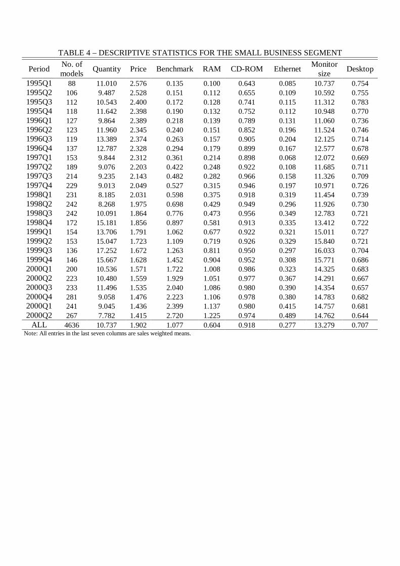
TABLE 4 – DESCRIPTIVE STATISTICS FOR THE SMALL BUSINESS SEGMENT

Period No. of models Quantity Price Benchmark RAM CD-ROM Ethernet Monitor

size Desktop

1995Q1 88 11.010 2.576 0.135 0.100 0.643 0.085 10.737 0.754 1995Q2 106 9.487 2.528 0.151 0.112 0.655 0.109 10.592 0.755 1995Q3 112 10.543 2.400 0.172 0.128 0.741 0.115 11.312 0.783 1995Q4 118 11.642 2.398 0.190 0.132 0.752 0.112 10.948 0.770 1996Q1 127 9.864 2.389 0.218 0.139 0.789 0.131 11.060 0.736 1996Q2 123 11.960 2.345 0.240 0.151 0.852 0.196 11.524 0.746 1996Q3 119 13.389 2.374 0.263 0.157 0.905 0.204 12.125 0.714 1996Q4 137 12.787 2.328 0.294 0.179 0.899 0.167 12.577 0.678 1997Q1 153 9.844 2.312 0.361 0.214 0.898 0.068 12.072 0.669 1997Q2 189 9.076 2.203 0.422 0.248 0.922 0.108 11.685 0.711 1997Q3 214 9.235 2.143 0.482 0.282 0.966 0.158 11.326 0.709 1997Q4 229 9.013 2.049 0.527 0.315 0.946 0.197 10.971 0.726 1998Q1 231 8.185 2.031 0.598 0.375 0.918 0.319 11.454 0.739 1998Q2 242 8.268 1.975 0.698 0.429 0.949 0.296 11.926 0.730 1998Q3 242 10.091 1.864 0.776 0.473 0.956 0.349 12.783 0.721 1998Q4 172 15.181 1.856 0.897 0.581 0.913 0.335 13.412 0.722 1999Q1 154 13.706 1.791 1.062 0.677 0.922 0.321 15.011 0.727 1999Q2 153 15.047 1.723 1.109 0.719 0.926 0.329 15.840 0.721 1999Q3 136 17.252 1.672 1.263 0.811 0.950 0.297 16.033 0.704 1999Q4 146 15.667 1.628 1.452 0.904 0.952 0.308 15.771 0.686 2000Q1 200 10.536 1.571 1.722 1.008 0.986 0.323 14.325 0.683 2000Q2 223 10.480 1.559 1.929 1.051 0.977 0.367 14.291 0.667 2000Q3 233 11.496 1.535 2.040 1.086 0.980 0.390 14.354 0.657 2000Q4 281 9.058 1.476 2.223 1.106 0.978 0.380 14.783 0.682 2000Q1 241 9.045 1.436 2.399 1.137 0.980 0.415 14.757 0.681 2000Q2 267 7.782 1.415 2.720 1.225 0.974 0.489 14.762 0.644

ALL 4636 10.737 1.902 1.077 0.604 0.918 0.277 13.279 0.707 Note: All entries in the last seven columns are sales weighted means.

TABLE 5 – DESCRIPTIVE STATISTICS FOR THE LARGE BUSINESS SEGMENT

Period No. of models Quantity Price Benchmark RAM CD-ROM Ethernet Monitor

size Desktop

1995Q1 74 6.365 2.839 0.133 0.105 0.616 0.127 9.936 0.708 1995Q2 88 6.083 2.697 0.152 0.117 0.626 0.150 9.605 0.726 1995Q3 93 6.484 2.541 0.172 0.133 0.705 0.155 10.416 0.757 1995Q4 98 6.901 2.510 0.187 0.132 0.712 0.154 9.915 0.735 1996Q1 104 6.439 2.550 0.221 0.138 0.799 0.187 10.388 0.703 1996Q2 103 7.823 2.437 0.240 0.151 0.863 0.254 11.089 0.706 1996Q3 99 8.946 2.441 0.266 0.157 0.905 0.279 11.426 0.674 1996Q4 114 8.034 2.437 0.294 0.178 0.889 0.236 11.845 0.628 1997Q1 129 7.116 2.409 0.363 0.213 0.896 0.091 11.596 0.637 1997Q2 156 6.807 2.255 0.424 0.248 0.919 0.127 11.209 0.692 1997Q3 181 6.979 2.210 0.489 0.287 0.963 0.177 11.035 0.698 1997Q4 193 6.486 2.123 0.531 0.321 0.931 0.217 10.626 0.709 1998Q1 204 5.660 2.101 0.609 0.388 0.892 0.378 10.898 0.723 1998Q2 219 5.453 2.019 0.695 0.430 0.936 0.335 11.705 0.708 1998Q3 215 6.428 1.885 0.775 0.483 0.947 0.417 12.382 0.734 1998Q4 143 10.259 1.896 0.914 0.595 0.884 0.453 13.447 0.749 1999Q1 131 10.657 1.810 1.069 0.670 0.914 0.436 15.128 0.755 1999Q2 124 14.063 1.705 1.124 0.701 0.926 0.454 16.137 0.763 1999Q3 113 15.190 1.663 1.279 0.796 0.955 0.446 16.213 0.741 1999Q4 122 13.124 1.619 1.487 0.938 0.973 0.401 15.757 0.727 2000Q1 152 9.228 1.592 1.792 1.073 0.963 0.384 13.461 0.731 2000Q2 179 9.047 1.585 2.001 1.091 0.972 0.418 13.481 0.719 2000Q3 194 9.266 1.554 2.085 1.109 0.977 0.440 13.385 0.703 2000Q4 233 7.366 1.555 2.206 1.110 0.986 0.513 13.453 0.707 2000Q1 197 8.413 1.493 2.417 1.120 0.993 0.517 13.143 0.721 2000Q2 222 6.598 1.472 2.730 1.252 0.995 0.623 13.936 0.732

ALL 3880 8.085 1.919 1.165 0.651 0.920 0.363 12.917 0.718 Note: All entries in the last seven columns are sales weighted means.

TABLE 6 – RESULTS FROM LOGIT DEMAND FOR THE WHOLE MARKET OLS IV Variables (1) (2) (3) (4) (5) (6) (7)

Price -0.33** (0.030)

-0.47** (0.031)

-0.69** (0.048)

-0.68** (0.049)

-0.70** (0.048)

-0.78** (0.267)

-2.74** (0.505)

Constant -9.22** (0.177)

-9.49** (0.187)

-8.89** (0.220)

-8.91** (0.233)

-8.87** (0.221)

-8.64** (0.772)

-3.08** (1.456)

Benchmark 0.32** (0.088)

0.32** (0.084)

0.44** (0.086)

0.44** (0.082)

0.45** (0.086)

0.49** (0.176)

1.61** (0.308)

RAM -0.35** (0.090)

-0.31** (0.089)

-0.16* (0.095)

-0.16* (0.096)

-0.15* (0.095)

-0.09 (0.207)

1.28** (0.377)

CD-ROM 0.09** (0.076)

0.13** (0.077)

0.15* (0.079)

0.15* (0.081)

0.15* (0.079)

0.16* (0.082)

0.29** (0.120)

Internet 0.22* (0.058)

0.34* (0.055)

0.32** (0.055)

0.32** (0.055)

0.32** (0.055)

0.31** (0.060)

0.16* (0.088)

Monitor Size -0.02** (0.005)

-0.02** (0.005)

-0.02** (0.005)

-0.02** (0.005)

-0.02** (0.005)

-0.02** (0.006)

-0.05** (0.010)

Desktop 0.62** (0.057)

0.57** (0.056)

0.41** (0.062)

0.41** (0.063)

0.40** (0.062)

0.34* (0.203)

-1.12** (0.384)

5th Generation 0.36** (0.111)

0.33** (0.117)

0.38** (0.122)

0.38** (0.131)

0.38** (0.122)

0.40** (0.139)

0.89** (0.222)

6th Generation 0.26* (0.149)

0.27* (0.150)

0.47** (0.156)

0.46** (0.161)

0.48** (0.156)

0.55* (0.285)

2.35** (0.512)

7th Generation 1.00** (0.263)

0.97** (0.262)

1.05** (0.262)

1.05** (0.286)

1.05** (0.262)

1.08** (0.274)

1.79** (0.442)

Firm Dummies no yes yes yes yes yes yes

Fit/Test of Over Identification

0.130

0.229

- -

31.39 (16.81)

63.61 (20.09)

31.24 (15.08)

18.064 (18.47)

1st Stage R2 0.461 0.4628 0.464 0.0166 0.0084 1st Stage F-test 4043.8 777.2 452.68 210.2 5.02 Instruments Canada prices X X X BLP IV X X “Modified” IV X X Own price elasticity Mean -0.68 -0.99 -1.43 -1.42 -1.45 -1.61 -5.69 Standard 0.29 0.42 0.61 0.60 0.62 0.69 2.42 Median -0.64 -0.92 -1.33 -1.32 -1.35 -1.51 -5.32 % of inelastic demands 88.44 58.38 23.79 24.29 22.74 16.45 0

Notes: The dependent variable is ln(Sjt)-ln(S0t). Based on 4,767 observations for the whole market. All regressions include time dummy variables. Asymptotically robust standard errors are reported in parentheses. * Z-statistic>1. ** Z-statistic>2. Adjusted R2 for the OLS regressions and the Hansen-Sargan test of overidentification for the IV regressions with the 1% critical values in parentheses. Canada prices are the prices of the same PC models in Canada; BLP IV are the sum of the values of the same characteristics of other products offered by the same firm, the sum of values of the same characteristics of all products offered by rival firms, the number of own-firm products and the number of rival firm products; “Modified” IV are the same as BLP IV, except that I condition on the form factor (see text for details).

TABLE 7 – RESULTS FROM THE RANDOM COEFFICIENTS MODEL FOR THE WHOLE MARKET

IV Random coefficients

Variables (1) (2) Means

Price -2.74** (0.505)

-5.94** (1.386)

Constant -3.08** (1.456)

-1.24 (4.190)

Benchmark 1.61** (0.308)

2.59** (0.967)

RAM 1.28** (0.377)

1.71** (0.732)

CD-ROM 0.29** (0.120)

0.32** (0.156)

Internet 0.16* (0.088)

0.11* (0.112)

Monitor Size -0.05** (0.010)

-0.06** (0.023)

Desktop -1.12** (0.384)

-5.14* (3.990)

5th Generation 0.89** (0.222)

1.35** (0.339)

6th Generation 2.35** (0.512)

3.84** (0.907)

7th Generation 1.79** (0.442)

2.25** (0.735)

Standard Deviations

Price 1.26**

(0.604)

Constant 2.50*

(2.143)

Benchmark 0.13

(3.122)

Desktop 3.88*

(2.954) GMM Objective (df) 3.52 (3)

Notes: Based on 4,767 observations for the whole market. All regressions include firm and time dummy variables. Asymptotically robust standard errors are reported in parentheses. * Z-statistic>1. ** Z-statistic>2. The first column is the same as column (7) in table 6. The second column presents parameters estimated via the two-step GMM algorithm described in the estimation subsection. The standard errors reported for the random coefficients take into account the variance introduced through the simulation by bootstrapping fifty times the relevant component of the variance in the moment conditions.

TABLE 8 – SAMPLE OF ESTIMATED SEMI-ELASTICITIES

Model Form Brand Price Benchmark Sales Markup Acer Desk AcerPower 2,476 97 28,783 246.900 Acer Desk AcerPower 3,382 272 7,196 323.280 Acer Desk AcerPower 2,775 142 23,986 270.600 Acer Desk Acros 2,506 97 25,154 249.180 Acer Desk Acros 2,785 217 4,791 271.180

-210.097 [-136.836]

0.449 [0.005]

1.519 [0.016]

1.543 [0.017]

0.303 [0.003]

1.794 [0.020]

-162.145 [-136.851]

1.895 [0.016]

1.609 [0.017]

0.380 [0.003]

1.822 [0.020]

0.568 [0.005]

-192.317 [-136.840]

1.612 [0.017]

0.338 [0.003]

1.765 [0.020]

0.460 [0.005]

1.538 [0.016]

-208.454 [-136.838]

0.307 [0.003]

1.824 [0.020]

0.571 [0.005]

1.695 [0.016]

1.615 [0.017]

-193.264 [-136.852]

Notes: The upper panel of the table gives the sample of Acer models in 1995Q1 for which the semi-elasticities are calculated in the lower panel. Cell entries in the lower panel are indexed i,j, where i indexes row and j column. Semi-elasticities are defined here as the percentage change in market share of i from a $500 change in the price of j. The first number in each cell provides the semi-elasticity calculated from the random coefficient model, whereas the second number is calculated from the IV logit model.

TABLE 9 – ESTIMATED MARKUPS AND MARGINS FOR THE WHOLE MARKET OLS Logit Instrumental Variable

Logit Random Coefficient

Logit Statistic (1) (2) (3) (4) (5) Median 2113.20 366.38 18.86% 250.38 13.39% Mean 2114.30 366.56 20.95% 269.59 14.11% 10% 2109.40 365.70 11.61% 201.91 10.36% 90% 2121.80 367.86 33.24% 355.46 18.75%

Standard Deviation 4.64 0.80 9.39% 85.80 3.89% Notes: Columns (1), (2) and (4) give statistics for the estimated distribution of markups over the whole period 1995Q1-2001Q2. Columns (3) and (5) provide statistics for the estimated distribution of margins. Margins are defined as markups divided by observed prices. All prices have been deflated using the US Consumer Price Index.

TABLE 10 – RESULTS OF THE DEMAND ESTIMATION FOR THE DIFFERENT SEGMENTS Home Segment Small Business Segment Large Business Segment OLS IV Random

Coefficients OLS IV Random

Coefficients OLS IV Random

Coefficients Variables (1) (2) (3) (4) (5) (6) (7) (8) (9)

Means

Price -0.76** (0.071)

-5.07** (0.534)

-6.410** (1.123)

-0.36** (0.033)

-3.09** (0.498)

-5.831** (2.002)

-0.30** (0.034)

-1.58** (0.313)

-5.771** (1.566)

Constant -10.64** (0.327)

1.28 (1.529)

1.284 (1.944)

-8.56** (0.199)

-0.71 (1.469)

1.138 (4.001)

-9.56** (0.202)

-5.83** (0.939)

-6.008 (6.654)

Benchmark 0.27** (0.130)

2.73** (0.346)

1.372 (1.523)

0.26** (0.095)

1.71** (0.294)

2.714** (0.781)

0.38** (0.097)

1.12** (0.213)

2.263** (0.799)

RAM -0.08 (0.156)

0.83** (0.255)

0.755** (0.270)

-0.34** (0.091)

1.47** (0.392)

2.083** (0.696)

-0.42** (0.093)

0.48* (0.254)

0.615* (0.387)

CD-ROM 0.04 (0.136)

0.46** (0.184)

0.377* (0.214)

0.27** (0.076)

0.28** (0.127)

0.234* (0.170)

0.28** (0.080)

0.35** (0.100)

0.340** (0.128)

Internet 1.20** (0.079)

0.83** (0.120)

0.761** (0.125)

0.14** (0.065)

0.96** (0.195)

1.314** (0.386)

0.08* (0.070)

0.32** (0.102)

0.365** (0.182)

Monitor Size -0.01* (0.008)

0.02* (0.013)

0.026** (0.013)

-0.03** (0.007)

-0.07** (0.012)

-0.085** (0.019)

-0.06** (0.007)

-0.08** (0.009)

-0.082** (0.018)

Desktop 1.30** (0.101)

-2.57** (0.493)

-7.115* (4.159)

0.24** (0.058)

-1.96** (0.407)

-8.568* (5.587)

0.40** (0.064)

-0.53** (0.233)

-2.597* (1.500)

5th Generation 0.34* (0.184)

1.66** (0.321)

1.808** (0.418)

0.37** (0.118)

1.05** (0.250)

1.510** (0.481)

0.29** (0.121)

0.63** (0.182)

1.207** (0.424)

6th Generation 0.76** (0.238)

4.69** (0.589)

5.101** (0.745)

0.30** (0.154)

2.81** (0.523)

4.433** (1.418)

0.04 (0.162)

1.22** (0.342)

2.673** (0.899)

7th Generation 1.79** (0.363)

3.53** (0.614)

3.609** (0.648)

0.58** (0.279)

1.90** (0.499)

2.511** (0.863)

0.02 (0.291)

0.58* (0.361)

1.025** (0.511)

Standard Deviations

Price 0.882** (0.444) 1.042*

(0.609) 1.792** (0.712)

Constant

0.759 (1.179) 2.377

(2.652) 4.399* (3.810)

Benchmark

1.377** (0.647) 0.051

(1.885) 0.102 (5.285)

Desktop

4.374* (2.327) 5.370*

(4.003) 2.555* (2.043)

Notes: All regressions include firm and time dummy variables. Asymptotically robust standard errors are reported in parentheses. * Z-statistic>1. ** Z-statistic>2. Parameters for the random coefficients model are estimated via the two-step GMM algorithm described in the estimation subsection. The standard errors reported take into account the variance introduced through the simulation by bootstrapping fifty times the relevant component of the variance in the moment conditions. The internet dummy equals one if the PC includes as standard a modem (for the home segment) or an ethernet card (for the small and large business segments).

TABLE 11 – ESTIMATED AGGREGATE ELASTICITIES

Whole Market

Home Segment

Small Business Segment

Large Business Segment

Mean (1) (2) (3) (4) IV Logit 4.95 7.94 5.93 3.17

Random Coefficients 3.94 4.70 4.17 2.62 Median IV Logit 5.10 8.26 5.97 3.18

Random Coefficients 3.94 4.84 4.20 2.49 Notes: Aggregate demand elasticity is calculated as the percentage change in total market share from a one percent increase in the price of all products in the market. Results for the overall market and each segment separately are based on the estimated coefficients in Tables 7 and 10.

TABLE 12 – ESTIMATED MARKUPS AND MARGINS FROM ALTERNATIVE SPECIFICATIONS Use Hard Disk instead

of RAM Specification similar to

Goeree’s random coefficients model

Include ln(number of products)

Statistic (1) (2) (3) (4) (5) (6) Median 233.73 12.37% 242.22 12.71% 293.71 16.28% Mean 244.77 13.05% 255.59 13.51% 356.56 17.28% 10% 194.33 9.23% 197.07 9.81% 207.11 12.68% 90% 304.79 17.78% 328.77 18.29% 541.89 22.28%

Standard Deviation 54.09 3.82% 64.18 3.85% 380.15 7.87% Number of significant random

coefficients variables 3 out of 4 1 out of 4 2 out of 4

Notes: Columns (1), (3) and (5) give statistics for the estimated distribution of markups from the various specifications. Columns (2), (4) and (6) present statistics for the estimated distribution of margins. A random coefficients variable is considered significant if either its mean or standard deviation of the taste distribution is significant (see text for details).

TABLE 13 – PREDICTED CHANGES DUE TO MERGERS IN PRICES, QUANTITIES AND MARGINAL COSTS 1995Q2 1998Q2 2001Q2 HP and

Compaq Dell and Compaq

HP and Compaq

Dell and Compaq

HP and Compaq

Dell and Compaq

%p %q %p %q %p %q %p %q %p %q %p %q Mean 0.58 -4.80 0.84 -6.72 1.00 -6.95 1.31 -8.67 1.11 -5.37 1.87 -9.00 Merging Median 0.48 -4.07 0.76 -5.54 1.06 -7.31 1.26 -8.66 0.60 -3.29 1.63 -7.59 Mean 0.02 0.73 0.03 1.26 0.02 1.31 0.03 0.93 0.01 0.73 0.04 0.63 Non-Merging Median 0.02 0.27 0.02 0.42 0.01 0.49 0.02 0.18 0.00 0.20 0.02 0.13

%mc %mc %mc %mc %mc %mc Mean 0.8 1.1 1.2 1.6 1.5 2.5

Median 0.7 1.1 1.2 1.4 0.8 1.9 Max 2.1 2.0 2.9 3.0 6.3 10.3

Merging

Min 0.2 0.4 0.3 0.9 0.4 0.6 Notes: The top panel of the table shows the mean and the median percentage changes in prices and quantities of the merging and non-merging firms due to mergers at various points in time. The bottom panel presents statistics on the marginal cost reduction required for the postmerger prices to remain unchanged.

TABLE 14 – PREDICTED CHANGES IN VARIABLE PROFITS AND CONSUMER SURPLUS DUE TO MERGERS (in million of dollars) 1995Q2 1998Q2 2001Q2

HP and Compaq

Dell and Compaq

HP and Compaq

Dell and Compaq

HP and Compaq

Dell and Compaq

Consumer Surplus -0.65 -1.14 -0.89 -1.79 -1.06 -2.01 Average consumer

surplus (in $) -0.0033 -0.0057 -0.0042 -0.0084 -0.0048 -0.0090

Profits Revenues Profits Revenues Profits Revenues Profits Revenues Profits Revenues Profits Revenues Industry Total 5.64 -53.77 7.79 -62.68 12.05 -102.65 18.55 -190.93 12.73 -56.58 21.56 -183.02

Acer 0.60 5.78 0.82 7.99 0.77 5.94 1.32 10.03 0.73 3.45 1.43 6.65 Compaq 0.87 -35.60 1.18 -48.20 1.35 -82.50 1.60 -145.80 0.92 -57.00 0.01 -131.77

Dell 0.72 6.53 -0.11 -67.24 3.65 23.70 1.76 -153.00 6.15 25.90 5.39 -126.60 Gateway 0.81 7.04 1.12 9.95 1.89 13.85 3.20 23.03 2.00 9.18 3.95 17.88

HP -0.15 -56.06 0.73 8.00 0.31 -93.13 3.65 25.20 0.94 -49.93 6.18 24.15 IBM 0.92 7.61 1.29 10.82 1.57 12.05 2.62 19.57 1.42 8.10 3.17 17.82 NEC 1.52 8.41 2.27 12.61 1.84 12.48 3.06 20.53 0.07 0.42 0.15 0.84 Sony 0.00 0.00 0.00 0.00 0.18 1.61 0.31 2.74 0.34 2.32 0.84 5.43

Toshiba 0.35 2.52 0.48 3.39 0.49 3.35 1.03 6.77 0.16 0.98 0.44 2.58

Total Welfare 4.99 6.65 11.16 16.76 11.67 19.55 Notes: Calculated changes in variable profits, revenues and consumer surplus as a result of the mergers. All numbers are in million of dollars, except for the average consumer surplus which is in dollars. Total welfare is calculated as consumer surplus plus profits.

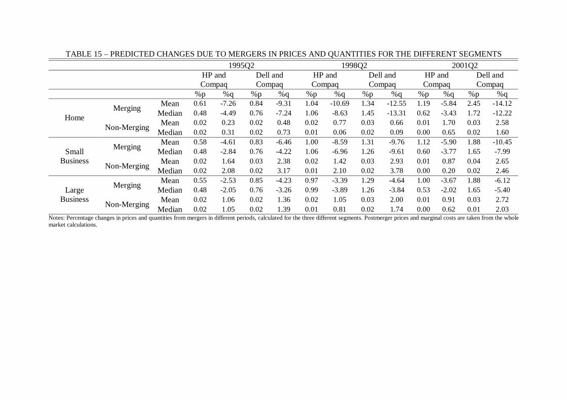
TABLE 15 – PREDICTED CHANGES DUE TO MERGERS IN PRICES AND QUANTITIES FOR THE DIFFERENT SEGMENTS 1995Q2 1998Q2 2001Q2

HP and Compaq

Dell and Compaq

HP and Compaq

Dell and Compaq

HP and Compaq

Dell and Compaq

%p %q %p %q %p %q %p %q %p %q %p %q Mean 0.61 -7.26 0.84 -9.31 1.04 -10.69 1.34 -12.55 1.19 -5.84 2.45 -14.12 Merging Median 0.48 -4.49 0.76 -7.24 1.06 -8.63 1.45 -13.31 0.62 -3.43 1.72 -12.22 Mean 0.02 0.23 0.02 0.48 0.02 0.77 0.03 0.66 0.01 1.70 0.03 2.58

Home Non-Merging Median 0.02 0.31 0.02 0.73 0.01 0.06 0.02 0.09 0.00 0.65 0.02 1.60

Mean 0.58 -4.61 0.83 -6.46 1.00 -8.59 1.31 -9.76 1.12 -5.90 1.88 -10.45 Merging Median 0.48 -2.84 0.76 -4.22 1.06 -6.96 1.26 -9.61 0.60 -3.77 1.65 -7.99 Mean 0.02 1.64 0.03 2.38 0.02 1.42 0.03 2.93 0.01 0.87 0.04 2.65

Small Business

Non-Merging Median 0.02 2.08 0.02 3.17 0.01 2.10 0.02 3.78 0.00 0.20 0.02 2.46 Mean 0.55 -2.53 0.85 -4.23 0.97 -3.39 1.29 -4.64 1.00 -3.67 1.88 -6.12 Merging Median 0.48 -2.05 0.76 -3.26 0.99 -3.89 1.26 -3.84 0.53 -2.02 1.65 -5.40 Mean 0.02 1.06 0.02 1.36 0.02 1.05 0.03 2.00 0.01 0.91 0.03 2.72

Large Business

Non-Merging Median 0.02 1.05 0.02 1.39 0.01 0.81 0.02 1.74 0.00 0.62 0.01 2.03 Notes: Percentage changes in prices and quantities from mergers in different periods, calculated for the three different segments. Postmerger prices and marginal costs are taken from the whole market calculations.

TABLE 16 – PREDICTED CHANGES IN VARIABLE PROFITS AND CONSUMER SURPLUS DUE TO MERGERS (in million of dollars) FOR THE HOME SEGMENT

1995Q2 1998Q2 2001Q2

HP and Compaq

Dell and Compaq

HP and Compaq

Dell and Compaq

HP and Compaq

Dell and Compaq

Consumer Surplus -0.17 -0.28 -0.36 -0.60 -0.71 -0.67 Average consumer

surplus (in $) -0.0017 -0.0028 -0.0035 -0.0058 -0.0067 -0.0063

Profits Revenues Profits Revenues Profits Revenues Profits Revenues Profits Revenues Profits Revenues Industry Total 2.34 7.98 2.66 3.22 1.69 -45.03 0.89 -56.85 4.82 -29.59 5.44 -58.78

Acer 0.07 0.54 0.12 1.06 0.12 0.90 0.12 0.86 0.12 0.50 0.13 0.54 Compaq -0.22 -8.02 -0.33 -11.87 -0.65 -30.76 -1.99 -57.15 -0.24 -26.46 -2.40 -60.89

Dell 0.03 0.18 -0.27 -8.38 0.36 2.33 -0.86 -23.74 2.40 11.29 -0.31 -33.45 Gateway 0.16 1.05 0.27 2.14 0.87 6.39 0.88 5.79 2.29 10.87 3.58 16.61

HP -0.12 -3.90 0.02 0.17 -0.93 -37.85 0.76 4.33 -0.26 -29.02 3.54 12.87 IBM 2.03 17.44 2.13 18.19 0.42 3.30 0.43 3.17 0.09 0.49 0.16 0.84 NEC 0.48 1.48 0.80 2.78 1.33 9.06 1.35 8.23 0.01 0.03 0.01 0.05 Sony 0.00 0.00 0.00 0.00 0.18 1.60 0.19 1.66 0.39 2.54 0.67 4.29

Toshiba -0.08 -0.79 -0.08 -0.87 0.00 0.00 0.00 -0.01 0.03 0.17 0.06 0.37

Total Welfare 2.17 2.38 1.33 0.29 4.11 4.77 Notes: Calculated changes in variable profits, revenues and consumer surplus as a result of the mergers. All numbers are in million of dollars, except for the average consumer surplus which is in dollars. Total welfare is calculated as consumer surplus plus profits.

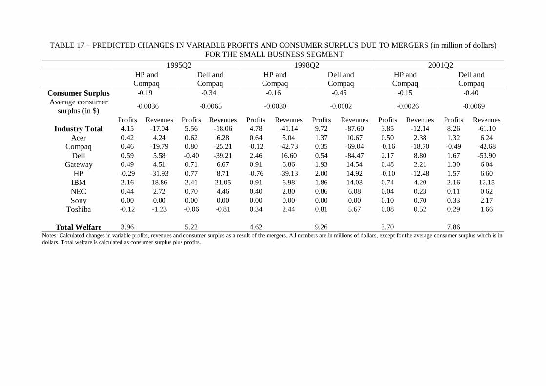
TABLE 17 – PREDICTED CHANGES IN VARIABLE PROFITS AND CONSUMER SURPLUS DUE TO MERGERS (in million of dollars) FOR THE SMALL BUSINESS SEGMENT

1995Q2 1998Q2 2001Q2

HP and Compaq

Dell and Compaq

HP and Compaq

Dell and Compaq

HP and Compaq

Dell and Compaq

Consumer Surplus -0.19 -0.34 -0.16 -0.45 -0.15 -0.40 Average consumer

surplus (in $) -0.0036 -0.0065 -0.0030 -0.0082 -0.0026 -0.0069

Profits Revenues Profits Revenues Profits Revenues Profits Revenues Profits Revenues Profits Revenues Industry Total 4.15 -17.04 5.56 -18.06 4.78 -41.14 9.72 -87.60 3.85 -12.14 8.26 -61.10

Acer 0.42 4.24 0.62 6.28 0.64 5.04 1.37 10.67 0.50 2.38 1.32 6.24 Compaq 0.46 -19.79 0.80 -25.21 -0.12 -42.73 0.35 -69.04 -0.16 -18.70 -0.49 -42.68

Dell 0.59 5.58 -0.40 -39.21 2.46 16.60 0.54 -84.47 2.17 8.80 1.67 -53.90 Gateway 0.49 4.51 0.71 6.67 0.91 6.86 1.93 14.54 0.48 2.21 1.30 6.04

HP -0.29 -31.93 0.77 8.71 -0.76 -39.13 2.00 14.92 -0.10 -12.48 1.57 6.60 IBM 2.16 18.86 2.41 21.05 0.91 6.98 1.86 14.03 0.74 4.20 2.16 12.15 NEC 0.44 2.72 0.70 4.46 0.40 2.80 0.86 6.08 0.04 0.23 0.11 0.62 Sony 0.00 0.00 0.00 0.00 0.00 0.00 0.00 0.00 0.10 0.70 0.33 2.17

Toshiba -0.12 -1.23 -0.06 -0.81 0.34 2.44 0.81 5.67 0.08 0.52 0.29 1.66

Total Welfare 3.96 5.22 4.62 9.26 3.70 7.86 Notes: Calculated changes in variable profits, revenues and consumer surplus as a result of the mergers. All numbers are in millions of dollars, except for the average consumer surplus which is in dollars. Total welfare is calculated as consumer surplus plus profits.

TABLE 18 – PREDICTED CHANGES IN VARIABLE PROFITS AND CONSUMER SURPLUS DUE TO MERGERS (in million of dollars) FOR THE LARGE BUSINESS SEGMENT

1995Q2 1998Q2 2001Q2

HP and Compaq

Dell and Compaq

HP and Compaq

Dell and Compaq

HP and Compaq

Dell and Compaq

Consumer Surplus -0.21 -0.38 -0.38 -0.65 -0.36 -0.91 Average consumer

surplus (in $) -0.0044 -0.0079 -0.0071 -0.0122 -0.0061 -0.0154

Profits Revenues Profits Revenues Profits Revenues Profits Revenues Profits Revenues Profits Revenues Industry Total 3.62 -3.03 4.18 -4.47 5.88 -13.77 10.19 -30.96 5.02 -8.05 13.65 -29.47

Acer 0.06 0.54 0.09 0.88 0.16 1.23 0.31 2.33 0.12 0.59 0.33 1.56 Compaq 0.54 -8.04 0.78 -9.89 1.64 -12.80 2.82 -23.12 1.02 -12.94 2.58 -27.99

Dell 0.15 1.25 0.96 -15.83 1.34 8.48 3.97 -31.61 2.33 9.70 6.89 -23.50 Gateway 0.07 0.53 0.10 0.83 0.27 2.00 0.52 3.84 0.12 0.56 0.33 1.58

HP 1.11 -11.38 0.38 4.27 1.81 -17.10 1.17 7.92 0.78 -9.65 1.59 8.00 IBM 1.85 16.11 1.92 16.69 0.35 2.37 0.72 5.08 0.54 3.07 1.60 8.89 NEC 0.06 0.15 0.12 0.54 0.12 0.87 0.25 1.80 0.03 0.16 0.08 0.45 Sony 0.00 0.00 0.00 0.00 0.00 0.00 0.00 0.00 0.02 0.12 0.06 0.44

Toshiba -0.22 -2.19 -0.18 -1.96 0.18 1.19 0.43 2.80 0.05 0.33 0.18 1.10

Total Welfare 3.41 3.80 5.50 9.54 4.66 12.74 Notes: Calculated changes in variable profits, revenues and consumer surplus as a result of the mergers. All numbers are in millions of dollars, except for the average consumer surplus which is in dollars. Total welfare is calculated as consumer surplus plus profits.