Differential geometry Lecture 14 ... - math.uni-hamburg.de
21
Differential geometry Lecture 14: Local frames and Killing vector fields David Lindemann University of Hamburg Department of Mathematics Analysis and Differential Geometry & RTG 1670 12. June 2020 David Lindemann DG lecture 14 12. June 2020 1 / 21
Transcript of Differential geometry Lecture 14 ... - math.uni-hamburg.de
Differential geometryLecture 14: Local frames and Killing vector fields
David Lindemann
University of HamburgDepartment of Mathematics
Analysis and Differential Geometry & RTG 1670
12. June 2020
David Lindemann DG lecture 14 12. June 2020 1 / 21

1 Local frames of vector bundles
2 Examples of subbundles
3 Killing vector fields
David Lindemann DG lecture 14 12. June 2020 2 / 21

Recap of lecture 13:
defined trace and induced scalar product in tensorbundles
explained how to raise and lower indices of tensor fields
defined vector bundles along submanifolds, in particulartangent and orthogonal bundle for pseudo-Riemanniansubmanifolds
erratum: called the position vector field “tangent” toHnν ⊂ Rn+1, correct would have been “orthogonal”
David Lindemann DG lecture 14 12. June 2020 3 / 21

Local frames of vector bundles
We know what a basis of a vector space is, and in the exampleof the tensor bundles of a smooth manifold T r,sM → M howto fibrewise obtain a basis of T r,s
p M via a choice of localcoordinates near p ∈ M.
Question: What is the correct local (not just fibrewise)setting for choosing bases of fibres over an open subset of thebase space of vector bundles, and how does it fit in with whatwe already learned?Answer: Define, locally, for each fibre a basis that variessmoothly.
Definition
Let E → M be a vector bundle of rank k. A (local) frame ofE over U ⊂ M, U open, is a set of k (local) sections
si ∈ Γ(E |U), 1 ≤ i ≤ k,
such that for all p ∈ U fixed, the vectors si (p) ∈ Ep, 1 ≤ i ≤ k,are linearly independent. Equivalently,
spanRsi (p) ∈ Ep | 1 ≤ i ≤ k = Ep ∀p ∈ U.
David Lindemann DG lecture 14 12. June 2020 4 / 21

Local frames of vector bundles
Examples
A local frame in TM → M over U ⊂ M is a set ofn = dim(M) local vector fields X1, . . . ,Xn ∈ X(U)such that, pointwise, X1p, . . . ,Xnp ∈ TpM are linearlyindependent.
Local coordinates (x1, . . . , xn) on U ⊂ M induce the localframe ∂
∂x1 , . . . ,∂∂xn of local coordinate vector fields in
TM → M over U.
Similarly, the local coordinate 1-forms dx1, . . . , dxnare a frame of T ∗M → M over U.
Local trivializations can be constructed from local frames:
Exercise
Suppose that you are given a local frame of E → M overU ⊂ M. Construct a local trivialization of E → M using thisdata.
David Lindemann DG lecture 14 12. June 2020 5 / 21
Local frames of vector bundles
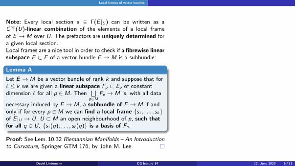
Note: Every local section s ∈ Γ(E |U) can be written as aC∞(U)-linear combination of the elements of a local frameof E → M over U. The prefactors are uniquely determined fora given local section.Local frames are a nice tool in order to check if a fibrewise linearsubspace F ⊂ E of a vector bundle E → M is a subbundle:
Lemma A
Let E → M be a vector bundle of rank k and suppose that for` ≤ k we are given a linear subspace Fp ⊂ Ep of constantdimension ` for all p ∈ M. Then
⊔p∈M
Fp → M is, with all data
necessary induced by E → M, a subbundle of E → M if andonly if for every p ∈ M we can find a local frame s1, . . . , skof E |U → U, U ⊂ M an open neighbourhood of p, such thatfor all q ∈ U, s1(q), . . . , s`(q) is a basis of Fq.
Proof: See Lem. 10.32 Riemannian Manifolds – An Introductionto Curvature, Springer GTM 176, by John M. Lee.
David Lindemann DG lecture 14 12. June 2020 6 / 21

Local frames of vector bundles
Lemma A implies the following for the local form of subbundles:
Corollary
Let F → M be a subbundle of rank ` of a vector bundleE → M of rank k > `. For any p ∈ M we can find an openneighbourhood U ⊂ M of p and a local trivialization ofE → M over U, φ : E |U → U × Rk , such that
φ(ι(F |U)) =
U × (v 1, . . . , v `, 0, . . . , 0) | (v 1, . . . , v `) ∈ R` ⊂ U × Rk ,
where ι denotes the inclusion.
David Lindemann DG lecture 14 12. June 2020 7 / 21

Examples of subbundles
Using the local frames, we will next describe two prominentsubbundles of the (0, 2)-tensor bundle of a smooth manifold.First, recall the following construction from linear algebra:
Lemma
Let V be a finite-dimensional real vector space with basisv1, . . . , vn. Then
V ⊗ V ∼= Sym2(V )⊕ Λ2V ,
where Sym2(V ) := spanRvi ⊗ vj + vj ⊗ vi , 1 ≤ i , j ≤ n andΛ2V := spanRvi ⊗ vj − vj ⊗ vi , 1 ≤ i , j ≤ n.
Notation: vivj := 12(vi⊗vj +vj⊗vi ), vi ∧vj := vi⊗vj−vj⊗vi ,
so that vi ⊗ vj = vivj + 12vi ∧ vj and vi ⊗ vi = vivi for all i , j
Question: How do we formulate a similar statement forT 0,2M → M?Answer: Fibrewise using local frames! (next page)
David Lindemann DG lecture 14 12. June 2020 8 / 21

Examples of subbundles
Definition
Let M be a smooth manifold and (x1, . . . , xn) be localcoordinates on U ⊂ M. The bundle of symmetric(0, 2)-tensors on M is the subbundle
Sym2(T ∗M) ⊂ T 0,2M
with local frame over U given bydx idx j = 1
2(dx i ⊗ dx j + dx j ⊗ dx i ), 1 ≤ i , j ≤ n
. Sections
of Sym2(T ∗M) are precisely symmetric (0, 2)-tensor fields,which in particular include all possible pseudo-Riemannianmetrics on M. On the other hand we have the anti-symmetric(0, 2)-tensors on M,
Λ2T ∗M ⊂ T 0,2M,
with local frame over U given bydx i ∧ dx j = dx i ⊗ dx j − dx j ⊗ dx i , 1 ≤ i , j ≤ n
. Sections in
Λ2T ∗M → M are called 2-forms and are denoted by Ω2(M).Local sections in Λ2T ∗M → M over U ⊂ M, U open, aredenoted by Ω2(U).
David Lindemann DG lecture 14 12. June 2020 9 / 21

Examples of subbundles
Remark
Any pseudo-Riemannian metric g on M can be written locallyas
g =∑i,j
gijdxi ⊗ dx j =
∑i,j
gijdxidx j .
Warning: The above notation is standard, but has a certain errorpotential. Make absolutely sure to e.g. understand the equality
dx dy “ = ”
(0 1
212
0
),
where in the above equation dx dy is written on the right handside in (in actual calculations commonly used) matrix nota-tion.
David Lindemann DG lecture 14 12. June 2020 10 / 21
Examples of subbundles
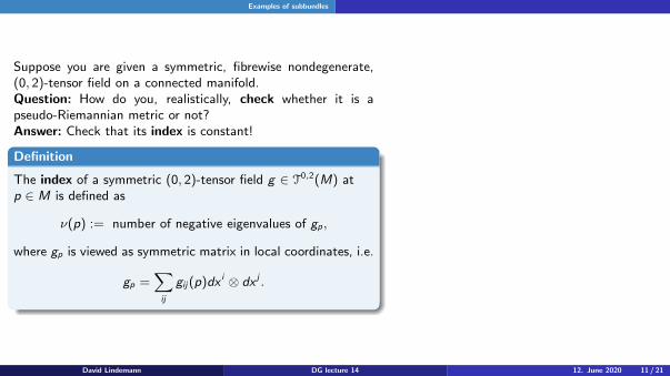
Suppose you are given a symmetric, fibrewise nondegenerate,(0, 2)-tensor field on a connected manifold.Question: How do you, realistically, check whether it is apseudo-Riemannian metric or not?Answer: Check that its index is constant!
Definition
The index of a symmetric (0, 2)-tensor field g ∈ T0,2(M) atp ∈ M is defined as
ν(p) := number of negative eigenvalues of gp,
where gp is viewed as symmetric matrix in local coordinates, i.e.
gp =∑ij
gij(p)dx i ⊗ dx j .
David Lindemann DG lecture 14 12. June 2020 11 / 21

Examples of subbundles
Proposition
Let M be a connected smooth manifold and g ∈ T0,2(M) asymmetric (0, 2)-tensor field that is nondegenerate in allfibres TpM, p ∈ M. Then g is a pseudo-Riemannian metric.
Proof:
suffices to show that the index of g , ν : M → N0, iscontinuous
for this it suffices to prove that the number of negativeeigenvalues of any smooth function with values in thesymmetric n × n-matrices,
A : I → Sym2((R∗)n), t 7→ A(t) ∈ Sym2((R∗)n),
such that A(t) is nondegenerate for all t ∈ I , is locallyconstant
this follows from the continuity of the eigenvalues ofA(t) viewed each as functions of t
(continued on next page)David Lindemann DG lecture 14 12. June 2020 12 / 21

Examples of subbundles
(continuation of proof)
[more precisely: There exists a choice of n nowherevanishing continuous functions λn : I → R \ 0, such thatfor all t ∈ I , the set (1, λ1(t)), . . . , (n, λn(t)) is preciselythe set of (indexed) eigenvalues of A(t)]
consider the characteristic polynomial of A(t) independence of t ∈ I ,
Pt(λ) := det(A(t)− λ1)
Pt(λ) is of the form
Pt(λ) =n∑
i=0
ai (t)λi ,
where ai : I → R is smooth for all 0 ≤ i ≤ n andan(t) ≡ (−1)n
(continued on next page)
David Lindemann DG lecture 14 12. June 2020 13 / 21

Examples of subbundles
(continuation of proof)
hence: suffices to prove continuous dependence of rootsof a polynomial of fixed degree with smoothly varyingprefactors and fixed highest order monomial
we know that the eigenvalues must be real by thesymmetry condition of A(t) and can use the main resultin Continuity and Location of Zeroes of LinearCombinations of Polynomials (M. Zedek), Proc. Amer.Math. Soc. 16 (1965)
David Lindemann DG lecture 14 12. June 2020 14 / 21

Killing vector fields
Recall the definition of isometries of pseudo-Riemannian mani-folds and note that the identity map is an isometry in any case.Question: How can we describe isometries infinitesimally, as ininfinitesimal perturbations of the identity?Answer: Use local flows and the Lie derivative of tensor fields!
Proposition
Let (M, g) be a pseudo-Riemannian manifold and letX ∈ X(M). Suppose that for every local flow ϕ : I × U → Mof X , ϕt : U → M is an isometry for all t ∈ I . Then LXg = 0.The converse statement also holds true.
Proof:
“⇒”: a local flow ϕ : I × U → M of X is an isometry of(M, g) for all t ∈ I if and only if
gp(v ,w) = gϕt (p)(dϕt(v), dϕt(w))
for all t ∈ I , p ∈ M, v ,w ∈ TpM
(continued on next page)
David Lindemann DG lecture 14 12. June 2020 15 / 21
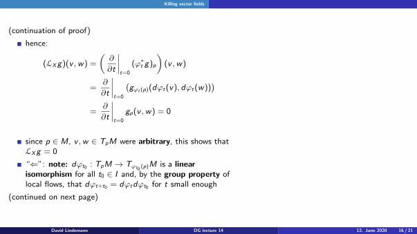
Killing vector fields
(continuation of proof)
hence:
(LXg)(v ,w) =
(∂
∂t
∣∣∣∣t=0
(ϕ∗t g)p
)(v ,w)
=∂
∂t
∣∣∣∣t=0
(gϕt (p)(dϕt(v), dϕt(w))
)=
∂
∂t
∣∣∣∣t=0
gp(v ,w) = 0
since p ∈ M, v ,w ∈ TpM were arbitrary, this shows thatLXg = 0
“⇐”: note: dϕt0 : TpM → Tϕt0(p)M is a linear
isomorphism for all t0 ∈ I and, by the group property oflocal flows, that dϕt+t0 = dϕtdϕt0 for t small enough
(continued on next page)
David Lindemann DG lecture 14 12. June 2020 16 / 21

Killing vector fields
(continuation of proof)
we obtain ∀t0 ∈ I , v ,w ∈ TpM
0 = (LXg)(dϕt0 (v), dϕt0 (w))
=∂
∂t
∣∣∣∣t=0
(gϕt (ϕt0
(p))(dϕtdϕt0 (v), dϕtdϕt0 (w)))
=∂
∂t
∣∣∣∣t=0
(gϕt+t0
(p)(dϕt+t0 (v), dϕt+t0 (w)))
=∂
∂s
∣∣∣∣s=t0
(gϕs (p)(dϕs(v), dϕs(w))
)this shows that the smooth function
I 3 s 7→ gϕs (p)(dϕs(v), dϕs(w)) ∈ R
is constant for all v ,w ∈ TpM and, hence, that the localflow of X consists of isometries for any fixed timeparameter
David Lindemann DG lecture 14 12. June 2020 17 / 21
Killing vector fields
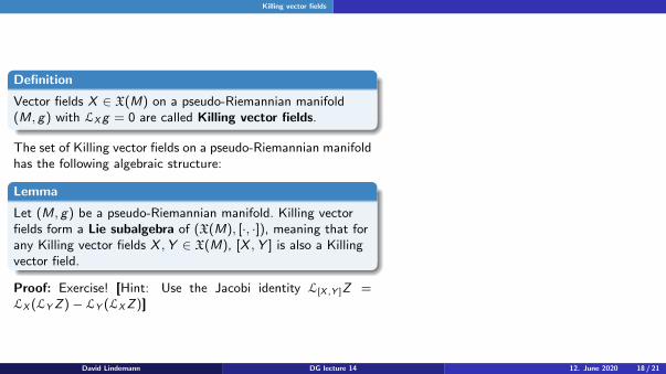
Definition
Vector fields X ∈ X(M) on a pseudo-Riemannian manifold(M, g) with LXg = 0 are called Killing vector fields.
The set of Killing vector fields on a pseudo-Riemannian manifoldhas the following algebraic structure:
Lemma
Let (M, g) be a pseudo-Riemannian manifold. Killing vectorfields form a Lie subalgebra of (X(M), [·, ·]), meaning that forany Killing vector fields X ,Y ∈ X(M), [X ,Y ] is also a Killingvector field.
Proof: Exercise! [Hint: Use the Jacobi identity L[X ,Y ]Z =LX (LYZ)− LY (LXZ)]
David Lindemann DG lecture 14 12. June 2020 18 / 21
Killing vector fields
One can prove the following theorem about a dimensional boundof the Lie algebra of Killing vector fields, but the proof goes farbeyond the scope of this course, cf. Thm 3.3 in Foundations ofDifferential Geometry Vol. I (S. Kobayashi, K. Nomizu), WileyClassics Library (1996)
Theorem
Let (M, g) be a connected Riemannian manifold ofdimension n. The the Lie algebra of Killing vector fields isfinite dimensional of dimension at most 1
2n(n + 1).
Next, let us look at some examples of Killing vector fields. (nextpage)
David Lindemann DG lecture 14 12. June 2020 19 / 21

Killing vector fields
Examples
Consider (M, g) = (Rn, 〈·, ·〉ν) for any 0 ≤ ν ≤ n. ThenX ∈ X(Rn), X =
∑i
c i ∂∂ui
, is a Killing vector field.
Let (M, g) and (N, h) be pseudo-Riemannian manifolds,X a Killing vector field on (M, g), and Y a Killing vectorfield on (N, h). Then X + Y is a Killing vector field on(M × N, g ⊕ h).
Question: How can we determine Killing vector fields if we arenot magically presented with them?Answer: In local coordinates, have the following result:
Lemma
X ∈ X(M) on a pseudo-Riemannian manifold (M, g) is aKilling vector field if and and only if it fulfils
n∑k=1
(X k ∂gij
∂xk+∂X k
∂x igjk +
∂X k
∂x jgik
)= 0 ∀1 ≤ i , j ≤ n
for all local coordinates (x1, . . . , xn) on M.
Proof: Exercise!David Lindemann DG lecture 14 12. June 2020 20 / 21

END OF LECTURE 14
Next lecture:
connections in vector bundles
David Lindemann DG lecture 14 12. June 2020 21 / 21