Differential Flatness of Quadrotor Dynamics Subject to Rotor Drag forAccurate Tracking of High-Speed Trajectories

Matthias Faessler1, Antonio Franchi2, and Davide Scaramuzza1

Abstract— In this paper, we prove that the dynamical modelof a quadrotor subject to linear rotor drag effects is differen-tially flat in its position and heading. We use this property tocompute feed-forward control terms directly from a referencetrajectory to be tracked. The obtained feed-forward terms arethen used in a cascaded, nonlinear feedback control law thatenables accurate agile flight with quadrotors. Compared tostate-of-the-art control methods, which treat the rotor dragas an unknown disturbance, our method reduces the trajectorytracking error significantly. Finally, we present a method basedon a gradient-free optimization to identify the rotor dragcoefficients, which are required to compute the feed-forwardcontrol terms. The new theoretical results are thoroughlyvalidated trough extensive comparative experiments.

SUPPLEMENTARY MATERIAL

Video: https://youtu.be/VIQILwcM5PACode: https://github.com/uzh-rpg/rpg quadrotor control

I. INTRODUCTION

A. Motivation

For several years, quadrotors have proven to be suitableaerial platforms for performing agile flight maneuvers. Nev-ertheless, quadrotors are typically controlled by neglectingaerodynamic effects, such as rotor drag, that only becomeimportant for non-hover conditions. These aerodynamic ef-fects are treated as unknown disturbances, which works wellwhen controlling the quadrotor close to hover conditions butreduces its trajectory tracking accuracy progressively withincreasing speed. For fast obstacle avoidance it is importantto perform accurate agile trajectory tracking. To achieve this,we require a method for accurate tracking of trajectories thatare unknown prior to flying.

The main aerodynamic effect causing trajectory trackingerrors during high-speed flight is rotor drag, which is alinear effect in the quadrotor’s velocity [1]. In this work,we aim at developing a control method that improves thetrajectory tracking performance of quadrotors by consideringthe rotor drag effect. To achieve this, we first prove thatthe dynamical model of a quadrotor subject to linear rotordrag effects is differentially flat with flat outputs chosento be its position and heading. We then use this property

This research was supported by the National Centre of Competence inResearch (NCCR) Robotics, the SNSF-ERC Starting Grant, the DARPAFLA program, and the European Union’s Horizon 2020 research andinnovation program under grant agreement No 644271 AEROARMS.

1The two authors are with the Robotics and Perception Group, Dep.of Informatics University of Zurich and Dep. of Neuroinformatics of theUniversity of Zurich and ETH Zurich, Switzerland—http://rpg.ifi.uzh.ch.

2Antonio Franchi is with LAAS-CNRS, Universite de Toulouse, CNRS,Toulouse, France.

Fig. 1: First-person-view racing inspired quadrotor platform usedfor the presented experiments.

to compute feed-forward control terms directly from thereference trajectory to be tracked. The obtained feed-forwardterms are then used in a cascaded, nonlinear feedback controllaw that enables accurate agile flight with quadrotors on apriori unknown trajectories. Finally, we present a methodbased on a gradient-free optimization to identify the rotordrag coefficients which are required to compute the feed-forward control terms. We validate our theoretical resultsthrough experiments with a quadrotor shown in Fig. 1.

B. Related Work

In [2], it was shown that the common model of a quadrotorwithout considering rotor drag effects is differentially flatwhen choosing its position and heading as flat outputs.Furthermore, this work presented a control algorithm thatcomputes the desired collective thrust and torque inputsfrom the measured position, velocity, orientation, and body-rates errors. With this method, agile maneuvers with speedsof several meters per second were achieved. In [3], thedifferential flatness property of a hexarotor that takes thedesired collective thrust and its desired orientation as inputswas exploited to compute feed-forward terms used in anLQR feedback controller. The desired orientation was thencontrolled by a separate low-level control loop, which alsoenables the execution of flight maneuvers with speeds of sev-eral meters per second. We extend these works by showingthat the dynamics of a quadrotor are differentially flat evenwhen they are subject to linear rotor drag effects. Similarlyto [3], we make use of this property to compute feed-forwardterms that are then applied by a position controller.

Rotor drag effects influencing a quadrotor’s dynamicswere investigated in [4] and [5] where also a control lawwas presented, which considers these dynamics. Rotor drageffects originate from blade flapping and induced drag ofthe rotors, which are, thanks to their equivalent mathematical

xB

yB

zB

Body

xW

yW

zW = zC

World

xC

yC

ψ

−gzW

Fig. 2: Schematics of the considered quadrotor model with the usedcoordinate systems.

expression, typically combined as linear effects in a lumpedparameter dynamical model [6]. These rotor drag effectswere then incorporated in dynamical models of multi rotorsto improve state estimation in [7] and [8]. In this work, wemake use of the fact that the main aerodynamic effects areof similar nature and can therefore be described together bylumped parameters in a dynamical model.

In [9], the authors achieve accurate thrust control byelectronic speed controllers through a model of the aerody-namic power generated by a fixed-pitch rotor under winddisturbances, which reduces the trajectory tracking errorof a quadrotor. Rotor drag was also considered in controlmethods for multi-rotor vehicles in [10] and [11], wherethe control problem was simplified by decomposing therotor drag force into a component that is independent ofthe vehicle’s orientation and one along the thrust direction,which leads to an explicit expression for the desired thrustdirection. In [12], a refined thrust model and a controlscheme that considers rotor drag in the computation of thethrust command and the desired orientation are presented.Additionally to the thrust command and desired orientation,the control scheme in [13] also computes the desired bodyrates and angular accelerations by considering rotor drag butrequires estimates of the quadrotor’s acceleration and jerk,which are usually not available. In contrast, we compute theexact reference thrust, orientation, body rates, and angularaccelerations considering rotor drag only from a referencetrajectory, which we then use as feed-forward terms in thecontroller.

II. NOMENCLATURE

In this work, we make use of a world frame W withorthonormal basis {xW, yW, zW} represented in world co-ordinates and a body frame B with orthonormal basis{xB, yB, zB} also represented in world coordinates. Thebody frame is fixed to the quadrotor with an origin coincidingwith its center of mass as depicted in Fig. 2. The quadrotor issubject to a gravitational acceleration g in the −zW direction.We denote the position of the quadrotor’s center of mass asp, and its derivatives, velocity, acceleration, jerk, and snapas v, a, j, and s, respectively. We represent the quadrotor’s

orientation as a rotation matrix R=[xB yB zB

]and

its body rates (i.e., the angular velocity) as ω representedin body coordinates. To denote a unit vector along the z-coordinate axis we write ez. Finally, we denote quantitiesthat can be computed from a reference trajectory as referencevalues and quantities that are computed by an outer loopfeedback control law and passed to an inner loop controlleras desired values.

III. MODEL

We consider the dynamical model of a quadrotor with rotordrag developed in [10] with no wind, stiff propellers, and nodependence of the rotor drag on the thrust. According to thismodel, the dynamics of the position p, velocity v, orientationR, and body rates ω can be written as

p = v (1)v = −gzW + czB −RDR>v (2)

R= Rω (3)

ω = J−1 (τ − ω × Jω − τ g −AR>v −Bω) (4)

where c is the mass-normalized collective thrust,D = diag (dx, dy, dz) is a constant diagonal matrix formedby the mass-normalized rotor-drag coefficients, ω is askew-symmetric matrix formed from ω, J is the quadrotor’sinertia matrix, τ is the three dimensional torque input, τ g

are gyroscopic torques from the propellers, and A and Bare constant matrices. For the derivations and more detailsabout these terms, please refer to [10]. In this work, weadopt the thrust model presented in [12]

c = ccmd + khv2h (5)

where ccmd is the commanded collective thrust input, kh isa constant, and vh = v>(xB + yB). The term khv

2h acts as

a quadratic velocity-dependent input disturbance which addsup to the input ccmd. The additional linear velocity-dependentdisturbance in the zB direction of the thrust model in [12]is lumped by dz directly in (2) by neglecting its dependencyon the rotor speeds. Note that this dynamical model of aquadrotor is a generalization of the common model found,e.g., in [2], in which the linear rotor drag components aretypically neglected, i.e., D, A and B are considered nullmatrices.

IV. DIFFERENTIAL FLATNESS

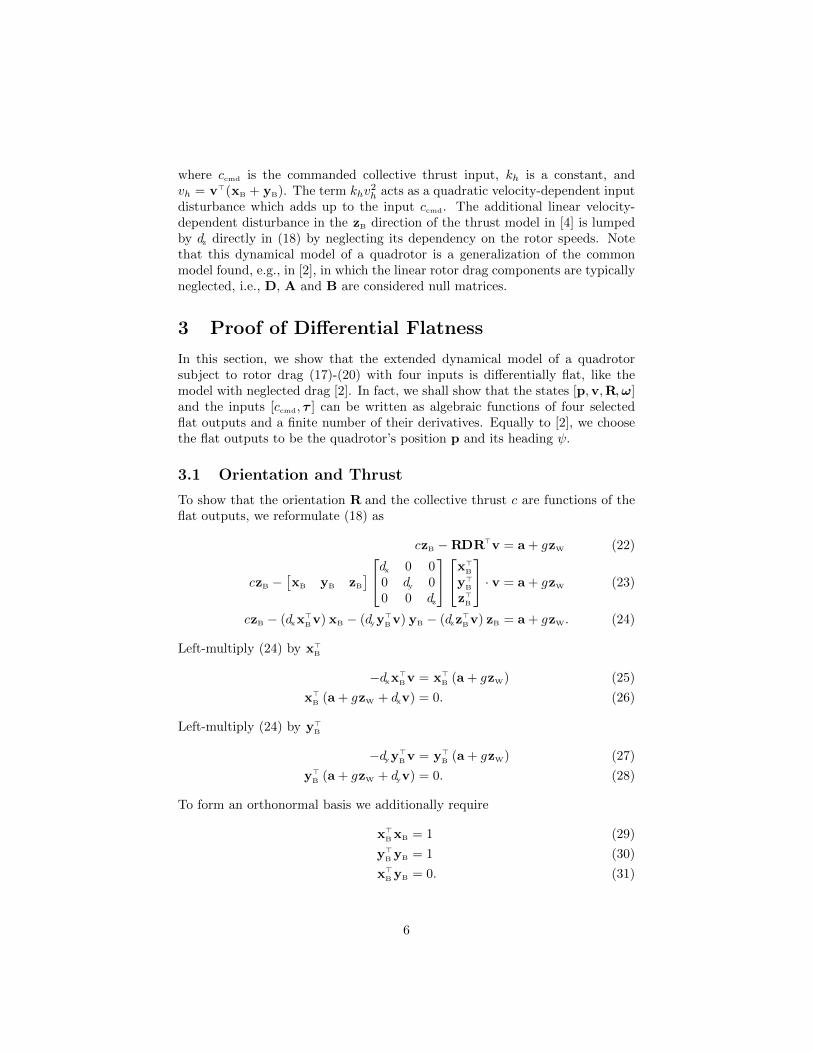
In this section, we show that the extended dynamicalmodel of a quadrotor subject to rotor drag (1)-(4) with fourinputs is differentially flat, like the model with neglecteddrag [2]. In fact, we shall show that the states [p,v,R,ω]and the inputs [ccmd, τ ] can be written as algebraic functionsof four selected flat outputs and a finite number of theirderivatives. Equally to [2], we choose the flat outputs to bethe quadrotor’s position p and its heading ψ.

To show that the orientation R and the collective thrust care functions of the flat outputs, we reformulate (2) as

czB − (dxx>Bv) xB − (dyy

>Bv) yB − (dzz

>Bv) zB

− a− gzW = 0. (6)

From left-multiplying (6) by x>B we get

x>Bα = 0, with α = a+ gzW + dxv. (7)

From left-multiplying (6) by y>B we get

y>Bβ = 0, with β = a+ gzW + dyv. (8)

To enforce a reference heading ψ, we constrain the projectionof the xB axis into the xW − yW plane to be collinear withxC (cf. Fig. 2), where

xC =[cos(ψ) sin(ψ) 0

]>(9)

yC =[− sin(ψ) cos(ψ) 0

]>. (10)

From this, (7) and (8), and the constraints that xB, yB, andzB must be orthogonal to each other and of unit length, wecan construct R with

xB =yC ×α‖yC ×α‖

(11)

yB =β × xB

‖β × xB‖(12)

zB = xB × yB. (13)

One can verify that these vectors are of unit length, perpen-dicular to each other, and satisfy the constraints (7) - (10).To get the collective thrust, we left-multiply (6) by z>

B

c = z>B (a+ gzW + dzv) . (14)

Then the collective thrust input can be computed as afunction of c, R, and the flat outputs, as

ccmd = c− kh(v>(xB + yB))2. (15)

To show that the body rates ω are functions of the flat outputsand their derivatives, we take the derivative of (2)

j = czB + cRωez −R((ωD+Dω>)R>v +DR>a) .(16)

Left-multiplying (16) by x>B and rearranging terms, we get

ωy (c− (dz − dx) (z>Bv))− ωz (dx − dy) (y>

Bv)

= x>B j+ dxx

>Ba. (17)

Left-multiplying (16) by y>B and rearranging terms, we get

ωx (c+ (dy − dz) (z>Bv)) + ωz (dx − dy) (x>

Bv)

= −y>B j− dyy>

Ba. (18)

To get a third constraint for the body rates, we project (3)along yB

ωz = y>B xB. (19)

Since xB is perpendicular to yC and zB, we can write

xB =xB

‖xB‖, with xB = yC × zB. (20)

Taking its derivative as the general derivative of a normalizedvector, we get

xB =˙xB

‖xB‖− xB

x>B˙xB

‖xB‖3(21)

and, since xB is collinear to xB and therefore perpendicularto yB, we can write (19) as

ωz = y>B

˙xB

‖xB‖. (22)

The derivative of xB can be computed as

˙xB = yC × zB + yC × zB, (23)

=(−ψxC

)× zB + yC × (ωyxB − ωxyB) . (24)

From this, (20), (22), and the vector triple product a>(b ×c) = −b>(a× c) we then get

ωz =1

‖yC × zB‖(ψx>

CxB + ωyy>C zB

). (25)

The body rates can now be obtained by solving the linearsystem of equations composed of (17), (18), and (25).

To compute the angular accelerations ω as functions ofthe flat outputs and their derivatives, we take the derivativeof (17), (18), and (25) to get a similar linear system ofequations as

ωy (c− (dz − dx) (z>Bv))− ωz (dx − dy) (y>

Bv)

= x>Bs− 2cωy − cωxωz + x>

Bξ (26)ωx (c+ (dy − dz) (z>

Bv)) + ωz (dx − dy) (x>Bv)

= −y>B s− 2cωx + cωyωz − y>

Bξ (27)−ωyy

>C zB + ωz ‖yC × zB‖= ψx>

CxB + 2ψωzx>CyB − 2ψωyx

>C zB

− ωxωyy>CyB − ωxωzy

>C zB (28)

which we can solve for ω with

c = z>B j+ ωx (dy − dz) (y>

Bv)

+ ωy (dz − dx) (x>Bv) + dzz

>Ba (29)

ξ = R(ω2D+Dω2 + 2ωDω>)R>v

+ 2R(ωD+Dω>)R>a +RDR>j. (30)

Once we know the angular accelerations, we can solve (4)for the torque inputs τ .

Note that, besides quadrotors, this proof also applies tomulti-rotor vehicles with parallel rotor axes in general. Moredetails of this proof can be found in our technical report [14].

V. CONTROL LAW

To track a reference trajectory, we use a controller con-sisting of feedback terms computed from tracking errors aswell as feed-forward terms computed from the referencetrajectory using the quadrotor’s differential flatness property.Apart from special cases, the control architectures of typicalquadrotors do not allow to apply the torque inputs directly.They instead provide a low-level body-rate controller, whichaccepts desired body rates. In order to account for this pos-sibility, we designed our control algorithm with a classicalcascaded structure, i.e., consisting of a high-level positioncontroller and the low-level body-rate controller. The high-level position controller computes the desired orientationRdes, the collective thrust input ccmd, the desired body rates

ωdes, and the desired angular accelerations ωdes, which arethen applied in a low-level controller (e.g. as presentedin [15]). As a first step in the position controller, we computethe desired acceleration of the quadrotor’s body as

ades = afb + aref − ard + gzW (31)

where afb are the PD feedback-control terms computed fromthe position and velocity control errors as

afb = −Kpos (p− pref)− Kvel (v − vref) (32)

where Kpos and Kvel are constant diagonal matrices andard = −RrefDR>

refvref are the accelerations due to rotordrag. We compute the desired orientation Rdes such that thedesired acceleration ades and the reference heading ψref isrespected as

zB,des =ades

‖ades‖(33)

xB,des =yC × zB,des

‖yC × zB,des‖(34)

yB,des = zB,des × xB,des. (35)

By projecting the desired accelerations onto the actual bodyz-axis and considering the thrust model (5), we can thencompute the collective thrust input as

ccmd = a>deszB − kh(v>(xB + yB))

2. (36)

Similarly, we can compute the desired body rates as

ωdes = ωfb + ωref (37)

where ωfb are the feedback terms computed from an at-titude controller (e.g. as presented in [16]) and ωref arefeed-forward terms from the reference trajectory, which arecomputed as described in Section IV. Finally, the desiredangular accelerations are the reference angular accelerations

ωdes = ωref (38)

which are computed from the reference trajectory as de-scribed in Section IV.

VI. DRAG COEFFICIENTS ESTIMATION

To apply the presented control law with inputs [ccmd,ω],we need to identify D, and kh, which are used to computethe reference inputs and the thrust command. If instead oneis using a platform that is controlled by the inputs [ccmd, τ ],A and B also need to be identified for computing the torqueinput. While D and kh can be accurately estimated frommeasured accelerations and velocities through (2) and (5),the effects of A and B on the body-rate dynamics (4) areweaker and require to differentiate the gyro measurements aswell as knowing the rotor speeds and rotor inertia to computeτ and τ g. Therefore, we propose to identify D, A, B, andkh by running a Nelder-Mead gradient free optimization [17]for which the quadrotor repeats a predefined trajectory ineach iteration of the optimization. During this procedure, wecontrol the quadrotor by the proposed control scheme withdifferent drag coefficients in each iteration during which we

record the absolute trajectory tracking error (39) and useit as cost for the optimization. Once the optimization hasconverged, we know the coefficients that reduce the trajectorytracking error the most. We found that the obtained values forD agree with an estimation through (2) when recording IMUmeasurements and ground truth velocity. This procedure hasthe advantage that no IMU and rotor speed measurementsare required, which are both unavailable on our quadrotorplatform used for the presented experiments, and the gyromeasurements do not need to be differentiated. This is not thecase when performing the identification through (2), (4), and(5). Also, since our method does not rely explicitly on (2), itcan also capture first order approximations of non modeledeffects lumped into the identified coefficients. Furthermore,our implementation allows stopping and restarting the opti-mization at any time, which allows changing the battery.

VII. EXPERIMENTS

A. Experimental Setup

Our quadrotor platform is built from off-the-shelf compo-nents used for first-person-view racing (see Fig. 1). It featuresa carbon frame with stiff six inch propellers, a RaceflightRevolt flight controller, an Odroid XU4 single board com-puter, and a Laird RM024 radio module for receiving controlcommands. The platform weights 610 g and has a thrust-to-weight ratio of 4. To improve its trajectory tracking accuracywe compensate the thrust commands for the varying batteryvoltage. All the presented flight experiments were conductedin an OptiTrack motion capture system to acquire the groundtruth state of the quadrotor which is obtained at 200Hz andis used for control and evaluation of the trajectory trackingperformance. Note that our control method and the rotor-dragcoefficient identification also work with state estimates thatare obtained differently than with a motion capture system.We compensate for an average latency of the perception andcontrol pipeline of 32ms. The high-level control runs on alaptop computer at 55Hz, sending collective thrust and bodyrate commands to the on-board flight controller where theyare tracked by a PD controller running at 4 kHz.

To evaluate the trajectory tracking performance and ascost for estimating the drag coefficients, we use the absolutetrajectory tracking error defined as the root mean squareposition error

Ea =

√√√√ 1

N

N∑k=1

∥∥Ekp

∥∥2, where Ekp = pk − pk

ref (39)

over N control cycles of the high-level controller requiredto execute a given trajectory.

B. Trajectories

For identifying the rotor-drag coefficients and for demon-strating the trajectory tracking performance of the proposedcontroller, we let the quadrotor execute a horizontal circletrajectory and a horizontal Gerono lemniscate trajectory.

Iteration [-]

DragCoeffi

cient[s

−1]

0 10 20 30 40 50 60 70 800.2

0.25

0.3

0.35

0.4

0.45

0.5

0.55

0.6

Fig. 3: The best performing drag coefficients dx and dy for everyiteration of the identification on both the circle and the lemniscatetrajectory.

The circle trajectory has a radius of 1.8m with a ve-locity of 4m s−1 resulting, for the case of not consider-ing rotor drag, in a required collective mass-normalizedthrust of c = 13.24m s−2 and a maximum body rates normof ‖ω‖ = 85 ◦ s−1. Its maximum nominal velocity in thexB and yB is 4.0m s−1 and 0.0m s−1 in the zB di-rection. The Gerono lemniscate trajectory is defined by[x(t) = 2 cos

(√2t); y(t) = 2 sin

(√2t)cos(√

2t)]

with amaximum velocity of 4m s−1, a maximum collective mass-normalized thrust of c = 12.98m s−2, and a maximum bodyrates norm of ‖ω‖ = 136 ◦ s−1. Its maximum nominal ve-locity in the xB and yB is 2.8m s−1 and 1.3m s−1 in thezB direction for the case of not considering rotor drag.

C. Drag Coefficients Identification

To identify the drag coefficients in D, we ran the opti-mization presented in Section VI multiple times on both thecircle and lemniscate trajectories until it converged, i.e., untilthe changes of each coefficient in one iteration is below aspecified threshold. We do not identify A and B since thequadrotor platform used for the presented experiments takes[ccmd,ω] as inputs and we therefore do not need to computethe torque inputs involving A and B according to (4). Sincewe found that dz and kh only have minor effects on thetrajectory tracking performance, we isolate the effects of dxand dy by setting dz = 0 and kh = 0 for the presented exper-iments. For each iteration of the optimization, the quadrotorflies two loops of either trajectory. The optimization typicallyconverges after about 70 iterations, which take around 30minincluding multiple battery swaps.

The evolution of the best performing drag coefficients isshown in Fig. 3 for every iteration of the proposed optimiza-tion. On the circle trajectory, we obtained dx = 0.544 s−1

and dy = 0.386 s−1, whereas on the lemniscate trajectorywe obtained dx = 0.491 s−1 and dy = 0.236 s−1. For bothtrajectories, dx is larger than dy, which is expected becausewe use a quadrotor that is wider than long. The obtained drag

x [m]

y[m

]

−2 −1.5 −1 −0.5 0 0.5 1 1.5 2

−1.5

−1

−0.5

0

0.5

1

1.5

Fig. 4: Ground truth position for ten loops on the circle trajectorywithout considering rotor drag (solid blue), with drag coefficientsestimated on the circle trajectory (solid red), and with drag co-efficients estimated on the lemniscate trajectory (solid yellow)compared to the reference position (dashed black).

coefficients identified on the circle are different than the onesidentified on the lemniscate, which is due to the fact that thecircle trajectory excites velocities in the xB and yB morethan the lemniscate trajectory. We could verify this claimby running the identification on the circle trajectory witha speed of 2.8m s−1, which corresponds to the maximumspeeds reached in xB and yB on the lemniscate trajectory. Forthis speed, we obtained dx = 0.425 s−1, and dy = 0.256 s−1

on the circle trajectory, which are close to the coefficientsidentified on the lemniscate trajectory. Additionally, in ourdynamical model, we assume the rotor drag to be indepen-dent of the thrust. This is not true in reality and thereforeleads to different results of the drag coefficient estimationon different trajectories where different thrusts are applied.These reasons suggest to carefully select a trajectory for theidentification, which goes towards the problem of finding theoptimal trajectory for parameter estimation, which is outsidethe scope of this paper. In all the conducted experiments,we found that a non zero drag coefficient in the z-directiondz does not improve the trajectory tracking performance. Wefound this to be true even for purely vertical trajectories withvelocities of up to 2.5m s−1. Furthermore, we found that anestimated kh = 0.009m−1 improves the trajectory trackingperformance further but by about one order of magnitudeless than dx and dy on the considered trajectories.

D. Trajectory Tracking Performance

To demonstrate the trajectory tracking performance of theproposed control scheme, we compare the position error ofour quadrotor flying the circle and the lemniscate trajectorydescribed above for three conditions: (i) without consideringrotor drag, (ii) with the drag coefficients estimated on thecircle trajectory, and (iii) with the drag coefficients estimatedon the lemniscate trajectory.1 Fig. 4 shows the ground truth

1Video of the experiments: https://youtu.be/VIQILwcM5PA

x [m]

y[m

]

−1.5 −1 −0.5 0 0.5 1 1.5

−1.5

−1

−0.5

0

0.5

1

1.5

Fig. 5: Ground truth position for ten loops on the lemniscatetrajectory without considering rotor drag (solid blue), with dragcoefficients estimated on the circle trajectory (solid red), andwith drag coefficients estimated on the lemniscate trajectory (solidyellow) compared to the reference position (dashed black).

and reference position when flying the circle trajectory underthese three conditions. Equally, Fig. 5 shows the groundtruth and reference position when flying the lemniscatetrajectory under the same three conditions. The trackingperformance statistics for both trajectories are summarizedin Table I. From these statistics, we see that the trajec-tory tracking performance has improved significantly whenconsidering rotor drag on both trajectories independently ofwhich trajectory the rotor-drag coefficients were estimatedon. This confirms that our approach is applicable to anyfeasible trajectory once the drag coefficients are identified,which is an advantage over methods that improve trackingperformance for a specific trajectory only (e.g. [18]). Withthe rotor-drag coefficients estimated on the circle trajectory,we achieve almost the same performance in terms of absolutetrajectory tracking error on the lemniscate trajectory as withthe coefficients identified on the lemniscate trajectory but notvice versa. As discussed above, this is due to a higher excita-tion in body velocities on the circle trajectory which resultsin a better identification of the rotor-drag coefficients. Thissuggests to perform the rotor-drag coefficients identificationon a trajectory that maximally excites the body velocities.

Since the rotor drag is a function of the velocity of thequadrotor, we show the benefits of our control approach bylinearly ramping up the maximum speed on both trajectoriesfrom 0m s−1 to 5m s−1 in 30 s. Fig. 6, and Fig. 7 show theposition error norm and the reference speed over time untilthe desired maximum speed of 5m s−1 is reached for thecircle and the lemniscate trajectory, respectively. Both figuresshow that considering rotor drag does not improve trajectorytracking for small speeds below 0.5m s−1 but noticeablydoes so for higher speeds.

An analysis of the remaining position error for the casewhere rotor drag is considered reveals that it strongly corre-lates to the applied collective thrust. In the used dynamical

Time [s]

PositionErrorNorm

‖Ep‖[m

]

Speed[ms]

0 5 10 15 20 25 300

0.1

0.2

0.3

0.4

0.5

0

1

2

3

4

5

Fig. 6: Position error norm ‖Ep‖ when ramping the speed onthe circle trajectory from 0m s−1 up to 5m s−1 in 30 s withoutconsidering rotor drag (solid blue), with drag coefficients estimatedon the circle trajectory (solid red), and with drag coefficientsestimated on the lemniscate trajectory (solid yellow). The referencespeed on the trajectory is shown in dashed purple.

model of a quadrotor, we assume the rotor drag to beindependent of the thrust [c.f. (2)], which is not true inreality. For the experiment in Fig. 6, the commanded mass-normalized collective thrust varies between 10m s−2 and18m s−2 which clearly violates the constant thrust assump-tion. By considering a dependency of the rotor drag on thethrust might improve trajectory tracking even further and issubject of future work.

VIII. COMPARISON TO OTHER CONTROL METHODS

In this section, we present a qualitative comparison toother quadrotor controllers that consider rotor drag effectsas presented in [10], [11], [12], and [13].

None of these works show or exploit the differentialflatness property of quadrotor dynamics subject to rotor drageffects. They also do not consider asymmetric vehicles wheredx 6= dy and they omit the computation of ωz and ωz .

In [10] and [11], the presented position controller de-composes the rotor drag force into a component that isindependent of the vehicle’s orientation and one along thethrust direction, which leads to an explicit expression for the

TABLE I: Maximum and standard deviation of the position errorEp as well as the absolute trajectory tracking error Ea (39) overten loops on both the circle and the lemniscate trajectory. For eachtrajectory, we perform the experiment without considering drag,with the drag coefficients identified on the circle trajectory, andwith the drag coefficients identified on the lemniscate trajectory.

Trajectory Params ID max (‖Ep‖) σ (‖Ep‖) Ea

[cm] [cm] [cm]

CircleNot Cons. Drag 21.08 2.11 17.53

Circle 14.54 2.63 6.54Lemniscate 12.39 2.53 8.16

LemniscateNot Cons. Drag 16.79 3.19 11.27

Circle 10.25 2.30 5.56Lemniscate 10.02 2.23 5.51

Time [s]

PositionErrorNorm

‖Ep‖[m

]

Speed[ms]

0 5 10 15 20 25 300

0.05

0.1

0.15

0.2

0

1

2

3

4

5

Fig. 7: Position error norm ‖Ep‖ when ramping the maximumspeed on the lemniscate trajectory from 0m s−1 up to 5m s−1 in30 s without considering rotor drag (solid blue), with drag coeffi-cients estimated on the circle trajectory (solid red), and with dragcoefficients estimated on the lemniscate trajectory (solid yellow).The reference speed on the trajectory is shown in dashed purple.

desired thrust direction. They both neglect feed-forward onangular accelerations, which does not allow perfect trajectorytracking. As in our work, [10] models the rotor drag tobe proportional to the square root of the thrust, whichis proportional to the rotor speed, but then assumes thethrust to be constant for the computation of the rotor drag,whereas [11] models the rotor drag to be proportional to thethrust. Simulation results are presented in [10] while realexperiments with speeds of up to 2.5m s−1 were conductedin [11].

The controller in [12] considers rotor drag in the com-putation of the thrust command and the desired orientationbut it does not use feed-forward terms on body rates andangular accelerations, which does not allow perfect trajectorytracking. In our work, we use the same thrust model butneglect its dependency on the rotor speed. In [12], alsothe rotor drag is modeled to depend on the rotor speed,which is physically correct but requires the rotor speedsto be measured for it to be considered in the controller.They present real experiments with speeds of up to 4.0m s−1

and unlike us also show trajectory tracking improvements invertical flight.

As in our work, [13] considers rotor drag for the computa-tion of the desired thrust, orientation, body rates, and angularaccelerations. However, their computations rely on a modelwhere the rotor drag is proportional to the rotor thrust. Also,they neglect the snap of the trajectory and instead requirethe estimated acceleration and jerk, which are typically notavailable, for computing the desired body rates and angularaccelerations. The presented results in [13] stem from realexperiments with speeds of up to 1.0m s−1.

IX. CONCLUSION

We proved that the dynamical model of a quadrotor subjectto linear rotor drag effects is differentially flat. This property

was exploited to compute feed-forward control terms asalgebraic functions of a reference trajectory to be tracked. Wepresented a control policy that uses these feed-forward terms,which compensates for rotor drag effects, and thereforeimproves the trajectory tracking performance of a quadrotoralready from speeds of 0.5m s−1 onwards. The proposedcontrol method reduces the root mean squared tracking errorby 50% independently of the executed trajectory, which weshowed by evaluating the tracking performance of a circleand a lemniscate trajectory. In future work, we want toconsider the dependency of the rotor drag on the appliedthrust to further improve the trajectory tracking performanceof quadrotors.

REFERENCES

[1] M. Burri, M. Bloesch, Z. Taylor, R. Siegwart, and J. Nieto, “Aframework for maximum likelihood parameter identification appliedon MAVs,” J. Field Robot., pp. 1–18, June 2017.

[2] D. Mellinger and V. Kumar, “Minimum snap trajectory generation andcontrol for quadrotors,” in IEEE Int. Conf. Robot. Autom. (ICRA), May2011, pp. 2520–2525.

[3] J. Ferrin, R. Leishman, R. Beard, and T. McLain, “Differential flatnessbased control of a rotorcraft for aggressive maneuvers,” in IEEE/RSJInt. Conf. Intell. Robot. Syst. (IROS), Sept. 2011, pp. 2688–2693.

[4] P. J. Bristeau, P. Martin, E. Salaun, and N. Petit, “The role of propelleraerodynamics in the model of a quadrotor UAV,” in IEEE Eur. ControlConf. (ECC), Aug. 2009, pp. 683–688.

[5] P. Martin and E. Salaun, “The true role of accelerometer feedbackin quadrotor control,” in IEEE Int. Conf. Robot. Autom. (ICRA), May2010, pp. 1623–1629.

[6] R. Mahony, V. Kumar, and P. Corke, “Multirotor aerial vehicles:Modeling, estimation, and control of quadrotor,” IEEE Robot. Autom.Mag., vol. 19, no. 3, pp. 20–32, 2012.

[7] R. C. Leishman, J. C. Macdonald, R. W. Beard, and T. W. McLain,“Quadrotors and accelerometers: State estimation with an improveddynamic model,” Control Systems, IEEE, vol. 34, no. 1, pp. 28–41,Feb. 2014.

[8] M. Burri, M. Datwiler, M. W. Achtelik, and R. Siegwart, “Robuststate estimation for micro aerial vehicles based on system dynamics,”in IEEE Int. Conf. Robot. Autom. (ICRA), 2015, pp. 5278–5283.

[9] M. Bangura and R. Mahony, “Thrust control for multirotor aerialvehicles,” IEEE Trans. Robot., vol. 33, no. 2, pp. 390–405, Apr. 2017.

[10] J.-M. Kai, G. Allibert, M.-D. Hua, and T. Hamel, “Nonlinear feedbackcontrol of quadrotors exploiting first-order drag effects,” in IFAC WorldCongress, vol. 50, no. 1, July 2017, pp. 8189–8195.

[11] S. Omari, M.-D. Hua, G. Ducard, and T. Hamel, “Nonlinear controlof VTOL UAVs incorporating flapping dynamics,” in IEEE/RSJ Int.Conf. Intell. Robot. Syst. (IROS), Nov. 2013, pp. 2419–2425.

[12] J. Svacha, K. Mohta, and V. Kumar, “Improving quadrotor trajectorytracking by compensating for aerodynamic effects,” in IEEE Int. Conf.Unmanned Aircraft Syst. (ICUAS), June 2017, pp. 860–866.

[13] M. Bangura, “Aerodynamics and control of quadrotors,” Ph.D. disser-tation, College of Engineering and Computer Science, The AustralianNational University, 2017.

[14] M. Faessler, A. Franchi, and D. Scaramuzza, “Detailed derivationsof ‘Differential flatness of quadrotor dynamics subject to rotor dragfor accurate tracking of high-speed trajectories’,” arXiv e-prints, Dec.2017. [Online]. Available: http://arxiv.org/abs/1712.02402

[15] M. Faessler, D. Falanga, and D. Scaramuzza, “Thrust mixing, satura-tion, and body-rate control for accurate aggressive quadrotor flight,”IEEE Robot. Autom. Lett., vol. 2, no. 2, pp. 476–482, Apr. 2017.

[16] M. Faessler, F. Fontana, C. Forster, and D. Scaramuzza, “Automaticre-initialization and failure recovery for aggressive flight with amonocular vision-based quadrotor,” in IEEE Int. Conf. Robot. Autom.(ICRA), 2015, pp. 1722–1729.

[17] J. A. Nelder and R. Mead, “A simplex method for function minimiza-tion,” The Computer Journal, vol. 7, no. 4, pp. 308–313, Jan. 1965.

[18] M. Hehn and R. D’Andrea, “A frequency domain iterative learningalgorithm for high-performance, periodic quadrocopter maneuvers,” J.Mechatronics, vol. 24, no. 8, pp. 954–965, 2014.

Detailed Derivations of ”Differential Flatness of

Quadrotor Dynamics Subject to Rotor Drag for

Accurate Tracking of High-Speed Trajectories”

Matthias Faessler, Antonio Franchi, and Davide Scaramuzza

Abstract

This technical report provides detailed intermediate steps of the proofof differential flatness of quadrotor dynamics subject to rotor drag effectspresented in [1]. It also shows how we handle singularities that arisefrom this math for certain states related to free fall of the quadrotor.Furthermore, it explains incorrectnesses in the proof of differential flatnessof quadrotor dynamics without rotor drag presented in [2] which might beconfusing when comparing the two works.

How to Cite this Work

This technical report is accompanying our IEEE Robotics and Automation Let-ters paper [1]. If you wish to reference this work, please cite this paper asfollows:

@Article{Faessler 18ral ,

author = {Matthias Faessler and Antonio Franchi

and Davide Scaramuzza},

title = {Differential Flatness of Quadrotor Dynamics

Subject to Rotor Drag for Accurate ,

High -Speed Trajectory Tracking},

journal = {{IEEE} Robot. Autom. Lett.},

year = 2018,

volume = 3,

number = 2,

pages = {620--626},

month = apr ,

doi = {10.1109/ LRA .2017.2776353} ,

issn = {2377 -3766}

}

1

Contents

1 Math Basics 31.1 Definitions and Nomenclature . . . . . . . . . . . . . . . . . . . . 31.2 Some Useful Identities and Derivations . . . . . . . . . . . . . . . 41.3 Vector Derivatives in Different Coordinate Frames . . . . . . . . 4

2 Dynamical Model 5

3 Proof of Differential Flatness 63.1 Orientation and Thrust . . . . . . . . . . . . . . . . . . . . . . . 63.2 Body Rates . . . . . . . . . . . . . . . . . . . . . . . . . . . . . . 73.3 Torque Inputs . . . . . . . . . . . . . . . . . . . . . . . . . . . . . 9

4 Special Cases 11

Appendices 14

A Incorrectnesses in Original Differential Flatness Derivation 14

2

xB

yB

zB

Body

xW

yW

zW = zC

World

xC

yC

ψ

−gzW

Figure 1: Schematics of the considered quadrotor model with the used coordinatesystems.

1 Math Basics

1.1 Definitions and Nomenclature

In this work, we make use of a world frameW with orthonormal basis {xW, yW, zW}represented in world coordinates and a body frame B with orthonormal basis{xB, yB, zB} also represented in world coordinates. The body frame is fixedto the quadrotor with an origin coinciding with its center of mass as depictedin Fig. 1. The quadrotor is subject to a gravitational acceleration g in neg-ative zW direction. We denote the position of the quadrotor’s center of massas p, and its derivatives, velocity, acceleration, jerk, and snap as v, a, j, ands, respectively. We represent the quadrotor’s orientation as a rotation matrixR =

[xB yB zB

]and its body rates (i.e., the angular velocity) as ω repre-

sented in body coordinates. In this work, we often make use of a skew symmetricmatrix formed from the body rates which is defined by

ω =

0 −ωz ωy

ωz 0 −ωx

−ωy ωx 0

. (1)

We define a rotor drag matrix, which is a constant diagonal matrix composedof the rotor drag coefficients, as

D =

dx 0 00 dy 00 0 dz

. (2)

3

To denote unit vectors along the coordinate axes we use

ex =[1 0 0

]>(3)

ey =[0 1 0

]>(4)

ez =[0 0 1

]>. (5)

Finally, we denote quantities that can be computed from a reference trajectoryas reference values and quantities that are computed by an outer loop feedbackcontrol law and passed to an inner loop controller as desired values.

1.2 Some Useful Identities and Derivations

The skew symmetric matrix ω has the following properties:

ω> = −ω (6)

ω> · b = −ω · b = −ω × b = b× ω (7)

where b is an arbitrary vector. The derivative of the orientation is

R = R · ω (8)

and the derivative of the norm of a vector b can be written as

d

dt‖b‖ =

b> · b‖b‖ . (9)

Finally, in this work, we make use of the vector triple product of arbitraryvectors a, b, and c:

a>(b× c) = −b>(a× c). (10)

1.3 Vector Derivatives in Different Coordinate Frames

Since derivatives of vectors that are represented in different coordinate framesare important for the derivations in the proof of differential flatness of quadrotordynamics, we introduce them here in detail. To avoid confusion in this section,unlike in the rest of this report, we use subscripts to explicitly denote whateach variable depicts and in which coordinates it is represented. We denote thederivative of an arbitrary vector b which is then represented in a coordinateframe A as A

˙(b) and the pure element wise derivative as Ab.Since the world frame W is an inertial frame, taking the derivative of a

vector represented in world coordinates corresponds to taking the element wisederivative

W˙(b) = Wb. (11)

A vector represented in world coordinates Wb is related to its representation inbody coordinates Bb by a rotation RWB that represents the orientation of thebody frame B with respect to the world frame W as

Wb = RWB · Bb. (12)

4

With this and (8), we can write (11) as

W˙(b) = Wb = RWB · Bb + RWB · BωWB · Bb. (13)

Transforming this into body coordinates results in

B˙(b) = R>

WB · W ˙(b) = Bb + BωWB × Bb. (14)

In this work, we often make use of derivatives of the basis vectors of the bodyframe xB, yB, and zB. Since these vectors are constant when represented inbody coordinates their element wise derivative in body coordinates is zero (e.g.,

BxB = 0). Therefore, we get the derivative of e.g. xB represented in world andbody coordinates as

W˙(xB) = RWB · BωWB · BxB (15)

B˙(xB) = BωWB · BxB = BωWB × BxB. (16)

Since we almost exclusively represent vectors in world coordinates and the ele-ment wise derivative of the basis vectors are zero, we will write the derivativeof a basis vector represented in world coordinates as xB instead of W

˙(xB), as itis done in [1], for clarity in the remainder of this report.

Note that a confusion of derivatives of vectors represented in world coordi-nates or in body coordinates led to mistakes in [2], which we describe in moredetail in Appendix A.

2 Dynamical Model

We consider the dynamical model of a quadrotor with rotor drag developedin [3] with no wind, stiff propellers, and no dependence of the rotor drag on thethrust. According to this model, the dynamics of the position p, velocity v,orientation R, and body rates ω can be written as

p = v (17)

v = −gzW + czB −RDR>v (18)

R = Rω (19)

ω = J−1 (τ − ω × Jω − τ g −AR>v −Bω) (20)

where c is the mass-normalized collective thrust, D = diag (dx, dy, dz) is a con-stant diagonal matrix formed by the mass-normalized rotor-drag coefficients, ωis a skew-symmetric matrix formed from ω, J is the quadrotor’s inertia matrix,τ is the three dimensional torque input, τ g are gyroscopic torques from thepropellers, and A and B are constant matrices. For the derivations and moredetails about these terms, please refer to [3]. In this work, we adopt the thrustmodel presented in [4]

c = ccmd + khv2h (21)

5

where ccmd is the commanded collective thrust input, kh is a constant, andvh = v>(xB + yB). The term khv

2h acts as a quadratic velocity-dependent input

disturbance which adds up to the input ccmd. The additional linear velocity-dependent disturbance in the zB direction of the thrust model in [4] is lumpedby dz directly in (18) by neglecting its dependency on the rotor speeds. Notethat this dynamical model of a quadrotor is a generalization of the commonmodel found, e.g., in [2], in which the linear rotor drag components are typicallyneglected, i.e., D, A and B are considered null matrices.

3 Proof of Differential Flatness

In this section, we show that the extended dynamical model of a quadrotorsubject to rotor drag (17)-(20) with four inputs is differentially flat, like themodel with neglected drag [2]. In fact, we shall show that the states [p,v,R,ω]and the inputs [ccmd, τ ] can be written as algebraic functions of four selectedflat outputs and a finite number of their derivatives. Equally to [2], we choosethe flat outputs to be the quadrotor’s position p and its heading ψ.

3.1 Orientation and Thrust

To show that the orientation R and the collective thrust c are functions of theflat outputs, we reformulate (18) as

czB −RDR>v = a + gzW (22)

czB −[xB yB zB

] dx 0 00 dy 00 0 dz

x>B

y>B

z>B

· v = a + gzW (23)

czB − (dxx>Bv) xB − (dyy>

Bv) yB − (dzz>Bv) zB = a + gzW. (24)

Left-multiply (24) by x>B

−dxx>Bv = x>

B (a + gzW) (25)

x>B (a + gzW + dxv) = 0. (26)

Left-multiply (24) by y>B

−dyy>Bv = y>

B (a + gzW) (27)

y>B (a + gzW + dyv) = 0. (28)

To form an orthonormal basis we additionally require

x>B xB = 1 (29)

y>B yB = 1 (30)

x>B yB = 0. (31)

6

To enforce a reference heading ψ, we constrain the projection of the xB axis intothe xW − yW plane to be collinear with xC (c.f. Fig 1), where

xC =[cos(ψ) sin(ψ) 0

]>(32)

yC =[− sin(ψ) cos(ψ) 0

]>. (33)

From these constraints we can construct R with

xB =yC ×α‖yC ×α‖

(34)

yB =β × xB

‖β × xB‖(35)

zB = xB × yB (36)

asR =

[xB yB zB

](37)

where

α = a + gzW + dxv (38)

β = a + gzW + dyv. (39)

One can verify that these vectors are of unit length, perpendicular to eachother, and satisfy the constraints (26) - (33). To get the thrust input, we left-multiply (24) by z>

B

c− dzz>Bv = z>

B (a + gzW) (40)

c = z>B (a + gzW + dzv) . (41)

Then the collective thrust input can be computed as a function of c, R, and theflat outputs, according to the thrust model (21) as

ccmd = c− kh(v>(xB + yB))2. (42)

3.2 Body Rates

To show that the body rates ω are functions of the flat outputs and theirderivatives, we take the derivative of (18)

j = czB + cRωez −R((ωD + Dω>) R>v + DR>a) . (43)

Left multiply (43) by x>B

x>B j = cωy − ωz (dx − dy) (y>

Bv)− ωy (dz − dx) (z>Bv)− dxx>

Ba. (44)

Left multiply (43) by y>B

y>B j = −cωx − ωz (dx − dy) (x>

Bv)− ωx (dy − dz) (z>Bv)− dyy>

Ba. (45)

7

By projecting (19) along the yB we get

y>B R = y>

BRω (46)

ωz = y>B xB. (47)

Since xB is perpendicular to yC and zB, we can write

xB =xB

‖xB‖, with xB = yC × zB. (48)

Taking its derivative as the general derivative of a normalized vector, we get

xB =˙xB

‖xB‖− xB

x>B

˙xB

‖xB‖3. (49)

Since xB is collinear to xB and therefore perpendicular to yB, we can write (47)as

ωz = y>B

˙xB

‖xB‖. (50)

The derivative of xB can be computed as

˙xB = yC × zB + yC × zB (51)

where, using (15),

yC = RWC

(ψez × ey

)(52)

=[xC yC zC

] (−ψex

)(53)

= −ψxC (54)

and

zB = Rωez (55)

= R

ωy

−ωx

0

(56)

= ωyxB − ωxyB (57)

and therefore

˙xB = −ψxC × zB + ωyyC × xB − ωxyC × yB. (58)

8

From this and (50) and using the property in (10), we then get

ωz = y>B

˙xB

‖xB‖(59)

=1

‖xB‖(−ψy>

B (xC × zB) + ωyy>B (yC × xB)

)(60)

=1

‖xB‖(ψx>

C (yB × zB)− ωyy>C (yB × xB)

)(61)

=1

‖xB‖(ψx>

C xB + ωyy>C zB

). (62)

The body rates can then be computed from a linear system of equations com-posed of (44), (45), and (62)

ωy (c− (dz − dx) (z>Bv))− ωz (dx − dy) (y>

Bv) = x>B j + dxx

>Ba (63)

ωx (c+ (dy − dz) (z>Bv)) + ωz (dx − dy) (x>

Bv) = −y>B j− dyy>

Ba (64)

−ωyy>C zB + ωz ‖yC × zB‖ = ψx>

C xB (65)

as

ωx =−B1C2D3 + B1C3D2 − B3C1D2 + B3C2D1

A2 (B1C3 − B3C1)(66)

ωy =−C1D3 + C3D1

B1C3 − B3C1(67)

ωz =B1D3 − B3D1

B1C3 − B3C1(68)

where

B1 = c− (dz − dx) (z>Bv) (69)

C1 = − (dx − dy) (y>Bv) (70)

D1 = x>B j + dxx

>Ba (71)

A2 = c+ (dy − dz) (z>Bv) (72)

C2 = (dx − dy) (x>Bv) (73)

D2 = −y>B j− dyy>

Ba (74)

B3 = −y>C zB (75)

C3 = ‖yC × zB‖ (76)

D3 = ψx>C xB. (77)

3.3 Torque Inputs

To show that the angular accelerations ω are functions of the flat outputs andtheir derivatives, we take the derivative of (43)

s = czB + 2cRωez + c(Rω2ez + R ˙ωez

)−R

(˙ωD + D ˙ω

>)

R>v − ξ (78)

9

where

ξ = R(ω2D + Dω2 + 2ωDω>) R>v + 2R(ωD + Dω>) R>a + RDR>j. (79)

Left multiplying (78) by x>B and rearranging terms

ωyB1 + ωzC1 = x>Bs− 2cωy − cωxωz + x>

Bξ. (80)

Left multiplying (78) by y>B and rearranging terms

ωxA2 + ωzC2 = −y>B s− 2cωx + cωyωz − y>

Bξ. (81)

We get a third constraint for the angular accelerations by differentiating (65)and using (48) as

− ωyy>C zB − ωy y>

C zB − ωyy>C zB + ωz ‖yC × zB‖+ ωz

x>B

˙xB

‖xB‖= ψx>

C xB + ψx>C xB + ψx>

C xB (82)

which can be simplified to

−ωyy>C zB + ωz ‖yC × zB‖ = ψx>

C xB + 2ψωzx>C yB − 2ψωyx>

C zB

− ωxωyy>C yB − ωxωzy>

C zB (83)

by using the following derivations:From (54) we get

− ωy y>C zB = ψωyx>

C zB. (84)

From(57) and the fact that y>C xB = 0, we get

− ωyy>C zB = ωxωyy>

C yB. (85)

From (48) and using (10) and (58) we get

ωzx>

B˙xB

‖xB‖= ωzx>

B˙xB (86)

= ωzx>B

(−ψxC × zB + ωyyC × xB − ωxyC × yB

)(87)

= ωz

(−ψx>

B (xC × zB)− ωxx>B (yC × yB)

)(88)

= ωz

(ψx>

C (xB × zB) + ωxy>C (xB × yB)

)(89)

= ωz

(−ψx>

C yB + ωxy>C zB

). (90)

Similarly to (54), we can derive

xC = RWC

(ψez × ex

)(91)

=[xC yC zC

] (ψey

)(92)

= ψyC (93)

10

and with this and the fact that y>C xB = 0

ψx>C xB = ψ2y>

C xB = 0. (94)

And finally, similarly to (57), we get

xB = Rωex (95)

= R

0ωz

−ωy

(96)

= ωzyB − ωyzB (97)

which leads toψx>

C xB = ψωzx>C yB − ψωyx>

C zB. (98)

The derivative of the thrust can be obtained by left multiplying (43) by z>B

c = z>B j + ωx (dy − dz) (y>

Bv) + ωy (dz − dx) (x>Bv) + dzz

>Ba. (99)

The angular accelerations can now be computed from a linear system of equa-tions composed of (80), (81), and (83)

ωyB1 + ωzC1 = E1 (100)

ωxA2 + ωzC2 = E2 (101)

ωyB3 + ωzC3 = E3 (102)

as

ωx =−B1C2E3 + B1C3E2 − B3C1E2 + B3C2E1

A2 (B1C3 − B3C1)(103)

ωy =−C1E3 + C3E1B1C3 − B3C1

(104)

ωz =B1E3 − B3E1B1C3 − B3C1

(105)

where

E1 = x>Bs− 2cωy − cωxωz + x>

Bξ (106)

E2 = −y>B s− 2cωx + cωyωz − y>

Bξ (107)

E3 = ψx>C xB + 2ψωzx>

C yB − 2ψωyx>C zB − ωxωyy>

C yB − ωxωzy>C zB. (108)

The torque inputs can finally be computed from (20).

4 Special Cases

In this section, we present some practical workarounds for some special caseswhere the presented math is not valid. These workarounds typically only workif we can assume that these special cases only occur for very short durations ata time.

11

Case - yC ×α = 0: This case occurs if either yC is aligned with α (definedin (38)) or α = 0. In this case, any xB that is perpendicular to yC satisfies theconstraint (26). To overcome this ambiguity, we compute xB by projecting theestimated body x-axis into the xC − zC plane and normalizing it as

xB =xB,est −

(x>

B,estyC

)yC∥∥xB,est −

(x>

B,estyC

)yC

∥∥ . (109)

If the obtained∥∥xB,est −

(x>

B,estyC

)yC

∥∥ = 0, we set xB = xC. Note that thismight lead to jumps in the desired orientation. By assuming that this specialcase only occurs for a short duration it might be better to just remember thelast desired orientation that was computed before the special case occurred.

Case - β × xB = 0: This case occurs if either xB is aligned with β (definedin (39)) or β = 0. In this case, any yB that is perpendicular to xB satisfiesthe constraint (54). To overcome this ambiguity, we compute yB by the crossproduct of the estimated body z-axis zB,est and xB and normalizing it as

yB =zB,est × xB

‖zB,est × xB‖. (110)

If the obtained ‖zB,est × xB‖ = 0, we set yB = yC. Note that this might leadto jumps in the desired orientation. By assuming that this special case onlyoccurs for a short duration it might be better to just remember the last desiredorientation that was computed before the special case occurred.

Case - Inverted Flight where z>Wα < 0: In the case where z>

Wα < 0, (34)leads to a body x-axis xB which has a projection into the xW − yW plane thatpoints into the −xC direction. It is still collinear to xC but this causes theactual heading to be off by 180◦ from the reference heading ψref . Enforcing thereference heading during inverted flight by changing the sign of the desired xB

axis might lead to a jump in the desired orientation. However, to the best ofour knowledge, it is not possible to prevent jumps in the orientation for anytrajectory. For example, when performing a vertical loop where parts of it areflown upside down, we end up with a continuous orientation of the quadrotorfor a reference heading ψref = 0◦ when allowing the quadrotor to have its actualheading 180◦ off as long as it flies upside down. When doing the same with areference heading ψref = 90◦, we do not end up with a continuous orientation ofthe quadrotor when applying the same method. In this particular case, changingthe sign of xB when the quadrotor is inverted, would lead to a continuousorientation over the entire loop. In summary, the presented computation of thedesired orientation is not well suited for inverted flights, which require specialconsiderations.

Case - A2 = 0 or (B1C3 − B3C1) = 0: The solutions of the body rates (66)-(68) and angular accelerations (103)-(105) are obtained by divisions where the

12

denominator is composed of coefficients as defined in (69)-(77). These denom-inator can become zero which makes the body rates and angular accelerationsundefined. Similarly to α = 0 and β = 0, this is the case where the quadrotoris executing ballistic trajectories. In such cases we set ω = 0 and ω = 0.

13

Appendices

A Incorrectnesses in Original Differential Flat-ness Derivation

The work presented in [1] extends the work of [2], which can be considered thefirst paper that proves differential flatness for quadrotors without consideringrotor drag. However, we would like to point out two incorrectnesses found in [2]that might be confusing when comparing it to our derivations. For this, weuse red color to refer to equations in [2]. Note that in this work we are usinga different index convention, i.e., we denote the rotation rates of e.g. B withrespect to W as ωWB whereas it is denoted as ωBW in [2] but in this section, weadopt their convention when referring to their equations.

The first incorrectness in [2] is due to a confusion of the representation of vectorsin world or body coordinates (see Section 1.3 for details). In equation (7) thederivative of equation (3) is computed as

ma = u1zB + ωBW × u1zB. (111)

However, equation (3) including zB is represented in world coordinates. Bytaking its derivative, we get

ma = u1zB + u1 zB (112)

= u1zB + u1Rωez. (113)

The fallacy in (111) is that zB is computed as if zB was represented in bodycoordinates (c.f. (16)) but it is represented in world coordinates and hence itsderivative is zB = Rωez, (c.f. (15)). However, by chance, the correct roll andpitch rates are obtained in [2] since the projections of ωBW × zB and Rωez ontothe xB and yB axes are equal. Note that when taking the second derivative ofequation (3) as done in [2] and computing the angular accelerations from that,unlike for the body rates, would not result in correct values anymore.

The second incorrectness in [2] in the same section in the computation of thethird component of the body rates. It is stated that ”the third component r isfound by simply writing ωBW = ωBC + ωCW and observing that ωBC has no zB

component”, which is not correct, i.e., generally ωBC · zB 6= 0. Based on thisincorrect assumption, the third component of the body rates is then computedas

r = ωCW · zB = ψzW · zB (114)

but forωBW = ωBC + ωCW (115)

to hold, all vectors must be expressed in the same coordinate frame, whichin this case has to be the B frame since the body rates ωBW are expressed

14

in body coordinates. Conversely, ωCW = ψzW as used in (114) is only valid ifωCW was expressed in world coordinates, which is not the case. Similarly, theangular accelerations are computed incorrectly. The necessary third constraintfor computing the correct body rates is (47).

References

[1] M. Faessler, A. Franchi, and D. Scaramuzza, “Differential flatness of quadro-tor dynamics subject to rotor drag for accurate tracking of high-speed tra-jectories,” IEEE Robot. Autom. Lett., vol. 3, no. 2, pp. 620–626, Apr. 2018.

[2] D. Mellinger and V. Kumar, “Minimum snap trajectory generation and con-trol for quadrotors,” in IEEE Int. Conf. Robot. Autom. (ICRA), May 2011,pp. 2520–2525.

[3] J.-M. Kai, G. Allibert, M.-D. Hua, and T. Hamel, “Nonlinear feedbackcontrol of quadrotors exploiting first-order drag effects,” in IFAC WorldCongress, vol. 50, no. 1, July 2017, pp. 8189–8195.

[4] J. Svacha, K. Mohta, and V. Kumar, “Improving quadrotor trajectory track-ing by compensating for aerodynamic effects,” in IEEE Int. Conf. UnmannedAircraft Syst. (ICUAS), June 2017, pp. 860–866.

15