Differential Equation Models forForecasting Highway Traffic Flow

R. Eddie Wilson, University of Bristol

EPSRC Advanced Fellowship EP/E055567/1http://www.enm.bris.ac.uk/staff/rew

Differential Equation Models for Forecasting Highway Traffic Flow – p. 1/32

Outline of talk

Data part I (fairly standard)

Differential equation models

Data part II (revolutionary)

Differential Equation Models for Forecasting Highway Traffic Flow – p. 2/32

Inductance Loop Infrastructure

Loop pairs every 500m, sometimes closer

Measure lane, time, speed, vehicle length

Results usually time-averaged (1 minute)

Part of UK Highways Agency Controlled Motorwaysproject and similar systems in many other countries

Differential Equation Models for Forecasting Highway Traffic Flow – p. 3/32

Active Traffic Management

Intelligent Transport Systems on highwaysQueue Ahead warning systemsTemporary speed limitsLane managementRamp metering

Spacing of inductance loop sites is in range 30m to100m – usual operation gives 1 minute averages

Differential Equation Models for Forecasting Highway Traffic Flow – p. 4/32

Birmingham Box motorway system

������������

������������

������������

������������

J4

J5

J6

ACTI

VE T

RAFF

IC M

ANAG

EMEN

TDifferential Equation Models for Forecasting Highway Traffic Flow – p. 5/32

Patterns at a Single Detector

Data from single loop site (3 lanes active):

0 5 10 15 200

20

40

60

80

100

120

5 10 15 200

20

40

60

80

100

120

140total flowper minute(3 lanes)

time (hrs) time (hrs)

lanes 1 2 3

spee

d (k

m/h

)

Very similar pictures all over the world

No simple relation between speed and flow:consequences for system versus driver optimality

Differential Equation Models for Forecasting Highway Traffic Flow – p. 6/32

Speed-Flow Relationship

0 5 10 15 20 25 30 35 40 450

20

40

60

80

100

120

140

160

flow (vehs/min)

velo

city

(km

/h)

free flow (Poissonian statistics etc.)

congestion

vehicles interactoscillations

lane 2 records only

Differential Equation Models for Forecasting Highway Traffic Flow – p. 7/32

Speed-Density and Flow-Density

0 10 20 30 40 50 60 70 800

20

40

60

80

100

120

140

160

0 10 20 30 40 50 60 70 80 900

5

10

15

20

25

30

35

40

45velocity (km/h)

density (veh/km) density (veh/km)

flow

(ve

hs/m

in)

lane 2 measurementsonly

oscillations

free

flow

congestioncongestion

freeflow

Suggests state relationship v = V (ρ), flow = ρV (ρ)v is velocity, ρ is density

Why the high flow variation in congested conditions?To explain, need to consider spatial effects also

Differential Equation Models for Forecasting Highway Traffic Flow – p. 8/32

Spatiotemporal data from the M42

distance in km against time in hrs.

Differential Equation Models for Forecasting Highway Traffic Flow – p. 9/32

Zoom into structure

distance in km against time in hrs.

Differential Equation Models for Forecasting Highway Traffic Flow – p. 10/32

Outline of talk

Data part I (fairly standard)

Differential equation models

Data part II (revolutionary)

Differential Equation Models for Forecasting Highway Traffic Flow – p. 11/32

Some facts and conclusions

Ignition of stop-and-go waves is irregularneeds full noisiness of microscopic description (butpredictions can only be probabilistic)

Wavelength is much longer than vehicle separationhow to capture the upscaling effect?

General idea here: identify families of models which arequalitatively ok and throw away models which arequalitatively inadequate

IN FUTUREFit models to microscopic dataUse emergent macroscopic dynamics for predictions

Differential Equation Models for Forecasting Highway Traffic Flow – p. 12/32

‘Whole-link’ Models ( ≃ most macro)

General idea, travel time model:

τ = f(x(t))

τ transit time for vehicles entering link at time t

x is number of vehicles on link at time t

Conservation:x(t) = qin(t) − qout(t),

qout(t + τ(t)) =qin(t)

1 + τ(t)

Some type of neutral delay differential equation

Useless for studying spatial pattern, maybe ok fornetwork equilibrium problems

Differential Equation Models for Forecasting Highway Traffic Flow – p. 13/32

PDE Modelling Approach (I)

Work with continuous density ρ(x, t), velocity v(x, t)

Conservation of vehicles

ρt + (ρv)x = 0.

Lighthill-Whitham-Richards (LWR) 1950s

v = V (ρ) (speed-density function)

Typical choice, Greenshield’s model

V (ρ) = vmax

(

1 −ρ

ρmax

)

, (1)

gives unimodal fundamental diagram Q(ρ) := ρV (ρ),characteristics give shock-waves, fans etc.

Differential Equation Models for Forecasting Highway Traffic Flow – p. 14/32

PDE Modelling Approach (II)

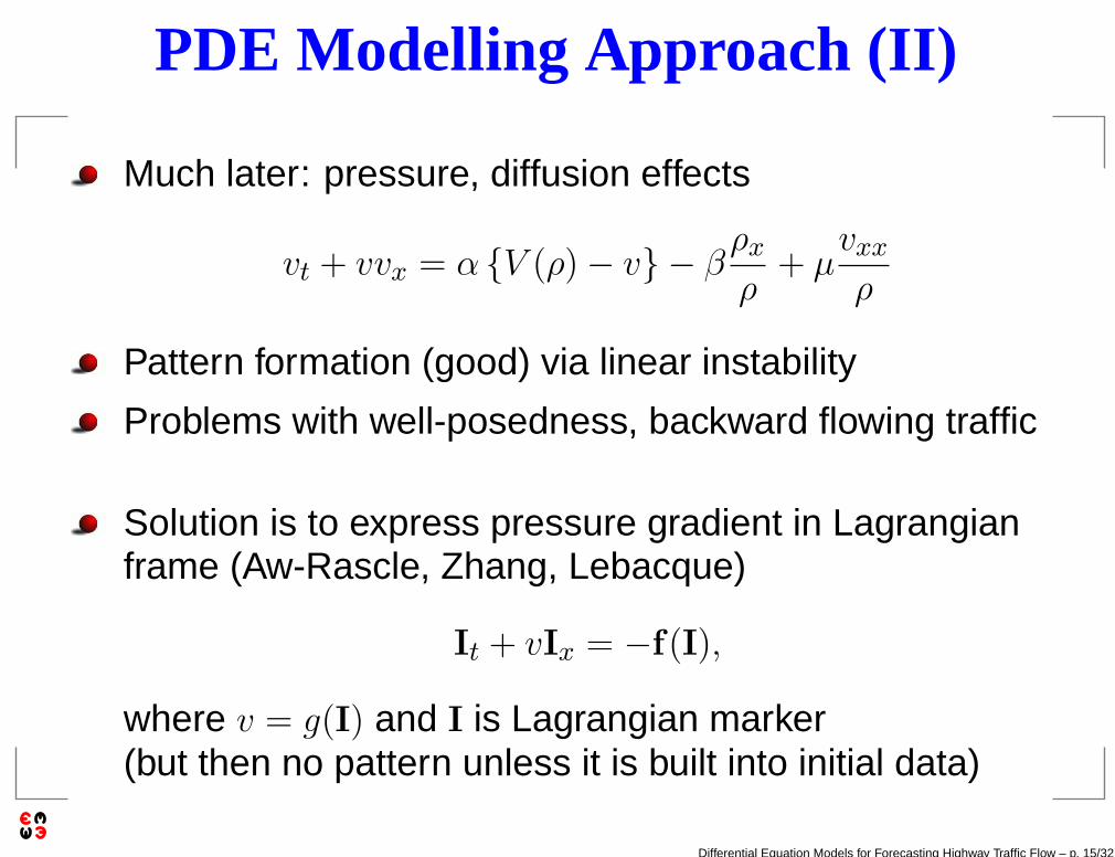
Much later: pressure, diffusion effects

vt + vvx = α {V (ρ) − v} − βρx

ρ+ µ

vxx

ρ

Pattern formation (good) via linear instability

Problems with well-posedness, backward flowing traffic

Solution is to express pressure gradient in Lagrangianframe (Aw-Rascle, Zhang, Lebacque)

It + vIx = −f(I),

where v = g(I) and I is Lagrangian marker(but then no pattern unless it is built into initial data)

Differential Equation Models for Forecasting Highway Traffic Flow – p. 15/32

Car following models

�����

�����

������

������

������

������

������������ ��������

����������

������������

������������

��������

��������

��������

��������

x

xnxn+1 xn−1

vn vn−1vn+1

hn

Typical form

xn = vn,

vn = f(hn, hn, vn) and generalisations

E.g. Bando model (1995) or extensions

f = α {V (hn) − vn} + βhn, α, β > 0

V is Optimal Velocity or Speed-Headway function

Differential Equation Models for Forecasting Highway Traffic Flow – p. 16/32

Equilibrium curves

0 0.5 1 1.5 2 2.50

0.1

0.2

0.3

0.4

0.5

0.6

0.7

0 1 2 3 4 50

0.2

0.4

0.6

0.8

1

1.2

1.4

1.6

1.8

2

0 0.5 1 1.5 2 2.50

0.2

0.4

0.6

0.8

1

1.2

1.4

1.6

1.8

2

speed

headway

speed

density

density

flow

no observationsdue to sensing method

Differential Equation Models for Forecasting Highway Traffic Flow – p. 17/32

Empirical equilibrium curves (again)

0 10 20 30 40 50 60 70 800

20

40

60

80

100

120

140

160

0 10 20 30 40 50 60 70 80 900

5

10

15

20

25

30

35

40

45velocity (km/h)

density (veh/km) density (veh/km)

flow

(ve

hs/m

in)

lane 2 measurementsonly

oscillations

free

flow

congestioncongestion

freeflow

Validates state relationship v = V (ρ), flow = ρV (ρ)v is velocity, ρ is density

Note high flow variation in congested conditionsIs our explanation correct?(two-phase vs three-phase arguments)

Differential Equation Models for Forecasting Highway Traffic Flow – p. 18/32

Outline of talk

Data part I (fairly standard)

Differential equation models

Data part II (revolutionary)

Differential Equation Models for Forecasting Highway Traffic Flow – p. 19/32

Three Key Ideas

Intelligent Transport Systems infrastructure is routinelycollecting data which we should exploit to rationaliseand improve traffic models

Lots of dumb data (cheap) plus clever analysis may beas good as a little clever data (expensive)

I want to advertise a new data set which I am makingavailable to the community

http://www.enm.bris.ac.uk/trafficdata

Differential Equation Models for Forecasting Highway Traffic Flow – p. 20/32

NGSIM project / helicopter photography

Expensive data!!!!

Differential Equation Models for Forecasting Highway Traffic Flow – p. 21/32

Individual Vehicle Data: pair of loops

1 2 3lanes

1 2 3lanes

time,

6 s

ecs

12589

108

96

117

113

89

129

95

119

111

113

location A location B Individual vehicledata gives‘helicopter view’(speeds km/h)

Location B is 100mdownstream oflocation A: notelane change

Further spatialextent?

Differential Equation Models for Forecasting Highway Traffic Flow – p. 22/32

Ongoing trial

Piggy-backs on government trial of IDRIS hardware system— removes need for engineer’s terminals

Started January 2008

16 sites at 100m spacing near J4 on M42 including amerge (one carriageway only)

Exercise is ongoing (with some breaks)

Data is generally much cleaner than other IVD

Differential Equation Models for Forecasting Highway Traffic Flow – p. 23/32

Aerial View

http://www.enm.bris.ac.uk/trafficdata

Differential Equation Models for Forecasting Highway Traffic Flow – p. 24/32

6 sites× 20s of Individual Vehicle Data

1 2 3

5.4

5.4002

5.4004

5.4006

5.4008

5.401

5.4012

5.4014

5.4016

5.4018

5.402

x 104

85

103 117104

87

8998

107

107

10791

105

1 2 3

98

86

117101

107

88

89101

108

107

108

91111

1 2 3

104

89

119

100

107

88

10793

108

109

111

11487

117

1 2 3

104

88 119

108

101

89108

93

109

109

109

111

116

901 2 3

107

11988

113

99

10988

94

107

111

114

109

1 2 3

93

105

119

90 113

104

111

8789

101 117

109

113

time

(s)

Differential Equation Models for Forecasting Highway Traffic Flow – p. 25/32

Patterns in instrumented section (1)di

stan

ce (

km)

speed (km/h)

time (hrs)Differential Equation Models for Forecasting Highway Traffic Flow – p. 26/32

Patterns in instrumented section (2)

time (hrs)

speed (km/h)

dist

ance

(km

)

Differential Equation Models for Forecasting Highway Traffic Flow – p. 27/32

Outline of re-identification algorithm (1)

NB no rocket science

First step: partition data

Given an upstream record u find downstream records dfor which

|tu + ∆x/vu − td| < ǫ

Given a downstream record d find upstream records ufor which

|td − ∆x/vd − tu| < ǫ

Defines bipartite graph — partition it into maximalconnected components

Unique possible matches: components of size 1 × 1Can be used to learn length error statistics etc.

Differential Equation Models for Forecasting Highway Traffic Flow – p. 28/32

Outline of re-identification algorithm (2)Simple case: n × n bipartite component where n is smalli.e. n upstream records U and n downstream records DSeek ‘optimal’ bijection Π : U → D

For example, seek Π for

min∑

πijcij

cij measures length discrepancy, time discrepancy. . . (messy)(Hungarian / auction algorithms)

In practice: scores must take into account lane orderpermutations and are non-additive

All this messy: neural nets etc.

Greater than 99% accuracy in Phase 1

Differential Equation Models for Forecasting Highway Traffic Flow – p. 29/32

Does it really work?

0 5 10 15 200

5

10

15

20

25

30

35

40

45

50

TRIVIAL TRIVIAL TRIVIAL

time (hrs)

spee

d (m

/s)

OK

OK

OK

OK

ON

GO

ING

ON

GO

ING

Differential Equation Models for Forecasting Highway Traffic Flow – p. 30/32

Some Ideas for Projects (an invitation)

Camera trajectory data vs IVD — can they complementeach other (in fitting car-following models)?

Lane changing / lane-effect models calibrated in detail

Complex behavioural models (with respect to theweather, the variable speed limit, . . .)

Macroscopic theory revisited (experiment with filterwidth and test continuum assumption)

Generalisations / refinements of potential models whichuse the extra spatial information

Vehicle re-identification algorithms themselves(real-time operation?)

Differential Equation Models for Forecasting Highway Traffic Flow – p. 31/32

Thanks for Listening

http://www.enm.bris.ac.uk/trafficdata

Differential Equation Models for Forecasting Highway Traffic Flow – p. 32/32