DIFFERENTIAL EFFECTS OF SWEDISH ACTIVE

LABOUR MARKET PROGRAMMES FOR UNEMPLOYED ADULTS DURING THE 1990S

Barbara Sianesi

THE INSTITUTE FOR FISCAL STUDIES

WP01/25

Differential Effects of Active Labour Market Programs for the Unemployed

Barbara Sianesi *

Revised: August 2005

(First draft: October 2001)

Abstract: The differential performance of six Swedish active labour market programs for the unemployed is investigated in terms of short- and long-term employment probability and un-employment-benefit dependency. Both relative to one another and compared to more intense job search, the central finding is that the more similar to a regular job, the more effective a program is for its participants. Employment subsidies perform best by far, followed by trainee replacement and, by a long stretch, labour market training. Relief work and two types of work practice schemes appear by contrast to be mainly used to re-qualify for unemployment bene-fits. Keywords: Active labour market programs, evaluation, multiple treatments, propensity score matching, treatment effects. JEL classification: C14, J38, J65, J68.

Acknowledgements: I am indebted to my supervisor, Costas Meghir, for helpful comments and continuous guidance. I thank Anders Harkman and Per Johansson for invaluable informa-tion and detailed comments, and Jaap Abbring, Erich Battistin, Richard Blundell, Massimili-ano Bratti, Kenneth Carling, Anders Forslund, John Ham, Hide Ichimura, Andrea Ichino, Francis Kramarz, Edwin Leuven, Katarina Richardson, Jeff Smith, Paolo Sestito and partici-pants at the IVA conference, the Second Villa Mondragone Workshop in Economic Theory and Econometrics in Frascati (Rome), the Network of Excellence conference on “The Evalua-tion of Labour Market Policies” in Amsterdam, the Econometric Society Winter European Meeting in Budapest, the UCL Applied Micro seminar, the ESEM 2003 in Stockholm, the II Workshop ‘Brucchi Luchino’ in Milan, the Nordic Conference 2004 in Denmark and HM Treasury for discussions and suggestions. Thanks also to Kerstin Johansson for the municipal-ity-level data and to Helge Bennmark and Altin Vejsiu and again Anders Harkman for helpful institutional information and data issues clarifications. A very special thank to Susanne Ackum for encouraging this research and organising financial support through the IFAU. Fi-nancial support from the ESRC Centre for the Microeconomic Analysis of Fiscal Policy at the IFS is also gratefully acknowledged. * Institute for Fiscal Studies 7 Ridgmount Street London WC1E 7AE United Kingdom Tel: +44 (0)20 7291 4831 Fax: +44 (0)20 7323 4780 Email: barbara_s@ifs.org.uk

1

1. Introduction

Labour market interventions have been an important element of public policy in the US, Europe and

several other OECD countries for over two decades. In 1997, EU states even committed themselves

to ensure that every young unemployed is offered training, retraining, work practice, a job or other

employability measure before reaching 6 months of unemployment, the same applying to unem-

ployed adults before they reach 12 months.1 The OECD has also explicitly called for an expanded

use of such measures, together with a ‘reinforcement of their effectiveness’.2 In fact, confronted

with high and persistent unemployment3, several OECD countries have been introducing or expand-

ing their active labour market policy in the 1980s and especially 1990s.

But this surge in interest in active labour market programs (ALMPs) and concomitant rise in

public spending begs the obvious question of whether these numerous measures do indeed work

and whether they all work equally well. In fact, although programs such as job broking, re-training,

job creation in the public sector and subsidised employment are each aimed at improving the labour

market opportunities of the unemployed, their effectiveness may strongly differ.

Despite lower public outlays, the US have traditionally been at the forefront in the evaluation of

ALMPs. The focus of this literature has typically been on whether individual programs work (see

Friedland et al., 1997, and Heckman et al., 1999, ch.10, for extensive surveys). Since these pro-

grams generally offer a combination of active measures, the extent to which the uncovered effects

arise from skills-building activities as opposed to the other lower-cost activities that are bundled

with them remains largely unclear.4 Furthermore, even though different programs have been looked

at, they have not been compared against one another, but rather to the ‘no-program’ state (or to a

state of unspecified alternatives). An unequal performance of different programs compared to ‘no-

program’ may however also arise from the different type of individuals participating in the various

measures. Hence these comparisons do not allow one to properly assess whether the programs are

well targeted – in the sense that those who participate in program A perform better than if they had

gone on program B –, or whether there are programs that are uniformly better than others.

1 EU Council Resolution No.13200/97. 2 The OECD Job Strategy was launched in 1994. See OECD (1994), as well as (1996). 3 Although the US does not face as high an unemployment rate as the average OECD or European country, in some areas and for some subgroups, notably the low-skilled and ethnic minorities, the figures are rather comparable (e.g. in 2003, an average 8% rate for the OECD and 8.8% for OECD-Europe, though higher than the overall 6% in the US, are on the lower side of the over 10% rate for the low-skilled and blacks in the US). 4 See the discussion in Friedlander et al. (1997). Some progress has been made in determining the differential effects of a couple of service combinations in the JTPA and JOBS evaluations.

2

This paper exploits the potentially highly instructive institutional set-up in Sweden to directly as-

sess the relative performance of different programs.5 Building on a long-standing experience of

ALMPs (dating back to the 1930s), Sweden has been extensively relying on a rich menu of such

measures. This case is thus of special interest, since the same target population is exposed to the

same wide set of well-established programs whilst facing the same macro conditions and institu-

tional framework.6 A clear outlier in terms of ALMPs expenditure7, Sweden has also traditionally

enjoyed low unemployment rates by European standards, and was thus often regarded as a model

(see e.g. Layard et al., 1991). Indeed, the broad types of Swedish programs we consider closely re-

semble those available in other developed countries in terms of design and services offered (e.g. the

Swiss and German ALMPs, or the multiple options offered by the New Deal in the UK).

The available longitudinal data record the labour market history (to the day) of all unemployed

registered at public employment offices since 1991. These representative and very detailed adminis-

trative data allow one to capture both short- and long-term program effects, as well as how the ef-

fects of the various programs may differentially evolve over time. In the literature effects are by

contrast often evaluated at a given – and arbitrary – point in time, such as on the last observation

day, or after a year. This misses out on the dynamics: the effect of a given program may differ in

the short- from the long term, and different programs may take different lengths of time to produce

an impact on labour market outcomes. Long enough follow-ups are needed to assess how sustained

the returns to participation in different programs are.

Finally, broad lessons can be learnt from the Swedish case as to the interdependence between

passive and active measures, the subject of recent policy debate.8 Passive unemployment benefits

support individuals whilst unemployed, but also affect work incentives. If – as in Sweden until 2001

5 Microeconometric studies looking at the relative effects of different programs include Frölich et al. (2004), Larsson (2003) and Carling and Richardson (2004) for Sweden, and e.g. Gerfin and Lechner (2002) and Gerfin et al. (2004) for Switzerland; Brodaty et al. (2001) and Bonnal et al. (1997) for France, and the earlier work by Ridder (1986) for the Netherlands. 6 The evaluation of universal and long-established programs does not incur in a number of potential biases. First, scale bias would arise if the scaling up of pilots to universal participation changes community norms or combines with pat-terns of social interaction or information diffusion which might affect program impacts (Garfinkel et al., 1992). Entry effects relate to the possibility that once a tested program is made permanent and extended to the entire eligible popula-tion, the entry or exit of individuals from the criteria that define eligibility might be affected (Moffitt, 1992). Finally, as offices learn about the administration and delivery of a new program, the actual ‘treatment’ might differ from the one that was evaluated. 7 While the average OECD country spent between 0.7 and 0.9% of its GDP on ALMPs during the 1980s and 1990s, the figure for Sweden remained well above 1%, peaking to over 3% in the severe recession of the 1990s. The programs also involve a very large proportion of the Swedish labour force; in 1997 for instance, the equivalent of 4.5% of the labour force participated on average in such measures (excluding those for the disabled). 8 Cf. guideline II of the 1998 Employment Guidelines (EC, 1998) and the ensuing national employment plans.

3

– participation in an ALMP renews entitlement to unemployment compensation, not only are incen-

tives to search and accept job offers likely to be reduced, but this benefit-renewing feature of the

programs may seriously undermine their own effectiveness.

This paper evaluates the six programs that were available to entitled unemployed adults in 1994:

labour market training, two work experience programs (workplace introduction and work experi-

ence placement), public relief work, trainee replacement and job subsidies.9 Their differential per-

formance is investigated both relative to one another and vis-à-vis more intense job search in open

unemployment. For participants in a given program we thus estimate the effect of joining that pro-

gram compared to joining an alternative program, as well as compared to waiting longer in open

unemployment.10 Effects are evaluated month by month for 5 years since program entry.

Helping the unemployed back into work is a primary aim of ALMPs, and the stated one in Swe-

den. We thus focus on employment rates over time, summarising program effects on both job find-

ing probability and job attachment while employed. This allows us to investigate if and how the

various programs differentially endow participants with skills and working habits that enhance their

employment prospects in the short- and long-run. Special attention is also devoted to differential

program impacts on individual benefit collection probability over time, allowing us to directly cap-

ture the influence that benefit renewability may have on the effects of the various programs.

The next section outlines the Swedish labour market policy and the six programs being evalu-

ated. Section 3 describes data and sample choice. Section 4 clarifies the evaluation questions to be

addressed and sketches the evaluation approach in the multiple-treatment framework. Our data in-

clude a wide array of demographic, human capital and labour market variables, as well as the case-

worker’s time-varying subjective appraisal of various factors relating to the overall situation, char-

acter and needs of service of the job-seeker. Such informational richness has motivated the match-

ing approach taken in the paper. Section 4 devotes considerable attention to the discussion of the

plausibility of the underlying identifying assumption. The set of empirical findings is presented in

Section 5, before concluding in Section 6 with a summary and overall appraisal of the results.

9 Sianesi (2001) offers a purely non-technical overview of issues for the evaluation of the Swedish active labour market policy as well as an appraisal of related empirical results, including some selected results from this paper drawn to-gether with other findings from Sianesi (2004) and from additional analyses. 10 The latter choice of comparison state is driven by an institutional set-up where individuals will sooner or later join a program provided they are still unemployed (see Section 4.1). In such a context, Sianesi (2004) has proposed looking at the impact of joining a program at a given time in unemployment compared to not joining any program at least up to then. While Sianesi (2004) has combined all the programs into one treatment in order to look at the performance of the Swedish system in its entirety, the present paper adapts this strategy to a multiple treatment framework. Disaggregating

4

Our findings highlight some interesting conclusions. The magnitude and even the sign of the

various treatment effects were found to change over time since program entry, which underscores

the importance of being able to look at outcomes in both the short- and longer term. Overall, pro-

gram effects were found to be widely heterogeneous across program type, with different types of

measures often displaying diametrically different impacts on individual outcomes. In particular,

those programs providing subsidised job experience and on-the-job training (i.e. job subsidies and

trainee replacement) were found not only to be cheaper, but considerably more effective than voca-

tional classroom training in terms of participants’ labour market performance. Further, the more

closely the task performed on a program resembles regular work, the higher are the benefits of the

program to its participants. In fact, those programs on which participants did not perform particu-

larly relevant tasks (i.e. relief work, workplace introduction and work experience placement) ap-

peared to be simply used as vehicles to renew benefit eligibility, inducing job-seekers to drift into

long-term unemployment and benefit dependency.

2. The Swedish labour market policy

The Swedish labour market policy has two main and interlinked components: a variety of active

labour market programs and an unemployment benefit system.

The stated overall purpose of the Swedish labour market programs is to prevent long periods out

of regular employment and to integrate unemployed and disadvantaged individuals into the labour

force. There are various kinds of programs, some specifically targeted at particular groups (e.g. the

young or the disabled) and the rest open to anyone registered at an employment office.

This evaluation focuses on the six main programs open to adult unemployed workers in the mid

‘90s: labour market training, workplace introduction (API), work experience placement (ALU), re-

lief work, trainee replacement and employment subsidies.11 With the possible exception of trainee

replacement12, these programs typify those commonly available in other OECD countries. Table 2.1

contrasts their main features, and places them within the OECD classification of ALMPs.

To gain access to any program, one needs to be registered at a local official employment office.

the program treatment into its main components allows us not only to evaluate one program against another, but also to assess how heterogeneous the impacts of the different programs are compared to open unemployment. 11 Two programs are excluded from the analysis on the basis that they are targeted to (or attract) quite specific sub-groups of the unemployed: self-employment grants (for those wishing to establish their own new business, with both a business idea and a financial plan approved by the offices) and vocational rehabilitation (for those with occupational disabilities needing specialised resources for in-depth counselling and job-preparation measures). 12 Job rotation programs of this type are available e.g. in Austria, Finland, Norway and Portugal.

Table 2.1 Synoptic table of the main features of the programs

Program Aim Eligible Employer Training Task Compensation a Cost b OECD c Classification (% spending)

EMPLOYMENT SERVICES

fill job openings quickly; job search assistance and training

job seeker activities

UI/KAS if entitled

Public employment services &

administration (17%)

LABOUR MARKET TRAINING (AMU)

equip individuals with skills to find jobs more easily

>20 private & public providers

vocational classroom training

TA/BA; course free

1,992 Labour market training (23%)

WORK PRACTICE

Work experience placement (ALU)

prevent exhaustion of benefits whilemaintaining contact with working life and enhancing working habits

entitled ≥20

90% public & non-profit

otherwise not performed

TA/BA 1,328

Workplace introduction (API)

maintain contact with working life; obtain workplace training, job-experience and references

≥20 private & public practical vocational

training

otherwise not performed

TA/BA 999

TEMPORARY JOB

Relief work specially created temporary jobs to maintain working skills and habits, also to avoid benefit exhaustion

>25 2/3 in public sector (municipalities &

state organizations)

otherwise not performed

according to collective agreement

1,315

Subsidised

employment: Direct job creation

in public & nonprofit sectors (15%)

Trainee replacement

enhance skills of employee while providing an unemployed individual with work experience

≥20 80% public sector on-the-job practice

regular according to collective agreement

1,095 –

EMPLOYMENT SUBSIDIES

increase chance of job offers; establish permanent employment relation

≥6m unemplm.

≥20

private sector only; from ‘97 some

industries excluded

on-the-job practice

regular

according to collective agreement

853 Subsidies to private-sector empl. (& start-up grants)

(15%)

Notes: Information has been gleaned from various sources, in particular, Swedish Institute (1997). a TA is training allowance equivalent to the UI or KAS the individual would have been entitled to; BA is the basic amount (SEK103 per day; in 2004 USD less than 15) if the individual is not entitled. b Total monthly cost per participant in 1998 expressed in 2004 USD (AMS, 1998, reported in Carling and Richardson, 2004, Table 1). cCategory within the OECD classification of ALMPs and respective % out of total spending on ALMPs by the average OECD country in 2000 (OECD database on Labour Market Programs). The remaining two categories are measures for youth (13%) and for the disabled (17%).

5

The six programs under consideration are additionally open to adults only (over 20 or 25), while

ALU requires the individual to be entitled to unemployment compensation, and job subsidies are

targeted at the long-term unemployed. The latter may often be regarded as a mere guideline,

though, since 20% of the job subsidy participants in our data have spent less than the required 6

months in open unemployment prior to joining. Our sample satisfies the eligibility rules in terms of

registration, age and entitlement, while we shall control very carefully for unemployment duration.

Whilst on a program, participants either earn the stipulated wage and other benefits on their

‘temporary’ workplace, or the equivalent of the unemployment benefit they would have drawn as

openly unemployed. Most programs have a maximum duration of six months (under special cir-

cumstances renewable for another six), though participants stay an average of 4-5 months.

Labour market training, by far the most expensive measure, is intended to augment participants’

human capital via full-time, formal teaching of new vocational13 skills.

A second type of program offers workplace traineeship to maintain and enhance contact with

working life and gain practical experience, good working habits and references from which to later

benefit on the regular labour market. Work experience placement (ALU) was introduced at the

deepening of the recession in 1993 with the explicit aim to prevent entitled individuals from ex-

hausting their benefits. In fact, individuals need to be eligible to either UB or KAS to participate in

this scheme, which can involve almost any kind of activity (the most frequent tasks being in ad-

ministration and construction). Workplace introduction (API), which replaced a number of older

job-experience programs, offers unemployed individuals a period of workplace training.

A third kind of measure provides unemployed workers with a temporary job. Relief work in-

volves specially created temporary jobs, mostly in the public sector. The oldest measure for creating

employment, it has diminished in importance during the 1990s, becoming primarily used for indi-

viduals at risk of losing their unemployment benefits (Swedish Institute, 1997). In particular, indi-

viduals who run out of compensation are in principle granted the right to a relief job. In a trainee

replacement scheme, an unemployed individual replaces a regularly employed worker who is on

leave for education. This measure thus allows an unemployed worker to acquire valuable work ex-

perience, while creating an opportunity for firms to update the skills of their employees.

Finally, employment subsidises offer a temporarily subsidised job opportunity to acquire job-

13 To reduce the heterogeneity in courses offered, we only consider vocational training. Non-vocational courses are by contrast aimed at helping workers with basic educational insufficiencies to move on to further education or to other pro-grams, rather than directly into a job.

6

specific human capital.

While all the programs aim at improving participants’ employment prospects, they differ in the

kind of skills they provide and in the way they provide them. At the one end of the spectrum, labour

market training provides vocational classroom training of new skills deemed in demand. API has a

strong emphasis on practical vocational training; similarly, ALU and relief work may provide par-

ticipants with job experience and improve their working habits. Participants in these three programs

are however prevented – at least formally – from performing tasks that a regularly employed indi-

vidual would otherwise do. Although it is likely for such a rule to be often interpreted more as a

recommendation than as a strict guideline14, to the extent it is adhered to, the type of on-the-job

practice acquired may not be expected to be particularly marketable.

Like the two work practice schemes and relief work, trainee replacement and employment subsi-

dies offer the opportunity to invest in job-specific human capital; in these cases, though, the partici-

pant does in fact replace ordinary labour. Finally, while trainee replacement – a deputyship for the

employee on study leave – is intrinsically a temporary opportunity to gain job-specific experience,

employment subsidies implicitly seek to influence an employer’s hiring decisions towards retaining

the worker after completion of the program.

A final consideration relates to the first row in Table 2.1. Individuals searching for a job as

openly unemployed can benefit not just from standard job information and matching of vacancies to

applicants, but also from the ‘job-seeker activities’, which include search-skill-enhancing activities

(e.g. training courses on how to apply for a job) and motivation-raising activities. In Sweden, the

‘no-treatment’ status to which program participation has to be compared to is thus not a complete

absence of intervention, but these baseline services offered by the employment offices. In some

countries this kind of assistance is in fact considered a program in its own right.15

As to unemployment compensation, benefits are provided in two forms16, the most important one

being unemployment insurance (UI). UI benefits are quite generous by international standards

(daily compensation being 80% of the previous wage17) and are available for a total of 60 weeks,

more than twice the maximum duration in the US. To be eligible to UI an unemployed person regis-

tered at an employment office and actively searching for a job must have been working for at least 5

14 Circumstantial evidence in Hallström (1994; from Ackum Agell, 1995) shows that sponsors, participants and case-workers believe that these projects do often replace jobs that are part of the organisers’ normal activity. 15 An example is the Gateway period of the UK New Deal program for the unemployed. 16 Those not entitled to any unemployment benefits may receive means-tested social insurance. 17 This maximum level has changed a few times during the 90s. The system also has a ceiling.

7

months during the 12 months preceding the current unemployment spell.18 Once receiving UI, an

offer of ‘suitable’ work – or of a labour market program – must be accepted; refusal to accept a

job/program might lead to expulsion from compensation (the ‘work test’).

The second form of unemployment compensation is KAS. This supplementary system, mainly

designed for new entrants in the labour market who usually are not members of any UI fund, is

roughly half as generous as UI, both in terms of amount and duration of benefits. Claimants are sub-

ject to a work condition similar to the one for UI, which can however be replaced by the education

condition of having finished at least one year of school in excess of the 9 compulsory ones.

The passive and active components of the Swedish labour market policy used to be closely

linked: before 2001, 5 months spent on a program (or completion of a training course) would qual-

ify for a renewed spell of unemployment compensation. Even though the maximum benefit period

was nominally fixed, it thus used to be possible to extend it indefinitely by using program participa-

tion to renew eligibility. Programs could thus actually end up reinforcing the work disincentives

associated with the benefit system, this being especially the case for individuals entitled to benefits.

3. Data and sample selection

Our dataset is constructed from two main sources, reflecting the program component (Händel) and

the benefit component (Akstat) of the labour market policy. Händel is the unemployment register

and contains information on all unemployed individuals registered at the public employment of-

fices. Available from 1991, this longitudinal event history dataset provides each individual’s labour

market status information over time, together with important characteristics of the job-seeker and of

the occupation sought. The information regarding the reason for ending the registration spell (e.g.

obtained employment, gone on regular education or left the workforce) has been used to impute the

individual’s labour market status in between registration periods. Akstat, available from 1994,

originates from the unemployment insurance funds and records information – in particular on un-

employment benefit receipt, previous wage and working hours – for individuals entitled to benefits.

As to sample choice, individuals need to be homogeneous in those basic characteristics which

determine eligibility to all the programs under examination. Only then will it be relevant to examine

their outcomes had they chosen a competing program. We focus on adults (aged over 25) who are

entitled to unemployment benefits. In addition to their exclusive access to one of the programs

18 There is also a membership condition, requiring payment of the (almost negligible) membership fees to the UI fund for at least 12 months prior to the claim.

8

(ALU), entitled jobseekers are of special policy interest, since they are the group whose participa-

tion incentives are most likely to be affected and for whom the trade-off between productivity-

enhancing effects of the programs and the reinforced work disincentive associated with the benefit

system should be at its sharpest. An added advantage compared to non-entitled individuals is in

terms of data quality and availability: since registration at an employment office is a pre-requisite

for drawing benefits, our chosen sub-sample is a particularly representative one of the sub-

population of interest. The information for benefit recipients is thus especially reliable, but also

much richer, since it includes the Akstat data.

We look at the inflow into unemployment in 1994, the year when the unprecedented recession

that had hit the Swedish economy in the early 90s was at its most severe.19 Mainly dictated by the

need to exploit the information in Akstat, the choice of this year yields a sample of above-average

quality unemployed compared to the inflow in an average year. On the other hand, it is particularly

interesting to assess how successful the massive use of ALMPs during the recession was in bringing

their pool of participants back into work. It is exactly in periods of high unemployment when effec-

tive programs would be most needed.

We further restrict our sample to adult individuals who became unemployed for their first time20

in that year and were entitled to either UI or KAS. Additionally, individuals whose first program

was start-up grants, vocational rehabilitation or non-vocational training are dropped from the analy-

sis (see footnotes 11 and 13). These criteria lead to a sample of 30,800 individuals, followed from

the moment they register in 1994 to the end of November 1999.

Descriptive statistics of the various treatment groups are presented in Appendix B. Visual in-

spection of average characteristics clearly shows that participants in the different programs are in

fact quite distinctive groups. There seem to be several demographic, human capital and labour mar-

ket variables which systematically differ between the groups and which are most likely to affect

subsequent labour market performance.

19 From less than 3% in 1989 and 1990, unemployment jumped to 9% in 1992, reached its peak of 13.5% in 1994 and then stayed around 13% until 1997. 20 Since Händel starts in August 1991, strictly speaking we can only ensure that individuals registering in 1994 have not been unemployed at any time during the previous three years. Given however that it was exactly between these three years that Sweden experienced unprecedentedly high unemployment, the requirement is likely to be quite binding, mak-ing us reasonably confident that most of our individuals are indeed first-time unemployed.

9

4. The evaluation problem in the Swedish institutional set-up 4.1 Evaluation questions and evaluation approach The Swedish institutional set-up poses a few interesting methodological issues which have to be

resolved before deciding on the evaluation strategy. In particular one needs to be very explicit about

the definition of the relevant treatments. While Section 2 has already described the six programs of

interest, these take place continuously over time and are open to all registered job-seekers; unem-

ployed individuals are in fact often observed to participate in different programs at different times

during their unemployment history. As our sample is one of first-time unemployed, we focus on the

first program individuals may receive within their first unemployment experience.21 Furthermore,

since the observed program duration is endogenous22, we start measuring the causal effect at entry

into the program and view any lock-in effect whilst on the program as a constituent part of the ef-

fect. The treatments are thus in terms of joining a given program right after having become unem-

ployed (thus not in terms of completing a given program, nor of taking only a given program).

When evaluating the effect of a program on some outcome, an essential part of the research

question concerns the comparison state. In addition to the effect of joining a given program com-

pared to joining a different one, interest often lies in assessing the effect of joining a given program

relative to no program participation at all. In the standard US program evaluation specification, the

program is administered at a fixed point in time, and individuals are either treated or non treated. In

Sweden, by contrast, not only are the programs ongoing, but any job-seeker can potentially join one

and will eventually join one at some time, provided he remains unemployed long enough. Indeed

one could argue that the reason an unemployed individual has not been observed to go on a program

is because he has found a job before enrolling. In the Swedish institutional set-up the definition of

non-participants cannot thus be the standard one, namely those individuals who are observed not to

enter any program. Since such individuals would de facto be observed to leave the unemployment

register, this approach would amount to selecting a comparison group based on future (and success-

ful) outcomes.23 Although a non-standard one, this evaluation problem is quite commonly encoun-

tered, in particular in the evaluation of ongoing programs which individuals sooner or later will join

21 The sequence of programs an individual goes through is not exogenously determined at the start of the unemployment spell. In our framework, any subsequent program participation is viewed as an outcome of that first treatment. Although subsequent take-up of other programs can thus be assessed in its own right (as done by Sianesi, 2004), to conserve space here we look at employment and compensated unemployment as direct measures of labour market performance. 22 Some programs require participants to continue job searching. The offices too continue to search; participants are in fact required to drop out of a program if a ‘suitable’ job is found for them.

10

provided they are still eligible (e.g. still unemployed).

The program participation process in Sweden is such that once an individual has become unem-

ployed, he and his case-worker are most likely to take their decisions sequentially over time in un-

employment. In particular, at any given moment the relevant decision is not whether to participate

in one of the programs or not to participate at all, but whether to join a program now or not to par-

ticipate for now, searching longer in open unemployment and knowing that one will always be able

to join later on. An evaluation question relevant for this set-up, proposed by Sianesi (2004), lets the

parameter of interest mirror this key choice open to the eligibles and evaluates the average effect,

for those observed to join a given program after a given number of months spent in open unem-

ployment, of joining that program when they did compared to further postponing the participation

decision by not joining any program at least up to then. Specifically, the comparison group com-

prises those individuals who are unemployed up until that time – and would thus be eligible to join

a program – but who do not join any at least as yet.

We thus investigate the differential effectiveness of seven different types of treatments: joining

labour market training, API, ALU, relief work, trainee replacement or job subsidies, as well as

searching longer in open unemployment.

In the following we briefly sketch the framework of Imbens (2000) and Lechner (2001), leaving

it to Appendix A to adapt it more formally to the institutional set-up just described.

Let D∈{0, 1, …, 6} denote actual assignment to a specific treatment – one of the 6 programs or

the ‘waiting’ option – and Yk the potential outcome an individual would experience were he to re-

ceive treatment k. We are interested in assessing the average effect for participants in program k of

participating in that program compared to receiving a different treatment k':

E(Yk–Yk' | D=k) = E(Yk | D=k) – E(Yk' | D=k) for k, k'∈{0, 1, …, 6}, k≠k' 24 (1)

While the first term of (1) is observed in the data, identifying assumptions25 need to be invoked

to estimate all the counterfactuals of the type E(Yk' | D=k), that is all the outcomes participants in k

would have experienced, on average, had they taken any treatment other than k. One such assump-

tion postulates that conditional on the value of observable characteristics X, the (counterfactual) dis-

23 Very recent work by Fredriksson and Johansson (2003) formalises this intuition. The discussion of an absent 'no-treatment' group was initiated by Carling and Larsson (2000a, b). 24 Note that in general this parameter is not symmetric: E(Yk–Yk’|D=k) ≠ –E(Yk’–Yk|D=k’) if participants in the two pro-grams systematically differ in characteristics related to the outcome. 25 Identification assumptions and estimation of treatment effects in non-experimental studies have been extensively looked at; for a comprehensive survey see Heckman et al. (1999).

11

tribution of Yk' for individuals joining program k is the same as the (observed) distribution of Yk' for

individuals receiving treatment k':26

D ⊥ (Yk, Yk') | X=x, D∈{k, k'} for k, k'∈{0, 1, …, K}, k>k' (2)

Methods like matching sample from (or reweigh) group k' to produce a matched group in which

the distribution of pre-treatment observables X is as similar as possible to the distribution in group

k. In order to adjust non-parametrically for observed differences in X between the two groups, how-

ever, all participants in k need to have a counterpart in group k' (common support requirement).27

Without imposing functional form assumptions or restricting impact heterogeneity across indi-

viduals, matching methods can eliminate the bias due to the difference in the supports of X in the

two groups being compared and the bias due to the difference between the two groups in the distri-

bution of X over its common support. Matching is however based on identifying assumption (2),

which assumes away the third potential source of bias identified by Heckman et al. (1998), selec-

tion on unobservables.28 Before turning to implementation and interpretational issues in section 4.3,

the next section thus discusses the plausibility of (2) in this application. To summarise some of the

main arguments, selection into the programs over time in unemployment is required to be unrelated

to labour market outcomes given a set of observables. In this analysis the relevant observables can

be chosen according to the findings of a Swedish survey directly asking job-seekers and casework-

ers about their decision criteria. The resulting set of controls is in turn particularly rich: employment

office and local conditions, detailed job-seeker’s characteristics and the caseworkers’ own subjec-

tive and time-evolving judgment of the client’s character, overall prospects and needs. Furthermore,

while the survey study identified the caseworker as the relevant decision-maker as to program

choice, from the received econometric evidence officers do not appear to be allocating their unem-

ployed clients to the different programs so as to maximize their subsequent employment prospects.

The next section thus makes a case for assumption (2) to represent a credible approximation and

hence for matching to be considered a feasible strategy in this informational and institutional setup.

26 Its weaker form in terms of conditional mean independence would suffice. 27 If there are regions where the support of X does not overlap for the two groups, matching has to be performed over the common support region and the estimated treatment effect redefined as the mean effect for those treated k falling within the common support. Alternatively, identification would rely on (parametrically) extrapolating from regions with positive probabilities for both the treatment states being compared to occur. 28 Note that a difference-in-differences approach is precluded here; outcomes are employment and benefit collection, and in the pre-program period all individuals are, by construction, unemployed collecting benefits.

12

4.2 Plausibility of the matching assumption Assumption (2) requires us to observe (and thus match on) all those differences between the various

treatment groups that are likely to affect their outcomes. We thus need detailed knowledge of the

factors that drive participation, as well as access to data suitable to capture those determinants of

participations that are also relevant to outcomes. In our application, not only do we have access to

detailed background information (including several direct indicators of individual heterogeneity),

but the choice of the relevant conditioning variables can benefit from the results of a Swedish sur-

vey directly asking job-seekers and placement officers about their participation decision criteria

(Harkman, 2000, as reported in Carling and Richardson, 2004). What we need to consider is

whether in deciding about participation these agents have access to and act upon information corre-

lated with labour market performance but that we cannot capture in our data. It is useful to sepa-

rately consider (A) the decision between waiting further in open unemployment or joining a (i.e.

any) program and (B) the decision to choose one specific program.

For decision (A) we need to control for all variables that, conditional on having reached a given

unemployment duration, influence both the decision to join a program as well as potential future

labour market performance were such decision to be postponed further. From Harkman (2000) it

appears that job-seekers largely base their decisions to participate in any program or not to partici-

pate on their subjective likelihood of employment. In so far as individual perceptions are accurate

enough, this subjective assessment will reflect actual potential employment outcomes. It is thus cru-

cial to identify enough information apt to capture these individual perceptions. We accordingly con-

trol for a whole set of variables intended to characterise the individual’s past employment history as

well as his current employment prospects, including his assessment thereof.

The only unemployment experience of individuals in our sample relates to the present unem-

ployment spell, a fact which is greatly informative of their labour market history. Entitlement status

further reflects a certain degree of labour market attachment due to the work requirement UI-

recipients have to fulfil.29 Previous working hours (a proxy of the extent of past labour market in-

volvement) and the pre-unemployment wage (conditional on qualifications, a summary statistic of

individual productivity) are additional important individual attributes which characterise the

worker’s overall earlier labour market situation; interestingly, such information is not necessarily

known by the caseworker. As to present employment prospects, we control for elapsed unemploy-

ment duration, benefit receipt status, demographics, several dimensions of human capital and a

13

number of direct indicators of individual heterogeneity.

Specifically, individual perceptions about one’s employment likelihood are likely to change over

time spent in unemployment. Elapsed unemployment duration should thus capture important unob-

servables in this dimension; more generally, in the presence of duration dependence and/or unob-

served heterogeneity, it is crucial to ensure that the comparison individuals have spent in unem-

ployment at least the time it took the treated to join. Elapsed unemployment duration is also an im-

portant X variable for directly explaining the joining decision, given some (albeit loose) regulations

(e.g. for job subsidies), as well as incentives related to unemployment benefits running out. As to

the latter, for a given elapsed unemployment duration we additionally control for benefits expiring

at that time or for benefits having run out by then.30 A binding ceiling in terms of compensation

amount finally controls for job-seekers facing a compensation rate effectively below 80%.

Demographic factors such as age, gender and citizenship, as well as the occupation being sought

are also important determinants of labour market prospects. Part-time unemployment spells denote

individuals who are still maintaining contact with the regular labour market and are probably both

subject to less human capital depreciation and in a better position to look for a (full-time) job, by

exploiting their bargaining position and additional contacts.

Human capital information is available in terms of specific education, general education and oc-

cupation-specific experience. The latter is a subjective indicator of the amount of experience for the

job being sought. It can be viewed as a summary statistics of the amount, effectiveness, transferabil-

ity and obsolescence of previous human capital accumulation, on-the-job training and learning-by-

doing, but also – together with the subjective indicator of education for the profession sought – as a

self-assessment by the unemployed individual of the strength of his own chances of re-employment.

Finally and most crucially, we exploit several direct indicators of individual heterogeneity likely

to be highly relevant in terms of employment prospects. Specifically, we have retrieved information

as to an overall evaluation by the officer of the situation, character and needs of service of the job-

seeker. This assessment relates to the job-seeker’s degree of job readiness (if judged to be able to

take a job immediately, to be in need of guidance or to be difficult to place), as well as to the job-

seeker’s preferences, inclinations and urgency to find a job (if willing to move to another locality, if

looking for a part-time job, if already having a part-time job). We also exploit a summary statistic

29 An indicator of KAS entitlement controls for the alternative way to fulfil the ‘work’ requirement. 30 Elapsed unemployment duration is only an imperfect predictor of benefit receipt, since job-seekers may decide to save their benefits for later, be suspended etc.

14

directly capturing selection into the programs (if the job-seeker has been offered a program and is

waiting for it to start). Note in particular that the caseworker may update and revise this subjective

judgement during his client’s unemployment spell. This time variation in the assessment of the

prospects and needs of the job-seeker is an additional key feature we can exploit to control for the

program joining decision over time in unemployment.

Another way to view condition (2) is that individuals are myopic conditional on observables:

given X, outcome-related information about the future plays no role in individual decisions to join a

program at u or to else wait longer. The discussion of individually perceived employment prospects

as the prime determinant of the program joining decision has thus to also consider the possibility of

anticipatory effects in terms of future employment. In particular, if some job-seekers know that

their former employer is going to call them back (e.g. they are seasonal workers, or have a credible

agreement with their employer allowing them to temporarily collect unemployment benefits), they

are likely to have fewer incentives to participate in the programs at any given month in unemploy-

ment; at the same time, they are observed to actually find employment. Additional observables in-

cluded to control for potential anticipatory effects of this kind include the occupation/skill type of

the job-seeker and the month of registration, which should help capture seasonal unemployment.

More generally, though, (2) would be violated if an individual waiting longer has decided to do so

because he has received a job offer and hence knows that he will be hired shortly. How serious this

issue is going to be in our case thus largely depends on the typical time span between job offer and

job commencement (and whether or not an individual who is going to start a job typically remains

or is allowed to remain registered at the employment office in the meantime). Note also that if the

time of job commencement is not too near, a caseworker’s decisions may provide additional ran-

domness in program participation patterns, since for entitled individuals the proposal of a program

can be used as a ‘work test’, whereby refusal to participate may entail suspension from benefits.

Our evaluation question concerns the effect of joining a given program at a given time compared

to later or never, thus requiring (2) to also hold in terms of future program participation, viewed as

an outcome. Controlling for elapsed time spent in unemployment is once again crucial, in that ap-

proaching benefit exhaustion would make an individual more likely to join a program or, if having

to wait longer, more likely to enter a program later on or to intensify job search (or lower one’s res-

ervation wage). As to anticipatory effects, (2) would be violated if an individual decided not to par-

15

ticipate at time u because he knows that he will join at some later date. This is not very likely.31

Additionally, as mentioned above, a very interesting piece of information in the data is an open un-

employment sub-spell where the job-seeker is waiting to enter a labour market program. Having

gone through the assignment process and having been offered a place makes it more likely for the

individual to join a program rather than waiting; had he not joined now, he would be more likely to

join later on or to decrease his job search in anticipation of joining. Like the caseworkers’ subjec-

tive judgements, this offer (or waiting-for-a-program) status changes over time in unemployment.

Turning now to decision (B), i.e. choosing one among the available programs, condition (2) re-

quires the evaluator to have access to all the variables that jointly influence such a choice and po-

tential future outcomes. Note first that all our individuals have access to the same choice set, the

only relevant recommendation being the one requiring a certain length of the unemployment period

prior to enrolment, for which we carefully control. Benefit renewability rules and individual com-

pensation while on the programs are similarly comparable across programs.

Harkman (2000) finds that individual self-selection into different programs is likely to be a mi-

nor issue in Sweden, in that unemployed workers tend to value the various programs equally. By

contrast the caseworkers do seem to have clear ideas about which type of program is suitable for

their clients, based on individual characteristics. Since the relevant decision-maker thus appears to

be the caseworker, the only issue we need to focus on is whether he acts upon information which is

unobserved to us yet correlated with clients’ potential outcomes.

We do however observe not only important characteristics of the job-seeker (e.g. educational

qualifications for possible cream-skimming for training programs), but also the caseworker’s own

subjective, synthetic and evolving evaluation of the overall situation and needs of service of his cli-

ent as described above. In a sense, the caseworker reveals, updates and records in the data a syn-

thetic appraisal of various factors, including some which may have been originally unobserved to

us. Our assumption then translates into the requirement that caseworkers act idiosyncratically given

worker characteristics and their own assessment of their client.

A final issue relevant for both decisions (A) and (B) relates to the local labour market conditions,

identified in the literature as a key variable to be controlled for (Heckman et al., 1997). In Sweden,

31 The institutional nature of the system (a continuous flow of different programs often on an individual, ad hoc basis) should make it less likely for a job-seeker to have to turn down a program offer perceived as second-best in order to wait for a free slot on his first-choice program (this would also reduce the likelihood of an ‘Ashenfelter dip’ problem in terms of reduced job search prior to participation). Even if he did wait, though, he would not enter his first-best program with certainty, but would still be exposed to the possibility of finding a job or deciding (or be forced) to join another

16

county labour boards have overall responsibility for labour market policy in each respective county,

and from the mid 90s municipalities have become increasingly involved in the decision-making as

to ALMPs. This shift towards decentralisation has given rise to new financial incentives (Lundin

and Skedinger, 2000). In particular, municipal budgets may be favourably affected by moving the

unemployed from social assistance (funded by the local authorities) to programs (financed by the

central government); some programs (e.g. relief work) may subsidise labour in the services typi-

cally provided by the local authorities; and programs may serve as a means of maintaining the local

municipal tax base by reducing geographical mobility among job-seekers. It is thus quite possible

that counties or municipalities facing different labour market conditions may favour a different bal-

ance between program and unemployment policies, as well as a different mix of programs.

In addition to county dummies, we have thus constructed the local ‘program rate’, given by the

number of participants in the six programs as a proportion of all individuals registered (as openly

unemployed or program participants) at the individual’s municipality. This time-varying indicator

provides information as to the local program capacity (e.g. in terms of slots available). Similarly, a

series of time-varying single ‘program ratios’ at the municipality level, given by the share of par-

ticipants in a given program over all participants in the six programs, is meant to reflect the pro-

gram mix at that municipality and time. Such indicators are intended as a parsimonious way32 to

capture unobserved local aspects which are likely to be relevant for program joining/choice decision

and individuals’ potential labour market performance.33

In sum, for individuals who have reached the same unemployment duration and who are similar

in terms of all the individual and local characteristics described, the decision to join a program at

that time rather than at least not yet, or the decision to join a given program rather than another need

to be random, i.e. to depend on factors unrelated to future potential outcomes. Sources of this re-

quired random variation conditional on our X’s can stem from job-seekers’ idiosyncratic prefer-

ences or random variation in their outlook on their employment prospects at a given time. On the

officer’s side, for given client characteristics, own judgement as to the client’s job readiness at a

given time and employment office incentives regarding participation at that time, this randomness

program in the meantime. 32 There are 289 municipalities and 484 employment offices in our data. 33 Local program capacity at a given time may affect the possibility for a job-seeker to join a program at that time as well as the officers’ scope for program selection, while offices facing more difficult local conditions may be more ac-tive in placing individuals on programs (e.g. to lighten the burden on the municipal budget or to decrease the number of openly unemployed in the municipality). Similarly, the program mix may affect program choice, while offices facing high unemployment may favour different programs (e.g. the cheapest, or those which subsidise the municipality).

17

can be based on caseworkers’ idiosyncratic preferences, incentives and experiences, as well as pro-

pensity (and strictness) to apply the work test.

One key point is that we can also exploit bottlenecks in the system, since we are able to condi-

tion on whether an individual has been offered and is waiting for a program, but cannot yet join,

due e.g. to start dates of a training course, a work-experience project or an employee taking leave

for a replacement scheme. A similar lack of appropriate conditions related to a program may also

provide randomness in the decision to join a program rather than another one.

Given this very rich set of observables, we thus require that selection into the programs is fully

driven by factors, such as the ones just described, unrelated to potential outcomes. In fact, case-

workers do not seem, in general, to be allocating their clients so as to maximize their subsequent

outcomes. For Sweden, Frölich (2001) has found that compared to the observed assignment to four

types of rehabilitation programs, an optimal allocation of participants would have yielded large

gains in the form of an over 20% higher re-employment rate.34

4.3 Implementation An important practical result by Rosenbaum and Rubin (1983) for the binary treatment case

D∈{0,1} is that the propensity score Pr(D=1|X), a scalar giving the probability of being treated

conditional on X, provides a parsimonious way to adjust for differences in the (generally large) full

set of characteristics X between treated and non-treated groups, formally: D⊥X | Pr(D=1|X). More

generally, a balancing score b(X) is a function of X, such that conditional on it, the characteristic X

are ‘balanced’ across the treatment groups, i.e. D ⊥ X | b(X).

Being here interested in the separate pair-wise comparisons of the various treatments, we need to

find a balancing score ensuring the balancing of the X’s in the two sub-populations of interest for

each separate comparison. For k and k' we need to find a b(X) such that

D ⊥ X | b(X), D∈{k, k'} (3) or equivalently such that35

E[Pr(D=k | X, D∈{k, k'}) | b(X)] = Pr(D=k | X, D∈{k, k'}) ≡ Pk|kk'(X) and 0< Pk|kk'(X) <1.

In our case of separate pair-wise comparisons of the various treatments, the conditioning variable

(balancing score) of minimal dimension which ensures the balancing of observables in the two sub-

34 Analogous conclusions are reached by Lechner and Smith (2003) for Switzerland (see also the similar evidence they review for other countries). 35 Cf. Theorem 2 by Rosenbaum and Rubin (1983) and proposition 1 in Lechner (2001). See also Brodaty et al. (2000).

18

populations of interest k and k' is thus still given by a scalar, the conditional choice probability of

treatment k given either treatment k or k':

| ' ( | )( )( | ) ( ' | )

k kk Pr D k XP XPr D k X Pr D k X

==

= + =

Under (2), the required counterfactual can then be estimated as

| '' ' | '( | ) [ ( | ', ( )) | ]k kk

k k k kkP

E Y D k E E Y D k P X D k= = = =

One way to apply such results is to control for systematic differences in observed characteristics

by matching participants in k to individuals receiving k' based on a balancing score b(X). For any

pair of treatments k and k', under assumption (2) the average outcome experienced by the matched

pool of k'-participants identifies the counterfactual outcome participants in k would have experi-

enced, on average, had they taken treatment k' instead.

Both the identification conditions and the balancing scores have been defined just taking account

of the two sub-samples participating in the two treatments which are the object of a given compari-

son, de facto ignoring the multi-program nature of the environment the individuals face. As Lechner

(2001) clearly points out, when interested in comparing two programs for participants in one of

those two, the existence of multiple treatments can in fact be ignored, since individuals who do not

take part in either program considered are not needed for identification.

However, estimation of the treatment probabilities does offer an opportunity to capture the mul-

tiplicity of options open to individuals. In the Swedish context we argued above that it is also im-

portant to model the month-by-month decision-making process of the individual/caseworker. A way

to accomplish this is to model the effect of unemployment duration (as well as of both fixed and

time-varying characteristics) on the various options open to an individual at any given point of time.

In particular, all our individuals start by registering as (first-time) unemployed. At any given month

U=u in their first unemployment spell, they can ‘decide’ between a set of M=11 exhaustive and mu-

tually exclusive options: to participate in one of the six available programs, to continue searching

for a job full-time as openly unemployed, to find (or decide to accept) a job, to go on regular educa-

tion, to leave the labour force through another channel, or to drop out of the unemployment register

for reasons unknown to the officials. By modelling the effect of unemployment duration on exit

type, one can thus simultaneously take account of the various exit routes from unemployment, of

right-censoring and of the effect of time-varying characteristics on individual choices.

As to the practical implementation, each individual unemployment spell is split into monthly

spells. Each of these new sub-spells is characterised by the duration month u the new sub-spell re-

19

fers to, by a corresponding treatment indicator and by those characteristics pertaining to, and events

taking place during that uth month of unemployment. The probability for an individual with charac-

teristics x of choosing option m after having spent u months in unemployment, Pr(D=m|U=u, X=x),

is then estimated36 and the corresponding balancing scores b(X) constructed.

Note that all we are interested in (ignoring potential efficiency considerations) is achieving (3).

Our interest in the estimation of b(X) as well as in the choice of matching method (which deter-

mines how the conditioning on b(X) is performed) purely lies in their combined ability to balance

the characteristics of the matched sub-groups being pair-wisely compared. The resulting quality of

the matched samples has thus guided the choice, for each pair-wise comparison, of the specification

for b(X) and of the matching estimator (cf. Appendix C). To adjust for the additional sources of

variability introduced by the estimation of the balancing score and by the matching process itself,

bootstrapped confidence intervals have been calculated.

To compare program k and program k' for participants in program k, each k-participant is

matched to one or more k'-participants based on the balancing score. The differential performance

of the two matched groups starts being evaluated from entry into the respective program.

As to the average effect, for participants in a given program k, of joining program k compared to

waiting longer in open unemployment, we outline the approach formalised in Appendix A. First the

corresponding balancing score is calculated for each k-participant and each waiting spell. Partici-

pants in k and waiting individuals are then stratified by unemployment duration U=1,2,…, Umax. For

a given u, those k-participants who enter the program in their uth month are matched to the most

similar individuals who are still unemployed after u months and hence in the ‘risk set’. Under as-

sumption (2) the subsequent differential performance of the two matched groups identifies the aver-

age effect of joining program k in one’s uth month of unemployment compared to not joining any

program at least up to one’s uth month. This effect starts being evaluated from entry into program k,

namely from u. Note that as the comparison group comprises individuals who are unemployed up

until that time and do not participate in any program at least as yet, it does not reflect a no-program

state, but rather a possibly postponed participation. In particular, (2) ensures that the probability dis-

tribution of outcomes after u – including subsequent program participation – for the matched com-

36 This can be thought of as a discrete-time, competing-risks hazard model. The conditioning set of observables X de-notes fixed individual characteristics as well as time-varying characteristics both of the individual and of the macro lo-cal conditions they face. Time-varying observables other than elapsed unemployment duration U are defined condi-tional on Ui or on calendar time. They include two main sets of controls: those relating to the individual’s unemploy-

20

parisons is the same as the counterfactual one for the observably-similar participants in k, had they

at time u decided to wait longer as well.

For reasons of presentational parsimony, one can finally aggregate all the effects of program k by

time of entry, weighted according to the observed entry distribution into program k. Though a clear

casual interpretation only pertains to the effects by month of entry (see Appendix A), this summary

measure offers a synthetic overview of the general patterns of the effects of program k by month of

placement. We will however explicitly investigate whether and how the effect of a given program

differs according to the time participants have spent in unemployment before joining.

5. Empirical findings

We start in Section 5.1 with the effects of joining a given program vis-à-vis more intense job search

in open unemployment. For presentational convenience, the various effects by month of placement

are first summarised in an overall average to highlight their general patterns and trends over time.

They are subsequently separately discussed to explore the extent to which the effects vary for the

groups of participants who joined the program after different amounts of time. Section 5.2 then con-

siders the pair-wise program effects. Section 5.3 finally performs an additional set of sensitivity and

bounds analyses to assess the robustness of the estimated employment effects to the problem of a

partly unobserved outcome variable arising from an attrition/misclassification problem in the data.

Outcomes of interest are individual employment and benefit collection probabilities over time.

In particular, the effect of joining program A (compared to either joining another program or

searching longer in open unemployment) on the employment probability of participants in program

A is calculated from program start to 5 years on and summarises various components: a ‘lock-in’

effect, an effect on the probability of finding a job and an effect on job longevity.37

The differential lock-in effect of a program vis-à-vis the comparison treatment originates from a

differential job search whilst on the program. Compared to open unemployment, job search is re-

duced because less time is left due to participation itself. Different programs may however also dif-

ferentially reduce the intensity of job search whilst participating: they may for instance leave differ-

ent amounts of time and energy for job search or may entail different expectations once completed

ment experience so far (i.e. up to U=u) and those capturing the local conditions prevailing at U=u at the individual’s office. 37 Without additional assumptions it is not possible to separate out the economic mechanisms – search intensity, produc-tivity or job attachment – leading to the identified effects (see e.g. Ham and LaLonde, 1996).

21

(e.g. job subsidies may induce participants to focus on the job at hand to ‘impress’ the employer in

order to increase their chances of remaining with the firm afterwards).

Differential effects on job-finding probabilities may originate from various channels: job search

being improved (e.g. via contacts and references from an employment program) or being more in-

tense (e.g. while in full-time open unemployment); the acquisition of new marketable skills making

the working option more attractive and/or the individual more in demand (e.g. via training); or the

revelation of previously unknown individual productivity to temporary or potential employers (e.g.

on a trainee replacement scheme or job subsidy program).

Lastly, a differential degree of job attachment may result from the different extent to which the

programs improve participants’ working habits, skills, adaptability or ability to learn on the job.

Our second outcome of interest is the individual probability of being drawing unemployment

compensation over time. For our sample of individuals entitled to unemployment benefits, the eligi-

bility-renewability property of the programs represents a particularly attractive feature likely to af-

fect incentives. Different programs may be differentially used as vehicles to renew eligibility, or

may differentially lock-in participants in the unemployment system. Of particular interest in this

regard is a comparison of the two work practice measures, ALU and API.

5.1 Joining versus waiting The effect of joining a given program, compared to longer job-search as openly unemployed, on

their respective participants’ employment prospects over time is shown in Figure 5.1.

All the programs considered are found to have a negative impact in the short-term. Joining any

of these programs initially locks participants in, reducing their chances of being in employment by

between 15 and 25 percentage points in each case.

The more medium and longer term effects of joining a program are however found to radically

vary according to which program the individual has joined.

Entering a job subsidy program rather than searching further in open unemployment significantly

pays off in terms of persistently higher employment rates soon after the program typically ends (35

percentage points) and up to five years on (20-25 percentage points). Participants in trainee re-

placement benefit considerably less from having joined their program; after the initial lock-in

phase, they have a mostly significant, 4-7 percentage points higher employment probability over

time than if they had waited longer. The positive effect for participants in API is even smaller in

22

Figure 5.1 Treatment effect on employment probability of joining a given program compared to waiting longer in open unemployment, over time and averaged over 5 years (% points)

-0.4-0.3-0.2-0.10.00.10.20.30.40.5

-0.4-0.3-0.2-0.10.00.10.20.30.40.5

-0.4-0.3-0.2-0.10.00.10.20.30.40.5

0 10 20 30 40 50 60 0 10 20 30 40 50 60

Labour Market Training Work Practice - ALU

Work Practice - API Relief Work

Trainee Replacement Job Subsidy

Notes: Time in months, from program start. a Employment probability refers to a regular (i.e. non-subsidised) job.

95 percent bias-corrected percentile bootstrapped confidence intervals (500 reps). ** significant at 1%, ** at 5%, * at 10%.

a

Average: -7.4***

(-12.0; -6.0) Average: -5.6***

(-6.8; -3.5)

Average: -1.4

(-7.6; 5.3) Average: -6.5***

(-9.6; -2.1)

Average: 19.3***

(12.5; 23.8) Average: 1.3

(-2.2; 8.3)

23

magnitude and bordering significance only in the medium term, with API participants only just 2-3

percentage points more likely to be employed than if they had waited further.

By contrast, for our sample of entitled unemployed adults it seems more worthwhile to inten-

sively search longer in open unemployment rather than joining labour market training, ALU or re-

lief work. In fact, even after the program typically ends, participants in these programs subsequently

enjoy significantly lower employment rates than if they had postponed their joining decision fur-

ther. For participants in training the effect remains significantly negative for over 4 years before

disappearing, and for participants in ALU it persists for 2 and a half years. Finally, participants in

relief work remain 4-8 percentage points less likely to be employed over practically the whole ob-

servation period. These three programs do not thus seem to provide participants − and especially

participants entitled to unemployment benefit − with skills marketable enough to make the working

option sufficiently attractive. One possibility is for these programs to be typically used to renew eli-

gibility and so remain within the unemployment system.

This supposition seems in fact confirmed by the various program effects on the probability of

collecting benefits over time (Figure 5.2)38. Participants in labour market training, ALU and relief

work all have a significantly higher likelihood of compensated unemployment over time than if

they had waited longer in unemployment; benefit renewability considerations thus appear to play an

important role in the above finding of a negative treatment effect on employment rates for these

measures. Further evidence of the likely failure in the way incentives are taken into account by the

intertwined unemployment benefit-program institutional system is the finding that participants in

these three programs appear to be drawing benefits on a ‘cycling’ basis. In particular, after the

benefit-renewing duration of 5 months on their program, training participants are 20 percentage

points, ALU and relief work participants around 40 percentage points more likely to be drawing

compensation than if they had postponed entering their respective program. This treatment effect

then remains positive until around month 20 – that is, for the maximum period of compensated un-

employment of 14 months. After another 5 months – likely to be spent on another eligibility-

renewing program – these participants become again significantly more likely to be drawing bene-

fits, a treatment effect which lasts for another 14 months of maximum compensation. Over our ob-

servation window, even a third hump is recognisable.

38 Note that compensation whilst on a program is not defined as unemployment benefits.

24

Figure 5.2 Treatment effect on benefit collection probability of joining a given program compared to waiting longer in open unemployment, over time and averaged over 5 years (% points)

-0.4-0.3-0.2-0.10.00.10.20.30.40.5

-0.4-0.3-0.2-0.10.00.10.20.30.40.5

-0.4-0.3-0.2-0.10.00.10.20.30.40.5

0 10 20 30 40 50 60 0 10 20 30 40 50 60

Labour Market Training Work Practice - ALU

Work Practice - API Relief Work

Trainee Replacement Job Subsidy

Notes: Time in months, from program start.

95 percent bias-corrected percentile bootstrapped confidence intervals (500 reps). ** significant at 1%, ** at 5%, * at 10%.

Average: 6.7***

(5.6; 8.5) Average: 9.0***

(7.8; 10.2)

Average: 8.9***

(6.4; 12.1) Average: 10.8***

(8.6; 13.1)

Average: 2.9**

(0.3; 5.3) Average: -3.0***

(-4.8; -0.5)

25

API too is found to have a strong positive effect on subsequent benefit collection probability;

this program did not however negatively affect participants’ employment prospects. Joining a re-

placement scheme increases the likelihood of compensated unemployment by around 10 percentage

points after the initial 5 months and up to one a half years, after which the treatment effect declines

to zero and insignificance. Finally, job subsidies is the only program to display a negative, at times

significant effect (around -2 percentage points) on benefit collection probability over time com-

pared to postponing the participation decision.

To summarise, if we consider the treatment effects averaged from time of entry into the program

to 5 years on, the employment prospects of those unemployed who join labour market training, re-

lief work and ALU are all reduced by around 6-7 percentage points. API and trainee replacement

participants are not significantly affected in this dimension, whilst participants in job subsidies en-

joy a 19 percentage points higher employment probability overall. These latter participants are also

the only ones to subsequently display a significantly lower benefit collection probability (-3 per-

centage points) than if they had waited further in open unemployment. By contrast, while trainee

replacement participants are overall 3 percentage points more likely to be drawing benefits over our

5-year observation window, the overall effect is a 6.7 percentage points higher compensation prob-

ability for participants in labour market training and as high as 10-11 percentage points for partici-

pants in API, ALU and relief work.

Treatment effects by month of placement

The time series and averaged effects discussed above offer a synthetic overview of the general pat-

terns of the effects of joining a given program (compared to waiting longer) by month of entry. It is

interesting to investigate the extent to which these overall average patterns vary for the sub-groups

of participants who entered their respective program after a different amount of time in open unem-

ployment.39 A direct causal interpretation pertains in fact to the various effects of joining a given

program at a given month compared to delaying participation in any program at least up to then.

We divide participants in the six programs into groups based on the observed entry distribution

into the respective program by month in unemployment (Table 5.1).40 As a measure of the treatment

39 Differential impacts by time of placement may arise from various sources: the extent of the lock-in effect may vary; program effects may depend on participants’ characteristics and individuals joining at different times may differ in such characteristics; and employers may differently value (or stigmatise) participants who have joined a program at different times in their unemployment spell. 40 To obtain reasonable sample sizes for the treated groups to be separately analysed, 3 to 4 months had to be aggre-gated. Due to this aggregation, this is a slightly different procedure from the one used to derive the ‘overall’ effects

26

impacts on employment and benefit collection probability, the two panels of Table 5.2 present the

average of the respective month-by-month effects over the 5-year horizon since program start.

The persistence of the negative lock-in effect on employment uncovered for labour market train-

ing in Figure 5.1 proves to be most pronounced for those individuals joining this program upon en-

try into unemployment and within half a year. These participants are possibly rushing the choice of

an appropriate type of program as well as foregoing initial job offers they would have received had

they waited longer in open unemployment. By contrast, the overall employment prospects of later

joiners are not significantly affected by having joined training compared to a situation where they

would have further postponed their joining decision. In terms of benefit collection probability, how-

ever, all groups are significantly and positively affected (6-7 percentage points higher probability),

the notable exception being those entering in months 13 to 16.

In fact, training as well as trainee replacement do not seem to be chiefly used as vehicles to es-

cape benefit exhaustion. Not only do merely 11 and 8% of participants in these two programs join

between months 13 and 16, but for these entrants the treatment effects on subsequent benefit collec-

tion probability are small and insignificant. This is in sharp contrast to relief work, API and espe-

cially ALU. By far the largest share of participants in these programs joins around benefit exhaus-

tion (cf. Table 5.1), and the treatment effects on subsequent benefit collection probability are posi-

tive, large and highest for such entrants than for earlier ones.

For ALU in particular, over one third of participants join around benefit exhaustion, and whilst

there does not seem to be any significant heterogeneity in employment effects by time of placement

(except possibly entrants in months 11 and 12), there clearly is substantial heterogeneity in benefit

collection effects. Specifically, the compensated unemployment probability of individuals entering

ALU early on is not significantly affected. By contrast, not only do participants joining at and after

benefit exhaustion have a 10-15 percentage points significantly higher probability of collecting

benefits over time than if they had waited longer in open unemployment, but the treatment effect for

them displays visibly more pronounced ‘cycling’ features, as clearly shown in Figure 5.3.

above, or the effects by month of placement in Sianesi (2004). In particular, comparison units for, say, entrants between months 1 and 3 are now constrained to be unemployed for at least 3 months. While the effects in Table 5.2 are thus slightly more favourable to participants, the focus is here on comparing the effects for different entrant groups.

27

Table 5.1 Participants’ distribution by time of placement: Total number and percentage of which has joined at different months

Total No. m = 1-3 m = 4-6 m = 8-10 m = 11-12 m = 13-16 m = 17-20 Training 1,384 22.0 27.4 19.7 7.1 11.2 3.3 ALU 2,973 12.0 11.2 12.2 9.0 34.4 9.4 API 425 2.1 3.3 5.9 8.5 39.3 22.4 Relief work 652 19.3 19.2 13.3 4.8 24.5 9.7 Replacement 483 29.0 24.8 20.9 8.1 5.8 Job subsidies 426 4.2 18.5 33.8 23.9 6.3 Total 6,343 15.0 16.6 14.1 8.3 25.9 8.5

Notes: m = months. In bold, the groups of participants separately analysed.

Table 5.2 Average treatment effects of joining compared to waiting longer by time of placement, averaged over the 5-year horizon since program start (% points)

(A) Employment probability

m = 1-3 m = 4-6 m = 8-10 m = 11-12 m = 13-16 m = 17-20 Labour market training -6.2** -5.9** 3.5 -3.8 1.3

(-15;-0.9) (-13.6;-1.7) (-3.6;11.6) (-16.1;3.2) (-11.9;10.3) Work practice – ALU 1.8 0.6 -2.8 -7.1** -2.5 -0.2

(-3.7;10.7) (-1.7;9.5) (-8.1;3.8) (-14.5;-0.8) (-7.2;2.6) (-1.8;3.6) Work practice – API 1.1 -3.4

(-7.5;13.7) (-18.9;5.0) Relief work -3.9 -3 -12.7*** -1.9 (-14.8;7.8) (-13.6;7.8) (-25.3;-5.1) (-10.4;5.3) Trainee replacement 0.4 -5.9 11.1*** 7.6

(-10.4;4.4) (-20.7;1.9) (6.1;21.9) (-11;23.2) Job subsidies 17.3*** 30.8*** 34.3***

(6.6;22.7) (24.4;42.8) (28.9;44.7)

(B) Benefit collection probability

m = 1-3 m = 4-6 m = 8-10 m = 11-12 m = 13-16 m = 17-20 Labour market training 5.8*** 6.9*** 6.5*** 8*** 1.4

(3.6;9.4) (3.8;10.3) (2.7;10.3) (2.7;14.8) (-8.8;6.2) Work practice – ALU 0.9 2.2 8.1*** 7*** 10.4*** 14.7***

(-3.4;3.1) (-1.7;4.8) (6.4;12.8) (1.8;9) (6.2;12.5) (9.6;17.5) Work practice – API 9.0*** 14.4***

(1.9;13.2) (5.2;20.2) Relief work 6.3* 7.7*** 12.7*** 13.4***

(-2.1;10) (3.9;14.2) (9.6;20.1) (6.5;18.4) Trainee replacement 2.4 0.7 2.7 5.2

(-1.4;7.7) (-6.5;4.4) (-2.9;9.6) (-4.6;17.2) Job subsidies -8.4*** -7.5*** -5.8**

(-15.7;-6.1) (-15.7;-2.8) (-14.7;-0.3)

Notes: m=months. Average over 60 months except for m=13-16 (over 54 months) and m=17-20 (over 51 months). In brackets, 95% bias-corrected percentile bootstrapped confidence intervals (500 reps); *** significant at 1%, ** at 5%, * at 10%.

28

Figure 5.3 Treatment effect on benefit collection probability over time of joining ALU compared to waiting longer, by time of placement (% points)

-0.4

-0.3

-0.2

-0.1

0

0.1

0.2

0.3

0.4

0.5

0.6

0 5 10 15 20 25 30 35 40 45 50 55 60

month 1 to 3month 4 to 6month 13 to 16month 17 to 20

Notes: Time in months, from program start.

The size of the treatment effect on benefit collection is in fact found to steadily increase with

placement time. This same pattern was uncovered also for participants in relief work; where from 6

percentage points for early joiners, the treatment effect gradually rises to over 13 for individuals

joining around the time benefit expire.

With regard to API, there seems to be no large heterogeneity in treatment impacts for its two

main groups of participants; the overall finding of an insignificant employment effect together with

a very large positive effect on benefit collection is confirmed for those joining around benefit ex-

haustion and very late.

As to trainee replacement, a noteworthy finding is that the largest employment effect (11 per-

centage points) is enjoyed by those joining in months 8 to 10; the employment prospects of earlier

joiners are by contrast not significantly affected compared to a situation where they would have

searched longer in open unemployment.

Employment subsidies is confirmed as a very successful program for each of its three main

groups of participants, significantly and substantially increasing their employment chances while

cutting their benefit collection reliance. Given that this program should only be open to individuals

who have been unemployed for over 6 months, it is of interest to note that for participants admitted

before then, the employment effect is roughly halved in size compared to later joiners.

29

5.2 Differential program effects So far the six programs have each been separately compared to the ‘waiting longer’ alternative.

Since the composition of individuals participating in the various programs clearly differs (cf. Table

A1), such comparisons do not allow us to assess whether the programs are well targeted, nor

whether there are absolute winners among them. This section directly looks into these important

questions by comparing the programs against one another and estimating the differential effects on

employment and on compensated unemployment probabilities for all such pair-wise comparisons.

Table 5.3 displays the treatment effects averaged over 5 years since entry into the program (the

complete time series of the two treatment effects for all pair-wise comparisons is shown in Figures

A1-A5 in the Appendix). Although later in the section ALU and API are explicitly contrasted, in

the initial discussion they are lumped into one type of treatment, ‘work practice’. As seen in Section

2, the two measures have a very similar overall aim, nature and implementation. In particular, they

are centred on work experience and prevent participants from performing regular tasks.41 This at

least formal equivalence has in fact been sanctioned by the employment offices themselves in Janu-

ary 1999, when the two measures were collapsed into the new Work Practice Scheme.

As to the relative performance of the different programs in terms of employment, the star pro-

gram is clearly job subsidies again. Participants in this program enjoy a much higher employment

probability over time than if they had joined any of the alternative programs, with the gain decreas-

ing from over 40 percentage points at the time the programs typically end to a still significant and

substantial 10 percentage points towards the end of our observation period. Over these 5 years, job

subsidy participants are overall around 25 percentage points more likely to be in employment than

if they had joined training, work practice or relief work, and 16 percentage points more than if they

had joined a replacement scheme. In addition, participants in any of these other programs would

have fared considerably better (20-25 percentage points) had they gone on job subsidies instead.

The performance of job subsidies stands out also in terms of benefit collection probability: these

participants are significantly less likely to be on unemployment benefits over time than if they had

joined any other program, and participants in the other programs would have been less likely to be

drawing benefits over time had they gone on a subsidised job. In terms of both employment and

benefit collection, trainee replacement, although considerably outperformed by job subsidies, ap-

pears to be quite distinct compared to the remaining measures. Specifically, the gain for job subsidy

41 ALU’s additional UI-entitlement requirement is not binding in our sample of entitled individuals.

30

Table 5.3 Average differential effects of joining program A rather than program B for participants in program A, averaged over the 5-year horizon since program start (% points)

(A) Employment probability Comparison Training Work practice Relief Replacement Subsidies Training 3.9*** -0.1 -11.5*** -21.4*** (1.3;6.6) (-5.2;3.6) (-19.1;-6.0) (-27.3;-14.4) Work practice a -3.4*** -1.5 -13.6*** -26.1*** (-5.7;-0.9) (-4.7;1.1) (-20.7;-6.8) (-30.3;-21.5) Relief -4.3*** 2.6 -9.0** -24.1*** (-8.6;-1.4) (-0.4;4.9) (-15.1;-1.6) (-32.4;-16.1) Replacement 6.3*** 5.8** -2.1 -19.3*** (0.8;9.7) (0.3;10.1) (-7.5;3.1) (-23.9;-11.8) Subsidies 23.9*** 26.1*** 27.6*** 16.1*** (19.5;28.4) (21.9;28.9) (21.8;31.9) (9.5;22.4)

(B) Benefit collection probability

Comparison Training Work practice Relief Replacement Subsidies Training -1.3 1.0 9.0*** 10.0*** (-2.6;0.5) (-0.8;3.6) (6.7;12.6) (6.2;14.2) Work practice a 2.2*** 0.7 8.6*** 13.8*** (0.8;3.9) (-0.8;3.1) (5.7;12.3) (11.8;16.3) Relief 4.2*** 0.6 4.6** 12.6*** (2.5;6.5) (-0.8;2.2) (0.5;9.0) (7.6;17.3) Replacement -5.8*** -2.6** -3.8** 7.1*** (-8.3;-2.5) (-4.9;-0.4) (-6.5;-0.4) (2.7;9.5) Subsidies -10.1*** -12.8*** -14.0*** -6.7*** (-11.9;-7.7) (-14.2;-11.0) (-17.2;-11.2) (-8.9;-3.3)

Notes: a ALU and API combined. Average over 60 months. In brackets, 95% bias-corrected percentile bootstrapped confidence intervals (500 reps); *** significant at 1%, ** at 5%, * at 10%.

participants is the least when measured relative to replacement schemes, while replacement partici-

pants would have gained less from job subsidies than participants in the other measures would have.

Trainee replacement is in fact found to be the second best performing program overall, corrobo-

rating the presumption that it should teach market-relevant skills, given that the task performed is

by construction a useful one, for which the firm was willing to pay a regular employee. While being

just as likely to be employed over time than if they had joined relief work, former deputies enjoy 6

percentage points higher employment chances overall than if they had joined training or work prac-

31

tice. Conversely, participants in work practice, training and even relief work would have considera-

bly improved their labour market prospects had they joined a replacement scheme instead.42 Similar

conclusions also hold in terms of benefit collection: deputies are significantly less likely to be in

compensated unemployment over time than if they had joined training, relief work or work practice,

while participants in these three measures would have been significantly less likely to be collecting

benefits had they enrolled in a replacement scheme.

Out of these remaining programs – labour market training, work practice and relief work – train-

ing seems to be the best-performing one; trainees are overall 4 percentage points more likely to be

employed than if they had gone on work practice, while work practice as well as relief work par-

ticipants would have had 3-4 percentage points higher employment chances had they gone on train-

ing. In terms of compensated unemployment, while trainees are just as likely to be drawing benefits

than if they had enrolled in work practice or relief, participants in these measures would be 2 and 4

percentage points less likely to be collecting benefits overall had they joined training.

As to relief and work practice, they do not perform significantly differently from one another, ei-

ther in terms of employment or of compensated unemployment. Interestingly, for work practice par-

ticipants evidence of unemployment-program ‘cycling’ effects of the type described in Section 5.1

was uncovered also in some of the program-to-program comparison.

API versus ALU

As to the two work practice measures, their potentially different effectiveness is of particular inter-

est: while sharing their basic features, ALU is exclusively reserved to those entitled to unemploy-

ment benefits and has been explicitly introduced to prevent them from running out of compensation.

Compared to longer search in open unemployment, Figures 1 and 2 have shown that while the two

measures are substantially equivalent in terms of their large positive impact on benefit collection, in

terms of employment prospects the performance of ALU is visibly worse than the one of API.

These effects however relate to two different groups – individuals participating in ALU and indi-

viduals participating in API. By contrast focus in the following is on how participants in one of the

two programs would have fared had they joined the other program instead.

Figure 5.4 interestingly shows that as far as employment is concerned, the two programs seem to

be well targeted. In particular, participants in ALU overall gain 4.7 percentage points higher em-

42 In fact, the gain participants in these three programs would have enjoyed from going on trainee replacement (treat-ment on the non-treated) would have been roughly double the size of the average benefit deputies enjoy from their own

32

Figure 5.4 Differential performance of ALU and API, over time and averaged over 60 months

(A) ALU compared to API for ALU participants

-0.4

-0.3

-0.2

-0.1

0.0

0.1

0.2

0.3

0.4

0.5

0 10 20 30 40 50 60

Emplo yment P robabi lity

-0.4

-0.3

-0.2

-0.1

0.0

0.1

0.2

0.3

0.4

0.5

0 10 20 30 40 50 60

Ben efit Co llection Pr obabil ity

(B) API compared to ALU for API participants

-0.4

-0.3

-0.2

-0.1

0.0

0.1

0.2

0.3

0.4

0.5

0 10 20 30 40 50 60

Employment Probabi lity

-0.4

-0.3

-0.2

-0.1

0.0

0.1

0.2

0.3

0.4

0.5

0 10 20 30 40 50 60

Benefit Co llection Probabil ity

Notes: Time in months, from program start. 95 percent bias-corrected percentile bootstrapped confidence intervals

(500 reps); ** significant at 1%, ** at 5%, * at 10%. ployment probability averaged over the observation period from having joined their program rather

than API. Participants in the latter program too do benefit from their choice, enjoying a 3.7 percent-

age points higher employment probability overall than if they had joined ALU instead. Quite inter-

estingly, the differential gains from the two programs arise at different times: the positive API ef-

participation (treatment on the treated).

Average: 4.7*

(-0.2; 9.2)

Average: -4.3***

(-6.4; -2.6)

Average: -0.8

(-4.0; 2.4)

Average: 3.7**

(0.3; 7.2)

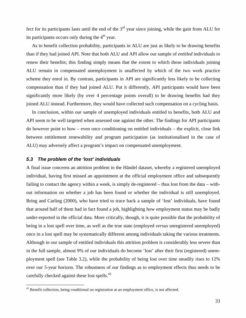
33

fect for its participants lasts until the end of the 3rd year since joining, while the gain from ALU for

its participants occurs only during the 4th year.

As to benefit collection probability, participants in ALU are just as likely to be drawing benefits

than if they had joined API. Note that both ALU and API allow our sample of entitled individuals to

renew their benefits; this finding simply means that the extent to which those individuals joining

ALU remain in compensated unemployment is unaffected by which of the two work practice

scheme they enrol in. By contrast, participants in API are significantly less likely to be collecting

compensation than if they had joined ALU. Put it differently, API participants would have been

significantly more likely (by over 4 percentage points overall) to be drawing benefits had they

joined ALU instead. Furthermore, they would have collected such compensation on a cycling basis.

In conclusion, within our sample of unemployed individuals entitled to benefits, both ALU and

API seem to be well targeted when assessed one against the other. The findings for API participants

do however point to how – even once conditioning on entitled individuals – the explicit, close link

between entitlement renewability and program participation (as institutionalised in the case of

ALU) may adversely affect a program’s impact on compensated unemployment.

5.3 The problem of the ‘lost’ individuals A final issue concerns an attrition problem in the Händel dataset, whereby a registered unemployed

individual, having first missed an appointment at the official employment office and subsequently

failing to contact the agency within a week, is simply de-registered – thus lost from the data – with-

out information on whether a job has been found or whether the individual is still unemployed.

Bring and Carling (2000), who have tried to trace back a sample of ‘lost’ individuals, have found

that around half of them had in fact found a job, highlighting how employment status may be badly

under-reported in the official data. More critically, though, it is quite possible that the probability of

being in a lost spell over time, as well as the true state (employed versus unregistered unemployed)

once in a lost spell may be systematically different among individuals taking the various treatments.

Although in our sample of entitled individuals this attrition problem is considerably less severe than

in the full sample, almost 9% of our individuals do become ‘lost’ after their first (registered) unem-

ployment spell (see Table 3.2), while the probability of being lost over time steadily rises to 12%

over our 5-year horizon. The robustness of our findings as to employment effects thus needs to be

carefully checked against these lost spells.43

43 Benefit collection, being conditional on registration at an employment office, is not affected.

34

Following Sianesi (2004), the additional information from the Bring and Carling survey has been

exploited to perform best- and worst-case bounds analysis on all the pair-wise comparisons of the

treatments.44 These robustness checks, shown in Figures A6 and A7 in the Appendix, leave the con-

clusions discussed above in fact virtually unchanged, in terms of both the differential performance

of the various programs, as well as the positive employment effect of job subsidies and the negative

ones of relief work, ALU and training compared to longer job search.

6. Discussion and conclusions

This paper has investigated the differential performance of six main types of Swedish programs

both relative to one another and vis-à-vis more intense job search in open unemployment.

Starting from the latter comparison, all the programs were found to initially lock in their partici-

pants, significantly reducing their employment probability.45 As to the treatment effects on more

long-term employment prospects as well as on unemployment benefit collection, job subsidies

proved to be an extremely successful measure. Trainee replacement schemes were found to perform

rather satisfactorily, while results for all the other programs have been discouraging.

In particular, individuals joining labour market training, a work practice scheme (API or ALU)

and relief work were found to subsequently display lower employment rates coupled with a higher

benefit collection probability than if they had searched further as openly unemployed.

ALMPs in OECD countries have in fact a mixed track record. Negative effects of public training

programs are far from unheard of; in the US, there is experimental evidence of some of these meas-

ures being ineffective – sometimes even counterproductive – for economically disadvantaged males

and especially youth (see e.g. Heckman et al., 1999, Friedlander et al., 1997). Negative training ef-

fects have also been uncovered in Europe (e.g. recently by Lecher et al., 2005, for Germany, who

link these findings to training participants having become locked in a declining sector).

44 The conditional probability that a lost individual (L=1) with characteristics X has in reality found employment (Y=1) can be decomposed as: P(Y=1|X,L=1) = P(Y=1|X,L=1,D=1)⋅P(D=1|X,L=1) + P(Y=1|X,L=1,D=0)⋅[1–P(D=1|X,L=1)], where for each pair-wise treatment comparison, D=1 denotes the treatment and D=0 the comparison treatment. For each lost individual i, we know treatment his status D, we can estimate his treatment probability given the lost status P(D=1|X,L=1) ≡ D

ip and based on the survey we can impute his misclassification probability P(Y=1|X,L=1) ≡ Yip . In

order to derive worst- and best-case bounds, we assign P(Y=1|X,L=1,D=d) by setting P(Y=1|X,L=1,D=1–d) to its maxi-mum or minimum, compatible with the given D

ip and Yip , as well as with all probabilities being in [0; 1].

45 All survey studies of search activity in Sweden have in fact uncovered sizeable lock-in effects: irrespective of timing, program and age group, individuals on a program search less frequently and in fewer ways than the openly unemployed (see Calmfors et al., 2001, for references).

35

As for Sweden in the mid 90s, several factors may account for the discouraging findings uncov-

ered here. It might be more difficult to put participants back into stable work in periods of high un-

employment, or the massive use of ALMPs in the 90s might have resulted in inefficient program

administration.46, 47 However, an additional most likely explanation relates to the use of programs

simply as a way to re-qualify for unemployment benefits, with programs ending up locking partici-

pants – and in particular those entitled to unemployment compensation – in the unemployment sys-

tem.48 In fact, when exploring the extent to which the treatment effects vary for participants who

joined their program after different amounts of time, we found relief work, API and especially ALU

to be chiefly used as vehicles to escape benefit exhaustion. Note that these are exactly those pro-

grams formally preventing participants from performing labour-market relevant tasks. The first

broad lesson from the Swedish experience thus seems to be that the use of programs predominantly

as ‘parking slots’ for the unemployed and as gateways to renewed entitlement has, maybe unsur-

prisingly, caused job-seekers to drift into long-term unemployment and benefit dependency.

As to the differential effects on employment and compensated unemployment from the pair-wise

comparisons of the programs, job subsidies was again the undisputed best performer, followed by

trainee replacement and – by a very long stretch – labour market training. Relief work and work

practice schemes did not seem to perform in a significantly different way from one another.

Scrutinising the Swedish experience to derive general lessons as to which type of program works

best, we thus found that those programs providing (subsidised) workplace experience and on-the-

job training at an employer are relatively more effective for participants’ subsequent labour market

success than vocational classroom training courses. Furthermore, the more relevant and the closer to

the competitive labour market the kind of task performed, the higher the program ranks.

The similarity of results across studies looking at different countries with varying labour market

structures and policies may in fact indicate a general validity of these overall conclusions. Specifi-

cally, in several OECD countries subsidised employment has been found to have a greater impact

than public training or direct job creation measures (see e.g. the papers in footnote 5 and, for a re-

view, Martin and Grubb, 2001). Recent work comparing the effectiveness of the four options of the

46 Bloom et al. (2001) find evidence that high unemployment as well as large caseloads reduce the impacts of welfare-to-work programs in the US. As to labour market training in Sweden, Calmfors et al. (2001) highlight a switch from positive effects in the 80s to negative ones in the 90s. 47 By contrast, stigma effects from program participation are not likely to apply in Sweden, where employers view for-mer participants more favourably than openly unemployed individuals (see the survey studies in Calmfors et al., 2001).

36

New Deal for Young People in the UK similarly finds that the employment option performs best

compared to full-time education and training, the voluntary sector and the environmental task force

(Bonjour et al., 2001; Dorsett, 2004). The finding that the ‘work first’ approach of the employment

program dominates the human capital approach of the training measure is also in line with the meta-

analysis of US welfare-to-work programs by Greenberg et al. (2004).49

Turning to the cost side, it is quite remarkable to notice how the ranking of the programs in

terms of their effectiveness is roughly reversed when taken in terms of their expensiveness.

It is however important not to jump to the hasty conclusion that job subsidies are the solution –

the most effective program as well as the cheapest. Several issues can be raised both in terms of the

effective magnitude of the uncovered effects and in terms of their general applicability should the

scope of the program be extended. A first issue concerns the validity of the CIA assumption for par-

ticipants in this program: since job subsidies informally entail the expectation that the engagement

will then continue, it is likely that potential candidates are considered quite carefully. Even though

we control for a host of factors underlying the caseworker’s judgement, it may still be the case that

subsidised participants are slightly ‘better’ on average than matched comparisons. Still, it would be

hard to argue that remaining selection bias could account for all of the very large positive effects

seemingly displayed by job subsidies in terms of all comparisons and outcomes considered.

Even if the direction of the estimated effects may appear reliable, though, it may not be possible

or even desirable to focus attention and funds on this kind of measure. As to the sheer possibility of

extending it, scope is in fact limited: the public sector cannot use such grants, and following EU

regulations in 1997 neither do employers in the synthetic fibre, automotive, steel, shipyard, fishery

and transport industries. Apart from legal feasibility, the desirability of a widespread use of this

measure may not be warranted once it is considered that our estimates ignore potential indirect and

48 Findings in Sianesi (2001 and 2004) considering the overall program system lend support to the conjecture that for individuals entitled to unemployment compensation, the eligibility renewability rules can significantly distort the incen-tives for participation and wipe out potential productivity-enhancing effects of the programs. 49 The US literature is not directly comparable to the present, and more generally, to European evaluations. Apart from mainly looking at a different outcome (earnings rather than employment) and target population (the economically dis-advantaged rather than displaced workers), the US literature on ‘employment subsidy measures’ has in fact looked at treatments which include not only hiring subsidies, but also public service employment (the counterpart of relief work in Sweden) and temporary work experience in the public and non-profit sectors (the counterpart of work practice). The definition of treatment (see Heckman et al., 1999, table 1) is thus largely different too, and in fact likely to account for why these ‘employment subsidy measures’ have at times been found to be ineffective, especially for males, in the US. An additional problem, mentioned in the introduction, is that the US programs mostly come as packages of different measures, which makes it very hard to isolate where the effect is coming from. For example, Friedlander et al. (1997) point out that it remains unclear whether the positive earnings effects from JTPS stem from skills acquisition, program assistance, or the wage subsidy given to employers as part of the activity.

37

general equilibrium effects which may spill over to other groups. In particular, substitution would

take place if participants in the job subsidy program were to take (some of) the jobs that participants

in the other programs or ‘waiting’ unemployed individuals would have been offered in the absence

of the subsidies. The impact of the subsidy would thus be at the expense of worsened conditions

either for participants in other programs or for openly unemployed individuals finding it more diffi-

cult to get jobs. The estimated effect would in this case overestimate the net social impact of the

subsidy program. Both survey and econometric Swedish studies do in fact find sizeable (around 65-

70%) direct displacement effects arising from those Swedish programs that generate subsidised em-

ployment.50 Finally, it is obviously unthinkable to generalise such a measure to all unemployed job-

seekers: it would simply become just a way to subsidise firms’ hirings, resulting in huge dead-

weight effects (i.e. subsidising hiring that would have taken place anyway).

In the light of our results and of the above considerations, a more promising measure might ap-

pear to be trainee replacement. Still among the cheapest, it was shown to perform quite satisfacto-

rily. In fact, it shares some of the features likely to be at the root of the success of job subsidies:

during the temporary employment spell it provides relevant job-specific training and can be used as

a cheap screening device of individual unobserved productivity. At the same time it sends out a

message that the individual has been gaining (or maintaining) relevant skills, thus making the job-

seeker more attractive to potential future employers, who value the fact that a job is being per-

formed in the regular competitive market.51 Finally, our partial-equilibrium estimates are likely to

underestimate the program’s full effect, since they do not take into account the ‘double-dividend’

arising from the possibility offered to the replaced employees of increasing their human capital

through training. Nevertheless, a few issues call once again for caution. The ‘double-dividend’ from

the subsidised training of the replaced employee may in fact often turn out to be dead-weight loss

instead52, while Harkman et al. (1999) found evidence of dead-weight in terms of the deputies as

well, with a large share of participants alternating between regular short-term jobs and trainee re-

50 These results come from the Swedish macro studies (reviewed in Calmfors et al., 2001), but apply more generally. Using macro data for OECD countries, Boone and Van Ours (2004) find that expenditure on labour market training is most effective, on public employment services has some effect and on subsidized jobs is not effective at all in bringing down aggregate unemployment. 51 These arguments are in line with the complaint by Swedish employers about the excessively large number of labour market measures, which prevents them from being able to make informed judgements as to the exact content and value of each program. Part of the success of job subsidies and trainee replacement may thus stem from the fact that they offer firms a cheap way to screen workers’ productivity in regular and known activities. 52 Since 80 to 90% of employers taking part in the scheme are within sectors (health care and related branches in the public sector) with a long-standing system for further training funded by the employer, it seems likely that a good part of the sponsored training would have occurred anyway. (I thank Anders Harkman for this information.)

38

placement with the same employer. Finally, survey studies have in fact uncovered displacement ef-

fects of the same order as job subsidies (e.g. AMS, 1998).53

In conclusion, this analysis unambiguously joins previous micro studies in finding that the more

it resembles regular employment in the competitive labour market, the higher the program’s bene-

fits to its participants. It is however essential to consider this evidence in the light of that arising

from the macroeconomic literature, which has widely documented that exactly for these types of

programs the potential for negative crowding-out and dead-weight effects is largest.54 Taken to-

gether, the various results clearly highlight a difficult trade off to be faced by labour market policy.

References Ackum Agell, S. (1995), Swedish labour market programs: Efficiency and timing, Swedish Eco-

nomic Policy Review, 2, 65-98. AMS (1998), Undanträngningseffekter av arbetsmarknadspolitiska åtgärder – enenkätundersökning

ur både arbetssökande- och arbetsgivarperspektiv, Ura 1998:8, AMS. Bonjour, D., Dorsett, R., Knight, G., Lissenburgh, S., Mukherjee, A., Payne, J., Range, M., Urwin,

P., & White, M. (2001), “New Deal for Young People: National Survey of Participants: Stage 2”, Employment Service Research and Development Report ESR67, Employment Service, Sheffield, UK.

Bonnal, L., Fougère, D. and Sérandon, A. (1997), Evaluating the impact of French employment policies on individual labour market histories, Review of Economic Studies, 67, 683-713.

Bring, J., and Carling, K., (2000), Attrition and misclassification of drop-outs in the analysis of un-employment duration, Journal of Official Statistics, 4, 321-330.

Bloom, H.S, Hill, C.J. and Riccio, J. (2001), “Modeling the performance of welfare-to-work pro-grams: The effects of program management and services, economic environment, and client characteristics”, MDRC Working Papers on Research Methodology, New York, June.

Boone, J. and Van Ours, J.C. (2004), “Effective Active Labour Market Policies”, CEPR Discussion Paper 4707, London.

Brodaty, T., Crépon, B. and Fougère, D. (2001), Using matching estimators to evaluate alternative youth employment programs: Evidence from France, 1986-8, in Lechner, M., Pfeiffer, F. (eds), Econometric Evaluation of Labour Market Policies, Physica/Springer, Heidelberg.

Calmfors, L. Forslund A. and Hemström, M. (2001), Does active labour market policy work? Les-sons from the Swedish experiences, Swedish Economic Policy Review, 8, 61-124.

Carling, K. and Larsson, L. (2000a), Utvärdering av arbetsmarknadsprogram i Sverige: Rätt svar är viktigt, men vilken var nu frågan?, Arbetsmarknad&Arbetsliv, 6, 185-192.

Carling, K. and Larsson, L. (2000b), Replik till Lars Behrenz och Anders Harkman, Ar-betsmarknad&Arbetsliv, 6, 278-281.

Carling, K. and Richardson, K. (2004), The relative efficiency of labour market programs: Swedish experience from the 1990s, Labour Economics, 11, 335-354.

53 As an average across survey studies, 42 percent (see Calmfors et al., 2001). 54 See in particular the evidence reviewed in Calmfors et al. (2001).

39

Dorsett, R. (forthcoming) “The New Deal for Young People: Effect on the labour market status of young men”, Labour Economics,

European Commission (1998), From guidelines to actions: The National Action Plans for Employ-ment, Directorate-General for Employment, Industrial Relations and Social Affairs, Luxemburg.

Fredriksson, P. and Johansson, P. (2003), Program evaluation and random program starts, Uppsala University Working Paper 2003:1.

Friedlander, D., Greenberg, D.H and Robins, P.K. (1997), Evaluating government training programs for the economically disadvantaged, Journal of Economic Literature, 4, 1809-55.

Frölich, M. (2001), Treatment choice based on semiparametric evaluation methods, Discussion Pa-per 2001-16, Department of Economics, University of St. Gallen.

Frölich, M., Heshmati, A., and Lechner, M. (2004), A microeconometric evaluation of rehabilita-tion of long-term sickness in Sweden, Journal of Applied Econometrics, 19, 375-396.

Garfinkel, I., Manski, C.F and Michalopoulos, C. (1992), Micro experiments and macro effects, in Manski, C.F. and Garfinkel, I. (eds), Evaluating Welfare and Training Programs, Cambridge: Harvard University Press, 253-273.

Gerfin, M. and Lechner, M. (2002), Microeconometric evaluation of the active labour market policy in Switzerland, Economic Journal, 112, 854-893.

Gerfin, M., Lechner, M. and Steiger, H. (2004), Does subsidised temporary employment get the un-employed back to work? An econometric analysis of two different schemes, forthcoming La-bour Economics.

Greenberg, D., Ashworth, K., Cebulla, A. and Walker, R. (2004), “Do welfare-to-work programmes work for long?”, Fiscal Studies, 25, 1, 27-53.

Ham, J.C. and LaLonde, R.J. (1996), “The Effect of Sample Selection and Initial Conditions in Du-ration Models: Evidence from Experimental Data on Training”, Econometrica, 64, 175-205.

Hallström, N.E. (1994), Genomförandet av åtgärden arbetslivsutveckling. En studie i sex kommu-ner i tre län, Mimeo, Department of Culture and Social Sciences, Linköping University.

Harkman, A. (2000), Vem placeras i åtgärd?, Mimeo, Office of Labour Market Policy Evaluation, Uppsala.

Harkman, A., Johansson, A. and Okeke, S. (1999), Åtgärdsundersökning 1998, Ura 1999:1, AMS. Heckman, J.J., Ichimura, H., Smith, J.A. and Todd, P.E. (1998), Characterising selection bias using

experimental data, Econometrica, 66, 1017-1098. Heckman, J.J., LaLonde, R.J. and Smith, J.A. (1999), The economics and econometrics of active

labour market programs, in Ashenfelter, O. and Card, D. (eds.), The Handbook of Labour Eco-nomics, 3, Ch.31, North-Holland, Amsterdam.

Imbens, G. (2000), The role of propensity score in estimating dose-response functions, Biometrika, 87, 706-710.

Larsson, L. (2003), Evaluation of Swedish youth labour market programmes, Journal of Human Resources, 38, 891-927.

Layard, R., Nickell, S. and Jackman, R. (1991), Unemployment, Macroeconomic Performance and the Labour Market, Oxford University Press.

Lechner, M. (2001), Identification and estimation of causal effects of multiple treatments under the conditional independence assumption, in Lechner, M., Pfeiffer, F. (eds), Econometric Evalua-tion of Labour Market Policies, Physica/Springer, Heidelberg, 43-58.

Lechner, M., Miquel, R. and Wunsch, C. (2005), “The Curse and Blessing of Training the Unem-ployed in a Changing Economy: The Case of East Germany after Unification”, Discussion Pa-per, Department of Economics, University of St.Gallen.

40

Lechner, M. and Smith, J.A. (2003), What is the value added by caseworkers?, IZA Discussion Pa-per 728.

Lundin, M. and Skedinger, P. (2000), Decentralisation of active labour market policy: The case of Swedish Local Employment Service Committees, IFAU Working Paper 2000:6, Office of La-bour Market Policy Evaluation, Uppsala.

Martin, J.P. and Grubb, D. (2001), What works and for whom: A review of OECD countries’ ex-periences with active labour market policies, Swedish Economic Policy Review, 8, 9-56.

Moffitt, R. (1992), Evaluation methods for program entry effects, in Manski, C.F. and Garfinkel, I. (eds), Evaluating Welfare and Training Programs, Cambridge: Harvard University Press, 231-52.

OECD (1996), The OECD Jobs Strategy: Enhancing the Effectiveness of Active Labour Market Policies, Paris: OECD Publications.

OECD (1994), The OECD Jobs Study: Evidence and Explanations, Paris: OECD Publications. Ridder, G. (1986), An event history approach to the evaluation of training, recruitment and em-

ployment programs, Journal of Applied Econometrics, 1, 109-126. Rosenbaum, P.R. and Rubin, D.B. (1983), The central role of the propensity score in observational

studies for causal effects, Biometrika, 70, 41-55. Rosenbaum, P.R. and Rubin, D.B. (1985), Constructing a control group using multivariate matched

sampling methods that incorporate the propensity score, The American Statistician, 39, 33-38. Rubin, D.B. (1980), Discussion of ‘Randomisation analysis of experimental data in the Fisher ran-

domisation test’ by Basu, Journal of the American Statistical Association, 75, 591-593. Sianesi, B. (2001), Swedish active labour market programs in the 1990s: Overall effectiveness and

differential performance, Swedish Economic Policy Review, 8, 133-169. Sianesi, B. (2004), An evaluation of the Swedish system of active labour market programs in the

1990s, Review of Economics and Statistics, 1, 133-155. Swedish Institute (1997), Swedish Active Labour Market Policy, Fact Sheets on Sweden, Stock-

holm, June.

Appendix A. Technical Appendix In this Appendix the framework of Imbens (2000) and Lechner (2001), which generalises

Rosenbaum and Rubin’s (1983) binary potential outcome approach to the multiple-treatment case,

is adapted to the institutional set-up and evaluation questions described in Section 4.1.

Let U, elapsed unemployment duration since inflow into unemployment, be viewed as discrete

and measured in months. The population of interest (eligibles) at time u are those still openly un-

employed after u months. The eligibles at u can choose from a set of K+1 mutually exclusive

‘treatments’: joining one of the K=6 programs or waiting longer than u in open unemployment. In-

terest lies in the causal average effect of a treatment relative to another treatment on individual la-

bour market status over time, ( ){ }u Tt t uY = (in our application T=60 months). The (u) superscript is a

reminder that the time series of outcomes ( )utY starts being defined from t=u, u+1, …, T and possi-

bly depends on treatment exposure at u. A set of potential outcomes at t (t≥u) is correspondingly

associated to each of the K+1 treatments: 0( )utY , 1( )u

tY , …, ( )K utY with ( )k u

tY (k≠0) denoting the poten-

tial outcome at t if joining program k in one’s uth month and 0( )utY the potential outcome at t if not

joining any program at least up until u.

Let D(u)∈{0, 1, …, K} denote actual treatment assignment, that is D(u)=k if joining program k at u

and D(u)=0 if not joining any (at least up to) u.1 Since any given individual receives only one of the

treatments, his remaining K potential outcomes are unobserved counterfactuals.

We are interested in the generalisation of the ‘effect of treatment on the treated’: the (K+1)K

pair-wise comparisons of the average effect of treatment k relative to treatment k' conditional on

assignment to treatment k. Specifically, for each u, interest lies in the time series of ( , ')ut k k∆ , the

average impact at time t, for those joining program k in their uth month of unemployment, of joining

program k at u compared to receiving a different treatment k' at u:

( , ')ut k k∆ ≡ E( ( )k u

tY – '( )k utY | D(u)=k) = E( ( )k u

tY | D(u)=k) – E( '( )k utY | D(u)=k) (1)

1 For this representation to be meaningful, the stable-unit-treatment-value assumption (SUTVA –

Rubin, 1980) has to be fulfilled, requiring treatment status as well as all the potential outcomes of a

given individual to be independent from the treatment status of others, the latter ruling out the pos-

sibility of general equilibrium effects.

for t=u, u+1, …T and for k∈{1, …, K}, k'∈{0, 1, …, K}, k≠k’.

Since the observed program duration is endogenous, measurement of ( , ')ut k k∆ starts at time u;

the program treatments have in fact been defined as joining a given program (in a given month), so

that the causal effect starts to work upon joining. Note in particular that the comparison group for

( ,0)ut k∆ is made up of all those still unemployed at u, irrespective of what happens after u. Some

of them may later go on a program, while some others may find a job before ever joining one. For

both comparisons and those joining a program at u, whatever happens after u is viewed as an out-

come of the joining versus waiting decision at u. Finally note that the various treatment effects by

month u are always based on a comparison of individuals who have reached the same elapsed dura-

tion in unemployment: some join program A at u, some join program B at u and some do not join

any program at least up to u.2

To identify all the counterfactuals E( '( )k utY | D(u)=k), we invoke an extension of the conditional in-

dependence assumption that conditional on the value of observables X, the (counterfactual) distribu-

tion of '( )k utY for individuals joining program k after u months is the same as the (observed) distribu-

tion of '( )k utY for individuals joining program k' at u or, for k'=0, deciding to wait longer than u:3

D(u) ⊥ ( ( )k utY , '( )k u

tY ) | X=x, D(u)∈{k, k'} for k, k'∈{0, 1, …, K}, k≠k' and t=u, u+1, …T (2)

The unobserved counterfactuals can thus be identified:

E( '( )k utY | D(u)=k) = EX [E( '( )k u

tY | D(u)=k, X) | D(u)=k] = EX[E( '( )k utY | D(u)=k', X) | D(u)=k]

with the inner expectation identified due to (2) and the outer expectation taken with respect to the

distribution of X for participants in k. The latter highlights how in order to adjust for differences in

X, all participants in k need to have a counterpart in the k'-group. Let the (generalised) propensity

score pk(X; u) be the conditional probability of receiving treatment k after u months in unemploy-

ment: pk(X; u) ≡ Pr(D(u)=k | X=x). The common support requirement for all pair-wise conditional

parameters then translates into: 0<pk(X; u)<1 for k=0, 1, …, K. 4

2 Those joining a program or finding a job drop out of the eligibles exposed to the treatments in

later months. 3 Its weaker form in terms of conditional mean independence would suffice. 4 To just compare treatment k with k' for participants in k, one would need to have some participants

in k' with those X’s at which there are participants in k, i.e. pk'(X; u)>0 ∀X: pk(X: u)>0.

The treatment effects by month of entry, ( , ')ut k k∆ , can then be averaged over the observed entry

distribution in program k:

max max( ) ( ) '( ) ( )1 1

( , ') [ ( , ') | ]

( | ) ( | ) ( ) ( , ')

ut U t

U Uu k u k u u u ut t tu u

k k E k k D k

Pr D k D k E Y Y D k k k kω= =

∆ ≡ ∆ =

= = = − = ≡ ⋅∆∑ ∑ (3)

with D=k denoting participants in program k at any time and Umax the longest observed pre-program

unemployment duration, so that Pr(D=k)= max1u

U=∑ Pr(D(u)=k). The weights ω u(k) ≡ Pr(D(u)=k | D=k)

are given by the share of participants in program k observed to join that program at the various

months u.

For the various program-to-program comparisons – i.e. for k'∈{1, …, 6} – the parameters in (3)

have the usual causal interpretation as the average effect of joining program k compared to joining

program k' for those observed to enter program k, and are thus directly informative of the relative

performance of the different programs. Stratifying by month of entry is simply a careful way to con-

trol for (or match on) unemployment duration before joining the respective program.

As to the separate effectiveness of the single programs compared to longer search in open unem-

ployment – i.e. for k'=0 – however, the parameters in (3) no longer have a straightforward causal

interpretation given to the indeterminate nature of Y0. Though for this comparison it is the effects by

month of entry ( ,0)ut k∆ that have a clear causal interpretation, their algebraic weighted average in

(3) allows one to gain a synthetic overview of their general patterns and can be useful as a more

concise summary measure.

B. Selected descriptive statistics, by type of exit from first open unemployment spell Program participants Exits from unemployment Training ALU API Relief Replac. Subsidy Employed Inactivity Education Attrition

Female 43.5 43.7 50.4 26.8 79.3 33.8 47.0 77.4 66.2 49.5 Age (years) 38.4 40.5 36.5 39.6 37.6 38.5 37.7 34.5 32.8 37.1 Foreign citizen 6.1 7.4 21.2 9.2 3.7 4.7 4.6 7.1 5.9 10.2 Educ.: Compulsory 29.6 33.5 35.3 33.6 18.0 32.6 26.0 24.8 22.2 30.4 Secondary 8.7 7.9 7.3 7.2 6.4 7.0 6.5 10.4 16.8 9.2 Sec. vocational 53.2 41.0 35.3 50.2 48.9 47.4 45.2 45.0 41.2 39.5 University 8.5 17.6 22.1 9.0 26.7 12.9 22.3 19.8 19.8 20.9 Has education for job 64.5 64.6 59.1 66.9 77.4 67.6 73.5 67.9 54.6 64.4 Experience: None 6.1 7.5 19.3 5.5 11.0 3.5 5.3 7.1 15.2 6.8 Some 9.8 12.0 15.5 11.8 17.0 12.7 11.5 15.2 19.6 14.2 Much 83.5 79.9 64.2 82.7 71.6 83.1 82.7 76.1 59.3 77.9 KAS 5.9 6.2 13.6 14.7 5.2 12.7 8.2 6.1 6.2 15.8 Daily wage (SEK) 641.1 667.7 601.9 665.1 555.2 646.6 665.3 590.8 587.4 617.0 Worked 20h/week 1.1 2.4 2.4 2.8 2.1 2.3 1.4 2.2 2.0 2.1 Worked 30h/week 3.2 2.8 3.5 1.7 7.2 1.2 4.1 4.7 5.5 4.4 Worked 40h/week 84.4 83.1 79.8 86.2 67.7 87.6 81.1 75.2 72.6 76.6 Sector: Professional, technical 8.7 15.2 15.3 9.2 16.6 12.7 14.8 11.6 16.0 13.7 Health, nursing, social 6.6 9.9 7.3 5.7 51.3 3.5 16.0 24.0 23.3 17.0 Admin, managerial, 19.7 16.5 18.1 6.4 8.7 16.4 13.4 17.6 16.1 12.0 Sales 12.1 13.4 15.1 9.0 5.2 23.0 10.5 13.6 10.6 12.7 Agric., forest, fishery 0.9 1.8 0.7 3.2 0.2 1.9 2.2 1.3 1.2 1.4 Transport, communica- 6.4 5.0 4.9 4.8 2.3 8.5 5.8 4.6 3.8 6.8 Production 31.5 25.2 18.6 48.8 6.0 22.5 26.2 11.0 11.0 18.9 Services 10.2 10.1 14.6 10.0 9.1 8.9 9.7 13.6 9.6 15.1 Other 3.8 2.9 5.4 2.9 0.6 2.6 1.4 2.7 8.4 2.5 Looks for part-time job 3.9 6.5 5.6 4.0 9.7 4.2 7.2 11.8 6.7 7.8 Interlocal job seeking 17.7 15.3 15.5 17.3 12.2 13.4 14.6 8.5 8.4 11.6 Part-time unemployed 11.4 12.2 22.1 7.4 35.2 15.3 33.0 36.6 21.3 38.2 Caseworker judgementa: Job ready 91.5 95.5 92.9 95.9 91.5 97.4 81.6 76.6 83.6 77.2 Needs guidance 16.2 11.3 19.1 10.6 4.6 7.7 3.2 6.5 6.4 5.9 Offered a program 9.7 3.9 8.0 4.3 0.6 3.5 0.5 0.7 0.5 0.9 Difficult to place 5.9 2.5 4.0 1.5 1.2 2.1 2.0 11.4 7.2 5.4 Local program rate 24.9 24.5 25.3 24.1 24.2 23.7 23.3 23.5 18.8 23.3 County: Stockholm 6.0 19.6 32.0 26.1 9.9 30.5 22.2 20.2 25.9 35.8 Malmöhus 21.2 13.4 10.8 9.4 13.9 14.8 12.6 12.9 12.7 13.6 Göteborg/M. 11.6 18.3 22.1 16.1 12.2 13.8 15.1 16.7 16.9 14.3 Month of entry: Jan 15.8 13.9 6.1 19.8 16.4 8.7 16.6 15.3 7.2 13.7 Jun 11.0 9.6 8.7 6.6 10.1 10.6 10.1 9.9 33.3 10 Dec 5.1 6.0 13.4 5.5 5.0 10.3 6.5 6.0 3.9 6.1 Median unempl. duration 182 365 456 213 152 304 122 213 91 274 Median progr. duration 91 154 154 147 105 153 Number 1,387 2,983 425 654 483 426 15,972 2,680 2,456 2,739

Note: Age is measured at entry into unemployment; all other time-varying variables at program entry or at de-registration. a Caseworkers’ assessment can be updated during the unemployment spell; the figures thus add up to over 100.

C. Indicators of matching quality Treatment N1

Comparison N0 Probit ps-R2

before (1) Probit ps-R2

after (2) Pr>χ2 after (3)

Med bias before (4)

Med biasafter (5)

% lost to CS (6)

training 1384 waiting 0.0155 0.7474 2.19 0.0 ALU 2973 waiting 0.0096 0.1452 1.92 0.2 API 425 waiting 0.0403 0.9592 3.60 0.2 relief 652 waiting 0.0244 0.9829 2.69 0.0 replacement 483 waiting 0.0216 0.9679 3.34 0.0 subsidy 426 waiting 0.0296 0.9994 3.05 0.0 training 1384 work practice 3398 0.2417 0.0095 0.5772 6.15 1.48 0.0 relief 652 0.2558 0.0344 0.0110 10.01 3.72 4.4 replacement 483 0.4054 0.0407 0.0073 10.61 4.20 10.4 subsidy 426 0.2888 0.0982 0.0000 10.11 4.93 1.7 work practice 3398 training 1384 0.2417 0.0296 0.0000 6.15 2.90 1.3 relief 652 0.1547 0.0464 0.0000 8.34 4.49 1.8 replacement 483 0.3606 0.1280 0.0000 10.16 6.09 0.0 subsidy 426 0.1398 0.0225 0.0011 6.42 2.30 2.1 relief 652 training 1384 0.2558 0.0165 0.9577 10.01 2.23 1.5 work practice 3398 0.1547 0.0047 1.0000 8.12 1.70 0.0 replacement 483 0.5336 0.3079 0.0000 15.45 6.87 0.0 subsidy 426 0.2677 0.0132 0.0000 9.50 5.89 0.0 replacement 483 training 1384 0.4054 0.0429 0.0011 10.45 4.24 9.73 work practice 3398 0.3606 0.0192 0.0034 10.12 2.42 4.34 relief 652 0.5336 0.4997 0.0000 15.12 8.93 0.0 subsidy 426 0.5609 0.4800 0.0000 12.82 6.43 0.0 subsidy 426 training 1384 0.2888 0.0218 0.8349 10.12 2.86 0.5 work practice 3398 0.1398 0.0045 1.0000 6.43 1.32 1.6 relief 652 0.2677 0.0453 0. 3931 9.50 3.38 0.0 replacement 483 0.5609 0.4844 0.0000 12.81 4.68 0.0 ALU 2973 API 425 0.2523 0.0508 0.0000 11.12 4.00 27.9 API 425 ALU 2973 0.2523 0.0071 0.9995 11.18 1.29 1.4

Notes:

Work practice is API and ALU combined. (1) Pseudo-R2 from a Probit of D on X, giving an indication of how well the regressors X explain the participation probability. (2) Pseudo-R2 from a Probit of D on X on the matched samples, to be compared to (1). (3) P-value of the likelihood-ratio test after matching, testing the null of joint insignificance of all the regressors. (Before match-

ing, Pr>χ2=0.0000 always). (4), (5) Median absolute standardised bias before and after matching, median taken over all the regressors.

Following Rosenbaum and Rubin (1985), for a given covariate X, the standardised difference before matching is the differ-ence of the sample means in the full treated and non-treated sub-samples as a percentage of the square root of the average of the sample variances in the full treated and non-treated groups. The standardised difference after matching is the difference of the sample means in the matched treated (i.e. falling within the common support) and matched non-treated sub-samples as a percentage of the square root of the average of the sample variances in the full treated and non-treated groups.

( )1 0

1 0

( ) 100( ) ( ) / 2

beforeX X

B XV X V X

−≡ ⋅

+

( )1 0

1 0

( ) 100( ) ( ) / 2

M Mafter

X XB X

V X V X−

≡ ⋅+

The standardization allows comparisons between variables and, for a given variable, comparisons before and after matching. (6) Percentage of the treated individuals falling outside of the common support.

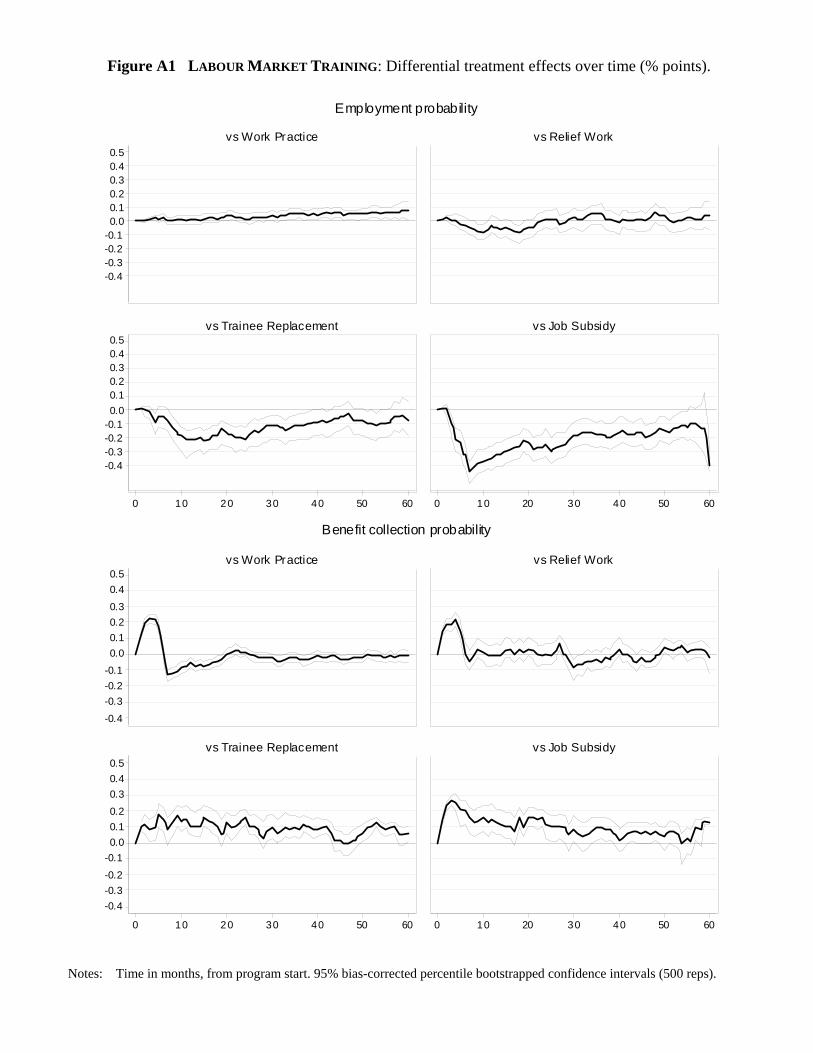
Figure A1 LABOUR MARKET TRAINING: Differential treatment effects over time (% points).

-0.4-0.3-0.2-0.10.00.10.20.30.40.5

-0.4-0.3-0.2-0.10.00.10.20.30.40.5

0 10 20 30 40 50 60 0 10 20 30 40 50 60

vs Work Practice vs Relief Work

vs Trainee Replacement vs Job Subsidy

Employment probability

-0.4

-0.3-0.2-0.10.00.10.20.3

0.40.5

-0.4-0.3-0.2

-0.10.00.10.20.30.40.5

0 10 20 30 40 50 60 0 10 20 30 40 50 60

vs Work Practice vs Relief Work

vs Trainee Replacement vs Job Subsidy

Benefit collection probability

Notes: Time in months, from program start. 95% bias-corrected percentile bootstrapped confidence intervals (500 reps).

Figure A2 WORK PRACTICE : Differential treatment effects over time (% points).

-0.4-0.3-0.2-0.10.00.10.20.30.40.5

-0.4-0.3-0.2-0.10.00.10.20.30.40.5

0 10 20 30 40 50 60 0 10 20 30 40 50 60

vs Labour Market Training vs Relief Work

vs Trainee Replacement vs Job Subsidy

Employment probability

-0.4

-0.3-0.2-0.10.00.10.20.3

0.40.5

-0.4-0.3-0.2

-0.10.00.10.20.30.40.5

0 10 20 30 40 50 60 0 10 20 30 40 50 60

vs Labour Market Training vs Relief Work

vs Trainee Replacement vs Job Subsidy

Benefit collection probability

Notes: Time in months, from program start. 95% bias-corrected percentile bootstrapped confidence intervals (500 reps).

Figure A3 RELIEF WORK: Differential treatment effects over time (% points).

-0.4-0.3-0.2-0.10.00.10.20.30.40.5

-0.4-0.3-0.2-0.10.00.10.20.30.40.5

0 10 20 30 40 50 60 0 10 20 30 40 50 60

vs Labour Market Training vs Work Practice

vs Trainee Replacement vs Job Subsidy

Employment probability

-0.4

-0.3-0.2-0.10.00.10.20.3

0.40.5

-0.4-0.3-0.2

-0.10.00.10.20.30.40.5

0 10 20 30 40 50 60 0 10 20 30 40 50 60

vs Labour Market Training vs Work Practice

vs Trainee Replacement vs Job Subsidy

Benefit collection probability

Notes: Time in months, from program start. 95% bias-corrected percentile bootstrapped confidence intervals (500 reps).

Figure A4 TRAINEE REPLACEMENT: Differential treatment effects over time (% points).

-0.4-0.3-0.2-0.10.00.10.20.30.40.5

-0.4-0.3-0.2-0.10.00.10.20.30.40.5

0 10 20 30 40 50 60 0 10 20 30 40 50 60

vs Labour Market Training vs Work Practice

vs Relief Work vs Job Subsidy

Employment probability

-0.4

-0.3-0.2-0.10.00.10.20.3

0.40.5

-0.4-0.3-0.2

-0.10.00.10.20.30.40.5

0 10 20 30 40 50 60 0 10 20 30 40 50 60

vs Labour Market Training vs Work Practice

vs Relief Work vs Job Subsidy

Benefit collection probability

Notes: Time in months, from program start. 95% bias-corrected percentile bootstrapped confidence intervals (500 reps).

Figure A5 JOB SUBSIDIES: Differential treatment effects over time (% points).

-0.4-0.3-0.2-0.10.00.10.2

0.30.40.5

-0.4-0.3-0.2-0.10.00.10.20.30.40.5

0 10 20 30 40 50 60 0 10 20 30 40 50 60

vs Labour Market Training vs Work Practice

vs Relief Work vs Trainee Replacement

Employment probability

-0.4

-0.3-0.2-0.10.00.10.20.3

0.40.5

-0.4-0.3-0.2

-0.10.00.10.20.30.40.5

0 10 20 30 40 50 60 0 10 20 30 40 50 60

vs Labour Market Training vs Work Practice

vs Relief Work vs Trainee Replacement

Benefit collection probability

Notes: Time in months, from program start. 95% bias-corrected percentile bootstrapped confidence intervals (500 reps).

Figure A6 Treatment effects on employment probability over time of joining a given program compared to waiting longer in open unemployment: Estimated effects and best- and worst- case bounds

-0.4-0.3-0.2-0.10.00.10.20.30.40.5

-0.4-0.3-0.2-0.10.00.10.20.30.40.5

-0.4-0.3-0.2-0.10.00.10.20.30.40.5

0 10 20 30 40 50 60 0 10 20 30 40 50 60

Labour Market Training Work Practice - ALU

Work Practice - API Relief Work

Trainee Replacement Job Subsidy

Figure A7 Differential treatment effects on employment probability over time: Estimated effects and best- and worst- case bounds

Labour Market Training

-0 .4

-0 .3

-0 .2

-0 .1

0 .0

0 .1

0 .2

0 .3

0 .4

0 .5

-0 .4

-0 .3

-0 .2

-0 .1

0 .0

0 .1

0 .2

0 .3

0 .4

0 .5

0 10 20 30 40 50 60 0 10 20 30 40 50 6 0

vs Wo rk Pra ctice vs Re lief W ork

vs Traine e R ep la cem ent vs Job Subsidy

Work Practice

-0.4

-0.3

-0.2

-0.1

0.0

0.1

0.2

0.3

0.4

0.5

-0.4

-0.3

-0.2

-0.1

0.0

0.1

0.2

0.3

0.4

0.5

0 10 20 30 40 50 60 0 10 20 30 40 50 6 0

vs Lab our M arket Training vs Re lief W ork

vs Traine e Rep la cem ent vs Job Subsidy

Relief Work

-0.4

-0.3

-0.2

-0.1

0.0

0.1

0.2

0.3

0.4

0.5

-0.4

-0.3

-0.2

-0.1

0.0

0.1

0.2

0.3

0.4

0.5

0 10 20 30 40 50 60 0 10 20 30 40 50 6 0

vs Lab our M arket Training vs W ork Practice

vs Traine e Rep la cem ent vs Job Subsidy

Trainee Replacement

-0.4

-0.3

-0.2

-0.1

0.0

0.1

0.2

0.3

0.4

0.5

-0.4

-0.3

-0.2

-0.1

0.0

0.1

0.2

0.3

0.4

0.5

0 10 20 30 40 50 60 0 10 20 30 40 50 6 0

vs Labour Market Training vs Work Practice

vs Relief Work vs Job Subsidy

Job Subsidies

-0 .4

-0 .3

-0 .2

-0 .1

0 .0

0 .1

0 .2

0 .3

0 .4

0 .5

-0 .4

-0 .3

-0 .2

-0 .1

0 .0

0 .1

0 .2

0 .3

0 .4

0 .5

0 10 20 30 40 50 60 0 10 20 30 40 50 6 0

vs Lab our M arket T raining vs W ork Practice

vs Re lief Wo rk vs Train ee R ep la cem ent